Modelling and measuring maps of nerve connections

PART B

David WillshawInstitute for Adaptive & Neural Computation

School of InformaticsUniversity of Edinburgh

willshaw@inf.ed.ac.uk

2

I now need to apply my method to contemporary data

Instrinsic imaging

3

4

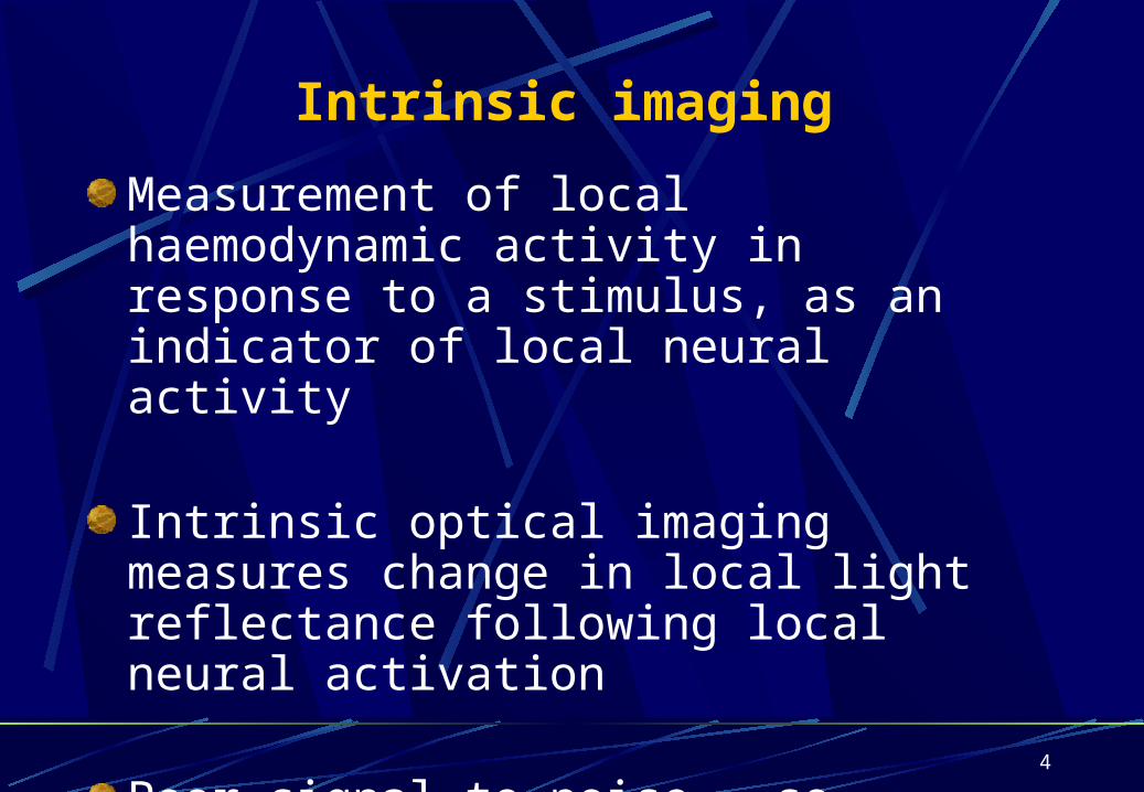
Intrinsic imaging

Measurement of local haemodynamic activity in response to a stimulus, as an indicator of local neural activity

Intrinsic optical imaging measures change in local light reflectance following local neural activation

Poor signal to noise – so averaging is done over many episodes of presentation

Response characteristics

5

6

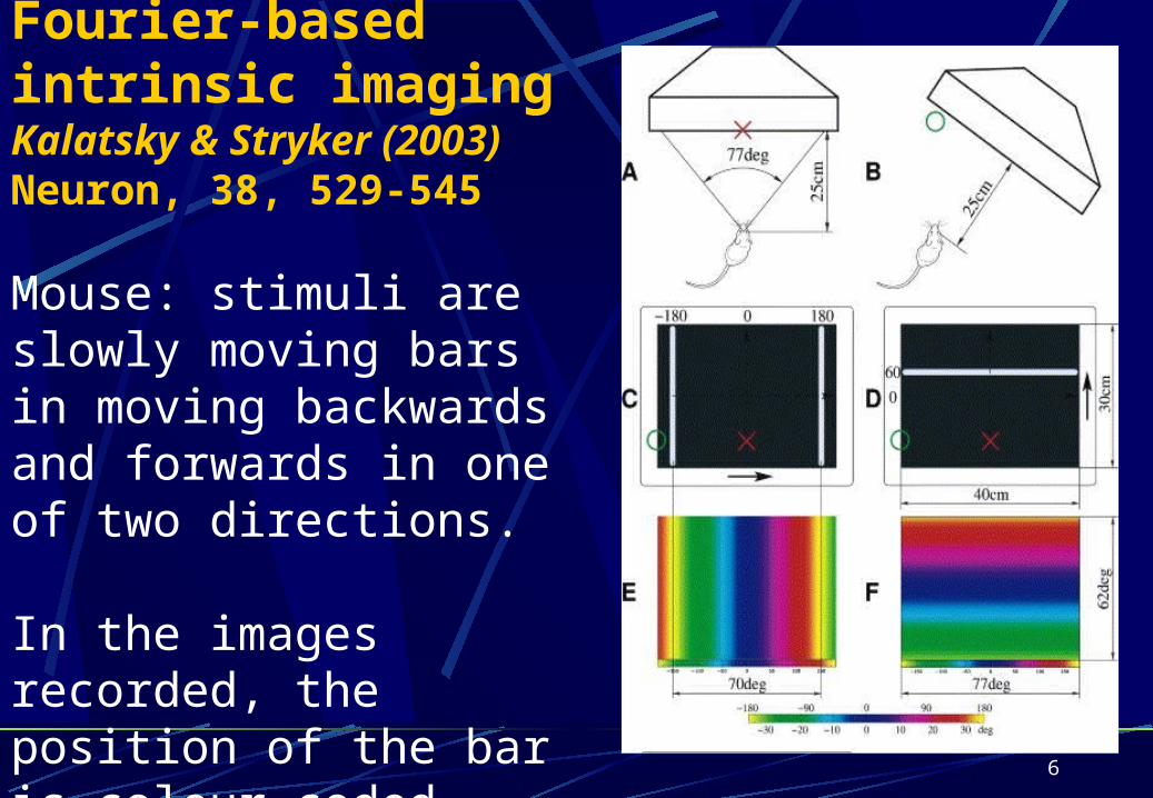
Fourier-based intrinsic imagingKalatsky & Stryker (2003)Neuron, 38, 529-545

Mouse: stimuli are slowly moving bars in moving backwards and forwards in one of two directions.

In the images recorded, the position of the bar is colour coded

7

Fourier-based intrinsic imaging

The local haemodynamic activity generated from a stimulus scanned repeatedly over the visual field is measured continuously

The component of the local response at the stimulus frequency is analysed

For each pixel in the image, the phase at which this component is maximal indicates the corresponding visual field position

8

Kalatsky & Stryker: Recordings from cat/mouse visual cortex

A. Cat: raw signal from a single pixel of an image from visual cortex

B. Cat:

Power spectrum of A.

C. Mouse: Power spectrum

9

Kalatsky & Stryker (2003) A,B: maps recorded from mouse visual cortex

C,D: low resolution map constructed by drawing in 10 degree contours;E,F: comparison with classic data

Problem of response delay resolved by averaging the responses

in the two directions

I now have to convert these coloured maps into point-to-point mappings to enable my

measurement method to be used

10

11

Cang, J. et al. J. Neurosci. 2008;28:11015-11023

Functional retinotopic maps in the mouse superior colliculus

12

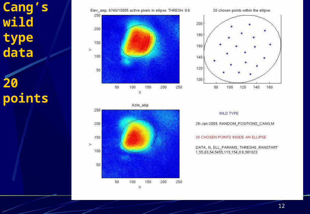
Cang’s wild type data

20 points

13

Wild type, 20 pointsFor each collicular point, find the average field position for the active pixels within a Gaussian distribution of a given halfwidth; this sampling radius is half the mean spacing between adjacent nodes (~180 m)

0 crossingsMean, stddev of length ratios: 1, 0.15

14

By taking the sampling radius as half the spacing of adjacent nodes, effectively the colliculus is being parcellated into 20 distinct areas and the quality of the 20 point map is being measured

0 crossingsMean, stddev of length ratios: 1, 0.15

15

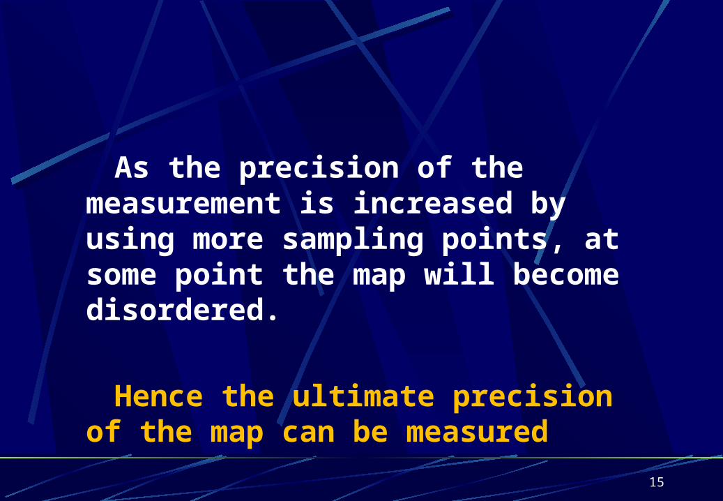
As the precision of the measurement is increased by using more sampling points, at some point the map will become disordered.

Hence the ultimate precision of the map can be measured

16

Wild type, 300 points 5 crossings; length ratio mean, stdev: 1, 0.15

17

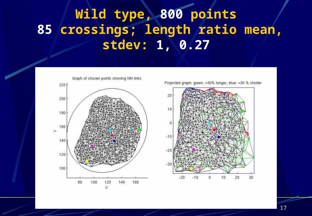
Wild type, 800 points 85 crossings; length ratio mean, stdev: 1, 0.27

Beta2 mutant

20 points

18

19

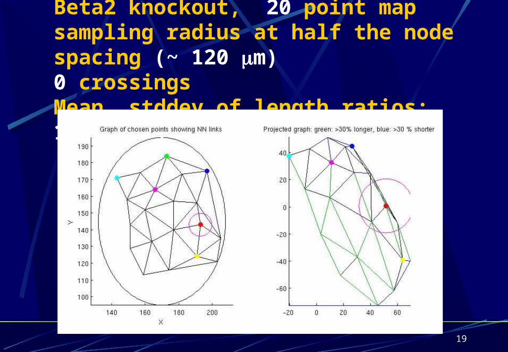
Beta2 knockout, 20 point map sampling radius at half the node spacing (~ 120 m)0 crossingsMean, stddev of length ratios: 1, 0.40

20

Beta2 knockout, 100 points7 crossings; length ratio mean, stdev: 1.1, 0.36

21

Beta2 knockout, 200 points28 crossings; length ratio mean, stdev: 1.1, 0.39

22

Beta2 knockout, 300 points55 crossings; length ratio mean, stdev: 1.2,0.48

23

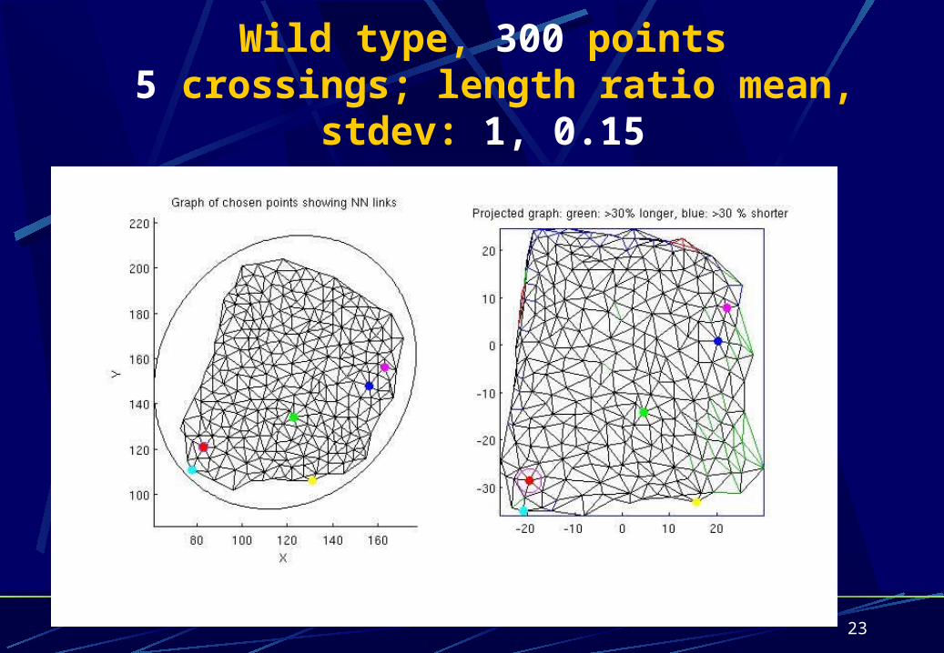
Wild type, 300 points 5 crossings; length ratio mean, stdev: 1, 0.15

A more systematic study, with only the core active region of the

colliculus sampled

24

25

The sampling radius determines the precision of the map calculated

It was set at half the mean distance between collicular nearest-neighbours

Alternatively: specify a constant radius (interpretable as a certain degree of variability in the measurement

process?) and find out how many points are topographically distinguishable

Wild type – crossings as a function of the number of nodes.

Averaged over 8 different starting configurations

26

Wild type data Per cent crossings as a function of the

mean spacing of adjacent nodes

27

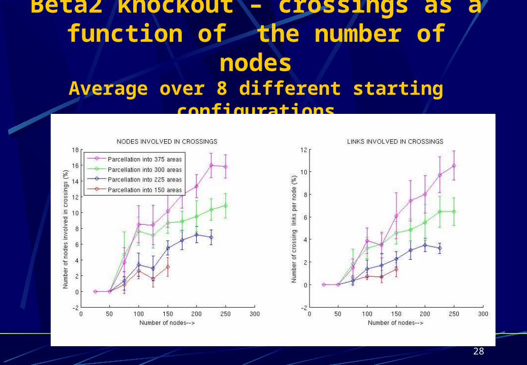
Beta2 knockout – crossings as a function of the number of nodes

Average over 8 different starting configurations

28

Beta2 knockoutPer cent crossings as a function of the

mean spacing of adjacent nodes

29

30

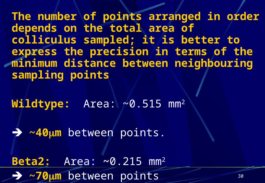
The number of points arranged in order depends on the total area of colliculus sampled; it is better to express the precision in terms of the minimum distance between neighbouring sampling points

Wildtype: Area: ~0.515 mm2

~40m between points.

Beta2: Area: ~0.215 mm2

~70m between points

31

My method of quantifying map order can be applied to these large data sets

Normal maps seem to have quite high precision

I’m able to use the method to compare quantitatively normals with wild type maps

Now to look at other abnormal maps!

In conclusion of Part 2:

32

But aren’t there other well-established methods for this problem?

33

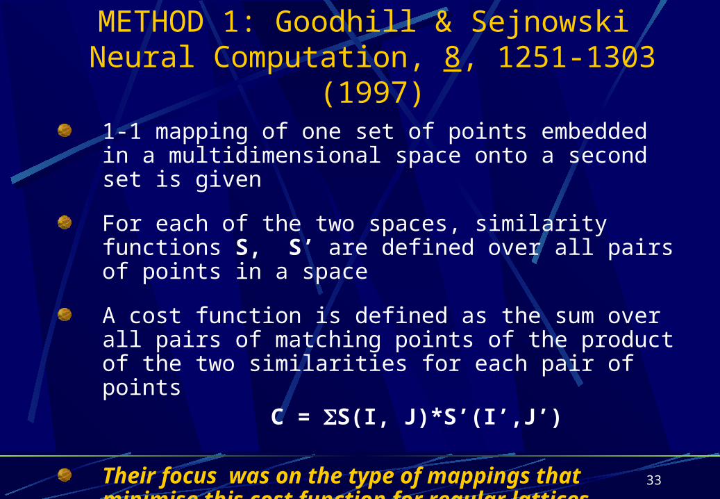
METHOD 1: Goodhill & Sejnowski Neural Computation, 8, 1251-1303 (1997)

1-1 mapping of one set of points embedded in a multidimensional space onto a second set is given

For each of the two spaces, similarity functions S, S’ are defined over all pairs of points in a space

A cost function is defined as the sum over all pairs of matching points of the product of the two similarities for each pair of points

C = S(I, J)*S’(I’,J’)

Their focus was on the type of mappings that minimise this cost function for regular lattices

34

METHOD 2: Procrustes method

This is for comparison of two sets, A and B, of points (‘landmarks’) from a geometric space.

The method involves rotating, translating and rescaling one set, B, to find the best fit, B’, to the points in A.

The measure of best fit is the mean square deviation of the points in A from its corresponding point in B’.

From this can be derived both the best orientation of the map and a measure of the best fit.

35

Comparison of Methods

Goodhill & Sejnowski method is devoted to internal order only, for special cases

Procrustes treats the map as a whole and gives measure of precision assuming an overall orientation of the whole map

The method presented here distinguishes the measure of internal order from that for global order (map orientation)

36

Conclusions of Part 2

In order to be able to distinguish the contributions of different mechanisms to the formation of ordered maps, a reliable method for quantification of maps is needed.

This is the first step towards a quantitative examination of the role of neural activity and molecular cues in setting up ordered retinotopic maps.

37

Part 3

Axonal sorting in other systems:the olfactory system

38

The mouse olfactory system

39

1. Olfactory receptor cell axons in sensory epithelium project to the glomeruli, then to the mitral cells in the olfactory bulb and then to the cerebral cortex

40

Different scale views of olfactory bulb; sensory axons in green, mitral cells in red

41

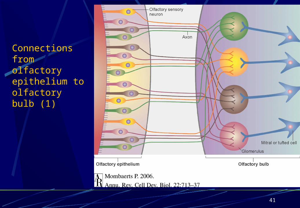
Connections from olfactory epithelium to olfactory bulb (1)

42

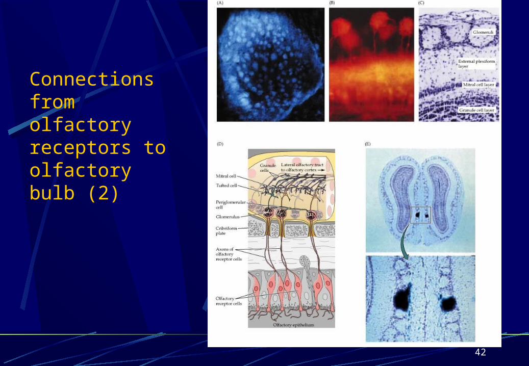
Connections from olfactory receptors to olfactory bulb (2)

43

2. Each of the 10^6 (?) sensory neurons expresses just one of the ~1000 different odorant receptor (OR) genes (?). 3.Neurons expressing the same OR are widely distributed in the olfactory epithelium yet converge to typically 2 out of 1800 glomerular positions in the optic bulb.

44

Differential labelling of the M71 and the M72 genes (ie, genes that encode the M71, M72 receptors) demonstrate this specificity

45

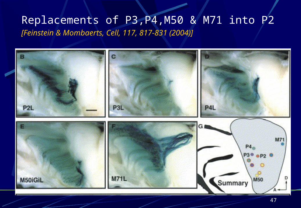
4. Is the position of the projection pattern determined by the target or the receptors?

replacing the gene coding sequence of one OR by that of another causes the glomerular position of the resulting OR axons to shift.

The shift is often to a position between the normal positions of the two ORs

46

Replacement of OR gene M12 with gene P2

[Mombaerts et al,

Cell 87, 675-686 ,1996]

47

Replacements of P3,P4,M50 & M71 into P2 [Feinstein & Mombaerts, Cell, 117, 817-831 (2004)]

48

5. Neurons expressing a given OR exhibit similar levels of ephrinA in their target glomerulus (Cutforth et al, 2004).

Those expressing different ORs express different levels of ephrin-A protein on their axons; there is a 5 fold range of variation over the glomeruli.Over- or under-expression of ephrinA alters the sensory map.

49

Under-expression: Positioning of the glomeruli in

WTs and EphrinA3/A5-/- mutants[Cutforth et al, Cell, 114, 3110312, 2003]

50

What does this all mean? My adaptation of the contextual model for axonal sorting (Feinstein & Mombaerts, 2004):

1. Odorant receptors play an instructive role in the formation of the receptor-specific glomeruli.

1. Initially axons innervate the glomerular area at random.

1. By adjusting their positions through mutual repulsion between axons with different ephrin levels , receptor-specific glomeruli are formed

51

Questions that need answers:

Basic numbers involved? Eg, number of receptors, amount of convergence?Remember that there is continual turnover in olfactory receptorsHow reproducible are the glomeruli patterns from animal to animal? They don’t seem to be entirely random.What information is there about the initial trajectory of axons?What are the current computational models?Or maybe look at Drosophila (see Luo & Flanagan review)?