Embed Size (px)
Citation preview

Modelling, Analysis and Simulation of
Multifrequency Induction Hardening
vorgelegt vonHerrn Dipl.-Math. Thomas Petzold
aus Konigs-Wusterhausen
Von der Fakultat II - Mathematik und Naturwissenschaftender Technischen Universitat Berlin
zur Erlangung des akademischen GradesDoktor der Naturwissenschaften
(Dr. rer. nat.)
genehmigte Dissertation
Promotionsausschuss:
Vorsitzender: Prof. Dr. Wolfgang Konig
Gutachter: Prof. Dr. Dietmar Homberg
Gutachter: Prof. Dr. Alfred Schmidt
Tag der wissenschaftlichen Aussprache: 19.05.2014
Berlin 2014D 83

Impressum:
Copyright: c© 2014 Thomas Petzold
Verlag: epubli GmbH, Berlin, www.epubli.de
Zugl.: Berlin, Technische Universitat, Dissertation, 2014
ISBN 978-3-7375-0087-6

Abstract
For nearly all workpieces made of steel a surface heat treatment to raise the hardnessand the wear resistance is indispensable. A classic method for the heat treatmentis induction hardening, where the heating is done by electromagnetic fields. Dueto the induced eddy currents and the skin effect, the necessary heat to produce thehigh temperature phase austenite is generated directly in the workpiece. During thesubsequent quenching, martensite forms in the boundary layer, which is characterizedby its high hardness. The recently developed concept of multifrequency inductionhardening uses two superimposed alternating currents with different frequencies togenerate a hardening profile following the contour. This method is well suited toharden complex shaped workpieces such as gears, where the coupling distance to theinductor varies. The determination of optimal process parameters requires a lot ofexperience and validation by time-consuming and costly experiments. Therefore, thereis a huge demand for numerical simulations of multifrequency induction hardening.
The present work describes the modelling and the simulation of inductive heatingof workpieces made of steel using the multifrequency concept. The model consistsof a coupled system of partial and ordinary differential equations to determine thetemperature distribution in the workpiece, the electromagnetic fields as the source ofthe Joule heat and the distribution of the high temperature phase austenite, whichprovides information about the resulting hardening pattern. Nonlinearities resultingfrom temperature dependent material parameters and a magnetic permeability thatdepends on the magnetic field itself are of great importance for the performance of thesimulation. The coupled PDE-system is solved by the finite element method, wherebythe electromagnetic subproblem is discretized by curl-conforming edge elements. Sincedue to the skin effect, the boundary layer of the workpiece must be resolved veryaccurately, the grid is generated adaptively using residual based error estimators. Withrespect to the time discretization, the problem represents a multi scale problem. Toobtain a solution of the system, the equations are decoupled by averaging methodsand then solved on the respective time scales.
For a reduced model, where the material parameters depend on the phase fractionof austenite but not on the temperature, the existence of a unique weak solution isestablished.
The developed algorithms are tested and verified for the example of discs with vary-ing diameters. A comparison with experimentally determined surface temperaturesand case depths shows very good correspondence. Further computations for geargeometries are compared to experimental results. For gears hardened with the multi-frequency concept, a very good correspondence between computed phase fractions andexperimentally determined hardening profiles could be observed for cross section cutsas well as for longitudinal cuts through the tip and the root of a tooth. Concludingthe results, the developed software is well suited to predict the expected hardeningprofile.


Zusammenfassung
Fur nahezu alle Bauteile aus Stahl ist eine Oberflachenbehandlung zur Erhohung derHarte und der Verschleißfestigkeit unerlasslich. Als klassisches Verfahren erfolgt beimInduktionsharten die Warmebehandlung mittels elektromagnetischer Felder. Diese er-zeugen aufgrund der induzierten Wirbelstrome und des Skin-Effekts die zur Bildungvon Austenit benotigte Warme direkt im Bauteil. Im anschließenden Abschreckprozessbildet sich in der Randschicht Martensit, welcher sich durch seine hohe Festigkeit aus-zeichnet. Beim relativ neuen Verfahren des Mehrfrequenz-Induktionshartens erzeugenStrome mit unterschiedlichen Frequenzanteilen ein kontourtreues Hartebild. DiesesVerfahren eignet sich sehr gut fur komplexe Bauteilgeometrien wie z. B. Zahnrader,bei denen der Kopplungsabstand zum Induktor variiert. Die Bestimmung optimalerProzessparameter erfordert viel Erfahrung und Validierung mittels zeit- und kostenin-tensiver Experimente. Daher besteht großes Interesse an numerischer Simulation desMehrfrequenz-Induktionshartens.
Die vorliegende Arbeit beschreibt die Modellierung und die Simulation der induk-tiven Erwarmung von Bauteilen aus Stahl mit dem Mehrfrequenzverfahren. Das Mo-dell besteht aus einem gekoppelten System von partiellen und gewohnlichen Differen-tialgleichungen zur Bestimmung der Temperaturverteilung im Werkstuck, der elek-tromagnetischen Felder als Ursache der Erwarmung sowie der Phasenverteilung derHochtemperaturphase Austenit, welche Aufschluss uber das zu erwartende Hartebildgibt. Dabei werden Nichtlinearitaten aufgrund von temperaturabhangigen Materialpa-rametern sowie einer vom Magnetfeld selbst abhangigen magnetischen Permeabilitatberucksichtigt. Die Losung des gekoppelten DGL-Systems erfolgt mit der Methodeder Finiten Elemente, wobei fur das elektromagnetische Teilproblem curl-konformeKantenelemente verwendet werden. Da aufgrund des Skin-Effekts die Randschicht desWerkstucks sehr fein aufzulosen ist, erfolgt eine adaptive Gittergenerierung mittels re-sidualbasierten Fehlerschatzern. Bezuglich der Zeitdiskretisierung stellt das Problemein Mehrskalenproblem dar. Zur Losung des PDE-Systems werden die Gleichungendurch Mittelungsverfahren entkoppelt und auf der jeweiligen Zeitskale gelost.
Fur ein reduziertes Model, bei dem die Materialparameter nur vom Phasenanteil,nicht aber von der Temperatur abhangig sind, werden Aussagen zur Existenz einereindeutigen schwachen Losung hergeleitet.
Die entwickelten Algorithmen werden anhand von Scheiben mit verschiedenenDurchmessern getestet und verifiziert. Ein Vergleich mit experimentell ermitteltenOberflachentemperaturen und Einhartetiefen zeigt sehr gute Ubereinstimmung. Wei-tere Rechnungen fur Zahnradgeometrien werden mit experimentellen Ergebnissen ver-glichen. Auch hier zeigt sich eine sehr gute Ubereinstimmung der berechneten Pha-senverteilungen mit den experimentell ermittelten Hartebildern sowohl im Querschliffals auch in Langsschliffen in Zahnkopf und Zahnfuß fur im Mehrfrequenzverfahrengehartete Zahnrader. Damit eignet sich die entwickelte Software sehr gut zur Vorher-sage des zu erwartenden Harteprofils.

Acknowledgements
The research presented in this thesis was conducted during my work at the Weier-strass Institute of Applied Analysis and Stochastics in the joint research project“MeFreSim” – Modeling, Simulation and Optimization of Multi-Frequency InductionHardening as Part of Modern Production, funded by the German Federal Ministry ofEducation and Research (BMBF). I am grateful to a lot of colleagues who supportedme during this work.
First of all I am obliged to my supervisor, Prof. Dr. Dietmar Homberg, for hissupport during all the years and for giving me the opportunity to work on this researchproject. Furthermore, I want to thank Prof. Dr. Alfred Schmidt for the review of thethesis and the fruitful cooperation within the BMBF research project “MeFreSim” aswell as the coworkers Dr. Oleg Boyarkin, Prof. Dr. Ronald Hoppe, Dr. Qinzhe Liu,Dr. Jonathan Montalvo-Urquizo, Dawid Nadolski and Dr. Alwin Schulz. Moreover,I want to express my gratitude to Dr. Hansjurg Stiele from EFD Induction for hispatient explanations regarding induction hardening and to Prof. Dr. Elisabetta Roccafor her assistance with the mathematical analysis.
Special thanks go to the colleagues at Weierstrass Institute, Prof. Dr. WolfgangDreyer, Anke Giese, Clemens Guhlke, Dr. Daniela Kern, Dr. Oliver Rott and NatalyiaTogobitska. In particular I would like to mention Dr. Robert Huth for his moralsupport and the proofreading of the thesis, Timo Streckenbach and Dr. Wolf Weissfor patiently answering questions regarding pdelib, modelling and everything else.Furthermore, I would like to thank the members of the former Research TrainingGroup “Analysis, Numerics and Optimization of Multiphase Problems”.
Finally, my thanks belong to my family, especially to my wife Kathrin for her sup-port, her patience and her appreciation and to Lisa and Marie, who were motivationand inducement for the work on the thesis and provided balance and distraction atthe same time.


Contents
1. Introduction 1
2. Physical background 72.1. Phase transitions in steel . . . . . . . . . . . . . . . . . . . . . . . . . . 7
2.1.1. Phases in steel . . . . . . . . . . . . . . . . . . . . . . . . . . . . 72.1.2. The austenite to ferrite phase transformation . . . . . . . . . . . 92.1.3. The formation of pearlite . . . . . . . . . . . . . . . . . . . . . . 102.1.4. The formation of martensite . . . . . . . . . . . . . . . . . . . . . 112.1.5. TTT-diagrams . . . . . . . . . . . . . . . . . . . . . . . . . . . . 11
2.2. The concept of multifrequency induction hardening . . . . . . . . . . . . 132.2.1. Description of induction hardening . . . . . . . . . . . . . . . . . 132.2.2. Multifrequency induction hardening . . . . . . . . . . . . . . . . 14
3. The model 193.1. Electromagnetic effects . . . . . . . . . . . . . . . . . . . . . . . . . . . . 20
3.1.1. Maxwell’s equations in differential form . . . . . . . . . . . . . . 203.1.2. Interface- and boundary conditions . . . . . . . . . . . . . . . . . 213.1.3. Magnetic vector- and electric scalar potential . . . . . . . . . . . 233.1.4. Characterization of electric sources . . . . . . . . . . . . . . . . . 24
3.2. Phase fraction of austenite . . . . . . . . . . . . . . . . . . . . . . . . . . 263.3. Balance of energy . . . . . . . . . . . . . . . . . . . . . . . . . . . . . . . 273.4. Characterization of the material parameters . . . . . . . . . . . . . . . . 293.5. Summary of the model . . . . . . . . . . . . . . . . . . . . . . . . . . . . 30
4. Analysis of a simplified model 334.1. Notation and preliminary assumptions . . . . . . . . . . . . . . . . . . . 334.2. Hypotheses . . . . . . . . . . . . . . . . . . . . . . . . . . . . . . . . . . 364.3. Weak formulation and main theorem . . . . . . . . . . . . . . . . . . . . 374.4. Proof of the existence result . . . . . . . . . . . . . . . . . . . . . . . . . 38
4.4.1. Existence of a (local in time) solution . . . . . . . . . . . . . . . 384.4.2. Global a priori estimates . . . . . . . . . . . . . . . . . . . . . . . 414.4.3. Stability estimate . . . . . . . . . . . . . . . . . . . . . . . . . . . 45
5. Numerical solution of the induction hardening problem 495.1. Discretization in space by the Galerkin method . . . . . . . . . . . . . . 50
5.1.1. Introduction of the Galerkin method . . . . . . . . . . . . . . . . 505.1.2. The semi-discretized problem . . . . . . . . . . . . . . . . . . . . 52
ix

x Contents
5.2. An overview of the finite element method . . . . . . . . . . . . . . . . . 545.2.1. The spatial decomposition of the computational domain . . . . . 555.2.2. An abstract definition of a finite element . . . . . . . . . . . . . . 555.2.3. Finite elements for H1 . . . . . . . . . . . . . . . . . . . . . . . . 585.2.4. Finite elements for H(curl) . . . . . . . . . . . . . . . . . . . . . 595.2.5. About the spatial discretization of the phase fraction . . . . . . . 62
5.3. Discretization in time and nonlinear behaviour . . . . . . . . . . . . . . 635.3.1. Discretization in time . . . . . . . . . . . . . . . . . . . . . . . . 635.3.2. Nonlinearities . . . . . . . . . . . . . . . . . . . . . . . . . . . . . 645.3.3. Different time scales for heat diffusion and electromagnetic effects 665.3.4. Time discretization of the coupled system . . . . . . . . . . . . . 685.3.5. On the existence of solutions for the discretized system . . . . . 705.3.6. Solution of the linearized systems . . . . . . . . . . . . . . . . . . 71
5.4. Adaptive mesh generation . . . . . . . . . . . . . . . . . . . . . . . . . . 735.4.1. A general adaptive algorithm . . . . . . . . . . . . . . . . . . . . 745.4.2. A residual based error estimator for Maxwell’s equation . . . . . 755.4.3. Strategies for the grid refinement . . . . . . . . . . . . . . . . . . 79
5.5. Averaging of the magnetic permeability . . . . . . . . . . . . . . . . . . 815.6. The complete algorithm to solve the induction hardening problem . . . 83
6. Simulation 856.1. Test of the adaptive grid refinement . . . . . . . . . . . . . . . . . . . . 856.2. Numerical simulations for discs . . . . . . . . . . . . . . . . . . . . . . . 87
6.2.1. Numerical simulations . . . . . . . . . . . . . . . . . . . . . . . . 876.2.2. Experimental setup . . . . . . . . . . . . . . . . . . . . . . . . . . 926.2.3. Experimental verification and discussion . . . . . . . . . . . . . . 94
6.3. Numerical simulations for gears . . . . . . . . . . . . . . . . . . . . . . . 966.3.1. Numerical simulation . . . . . . . . . . . . . . . . . . . . . . . . 966.3.2. Experimental verification . . . . . . . . . . . . . . . . . . . . . . 1026.3.3. Contour hardening of gears in an industrial setting . . . . . . . . 1046.3.4. Discussion . . . . . . . . . . . . . . . . . . . . . . . . . . . . . . . 106
7. Conclusion and Outlook 109
A. Appendix 113A.1. Integral identities . . . . . . . . . . . . . . . . . . . . . . . . . . . . . . . 113A.2. Material parameters for the steel 42CrMo4 . . . . . . . . . . . . . . . . 114
A.2.1. Specific heat capacity . . . . . . . . . . . . . . . . . . . . . . . . 114A.2.2. Heat conductivity . . . . . . . . . . . . . . . . . . . . . . . . . . 114A.2.3. Electrical conductivity . . . . . . . . . . . . . . . . . . . . . . . . 114A.2.4. Magnetic permeability . . . . . . . . . . . . . . . . . . . . . . . . 115A.2.5. Further parameters . . . . . . . . . . . . . . . . . . . . . . . . . . 116
A.3. Averaging of the Joule heat . . . . . . . . . . . . . . . . . . . . . . . . . 116

Chapter 1.
Introduction
For nearly all workpieces made of steel a surface heat treatment to raise the hardnessand the wear resistance is indispensable. A classic method for the heat treatment ofsteel is induction hardening, where the heating is done by electromagnetic fields. Dueto the induced eddy currents and the skin effect, the necessary heat to produce thehigh temperature phase austenite is generated directly in the workpiece. During thesubsequent quenching, martensite forms in the boundary layer, which is characterizedby its high hardness. Induction heating is a very fast and energy efficient process, sincethe heat is generated directly in the workpiece. Furthermore, in industrial applications,it can be integrated directly into the process chain. But due to the skin effect a contourhardening for gears is hardly possible using only a single frequency.
The recently developed concept of multifrequency induction hardening uses twosuperimposed alternating currents with different frequencies to generate a hardeningprofile following the contour. This method is well suited to harden complex workpiecessuch as gears, where the coupling distance to the inductor varies.
The determination of optimal process parameters requires a lot of experience andvalidation by time-consuming and costly experiments. Therefore, there is a huge de-mand for numerical simulations of multifrequency induction hardening. Though nu-merical simulations in 2D are commonly used by engineers, these can not reproducecomplex shaped workpieces and inductor geometries. Especially at corners of work-pieces a partial melting occurs first. This can only be resolved by 3D simulations. Thecomputational time represents the biggest restriction in the professional application ofsimulation tools. In addition, there is only an insufficient support for complex 3D sim-ulations in commercial software tools. Therefore, it is the aim of this thesis to developan effective 3D simulation tool for multifrequency induction hardening of gears.
The main challenges for the design of a simulation tool for the multifrequency in-duction hardening process can be summarized as follows. For a correct reproduction ofexperimental results, the consideration of nonlinear material parameters is inevitable.In addition to temperature dependent material parameters, the magnetic permeabilitydepends on the magnetic field itself, resulting from the magnetic saturation behaviour.These nonlinearities as well as the supply of a multifrequency inductor current gener-ated by transistorized power converters require the solution of the model equations inthe time domain instead of the easier to handle frequency domain. From an analyticalpoint of view, the analysis of strongly coupled, nonlinear systems of partial differentialequations resulting from the modelling of real world phenomena is always a challenge.
1

2 1. INTRODUCTION
To make things worse, the coupled, nonlinear system represents a multiscale problemin time, since the typical time scales for heat conduction and electromagnetic processesdiffer by orders of magnitudes. In addition, due to the skin effect, different lengthscales must be considered as well. Compared to the overall workpiece dimensions, theinduced eddy current density concentrates in a small boundary layer, which must beresolved by the space discretization. Therefore, the numerical solution requires theuse of graduated grids, which can be generated adaptively.
While the modelling and the numerical simulation of induction hardening for axissymmetric workpieces in 2D is standard in commercial software, the effective simula-tion of the coupled system in 3D is a challenge itself. In 3D, the spatial discretizationof Maxwell’s equations requires the use of suitable methods, e. g. the finite elementmethod using so-called edge elements.
The simulation of induction hardening gains much interest in the literature. In thefollowing, an overview of the state of research regarding the modelling, analysis andthe simulation of induction hardening is given. There are numerous articles regardingthe simulation of induction hardening using a single frequency. In most cases, axialsymmetric parts are considered. The simulations are usually done in the frequencydomain, e. g. [16, 43]. The latter one considers the induction hardening of axial sym-metric parts using a mixed finite element and boundary element method to solve theelectromagnetic problem. A model combining electromagnetic, thermal and mechani-cal phenomena for axisymmetric induction heating processes is for example consideredin [6]. Often, commercial software packages are used, e. g. [52], where a numerical andexperimental study of the induction heat treatment of steel bars is carried out.
New requirements for numerical simulations appeared with the development of themultifrequency concept, [53]. There, multiple currents with frequencies that differ bymore than a power of ten are supplied to one common inductor coil. With this conceptit is possible to obtain a surface hardened region that follows the contour of complexshaped workpieces such as gears.
Finite element simulations in 3D using the multifrequency approach are done byWrona [85]. There, the system is solved in the frequency domain using commercialfinite element software. Since the software does not support the use of multiple fre-quencies directly, the different frequency powers are computed stepwise and separatelyat different time steps on a fixed grid. The stepwise calculation results in an oscil-latory behaviour of the temperature, which is not desirable and the consideration ofthe equations in the frequency domain allows only the use of a constant magneticpermeability. In the present thesis, the consideration of nonlinear material data, espe-cially the nonlinear magnetization curve, is essential to reproduce the experimentallyobtained hardening profiles.
In order to judge the expected hardening profile, isothermal lines for the transfor-mation temperature are compared to experimental hardening results. Phase transitionkinetics are not considered. This can produce misleading results, since due to the ex-tremely short heating times, a shift of the transformation temperature can occur andin addition, heat conduction effects after switching off the inductive heating mightaffect the transformed phase fraction.

3
A recent work considers the complete process of multifrequency induction harden-ing including the quenching stage and the computation of internal stresses, [72]. Thecomputations are carried out in 2D for radial symmetric parts such as shafts. Themagnetic field is computed in the frequency domain. Adaptive grid generation is notconsidered. An experimental validation shows good agreement with computationalresults in the case of multifrequency induction hardening, but only for radial symmet-ric workpieces. 3D simulations for multifrequency induction hardening of gears areconsidered in [68]. The magnetic saturation behaviour is taken into account by aniteration procedure, which results in a high increase of computational time.
For the analysis of induction heating problems there are results for the situation ofJoule heating that consider the equations in the simpler frequency domain, [23, 31].The equations in the time domain are considered in [38], where existence of a weaksolution is shown, and in [40], where a stability estimate is given for the situation ofconstant material parameters.
Regarding the numerical solution of the induction hardening problem, adaptive fi-nite element methods and corresponding error estimates are state of mathematicaltechnology for the single components of the model such as heat conduction phenom-ena [69, 83, 88], and computational electromagnetics [7, 15, 70], only to mention some.We use these techniques to create adaptive grids that resolve the eddy current regionwith sufficient accuracy.
For solving Maxwell’s equations by the finite element method, edge elements ofNedelec type are quite popular, [57, 58]. Based on this fundamental work, higherorder methods were developed in the recent years [71, 86], introducing hierarchicalfinite element basis functions. Typically, the equations are considered in the frequencydomain, which has limitations regarding nonlinear problems. In [3, 4] the so-called mul-tiharmonic approach is investigated, which allows the solution of nonlinear problemsin the frequency domain by considering truncated Fourier-expansions. If N denotesthe number of Fourier coefficients, the advantage of avoiding a time-stepping schemeis compensated by an increase in dimension by a factor of 2N . In addition, in the caseof nonlinear problems, the resulting linear system for the Fourier coefficients is fullycoupled. An efficient algorithm to solve linear systems of equations is the multigridmethod [37]. The application of multigrid methods to induction heating problems isconsidered e. g. in [41]. Though the performance is indisputable, the implementationof these methods is quite involved.
The subject of this thesis is the modelling, the analysis and the simulation of mul-tifrequency induction hardening in 3D. Using modern mathematical techniques, it isthe aim to develop a high performance simulation tool, which is able to predict thehardening pattern with high accuracy. With the availability of effective algorithms,the numerical simulation of the process is not only a supplement, but can even becomea replacement for time consuming experiments, such that the effectivity of multifre-quency induction hardening as a cost- and energy efficient alternative to classic casehardening by carburization can be further increased.
The main contributions of this thesis are the following. A model is derived thatreflects the different physical aspects of the induction hardening process. The tem-

4 1. INTRODUCTION
perature evolution is determined by heat conduction effects, whereby the heat sourceis realized by electromagnetic fields. The phase transition kinetics to determine theexpected hardening profile is modelled by rate laws that are based on experimentalmeasurements.
For a realistic description, the consideration of nonlinear material parameters, espe-cially the nonlinear magnetization curve, is essential. Furthermore, due to the arisingnonlinearities and the periodic, but not necessarily harmonic source currents, the elec-tromagnetic fields are considered in the time domain.
Regarding the respective model components, analytical results regarding the exis-tence and uniqueness of solutions are known. For coupled, nonlinear PDE systems,these represent a challenge. Due to the high complexity, analytical investigations fora reduced model are considered, where the material parameters depend on the phasefraction but not on the temperature. The existence of a unique weak solution is es-tablished.
The numerical simulation is considered for the full nonlinear model. For the solutionof the coupled system of partial differential equations in 3D the finite element methodis applied, where for the electromagnetic subproblem curl-conforming finite elementsare implemented. The efficient algorithmic realization is of great significance. Withthe mathematical optimization of the process in mind, where a repeated solution ofthe equations is necessary, the computational time is an important factor. For thesimulation, modern mathematical techniques such as adaptivity and parallelizationare utilized in order to account for the demands of a modern simulation software forthe contour hardening of complex shaped workpieces.
The experimental verification of the simulation results for the inductive heating ofdiscs and gears confirms the good performance of the solution algorithm. It is possibleto resolve the contour hardened boundary layer for gears, where in addition to theprofile in the cross section of the tooth also the lateral profile in the tip and the rootof a tooth is reproduced.
The thesis is organized as follows. In the next chapter, we introduce the physicalbackground. We describe the different phases in steel and the occurring phase tran-sition mechanisms. Furthermore, a description of multifrequency induction hardeningis given.
Chapter 3 is devoted to the modelling of the process. The equations describingthe electromagnetic phenomena, the heat conduction effects and the transformationkinetics for the formation of the high temperature phase austenite are derived. Fur-thermore, thermodynamic consistency of the model is shown by applying the secondlaw of thermodynamics.
In Chapter 4 the existence and uniqueness of solutions for a simplified model isinvestigated, where the material parameters depend only on space and the volumefraction of austenite, but are independent of the temperature.
The main part of the thesis is devoted to the numerical simulation of the inductionheating process, see Chapter 5. The finite element method to solve the system of partialdifferential equations is introduced. The different aspects arising from nonlinearities,different time scales and other physical properties of the process, which need to be

5
considered in the simulation, are addressed and the overall algorithm to solve theinduction hardening problem is given.
Finally, numerical simulations for disc and gear geometries are presented. The re-sults are compared to experiments that were conducted by Institut fur Werkstofftech-nik (IWT), Bremen and EFD Induction, Freiburg. A summary of the thesis and anoutlook for further developments is given in Chapter 7. In an Appendix, supplemen-tary material and the material data used in the simulations is presented.


Chapter 2.
Physical background
Introduction
In general, the aim of any surface hardening process is to transform the boundarylayer to a martensitic microstructure, which is characterized by an increased hardness.This improves the wear resistance. The essential feature is to create the martensiticstructure only within a given depth, leaving the remaining part of the workpiece in itsinitial microstructure to reduce the chance of cracks by fatigue effects. The principalprocedure for any surface hardening consists of the following steps:
(i) Heating of the workpiece, respectively the surface area to the required austeni-tization temperature,
(ii) holding of the process temperature in order to ensure a complete austenitization,
(iii) rapid cooling to room temperature such that the hard phase martensite forms.
Knowledge of the different phases in steel and the occurring phase transition mech-anisms is necessary to understand the process of induction hardening. In the nextsection, the different phases in steel are introduced. Then, the process of inductionhardening using the multifrequency concept is explained.
2.1. Phase transitions in steel
2.1.1. Phases in steel
Steel mainly consists of iron and carbon. Industrial steels contain a large number offurther alloying elements such as chromium, manganese, silicon or nickel that affectthe properties and hardness of the steel but the most important alloying element iscarbon.
We start with the description of pure iron. Pure iron is very soft and ductile.Therefore, it is not used as construction material. But due to the high magneticpermeability it is an important material in electronics. The cooling and heating curveof pure iron is depicted in Figure 2.1. Below the melting temperature of 1536 C ironcrystalizes as δ-iron with a body centred cubic structure (bcc). On further cooling,the iron transforms into the face centred cubic γ-iron at a temperature of 1392 C.This modification and also the solid solutions with an fcc-crystal structure in steel aredenoted as austenite. At a temperature of 906 C, the point Ar3, the iron transforms
7

8 2. PHYSICAL BACKGROUND
400
600
800
1,000
1,200
1,400
1,600melting temp. θS = 1536 C
Ar4 = 1392 C
Ar3 = 906 C
Ar2 = 769 C
Ac4
Ac3 = 911 C
Ac2
δ-Fe (bcc)
γ-Fe (fcc)
α-Fe (bcc)
time t →
tem
per
atu
reθ
[C
]
CoolingHeating
Figure 2.1.: Cooling and heating curve of pure iron, adapted from [5]
again into a bcc crystal, the α-iron. This structure and also the corresponding phase insteel, which is stable at room temperature, are denoted as ferrite, [5]. The two latticestructures, bcc and fcc, are depicted in Figure 2.2. The fourth holding point (Ar2) at
Figure 2.2.: BCC- and FCC-unit cell of ferrite and austenite
a temperature of 769 C is denoted as the Curie-temperature. This point is not relatedto a lattice transformation. At the Curie-temperature the magnetic properties changefrom paramagnetic at high temperatures to ferromagnetic. As indicated in Figure2.1, the temperatures at which the phase transition occur can be different for heatingand cooling (thermal hysteresis). Therefore, one has to clearly distinguish betweenthe holding points on heating, denoted by Ac (arret chauffage) and cooling, Ar (arretrefroidissement). The effect of thermal hysteresis increases with an increase of theheating and cooling rates. Especially in induction hardening very high heating and

2.1. Phase transitions in steel 9
cooling rates occur. This influences the temperatures at which the phase transitionstake place. In addition, the effect of thermal hysteresis increases with the addition ofalloying elements.
There are two different possibilities to dissolve alloying elements, either as substitu-tional or interstitial solid solution. Usually, metallic alloying elements such as nickel,chromium, manganese and many others are dissolved as substitutional solution, thealloy atoms replace an iron atom in the corresponding bcc- or fcc-lattice. The latticestructure stays the same.
This is different for carbon. Carbon is dissolved on interstitial lattice sites and formsan interstitial solution. The bcc- and fcc-iron crystals form interstitial lattices consist-ing of tetrahedral and octahedral sub-lattice sites. Carbon is dissolved on octahedrallattice sites. These are smaller than the atomic diameter of carbon, which results in adistortion of the parent bcc- or fcc-lattice, see also Table 2.1. This distortion is even
size of interstices size ratio interstices/carbon atom
octahedral site bcc 0.154 · rFe 25.6 %
tetrahedral site bcc 0.291 · rFe 48.5 %
octahedral site fcc 0.41 · rFe 68.3 %
Table 2.1.: Sizes of interstices in bcc- and fcc-iron (rFe = 1.28 A, rC = 0.77 A, diameterof iron/carbon atom)
larger for the bcc-lattice, which results in different maximum solubilities of carbon inferrite and austenite. The maximum solubility of carbon in γ-iron is 2 % per masswhile in α-iron it is only 0.02 %. Despite the larger diameter of the tetrahedral sub-lattice site in bcc-iron, carbon is dissolved on octahedral sites since a dissolved carbonatom on tetrahedral interstices causes a larger lattice deformation, cf. [5].
Alloying elements, especially carbon, have a huge influence on the lattice trans-formation from fcc to bcc and consequently on the phase transition kinetics. In thefollowing, the most important phase transformation mechanisms in steel are described.
2.1.2. The austenite to ferrite phase transformation
In steel, one distinguishes between reconstructive and displacive transformations, [10].An example for the latter one is the formation of martensite by rapid quenching, seeSection 2.1.4, while the decomposition of austenite into ferrite at high temperaturescan be characterized as reconstructive transformation. The movement of atoms isthermally activated. Therefore, diffusion effects are significant at high temperaturesand control the phase transition from austenite to ferrite.
When cooling the steel below the Ar3-temperature, it is more favourable from anenergetic point of view that the iron atoms arrange in a bcc-crystal instead of thefcc-structure of austenite. This process usually starts by nucleation of an α-nucleusat an austenitic grain boundary. Since the carbon solubility in ferrite is much smallerthan in austenite, carbon has to diffuse into the parent austenite and is accumulated

10 2. PHYSICAL BACKGROUND
at the α/γ-interface. The iron atoms are able to cross the interface immediately andchange their crystallographic orientation. The ferrite nucleus grows by movement ofthe α/γ-interface at the expense of the austenite. If the atoms are attached to theferrite nucleus randomly, the interface can propagate readily in all directions, [24].The excess carbon that accumulates at the interface forms a barrier for further carbonatoms that are rejected from the ferrite. The pile up of carbon at the interface hasto be balanced by diffusion. Therefore, the carbon diffusion determines the kineticsof the phase transition process. At high temperatures, the movement is rapid, whilea reduction in temperature lowers the mobility of the atoms and consequently thevelocity of the transformation front.
If the carbon concentration in austenite is too high such that it can not be balancedby diffusion, the carbon enriched compound cementite precipitates from the parentaustenite. At the eutectoid concentration of 0.8 %, ferrite and cementite crystallize byan alternating process and pearlite forms.
2.1.3. The formation of pearlite
Pearlite is a lamellar mixture of the phases ferrite and the metastable compound ce-mentite with the structural formula Fe3C. The first step of the formation of pearlite isthe nucleation of one of the components, either ferrite or cementite at grain boundariesof the parent austenite. Though the formation of pearlite has been described in con-siderably detail in the literature and is subject of many investigations, some aspectsare still not fully understood. One of them is e. g. the role of the active nucleus, [87].The following description of the formation of pearlite follows [63].
It is assumed that cementite is the active nucleus. Since cementite has a highcarbon concentration (6.66 %), the surrounding of the nucleus depletes in carbon,which favours the formation of ferrite. Ferrite forms adjacent to the cementite andcarbon is rejected into the austenite matrix. The enrichment in carbon favours theformation of cementite. This process repeats and the pearlite colony grows sidewisealong the grain boundary.
In addition to the sidewise growth, the colony also grows edgewise into the austenitegrain. The rate of the edgewise growth is controlled by the diffusion of carbon from thetips of the ferrite lamella to the tips of the cementite lamella. Therefore, the diffusionof the rejected carbon through the austenite affects the morphology of pearlite. Athigher undercooling the mobility of the carbon atoms is more and more limited, whichresults in a smaller distance of the lamellas and therefore a finer structure of pearlite.
If the alloy composition does not correspond to the eutectoid composition of 0.8 %first, ferrite or cementite nucleates and covers the grain boundaries as pro-eutectoidferrite (in hypoeutectoid steel) or pro-eutectoid cementite (in hypereutectoid steel)until the remaining parental austenite reaches the composition of 0.8 %. Then, thetransformation takes place as described above.

2.1. Phase transitions in steel 11
2.1.4. The formation of martensite
Martensite forms by a diffusionless phase transformation from the austenite in the caseof rapid cooling below the martensite start temperature Ms. Due to the rapid cooling,diffusion processes are suppressed, the transformation is characterized as displacive andhappens by a diffusionless shear transformation of the iron lattice. The iron atomsmove only marginal by a fraction of the atomic diameter. The carbon atoms, whichare dissolved in the fcc-crystal of austenite, are forced to their interstitial sites. Thisresults in a supersaturated, tetragonal distorted bcc-lattice. These lattice distortionsare the reason for the high hardness of martensite.
The fraction of martensite zα′ that is produced can be estimated by the equation ofKoistinen and Marburger, [47]
1− zα′ = exp(−β(Ms − θ)),
where β > 0 is a parameter to be determined by experiments and θ denotes the quenchtemperature. As one can see, there is no time dependence in the equation above. Themartensite formation is considered as a-thermal due to a very rapid nucleation andgrowth. Therefore, the time dependence can be ignored. The driving force is theundercooling below the martensite start temperature Ms. There is always a fractionof retained austenite, which can also be estimated by the relation above, it correspondsto the fraction 1− zα′ .
The temperature at which no more martensite forms on further cooling is denotedas the martensite finish temperature, Mf . In the relation above, there is no martensitefinish temperature, in applications it is defined as the temperature that correspondsto a martensite fraction of zα′ = 0.95.
In order to produce as much martensite as possible, a rapid cooling is necessary.The cooling rate, at which no additional phases such as ferrite, pearlite or bainiteare produced, is called the critical cooling rate. The martensite start and finish tem-peratures Ms and Mf as well as the critical cooling rate depend essentially on thealloying elements and the carbon content. They are different for the various types ofsteel. Therefore, not every steel is suitable to produce high amounts of martensite andconsequently not suitable for induction hardening.
In the past decades further approaches to describe the formation of martensite weredeveloped. We refer to [80] for a survey and a comparison of different model equationsto describe the temporal evolution of martensite.
2.1.5. TTT-diagrams
The microstructure and the distribution of the different phases such as ferrite, pearliteor martensite is crucial for the mechanical properties of the steel. An importanttool characterizing the temperature and carbon-concentration dependent state of thephases is the iron-carbon phase diagram. It shows the stable phases at a given tem-perature and a given mean carbon concentration and provides insight in the occurringphase transitions. With the help of the iron-carbon diagram it is for example possibleto determine the carbon concentration and the volume fraction of the pure phases in a

12 2. PHYSICAL BACKGROUND
phase mixture using the so called lever rule, cf. [34]. Unfortunately, the diagram pro-vides no information on the transformation rates, the distribution of the phases or themicrostructure. The validity of the phase diagram is limited to processes that occurat conditions close to equilibrium, i. e. at extremely slow cooling rates, and involve nomechanical effects or the occurrence of phase like martensite, which develop throughdisplacive transformations far from diffusional equilibrium.
Most of the steels used in practical applications contain in addition to carbon furtheralloying elements such as chromium, manganese, silicon or nickel. These substitutionalalloying elements have a huge influence on the material properties. The temperature atwhich a phase transition occurs can change or even the occurrence of a phase is skippedat all. This is also not reflected in the iron-carbon diagram and its application islimited. Further tools are required to describe the temporal transformation behaviourof the formation of pearlite or the formation of martensite.
The temporal transformation process involves nucleation and growth and is conven-tionally represented by time-temperature-transformation (TTT)-diagrams. The degreeof transformation is indicated over time, usually on a logarithmic scale. These dia-grams must be interpreted exclusively at constant temperatures. The determination ofthese diagrams is carried out by isothermal experiments for a multitude of specimensof a single type of steel in order to determine the time that is necessary to obtain agiven pearlitic fraction. This diagram is then valid only for the specific steel with thecorresponding composition.
Isothermal transformations have in general only little relevance for industrial ap-plications. Usually in the manufacturing process, the temperature is not constant.The transformation kinetics under non-isothermal conditions is depicted in continuouscooling transformation (CCT)-diagrams. There, the state of the phase transition isindicated along given cooling profiles, see Figure 2.3. The different lines indicate thebeginning and the end of the transformation along the temperature curve for a givencooling rate. In addition, the martensite start and finish temperatures are indicatedand the critical cooling rate, at which only martensite forms, can be obtained. Theknowledge of the critical cooling rate is essential for the induction hardening process,since the formation of any undesired phase such as ferrite, pearlite or bainite duringthe quenching, must be suppressed. On the other hand, the cooling rate is restricted bytechnical limitations and the critical cooling rate is an indicator if the steel is suitablefor induction hardening.
The reverse process, the formation of austenite from a ferritic and pearlitic matrixduring the heating is represented by time-temperature austenitization (TTA)-diagrams,see Figure 2.4. Due to the thermal hysteresis, the Ac3 temperature at which austeniteforms is shifted to higher temperatures with increasing heating rate. This has tobe taken into account in the induction heating process with its short heating times.It is necessary to heat the specimen to higher temperatures to achieve a completeaustenitization.

2.2. The concept of multifrequency induction hardening 13
Figure 2.3.: Continuous cooling diagram for the steel 42CrMo4, [84]
2.2. The concept of multifrequency induction hardening
2.2.1. Description of induction hardening
In induction hardening as a method for the heat treatment of steel, the necessaryheat to transform the boundary layer to austenite is generated by induced electriccurrents. The principle is the following. A coil that is connected to an alternatingcurrent source (converter) generates a periodically changing electromagnetic field. Thetemporal changing magnetic flux induces a current in the workpiece that is enclosedby the induction coil. Due to the resistance of the workpiece, some part of the poweris transformed into eddy current losses and a heating of the workpiece results (Jouleheating).
The induced current itself generates a magnetic field, which opposes the inductorcurrent. The electric fields superimpose each other. This results in a decrease ofthe magnetic field and consequently of the electric field in radial direction. As aconsequence, the eddy currents are concentrated in the surface layer of the workpiece.This is called the skin effect.
The penetration or skin depth of the electric current is defined as the depth δ atwhich the current density reduces to 37% of its maximum value, [8]. The penetrationdepth depends on the electric and magnetic properties of the workpiece, but mainly onthe frequency of the alternating current. Simplified, there holds the following relation

14 2. PHYSICAL BACKGROUND
Figure 2.4.: Time-temperature-austenitization diagram for the steel 42CrMo4, [59]
δ =1√πσµf
, (2.1)
where σ [A mm2/Vm] denotes the electric conductivity, µ [Vs/Am] the magnetic per-meability and f [1/s] the frequency. One has to note that the material parametersare temperature dependent. Consequently, the penetration depth changes during theheating. In addition, the relative permeability depends on the magnetic field intensity.However, the frequency is the most significant parameter to control the penetrationdepth, see also Figure 2.5, where the penetration depth is depicted for different tem-peratures and materials.
2.2.2. Multifrequency induction hardening
Since the penetration depth depends on the frequency of the inductor current, it isdifficult to obtain a uniform contour hardened surface area for complex workpiecegeometries such as gears using a current with only one fixed frequency. If for example,a high frequency (HF) is applied, then the penetration depth is small and it is possibleto harden only the tip of the tooth. With a medium frequency (MF) it is possible to

2.2. The concept of multifrequency induction hardening 15
101 102 103 104 105 106 107
10−2
10−1
100
101
102
frequency [Hz]
pen
etra
tion
dep
thδ
[mm
]steel, 1000 C, µr = 1, σ = 0.83
stainless steel, 20 C, µr = 1, σ = 1.25steel, 400 C, µr = 30, σ = 2.22steel, 20 C, µr = 100, σ = 7.69
Figure 2.5.: Penetration depth δ in dependence on the frequency of the inductor cur-rent, [51]
heat the root of the tooth, but not the tip. With a single frequency, a hardening ofthe whole tooth can only be achieved by increasing the heating time. But then, thecomplete tooth is heated beyond the austenitization temperature, which results in acomplete martensitic structure of the tooth after quenching. This is also not desirable,since the chance of material failure increases.
The recently developed approach is to supply both frequency powers simultaneously.This concept is called multifrequency induction hardening, see also Figure 2.6. In order
∼ ≈∼+≈
Figure 2.6.: The effect of medium-, high- and multifrequency induction heating; MF(left): only the root of the tooth is heated, HF (middle): only the tip ofthe tooth is heated, MF+HF (right): tip and root of the tooth are heated(adapted from [73])
to achieve a hardening profile that follows the contour of the gear, very short heatingtimes are necessary in order to avoid heat diffusion into the workpiece. In the past,multifrequency hardening was performed by subsequent heating of gearwheels in twoseparate inductors that are fed by power supplies with different frequencies. With
16 2. PHYSICAL BACKGROUND
short heating times of below 500 ms [62], which is typical for the application to gears,the transfer of the workpiece from one inductor to the other leads to a break in theheating and to a degradation of the temperature field [26].
Newer developments in dual-frequency induction hardening do not require a fre-quency changeover. MF and HF energy are supplied simultaneously to one inductor.The inductor current consists of a medium frequency fundamental oscillation super-imposed by a high frequency oscillation. The amplitudes of both frequencies are in-dependently controllable, which allows separate regulation of the respective shares ofthe output power of both frequencies according to the requirements of the workpiece.This provides the ability to control the depth of hardening at the root and the tip ofthe tooth, [74].
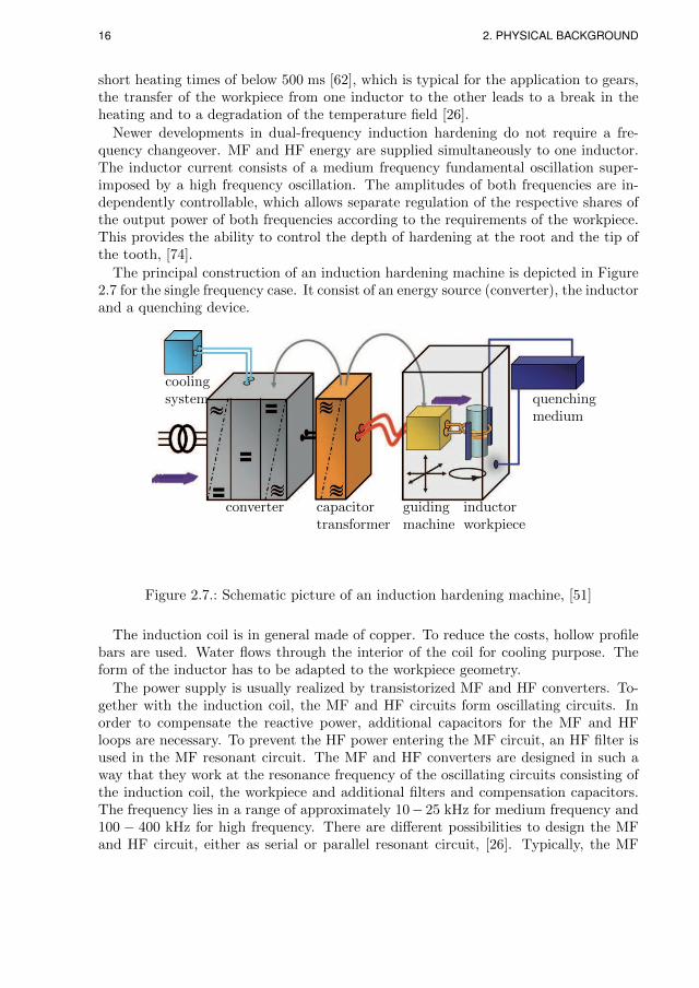
The principal construction of an induction hardening machine is depicted in Figure2.7 for the single frequency case. It consist of an energy source (converter), the inductorand a quenching device.
coolingsystem quenching
medium
converter capacitortransformer
guidingmachine
inductorworkpiece
Figure 2.7.: Schematic picture of an induction hardening machine, [51]
The induction coil is in general made of copper. To reduce the costs, hollow profilebars are used. Water flows through the interior of the coil for cooling purpose. Theform of the inductor has to be adapted to the workpiece geometry.
The power supply is usually realized by transistorized MF and HF converters. To-gether with the induction coil, the MF and HF circuits form oscillating circuits. Inorder to compensate the reactive power, additional capacitors for the MF and HFloops are necessary. To prevent the HF power entering the MF circuit, an HF filter isused in the MF resonant circuit. The MF and HF converters are designed in such away that they work at the resonance frequency of the oscillating circuits consisting ofthe induction coil, the workpiece and additional filters and compensation capacitors.The frequency lies in a range of approximately 10− 25 kHz for medium frequency and100 − 400 kHz for high frequency. There are different possibilities to design the MFand HF circuit, either as serial or parallel resonant circuit, [26]. Typically, the MF

2.2. The concept of multifrequency induction hardening 17
and HF circuit are connected to the induction coil by an inductive coupling, i. e. by atransformer.
The energy of the medium- and high-frequency converter can be regulated variable,typically the power is adjusted as relative value between 1 and 99 %. From a technicalpoint, the regulation of the energy is done by a pulse-width modulation for the mediumfrequency converter and by pulse package control for high frequency, see also [28, 85]for examples of the time-dependent current and voltage at the output of the MF andHF converter.
The inductor voltage or the current, which is required in 3D simulations of theinduction hardening process as input parameter, can be determined by a simulationof the resonant circuits. The oscillating circuits for each frequency can be representedby an equivalent circuit diagram that consists of capacitors, inductances and resistors,which are unknown and have to be determined by a parameter identification. Theinductor itself can be represented by an inductance and a resistance that are thecommon parts of each of the both resonant circuits. The parameters of the equivalentcircuit of the inductor are temperature dependent and have to be determined from the3D simulation, [26, 27].
In order to solve for the inductor current, a system of ordinary differential equationshas to be solved. The resulting current in the inductor will be periodic, but not neces-sarily harmonic. This is one of the reasons why the computation of the electromagneticfields is considered in the time domain instead of the typically used frequency domain.A further reason will be the nonlinear behaviour of material parameters such as themagnetic permeability. Due to the high complexity of the MF- and HF-converter, thesimulation of the converter by an equivalent circuit is not considered in this work.The input parameters for the simulation are taken from accessible quantities at themachine, e. g. measurements of the inverter current and knowledge of the transmissionratio.
In induction heating, the heat is generated directly in the workpiece and affects onlythe desired regions, which makes the process very energy efficient. Furthermore, due tothe short heating times, mechanical distortion is reduced and it is possible to integrateinduction hardening machines directly into the process chain. With the concept ofmultifrequency induction hardening a contour hardening of gears is possible, such thatfor industrial applications induction hardening has become a cost- and energy efficientalternative to classic case hardening by carburization, [8, 74].


Chapter 3.
The model
Introduction
In order to simulate induction heating processes we need to determine the distributionof the temperature θ and the high temperature phase austenite z in the workpiece.It is assumed that during the quenching process that follows the inductive heating,austenite transforms completely into martensite and is therefore an indicator of thehardening profile. The austenitization behaviour is directly linked to the temperaturedistribution by the transformation kinetics.
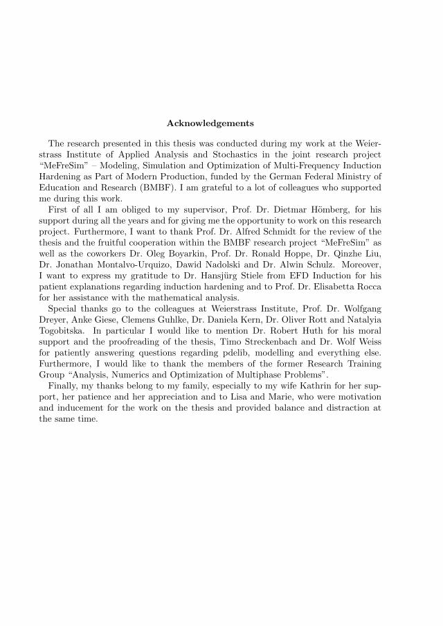
The heat is generated by the Joule effect: An alternating current flows through theinductor, which generates a temporal changing magnetic field. This magnetic fieldinduces a voltage and consequently generates eddy currents in the workpiece. Dueto resistive losses, heat is generated directly in the workpiece. The interdependencebetween the afore mentioned physical quantities is depicted in Figure 3.1.
Figure 3.1.: Schematic representation of the model
The physical effects during the induction heating process can be described by acoupled system of partial and ordinary differential equations. It comprises of theheat equation describing the temperature distribution, an ordinary differential equa-
19

20 3. THE MODEL
tion (ODE) to simulate the phase evolution and Maxwell’s equations to describe theelectromagnetic processes. This system is derived in the following.
For the geometric setting, we consider a domain D ⊂ R3 that consists of the inductorΩ, the workpiece Σ, and the surrounding air, see Figure 3.2. The connection to the
Σ
D
Ω
Figure 3.2.: Domain D consisting of the inductor Ω, the workpiece Σ and the sur-rounding air
converter is modelled by an idealized interface condition on a cross section of theinductor, cf. Section 3.1.4. The derivation of the partial differential equations requiresintegral identities that are given in Appendix A.1. Having introduced the geometricsetting, we start with the explanation of Maxwell’s equations.
3.1. Electromagnetic effects
3.1.1. Maxwell’s equations in differential form
The electromagnetic effects are described by Maxwell’s equations, which are presentedin their differential form [50]. They consist of a system of partial differential equationsconnecting the magnetic fieldH [A/m], the magnetic inductionB [Vs/m2], the electricfield E [V/m] and the electric displacement field D [As/m2]
curlE = −∂B∂t
divB = 0
curlH = J +∂D
∂tdivD = ρ.
(3.1)
The quantities on the right hand side are the current density J [A/m2] and the chargedensity ρ [As/m3]. The first equation is also denoted as Faradays law of induction.

3.1. Electromagnetic effects 21
It states that a time varying magnetic field is accompanied by an electric field. Theequation divB = 0 states that there are no magnetic sources, the magnetic fluxdensity B is a solenoidal field. Ampere’s law, the third equation in (3.1), describesthe fact that moving electric charges or electric currents generate a magnetic field.Finally, Gauss’ law relates the distribution of electric charges to the resulting electricdisplacement field.
Maxwell’s equations are completed by constitutive laws
D = εE and B = µH (3.2)
with material dependent parameters ε and µ, the electrical permittivity and the mag-netic permeability. The current density and the electric field are related by Fourier’slaw
J = σE, (3.3)
where σ denotes the electrical conductivity.The conservation of charge demands that the following compatibility condition holds.
Taking the divergence of the third equation in (3.1) together with div curlH = 0 yields
divJ +∂ρ
∂t= 0. (3.4)
Since the total charge is conserved, a change of the charge in a volume must be balancedby a flow of charge, i. e. an electric current, through the surface of the volume, [42].
3.1.2. Interface- and boundary conditions
For the electromagnetic fields, there hold certain continuity conditions at interfaces,where material properties change. These can be derived from Maxwell’s equations(3.1) with the help of Gauss’ and Stokes’ theorems, Thm. 3 and 4 in Appendix A.1.We denote by V an arbitrary volume element in space and by A an arbitrary surfaceelement. Then there holds∫
V
divB dx =
∫∂V
B ·nda and
∫A
curlE ·nda =
∫∂A
E · τ ds,
where n is the outward normal vector of the surface ∂V respectively A and τ denotesthe tangential vector of the line element ∂A.
We consider a volume element V = V1 ∪ V2 that is separated by an interface Γ =V1∩V2. Integration of divB = 0 over V and Vi, i = 1, 2, together with Gauss’ theorem(Thm. 3) yields
0 =
∫∂V
B ·nda−∫∂V1
B1 ·nda−∫∂V2
B2 ·nda
=
∫Γ
B1 ·nΓ da−∫Γ
B2 ·nΓ da = −∫Γ
JB ·nΓK da,
22 3. THE MODEL
where nΓ denotes the unit normal vector of the interface Γ, pointing from V2 into V1,Bi = B|Vi , i = 1, 2, and JBK = B2 −B1 denotes the jump of the magnetic inductionacross the interface Γ. Since the volume element V can be chosen arbitrary, thereholds
JB ·nΓK = 0, (3.5)
i. e. the normal component of the magnetic induction is continuous at interfaces.Now, we consider a surface A that intersects the interface Γ in a line L. Applying
Stokes’ theorem (Thm. 4), we finally derive by similar arguments the relation
JE × nΓK = 0, (3.6)
i. e. the tangential components of the electric field E are continuous. By analogousconsiderations, one obtains the relations
JH × nΓK = JΓ and JD ·nΓK = ρΓ (3.7)
with a surface current density JΓ and a surface charge density ρΓ, see e. g. [42].From these relations and the material laws (3.2) one obtains that the normal or
the tangential components of the electromagnetic fields exhibit discontinuities acrossmaterial interfaces. For simplicity, it is assumed that JΓ = 0 and ρΓ = 0. Then in thecase of jumping parameters µ and ε across the interface Γ there holds
JB × nΓK 6= 0, JH ·nΓK 6= 0, JE ·nΓK 6= 0 and JD × nΓK 6= 0. (3.8)
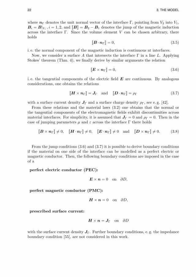
From the jump conditions (3.6) and (3.7) it is possible to derive boundary conditionsif the material on one side of the interface can be modelled as a perfect electric ormagnetic conductor. Then, the following boundary conditions are imposed in the caseof a
perfect electric conductor (PEC):
E × n = 0 on ∂D,
perfect magnetic conductor (PMC):
H × n = 0 on ∂D,
prescribed surface current:
H × n = JΓ on ∂D
with the surface current density JΓ. Further boundary conditions, e. g. the impedanceboundary condition [55], are not considered in this work.

3.1. Electromagnetic effects 23
3.1.3. Magnetic vector- and electric scalar potential
To reduce the system consisting of four partial differential equations plus materiallaws, the vector potential formulation of Maxwell’s equations is usually derived usingthe relations curl∇f = 0 and div curlv = 0, where f : D → R denotes a scalar valuedand v : D → R3 a vector valued function over D. From the relation divB = 0, cf.equation (3.1)2, we have the existence of the magnetic vector potential A such that
B = curlA.
Using (3.1)1, there holds
curl
(E +
∂A
∂t
)= 0.
As a consequence, we have the existence of the electric scalar potential φ such that
E = −∇φ− ∂A
∂t.
The magnetic vector potential A is not unique. The addition of an arbitrary gradientfield ∇ψ yields the same magnetic induction B. Therefore, certain gauging condi-tions need to be defined to ensure uniqueness. For induction phenomena, usually theCoulomb-gauging is used:
divA = 0. (3.9)
A typical assumption for the modelling of induction phenomena is that the term∂D/∂t is small compared to the current density J and can be neglected. Therefore,there is a coupling between the magnetic and the electric field only in conductiveregions, the dielectric displacement has no influence on the description of eddy currenteffects. The electric field and the current density are linked by Fourier’s law J = σE,cf. (3.3). Therefore, the total current density is given by
J = −σ∂A∂t− σ∇φ in D (3.10)
with σ = 0 in nonconducting regions D\(Σ ∪ Ω). Introducing this relation into (3.1)together with the compatibility condition divJ = 0, equation (3.4), and the gaugingcondition (3.9) yields the vector potential formulation of Maxwell’s equations
σ∂A
∂t+ curl
1
µcurlA+ σ∇φ = 0 on D
−div σ∇φ = 0 on Ω.
(3.11)
Please note that the inductor Ω is the only region with a prescribed source current orsource voltage. Therefore, the electric scalar potential vanishes everywhere except forthe domain Ω.
If we transform the boundary conditions introduced above to the vector potentialA, there holds
A× n = 0 (PEC), µ−1 curlA× n = 0 (PMC). (3.12)

24 3. THE MODEL
These conditions can be considered as analogue to standard Dirichlet- and Neumann-boundary conditions, respectively. At material interfaces there holds in analogy to(3.6)
JA× nK = 0, (3.13)
i. e. the tangential components of the magnetic vector potential A are continuous.In general, Maxwell’s equations are defined on an infinite domain. Since the mag-
netic field decreases to zero with exponential decay in the absence of electric currents,we set the magnetic vector potential A to zero if we are sufficiently away from theregion of interest, i. e. the workpiece and the inductor. Therefore, the surrounding airhas to be considered and we impose the boundary condition
A× n = 0 on ∂D. (3.14)
The electric scalar potential is only different from zero in the inductor Ω. Theinductor itself is represented by a torus. The connection clamps are ignored, they aremodelled by an interface condition on a cross section area of the inductor denoted asΓ. The normal derivative σ∇φ ·n represents the current. Since there is no currentflowing perpendicular to the surface of the inductor the following boundary conditionis imposed for the electric scalar potential
σ∇φ ·n = 0 on ∂Ω. (3.15)
A prescribed current or voltage source is realized by an interface condition on Γ. Theelectric current through the cross section Γ is always continuous. The voltage is definedas a potential difference between the connection pins. In our model this is realized bya jump condition for the potential φ, i. e.
Jσ∇φK ·n = 0 and JφK = u(t) on Γ, (3.16)
where J · K denotes the jump of a quantity across Γ and u(t) denotes the voltage. Thecharacterization of the scalar potential given above is due to [55].
3.1.4. Characterization of electric sources
In order to characterize the electric sources in terms of a given voltage or an electriccurrent in the inductor we introduce the source current density as
Jsrc = −σ∇φ, (3.17)
which has to satisfy divJsrc = 0. Then, for the total current density (3.10) there holds
J = −σ∂tA+ Jsrc. (3.18)
In the case of a rotational symmetric inductor Ω as e. g. in Figure 3.2 it is possibleto obtain an analytic expression for the electric scalar potential φ. In order to do this,we solve equation (3.11)2 with respect to cylindrical coordinates (r, ϕ, z) and assume

3.1. Electromagnetic effects 25
that the current in r- and z-direction is equal to zero. The equation −div σ∇φ = 0simplifies to
− 1
r2
∂
∂ϕ
(σ∂φ
∂ϕ
)= 0 on Ω.
As a solution we obtain
φ = C1ϕ and ∇φ =C1
reϕ, (3.19)
where the constant C1 is chosen to satisfy the boundary condition (3.16), i. e. C1 =u(t)/2π. The prescribed voltage in the inductor is denoted by a time dependentfunction u(t). If for example the voltage is harmonic with a fixed single frequencyf , then u(t) = umax cos(2πft). Transforming the solution (3.19) back to cartesiancoordinates, the following expression for the source current density Jsrc = −σ∇φ isobtained
Jsrc(x, t) = σu(t)
2πJ0(x) (3.20)
with a geometric form function
J0(x) = −
−y
x2+y2
xx2+y2
0
on Ω (3.21)
and equal to zero on D\Ω.In technical applications, usually the current is controlled. Therefore, also the case
of a prescribed inductor current i(t) is considered. The current through a cross sectionΓ of any conductor is determined as the integral of the current density in normaldirection, i. e.
i(t) =
∫Γ
J ·nda =
∫Γ
σ∇φ ·nda. (3.22)
With this condition it is possible to determine the current density J = −σ∇φ in theinductor from the solution of (3.19) also in the case of a given inductor current (thatcombines the impressed and the self-induced current). For this we assume that theinductor has a rectangular cross section with inner radius ri, outer radius ra and heighth. Then by equations (3.19) and (3.22) there holds
J(x, t) = i(t)log(ri/ra)
hJ0(x) in Ω (3.23)
with J0(x) given by (3.21).As we have seen from the considerations above, in both cases, voltage or current
control, the source current density can be written in the form
Jsrc(x, t) = j(t)J0(x) (3.24)
with a time dependent function j(t).

26 3. THE MODEL
In the case of multifrequency induction hardening with a prescribed inductor current,the current density J consists of the superimposed medium and high frequency partsof the source current. Assume for simplicity a harmonic source current, then
J(x, t) = (pmf(t)Imf cos(2πfmft) + phf(t)Ihf cos(2πfhft))log(ri/ra)
hJ0(x) (3.25)
in the inductor, where Imf/hf denote the maximum amplitudes of the MF and HFcurrent. By pmf/hf(t) ∈ [0, 1] we denote a relative fraction of the medium and highfrequency current, that corresponds to the relative power that is used as a controlparameter for the induction hardening machine. In general, the inductor current isperiodic but not necessarily harmonic. We account for this fact by considering thevector potential equation in the time domain instead of the usually used harmonicapproach that is limited to harmonic excitations.
3.2. Phase fraction of austenite
During the heating process only the formation of the high temperature phase austeniteis of interest. The volume fraction of austentite is given by the variable z(x, t) withz ∈ [0, 1]. The initial microstructure is in general not known. It might be a phasemixture consisting of ferrite, martensite, pearlite or bainite. Its volume fraction isdenoted by z0(x, t). The initial state and austenite always sum up to one such thatz0 = 1− z. It is assumed that the transformation kinetics can be described by a ratelaw in the form of a Leblond-Devaux-law [49], which we use in the following generalizedform [38],
∂tz(t) =zr(θ)
τ(θ)[zeq(θ)− z]+
z(0) = 0.
(3.26)
With [ · ]+ the positive part of a function is denoted. The parameters r(θ), zeq(θ) andτ(θ) denote material dependent functions, that have to be determined from experi-mental measurements or fits to TTT/TTA diagrams like Figure 2.3 and 2.4. In orderto reduce the complexity, the temperature dependence of r might be ignored. The ratelaw (3.26) does not depend explicitly on the space coordinate x. The spatial depen-dence of the phase fraction of austenite is only introduced by the spatial dependenceof the temperature θ.
In the case of induction hardening, one has to deal with very short heating timesand consequently, very high heating rates. Referring to literature, measurements forshort time austenitization were performed by Miokovic, [54]. Their approach to modelthe phase transformation behaviour is based on a generalized Johnson-Mehl-Avramiequation [2, 44], which is given in the form
∂tz(t) = nC exp
(−∆H
k θ
)ln
(1
1− z
)n−1n
(1− z).
The constant k = 8.617 · 10−5 eV/K denotes the Boltzmann constant. Further pa-rameters were determined as n = 1.525, C = 2.84 · 1020 s−1 and ∆H = 4.185 eV.

3.3. Balance of energy 27
Introducing a linearization of the logarithm, i. e. − ln(1 − z) ≈ z, the rate law abovefits into the general form of equation (3.26).
3.3. Balance of energy
In order to determine the temperature distribution in the workpiece Σ we considerthe balance of energy. The temperature distribution in the surrounding air and inthe induction coil is not considered. In practical applications, the inductor is cooled.Simulating the cooling process is a complicated task and out of scope of this thesis.
The balance of internal energy is given by the following equation
ρ∂e
∂t+ div q = Q in Σ, (3.27)
where ρ denotes the constant density1 , e the specific internal energy of the system, qthe heat flux and Q the heat source, which results as the Joule heat
Q = J ·E = σ |∂tA|2 .
In order to ensure thermodynamic consistency of the model, we assume that theSecond Law of Thermodynamics (2nd law) is satisfied. It states the existence of a pairof quantities, the specific entropy s and the entropy flux ϕ, that are connected by abalance equation
ρ∂s
∂t+ divϕ = ζ,
where ζ denotes the entropy production [56]. The statement of the 2nd law is thatthe entropy production is nonnegative for every thermodynamic process, i. e. for everysolution of the underlying partial differential equations,
ζ ≥ 0.
In order to evaluate the 2nd law, we introduce the Helmholtz free energy as thermo-dynamic potential
ψ = e− θs.
The temperature θ and the volume fraction of austenite z are the unknown fields ofinterest. It is assumed that the free energy depends on these quantities such that thereexists a representation ψ = ψ(θ, z). The time derivative of ψ is given by
∂tψ = ∂te− s∂tθ − θ∂ts and ∂tψ =∂ψ
∂θ∂tθ +
∂ψ
∂z∂tz. (3.28)
Introducing the entropy balance into (3.28)1 yields
θζ = ρ∂te− ρ∂tψ − ρs∂tθ + θ divϕ.
1The workpiece Σ is modelled as an incompressible rigid body, mechanical displacements and stressesresulting form thermal expansion, transformation induced plasticity or external forces are ignored.Therefore, the density is constant.

28 3. THE MODEL
With the balance of internal energy and (3.28)2 we obtain the following expression forthe entropy inequality
θζ = σ |∂tA|2 −q
θ∇θ − ρ∂ψ
∂θ∂tθ − ρ
∂ψ
∂z∂tz − ρs∂tθ − θ div
q
θ+ θ divϕ ≥ 0. (3.29)
For simple, incompressible bodies, the entropy flux is given as
ϕ =q
θ.
Then, the last two terms drop out of expression (3.29). The remaining inequality has tohold for every thermodynamic process, i. e. for all solutions of the underlying partialdifferential equations. Assume we have a solution with homogeneous temperature,constant phase fraction z and vanishing magnetic potential but arbitrary ∂tθ. Then inorder to not violate inequality (3.29), there has to hold the following relation, whichis standard in literature,
s = −∂ψ∂θ. (3.30)
With this relation, inequality (3.29) has the form
θζ = σ |∂tA|2 −q
θ∇θ − ρ∂ψ
∂z∂tz ≥ 0.
The Joule heat is a nonnegative quantity. The remaining terms have a product struc-ture. In order to not violate the entropy inequality, we assume that the heat flux isgiven by Fourier’s law
q = −κ∇θ (3.31)
with κ > 0 denoting the positive heat conductivity. Furthermore, we assume thatthere exists a quantity Ξ > 0 such that
∂tz = −Ξ∂ψ
∂z. (3.32)
With the definition of the specific heat at constant volume, cV = θ∂s/∂θ, and thedefinition of the latent heat, L = ∂e/∂z, we compute for the time derivative of theinternal energy
∂te = cV ∂tθ + L∂tz.
The balance of internal energy becomes finally
ρcV ∂tθ − div κ∇θ = σ |∂tA|2 − ρL ∂tz in Σ and t ∈ (0, T ). (3.33)
Remark 3.1. In the energy balance above, the specific heat at constant volume, cV ,appears. From a practical point of view, this quantity is hard to measure. Experimentsare usually carried out at constant pressure, such that the specific heat at constantpressure, cp, is an accessible quantity. The specific heat capacity denotes the energythat is necessary to heat up a material by 1 K. In the case of constant pressure,

3.4. Characterization of the material parameters 29
energy is also required for the volumetric change of the body due to thermal expansion.Therefore, there holds cp > cV . For solid materials, the difference cp− cV is small. Inaddition, we model the workpiece as incompressible body and ignore deformations dueto thermal expansion and volumetric changes due to the phase transition. In this caseit is assumed that cV = cp.
Remark 3.2. With e = ψ − θs and (3.30) the latent heat can be related directly tothe free energy ψ by
L(θ, z) =∂e
∂z=∂ψ
∂z− θ ∂s
∂z=∂ψ
∂z− θ ∂
2ψ
∂θ∂z. (3.34)
Using relation (3.32) it is possible to get an explicit formulation for the latent heat,that is related to the evolution equation for the volume fraction z. The positive quantityΞ can be used to adapt the in general nonlinear expression for the latent heat
L(θ, z) =∂ψ
∂z− θ ∂
2ψ
∂θ∂z= −Ξ−1 z
r
τ[zeq − z]+ + Ξ−1 ∂
∂θ
(zr
τ[zeq − z]+
)to thermodynamic measurements.
Next, we consider the boundary conditions for the temperature. In general, at theboundary of the workpiece ∂Σ there occur heat losses due to radiation and convection.This can be described by the following general boundary condition
−κ∇θ ·n = α(θ4 − θ40) + η(θ − θ0) on ∂Σ.
Here, α denotes the radiation coefficient, η the heat transfer coefficient and θ0 theambient temperature. To be precise, α is the product of the Stefan Boltzmann constantσ = 5.6710−8 W/m2K4 and the material emissivity coefficient ε ∈ [0, 1].
If we compare the energy of the heat radiation to the heat energy that is generatedin the workpiece due to the eddy currents, we observe that the radiation energy is bymagnitudes smaller. Typically, in applications of induction hardening the necessarysurface energy density lies in the range of about 0.5 − 15 kW/cm2. Estimating thelosses due to radiation with a surface temperature of θ = 1073 K and ε = 1, which is anoverestimation, since the surface is not black, gives an approximate loss of 7.5 W/cm2.Consequently, it is justified to neglect losses due to radiation. Finally, we assume aRobin type boundary condition for the temperature at the surface of the workpiece∂Σ in the following form
κ∇θ ·n+ ηθ = g on ∂Σ, (3.35)
where g = ηθ0 denotes a given function.
3.4. Characterization of the material parameters
In general, the material parameters are temperature dependent and they are differentfor each material and also for each phase. Therefore, they depend on the space x, the
30 3. THE MODEL
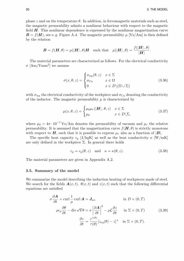
phase z and on the temperature θ. In addition, in ferromagnetic materials such as steel,the magnetic permeability admits a nonlinear behaviour with respect to the magneticfield H. This nonlinear dependence is expressed by the nonlinear magnetization curveB = f(H), see e. g. Figure A.4. The magnetic permeability µ [Vs/Am] is then definedby the relation
B = f(H, θ) = µ(|H| , θ)H such that µ(|H| , θ) =f(|H| , θ)|H|
.
The material parameters are characterized as follows. For the electrical conductivityσ [Am/Vmm2] we assume
σ(x, θ, z) =
σwp(θ, z) x ∈ Σ
σCu x ∈ Ω
0 x ∈ D\(Ω ∪ Σ)
(3.36)
with σwp the electrical conductivity of the workpiece and σCu denoting the conductivityof the inductor. The magnetic permeability µ is characterized by
µ(x, θ, z) =
µ0µr(|H| , θ, z) x ∈ Σ
µ0 x ∈ D\Σ,(3.37)
where µ0 = 4π · 10−7 Vs/Am denotes the permeability of vacuum and µr the relativepermeability. It is assumed that the magnetization curve f(H, θ) is strictly monotonewith respect to H, such that it is possible to express µr also as a function of |B|.
The specific heat capacity cp [J/kgK] as well as the heat conductivity κ [W/mK]are only defined in the workpiece Σ. In general there holds
cp = cp(θ, z) and κ = κ(θ, z). (3.38)
The material parameters are given in Appendix A.2.
3.5. Summary of the model
We summarize the model describing the induction heating of workpieces made of steel.We search for the fields A(x, t), θ(x, t) and z(x, t) such that the following differentialequations are satisfied
σ∂A
∂t+ curl
1
µcurlA = Jsrc in D × (0, T )
ρcp∂θ
∂t− div κ∇θ = σ
∣∣∣∣∂A∂t∣∣∣∣2 − ρL∂z∂t in Σ× (0, T )
∂z
∂t=zr(θ)
τ(θ)[zeq(θ)− z]+ in Σ× (0, T ).
(3.39)

3.5. Summary of the model 31
As boundary conditions, we impose
A× n = 0 on ∂D
κ∇θ ·n+ ηθ = g on ∂Σ.(3.40)
The model is completed by initial conditions
A(x, 0) = A0(x) in D
θ(x, 0) = θ0(x) in Σ
z(0) = 0 in Σ.
(3.41)
In the next chapter, analytical investigations to show existence and uniqueness ofa simplified model are carried out. In contrast to (3.39–3.41) it is assumed that thematerial parameters depend only on the space x and the phase z, but not on thetemperature θ. The numerical simulation algorithm for the full model (3.39–3.41)together with various examples of induction hardening of discs and gears is presentedin Chapters 5 and 6.


Chapter 4.
Analysis of a simplified model
Introduction
In this chapter, the analysis of a simplified model is considered. We show well-posedness of the problem and derive regularity results for solutions of a weak for-mulation of system (3.39) with modified material parameters. For simplicity it willbe assumed that all material parameters are independent of the temperature θ suchthat they only depend on the space x and the phase fraction of austenite z. Further-more, the nonlinearity in the magnetic permeability µ is ignored. Within this chapter,partial derivatives will be denoted by a subscript index to simplify the notation, e. g.∂A/∂t = At. The main part of this chapter has been published in [39].
4.1. Notation and preliminary assumptions
We consider the geometric setting as introduced in Chapter 3, cf. Figure 3.2, withD ⊂ R3 denoting the hold all domain containing the inductor coil Ω and the workpieceΣ. It is assumed that Ω ⊂ D, Σ ⊂ D, Ω∩Σ = ∅ and ∂Ω, ∂Σ, ∂D are of class C1,1. WecallG = Ω∪Σ the set of conductors and define the space-time domain asQ = Σ×(0, T ).
The simplified material parameters are characterized as follows. It is assumed thatthe electrical conductivity σ and the magnetic permeability µ are sufficiently regularand bounded from below and above. They may depend both on the spatial variablesand also on the phase parameter z but not on the temperature θ as in the generalsetting:
σ(x, z) =
σwp(z), x ∈ Σ ,
σCu, x ∈ Ω ,
0, x ∈ D \G ,(4.1)
with its derivative with respect to the z-variable
σz(x, z) =
σ′wp(z), x ∈ Σ ,
0, x ∈ D \ Σ ,(4.2)
and
µ(x, z) =
µwp(z), x ∈ Σ ,
µ0, x ∈ D \ Σ .(4.3)
33

34 4. ANALYSIS OF A SIMPLIFIED MODEL
with
µz(x, z) =
µ′wp(z), x ∈ Σ ,
0, x ∈ D \ Σ .(4.4)
The specific heat and the heat conductivity are assumed to be constant. For simplicity,we take r = 0 in the rate law describing the evolution of the phase fraction.
In the following sections we will study the well-posedness for the Cauchy systemassociated to a suitable variational formulation of the simplified model to describethe induction heating process. For completeness, we repeat the system of partialdifferential equations of the reduced problem
σAt + curlµ−1 curlA = Jsrc in D × (0, T )
ρcpθt − div κ∇θ = σ |At|2 − ρLzt in Σ× (0, T )
zt =1
τ(θ)[zeq(θ)− z]+ in Σ× (0, T )
(4.5)
supplemented with boundary and initial conditions
A× n = 0 on ∂D
κ∇θ ·n+ ηθ = g on ∂Σ
A(x, 0) = A0(x) in D
θ(x, 0) = θ0(x) in Σ
z(0) = 0 in Σ.
(4.6)
In order to derive the weak formulation of the Cauchy problem, we recall the defi-nitions of the generalized curl and div operators. For this, we introduce the followingnotation. Let us denote with the symbol W the vector-valued counterpart of the Ba-nach space W . We use the symbol Lq(U×(0, t)) for the space Lq(0, t;Lq(U)), for everyq ∈ [1,+∞), t ∈ (0, T ] and U ⊂ R3 a bounded domain of class C1,1. Let p ∈ (1,+∞)and ψ ∈ Lp(D), then, we write curlψ ∈ Lp(D) if there exists ξ ∈ Lp(D) such that∫
D
ψ curlφdx =
∫D
ξφdx for all φ ∈ C∞c (D).
We define curlψ := ξ as the uniquely determined vector ξ. Analogously, we writedivψ ∈ Lp(D) if there exists ζ ∈ Lp(D) such that∫
D
ψ · ∇ηdx = −∫D
ζηdx for all η ∈ C∞c (D).
We define divψ := ζ as the uniquely determined element ζ. Then, we introduce theBanach spaces (with the graph norms)
Lpcurl(D) = ψ ∈ Lp(D) : curlψ ∈ Lp(D)

4.1. Notation and preliminary assumptions 35
and
Lpdiv(D) = ψ ∈ Lp(D) : divψ ∈ Lp(D).
For ψ ∈ L2curl(D) we define the linear bounded trace operator γτ (ψ) using the well-
known Green’s formula (cf. e. g. [25])∫D
ψ · curlφdx−∫D
curlψ ·φdx = −∫∂D
(n×ψ) ·φds =: 〈γτ (ψ),φ〉 , (4.7)
for all φ ∈ H1(D), where (with an abuse of notation) the integral over ∂D has tobe understood as the duality between H−1/2(∂D) and H1/2(∂D) and n denotes theoutward unit normal vector to ∂D. Similarly, for ψ ∈ L2
div(D) we introduce the linearbounded trace operator γn(ψ) by the Green’s formula∫
D
ψ · ∇φdx+
∫D
divψ φdx =
∫∂D
(n ·ψ)φds =: 〈γn(ψ), φ〉 , (4.8)
for all φ ∈ H1(D), where (with an abuse of notation) the integral over ∂D has to beunderstood as the duality between H−1/2(∂D) and H1/2(∂D). Finally, we introducethe Hilbert space
X = v ∈ L2curl(D) : div v = 0 and γτ (v) = 0 .
Notice that, since ∂D ∈ C1,1 the space X equipped with the norm
‖v‖X = ‖curlv‖L2(D)
is a closed subspace of H1(D). Moreover, let us notice that, from the Green’s formula itfollows that: if A ∈ X, then γn(A) = 0. Indeed, if we denote by w = curlA ∈ L2(D),then divw = 0 and γn(w) ∈ H−1/2(∂D). Moreover the following Green’s formulashold true for every test function φ ∈ H1(D):
〈γn(w), φ〉 =
∫D
(divw φ+w · ∇φ) dx =
∫D
curlA · ∇φdx
=
∫D
curlA · ∇φ−A · curl∇φdx
=〈γτ (A),∇φ〉 .
(4.9)
Hence, if A ∈ X, then γn(curlA) = 0 (cf. e. g. [30, Chapter 2]).
The following results are necessary to obtain the regularity results. The first one isan embedding result that is a consequence of [32, Thm. 3.3]. The complete proof of amore general result can be found in [22, Prop. 2.2].

36 4. ANALYSIS OF A SIMPLIFIED MODEL
Lemma 4.1. Let U ⊂ R3 be a bounded C1 domain, then the space
Wp,α(U) = u ∈ Lpcurl(U) ∩ Lpdiv(U) : γn(u) ∈ Lα(∂U)
continuously embeds in the space Lξ(U) for ξ := min 3α2 , p
∗, where p∗ is the Sobolevembedding exponent
p∗ :=
3p
3−p if 1 ≤ p < 3 ,
s ∈ [1,+∞) if p = 3 ,
+∞ if p > 3 .
Moreover, we recall the following interpolation inequality, holding true for p, q, r ∈[1,+∞], with p < r < q, 1/r = α/p+ (1− α)/q, α ∈ (0, 1), and v ∈ Lq(D):
‖v‖Lr(D) ≤ ‖v‖αLp(D)‖v‖1−αLq(D) . (4.10)
Now, we precisely state the assumptions on the data.
4.2. Hypotheses
We list here our basic assumptions on the functions σ, µ, J0, j, τ , and zeq in (4.5),where we take the constants cp, κ and η equal to 1, for simplicity.
Hypothesis (H). Assume that
(i) σ(x, z) : D × [0, 1] → R is a piecewise continuous and Lipschitz continuous(w.r.t. z for almost all x ∈ D) function defined in (4.1) and (4.2), where σwp ∈C1,1([0, 1]), σCu ∈ R+. Assume moreover that there exist two constants 0 < σ ≤σ such that
σ ≤ σ(x, z) ≤ σ in D × [0, 1] ;
(ii) µ(x, z) : D×[0, 1]→ R is a piecewise continuous and Lipschitz continuous (w.r.t.z for almost all x ∈ D) function defined in (4.3), (4.4), where µwp ∈ C1,1([0, 1]),µ0 ∈ R+. Assume moreover that there exist two constants 0 < µ ≤ µ such that
µ ≤ µ(x, z) ≤ µ in D × [0, 1] ;
(iii) j ∈ H1(0, T ), J0 : D → R3 is an L2curl(D)-function defined in (3.21);
(iv) τ, zeq ∈ C2(R), L ∈ C0,1(R× [0, 1]) and there exist positive constants 0 < τ∗ ≤τ∗, M > 0 and CL > 0 such that
τ∗ ≤ τ(θ) ≤ τ∗, 0 ≤ zeq(θ) ≤ 1 for all θ ∈ R, ‖τ‖C2(R) ≤M, ‖zeq‖C2(R) ≤M ,
and |L(θ, z)| ≤ CL for all (θ, z) ∈ R× [0, 1] ;
(v) g ∈ L∞(0, T ;L∞(∂Σ));

4.3. Weak formulation and main theorem 37
(vi) A0 ∈ X ∩H3(D), θ0 ∈W 2,5/3(Σ).
With these preliminary assumptions we are now able to derive the weak formulationfor problem (4.5) and state the main result on the well-posedness and the stabilityestimates. The analytical results are presented in Section 4.3. The proofs are carriedout in Section 4.4.
4.3. Weak formulation and main theorem
We will now state the weak formulation of the Cauchy problem (4.5), (4.6), (3.24) and(3.34).
Problem (P). Find a triple (A, θ, z) with the regularity properties
A ∈ H2(0, T ;L2(D)) ∩W 1,∞(0, T ;X), curlA ∈ L∞(0, T ;L6(D)) , (4.11)
θ ∈W 1,5/3(0, T ;L5/3(Σ)) ∩ L5/3(0, T ;W 2,5/3(Σ)) ∩ L2(0, T ;H1(Σ)) ∩ L∞(Q) ,(4.12)
z ∈W 1,∞(0, T ;W 1,∞(Σ)), 0 ≤ z < 1 a.e. in Q , (4.13)
solving the following system∫G
σ(x, z)At ·vdx+
∫D
1
µ(x, z)curlA · curlvdx =
∫Ω
j(t)J0(x) ·vdx (4.14)
for all v ∈ X, a.e. in (0, T ) ,
θt −∆θ = −L(θ, z)zt + σ(x, z)|At|2 a.e. in Q , (4.15)
zt =1
τ(θ)[zeq(θ)− z]+ a.e. in Q , (4.16)
A× n = 0 a.e. on ∂D × (0, T ), ∇θ ·n+ θ = g a.e. on ∂Σ× (0, T ) , (4.17)
A(0) = A0 a.e. in D, θ(0) = θ0, z(0) = 0 a.e. in Σ (4.18)
and satisfying the following estimate
‖A‖H2(0,T ;L2(D))∩W 1,∞(0,T ;X) + ‖ curlA‖L∞(0,T ;L6(D))
+ ‖θ‖W 1,5/3(0,T ;L5/3(Σ))∩L5/3(0,T ;W 2,5/3(Σ))∩L2(0,T ;H1(Σ))∩L∞(Q)
+ ‖z‖W 1,∞(0,T ;W 1,∞ (Σ)) ≤ S ,(4.19)
where the constant S depends on the data of the problem.
The main result is stated in the following theorem.

38 4. ANALYSIS OF A SIMPLIFIED MODEL
Theorem 1. Let Hypothesis (H) hold true. Then, there exists a unique solution toProblem (P). Moreover, if we denote by (Ai, θi, zi), i = 1, 2, two triples of solutionscorresponding to data (A0,i, θ0,i, ji), then, there exists a positive constant C = C(S)(cf. estimate (4.19)) such that the following stability estimate holds true
‖(A1 −A2)(t)‖2L2(D) + ‖ curl(A1 −A2)‖2L2(D×(0,T ))
+ ‖∂t(A1 −A2)(t)‖2L2(D) + ‖ curl(∂t(A1 −A2))‖2L2(D×(0,T ))
+ ‖(θ1 − θ2)(t)‖2L2(Σ) + ‖θ1 − θ2‖2L2(0,T ;H1(Σ))
+ ‖(z1 − z2)(t)‖2H1(Σ) + ‖∂t(z1 − z2)‖2L2(0,T ;H1(Σ))
≤ C(‖A0,1 −A0,2‖2X + ‖(∂t(A1 −A2))(0)‖2L2(D) + ‖θ0,1 − θ0,2‖2L2(Σ)
+‖j1J0 − j2J0‖2L2(0,T ) + ‖j′1J0 − j′2J0‖2L2(0,T )
)for all t ∈ [0, T ] .
(4.20)
4.4. Proof of the existence result
In this section we prove Theorem 1 in three steps: first, we prove local existence ofsolutions by means of Schauder fixed point argument. Secondly, we prove the globala priori estimates necessary in order to extend the solution to the whole time interval[0, T ]. Finally, we prove the stability estimate (4.20) entailing, in particular, uniquenessof the solution to Problem (P).
4.4.1. Existence of a (local in time) solution
We start the proof by solving (locally in time) Problem (P) by means of a standardfixed point argument of Schauder type.
For a fixed T0 ∈ (0, T ] (which shall be specified later on) and a fixed constant R > 0,let us introduce the space
O = θ ∈ L2(0, T0;L2(Σ)) : ‖θ‖L2(0,T0;L2(Σ)) ≤ R .
In the following, we shall construct an operator T , which maps O onto itself for asuitable time 0 < T0 ≤ T , in such a way that any fixed point of T yields a solutionto Problem (P). We shall prove that T is compact and continuous w.r.t. the topologyof L2(0, T0;L2(Σ)). Hence, by the Schauder theorem T admits (at least) a fixed pointθ in O, whence the existence of a solution (A, θ, z) to the Cauchy Problem (P) onthe interval [0, T0]. Finally, the (local) uniqueness result will be a consequence of thestability estimate (4.44) below.
Definition of the fixed point map T . We construct the operator T in this way:given θ ∈ O, the operator
T : O→ L5/3(0, T ;W 2,5/3(Σ)) ∩W 1,5/3(0, T ;L5/3(Σ))
T : θ 7→ θ where θ solves

4.4. Proof of the existence result 39
θt −∆θ = −L(θ, z)zt + σ(x, z)|At|2 a.e. in Q , (4.21)
∇θ ·n+ θ = g a.e. on ∂Σ× (0, T ) , (4.22)
θ(0) = θ0, a.e. in Σ , (4.23)
and z ∈W 1,∞(0, T ;L∞(Σ)), A ∈ H1(0, T ;X) ∩W 1,∞(0, T ;L2(D)) solve
zt =1
τ(θ)
[zeq(θ)− z
]+a.e. in Q, z(0) = 0 a.e. in Σ , (4.24)∫
G
σ(x, z)At ·vdx+
∫D
1
µ(x, z)curlA · curlvdx =
∫Ω
j(t)J0(x) ·vdx (4.25)
for all v ∈ X, a.e. in (0, T ), A(0) = A0, a.e. in D .
T maps O in itself. Notice that, given θ ∈ O, [40, Lemma 2.5] ensures that thereexists a unique solution z ∈W 1,∞(0, T0;L∞(Σ)) to (4.24) such that
‖z‖W 1,∞(0,T0;L∞(Σ)) ≤ C1 ,
with C1 independent of θ, and 0 ≤ z < 1 a.e. in Σ.Then, given z ∈ W 1,∞(0, T0;L∞(Σ)), it is possible to find a unique solution A ∈
H1(0, T0;X) ∩W 1,∞(0, T0;L2(D)) to (4.25) by means of a standard implicit time dis-cretization scheme (cf. e. g. the monograph [45]). The basic estimates are the discreteversions of the ones which follow from taking v = At in (4.25) (cf. also the followingSecond estimate) and taking the time derivative of (4.25) with v = At (cf. also thefollowing and Third estimate). These give the bound
‖A‖H1(0,T0;X)∩W 1,∞(0,T0;L2(D)) ≤ C2 ,
with C2 independent of θ. Then, using the fact that At ∈ L∞(0, T0;L2(D)), At ∈L2(0, T0;X) → L2(0, T0;L6(D)) (due to the continuous embedding of H1(D) intoL6(D)) and employing the interpolation inequality (4.10) with q = 6, p = 2 andr = 10/3, we get At ∈ L10/3(D× (0, T0)). This implies that |At|2 ∈ L5/3(D× (0, T0))on the right hand side of (4.21) and
‖At‖L10/3(D×(0,T0)) ≤ C3 .
Applying now the standard maximal regularity results in Lp-spaces (cf. e. g. [64,Thm. 3.1, Prop. 3.3]) to (4.21–4.23), and Hyp. (H) (iv), we can conclude that thereexists a unique θ ∈ L5/3(0, T0;W 2,5/3(Σ))∩W 1,5/3(0, T0;L5/3(Σ)) solving (4.21–4.23)satisfying
‖θ‖L5/3(0,T0;W 2,5/3(Σ))∩W 1,5/3(0,T0;L5/3(Σ)) ≤ C4 ,
with C4 independent of θ. Moreover, testing equation (4.21) by θ, we get
‖θ‖L2(0,T0;H1(Σ))∩L∞(0,T0;L2(Σ)) ≤ C5 ,

40 4. ANALYSIS OF A SIMPLIFIED MODEL
with C5 independent of θ. This implies in particular
‖θ‖L2(0,t;L2(Σ)) ≤ t1/2‖θ‖L∞(0,T0;L2(Σ)) ≤ t1/2C5 for every t ∈ [0, T0) .
If we choose T0 such that T1/20 C5 ≤ R, then the map T maps O into itself.
T is compact. The map T is compact due to the compact embedding
L5/3(0, T0;W 2,5/3(Σ)) ∩ L2(0, T0;H1(Σ)) ∩W 1,5/3(0, T0;L5/3(Σ))
→→ L2(0, T0;L2(Σ)) (4.26)
(cf. [78, Thm. 4, Cor. 5]).
T is continuous. The continuity of T follows from these facts:
1. From [40, Lemma 2.5] we have that, if θk → θ strongly in L2(0, T0;L2(Σ)),for k → +∞, then zk → z strongly in W 1,p(0, T0;Lp(Σ)) for every p ∈ [1,+∞),where zk and z are the solutions to (4.24) corresponding to θk and θ, respectively.
2. From the compact embedding of H1(0, T0;X)∩W 1,∞(0, T0;L2(D)) into Lq(D×(0, T0)) (for q ∈ [1, 10/3)), we get that ∂tAk → ∂tA strongly in Lq(D × (0, T0))for every q ∈ [1, 10/3), and curlAk → curlA weakly in H1(0, T0;L2(D)) (at leastfor a subsequence of k), where Ak are the solutions to (4.25) corresponding to zk.There remains to show that the limit A is the solution of (4.25) correspondingto z. Then, the convergence will hold true for the whole sequence Ak. Indeed,from the strong convergence of zk and using Hyp. ((H)) (i), (ii), we get thatσ(x, zk) → σ(x, z) and µ(x, zk) → µ(x, z) strongly in Lp(0, T0;Lp(Σ)) for everyp ∈ [1,+∞). This implies that we can pass to the limit for k → +∞ and thelimit A solves (4.25).
3. Finally, we can come back to equation (4.21) and we have that |∂tAk|2 → |∂tA|2in Ls(Σ× (0, T0)) for some s ∈ [1, 5/3) because ∂tAk → ∂tA strongly in Lq(D×(0, T0)) for every q ∈ [1, 10/3) and ∂tAk, ∂tA are bounded (uniformly in k)in L2(D × (0, T0)). This fact, together with the strong convergence ∂tzk →∂tz strongly in Lp(0, T0;Lp(Σ)) for every p ∈ [1,+∞) and L(θk, zk) → L(θ, z)strongly in L2(0, T0;L2(Σ)) (cf. Hyp. (H) (iv)), imply that also θk → θ stronglyin L2(Σ× (0, T0)) for k → +∞, where θk (and θ) are are the solutions to (4.21)corresponding to zk, Ak (and z, A), respectively.
Hence, by the Schauder theorem T admits (at least) one fixed point θ in O, whencethe existence of a solution (A, θ, z) to (4.11)–(4.18) on the interval [0, T0] with
A ∈ H2(0, T ;L2(D)) ∩W 1,∞(0, T ;X), curlA ∈ L∞(0, T ;L6(D)) ,
θ ∈W 1,5/3(0, T ;L5/3(Σ)) ∩ L5/3(0, T ;W 2,5/3(Σ)) ∩ L2(0, T ;H1(Σ)) ∩ L∞(Q) ,
z ∈W 1,∞(0, T ;L∞(Σ)), 0 ≤ z < 1 a.e. in Q.

4.4. Proof of the existence result 41
4.4.2. Global a priori estimates
In order to extend the solution to the whole time interval [0, T ] we need to provesuitable global a priori estimates that are independent of T0. In what follows thepositive constants are denoted by the same symbol C even if they are different fromline to line. They may depend on σ, µ, τ , zeq, A0, θ0, g, j, J0, and T , but not on T0.
First estimate. First of all, we can apply [40, Lemma 2.5] to the equation (4.16)entailing the following estimate:
‖z‖W 1,∞(0,T0;L∞(Σ)) ≤ C , 0 ≤ z(x, t) < 1 a.e. in Q . (4.27)
Second estimate. Take t ∈ (0, T0) and v = At in (4.14). Using Hyp. (H) (i), (ii)(cf. also (4.4)), we get (using the symbol s for the time variable and x for the spacevariable inside the integrals, but making the dependence on x and s explicit only whenit is necessary):
σ
t∫0
∫G
|As|2 dxds+
t∫0
∫D
1
µ(x, z)curlA · curlAsdxds (4.28)
≤t∫
0
∫Ω
j(s)J0(x) ·Asdxds .
Now, integrating by parts in time the second term in (4.28), we get
t∫0
∫D
1
µ(x, z)curlA · curlAsdxds =
1
2
t∫0
∫Σ
µ′wp(z)zs
µ2(x, z)| curlA|2 dxds
+
∫D
1
2µ(x, z(t))| curlA|2(t)dx
− 1
2
∫D
1
µ(x, 0)| curlA0|2 dx .
Then, using estimate (4.27) and Hyp. (H) (ii), we get
σ
2
t∫0
∫G
|As|2 dxds+1
2µ
∫D
| curlA|2(t)dx ≤ 1
2µ
∫D
| curlA0|2 dx
+ C
t∫0
∫D
| curlA|2 dxds+
t∫0
∫Ω
|j(s)|2|J0|2 dxds
.

42 4. ANALYSIS OF A SIMPLIFIED MODEL
Using now a standard Gronwall lemma together with Hyp (H) (vi), we obtain
t∫0
∫G
|As|2 dxds+
∫D
| curlA|2(t)dx ≤ C
1 +
t∫0
∫Ω
|j(s)|2|J0(x)|2 dxds
. (4.29)
Third estimate. We can now formally (in order to make it rigorous one shouldperform the estimate e. g. on a time discrete scheme) differentiate (4.14) with respectto t and take v = At as test function. Integrating over (0, t), using Hyp (H) (i), (ii), aswell as the integration by parts in time in the second summand, gives (cf. also (4.2),(4.4)):
σ
2
∫G
|At|2(t)dx+1
2µ
t∫0
∫D
| curlAs|2 dxds ≤ σ∫D
|At(0)|2 dx
− 1
2
t∫0
∫Σ
σ′wp(z)zs |As|2 dxds+
t∫0
∫Σ
µ′wp(z)zs
µ2(x, z)curlA · curlAsdxds
+
t∫0
∫Ω
|j′(s)|2|J0(x)|2 dxds .
Using now estimates (4.27), (4.29), and Hyp. (H) (i), (ii), (vi), we obtain
∫G
|At|2(t)dx+
t∫0
∫D
| curlAs|2 dxds
≤ C
1 +
t∫0
∫Ω
(|j′(s)|2 + |j(s)|2 + |j(0)|2
)|J0(x)|2 dxds
, (4.30)
where the inequality ‖At(0)‖2L2(D) ≤ C(‖A0‖2H2(D) +∫
Ω|j(0)|2|J0(x)|2 dx) has been
used.
Fourth estimate. Collecting (4.29) and (4.30) and using the continuous embeddingof H1(D) into L6(D)) and employing the interpolation inequality (4.10) with q = 6,p = 2 and r = 10/3, and Hyp. (H) (iii), we get
‖A‖H1(0,T0;X)∩W 1,∞(0,T0;L2(D)) + ‖At‖L10/3(D×(0,T0)) ≤ C . (4.31)
This implies that |At|2 ∈ L5/3(Q) on the right hand side of (4.15). Applying now thestandard maximal regularity results in Lq-spaces (cf. e. g. [64, Thm. 3.1, Prop. 3.3]) to(4.15), (4.17–4.18), together with Hyp. (H) (iv), (v), (vi) we can deduce the estimate
‖θ‖L5/3(0,T0;W 2,5/3(Σ))∩W 1,5/3(0,T0;L5/3(Σ)) ≤ C . (4.32)

4.4. Proof of the existence result 43
Moreover, we can test (4.15) by θ obtaining, in particular, the estimate
‖θ‖L2(0,T0;H1(Σ))∩L∞(0,T0;L2(Σ)) ≤ C . (4.33)
From the non-negativity of the r.h.s in (4.15) and of the initial and boundary conditionswe also get θ ≥ 0 a.e. More generally, from (4.31), using the interpolation inequality(4.10), we also get
‖At‖L
4p3(p−2) (0,T0;Lp(Σ))
≤ C
for all p ∈ (0, 6]. Hence, due to (4.27) and Hyp. (H) (iv), the right hand side of
(4.15) is in L2p
3(p−2) (0, T0;Lp2 (Σ)) and so we can apply the standard maximal regularity
results in Lq-spaces for parabolic equations to (4.15) (cf. e. g. [64, Thm. 3.1, Prop. 3.3]),obtaining
‖θ‖L
2p3(p−2) (0,T0;W 2,
p2 (Σ))∩W
1,2p
3(p−2) (0,T0;Lp2 (Σ))
≤ C , (4.34)
for all p ∈ (2, 6].
Fifth estimate. By comparison in the ODE (4.16), by taking then the time deriva-tive of eqrefeqzw, and using (4.34) and Hyp. (H) (iv), we get, for all p ∈ (2, 6]
‖zt‖L2(0,T0;W 2,p/2(Σ)) + ‖ztt‖L
2p3(p−2) (0,T0;Lp/2(Σ))
≤ C , (4.35)
implying‖∇z‖L∞(0,T0;W 1,p/2(Σ)) ≤ C ,
and so, using the Sobolev embedding of W 1,3(Σ) into L∞(Σ), we get
‖∇z‖L∞(Σ×(0,T0)) ≤ C . (4.36)
Sixth estimate. Using the L∞(0, T0;L2(D))-regularity of At (compare (4.31)) andHyp. (H) (iii) on j and J0, by comparison in (4.14), we get∥∥∥∥curl
(1
µ(x, z)curlA
)∥∥∥∥L∞(0,T0;L2(D))
≤ C .
Moreover, we can formally compute the divergence operator of 1µ(x,z) curlA and we
get by applying Hyp. (H) (ii)
div
(1
µ(x, z)curlA
)=µ′wp(z)∇zµ2(x, z)
curlA ∈ L∞(0, T0;L2(Σ)) ,
because curlA ∈ L∞(0, T0;L2(D)) and ∇z ∈ L∞(0, T ;L∞(Σ)) due to (4.36). Thus,applying Lemma 4.1 with p = 2, U = D, ξ = 6, we obtain
‖ curlA‖L∞(0,T0;L6(D)) ≤ C . (4.37)
Notice that we can apply Lemma 4.1 with every exponent α (hence ξ = p∗ = 6)because, due to formula (4.9) and to the fact that A ∈ L∞(0, T ;X), we have thatγn(curlA) = 0.
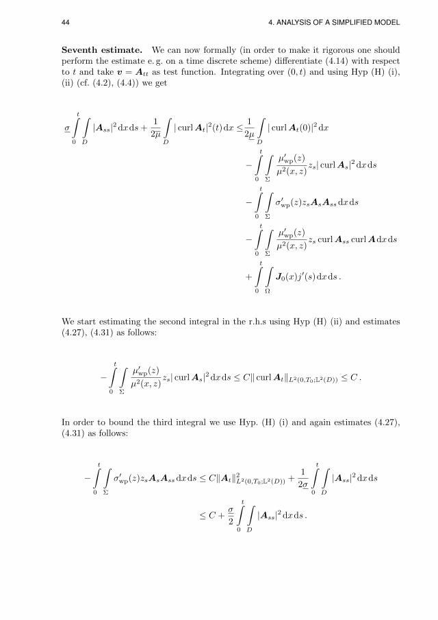
44 4. ANALYSIS OF A SIMPLIFIED MODEL
Seventh estimate. We can now formally (in order to make it rigorous one shouldperform the estimate e. g. on a time discrete scheme) differentiate (4.14) with respectto t and take v = Att as test function. Integrating over (0, t) and using Hyp (H) (i),(ii) (cf. (4.2), (4.4)) we get
σ
t∫0
∫D
|Ass|2 dxds+1
2µ
∫D
| curlAt|2(t)dx ≤ 1
2µ
∫D
| curlAt(0)|2 dx
−t∫
0
∫Σ
µ′wp(z)
µ2(x, z)zs| curlAs|2 dxds
−t∫
0
∫Σ
σ′wp(z)zsAsAssdxds
−t∫
0
∫Σ
µ′wp(z)
µ2(x, z)zs curlAss curlAdxds
+
t∫0
∫Ω
J0(x)j′(s)dxds .
We start estimating the second integral in the r.h.s using Hyp (H) (ii) and estimates(4.27), (4.31) as follows:
−t∫
0
∫Σ
µ′wp(z)
µ2(x, z)zs| curlAs|2 dxds ≤ C‖ curlAt‖L2(0,T0;L2(D)) ≤ C .
In order to bound the third integral we use Hyp. (H) (i) and again estimates (4.27),(4.31) as follows:
−t∫
0
∫Σ
σ′wp(z)zsAsAssdxds ≤ C‖At‖2L2(0,T0;L2(D)) +1
2σ
t∫0
∫D
|Ass|2 dxds
≤ C +σ
2
t∫0
∫D
|Ass|2 dxds .
4.4. Proof of the existence result 45
In the fourth integral we need to use the integration by parts formula, Hyp. (H) (ii),and estimates (4.27), (4.31), and (4.37):
t∫0
∫Σ
µ′wp(z)
µ2(x, z)zs curlAss curlAdxds
≤ Ct∫
0
‖ curlAs‖L2(D)‖ curlA‖L6(D)‖zss‖L3(Σ) ds+ C
t∫0
‖ curlAs‖2L2(D) ds
≤ Ct∫
0
‖ curlAs‖L2(D)‖zss‖L3(Σ) ds+ C
t∫0
‖ curlAs‖2L2(D) ds .
Now, we use Hyp. (H) (iii), (vi), estimate (4.35) with p = 3, and apply a standardGronwall lemma to the following inequality
σ
2
t∫0
∫D
|Ass|2 dxds+1
2µ
∫D
| curlAt|2(t)dx ≤ C + C
t∫0
‖ curlAs‖L2(D)‖zss‖L3(Σ) ds ,
getting the desired estimate
‖Att‖L2(0,T0;L2(D)) + ‖ curlAt‖L∞(0,T0;L2(D)) ≤ C . (4.38)
and so, since |At|2 ∈ L∞(0, T0;L3(D)), using [46], we get
‖θ‖L∞(Σ×(0,T0)) ≤ C . (4.39)
Collecting estimates (4.27), (4.31), (4.32), (4.36)–(4.39), we can now extend the solu-tion we found on [0, T0] to the whole time interval [0, T ]. Finally, notice that testing(4.15) by −θ−, where [ · ]− denotes the negative part, and using the assumptions on L,Hyp. (H) (vi) together with Hyp. (H) (v), (vi), we gain the non-negativity of θ. Thisconcludes the proof of existence of solutions to Problem (P).
4.4.3. Stability estimate
In this section we prove the stability estimate (4.20), entailing, in particular, unique-ness of solutions to Problem (P). Consider the time derivative of equation (4.14) andrewrite it in the following form∫
G
(h(x, z, zt)At + σ(x, z)Att) ·vdx
+
∫D
(1
µ(x, z)curlAt + `(x, z, zt) curlA
)· curlvdx =
∫Ω
j′(t)J0(x) ·vdx ,
(4.40)

46 4. ANALYSIS OF A SIMPLIFIED MODEL
for all v ∈ X and a.e. in (0, T ), where
h(x, z, zt) := σ′(x, z)zt, `(x, z, zt) :=µz(x, z)ztµ2(x, z)
.
Let (Ai, θi, zi), i = 1, 2, denote two triples of solutions corresponding to the data(A0,i, θ0,i, ji). Take the difference of (4.40) for the two triples i = 1, 2 and take thetest function v = At := (A1−A2)t. Then, denoting by z := z1−z2, we get, integratingover (0, t)
σ
2
∫G
|At(t)|2 dx+1
µ
t∫0
∫D
| curl As|2 dxds
≤ σ
2
∫G
|At(0)|2 dx+ Cσ
t∫0
(‖z‖L∞(Σ) + ‖zs‖L∞(Σ)
)‖As‖2L2(D) ds
+ Cσ
t∫0
(‖As‖2L2(D) + ‖z‖L∞(Σ)‖A1,ss‖L2(D)‖As‖L2(D)
)ds
+ Cµ
t∫0
(‖z‖L∞(Σ) + ‖zs‖L∞(Σ)
)‖As‖2L2(D) ds
+ Cµ
t∫0
(‖ curl A‖L2(D)‖As‖L2(D) + ‖z‖L∞(Σ)‖ curl As‖L2(D)
)ds
+ C
t∫0
|j′1 − j′2|‖As‖L2(D) ds,
(4.41)
where we have used the following inequalities (holding true for a.e. x) due to Hyp. (H)(i), (ii):
|h(x, z1, z1,t)− h(x, z2, z2,t)| ≤ Cσ (|z1,t||z1 − z2|+ |z1,t − z2,t|) ,|h(x, z2, z2,t| ≤ Cσ|z2,t| ,|`(x, z1, z1,t)− `(x, z2, z2,t)| ≤ Cµ (|z1 − z2||z1,t|+ |(z1 − z2)t|) ,|`(x, z2, z2,t| ≤ Cµ|z2,t| .

4.4. Proof of the existence result 47
Test now the difference of (4.15) for i = 1, 2 by θ := θ1 − θ2, integrate over (0, t), anduse the following inequalities
‖z‖L∞(Σ) +
t∫0
‖zs‖L∞(Σ) ds ≤ Ct∫
0
‖θ‖L∞(Σ) ds ≤ Ct∫
0
‖θ‖W 2,3/2(Σ) ds (4.42)
≤ Ct∫
0
(‖|A1,s|2 − |A2,s|2‖L3/2(D) + ‖zs‖L2(Σ)
)ds
≤ Ct∫
0
((‖A1,s‖L6(D) + ‖A2,s‖L6(D)
)‖As‖L2(D) + ‖θ‖L2(Σ)
)ds ,
obtaining (for all positive δ)
‖θ(t)‖2L2(Σ) +
t∫0
‖∇θ‖2L2(Σ) ds ≤ C‖θ(0)‖2L2(Σ)
+ δ
t∫0
‖θ‖2L6(Σ) ds+Cδ
t∫0
(‖θ‖2L2(Σ) +
(‖A1,s‖L6(D) + ‖A2,s‖L6(D)
)‖As‖L2(D)
)ds.
(4.43)
Add now the term∫ t
0‖θ‖2L2(Σ) to both sides of (4.43), choose δ sufficiently small and
add the result up to (4.41), one obtains (for all positive constant η)
‖At(t)‖2L2(D) +
t∫0
‖ curl As‖2L2(D) ds+ ‖θ(t)‖2L2(Σ) +
t∫0
‖θ‖2H1(Σ) ds (4.44)
≤ C‖At(0)‖2L2(D) + C‖ curl A(0)‖2L2(D) + C‖θ(0)‖2L2(Σ) + C
t∫0
|j1(s)− j2(s)|2 ds
+ η
t∫0
‖ curl As‖2L2(D) ds+ Cη
t∫0
‖θ‖2L2(Σ) ds
+ Cη
t∫0
(‖A1,s‖2L6(D) + ‖A2,s‖2L6(D) + ‖A1,ss‖2L2(D)
)‖As‖2L2(D) ds ,
where once more (4.42) has been used. Choosing now η sufficiently small in (4.44) andapplying a standard Gronwall lemma together with the regularity properties (4.11) ofthe solution, we obtain the desired stability estimate (4.20). This concludes the proofof Theorem 1.


Chapter 5.
Numerical solution of the inductionhardening problem
Introduction
In Chapter 4 the existence and uniqueness of solutions for a simplified induction hard-ening problem was established, where the material parameters depend only on thephase fraction z. In this chapter, the numerical solution of the full nonlinear problemis considered. Summarizing again, the induction hardening problem consists of find-ing functions A(x, t), θ(x, t) and z(x, t) that satisfy the following system of partial andordinary differential equations
σ∂A
∂t+ curl
1
µcurlA = Jsrc in D
ρcp∂θ
∂t− div κ∇θ = σ
∣∣∣∣∂A∂t∣∣∣∣2 − ρL∂z∂t in Σ
∂z
∂t=zr(θ)
τ(θ)[zeq(θ)− z]+ in Σ
(5.1)
for t ∈ (0, T ), where Jsrc and L denote the source current and the latent heat asintroduced in (3.17) and (3.34). As initial and boundary conditions we impose
A× n = 0 on ∂D, κ∇θ ·n+ ηθ = g on ∂Σ,
A(x, 0) = A0(x) in D, θ(x, 0) = θ0(x) and z(0) = 0 in Σ.(5.2)
The numerical solution process poses different challenges. The problem comprisesof nonlinear, coupled equations in the time domain that exhibit different time scales.Furthermore, due to the skin effect, the eddy current density concentrates in a smallboundary layer of the workpiece, which has to be resolved by the spatial discretization.Consequently, the problem also exhibits different length scales that will be resolved byadaptively generated grids using residual based error estimators.
The electromagnetic fields satisfy certain continuity conditions, they possess onlytangential continuity. This must be reproduced by the numerical scheme. For thediscretization of the curl-curl equation, the finite element method using edge elementsis utilized.
49

50 5. NUMERICAL SOLUTION OF THE INDUCTION HARDENING PROBLEM
The induction heating model represent an evolutionary problem. The common ap-proach is to discretize the equations with respect to space and with respect to timeseparately. At first, the equations are discretized in space by a Galerkin method. Thisis presented in Section 5.1 and 5.2. As a result one obtains a system of ordinary differ-ential equations, which is continuous in time. The discretization with respect to timeis considered in Section 5.3.
5.1. Discretization in space by the Galerkin method
The basic concept of the Galerkin method can be summarized as follows. Independentof the specific problem to solve, it consist of the following steps:
(i) The equations are considered as a variational problem.
(ii) One searches for the solution on a finite dimensional domain Vh that is equippedwith a basis ϕ1, . . . , ϕN. The fields of interest, e. g. the temperature θ(x, t),are expressed by a linear combination of the basis functions by the ansatz
θ(x, t) =N∑i=1
θi(t)ϕi(x).
(iii) For the Galerkin method, the test functions for the variational formulation arechosen as the basis functions. There results a system of equations that has to besolved by suitable methods to determine the unknown coefficients θi.
The finite element method represents a special case of the Galerkin method, wherethe computational domain is decomposed into small subdomains Kj , e. g. triangles in2D or tetrahedrons in 3D. The basis functions are defined locally on the triangulationTh = Kjj∈I and have to satisfy certain conditions. The finite element method as aspecial Galerkin method will be explained in more detail in Section 5.2.
5.1.1. Introduction of the Galerkin method
The Galerkin method describes a procedure to solve the variational formulation corre-sponding to equation (5.1). It is assumed that for fixed time t ∈ (0, T ), the variationalformulation of the continuous problem (5.1) possesses a solution A(t) in some spaceW, θ(t) in V and z(t) in Z. Then it is the fundamental approach to find approximatesolutions Ah(t) in Wh, θh(t) in Vh and zh(t) in Zh with finite dimensional spacesconsisting of vector valued functions Wh to discretize the magnetic vector potentialand scalar valued functions Vh and Zh to discretize the temperature and the volumefraction of austenite with respect to space. For simplicity we will approximate θh andzh with the same set of functions, i. e. Vh = Zh.
Since the spaces Vh and Wh are finite dimensional, there exist basis functions suchthat
Vh = Zh = spanϕ1, . . . ϕN and Wh = spanψ1, . . .ψN. (5.3)

5.1. Discretization in space by the Galerkin method 51
The unknown discrete solutions for the fields of interest are then expressed by thebasis in terms of the following ansatz
θh(x, t) =N∑i=1
θi(t)ϕi(x), zh(x, t) =N∑i=1
zi(t)ϕi(x) and Ah =N∑i=1
Ai(t)ψi(x)
(5.4)with time dependent coefficients θi(t), zi(t), i = 1, . . . , N and Ai(t), i = 1, . . . , N .
In order to determine a discrete solution, the weak formulation corresponding toequation (5.1) is considered on the spaces Vh and Wh. In addition to the ansatzfunctions, the test functions for the weak formulation are also taken from the spacesVh and Wh, respectively.
In Chapter 4, the weak formulation of the vector potential equation was introduced,which is now adapted to the discrete setting. For a fixed time t ∈ (0, T ) we regardthe function x 7→ Ah(x, t) as an element of Wh and write Ah(t) ∈Wh. For variable t,we obtain a function t 7→ Ah(t) with values in Wh. The weak formulation of (5.1)1 isnow: Find Ah(t) ∈Wh such that the following equation holds, cf. equation (4.14)∫
D
σ∂tAh ·ψh dx+
∫D
µ−1 curlAh · curlψh dx =
∫D
Jsrc ·ψh dx (5.5)
for all ψh ∈ Wh and a.e. in (0, T ) with initial condition Ah(x, 0) = Ah,0(x) anddivAh,0 = 0.
While in Chapter 4 the gauging condition divA = 0 was included in the ansatzspace X, we drop this condition for the numerical solution. Instead, we introduce aregularization of the electric conductivity σ in non-conducting regions such that
σ = σNC in D\(Σ ∪ Ω) with 0 < σNC minσwp, σCu. (5.6)
It is assumed that the compatibility condition divJsrc = 0 holds and the initial datasatisfies divAh,0 = 0, cf. (3.4). Then, the condition divAh = 0 is automaticallysatisfied (in a weak sense). The essential boundary condition Ah×n = 0 on ∂D mustbe included in the definition of the space Wh.
By analogous considerations as for the vector potential, we obtain the weak form ofthe heat equation: Find θh(t) ∈ Vh such that∫
Σ
ρcp∂tθh ϕh dx+
∫Σ
κ∇θh · ∇ϕh dx+
∫∂Σ
ηθh ϕh da =
∫Σ
fh ϕh dx+
∫∂Σ
g ϕh da (5.7)
for all ϕh ∈ Vh and a.e. in (0, T ) with θh(x, 0) = θh,0(x). The expression fh =
σ∣∣∂Ah
∂t
∣∣2 − ρL∂zh∂t is used as abbreviation for the right hand side.For the discretization of the rate law for the phase fraction of austenite, several
strategies might be possible, either a projection of the rate law on the space Vh or theintroduction of a suitable interpolation operator. The projection of equation (5.1)3
onto the space Vh corresponds to a variational formulation.

52 5. NUMERICAL SOLUTION OF THE INDUCTION HARDENING PROBLEM
Later on, the finite element method is introduced and the discrete space Vh will bechosen as the standard P1-finite element space, where the degrees of freedom corre-spond to nodal values. In this case, an interpolation can be easily realized by evaluatingthe rate law at the nodes of the discretization. In Section 5.2.5 the discretization ofthe rate law is described in detail using the finite element interpolation operator.
In order to complete the weak formulation, the initial and boundary conditions(5.2) have to be included in a suitable way. Regarding the boundary conditions,natural boundary conditions enter directly in the weak formulation, as it is the casefor equation (5.7). Essential boundary conditions like Ah×n = 0 on ∂D are includedin the definition of the finite dimensional spaces Wh and Vh. The definition of thesespaces is considered later on.
The initial conditions that are defined for Ah, θh and zh on the spaces Wh and Vhmust be consistent with (5.2). This can be achieved by using projection operators onthe spaces Vh and Wh that account for the condition divAh,0 = 0, i. e.
Ah(x, 0) = ΠW(A0(x)), θh(x, 0) = ΠV (θ0(x)) and zh(x, 0) = 0, (5.8)
with suitable projection operators ΠV on Vh and ΠW on Wh, satisfying div(ΠWA) = 0for all A with divA = 0 at least in a weak sense.
The weak formulation introduced above has to hold for all ϕh ∈ Vh and ψh ∈ Wh.Since the spaces Vh and Wh are finite dimensional, the basis functions are used as testfunctions. Summarizing, the weak formulation of the induction hardening problem isthe following. We search for the functions Ah(t) ∈Wh, θh(t) ∈ Vh and zh(t) ∈ Vh asdefined by the ansatz (5.4) such that for t ∈ (0, T ) the following equations are satisfiedfor all j = 1, . . . , N and k = 1, . . . , N :∫
D
σ∂tAh ·ψj dx+
∫D
µ−1 curlAh · curlψj dx =
∫D
Jsrc ·ψj dx
∫Σ
ρcp∂tθh ϕk dx+
∫Σ
κ∇θh · ∇ϕk dx+
∫∂Σ
ηθh ϕj da =
∫Σ
f ϕk dx+
∫∂Σ
g ϕk da
∂tzh = IT
(zr(θh)h
τ(θh)[zeq(θh)− zh]+
)Ah(x, 0) = ΠW(A0(x)), θh(x, 0) = ΠV (θ0(x)) and zh(x, 0) = 0.
(5.9)The discretization of the rate law for the phase fraction zh using the interpolationoperator IT is described in detail in Section 5.2.5.
5.1.2. The semi-discretized problem
Introducing the ansatz functions (5.4) into the weak formulation given above, thereresults a nonlinear system of ordinary differential equations, which has to be solvedby suitable methods. The discretization with respect to time and the linearization ofthe resulting system is considered in Section 5.3.

5.1. Discretization in space by the Galerkin method 53
In the case of the heat equation one obtains a system of nonlinear ordinary differ-ential equations for the time dependent coefficients θi(t), i = 1, . . . , N , which can bewritten as
Dρc∂tθ + Sκθ = F . (5.10)
Underlined quantities denote the vector representing the ansatz function (5.4), i. e.
θ = θi(t)i=1,...,N with θh(x, t) =∑Ni=1 θi(t)ϕi(x). We introduced the matrices
Dρc = Dρc,ij with Dρc,ij =
∫Σ
ρcpϕi ϕj dx
Sκ = Sκ,ij with Sκ,ij =
∫Σ
κ∇ϕi · ∇ϕj dx+
∫∂Σ
ηϕi ϕj da.
(5.11)
The matrix Dρc denotes the mass matrix and Sκ the stiffness matrix. The right hand
side is abbreviated by a (nonlinear) vector F (A, θ, z) = Fj(A, θ, z)j=1,...,N with
Fj(A, θ, z) =
∫Σ
f(Ah, θh, zh)ϕj dx+
∫∂Σ
g ϕj da. (5.12)
For the vector potential Ah there results the following system of nonlinear ordinarydifferential equations for the time dependent coefficients Ai(t), i = 1, . . . , N
Mσ∂tA+KµA = J (5.13)
with A = Ai(t)i=1,...,N . The newly introduced matrices Mσ and Kµ refer to themass matrix (associated to Wh) and the curl-curl matrix. They are defined as
Mσ = Mσ,ij with Mσ,ij =
∫D
σψi ·ψj dx
Kµ = Kµ,ij with Kµ,ij =
∫D
µ−1 curlψi · curlψj dx.
(5.14)
The right hand side is a time dependent vector J(t) = Jj(t)j=1,...,N and is definedas
Jj(t) =
∫D
Jsrc(t) ·ψj dx. (5.15)
Summary of the semi-discretized system
Summarizing the equations discretized in space we have to solve the following (non-linear) system of ordinary differential equations to determine Ah(t) ∈Wh, θh(t) ∈ Vh

54 5. NUMERICAL SOLUTION OF THE INDUCTION HARDENING PROBLEM
and zh(t) ∈ Vh defined by(5.4) such that for t ∈ (0, T ) there holds
Mσ∂tA+KµA = J
Dρc∂tθ + Sκθ = F
∂tzh = IT
(zr(θh)h
τ(θh)[zeq(θh)− zh]+
) (5.16)
with the matrices and right hand sides introduced in (5.11), (5.12), (5.14) and (5.15).Equation (5.16)3 is discussed in detail in Section 5.2.5. While the boundary conditionsare included in the weak formulation and the definition of the ansatz space, the initialconditions are given by
Ah(x, 0) = ΠW(A0(x)), θh(x, 0) = ΠV (θ0(x)) and zh(x, 0) = 0. (5.17)
The main challenge for the Galerkin method is the definition of the finite dimensionalspaces Vh, Wh and the corresponding basis functions. As a special type of the Galerkinmethod, a popular approach is the finite element method, where the computationaldomain is decomposed into simple subdomains and the basis functions are definedlocally. They are only non-vanishing on a small number of subdomains, which leadsto sparse matrices (5.11) and (5.14). Introducing a time discretization and a suitablelinearization strategy, cf. Section 5.3, the resulting linear system of equations can beeffectively solved by direct or iterative methods. In the next section, an overview ofthe finite element method is presented and a definition of the previously introducedfinite dimensional spaces Vh and Wh is given.
5.2. An overview of the finite element method
The construction of the test- and ansatz-functions for the finite dimensional spacesVh and Wh is the content of this section. We use the finite element method, which isbased on a decomposition of the computational domain into simple subdomains and alocal definition of the basis functions.
The definition of the spaces Vh and Wh introduced in this section is motivated bythe fact that the weak formulation of a linear, continuous problem corresponding tothe single model components, equations (5.5) and (5.7), where the material parametersare constant, possess solutions in the Hilbert spaces W 1,2(Σ) = H1(Σ) and L2
curl(D) =H(curl, D). The notation H1(Σ) and H(curl, D) is standard in the literature for thecase p = 2 and used in the following.
As has been shown in Chapter 4 for a reduced, nonlinear induction hardening prob-lem with simplified material parameters, higher regularity or integrability of the solu-tion for the continuous problem is expected. In the case of the full nonlinear problemwith temperature dependent parameters, a derivation of existence and regularity re-sults is even more complicated, and a solution in H1(Σ) and H(curl, D) can not beexpected.
Nevertheless, for the discrete problem these spaces are taken as basic concept. Theuse of the notion of ‘conformity’ for the finite elements introduced in the following

5.2. An overview of the finite element method 55
sections refers to the spaces H1(Σ) and H(curl, D) as solution spaces for correspondinglinearized, decoupled, single model components. For the full nonlinear problem, thefinite element discretization introduced in the following might be considered as non-conforming, due to the fact that the relations Vh ⊂ V and Wh ⊂ W might not beestablished, where V and W denote the solution spaces of the continuous problem forthe temperature and the vector potential, respectively.
5.2.1. The spatial decomposition of the computational domain
To describe the finite element method we need some preliminary assumptions. As inChapter 4 it is assumed that the domains Ω,Σ and D are bounded and have ‘sufficientsmoothness’. For simplicity it is assumed in this chapter that the domains Ω,Σ andD are polyhedral.
The main idea of the finite element method as a special type of the Galerkin methodis the decomposition of the domain D into small subdomains Kj , e. g. triangles in 2Dor tetrahedrons in 3D, and a local definition of the basis functions. The decompositionof the domain D, denoted as triangulation Th = Kjj∈I , where I denotes an indexset, has to satisfy several conditions. The triangulation is assumed to be regular, i. e.it is a covering of the whole domain
D =⋃j∈I
Kj , (5.18)
the elements are non-overlapping and the intersection of the elements Kj is eitherempty, a point, a common edge or a common face (3D) of the element. We denotethe diameter of each element K ∈ Th as hK . Then, h = maxK∈Th hK is used as adiscretization parameter. In order to guarantee convergence of the method as the gridsize h tends to zero, further conditions like angle conditions must be satisfied. Fordetails we refer to the literature, e. g. [13, 33]. Together with the triangulation Th weassociate the set of all vertices V, the set of all edges E and the set of all faces F .Referring to a single element, we will use the subscript K, i. e. the set of all verticesbelonging to the element K is denoted by VK . A similar notation will be used forvertices belonging to an edge E ∈ E .
The heat equation is only considered in the workpiece, i. e. on the subdomain Σ.Since Σ ⊂ D, the previous assumptions hold for the domain Σ in the same way.
5.2.2. An abstract definition of a finite element
In order to introduce the finite element method in detail, we begin with the generaldefinition of a finite element. Following Ciarlet [17], a finite element is defined as atriple (K,P,Λ), where
(i) K ⊂ Rd is a bounded and closed set with nonempty interior and Lipschitz-continuous boundary, typically intervals (d = 1), triangles (d = 2) or tetrahe-drons (d = 3),
(ii) P is a finite dimensional space of functions on K, usually polynomials,

56 5. NUMERICAL SOLUTION OF THE INDUCTION HARDENING PROBLEM
(iii) Λ is the set of degrees of freedom, given as linear forms Ni : P → R, i =1, . . . , nK , defined over the space P .
We denote by nK the number of degrees of freedom on K, which is equal to thedimension of P .
Two important concepts for the construction of finite elements are unisolvency andconformity. A finite element (K,P,Λ) is said to be unisolvent, if specifying a valuefor each of the degrees of freedom in Λ uniquely determines a function in P . As aconsequence, one obtains the following characterization, [79].
Definition 5.1. The finite element is unisolvent if there exist functions ϕj ∈ P, j =1, . . . , nK such that
Ni(ϕj) = δij for i, j = 1, . . . , nK .
The set of functions ϕ1, . . . , ϕnK ⊂ P defines the nodal basis of the finite dimensionalspace P .
In order to describe conformity, we need to introduce the finite element inter-polant. Assume we have given an unisolvent finite element (K,P,Λ) and denote byϕ1, . . . , ϕnK the nodal basis of the space P . Then for any function v ∈ V , where Vdenotes some Hilbert-space, the local interpolant is defined as
IK(v) =
nK∑i=1
Ni(v)ϕi. (5.19)
The local interpolant IK is linear, there holds Ni(IK(v)) = Ni(v), i = 1, . . . , nK , forall v ∈ V and IK(v) = v for all v ∈ P , [14].
In order to define the global interpolant, we assume that the computational domainD is subdivided into small subdomains by the regular triangulation Th, compare (5.18),and each subdomain Kj is equipped with some shape functions Pj and degrees offreedom Λj such that (Kj , Pj ,Λj) forms a finite element. Then, the global finiteelement interpolant IT is defined elementwise by the local interpolants IKj such that
IT (v)|Kj = IKj (v) for all Kj ∈ Th. (5.20)
The concept of conformity states that the finite element approximation of a functionv ∈ V belongs to the space V itself:
Definition 5.2. A finite element is considered as conforming, if for some Hilbert spaceV of functions over the domain D and a triangulation Th of D there holds
IT (v) ∈ V for all v ∈ V. (5.21)
In this work, we consider finite element approximations on the spaces H1(Σ) andH(curl, D). Conforming finite element functions on these spaces are characterized bythe following properties, [79].
Lemma 5.3 (Conformity requirements for H1). Consider a domain Σ with atriangulation Th. Then a function v : Σ→ R belongs to H1(Σ) if and only if
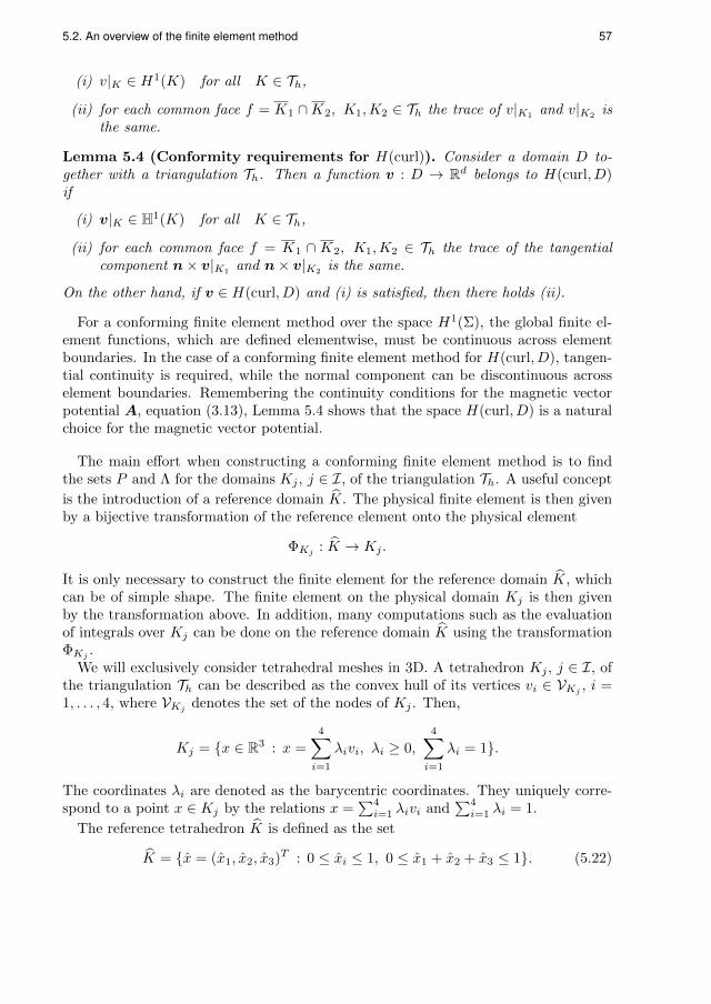
5.2. An overview of the finite element method 57
(i) v|K ∈ H1(K) for all K ∈ Th,
(ii) for each common face f = K1 ∩K2, K1,K2 ∈ Th the trace of v|K1and v|K2
isthe same.
Lemma 5.4 (Conformity requirements for H(curl)). Consider a domain D to-gether with a triangulation Th. Then a function v : D → Rd belongs to H(curl, D)if
(i) v|K ∈ H1(K) for all K ∈ Th,
(ii) for each common face f = K1 ∩ K2, K1,K2 ∈ Th the trace of the tangentialcomponent n× v|K1
and n× v|K2is the same.
On the other hand, if v ∈ H(curl, D) and (i) is satisfied, then there holds (ii).
For a conforming finite element method over the space H1(Σ), the global finite el-ement functions, which are defined elementwise, must be continuous across elementboundaries. In the case of a conforming finite element method for H(curl, D), tangen-tial continuity is required, while the normal component can be discontinuous acrosselement boundaries. Remembering the continuity conditions for the magnetic vectorpotential A, equation (3.13), Lemma 5.4 shows that the space H(curl, D) is a naturalchoice for the magnetic vector potential.
The main effort when constructing a conforming finite element method is to findthe sets P and Λ for the domains Kj , j ∈ I, of the triangulation Th. A useful concept
is the introduction of a reference domain K. The physical finite element is then givenby a bijective transformation of the reference element onto the physical element
ΦKj : K → Kj .
It is only necessary to construct the finite element for the reference domain K, whichcan be of simple shape. The finite element on the physical domain Kj is then givenby the transformation above. In addition, many computations such as the evaluationof integrals over Kj can be done on the reference domain K using the transformationΦKj .
We will exclusively consider tetrahedral meshes in 3D. A tetrahedron Kj , j ∈ I, ofthe triangulation Th can be described as the convex hull of its vertices vi ∈ VKj , i =1, . . . , 4, where VKj denotes the set of the nodes of Kj . Then,
Kj = x ∈ R3 : x =4∑i=1
λivi, λi ≥ 0,4∑i=1
λi = 1.
The coordinates λi are denoted as the barycentric coordinates. They uniquely corre-spond to a point x ∈ Kj by the relations x =
∑4i=1 λivi and
∑4i=1 λi = 1.
The reference tetrahedron K is defined as the set
K = x = (x1, x2, x3)T : 0 ≤ xi ≤ 1, 0 ≤ x1 + x2 + x3 ≤ 1. (5.22)
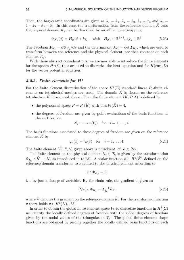
58 5. NUMERICAL SOLUTION OF THE INDUCTION HARDENING PROBLEM
Then, the barycentric coordinates are given as λ1 = x1, λ2 = x2, λ3 = x3 and λ4 =1− x1 − x2 − x3. In this case, the transformation from the reference domain K ontothe physical domain Kj can be described by an affine linear mapping
ΦKj (x) = BKj x+ bKj with BKj ∈ R3×3, bKj ∈ R3. (5.23)
The Jacobian FKj = ∂ΦKj/∂x and the determinant JKj = detFKj , which are used totransform between the reference and the physical element, are then constant on eachelement Kj .
With these abstract considerations, we are now able to introduce the finite elementsfor the spaces H1(Σ) that are used to discretize the heat equation and for H(curl, D)for the vector potential equation.
5.2.3. Finite elements for H1
For the finite element discretization of the space H1(Σ) standard linear P1-finite el-ements on tetrahedral meshes are used. The domain K is chosen as the referencetetrahedron K introduced above. Then the finite element (K, P,Λ) is defined by
• the polynomial space P = P1(K) with dimP1(K) = 4,
• the degrees of freedom are given by point evaluations of the basis functions atthe vertices, i. e.
Ni : v → v(Vi) for i = 1, . . . , 4.
The basis functions associated to these degrees of freedom are given on the referenceelement K by
ϕi(x) = λi(x) for i = 1, . . . , 4. (5.24)
The finite element (K, P,Λ) given above is unisolvent, cf. e. g. [86].The finite element on the physical domain Kj ∈ Th is given by the transformation
ΦKj : K → Kj as introduced in (5.23). A scalar function v ∈ H1(K) defined on thereference domain transforms to v related to the physical element according to
v ΦKj = v,
i. e. by just a change of variables. By the chain rule, the gradient is given as
(∇v) ΦKj = F−1Kj∇v, (5.25)
where ∇ denotes the gradient on the reference domain K. For the transformed functionv there holds v ∈ H1(K), [55].
In order to obtain the global finite element space Vh to discretize functions in H1(Σ)we identify the locally defined degrees of freedom with the global degrees of freedomgiven by the nodal values of the triangulation Th. The global finite element shapefunctions are obtained by piecing together the locally defined basis functions on each

5.2. An overview of the finite element method 59
element transformed to the physical domains Kj ∈ Th. Finally, the space Vh is definedas
Vh =⊕Vi∈V
spanϕi, (5.26)
where V denotes the set of vertices of the triangulation Th.Since the shape functions ϕi are defined by the barycentric coordinates, (5.24), the
shape functions are continuous across interelement boundaries. As a consequence,the constructed finite element space Vh is conforming with respect to H1(Σ), i. e.Vh ⊂ H1(Σ), cf. Lemma 5.3. With the finite element space as constructed above, thespace Vh consist of piecewise linear functions that are globally continuous and haveweak first derivatives [86],
Vh = v ∈ H1(Σ) : v|K ∈ P1(K) for all K ∈ Th. (5.27)
Higher order methods can be constructed in the same general framework. For detailswe refer to the literature, e. g. [17, 86].
5.2.4. Finite elements for H(curl)
In this section, we introduce the finite element discretization for the space H(curl, D).Due to the continuity properties of the electromagnetic fields arising in Maxwell’sequations, see Section 3.1.2, it is not appropriate to use vector valued finite elementspaces, whose components are discretized by finite elements for H1(D) as introducedabove.
The magnetic vector potential A for example has only continuous tangential com-ponents, cf. equation (3.13). In normal direction, jumps might occur at materialinterfaces. Consequently, using H1-finite elements, which provide continuity in allcomponents, would lead to computational errors. The discontinuity properties of thevector potentialAmust be considered in the construction of the finite element method.
The elements we define for the discretization of the vector potential equation goback on Nedelec [57, 58]. We will only consider lowest order Nedelec elements of firstand second kind.
Nedelec elements of first kind
The lowest order H(curl)-conforming finite element on the reference tetrahedron K isgiven by
• the polynomial space P = N0(K) defined by
N0(K) = a+ b× x : a, b ∈ R3, x ∈ K with dim(N0(K)) = 6 (5.28)
• and the edge based degrees of freedom
Nα : v →∫Eα
v · τ dx for α = 1, . . . , 6,

60 5. NUMERICAL SOLUTION OF THE INDUCTION HARDENING PROBLEM
where Eα, α = 1, . . . , 6 denotes the edges of the tetrahedron K and τ theuniquely defined tangential vector of the edge Eα.
The degrees of freedom refer to the integral of the tangential component of v. This isthe reason why Nedelec elements are often referred to as edge elements.
Regarding the polynomial degree of the space N0(K), it lies between the polynomialspaces of order 0 and 1, i. e. there holds
[P0(K)]3 ⊂ N0(K) ⊂ [P1(K)]3.
The space is constructed in such a way that the curl of the vector fields are piecewiseconstant functions, i. e.
curlN0(K) = [P0(K)]3.
The basis functions ψα associated to the edge based degrees of freedom Nα, α =1, . . . , 6 are given as follows, see e. g. [86],
ψ0α = λα2
∇λα1− λα1
∇λα2(5.29)
for each edge Eα ∈ EK connecting the vertices Vα1 and Vα2 and λαi denoting thebarycentric coordinate associated to the vertex Vαi . The tangential trace of the shape
function is constant on each edge of K, there holds
ψ0α · τEβ =
1
|Eβ |δαβ for edges Eα, Eβ ∈ EK , α, β = 1, . . . , 6.
As a consequence there holds Nβ(ψα) =∫Eαψ0α · τ dx = δαβ , i. e. the finite element
(K,N0(K),Λ) is unisolvent.
Nedelec elements of second kind
The Nedelec element of second kind extends the polynomial space to the full space ofpolynomials of degree at most one. It is defined by the following characterization.
• The polynomial space P = N1(K) is given by
N1(K) = [P1(K)]3 with dim(N1(K)) = 12, (5.30)
• the edge based degrees of freedom Λ are now represented by the following mo-ments on each edge Eα, α = 1, . . . , 6
Nkα : v →
∫Eα
v · τ qk dx for k = 0, 1,
where qk denotes a basis for P1(Eα) and q0 = 1.

5.2. An overview of the finite element method 61
The vector valued basis functions ψkα associated to the degrees of freedom Nkα, α =
1, . . . , 6 and k = 0, 1 for each edge Eα ∈ EK connecting the vertices Vα1 and Vα2 arenow given as
ψ0α = λα2
∇λα1− λα1
∇λα2
ψ1α = ∇(λα1λα1).
(5.31)
The functions ψ0α,ψ
1α form a basis for the lowest order Nedelec element of second
kind (K,N1(K),Λ), compare to [86].
Global shape functions
The shape functions defined above refer to the reference domain K. In order to obtainthe shape functions on the physical domains Kj ∈ Th, we use the transformation
(5.23). The transformation of a vector valued function w ∈ H(curl, K) is a bit more
involved than in the case of H1(K). Since curl∇v = 0 for v ∈ H1(K), we have
that ∇v ∈ H(curl, K). Consequently, a function w ∈ H(curl, K) should transformaccording to (5.25) in the following way
w ΦK = F−1K w.
The curl transforms according to
(curlw) ΦK =1
detFKFK(curlx w),
where curlx refers to the curl with respect to the reference domain K. As a conse-quence, there holds w ∈ H(curl,K) for w defined on the physical domain, comparee. g. [55].
In order to obtain the global finite element spaces W 0h and W 1
h consisting of Nedelecelements of first and second kind, respectively, we identify the locally defined degreesof freedom with the global degrees of freedom defined as the tangential traces along theedges of the triangulation Th. The global finite element shape functions are obtainedby piecing together the locally defined basis functions on each element transformed tothe physical domains Kj ∈ Th such that
W 0h =
⊕Ek∈E
spanψ0k (5.32)
for Nedelec elements of first kind and
W 1h =
⊕Ek∈E
spanψ0k,ψ
1k (5.33)
for Nedelec elements of second kind, where E denotes the set of edges of Th.The constructed finite element discretizations with Nedelec elements of first and
second kind are unisolvent and conforming with respect to H(curl, D). For a proof ofthis result we refer to the literature, e. g. [55, 57, 58].

62 5. NUMERICAL SOLUTION OF THE INDUCTION HARDENING PROBLEM
Since the degrees of freedom are defined as the tangential components along theedges of the triangulation, the global orientation of the tangential vectors of the edgeshas to be taken into account when considering the identification of the local andphysical degrees of freedom. Depending on the fact wether the tangential vectors inthe description of the reference element and the physical element have the same or theopposite orientation, the transformed shape functions have to be multiplied with +1or −1 when addressing the global shape functions.
Summarizing, the introduced H(curl)-conforming finite element spaces can be writ-ten as
W 0h = v ∈ H(curl, D) : v|K ∈ N0(K) for all K ∈ Th
W 1h = v ∈ H(curl, D) : v|K ∈ N1(K) for all K ∈ Th
with N0(K) and N1(K) introduced in (5.28) and (5.30), cf. [86].
As a result, we are now able to define the discrete spaces Vh and Wh for the Galerkinmethod. The space Vh is chosen as the standard linear P1-finite elements, compare(5.27). For the space Wh we choose either lowest order Nedelec elements of first orsecond kind. Nedelec elements of first kind are weakly divergence free, which hasadvantages in realizing the condition divAh = 0. For Nedelec elements of secondkind, the additional degrees of freedom provide a better approximation of the field Ah
itself. Essential boundary conditions must be included in the ansatz space, such thatwe define
Wh = vh ∈W kh : vh × n = 0 on ∂D
with k = 0 for lowest order Nedelec elements of first kind and k = 1 for lowest orderNedelec elements of second kind.
5.2.5. About the spatial discretization of the phase fraction
Having introduced the finite element method, the discretization of the volume fractionof austenite z is considered again. In the continuous setting there holds, cf. (5.1)
∂tz =zr(θ)
τ(θ)[zeq(θ)− z]+ in Σ for t ∈ (0, T ).
The discretized phase fraction zh was introduced by the ansatz zh =∑Ni=1 zi(t)ϕi(x),
where ϕ1, . . . , ϕN denotes the basis of Vh, compare to (5.4). The transition from zto zh is realized by the nodal interpolation operator IT introduced in Section 5.2.2:On each element it is defined as
IK(v) =
nK∑i=1
Ni(v)ϕi,
where Ni, i = 1, . . . , nK denote the local degrees of freedom on a single element K.This interpolation operator is extended to the whole domain by defining the global

5.3. Discretization in time and nonlinear behaviour 63
interpolation operator IT such that
IT (v)|Kj = IKj (v) for all Kj ∈ Th,
compare to (5.20). Consequently, the coefficients zi(t) correspond to the degrees offreedom Ni on each domain Kj ∈ Th, i. e. on Vh they represent the nodal values.
Since the interpolation operator is linear, we obtain from zh = IT (z) an analogousexpression for the time derivative of zh such that ∂tzh = IT (∂tz). Consequently, onthe discrete level there holds the following rate law for the volume fraction of austenite
∂tzh = IT (∂tz) = IT(zr(θ)
τ(θ)[zeq(θ)− z]+
). (5.34)
In order to evaluate the projection operator for the right hand side of the rate lawabove, we have to determine the nodal values on each element Kj ∈ Th. Since θ andz are discretized by linear P1-finite elements, this is realized by evaluating the righthand side of equation (5.34) for the nodal values of θh and zh such that for zh thereholds the following equation
∂tzi =zr(θi)i
τ(θi)[zeq(θi)− zi]+, i = 1, . . . , N, (5.35)
where θi(t) and zi(t) are the coefficients of the finite element functions θh(x, t) andzh(x, t), cf. (5.4).
5.3. Discretization in time and nonlinear behaviour
5.3.1. Discretization in time
The semi-discretized equations (5.16) are still continuous in time. They represent asystem of nonlinear ordinary differential equations, which has to be solved in time toobtain the time dependent finite element solution of the magnetic vector potential, thetemperature and the phase fraction of austenite. The nonlinear ODE system (5.16)can be written in the following general form
∂y
∂t= R(t, y), y(0) = y0, (5.36)
where y is the vector consisting of the finite element representations (A, θ, z). R(t, y)denotes the right hand side, which is obtained by the spatial discretization of thepartial differential equations and y0 denotes the initial solution. In order to solve suchkind of systems, a discretization with respect to time is necessary.
When using the finite element method to solve parabolic equations, the resultingordinary differential equations are stiff systems, [33]. In order to avoid very small timesteps, methods with certain stability properties should be used, e. g. A-stability, wherethe region of stability contains the complete left half-space of the complex plane [35].Methods that are A-stable are among many others the implicit Euler method, the

64 5. NUMERICAL SOLUTION OF THE INDUCTION HARDENING PROBLEM
midpoint rule, the α-method1 with α ≥ 1/2 and the Backward-Differential-Formula oforder two (BDF-2). The midpoint rule, the α-method with α = 1/2 and the BDF-2method approximate the time derivative with an accuracy of order two, while the othermethods are only of order one. In addition, the BDF-2 method is also L-stable, whichis a stronger property than A-stability. In this section, we introduce these methods tosolve the semi-discretized system (5.16) in time.
To explain the different methods, it is assumed that the whole time interval isdivided into equidistant time steps 0 < . . . < tk < . . . < T . The time derivative isapproximated by finite differences
∂y
∂t≈ yk+1 − yk
τ,
where τ = tk+1 − tk denotes the time step and yk = y(tk) .The α-method is defined by an interpolation of the right hand side R(t, y) evaluated
at times tk+1 and tk. The integration of equation (5.36) is obtained by solving thefollowing scheme for yk+1
yk+1 − yk
τ= αR(tk+1, yk+1) + (1− α)R(tk, yk). (5.37)
The parameter α is used to control the implicit behaviour of the solution method fromexplicit (α = 0) to fully implicit. For α = 1 there results the implicit Euler method,the case α = 1/2 corresponds to the Crank-Nicolson scheme [19].
The BDF-2 method is a two-step method, see e. g. [35]. Computing the new iterateyk+1 involves the previous two time steps by solving the time stepping scheme
3yk+1 − 4yk + yk−1
2τ= R(tk+1, yk+1). (5.38)
The Crank-Nicolson method and the BDF-2 method approximate the time derivativewith order two. Since the time derivative of the magnetic vector potential is used toevaluate the Joule heat, Q = σ |∂tA|2, we are interested in an accurate approximationof this term and we use the BDF-2 method to solve the vector potential equation intime. Since this method represents a multistep method, two initial values are necessary,which are generated consistently by the Crank-Nicolson method.
5.3.2. Nonlinearities
The methods above are implicit (except for α = 0), the nonlinear right hand sidehas to be evaluated at the actual time step tk+1 and at yk+1 = y(tk+1), which is theunknown quantity. Suitable methods have to be used to resolve these nonlinearities.
Typically, Newton type methods are used to solve nonlinear equations. For this, wewrite the integration schemes (5.37) or (5.38) in the form
F (yk+1) = 0. (5.39)
1In literature, the α-method is usually denoted as θ-method. Since we denote the temperature byθ, we use the parameter α instead.

5.3. Discretization in time and nonlinear behaviour 65
The Newton method is typically derived by linearizing equation (5.39) with respect tosome known value y, i. e.
F (yk+1) ≈ F (y) +∇F (y) (yk+1 − y),
where∇F (y) denotes the derivative of F with respect to yk+1 evaluated at y. Denotingδy = (yk+1 − y) as the update increment, we can write the Newton algorithm tocompute yk+1 using the solution at the actual time step yk as initial value as follows.
(i) Define an initial value y = yk,
(ii) solve the linear system ∇F (y) δy = −F (y),
(iii) update yk+1 = y + δy,
(iv) go to step (ii) with y = yk+1 and iterate until some stopping criterion is satisfied,e. g. ‖δy‖ ≤ ε.
Often in application, only a fixed number of Newton steps, in the simplest case onlyone Newton step, is performed to compute the solution at the new time step yk+1
using the iterate yk as initial guess. The Newton method converges super-linearly,provided the initial guess is close to the exact solution. We refer to the literature fora convergence analysis, e. g. [20].
The complicated task is to evaluate the Jacobian matrix ∇F . Since the material pa-rameters depend nonlinearly on the unknown temperature, phase fraction and even themagnetic vector potential, the computation of the derivative involves also the deriva-tive of the stiffness and mass matrix (5.11) and (5.14) with respect to the unknowns(A, θ, z). The solution of the nonlinear system by Newton’s method consisting of therepeatedly evaluation of the Jacobian matrix ∇F and the iteration algorithm givenabove is computational quite expensive.
We want to avoid the iterative solution by the Newton method and propose a semi-implicit algorithm. With this method, the right hand side R(t, y) in (5.36) is onlyevaluated implicitly at time tk+1 for linear terms. Nonlinear terms, especially thematerial parameters, are evaluated at the old time step tk. This is also comparable tothe method of freezing coefficients, see e. g. [33].
Considering the vector potential equation (5.13) discretized by the Crank-Nicolsonscheme in time leads to the following system
Mσ(Ak+1 −Ak) = −τ2Kµ(Ak+1 +Ak) +
τ
2(Jk+1 + Jk),
where the matricesMσ andKµ, cf. (5.14), are assembled with the material parametersevaluated at time tk. Since the source current density depends only on time, we defineJk+1 = Jj(tk+1)j with Jj(t
k+1) =∫DJsrc(tk+1) ·ψj dx. In each time step, we have
to solve the following linear system(Mσ +
τ
2Kµ
)Ak+1 =
(Mσ −
τ
2Kµ
)Ak +
τ
2(Jk+1 + Jk). (5.40)
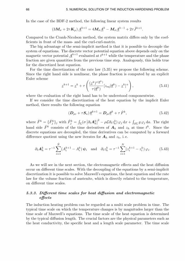
66 5. NUMERICAL SOLUTION OF THE INDUCTION HARDENING PROBLEM
In the case of the BDF-2 method, the following linear system results
(3Mσ + 2τKµ)Ak+1 = 4MσAk −MσA
k−1 + 2τ Jk+1.
Compared to the Crank-Nicolson method, the system matrix differs only by the coef-ficients in front of the mass- and the curl-curl-matrix.
The big advantage of the semi-implicit method is that it is possible to decouple thesystem of equations. The discrete vector potential equation above depends only on themagnetic vector potential Ak+1 evaluated at tk+1 while the temperature and the phasefraction are given quantities from the previous time step. Analogously, this holds truefor the discretized heat equation.
For the time discretization of the rate law (5.35) we propose the following scheme.Since the right hand side is nonlinear, the phase fraction is computed by an explicitEuler scheme
zk+1 = zk + τ
((zk)r(θ
k)
τ(θk)[zeq(θk)− zk]+
), (5.41)
where the evaluation of the right hand has to be understood componentwise.If we consider the time discretization of the heat equation by the implicit Euler
method, there results the following equation
(Dρc + τSκ) θk+1 = Dρcθk + τ F k, (5.42)
where F k = F kj j with F kj =∫
Σ(σ∣∣∂tAk
h
∣∣2 − ρL∂tzkh)ϕj dx+∫∂Σg ϕj da. The right
hand side F k consists of the time derivatives of Ah and zh at time tk. Since thediscrete equations are decoupled, the time derivatives can be computed by a forwarddifference quotient using the new iterates for Ah and zh, i. e.
∂tAkh = τ−1
N∑i=1
(Ak+1i −Aki )ψi and ∂tz
kh = τ−1
N∑i=1
(zk+1i − zki )ϕi. (5.43)
As we will see in the next section, the electromagnetic effects and the heat diffusionoccur on different time scales. With the decoupling of the equations by a semi-implicitdiscretization it is possible to solve Maxwell’s equations, the heat equation and the ratelaw for the volume fraction of austenite, which is directly related to the temperature,on different time scales.
5.3.3. Different time scales for heat diffusion and electromagneticeffects
The induction heating problem can be regarded as a multi scale problem in time. Thetypical time scale on which the temperature changes is by magnitudes larger than thetime scale of Maxwell’s equations. The time scale of the heat equation is determinedby the typical diffusion length. The crucial factors are the physical parameters such asthe heat conductivity, the specific heat and a length scale parameter. The time scale
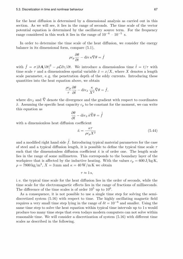
5.3. Discretization in time and nonlinear behaviour 67
for the heat diffusion is determined by a dimensional analysis as carried out in thissection. As we will see, it lies in the range of seconds. The time scale of the vectorpotential equation is determined by the oscillatory source term. For the frequencyrange considered in this work it lies in the range of 10−6 – 10−5 s.
In order to determine the time scale of the heat diffusion, we consider the energybalance in its dimensional form, compare (5.1),
ρcp∂θ
∂t− div κ∇θ = f
with f = σ |∂A/∂t|2 − ρL∂z/∂t. We introduce a dimensionless time t = t/τ withtime scale τ and a dimensionless spatial variable x = x/X, where X denotes a lengthscale parameter, e. g. the penetration depth of the eddy currents. Introducing thesequantities into the heat equation above, we obtain
ρcpτ
∂θ
∂t− divx
κ
X2∇θ = f ,
where divx and ∇ denote the divergence and the gradient with respect to coordinatesx. Assuming the specific heat capacity cp to be constant for the moment, we can writethis equation as
∂θ
∂t− divx κ∇θ =
ˆf
with a dimensionless heat diffusion coefficient
κ =κτ
ρcpX2(5.44)
and a modified right hand sideˆf . Introducing typical material parameters for the case
of steel and a typical diffusion length, it is possible to define the typical time scale τsuch that the dimensionless diffusion coefficient κ is of order one. The length scalelies in the range of some millimetres. This corresponds to the boundary layer of theworkpiece that is affected by the inductive heating. With the values cp = 600 J/kg K,ρ = 7800 kg/m3, X = 3 mm and κ = 40 W/m K we obtain
τ ≈ 1 s,
i. e. the typical time scale for the heat diffusion lies in the order of seconds, while thetime scale for the electromagnetic effects lies in the range of fractions of milliseconds.The difference of the time scales is of order 105 up to 106.
As a consequence, it is not possible to use a single time step for solving the semi-discretized system (5.16) with respect to time. The highly oscillating magnetic fieldrequires a very small time step lying in the range of δt = 10−6 and smaller. Using thesame time step to solve the heat equation within typical time intervals up to 1 s wouldproduce too many time steps that even todays modern computers can not solve withinreasonable time. We will consider a discretization of system (5.16) with different timescales as described in the following.

68 5. NUMERICAL SOLUTION OF THE INDUCTION HARDENING PROBLEM
5.3.4. Time discretization of the coupled system
Introduction of different time steps
Since the heat conduction and the electromagnetic effects exhibit different time scales,it is the aim to decouple system (5.16) and solve the time dependent equations withdifferent time step sizes, as it is the usual approach for induction heating problems inthe time domain, [18].
If we consider the vector potential equation (5.1)1 for a given temperature θ, then itrepresents a parabolic equation that possesses a time periodic solution due to the timeperiodic source term. We solve this equation for some periods using a time steppingscheme with time step size δt.
The heat equation (5.1)2 also represents a parabolic equation with rapidly varying
right hand side σ |∂tA|2. As we have seen, the temperature changes at a time scale thatis much larger than the one of the right hand side, which is governed by the frequencyof the source current. The usual approach is to approximate the Joule heat term byits average over one period, [18]. Then, the heat equation can be solved using timesteps ∆t δt, where the oscillating Joule heat is replaced by an averaged Joule heatterm, which is obtained from the periodic solution of the vector potential equation.For a further justification of this approach, see also Appendix A.3.
We formulate the algorithm following [18]. We consider the time interval (0, T ) anddecompose it into M equal time steps tk with time step size ∆t = T/M such that
tk = k∆t for k = 1, . . . ,M.
The ‘large’ time step size ∆t results from the typical time scale of the heat conduction.We obtain time intervals (tk, tk+1), k = 0, . . . ,M − 1, on which we solve the electro-magnetic problem with the assumption that the temperature is constant. For this weuse a time step δt ∆t that is related to the source term of the vector potentialequation. We obtain a decomposition of the intervals (tk, tk+1) such that
tk,l = tk + lδt for l = 0, 1, . . .
and solve the vector potential equation by the time stepping scheme introduced inSection 5.3.2. In general, it is not necessary to solve for Ah on the whole interval(tk, tk+1). Since the source term Jsrc is periodic, the discrete solution Ah is periodicsuch that it is sufficient to solve until a periodic solution is obtained. This is realizedby solving the vector potential equation for a fixed number of periods. Numericaltests using the L-stable BDF-2 time stepping method have shown that a periodicvector potential Ah is obtained after two, at most three periods. As an alternative, aperiodicity test can be used to verify that the solution Ah is periodic.
The Joule heat, which enters the right hand side of the heat equation, is obtainedby averaging the term σ |∂tAh|2 over one period,
Q =ω
2π
2πω∫
0
σ |∂tAh|2 dt. (5.45)

5.3. Discretization in time and nonlinear behaviour 69
The averaged Joule heat Q is still time dependent due to the temperature and phasedependent electrical conductivity σ(θ, z), but it is not highly oscillating any more. Fi-nally, we have decoupled the vector potential equation and the heat equation togetherwith the rate law for the phase fraction. Having determined the averaged Joule heat,the heat equation can be solved by a suitable time stepping scheme at the discretetimes tk, k = 1, . . . ,M .
As a test of periodicity it is suggested in [18] not to compare values of the magneticvector potential Ah but to check the periodicity of the magnetic vector potential interms of the Joule heat Q = σ |∂tAh|2 evaluated at a time step tk,l, denoted by Q1
and one period later, denoted by Q2. Then, the authors define quantities
ηi =|Q2,i −Q1,i|‖Q2‖
that are evaluated at all points i of the mesh. If the values ηi are below some threshold,then the solution is assumed to be periodic and the averaged Joule heat Q is acceptedfor the computation of the next temperature time step. Otherwise, the time iterationof the vector potential equation is carried out for one more period.
The question that arises with this method is, for which points xi of the mesh thetest is performed. This question is closely related to the fact, how and where the Jouleheat
Q = σ
∣∣∣∣∂Ah
∂t
∣∣∣∣2 ,respectively the averaged Joule heat Q, is evaluated. Since the discrete vector potential
is given as Ah(x, t) =∑Nj=1Aj(t)ψj(x), where Aj are the tangential components of
Ah along the edges Ej ∈ E of the triangulation Th, it is hardly possible to express
the components of the modulus |A| = (|Ax|2 + |Ay|2 + |Az|2)1/2 by the finite elementrepresentation vector A itself. Therefore, in order to compute the Joule heat, it isnecessary to evaluate the components of the vector field Ah(x, t) at finitely manypoints xi in space, which involves the evaluation of the components of the vectorvalued basis functions ψj(x) in space. Consequently, one has to specify points xi atwhich the Joule heat is evaluated.
One possibility is to evaluate Q at the nodes of the triangulation Th. In this way, itis easily possible to obtain a finite element interpolant of Q with respect to the spaceVh. But since the vector potential Ah might be discontinuous in normal direction atinterelement boundaries, this method is connected with approximation errors.
The Joule heat appears at the right hand side of the weak formulation of the heatequation, consisting of the evaluation of integrals like
Fj =
∫Σ
(Q− ρL∂tzh)ϕj dx+
∫∂Σ
g ϕj da,
compare (5.12). Typically in numerical implementations of finite element methods,quadrature formulas are used to compute integrals by evaluating the integrand atcertain quadrature points. Therefore, the averaged Joule heat is computed at the

70 5. NUMERICAL SOLUTION OF THE INDUCTION HARDENING PROBLEM
quadrature points qi that are also used to evaluate the integrals above during theassembly of the right hand side of the space discretized heat equation. With thismethod, a higher accuracy than for the evaluation of Q at the nodes of Th is expected.The periodicity test described above can be performed for the values at the quadraturepoints, too.
5.3.5. On the existence of solutions for the discretized system
In this section, we consider the existence of solutions for the fully discretized andlinearized problem consisting of equations (5.40), (5.41) and (5.42). We search for asolution at the fixed time tk+1 assuming that a solution for the previous time step tk
is known. The existence and uniqueness of discrete solutions for the heat equation isa common result. For the phase fraction zh it can be obtained by standard results onODEs. Due to the non-trivial kernel of the curl-operator, i. e.
ker(curl) := v ∈ H(curl, D) : curlv = 0 = ∇H1(D),
the existence of a unique solution for the discretized vector potential Ah is not trivial.The foundation is the general theory for the existence and uniqueness of solutions
for elliptic problems on some Hilbert space S in terms of the following result.
Lemma 5.5 (Lax-Milgram, [33]). Let a( · , · ) : S×S → R be a bounded, S-ellipticbilinear form. Then for every f ∈ S∗ the variational equation
a(u, v) = f(v) for all v ∈ S
possesses a unique solution u ∈ S. Furthermore, there holds the a priori estimate
‖u‖S ≤1
γ‖f‖S∗ .
We apply the general theory to the fully discretized equation (5.40), where the vectorpotential equation is discretized by the Crank-Nicolson method (the same results holdtrue for the BDF-2 method). With the definition of the matrices (5.11) this problemis equivalent to
a(Ak+1h ,wh) = f(wh) for all wh ∈Wh, (5.46)
where the bilinear form a : Wh ×Wh → R is defined as
a(Ah,wh) =
∫D
σAh ·wh dx+τ
2
∫D
µ−1 curlAh · curlwh dx
and the linear functional f ∈ H(curl, D)∗ is given by
f(wh) =
∫D
σAkh ·wh dx− τ
2
∫D
µ−1 curlAkh · curlwh dx
+τ
2
∫D
(Jsrc(tk+1) + Jsrc(tk)) ·wh dx.

5.3. Discretization in time and nonlinear behaviour 71
One has to show the boundedness and the coercivity of the bilinear form a( · , · ), i. e.|a(u, v)| ≤ M ‖u‖S ‖v‖S for all u, v ∈ S with some constant M > 0 and a(u, u) ≥γ ‖u‖2S for all u ∈ S with a constant γ > 0
Since the material parameters are evaluated at the previous time step, they representknown quantities depending on space x. As in Chapter 4 the coefficients σ and µ areassumed to be bounded from above and below, cf. Hyp. (H) (i) and (ii). Rememberthat instead of including the gauging condition divAh into the definition of the ansatzspace Wh, a regularization of the electrical conductivity is introduced, i. e. σ = σNC
in D\(Σ ∪ Ω) with 0 < σNC minσwp, σCu, cf. (5.6). Then, for the bilinear forma( · , · ) there holds
a(Ah,wh) =
∫D
σAh ·wh dx+τ
2
∫D
µ−1 curlAh · curlwh dx
≤ σ ‖Ah‖L2 ‖wh‖L2 +τ
2µ−1 ‖curlAh‖L2 ‖curlwh‖L2
≤ maxσ, τ2µ−1 ‖Ah‖curl ‖wh‖curl
for all Ah,wh in Wh ⊂ H(curl, D) equipped with the usual norm on H(curl, D). Onthe other hand, there holds
a(wh,wh) =
∫D
σwh ·wh dx+τ
2
∫D
µ−1 curlwh · curlwh dx
≥ σ ‖wh‖2L2 +τ
2µ−1 ‖curlwh‖2L2
≥ minσ, τ2µ−1 ‖wh‖2curl
for all wh in Wh. Consequently, the bilinear form a( · , · ) is bounded and coercive onWh. In the case of σ = 0 in non-conducting regions, coercivity can not be established,since for arbitrary gradient fields ∇φ there holds a(∇φ,∇φ) = 0 on D\(Σ ∪ Ω), but‖∇φ‖curl = ‖∇φ‖L2 . In this case, the gauging condition divAh is necessary. Coercivitycan be established for a mixed variational problem, cf. [86].
From Lemma 5.5 one obtains that the discrete equation (5.40) possesses a uniquesolution, provided the right hand sides are sufficiently regular. Assuming Jsrc ∈ L2(D),then there holds f ∈ L2(D). Consequently, we have the existence of a unique discretesolution Ak+1
h at the new time step tk+1.
5.3.6. Solution of the linearized systems
In every time step, the time stepping schemes introduced above require the solutionof linear systems in the form
Su = b,
where S = (Mσ + τ/2Kµ) in the case of the vector potential equation discretizedby the Crank-Nicolson scheme, S = (3Mσ + 2τKµ) for the BDF-2 method, or S =

72 5. NUMERICAL SOLUTION OF THE INDUCTION HARDENING PROBLEM
(Dρc+τSκ) for the heat equation discretized by an implicit Euler scheme, with variousright hand sides b. In order to solve these linear systems, direct as well as iterativemethods are used.
The heat equation is solved only in the workpiece, the domain Σ. Compared tothe vector potential equation, which has to be solved on the whole domain D and isdiscretized by edge elements, it is possible to use a direct solver. We use the directsparse solver PARDISO.
The package PARDISO is a high-performance, robust, memory efficient and easy touse software for solving large sparse symmetric and non-symmetric linear systemsof equations on shared-memory and distributed-memory architectures. PARDISOcalculates the solution of a set of sparse linear equations with multiple right-handsides using a parallel LU , LDL or LLT factorization, [66, 67].
For huge systems, direct solvers come to their limits regarding memory usage andcomputational time. The use of iterative methods, such as the preconditioned con-jugate gradient method (PCG) is suggested. For solving Maxwell’s equation, theperformance of the PCG method with a simple Jacobi preconditioner is due to theill-conditioned iteration matrix and the non-trivial kernel of the curl-operator quitebad. Special methods like additive Schwarz-methods [86] or multigrid methods [37]are proposed. Their implementation is quite complex.
As an alternative, we use a combination of the direct, high-performance solver PAR-DISO and the PCG method. Solving the vector potential equation, we have to solvesystems Su = b with varying right hand sides b. In Section 5.5, we introduce an av-eraging method to linearize the vector potential equation. With this method, we candrop the nonlinear dependence of the magnetic permeability µ on the magnetic field.Then, the iteration matrix S = (Mσ + τ/2Kµ) does not change during a time step ∆tand we propose the following method. We solve the system Su = b using PARDISOonce and store the LU or LLT -decomposition of S. Then, it is easily possible to solvethe system for various right hand sides b.
In the next time step for the heat equation, tk + ∆t, the matrices Mσ,Kµ andconsequently the iteration matrix S need to be reassembled. The changes result fromthe changing temperature, since the material parameters depend on the temperature.If the changes in the temperature θ are small, the differences in σ and µ compared tothe previous time step are small. Consequently, the difference between the iterationmatrix for subsequent time steps is small. This suggests the use of the LU or LLT
decomposition of the previous time step as preconditioner for a PCG method. This issimilar to incomplete Cholesky CG-methods (ICCG) that use an incomplete or inexactCholesky decomposition of the iteration matrix as a preconditioner.
In the following, we give a sketch of the PCG method. In order to solve the lin-ear system Su = b, where S is a symmetric, positive definite matrix, the systemC−1Su = C−1b is considered, where C denotes the preconditioner. The PCG methodis explained e. g. in [33] and consist of the following steps.

5.4. Adaptive mesh generation 73
• Starting from an initial value u0 ∈ Rn define vectors
p0 = d0 = b− Su0 and s0 = C−1d0.
• Compute recursively for k = 0, 1, . . . until∥∥dk∥∥ ≤ ε
αk =(sk, dk)
(Spk, pk)
uk+1 = uk + αkpk
dk+1 = b− Suk+1
sk+1 = C−1dk+1
βk =(sk+1, dk+1)
(sk, dk)
pk+1 = sk+1 + βkpk.
In order to compute the vectors sk+1 = C−1dk+1 one has to solve the system Csk+1 =dk+1. It is the aim to construct the preconditioner C in such a way that C ≈ S butthe system Csk+1 = dk+1 can still be solved effectively.
Often, a lower triangular matrix L is proposed as preconditioner, such that
S = LLT +R,
where R is a remainder with ‖R‖ small. The PCG algorithm described before isthen applied to the system (L−1SL−T )(LTu) = L−1b with the new unknown vectory = LTu. The solution u itself can be determined by finally solving LTu = y by asimple backward substitution. In the special case of R = 0 the complete Cholesky-decomposition of S is known and the solution can be obtained within one iteration.For the convergence behaviour of the PCG method, we refer to the literature, e. g. [33].In the case of an incomplete Cholesky-decomposition as preconditioner, the methodshould converge within a small number of iterations.
For the solution of the vector potential equation, we limit the number of PCGiterations to a fixed number. If the method does not converge for the actual time stepwithin the prescribed number of iterations, the preconditioner must be updated. Then,the system is solved again using the direct solver PARDISO and the newly created LU -or LLT -decomposition is stored to use it as preconditioner for subsequent time steps.Since the linear systems have to be solved for various right hand sides, the speedup of the PCG method using an LLT -preconditioner outweighs the computationaleffort using PARDISO in comparison to the easily computable Jacobi- or Gauss-Seidel-preconditioners.
5.4. Adaptive mesh generation
Solutions to the vector potential equation exhibit only tangential continuity, cf. equa-tion (3.13). At material interfaces, the normal component ofA can be discontinuous or

74 5. NUMERICAL SOLUTION OF THE INDUCTION HARDENING PROBLEM
singularities can occur. In addition, due to the skin effect, the eddy current density isconcentrated in the surface region of the workpiece. The electrical power decays expo-nentially with the distance to the surface. In addition, the magnetic field, respectivelythe magnetic vector potential A, decreases to zero away from the inductor.
In order to obtain accurate results, the mesh of the finite element discretization hasto be fine enough to resolve material interfaces and the surface area of the workpiece.On the other hand one is interested in reducing the computational cost, especially for3D computations, such that it is desirable to increase the mesh size in regions that aresufficiently far away from the zone of interest.
Therefore, it is the aim to create an adaptive grid that has a high resolution inthe surface area of the workpiece and at interfaces, where material properties mightchange, and is coarse in regions, where a high accuracy is not necessary.
In order to create adaptive grids, information on the local error of the computedapproximative solutions for the magnetic vector potential can be used. These aretypically obtained by a posteriori error estimators. These error estimators provide anindicator, which mesh cells need to be refined and which cells might be coarsened.
A posteriori error estimators are a well established tool for the effective numericalsolution of elliptic boundary value problems. A general overview with further refer-ences can be found in the article [12] and the book by Verfurth [83]. In the followingsection, an overview is given.
5.4.1. A general adaptive algorithm
It is the aim of every adaptive algorithm to refine the discretization of the compu-tational domain near the critical regions, where e. g. material properties change orsingularities in the solution appear, [83]. The question is how such regions can beidentified. A posteriori error estimates can deliver reliable and efficient local errorindicators that can be extracted from the known numerical solution. In this context,the concept of reliability and effectivity states that the error estimator provides upperand lower bounds for the true error.
If the error indicator is an upper bound of the true error (reliability), it is possibleto obtain a numerical solution with a prescribed tolerance ε. An inequality in the form‘error estimate ≤ tolerance’ yields that the true error is also smaller than the tolerance,up to a multiplicative constant. The lower bounds are necessary to guarantee that theerror is not overestimated and the grid is not refined in regions, where the true erroris small (effectivity).
Independent of the specific problem to solve and the problem dependent choice ofthe error estimator, an adaptive algorithm has the following general structure, [83]:
(i) Construct an initial coarse mesh Tk, with k = 0.
(ii) Solve the discrete problem on the triangulation Tk.
(iii) Compute the a posteriori error indicator on each element K ∈ Tk.

5.4. Adaptive mesh generation 75
(iv) If the estimated error is below some tolerance ε then stop. Otherwise selectelements K ∈ Tk to refine and create a new mesh. Increment k by 1 and returnto (ii).
For time dependent problems, the algorithm has to be modified in order to take thetemporal error into account, which arises from the time discretization. This might alsoresult in coarsening of the mesh or even a complete remeshing of the computationaldomain.
Remark 5.6. In our adaptive algorithm, we will not consider the discretization errorsin time. We only consider the spatial error and derive an error estimator that estimatesthe error for fixed given times tk. Since the temporal error is not controlled, the timesteps to discretize the vector potential equation and the heat equation have to be takensufficiently small such that the contribution of the temporal error is of similar orderas the spatial error.
In order to perform step (ii) of the algorithm above, discretization methods andsuitable solution algorithms for the discrete problems are necessary. These have beendiscussed in the preceding sections.
To design an adaptive algorithm one has to specify a local error indicator in formof an a posteriori error estimator, a refinement strategy to select the elements thatshould be refined and finally, an algorithm to create the new grid. A suitable errorestimator for our problem is introduced in Section 5.4.2 based on [7]. Widely usedrefinement strategies will be shortly introduced in Section 5.4.3. For the solution ofour induction hardening problem, we use the grid generator TetGen, which in additionto grid generation also provides the functionality of grid refinement.
5.4.2. A residual based error estimator for Maxwell’s equation
For finite element approximations with Nedelec elements, one of the first work on aposteriori error estimators has been done by Beck et al. [7]. We use the error estimatorintroduced in this article to generate adaptive grids for the solution of the inductionheating problem. The following explanations are cited from [7].
The authors consider the following general elliptic boundary value problem
curlχ curlu+ βu = f in D
u× n = 0 on ∂D,
where χ, β ∈ L∞(D) with χ uniformly positive and β ≥ 0. Such kind of equationemerges for example after the discretization in time of the vector potential equation(5.1), compare also to Section 5.3. Then, u corresponds to the new approximationof A, χ is the inverse of the magnetic permeability µ, β corresponds to σ scaled bythe time step size and f includes in addition to the impressed current density Jsrc theapproximation of A from the previous time step.
The weak formulation is the following, cf. also (5.5). Find u ∈ H0(curl, D) suchthat
(χ curlu, curlψ)L2 + (βu,ψ)L2 = (f ,ψ)L2 for all ψ ∈ H0(curl, D) (5.47)

76 5. NUMERICAL SOLUTION OF THE INDUCTION HARDENING PROBLEM
with H0(curl, D) = v ∈ H(curl, D) : v × n = 0 on ∂D and ( · , · )L2 denoting theL2-scalar product on D.
Equation (5.47) is discretized by curl-conforming finite elements on a fixed triangu-lation Th. The triangulation is for example taken from a sequence of refined meshes,Thk , where Th0
denotes the coarsest mesh. In [7], Nedelec elements of general orderk are considered. The finite element space is denoted by W k
h , compare Section 5.2.4.Though in the sections above we only introduced lowest order elements (correspond-ing to k = 0 and k = 1), we keep the presentation general and consider the followingcurl-conforming finite element approximation of (5.47).
Find uh ∈W kh,0 such that
(χ curluh, curlψh)L2 + (βuh,ψh)L2 = (f ,ψh)L2 for all ψh ∈W kh,0, (5.48)
where W kh,0 = W k
h ∩H0(curl, D).
Now it is assumed that uh ∈W kh,0 is an approximate solution to the exact solution
of (5.48), denoted by uh, which is obtained by some iterative method. It is the aimto obtain an effective and reliable error estimator for the total error
e = u− uh
in the energy norm
‖u‖E = (χ curlu, curlu)L2 + (βu,u)L2 .
Since W kh,0 ⊂ H0(curl, D) there holds for the error e ∈ H0(curl, D). Inserting e into
the weak form (5.47), the error satisfies the following identity
(χ curl e, curlψ)L2 + (βe,ψ)L2 = r(ψ) for all ψ ∈ H0(curl, D), (5.49)
where r( · ) is defined as the residual
r(ψ) = (f ,ψ)L2 − (χ curl uh, curlψ)L2 − (βuh,ψ)L2 , ψ ∈ H0(curl, D). (5.50)
The construction of the error estimator is based on a Helmholtz-type decompositionof the space H0(curl, D) such that
H0(curl, D) = H00 (curl, D)⊕H⊥0 (curl, D), (5.51)
where H00 (curl, D) = kerH0(curl, D) = v ∈ H0(curl, D) : curlv = 0 is the kernel of
H0(curl, D) and H⊥0 (curl, D) is the “β-orthogonal” complement in the following sense
(βψ⊥,ψ0)L2 = 0 for all ψ⊥ ∈ H⊥0 (curl, D) and ψ0 ∈ H00 (curl, D).
Furthermore, it is required that the spaces H00 (curl, D) and H⊥0 (curl, D) are closed
subspaces of H0(curl, D). The formulation of the main result requires an assumptionregarding the decomposition (5.51), since the case β ≥ 0 is considered.

5.4. Adaptive mesh generation 77
Assumption 5.7. We assume that a splitting (5.51) with the above features can befound such that H⊥0 (curl, D) is continuously embedded in H1(D) ∩ H0(curl, D) andmoreover ∣∣ψ⊥∣∣H1(D)
≤ C(D)∥∥curlψ⊥
∥∥L2 for all ψ⊥ ∈ H⊥0 (curl, D).
For further details on the construction of the decomposition we refer to [7]. Withthe decomposition (5.51) the total error e can be decomposed into a curl-free part e0
and a “β-weakly solenoidal” part e⊥ such that
e = e0 + e⊥ with e0 ∈ H00 (curl, D), e⊥ ∈ H⊥0 (curl, D).
Introducing the decomposition of e into (5.49), then e0 and e⊥ can be obtained as thesolution of
(βe0,ψ0)L2 = r(ψ0) for all ψ0 ∈ H00 (curl, D)
(χ curl e⊥, curlψ⊥)L2 + (βe⊥,ψ⊥)L2 = r(ψ⊥) for all ψ⊥ ∈ H⊥0 (curl, D).
The two contributions of the error are estimated separately, where for simplicity itis assumed that the coefficients β and χ are constant on each element. Consideringe0, we know that if ψ ∈ H0
0 (curl, D), i. e. curlψ = 0, there exist φ ∈ H10 (D) such
that ψ = ∇φ. Evaluating the residual for H00 (curl, D) yields using Green’s formula
(Corollary 5 in App. A.1) and the fact that div f = 0
r(∇φ) =∑K∈Th
(f − βuh,∇φ)L2(K)
=∑K∈Th
(div βuh, φ)L2(K) −∑F∈F
(Jn ·βuhK , φ)L2(F ),
where Jn ·βuhK denotes the jump of the normal component of uh across the interele-ment face F ∈ F and F the set of (inner) faces. When F is the common face of twoadjacent elements Kin,Kout ∈ Th, then
Jn ·ψK = n ·ψ|F⊂Kout − n ·ψ|F⊂Kin .
As has been shown in [7] there result upper and lower error bounds for∥∥e0∥∥L2 that
involve the terms
η(0) =
( ∑K∈Th
(ηK0 )2
) 12
+
(∑F∈F
(ηF0 )2
) 12
with local contributions
ηK0 = hT
∥∥∥div√βuh
∥∥∥L2(K)
for K ∈ Th
ηF0 = h12
F
∥∥∥∥ 1√βA
Jn ·βuhK∥∥∥∥L2(F )
for F ∈ F ,

78 5. NUMERICAL SOLUTION OF THE INDUCTION HARDENING PROBLEM
where βA = 12 (β|Kout
+ β|Kin) denotes the average of β across a face F of adjacent
elements. The upper bound will also involve the iteration error η(0)it =
∥∥√β(uh − uh)∥∥.
The estimation of the part e⊥ of the error is based on the residual r( · ) restrictedto H⊥0 (curl, D). For ψ ∈ H⊥0 (curl, D) there holds for the residual using (4.7)
r(ψ⊥) =∑K∈Th
(f − βuh,ψ)L2(K) − (χ curl uh, curlψ)L2(K)
=∑K∈Th
(f − curlχ curl uh − βuh,ψ)L2(K) −∑F∈F
(Jn× χ curl uhK ,ψ)L2(F ).
As has been shown in [7], from the representation of the residual there result upperand lower error bounds for
∥∥e⊥∥∥E
that involve the terms
η(1)1 =
( ∑K∈Th
(ηK1,1)2
) 12
+
(∑F∈F
(ηF1 )2
) 12
η2 =
( ∑K∈Th
(ηK1,2)2
) 12
with local contributions
ηK1,1 = hT
∥∥∥∥ 1√χ
(πhf − curlχ curl uh − βuh)
∥∥∥∥L2(K)
for K ∈ Th
ηK1,2 = hT
∥∥∥∥ 1√χ
(f − πhf)
∥∥∥∥L2(K)
for K ∈ Th
ηF1 = h12
F
∥∥∥∥ 1√χA
Jn× χ curl uhK∥∥∥∥L2(F )
for F ∈ F .
Here, πhf denotes the L2-projection onto∏K∈Th [Pk(K)]3 and χA is again the average
of χ across the face F , χA = 12 (χ|Kout
+ χ|Kin). As before, the iteration error has to
be considered in the upper bound, η(1)it = ‖uh − uh‖E .
The main result of [7] is now the existence of an effective and reliable a posteriorierror estimator for e, measured in the energy norm, that is formulated as follows.
Theorem 2 ( [7, Thm. 3.3.] ). Let η1 = η(0) + η(1)1 , ηit = η
(0)it + η
(1)it and the quan-
tities η(0), η(1)1 , η
(0)it , η
(1)it given as above. If Assumption 5.7 holds true, then there exist
constants γ1, γ2,Γ1,Γ2 depending only on the domain D, the uniform bounds of thecoefficients χ and β and the initial triangulation Th0
such that
γ1η1 − γ2η2 ≤ ‖e‖E ≤ Γ1(η1 + η2) + Γ2ηit.
For the detailed proof, we refer to [7].

5.4. Adaptive mesh generation 79
Since it is the aim to get an indicator which elements of the triangulation Th needto be refined, an estimate for the error on each element is required. It is proposed toassign half of the contributions of the faces to each of the adjacent elements. Withan additional scaling, the following elementwise error estimates are proposed on eachelement K ∈ Th
η2K = (ηK0 )2 + (ηT1,1)2 +
∑F∈FK
β|K2βA
(ηF0 )2 +χ|K2χA
(ηF1 )2. (5.52)
Please note that the contribution ηT1,2 has been neglected, it is assumed that thiscontribution decays faster than the other contributions of the error estimator.
In the case of a finite element discretization by lowest order edge elements, W 0h , the
error estimator can be simplified. The lowest order edge elements of first kind areweakly divergence free. Furthermore, the curl is approximated by piecewise constantfunctions such that the expression above simplifies to
η2K = h2
T
∥∥∥∥ 1√χ
(πhf − βuh)
∥∥∥∥2
L2(K)
+
∑F∈FK
hF2
(β|KβA
∥∥∥∥ 1√βA
Jn ·βuhK∥∥∥∥2
L2(F )
+χ|KχA
∥∥∥∥ 1√χA
Jn× χ curl uhK∥∥∥∥2
L2(F )
). (5.53)
All contributions of the error estimator can be computed using only information ofthe discrete solution uh.
5.4.3. Strategies for the grid refinement
The error estimator derived in the preceding section provides an indicator for the errorof the discrete solution on each element of the triangulation Tk. To construct a newmesh, one has to decide, which cells should be refined and how the cells are refined.After the refinement process one has to ensure that there are no hanging nodes in thenew triangulation Tk+1, i. e. the triangulation is regular, compare (5.18).
Next, we discuss some marking strategies to select the elements that should berefined. In literature, two popular strategies are widely used. The first is a maximumcriterion, the second one is an equilibration strategy. The latter one is often referredto as Dorfler criterion, [21, 83]. Let Tk be a triangulation of the computational domainand denote ηK the local error estimate on each element K ∈ Tk. Then, these twostrategies can be described as follows.
Maximum strategy: Refine all elements K ∈ Tk for which
ηK ≥ θ maxK∈Tk
ηK , (5.54)
where θ ∈ (0, 1) is some threshold that controls how many elements are refined.
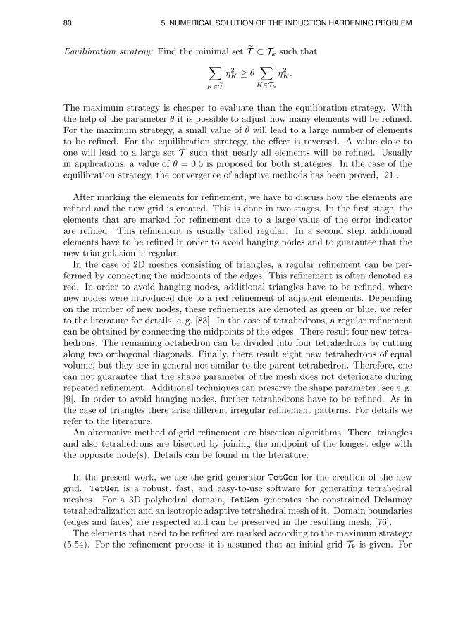
80 5. NUMERICAL SOLUTION OF THE INDUCTION HARDENING PROBLEM
Equilibration strategy: Find the minimal set T ⊂ Tk such that∑K∈T
η2K ≥ θ
∑K∈Tk
η2K .
The maximum strategy is cheaper to evaluate than the equilibration strategy. Withthe help of the parameter θ it is possible to adjust how many elements will be refined.For the maximum strategy, a small value of θ will lead to a large number of elementsto be refined. For the equilibration strategy, the effect is reversed. A value close toone will lead to a large set T such that nearly all elements will be refined. Usuallyin applications, a value of θ = 0.5 is proposed for both strategies. In the case of theequilibration strategy, the convergence of adaptive methods has been proved, [21].
After marking the elements for refinement, we have to discuss how the elements arerefined and the new grid is created. This is done in two stages. In the first stage, theelements that are marked for refinement due to a large value of the error indicatorare refined. This refinement is usually called regular. In a second step, additionalelements have to be refined in order to avoid hanging nodes and to guarantee that thenew triangulation is regular.
In the case of 2D meshes consisting of triangles, a regular refinement can be per-formed by connecting the midpoints of the edges. This refinement is often denoted asred. In order to avoid hanging nodes, additional triangles have to be refined, wherenew nodes were introduced due to a red refinement of adjacent elements. Dependingon the number of new nodes, these refinements are denoted as green or blue, we referto the literature for details, e. g. [83]. In the case of tetrahedrons, a regular refinementcan be obtained by connecting the midpoints of the edges. There result four new tetra-hedrons. The remaining octahedron can be divided into four tetrahedrons by cuttingalong two orthogonal diagonals. Finally, there result eight new tetrahedrons of equalvolume, but they are in general not similar to the parent tetrahedron. Therefore, onecan not guarantee that the shape parameter of the mesh does not deteriorate duringrepeated refinement. Additional techniques can preserve the shape parameter, see e. g.[9]. In order to avoid hanging nodes, further tetrahedrons have to be refined. As inthe case of triangles there arise different irregular refinement patterns. For details werefer to the literature.
An alternative method of grid refinement are bisection algorithms. There, trianglesand also tetrahedrons are bisected by joining the midpoint of the longest edge withthe opposite node(s). Details can be found in the literature.
In the present work, we use the grid generator TetGen for the creation of the newgrid. TetGen is a robust, fast, and easy-to-use software for generating tetrahedralmeshes. For a 3D polyhedral domain, TetGen generates the constrained Delaunaytetrahedralization and an isotropic adaptive tetrahedral mesh of it. Domain boundaries(edges and faces) are respected and can be preserved in the resulting mesh, [76].
The elements that need to be refined are marked according to the maximum strategy(5.54). For the refinement process it is assumed that an initial grid Tk is given. For

5.5. Averaging of the magnetic permeability 81
the creation of an initial grid with TetGen, it is possible to provide volume constraintsfor different regions of the geometry. For the refinement process, we can make use ofthis functionality. It is possible to prescribe volume constraints for each grid cell ofthe mesh Tk. Using e. g.
VK =1
8VK for K ∈ T ,
where T ⊂ Tk denotes the elements marked for refinement, VK the volume of the ele-ment K and VK the volume constraint for the cell K in the new grid Tk+1, correspondsto a regular refinement of the marked tetrahedrons.TetGen automatically creates a new grid Tk+1 by refining the old grid Tk, taking the
prescribed volume constraints VK for each element K ∈ Tk into account. The resultingmesh is regular, i. e. there are no hanging nodes, and the Delaunay property of themesh is satisfied. In order to preserve the Delaunay property, it might be possible thatadditional nodes are created or the mesh is smoothed. As a drawback of the smoothingone can not guarantee that the created meshes are hierarchic.
Since TetGen expects a volume constraint for the refinement process, we are notrestricted to regular refinements where e. g. the new volume is 1/8 of the old volume.It is also possible to construct the volume constraint for the new mesh in dependenceon the estimated error on each cell. A large estimated error would lead to morerefinements of the parent cell, while a small error might only require a bisection of theelement. We propose the following strategy to prescribe the volume constraint for themesh cell K ∈ Tk
VK = max
η0
ε
ηK, δ0
VK , (5.55)
where ε denotes the desired tolerance, δ0 some constant to bound the maximum reduc-tion of the new volume and η0 < 1 some constant to enforce a grid refinement if theratio ε/ηK ≈ 1. In this way, the reduction in the error might be accelerated and thenumber of iterations to obtain a prescribed accuracy might be reduced. A numericalexample, where a refinement using the maximum strategy is compared to the proposedstrategy (5.55), is presented in Section 6.1.
We use the strategy (5.55) together with the a posteriori error estimator introducedin Section 5.4.2 to create the adaptive grid for the simulation of the induction heatingproblem.
5.5. Averaging of the magnetic permeability
In ferromagnetic materials, the magnetic permeability is a nonlinear function. It de-pends on the temperature θ and the magnetic field H, cf. Section 3.4, i. e.
µ = µ(|H| , θ).
As a consequence, the vector potential equation is nonlinear and suitable solversare required. Using e. g. Newton’s method is computational costly. In Section 5.3 themethod of freezing coefficients is introduced. As a drawback, it might require quite

82 5. NUMERICAL SOLUTION OF THE INDUCTION HARDENING PROBLEM
small time steps to resolve the nonlinearity and to obtain an accurate solution for Ah.Furthermore, the curl-curl matrix Kµ has to be assembled in every time step of theMaxwell iteration. As a consequence, in every time step, the system matrices of thetime stepping scheme have to be updated and the matrix factorizations have to berecomputed, which is the most time consuming step.
Therefore, we introduce a method to linearize the vector potential equation. This isdone by an averaging procedure proposed in [18]. In induction heating problems, thefocus lies on the efficient computation of the Joule heat. The exact reproduction of themagnetic field is of minor importance as long as the Joule heat term J ·E = σ |∂tA|2is approximated with sufficient accuracy. Since only an averaged value of the Jouleheat enters the heat equation, it is assumed that it is sufficient to consider also atime averaged value of the permeability. In the following, we explain the algorithm tocompute the averaged permeability µ.
After decoupling the heat- and the vector potential equation as described in Section5.3 we consider the time interval (tk, tk+1) and assume that the temperature is givenat time tk. Furthermore, it is assumed that the vector potential equation has beensolved and a periodic solution for A is known on (tk, tk+1). It is assumed that thissolution has been obtained using a known averaged permeability µ(x). Then, theperiodic magnetic field is given by H = µ−1 curlA. The exact magnetic permeabilityis then a periodic function obtained from the nonlinear magnetization curve
µ(x, t) = µ(|H(x, t)| , θk(x)). (5.56)
Now, the new iterate of the averaged magnetic permeability µ(x) is obtained bycomputing the mean value of µ(x, t) over one period in the following way
1
µ(x)=
ω
2π
2πω∫
0
1
µ(x, t)dt. (5.57)
Using the inverse of µ for the averaging procedure is proposed in [18]. The authorsinvestigate different averaging techniques and consider an averaging of µ2, µ, µ−1 andµ−2. By numerical tests, the harmonic mean given in (5.57) performed best.
The permeability µ(x) is independent of A, it only depends on the space coordinatex and has to be computed in every point of the domain. It was assumed that a solutionof A is known on the actual time interval (tk, tk+1). Of course, A is only available forprevious time steps such that the averaged permeability µ has to be computed by afixed point iteration, starting e. g. with µ = µ0. Numerical tests have shown that theaveraging of the permeability converges typically within two to three iterations.
It is the advantage of the averaged permeability that µ is constant on the interval(tk, tk+1). The vector potential equation is linear and we can keep the matrix Kµ forthe whole interval (tk, tk+1), there is no need to reassemble and, more important, torecompute the matrix factorization. In this case, the time iteration of the vector poten-tial equation can be computed effectively using e. g. the PCG method in combinationwith PARDISO, cf. Section 5.3.6.

5.6. The complete algorithm to solve the induction hardening problem 83
Compared to the literature, a linearization of µ is a common approach. A similarapproach as described above is used in [48]. The technique is also used in actual publi-cations related to induction hardening, [36, 72]. A fictive linear material with a fictivepermeability µf is introduced. By an iterative procedure, the fictive permeability iscomputed by energetic considerations. This approach can be easily implemented whenconsidering Maxwell’s equations in the frequency domain, since it only involves themagnetic energy H ·B. Ostrowski [60] introduces an effective permeability µeff byaveraging the nonlinear permeability over one period similar as described above.
5.6. The complete algorithm to solve the induction hardeningproblem
The solution of the system of partial and ordinary differential equations (5.9) is ob-tained using the software package pdelib, which is developed and maintained at WIASBerlin. The pdelib is a modular software package based on C/C++ to solve partialdifferential equations by the finite element or finite volume method [61].
In pdelib, hierarchical finite elements for H1 are available. In order to solve thevector potential equation, edge based elements of Nedelec type as described in Section5.2.4 are used. These were implemented in pdelib. The complete algorithm to sim-ulate the inductive heating for gears consisting of the methods described in Sections5.1 to 5.5 is summarized in the following.
1. Initialization.
The first step consists in the definition of the scenario, i. e. the definition of theheating time T , the specification of the MF and HF frequencies fmf and fhf andthe relative power pmf and phf corresponding MF and HF, cf. equation (3.25).Furthermore, one has to define an error tolerance ε for the error estimator to createan adaptive grid. Then, the geometry description is read from a file and a coarseinitial grid is created using TetGen.
2. Adaptive grid generation.
Setting the initial magnetic permeability to µ = µ0 the vector potential equation issolved for some time steps (one fourth of a period) using edge based finite elementsfor the discretization in space and a Crank-Nicolson scheme in time on the coarsegrid. The error estimator η, equation (5.53), is evaluated on each element and foreach time step. The estimated local errors are summed up for the time steps to getan indicator, which mesh cells need to be refined. A refined grid is created usingTetGen together with (5.55) until maxK∈T η ≤ ε.
3. Time iteration of the magnetic vector potential.
We set the time step count to k = 0 and tk = 0. Since in the case of multifrequencyinduction hardening the high frequency might be by a factor of 20 higher than themedium frequency (typically fmf = 10 kHz and fhf = 200 kHz), it is recommendedto split the magnetic vector potential A into a MF and HF part
A = Amf +Ahf.

84 5. NUMERICAL SOLUTION OF THE INDUCTION HARDENING PROBLEM
With the use of the averaged magnetic permeability, cf. Section 5.5, the vectorpotential equation is linear such that Amf and Ahf are the solutions of
σ∂tAmf + curlµ−1 curlAmf = Jsrc,mf and
σ∂tAhf + curlµ−1 curlAhf = Jsrc,hf
where Jsrc = Jsrc,mf + Jsrc,hf and
Jsrc,mf = Imf pmf(t) cos(2πfmft)J0(x) and Jsrc,hf = Ihf phf(t) cos(2πfhft)J0(x).
We solve the equations above separately using a BDF-2 discretization in time, seeSection 5.3.1, in combination with the PCG method and PARDISO as precondi-tioner, Section 5.3.2, until we obtain a periodic solution for Amf and Ahf.
(a) Computation of the averaged magnetic permeability.
The update of the averaged magnetic permeability requires knowledge of thecomplete vector potential field A = Amf + Ahf. The vector potential A isdetermined from the periodic solutions forAmf andAhf by interpolation. Then,the averaging of µ is done according to Section 5.5. We iterate the computationof Amf, Ahf and µ until there is no significant change in µ.
(b) Computation of the averaged Joule heat.
Since the functions sin(2πkt) and cos(2πkt), k ∈ N, are orthogonal, there holdsfor the averaged Joule heat
|∂tA|2 = |∂tAmf|2 + |∂tAhf|2 ,
provided that the high frequency is an integer multiple of the medium frequency:ωhf = nωmf with n ∈ N. As a consequence, the averaging of the Joule heat canbe done separately for the medium and high frequency parts as described inSection 5.3.4. The overall Joule heat entering the right hand side is obtainedby summing up both contributions.
4. Time iteration of the heat equation.
With the heat source given by the averaged Joule heat, the next step is the com-putation of the temperature and the volume fraction of austenite for the new timestep tk+1 by solving equations (5.42) and (5.41) as described in Section 5.3.4.
5. Finally, set k = k + 1 and iterate steps 3. and 4. until tk ≥ T .
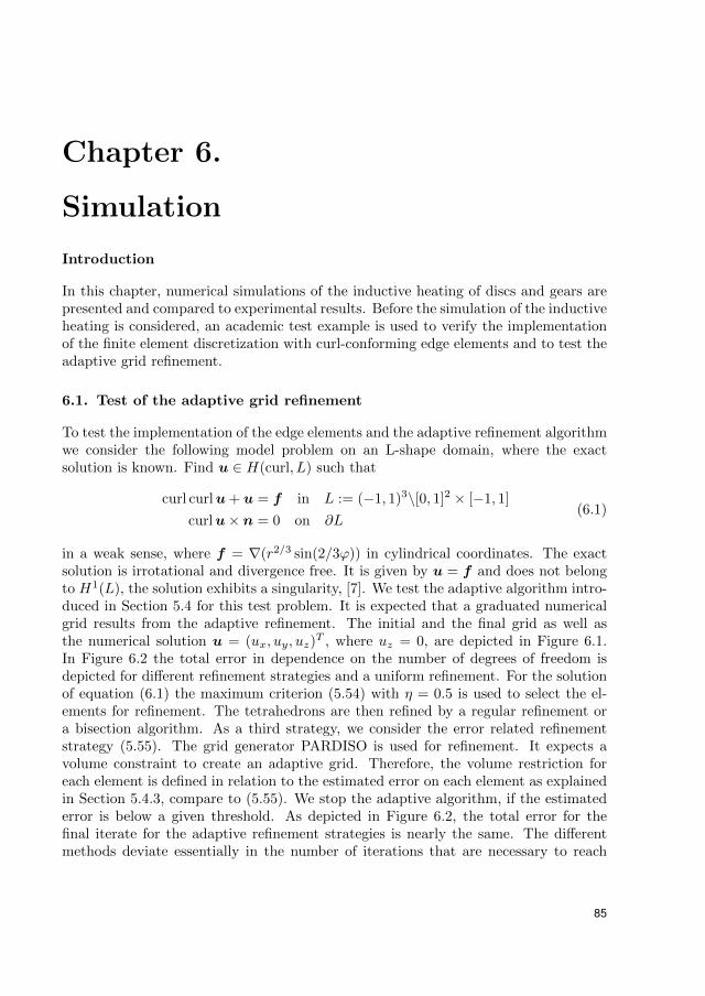
Chapter 6.
Simulation
Introduction
In this chapter, numerical simulations of the inductive heating of discs and gears arepresented and compared to experimental results. Before the simulation of the inductiveheating is considered, an academic test example is used to verify the implementationof the finite element discretization with curl-conforming edge elements and to test theadaptive grid refinement.
6.1. Test of the adaptive grid refinement
To test the implementation of the edge elements and the adaptive refinement algorithmwe consider the following model problem on an L-shape domain, where the exactsolution is known. Find u ∈ H(curl, L) such that
curl curlu+ u = f in L := (−1, 1)3\[0, 1]2 × [−1, 1]
curlu× n = 0 on ∂L(6.1)
in a weak sense, where f = ∇(r2/3 sin(2/3ϕ)) in cylindrical coordinates. The exactsolution is irrotational and divergence free. It is given by u = f and does not belongto H1(L), the solution exhibits a singularity, [7]. We test the adaptive algorithm intro-duced in Section 5.4 for this test problem. It is expected that a graduated numericalgrid results from the adaptive refinement. The initial and the final grid as well asthe numerical solution u = (ux, uy, uz)
T , where uz = 0, are depicted in Figure 6.1.In Figure 6.2 the total error in dependence on the number of degrees of freedom isdepicted for different refinement strategies and a uniform refinement. For the solutionof equation (6.1) the maximum criterion (5.54) with η = 0.5 is used to select the el-ements for refinement. The tetrahedrons are then refined by a regular refinement ora bisection algorithm. As a third strategy, we consider the error related refinementstrategy (5.55). The grid generator PARDISO is used for refinement. It expects avolume constraint to create an adaptive grid. Therefore, the volume restriction foreach element is defined in relation to the estimated error on each element as explainedin Section 5.4.3, compare to (5.55). We stop the adaptive algorithm, if the estimatederror is below a given threshold. As depicted in Figure 6.2, the total error for thefinal iterate for the adaptive refinement strategies is nearly the same. The differentmethods deviate essentially in the number of iterations that are necessary to reach
85

86 6. SIMULATION
(a) coarse grid (b) fine grid (c) ux (d) uy
Figure 6.1.: Coarsest and finest grid and numerical solution u = (ux, uy, uz) for prob-lem (6.1)
102 103 104 105
10−2
10−1
degrees of freedom
erro
r
error-adaptedregular ref., η = 0.5bisection, η = 0.5
uniform refinement
Figure 6.2.: Comparison of different adaptive grid generation strategies

6.2. Numerical simulations for discs 87
the prescribed error tolerance. While the adaptive methods using the maximum cri-terion require 11 (regular refinement) or 14 (bisection) iterations, the proposed errorrelated strategy reaches the prescribed error tolerance after 5 cycles and the numberof degrees of freedom for the final iterate is nearly the same as for the other strategies.Due to the design of the error based refinement strategy the relation between degreesof freedom and total error is not optimal for the intermediate iterates. For these it iscomparable to a uniform refinement and the other strategies show better performance.Nevertheless, we prefer the error related refinement strategy since the solution of thevector potential equation is the most time consuming step during the adaptive gridgeneration process.
6.2. Numerical simulations for discs
6.2.1. Numerical simulations
As the next step, we consider numerical simulations of induction heating for discs andperform an experimental verification. In order to account for the different couplingdistances that occur in the case of gears, discs with three different radii are considered,which correspond to the addendum circle (47.7 mm), the pitch circle (42 mm) and theroot circle (38.7 mm) of the reference gear used in Section 6.3. This results in differentcoupling distances. The width of the discs is taken as 8 mm.
The parameters for the simulation are shown in Table 6.1, which result in nine dif-ferent cases. To allow for an experimental verification, the parameters are matched toexperiments carried out by IWT Bremen. This is necessary, since e. g. the frequencycan not be adjusted freely. The multifrequency converter operates at the resonantfrequency of the oscillating circuit, consisting of the inductor coil, the converter, con-nection cables and the necessary filters and adaptation capacitors to compensate thereactive power. The experimental setup is described in detail in Section 6.2.2.
Parameter Variants
Diameter 47.7 mm 42 mm 38.7 mm
(addendum circle) (pitch circle) (root circle)
Coupling distance 1.15 mm 4 mm 5.65 mm
Induction heating HF MF (MF+HF)
Frequency 200 kHz 12 kHz 12 kHz + 200 kHz
Power in % 50 % 63 % 46 % (MF) + 35 % (HF)
Table 6.1.: Parameter variants for the experimental verification of discs
For the numerical simulations of the disc specimen it is possible to reduce the ge-ometric complexity by exploiting the symmetry of the workpiece. It is not necessaryto simulate the complete disc. The cross section of a horizontal cut serves as a sym-metry plane. In addition, due to angular symmetry, it is possible to consider only a

88 6. SIMULATION
segment of the disc 1. The disc geometry is depicted in Figure 6.3. The reduced com-putational domain is indicated in red, where for the sake of presentation the domaincorresponding to the surrounding air is blanked out.
Figure 6.3.: Computational domain using symmetry conditions (exemplary for thedisc)
It is necessary to define boundary conditions on the cutting planes for the reducedgeometry. For this, we denote the horizontal cross section by ΓH . The vertical cuts aredenoted by ΓV . Since the source current Jsrc is defined only in angular direction, theradial and the z-component of the magnetic vector potential A are zero on the verticalcutting planes. Therefore, the tangential components of A vanish on ΓV , A× n = 0.
The magnetic induction B is perpendicular to A. As a consequence, the magneticfield H has only non-vanishing normal components on the horizontal cutting planeΓH . All together there holds
A× n = 0 on ΓV and µ−1 curlA× n = 0 on ΓH .
These boundary conditions arising from symmetry conditions correspond to the con-ditions (PEC) and (PMC) introduced in (3.12).
For the reduced disc geometry, simulations of the heating procedure are carried out.The heating time is set to 1.0 s. Since in the experiments a temperature measurementby pyrometer is not possible during the heating process but only immediately afterswitching off the current, the effect of self-cooling with the source term set to zero, i. e.Jsrc = 0, is taken into account and the simulation time is extended up to 1.2 s.
In the following we present detailed simulation results for the disc with diameter d =47.7 mm. The obtained results are discussed in Section 6.2.3. The grids that are usedfor the finite element simulations for the case of medium, high and multi-frequency aredepicted in Figure 6.4. The grids are generated adaptively by the algorithm describedin Section 5.4. The grid is adapted to the frequency dependent penetration depth of
1Due to angular symmetry it is possible to consider the setting in 2D. We are interested in theperformance and the calibration of our 3D algorithm and consider a 3D geometry. The angle hasbeen chosen as half the size of a tooth as for the gear experiments.

6.2. Numerical simulations for discs 89
(a) MF (b) HF (c) MF+HF
Figure 6.4.: Comparison of the adaptively generated grids
the eddy currents. In the case of high frequency, the grid is very fine in a small surfacelayer of the workpiece, while in the case of medium frequency the elements are refinedalso within the workpiece. In the case of multifrequency, the MF part dominates suchthat the grid is quite similar to the medium frequency case, cf. Fig. 6.4.
Disc with diameter 47.7 mm, MF
The simulation results for the disc heated with medium frequency are depicted in Fig-ure 6.5. The temperature profile and the corresponding phase fraction of austeniteare depicted for different time snapshots. The maximum temperature is reached after1.0 s, Fig. 6.5 (c). Since the experimental measurement of the temperature by a py-rometer is only possible with a delay, the simulation is continued. The temperaturereduces due to heat diffusion. The final temperature after 1.2 s and the correspondingaustenitic fraction are depicted in Fig. 6.5 (d).
Disc with diameter 47.7 mm, HF
In Figure 6.6, the results using high frequency power are shown. As above, the tem-perature profile and the austenite fraction for different time snapshots are presented.Compared to the case of medium frequency, the profile of the austenite is concave whilein the case of MF it is convex. This is due to the fact that the highest temperature isattained at the upper corner of the disc, Fig. 6.6 (b).
Disc with diameter 47.7 mm, MF+HF
Finally, the temperature profiles and the corresponding austenite fraction for the caseof simultaneous applied medium and high frequency power is shown in Figure 6.7.The most significant difference to the single frequency case is the nearly homogeneousaustenitic profile, while in the case of MF, the profile is convex and in the case of HFa concave profile results.

90 6. SIMULATION
(a) t = 0.5 s (b) t = 0.7 s (c) t = 1.0 s (d) t = 1.2 s
Figure 6.5.: Temperature θ and phase fraction of austenite z for the disc with diameterd = 47.7 mm, MF: f = 12 kHz
(a) t = 0.7 s (b) t = 1.0 s (c) t = 1.2 s
Figure 6.6.: Temperature θ and phase fraction of austenite z for the disc with diameterd = 47.7 mm, HF: f = 204 kHz

6.2. Numerical simulations for discs 91
(a) t = 0.7 s (b) t = 1.0 s (c) t = 1.2 s
Figure 6.7.: Temperature θ and phase fraction of austenite z for the disc with diameterd = 47.7 mm, MF+HF: f = 12 kHz + 204 kHz.
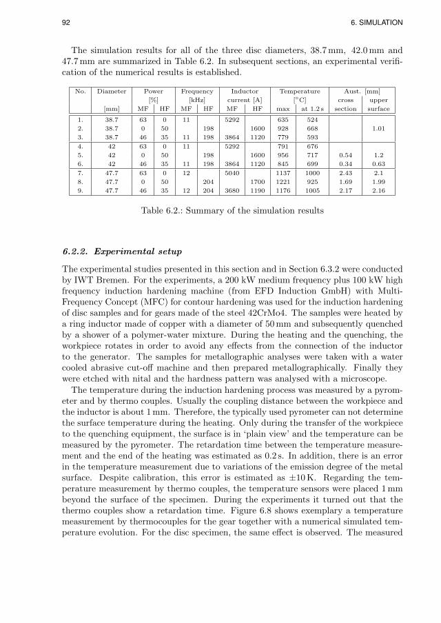
92 6. SIMULATION
The simulation results for all of the three disc diameters, 38.7 mm, 42.0 mm and47.7 mm are summarized in Table 6.2. In subsequent sections, an experimental verifi-cation of the numerical results is established.
No. Diameter Power Frequency Inductor Temperature Aust. [mm]
[%] [kHz] current [A] [C] cross upper
[mm] MF HF MF HF MF HF max at 1.2 s section surface
1. 38.7 63 0 11 5292 635 524
2. 38.7 0 50 198 1600 928 668 1.01
3. 38.7 46 35 11 198 3864 1120 779 593
4. 42 63 0 11 5292 791 676
5. 42 0 50 198 1600 956 717 0.54 1.2
6. 42 46 35 11 198 3864 1120 845 699 0.34 0.63
7. 47.7 63 0 12 5040 1137 1000 2.43 2.1
8. 47.7 0 50 204 1700 1221 925 1.69 1.99
9. 47.7 46 35 12 204 3680 1190 1176 1005 2.17 2.16
Table 6.2.: Summary of the simulation results
6.2.2. Experimental setup
The experimental studies presented in this section and in Section 6.3.2 were conductedby IWT Bremen. For the experiments, a 200 kW medium frequency plus 100 kW highfrequency induction hardening machine (from EFD Induction GmbH) with Multi-Frequency Concept (MFC) for contour hardening was used for the induction hardeningof disc samples and for gears made of the steel 42CrMo4. The samples were heated bya ring inductor made of copper with a diameter of 50 mm and subsequently quenchedby a shower of a polymer-water mixture. During the heating and the quenching, theworkpiece rotates in order to avoid any effects from the connection of the inductorto the generator. The samples for metallographic analyses were taken with a watercooled abrasive cut-off machine and then prepared metallographically. Finally theywere etched with nital and the hardness pattern was analysed with a microscope.
The temperature during the induction hardening process was measured by a pyrom-eter and by thermo couples. Usually the coupling distance between the workpiece andthe inductor is about 1 mm. Therefore, the typically used pyrometer can not determinethe surface temperature during the heating. Only during the transfer of the workpieceto the quenching equipment, the surface is in ‘plain view’ and the temperature can bemeasured by the pyrometer. The retardation time between the temperature measure-ment and the end of the heating was estimated as 0.2 s. In addition, there is an errorin the temperature measurement due to variations of the emission degree of the metalsurface. Despite calibration, this error is estimated as ±10 K. Regarding the tem-perature measurement by thermo couples, the temperature sensors were placed 1 mmbeyond the surface of the specimen. During the experiments it turned out that thethermo couples show a retardation time. Figure 6.8 shows exemplary a temperaturemeasurement by thermocouples for the gear together with a numerical simulated tem-perature evolution. For the disc specimen, the same effect is observed. The measured

6.2. Numerical simulations for discs 93
temperature curve is shifted by some tenth of a second compared to the simulation.Especially the fact, that the temperature still rises significantly after the heating poweris turned off can not be explained by heat conduction effects alone. This is an indica-tion that the delay results from a thermal inertia of the thermo couple. The effect isstronger in the tip of the tooth, where higher heating rates are achieved. Since thereis this delay, we do not use the thermo couple measurements for verification purpose.
0
20
40
60
80
pow
er[%
]
1.5 2 2.5 3 3.5 4 4.5 50
200
400
600
800
time [s]
tem
per
ature
[C
]
measured temp. (tip)
measured temp. (root)
simulated temp. (tip)
simulated temp. (root)
Figure 6.8.: Exemplary evolution of the simulated and the measured temperature bythermo-elements positioned 1 mm below surface; the grey curves indicatethe MF and HF power
In addition to the temperature, measurements of the hardness in the surface areawere performed. From these values, the hardening depth can be estimated as thedistance, where the hardness drops below some threshold. It is directly related to theamount of martensite that has been formed during the hardening process.
In the simulation of the inductive heating, the austenite faction z is computed. Inorder to compare simulation and experiment, we have to relate this information to themeasured hardness or the martensitic profile. Since the subsequent quenching pro-cedure is not considered in this work, it is assumed that during the quenching, theaustenite transforms completely into martensite. This fact is confirmed by experimen-tal observations. The hardening depth obtained from the experiment is then comparedto the penetration depth of the austenite phase z.
For the numerical simulation it is necessary to define the source current density Jsrc
in the inductor. Therefore, knowledge of the inductor current is necessary to comparesimulation and experiment. A direct measurement of the current in the induction coilis not possible. Typically in technical applications, the induction heating process ispower controlled. The power of the medium and high frequency is given as relativevalue in percent, related to the maximum possible value of the hardening machine for agiven frequency. Nevertheless, the current is the crucial quantity for the generation of
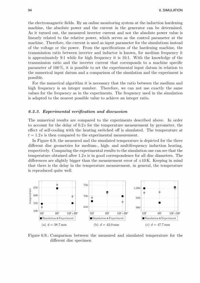
94 6. SIMULATION
the electromagnetic fields. By an online monitoring system at the induction hardeningmachine, the absolute power and the current in the generator can be determined.As it turned out, the measured inverter current and not the absolute power value islinearly related to the relative power, which serves as the control parameter at themachine. Therefore, the current is used as input parameter for the simulations insteadof the voltage or the power. From the specifications of the hardening machine, thetransmission ratio between inverter and inductor is known, for medium frequency itis approximately 9:1 while for high frequency it is 10:1. With the knowledge of thetransmission ratio and the inverter current that corresponds to a machine specificparameter of 100 %, it is possible to set the experimental input datum in relation tothe numerical input datum and a comparison of the simulation and the experiment ispossible.
For the numerical algorithm it is necessary that the ratio between the medium andhigh frequency is an integer number. Therefore, we can not use exactly the samevalues for the frequency as in the experiments. The frequency used in the simulationis adapted to the nearest possible value to achieve an integer ratio.
6.2.3. Experimental verification and discussion
The numerical results are compared to the experiments described above. In orderto account for the delay of 0.2 s for the temperature measurement by pyrometer, theeffect of self-cooling with the heating switched off is simulated. The temperature att = 1.2 s is then compared to the experimental measurement.
In Figure 6.9, the measured and the simulated temperature is depicted for the threedifferent disc geometries for medium-, high- and multifrequency induction heating,respectively. Comparing the experimental results to the simulation one can see that thetemperature obtained after 1.2 s is in good correspondence for all disc diameters. Thedifferences are slightly bigger than the measurement error of ±10 K. Keeping in mindthat there is the delay in the temperature measurement, in general, the temperatureis reproduced quite well.
MF HF MF+HF500
550
600
650
tem
per
ature
Simulation Experiment
(a) d = 38.7 mm
MF HF MF+HF
650
700
750
Simulation Experiment
(b) d = 42.0 mm
MF HF MF+HF
900
950
1,000
Simulation Experiment
(c) d = 47.7 mm
Figure 6.9.: Comparison between the measured and simulated temperature for thedifferent disc specimen

6.2. Numerical simulations for discs 95
One has to mention that the focus was not to fit the simulated temperature to theexperimental result. It was the aim to use an input datum that can be directly relatedto machine parameters. With the knowledge of the transformation ratio between theinverter and the inductor we obtain an estimate of the inductor current, which is usedas a source term in the simulation, compare Section 3.1.4.
The obtained hardening depths for the experiment and the simulation are opposedin Table 6.3. In the case of the largest coupling distance, the maximum temperatureslie below the austenitization temperature such that no phase transition occurred.
No. Frequency Diameter Aust. [mm] Exp. hardening depth [mm]
[mm] cross section norm. Q&T low t. Q&T high t.
1. MF 38.7
2. HF 38.7 0.16 0.49
3. MF+HF 38.7
4. MF 42 0.59 0.59 1.06
5. HF 42 0.54 0.64 0.6 0.87
6. MF+HF 42 0.34 0.27 0.16 0.69
7. MF 47.7 2.43 2.61 2.6 2.78
8. HF 47.7 1.69 1.95 1.94 2.16
9. MF+HF 47.7 2.17 2.35 2.11 2.56
Table 6.3.: Comparison between simulated and experimental hardening depth
For the heating of the disc with diameter d = 42 mm a phase transition occurs.In the case of using pure HF and simultaneously applied MF+HF, No. 5 and 6, thesimulated hardening depths lie in the range of the experimentally observed ones. In thecase of heating with pure MF, No. 4, the austenitization temperature is not reachedin the simulation while in the experiment, a phase transition occurs and a hardeningdepth of 0.59 mm is obtained. Opposed to that, the simulated temperature after 1.2 slies in a comparable range and is only 20 K below the experimental result.
In general, the experimental results could be reproduced quite well. Especially forthe largest disc with d = 47.7 mm, which corresponds to a realistic coupling distancein induction heating of cylindrical shaped workpieces such as shafts, there is a goodcorrespondence between experimental and computational result. This holds true forthe temperature as well as the hardening depth.
A further indication of the good correspondence between experiment and simula-tion represents the lateral profile of the austenitic phase fraction. In Figure 6.10 thecomputed profile is compared to micrographs of a lateral cut through the disc withdiameter d = 47.7 mm for pure MF, HF and the case of multifrequency. In the caseof medium frequency, a convex profile results, where the penetration depth is higherin the centre of the disc. For HF the profile is concave, while in the case of the si-multaneous applied medium and high frequency a nearly homogeneous profile couldbe observed. In the experiments, three different initial states for the microstructurewere considered, which are a normalized state and two different states quenched andtempered (Q&T). The dependence on the initial microstructure can not be resolveddirectly by the numerical simulation. The austenitization behaviour is recaptured bythe evolution equation for the phase fraction of austenite z in terms of equation (3.26).
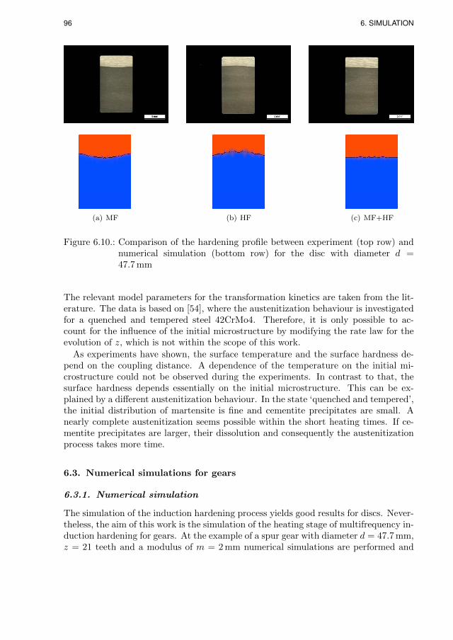
96 6. SIMULATION
(a) MF (b) HF (c) MF+HF
Figure 6.10.: Comparison of the hardening profile between experiment (top row) andnumerical simulation (bottom row) for the disc with diameter d =47.7 mm
The relevant model parameters for the transformation kinetics are taken from the lit-erature. The data is based on [54], where the austenitization behaviour is investigatedfor a quenched and tempered steel 42CrMo4. Therefore, it is only possible to ac-count for the influence of the initial microstructure by modifying the rate law for theevolution of z, which is not within the scope of this work.
As experiments have shown, the surface temperature and the surface hardness de-pend on the coupling distance. A dependence of the temperature on the initial mi-crostructure could not be observed during the experiments. In contrast to that, thesurface hardness depends essentially on the initial microstructure. This can be ex-plained by a different austenitization behaviour. In the state ‘quenched and tempered’,the initial distribution of martensite is fine and cementite precipitates are small. Anearly complete austenitization seems possible within the short heating times. If ce-mentite precipitates are larger, their dissolution and consequently the austenitizationprocess takes more time.
6.3. Numerical simulations for gears
6.3.1. Numerical simulation
The simulation of the induction hardening process yields good results for discs. Never-theless, the aim of this work is the simulation of the heating stage of multifrequency in-duction hardening for gears. At the example of a spur gear with diameter d = 47.7 mm,z = 21 teeth and a modulus of m = 2 mm numerical simulations are performed and
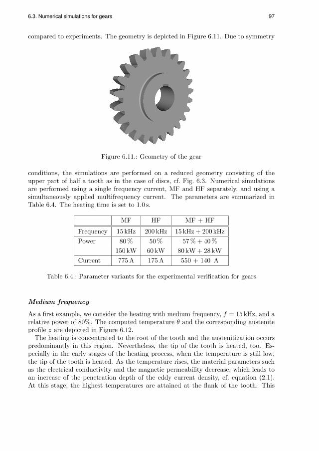
6.3. Numerical simulations for gears 97
compared to experiments. The geometry is depicted in Figure 6.11. Due to symmetry
Figure 6.11.: Geometry of the gear
conditions, the simulations are performed on a reduced geometry consisting of theupper part of half a tooth as in the case of discs, cf. Fig. 6.3. Numerical simulationsare performed using a single frequency current, MF and HF separately, and using asimultaneously applied multifrequency current. The parameters are summarized inTable 6.4. The heating time is set to 1.0 s.
MF HF MF + HF
Frequency 15 kHz 200 kHz 15 kHz + 200 kHz
Power 80 % 50 % 57 % + 40 %
150 kW 60 kW 80 kW + 28 kW
Current 775 A 175 A 550 + 140 A
Table 6.4.: Parameter variants for the experimental verification for gears
Medium frequency
As a first example, we consider the heating with medium frequency, f = 15 kHz, and arelative power of 80%. The computed temperature θ and the corresponding austeniteprofile z are depicted in Figure 6.12.
The heating is concentrated to the root of the tooth and the austenitization occurspredominantly in this region. Nevertheless, the tip of the tooth is heated, too. Es-pecially in the early stages of the heating process, when the temperature is still low,the tip of the tooth is heated. As the temperature rises, the material parameters suchas the electrical conductivity and the magnetic permeability decrease, which leads toan increase of the penetration depth of the eddy current density, cf. equation (2.1).At this stage, the highest temperatures are attained at the flank of the tooth. This

98 6. SIMULATION
↑symmetry plane
(a) t = 0.6 s (b) t = 0.8 s (c) t = 1.0 s
Figure 6.12.: Temperature und austenitic fraction, MF: f = 15 kHz
can be seen in Figure 6.12 (a). With further increase of the temperature, the heatingpredominantly occurs in the root of the tooth. After a heating time of 1.0 s, the rootof the tooth is nearly through hardened.
To illustrate the effect of the Joule heating and the changing penetration depth, the
averaged power density per unit volume of the eddy currents, Q = 1/T∫ T
0σ |∂tA|2 dt,
is depicted in Figure 6.13.
In the beginning, the heat power concentrates in the surface region of the flank ofthe tooth. But already at the early stage, the maximum power is attained at the rootof the tooth. Nevertheless, the maximum temperature is attained at the tip or theflank of the tooth, cf. Fig. 6.12. This can be explained by the fact that heat conductionin the root of the tooth is extremely high. Most of the heat is conducted into the coreof the gear, while due to the small volume of the tooth, the heat accumulates at thetooth tip.
With rising temperature, the penetration depth of the eddy currents rises. At theend of the heating procedure, the heat power concentrates completely to the root ofthe tooth, Fig. 6.13 (c). Comparing the beginning and the end of the heating, themagnitude of the heat power reduces significantly. This can be explained by the fact,that above the Curie point, the material loses its ferromagnetic properties and thegenerated heat reduces drastically.
In Figure 6.17 (a), the temperature evolution at the tip and the root of the tooth

6.3. Numerical simulations for gears 99
(a) t = 0.0 s (b) t = 0.5 s (c) t = 1.0 s
Figure 6.13.: Magnitude of the Joule heat using MF; the skin depth increases withrising temperature
is depicted. This figure illustrates again the afore mentioned process. In the earlystage of heating, the temperature increase at the tip of the tooth is higher, though themaximum of the heat power is attained at the root. The reason for this is the heatconduction. During the evolution, the temperature at the root of the tooth rises abovethe austenitization temperature and the phase transition occurs.
High frequency
As next example, we consider the inductive heating of the gear with high frequency,f = 195 kHz, and a relative power of 50%. The results are shown in Figure 6.14.
In this case, the heating concentrates to the tip of the tooth. Nevertheless, as thetemperature rises, the skin depth increases and also the root of the tooth is affectedby the heating. After a heating time of 1.0 s, the tooth is completely transformedto austenite due to the rising skin depth and heat conduction effects. In Figure 6.15the averaged heat power density is depicted. As in the case of MF, the power isconcentrated on the complete flank of the tooth. Compared to MF, Fig. 6.13, theskin depth is reduced. With rising temperature, the penetration depth rises and themaximum of the heat power concentrates at the root of the tooth, Fig. 6.15 (b). But incontrast to MF, there is still heat generation at the tooth tip. Due to heat conductionto the core of the gear and the already mentioned accumulation of heat in the toothtip, the maximum of the temperature is attained at the tip of the tooth despite thefact that the heat input is larger at the root at later stages of heating, Fig. 6.15 (c).This can also be seen in the temporal temperature evolution in the tip and the rootof the tooth, depicted in Figure 6.17 (b) for the case of HF.
Multifrequency concept
The computations using the multifrequency approach are shown in Figure 6.16. Theheating occurs simultaneously at the tip, the flank and the root of the tooth. The

100 6. SIMULATION
↑symmetry plane
(a) t = 0.5 s (b) t = 0.8 s (c) t = 1.0 s
Figure 6.14.: Temperature und austenitic phase fraction, HF: f = 195 kHz
(a) t = 0.0 s (b) t = 0.5 s (c) t = 1.0 s
Figure 6.15.: Magnitude of the Joule heat for induction heating using HF

6.3. Numerical simulations for gears 101
↑symmetry plane
(a) t = 0.6 s (b) t = 0.8 s (c) t = 1.0 s
Figure 6.16.: Temperature und austenite fraction, MF+HF: f = 15 kHz + 195 kHz
austenitic profile after a heating time of 1.0 s is shown in Figure 6.16 (c). A contourhardening of the gear with the chosen parameters can not be achieved. For a contourhardening, a heating time of 1.0 s might already be too long. Heat conduction effectslead to a nearly complete austenitization of the whole tooth. In order to avoid theseeffects, shorter heating times are necessary, which demand the use of higher powerinput.
In Figure 6.17 the temporal evolution of the temperature in the root and the tipof the tooth for the three different heating strategies is shown. This illustrates theheating procedure described in this section once again. For medium frequency, firstthe tooth tip is heated. Above the Curie temperature, the heat generation in theroot of the tooth dominates such that the temperature rises above the austenitizationtemperature only in the root of the tooth. In Figure 6.17 (a) we can also observe theoccurrence of the phase transition. Due to the latent heat that is consumed duringthe formation of austenite, there is a reduction in the heating rate (approx. at 0.75 sand a temperature of 820 C, cf. also Fig. 2.4). In the case of high frequency, Fig. 6.17(b), the temperature reaches the austenitization temperature only in the tooth tip.Due to the effect of the latent heat, a decrease of the temperature in the tip of thetooth occurs at approx. 0.25 s. Since above the Curie temperature, the heat powerconcentrates in the root of the tooth, the decrease of the heating rate in the tip isstronger than for the medium frequency case. For the multi frequency approach,
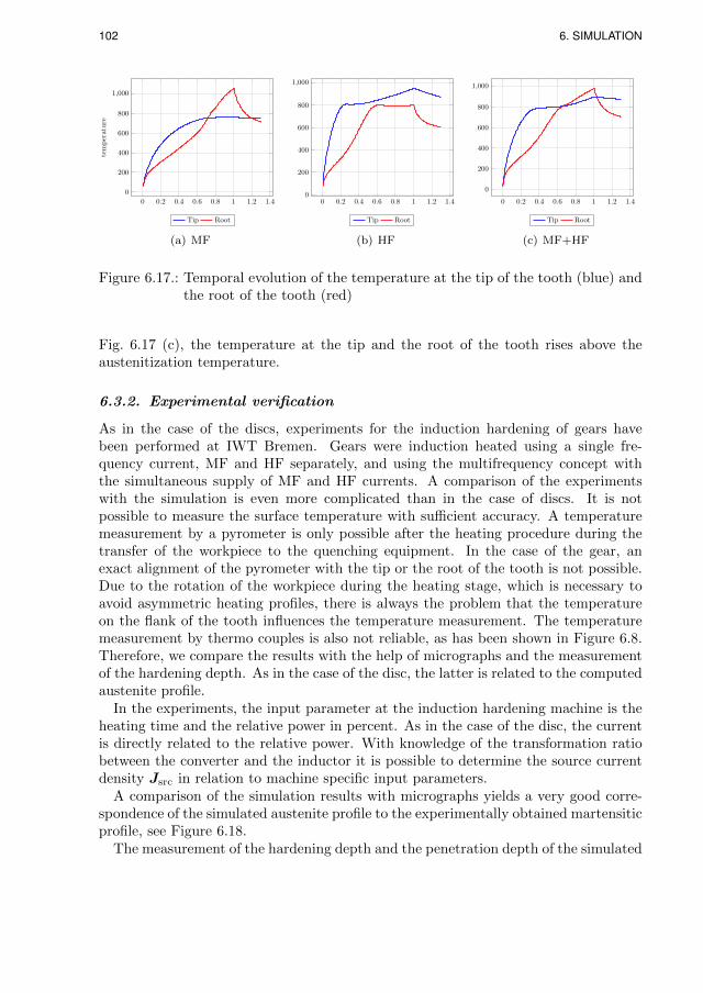
102 6. SIMULATION
0 0.2 0.4 0.6 0.8 1 1.2 1.4
0
200
400
600
800
1,000
tem
per
ature
Tip Root
(a) MF
0 0.2 0.4 0.6 0.8 1 1.2 1.40
200
400
600
800
1,000
Tip Root
(b) HF
0 0.2 0.4 0.6 0.8 1 1.2 1.4
0
200
400
600
800
1,000
Tip Root
(c) MF+HF
Figure 6.17.: Temporal evolution of the temperature at the tip of the tooth (blue) andthe root of the tooth (red)
Fig. 6.17 (c), the temperature at the tip and the root of the tooth rises above theaustenitization temperature.
6.3.2. Experimental verification
As in the case of the discs, experiments for the induction hardening of gears havebeen performed at IWT Bremen. Gears were induction heated using a single fre-quency current, MF and HF separately, and using the multifrequency concept withthe simultaneous supply of MF and HF currents. A comparison of the experimentswith the simulation is even more complicated than in the case of discs. It is notpossible to measure the surface temperature with sufficient accuracy. A temperaturemeasurement by a pyrometer is only possible after the heating procedure during thetransfer of the workpiece to the quenching equipment. In the case of the gear, anexact alignment of the pyrometer with the tip or the root of the tooth is not possible.Due to the rotation of the workpiece during the heating stage, which is necessary toavoid asymmetric heating profiles, there is always the problem that the temperatureon the flank of the tooth influences the temperature measurement. The temperaturemeasurement by thermo couples is also not reliable, as has been shown in Figure 6.8.Therefore, we compare the results with the help of micrographs and the measurementof the hardening depth. As in the case of the disc, the latter is related to the computedaustenite profile.
In the experiments, the input parameter at the induction hardening machine is theheating time and the relative power in percent. As in the case of the disc, the currentis directly related to the relative power. With knowledge of the transformation ratiobetween the converter and the inductor it is possible to determine the source currentdensity Jsrc in relation to machine specific input parameters.
A comparison of the simulation results with micrographs yields a very good corre-spondence of the simulated austenite profile to the experimentally obtained martensiticprofile, see Figure 6.18.
The measurement of the hardening depth and the penetration depth of the simulated

6.3. Numerical simulations for gears 103
(a) MF (b) HF (c) MF+HF
Figure 6.18.: Comparison of the hardening profile between experiment (top row) andnumerical simulation (bottom row)
austenite fraction are opposed in Table 6.5. Again, the simulation results reflect theexperiments very well.
No. Power Frequency Sim. austenitization Exp. hardening
[kW] [kHz] depth [mm] depth [mm]
MF HF MF HF tip root tip root
1. 150 (80%) 15 – 0.752 – 0.52
2. 60 (50%) 195 3.35 0.24 3.77 0.24
3. 80 (57%) 28 (40%) 15 195 3.01 0.24 3.37 0.24
Table 6.5.: Comparison of the hardening depth between simulation and experiment
The computations shown in Fig. 6.18 (c) using the multifrequency approach did notlead to a satisfactory contour hardening. For a heating time of 1.0 s, the influence ofheat conduction effects becomes significant. Therefore, in order to achieve a contourhardening of the gear, shorter heating times are necessary. Further experiments werecarried out and are presented in the following section.
2Penetration depth after 0.9 s. Due to an overestimation of the MF power, see Section 6.3.4, theheating time is reduced for a comparison between simulation and experiment.

104 6. SIMULATION
6.3.3. Contour hardening of gears in an industrial setting
In order to obtain a contour hardened gear, shorter heating times in connection withhigh heating rates are necessary. The experiments related to the following simulationswere done on a machine with higher power output at EFD Induction, Freiburg. Theobjective was the contour hardening of the gear depicted in Figure 6.11. In orderto determine the correct machine parameters, experiments with subsequent metallo-graphical analysis of the hardening profile were carried out by trial and error. Afterseveral experiments a set of parameters was found leading to a contour hardening ofthe gear. The machine specific relative power for this experiment were determined as53% MF and 22 % HF, which correspond to approximately 300 kW MF and 100 kWHF. The heating time was set to 0.25 s, which is a typical heating time to produce acontour hardening.
In order to simulate the process, input parameters in terms of the inductor currentare necessary. Unfortunately, a measurement of the current was not possible and thetransmission ratio between inverter and inductor for the used induction hardening ma-chine was unknown. Therefore, a calibration of the input data for the simulation wasnecessary. For this, experiments using only a single frequency, MF and HF separately,were used. The inductor current for the numerical computation was adapted until acorrespondence between the computed austenitic profile and the experimentally ob-tained hardening profile for the cross section of the tooth was achieved. In this way, itwas possible to determine the inductor current for pure MF and HF that correspondsto machine specific values of 100 %, compare to Figure 6.19.
(a) 60 % MF (b) 20 % HF
Figure 6.19.: Calibration of the current density for the simulation with respect to ex-periments using a single frequency, experimental results by courtesy ofEFD Induction
In the next step, a numerical simulation using the experimentally determined inputdata (53% MF and 22 % HF) leading to a contour hardening of the gear was performedwithout any further adaptation of the parameters. The simulation results are shownin Figure 6.20.
The austenitization starts after approx. 0.1 s at the top corner of the root of thetooth. During the whole heating process, this edge represents a reentrant corner andthe highest temperatures are attained there. Continuing in the time evolution, theaustenitization occurs along the contour of the whole tooth flank. After 0.25 s the

6.3. Numerical simulations for gears 105
(a) t = 0.1 s (b) t = 0.15 s (c) t = 0.2 s (d) t = 0.25 s
Figure 6.20.: Heating of a gear using the multifrequency approach
austenitization profile follows the contour of the tooth, Figure 6.20 (d). Furthermore,it can be observed that the maximum temperature is approximately 1500 C, whichis close to the melting temperature. Often in experiments with high power output, amelting of the workpiece can occur at corners of the workpiece if the heating time isonly by fractions of seconds too long.
The austenitization profile follows the contour of the gear in the horizontal crosssection. Though, the austenitization profile is not homogeneous in the lateral directionof the tooth. For example, the top edge of the tip of the tooth is not heated beyondthe austenitization temperature.
Often in the experimental validation, only the cross section of the gear is analysedby micrographs to determine optimal machine parameters for the contour hardening ofgears. With the help of the simulation, it is easily possible to investigate the completetooth. A comparison of the simulation with experimental results, also to lateral cutsin the tip and the root, is shown in Figure 6.21. As one can see, the non-homogeneoushardening profile along the lateral direction is also observed in the experiment. Thecorrespondence between the simulation and the experimentally determined hardeningprofiles is very good.
By measurements of the hardness, the hardening depth in the root of the toothwas determined as 0.69 mm and the hardening depth in the tip as 1.79 mm. Thehardening depth itself was defined as the distance where the hardness drops below550 HV. In the simulation, the hardening depth was defined as the distance, where theaustenitic fraction z is equal to 0.5. For the simulation presented in this section, weobtain 0.97 mm in the root and 1.63 mm in the tip of the tooth. One has to keep inmind that the measurement of the hardness is quite error sensitive and the hardening

106 6. SIMULATION
(a) cross section (b) lateral cut, tip (c) lateral cut, root
Figure 6.21.: Comparison of the hardening profile between experiment (top row), cour-tesy of IWT Bremen/EFD Induction, and numerical simulation (bottomrow)
depth itself can be defined in different ways. Therefore, the prediction of the hardeningdepth within some tenth of a millimetre confirms the good agreement of the simulationresults with the experiment.
In Figure 6.22, the simulated austenitic fraction in dependence on the distance to thesurface in the tip and the root of the tooth is plotted and compared to the measuredhardness. The hardness in the root drops to the core hardness very rapidly, while inthe tip the transition is quite smoothly. The hardness itself is directly related to thefraction of martensite that formed during the quenching. Compared to the simulatedaustenitic fraction, which is assumed to transform entirely to martensite during thequenching, one can observe the same behaviour. The decrease of the austenite fractionto zero is very steep at the root, while in the tip, the transition is smooth. One canstill observe a small austenitic fraction in a distance of 3 mm from the boundary. Inthe experiment, the same is obtained.
6.3.4. Discussion
In general, the simulation of the induction hardening process reproduces the experi-mental results very well. In the final example, a hardening profile is obtained that isclose to the contour. There is a reduction in the hardening depth in the root of thetooth. The experimental and the numerical results are in very good agreement, cf.Figures 6.18 and 6.21. Regarding the micrograph of a longitudinal cut through the tip

6.3. Numerical simulations for gears 107
0 0.5 1 1.5 2 2.5 3200
400
600
800
550 HV
0.66 mm 1.79 mm
distance [mm]
hard
nes
s[H
V]
tip root
(a) Measured hardening depth (b) Simulated austenitic fraction in tip and root
Figure 6.22.: Comparison of the hardening profile between experiment and simulation
and the root of the tooth, the simulation reproduces the concave profile in the rootand the convex profile in the tip of the tooth, cf. Figure 6.21 (b) and (c).
Nevertheless, when we compare the simulation to the experimental results, the hard-ening depth in the root of the tooth tends to be overestimated by the simulation. Asimilar effect could be observed in the single frequency case when only medium fre-quency is used and also in the case of the disc.
These differences between experiment and computation can have different reasons.The first one can be a shadowing effect during the quenching: During the inductiveheating, the gear rotates to achieve a homogenous hardening result. At the connectionof the induction coil to the machine, the field intensity is lower such that the workpieceis usually rotating. During the quenching, the workpiece also rotates. Compared tothe heating stage, the rotation speed is much lower, but there is the possibility thatthe spray quench does not reach the root of the tooth with the same intensity as thetooth tip. This shadowing effect might lead to a reduction of the cooling rate belowthe critical cooling rate such that the austenite might not transform completely intomartensite, which leads finally to a decrease in the hardening depth. The investi-gated micrographs gave no indication for the formation of additional phases duringthe quenching. Therefore, the following effect might be a more probable explanationfor the mentioned differences.
After evaluating the experiments, it turned out that the current, especially for themedium frequency, is not constant during the whole heating time interval. An ex-amination of the temporal evolution of the inverter current showed that the specifiedpower level is only reached with a delay. Figure 6.23 shows this behaviour exemplaryfor an experiment with predefined relative MF power of 57 %. A constant current isreached with a delay of approx. 0.1 s. In order to account for this effect, it is possible

108 6. SIMULATION
2.3 2.35 2.4 2.45 2.5
0
20
40
60
time [s]
pow
er[%
]
power MFpower HF
Figure 6.23.: Measured MF and HF power of the machine, the predefined MF powerof 57 % is attained with a delay of approx. 0.1 s
to consider the time dependent behaviour of the source current in the simulation. Buta prediction of the effect is difficult, since it depends on the power and the frequency.For high frequency for example, the delay is not observed.
The delay was also reported by other authors, e. g. [72]. There, an effective heatingtime is introduced. The power of the source current in the simulation is kept at aconstant level, but compared to the experiment, the effective heating time for thesimulation is reduced.

Chapter 7.
Conclusion and Outlook
The aim of this work is the the modelling and the simulation of the process of mul-tifrequency induction hardening for complex shaped workpieces in 3D. A model ispresented to describe the physical process. It consists of a coupled system of par-tial and ordinary differential equations, namely the vector potential formulation ofMaxwell’s equations, the balance of energy and a rate law to describe phase transitionphenomena in steel.
For a reduced model, where the material parameters are independent of the tem-perature but are allowed to depend on the phase fraction and on space, existenceand uniqueness of solutions is shown analytically. Furthermore, a numerical algorithmbased on the Galerkin method to solve the full nonlinear problem is developed. Dueto the nonlinearities, Maxwell’s equations are considered in the time domain. Theappearance of multiple time scales and of multiple spatial scales resulting from theskin effect requires suitable algorithms to solve the coupled, nonlinear PDE system:
For the approximation of Maxwell’s equations, edge elements of Nedelec type areused to discretize the vector potential equation in space. The temperature and thephase faction of the high temperature phase austenite are discretized using standardconforming P1-finite elements. For the discretization in time, semi-implicit time step-ping schemes are used to solve the decoupled system of differential equations on dif-ferent time scales.
The algorithms are implemented in C++ by extending the finite element softwarepdelib, developed at WIAS Berlin, for the use of vector valued edge elements. Simu-lations are carried out for the induction hardening of discs and of spur gears using asingle frequency current, MF or HF, and using the concept of simultaneously appliedmultifrequency current. The numerical results are compared to experiments carriedout by IWT Bremen.
Concluding the results, simulations of the multifrequency induction hardening pro-cess are performed, where a very good agreement of the predicted hardening patternwith the experimentally observed martensitic surface layer is achieved. To obtain theseresults, it is necessary to include the nonlinearities for the material parameters in thesimulation. In addition to the temperature dependence of the characteristic materialparameters, the nonlinear magnetization curve needs to be considered to get the cor-rect temperature evolution, and consequently the correct hardening pattern. Due toa magnetic saturation behaviour of steel and due to local variations in the magneticfield intensity, the magnetic permeability shows local variations that are essential to
109

110 7. CONCLUSION AND OUTLOOK
reproduce the experimentally determined hardening profiles for gears, in particularfor longitudinal cuts through the tip and the root of the tooth. To avoid the timeconsuming solution of nonlinear systems of equations, an averaged magnetic perme-ability is introduced. In this way, the vector potential equation is linearized, but theinformation of the nonlinear magnetization curve in terms of the saturation behaviourfor high magnetic field intensities is included in the simulation.
In electromagnetic applications with high frequency power supply, the skin effectleads to a distribution of the electric current close to the surface of conducting mate-rials. Thus, the heat source in terms of the Joule heat acts only in a small area of theworkpiece. We successfully apply residual based error estimators to create adaptivegrids, which are capable to resolve the small surface layer but are coarse in areas faraway from the region of interest to keep the computational cost at an acceptable level.In addition to this we make use of parallel computing. The software package pdelib
makes use of parallelization during the assembly of the finite element matrices. Fur-thermore, the solver PARDISO is used as solution algorithm for the linear systemsresulting from the discretization of the PDE system, which also utilizes parallel com-puting.
As a consequence, it is possible to solve the equations with acceptable computationalcost and maintain a sufficient numerical accuracy at the same time. For example, thecomputational time for the simulation of induction heating for a spur gear using themultifrequency approach as presented in Chapter 6 lies in the range of one to twohours with a number of unknowns of approximately 100 000 for the vector potentialA. In order to determine the process parameters by simulation, a high resolution ofthe grid might not be necessary, such that the computational time can be reduced toseveral minutes using a coarse grid.
The quality of the simulation depends on the calibration of the numerical inputdata with respect to machine specific parameters in an experimental setup. With theavailability of measurements of the inductor current or of the inverter current togetherwith knowledge of the transmission ratio between inverter and inductor, a reproductionof the experimental results is possible and the numerical computation can be used topredict the hardening profile.
The example of the contour hardening of a gear described in Section 6.3.3 showsthat even in the case where a determination of the inductor current is not possible,a calibration of the numerical simulation with respect to machine specific parametersis possible. Only two experiments for the induction heating of a gear using a singlefrequency are necessary to determine the correct input parameters. As Figure 6.21 and6.22 show, a very good prediction of the hardening profile for the contour hardeningof gears in the case of short heating times that are typical for industrial applicationsis possible by the simulation.
With the good correspondence between experiments and simulation it is of greatinterest to simulate the induction heating process for a wide range of gear geometries.Of major interest in engineering applications are helical gears, where the teeth arecut at an angle to the surface of the gear. This results in a gradual engagement oftwo teeth, which makes the gear running more smoothly and quietly than spur gears.

111
Helical gears are used in almost all car transmissions.Furthermore, it is easily possible to consider different inductor geometries in the sim-
ulation and to test their effect on the resulting hardening pattern, especially regardinga lateral cross section of a tooth. In experiments, a change of the inductor geometryis hardly possible. A change of geometry requires a complete reconstruction of theinductor, which is very cost-intensive. An reconfiguration of the inductor geometry isonly possible with the help of reliable simulations.
The availability of a software tool that allows the prediction of the hardening patternopens the door for the optimization of the process. On one hand one is interested inan optimal choice of the process parameters to obtain a desired hardening depth.The process parameters are e. g. the MF- and HF-power and frequency as well as theheating time. On the other hand, there is the possibility to optimize the shape ofthe inductor to achieve a uniform hardening pattern across the lateral cross sectionof the tooth. The resulting optimal control problems require the repeated solution ofthe so called forward problem, equation (5.9), and an adjoint problem, which has asimilar structure, [82]. The foundation are effective solution algorithms for the systemof partial differential equations as presented in this thesis.
In order to further increase the computational efficiency for the optimal control prob-lems also techniques of model reduction like proper orthogonal decomposition (POD)might be used to resolve all aspects of the model for the optimization problem. Impor-tant to mention are the different time scales and the nonlinear material parameters,which are essential to reflect the physical properties of the induction hardening processand finally led to the good agreement between experiments and numerical simulation.

Appendix A.
Appendix
A.1. Integral identities
For the derivation of the jump conditions in Chapter 3 and the weak formulation inChapters 4 and 5 the following fundamental integral identities are used, which arecited from literature, e. g. [29].
Theorem 3 (Gauss). Let Ω ⊂ Rd denote a compact set with smooth boundary ∂Ωand let v : Ω→ Rd denote a continuously differentiable vector field. Then∫
Ω
div v dx =
∫∂Ω
v ·nda,
where n denotes the outward unit normal vector of the boundary ∂Ω.
Theorem 4 (Stokes). Let Ω ⊂ R3 denote an open set and let v : Ω → Rd denote acontinuously differentiable vector field. Furthermore, let Σ ⊂ V denote a two dimen-sional regular sub manifold with an outward unit normal vector n and denote by τ theunit tangential vector of the boundary curve ∂Σ of Σ. Then∫
Σ
curlv ·nda =
∫∂Σ
v · τ ds.
As a consequence of Gauss’ theorem, one obtains the following formulas of partialintegration that are required to derive the weak formulation in Chapters 4 and 5.
Corollary 5 (Green’s formula). Let ϕ : Ω → R denote a continuously differen-tiable function on Ω and let v : Ω → Rd denote a continuously differentiable vectorfield. Then there holds the following identity∫
Ω
ϕdiv v dx =
∫∂Ω
ϕv ·nda−∫Ω
∇ϕ ·v dx.
Furthermore, there holds with w : Ω→ Rd∫Ω
curlv ·w dx−∫Ω
v · curlw dx =
∫∂Ω
(v × n) ·w da.
113

114 A. APPENDIX
A.2. Material parameters for the steel 42CrMo4
A.2.1. Specific heat capacity
For the specific heat capacity cp there is only little data available in literature fordifferent types of steels. In order to determine the temperature dependent specificheat capacity for the steel 42CrMo4, the thermodynamic database Thermo-Calc [81]is used. The graph is depicted in Figure A.1. The peak at a temperature of approx.
200 400 600 800 1,000 1,200
0.5
1
1.5
2
2.5
3
temperature [C]
spec
ific
hea
tca
pac
ity
[J/g
K] 42CrMo4
Figure A.1.: Specific heat capacity, [81]
750 C emerges from the latent heat that is consumed during the phase transition fromferrite to austenite. Since the latent heat is directly treated in our model, we separatethe specific heat capacity for the low temperature region and the austenitic region. Apossible under- or overcooling is taken into account by extrapolation of the curves forthe single phase region.
A.2.2. Heat conductivity
The temperature dependent heat conductivity κ is depicted in Figure A.2. The datais based on [75].
A.2.3. Electrical conductivity
The electrical conductivity σ is depicted in Figure A.3. The data for ferrite is takenfrom [75], the data for austenite is due to [11]. In the region of the phase transitionbetween 600 C and 820 C interpolation of the data for the pure phases is used.

A.2. Material parameters for the steel 42CrMo4 115
200 400 600 800 1,000 1,200
30
35
40
temperature [C]
hea
tco
nd
uct
ivit
y[W
/m
K]
42CrMo4
Figure A.2.: Heat conductivity, [75]
A.2.4. Magnetic permeability
The temperature dependent magnetization curve B = f(|H| , θ) was determined usinga vibration magnetometer. The measurements were carried out by IWT Bremen. Thetemperature dependent data is shown in Figure A.4. The measured data was fittedto the commonly used Frohlich-Kennelly model, where the magnetization curve ismodelled by
B = µ0H +H
a+ b |H|with parameters a, b > 0. In order to account for the temperature dependence, we usethe following approach, [77]. A function f(θ) is introduced such that
B = µ0H + f(θ)H
a+ b |H|.
The temperature dependent factor f(θ) can be modelled as follows, [77]
f(θ) =
(θ2C − θ2
θ2C − θ2
0
) 14
,
where θC and θ0 denote the Curie and the room temperature in Kelvin, respectively.Then, for the magnetic permeability µ = B/H there holds
µ =
µ0
(1 + f(θ) 1
a+b|H|
)for θ ≤ θC
µ0 for θ > θC .

116 A. APPENDIX
200 400 600 800 1,000 1,200
1
2
3
4
temperature [C]
elec
tric
alco
nd
uct
ivit
y[1
06A/V
m]
42CrMo4
Figure A.3.: Electrical conductivity, [11, 75]
A.2.5. Further parameters
The experimental measurement of the latent heat L is quite difficult. Comparingdifferent citations, there are quite big differences in the values for the latent heatthat is consumed during the formation of austenite. For the rate law describing theformation of austenite, we referred to [54]. Therefore, we use this reference for thelatent heat and define
L = 65.2 · 107 J/m3.
The density ρ that appears in the heat equation refers to the density of a fixedreference configuration. The density of the steel 42CrMo4 for the initial microstructureat room temperature is given as, [65],
ρ = 7834 kg/m3.
A.3. Averaging of the Joule heat
The problem that arises in the time discretization of the energy balance lies in the factthat the heat source is given by the oscillatory Joule heat σ |∂tA|2. The frequency isrelated to the source currents, lies in the range of f = 10−200 kHz leading to a typicaltime scale of 10−6 − 10−5 s. However, the time scale of the heat equation lies in therange of some seconds. It is hardly possible for a numerical time stepping scheme toresolve the oscillations of the Joule heat on the large time interval. This would requiretoo many time steps leading to large computational times.
Due to the damping properties of the Laplace operator it is even not necessary toresolve changes of the temperature on the short time scale. The typical approach for

A.3. Averaging of the Joule heat 117
0 0.2 0.4 0.6 0.8 1
· 106
0
1
2
3
magnetic field H [A/m]
mag
net
icin
du
ctio
nB
[T]
25
500
600
700
720
800
Figure A.4.: Magnetization curve, fit to measurements conducted by IWT Bremen
eddy current problems is to replace the time dependent Joule heat term by an averagedvalue over one period [18], i. e.
Q =ω
2π
2πω∫
0
σ |∂tA|2 dt. (A.1)
We want to give a short mathematical justification for this approach. For this, weconsider the heat equation in a one dimensional infinite domain for a dimensionlesstemperature u. It reads
∂tu− ∂xxu = Q in R and t > 0
with u(x, 0) = u0 and Q denoting the Joule heat. We decompose the Joule heat terminto an average value and oscillations such that Q = Q+Qosc. Corresponding to that,we decompose u also into two parts u and uosc such that u solves
∂tu− ∂xxu = Q with u(x, 0) = u0 (A.2)
and uosc solves∂tuosc − ∂xxuosc = Qosc with uosc(x, 0) = 0.
The exact solution of the non-homogeneous heat equation can be written as a convo-lution of the heat kernel H(x, t) and the right hand side such that
uosc =
t∫0
∫R
H(x− y, t− s)Qosc(y, s) dy ds
118 A. APPENDIX
with
H(x, t) =1√4πt
exp
(−x
2
4t
).
The right hand side Qosc is an oscillating term with zero mean. For simplicity, weassume that it is an harmonic function in time with frequency ω, whose power isconcentrated at x = 0 such that Qosc(x, t) = sin(ωt)δ(x) with δ(x) denoting the Dirac-delta. Then,
uosc(x, t) =
t∫0
1√4πt
exp
(−x
2
4t
)sinωtds.
Since the maximum of uosc is expected at x = 0 we want to compute u(0, t). Evaluatingthe integral at x = 0 using e. g. Mathematica yields the following expression
uosc(0, t) =1
2ω
(sin(ωt)C
(√2ωt
π
)− cos(ωt)S
(√2ωt
π
)),
where C(z) and S(z) denote the Fresnel integrals, [1], that are defined as
C(z) =
z∫0
cos(π/2x2) dx and S(z) =
z∫0
sin(π/2x2) dx.
For z 1 there hold the asymptotic expansions
C(z) ≈ 1
2+
1
πzsin
(1
2πz2
)and S(z) ≈ 1
2− 1
πzcos
(1
2πz2
).
We are interested in the long time behaviour for high frequencies ω such that thisapproximation is reasonable. Then there holds
uosc(0, t) ≈ 1√2ω
(1√2
sin(ωt− π/4) +1√
2πωt
). (A.3)
From this expression, we obtain that the oscillatory part of the temperature uosc
consist of two contributions. The first term in (A.3) corresponds to an oscillationof the temperature around the average solution u with an amplitude proportional to1/√ω. The second term in (A.3) is proportional to 1/ω and tends to zero as t→∞.
Since we are only interested in the case ω 1 there is the justification that theoscillatory part uosc can be neglected. Consequently,
u ≈ u,
where u is given by (A.2).Finally, the consequence for the energy balance is that the oscillatory Joule heat can
be approximated by an averaged value such that
ρcp∂tθ + div κ∇θ = Q− ρL∂tz, (A.4)
where Q is given by (A.1). Of course, the Joule heat still depends on time, since thecoefficients σ and µ depend on the temperature θ. But since θ changes only on thelarge time scale, the averaged Joule heat Q also changes only on the large time scale.

Bibliography
[1] M. Abramowitz and I. A. Stegun, Handbook of Mathematical Functions:With Formulars, Graphs, and Mathematical Tables, vol. 55, Dover Publications,1964.
[2] M. Avrami, Kinetics of Phase Change. I General Theory, The Journal of Chem-ical Physics, 7 (1939), pp. 1103–1112.
[3] F. Bachinger, U. Langer, and J. Schoberl, Numerical analysis of nonlin-ear multiharmonic eddy current problems, Numerische Mathematik, 100 (2005),pp. 593–616.
[4] F. Bachinger, U. Langer, and J. Schoberl, Efficient solvers for nonlineartime-periodic eddy current problems, Computing and Visualization in Science, 9(2006), pp. 197–207.
[5] H.-J. Bargel and G. Schulze, Werkstoffkunde, Springer-Verlag Berlin, Hei-delberg, 9. ed., 2005.
[6] F. Bay, V. Labbe, Y. Favennec, and J. L. Chenot, A numerical modelfor induction heating processes coupling electromagnetism and thermomechanics,International Journal for Numerical Methods in Engineering, 58 (2003), pp. 839–867.
[7] R. Beck, R. Hiptmair, R. H. Hoppe, and B. Wohlmuth, Residual based aposteriori error estimators for eddy current computation, ESAIM: MathematicalModelling and Numerical Analysis, 34 (2000), pp. 159–182.
[8] K. Berggren and H. Stiele, Induction Heating: A Guide to the Process andIts Benefits, Gear Solutions, 7 (2012), pp. 40–46.
[9] J. Bey, Tetrahedral grid refinement, Computing, 55 (1995), pp. 355–378.
[10] H. K. D. H. Bhadeshia and R. W. K. Honeycombe, Steels: Microstructureand Properties, Butterworth-Heinemann, 2006.
[11] U. Bohnenkamp and R. Sandstrom, Evaluation of the electrical resistivity ofsteels, Steel research, 71 (2000), pp. 410–416.
[12] F. A. Bornemann, B. Erdmann, and R. Kornhuber, A posteriori errorestimates for elliptic problems in two and three space dimensions, SIAM Journalon Numerical Analysis, 33 (1996), pp. 1188–1204.
119

120 Bibliography
[13] D. Braess, Finite Elemente. Theorie, schnelle Loser und Anwendungen in derElastizitatstheorie, Berlin: Springer, 3. ed., 2003.
[14] S. C. Brenner and L. R. Scott, The mathematical theory of finite elementmethods, vol. 15, Springer, 2008.
[15] C. Carstensen and R. H. Hoppe, Unified framework for an a posteriori erroranalysis of non-standard finite element approximations of H(curl)-elliptic prob-lems, Journal of Numerical Mathematics, 17 (2009), pp. 27–44.
[16] C. Chaboudez, S. Clain, R. Glardon, D. Mari, J. Rappaz, andM. Swierkosz, Numerical modeling in induction heating for axisymmetric ge-ometries, Magnetics, IEEE Transactions on, 33 (Jan 1997), pp. 739–745.
[17] P. G. Ciarlet, The Finite Element Method for Elliptic Problems, North Holland,Amsterdam, 1978.
[18] S. Clain, J. Rappaz, M. Swierkosz, and R. Touzani, Numerical modelingof induction heating for two-dimensional geometries, Mathematical models andmethods in applied sciences, 3 (1993), pp. 805–822.
[19] J. Crank and P. Nicolson, A practical method for numerical evaluation of so-lutions of partial differential equations of the heat-conduction type, MathematicalProceedings of the Cambridge Philosophical Society, 43 (1947), pp. 50–67.
[20] P. Deuflhard and A. Hohmann, Numerische Mathematik I. Eine algorith-misch orientierte Einfuhrung, vol. 4, Walter de Gruyter, Berlin, 2008.
[21] W. Dorfler, A Convergent Adaptive Algorithm for Poisson’s Equation, SIAMJournal on Numerical Analysis, 33 (1996), pp. 1106–1124.
[22] P.-E. Druet, Higher integrability of the Lorentz force for weak solutions toMaxwell’s equations in complex geometries, WIAS preprint no. 1270, (2007).
[23] P.-E. Druet, O. Klein, J. Sprekels, F. Troltzsch, and I. Yousept,Optimal control of three-dimensional state-constrained induction heating problemswith nonlocal radiation effects, SIAM Journal on Control and Optimization, 49(2011), pp. 1707–1736.
[24] M. Durand-Charre, Microstructure of Steels and Cast Irons, Springer Verlag,Berlin, Heidelberg, New York, 2004.
[25] G. Duvaut and J. L. Lions, Inequalities in mechanics and physics, Springer-Verlag, Berlin, New York, 1976.
[26] S. V. Dzliev, Prinzipien des Aufbaus von Speisesystemen fur Anlagen zum In-duktionsharten von Zahnradern mit Zweifrequenzerwarmung, Elektrowarme In-ternational, 4 (2005), pp. 176–180.

Bibliography 121
[27] L. R. Egan and E. P. Furlani, A computer simulation of an induction heatingsystem, Magnetics, IEEE Transactions on, 27 (1991), pp. 4343–4354.
[28] V. Esteve, J. Jordan, E. J. Dede, E. Sanchis-Kilders, and E. Maset, In-duction heating inverter with simultaneous dual-frequency output, Applied PowerElectronics Conference and Exposition, 2006. APEC ’06. Twenty-First AnnualIEEE, (2006), pp. 1505–1509.
[29] O. Forster, Analysis 3: Integralrechnung im Rn mit Anwendungen, ViewegStudium: Aufbaukurs Mathematik. Wiesbaden, 3. ed., 1999.
[30] V. Girault and P.-A. Raviart, Finite element methods for Navier-Stokesequations. Theory and algorithms, Springer Series in Computational Mathematics,5, Springer-Verlag, Berlin, 1986.
[31] M. T. Gonzalez Montesinos and F. Ortegon Gallego, On an induction–conduction PDEs system in the harmonic regime, Nonlinear Analysis: Real WorldApplications, 15 (2014), pp. 58–66.
[32] R. Griesinger, The Boundary Value Problem rotu = f , u Vanishing at theBoundary and the Related Decompositions of Lq and H1,q
0 : Existence, Annalidell’Universita di Ferrara, 36 (1990), pp. 15–43.
[33] C. Großmann and H.-G. Roos, Numerische Behandlung partieller Differen-tialgleichungen, Vieweg+Teubner Verlag, 2005.
[34] P. Haasen, Physikalische Metallkunde, 2. Auflage., Springer Verlag, Berlin, 1985.
[35] E. Hairer, S. P. Nørsett, and G. Wanner, Solving Ordinary DifferentialEquations II: Stiff and Differential-Algebraic Problems, Springer, 1996.
[36] S. Hansson and M. Fisk, Simulations and measurements of combined induc-tion heating and extrusion processes, Finite Elements in Analysis and Design, 46(2010), pp. 905–915.
[37] R. Hiptmair, Multigrid Method for Maxwell’s Equations, SIAM Journal on Nu-merical Analysis, 36 (1998), pp. 204–225.
[38] D. Homberg, A mathematical model for induction hardening including mechan-ical effects, Nonlinear Analysis: Real World Applications, 5 (2004), pp. 55–90.
[39] D. Homberg, T. Petzold, and E. Rocca, Analysis and simulations of mul-tifrequency induction hardening. WIAS Preprint No. 1910, 2013.
[40] D. Homberg and J. Sokolowski, Optimal Shape Design of Inductor Coilsfor Surface Hardening, SIAM Journal on Control and Optimization, 42 (2003),pp. 1087–1117.

122 Bibliography
[41] R. H. Hoppe and R. Kornhuber, Multi-grid solution of two coupled Stefanequations arising in induction heating of large steel slabs, International Journalfor Numerical Methods in Engineering, 30 (1990), pp. 779–801.
[42] J. D. Jackson, Classical Electrodynamics, Wiley, third ed., 1998.
[43] A. Jacot, M. Swierkosz, J. Rappaz, M. Rappaz, and D. Mari, Modellingof Electromagnetic Heating, Cooling and Phase Transformations during SurfaceHardening of Steels, Journal de Physique IV, 06 (1996), pp. C1–203–C1–213.
[44] W. A. Johnson and R. F. Mehl, Reaction kinetics in processes of nucleationand growth, Transactions of American Institute of Mining and Metallurgical En-gineers, 135 (1939), pp. 416–458.
[45] J. Kacur, Method of Rothe in evolution equations, Teubner Texts in Mathemat-ics, 80, BSB B. G. Teubner Verlagsgesellschaft, Leipzig, 1985.
[46] T. Kawanago, Estimation Lp–Lq des solutions de ut = ∆φ(u) + f , ComptesRendus de l’Academie des Sciences, 317 (1993), pp. 821–824.
[47] D. P. Koistinen and R. E. Marburger, A general equation prescribing theextent of the austenite-martensite transformation in pure iron-carbon alloys andplain carbon steels, Acta Metallurgica, 7 (1959), pp. 59–60.
[48] D. Labridis and P. Dokopoulos, Calculation of eddy current losses in non-linear ferromagnetic materials, Magnetics, IEEE Transactions on, 25 (1989),pp. 2665–2669.
[49] J. B. Leblond and J. Devaux, A new kinetic model for anisothermal met-allurgical transformations in steels including effect of austenite grain size, ActaMetallurgica, 32 (1984), pp. 137–146.
[50] G. Lehner, Elektromagnetische Feldtheorie, vol. 6, Springer Verlag, Berlin, Hei-delberg, 2008.
[51] D. Liedtke and H. Stiele, Warmebehandlung von Stahl – Randschichtharten.Merkblatt 236, Stahl-Informations-Zentrum, 2009.
[52] I. Magnabosco, P. Ferro, A. Tiziani, and F. Bonollo, Induction heattreatment of a ISO C45 steel bar: Experimental and numerical analysis, Compu-tational Materials Science, 35 (2006), pp. 98–106.
[53] L. Markegard and W. Schwenk, Method and device for surface hardeningof rotation symmetrical parts through inductive heating by means of at least twodifferent frequencies, European Patent, 91906813 (1995).
[54] T. Miokovic, Analyse des Umwandlungsverhaltens bei ein- und mehrfacherKurzzeithartung bzw. Laserstrahlhartung des Stahls 42CrMo4, PhD thesis, Uni-versitat Karlsruhe, 2005.

Bibliography 123
[55] P. Monk, Finite Element Methods for Maxwell’s Equations, Oxford UniversityPress, USA, 2003.
[56] I. Muller, Thermodynamics, Pitman, 1985.
[57] J. C. Nedelec, Mixed finite elements in R3, Numerische Mathematik, 35 (1980),pp. 315–341.
[58] , A new family of mixed finite elements in R3, Numerische Mathematik, 50(1986), pp. 57–81.
[59] J. Orlich, A. Rose, and P. Wiest, Atlas zur Warmebehandlung der Stahle,vol. 3, Verlag Stahleisen, Dusseldorf, 1973.
[60] J. Ostrowski, Boundary Element Methods for Inductive Hardening, PhD thesis,Eberhard-Karls-Universitat zu Tubingen, 2003.
[61] pdelib2. http://www.wias-berlin.de/software/pdelib/. last checked:19.12.2013.
[62] H.-J. Peter, Das induktive Randschichtharten mit dem Zweifrequenz-Simultan-Verfahren (SDF-Verfahren) - Anwendung und Erfahrungen, HTM Hartereitech-nische Mitteilungen, 59 (2004), pp. 119–125.
[63] D. A. Porter and K. E. Easterling, Phase Transformations in Metals andAlloys, 2nd edition, Taylor & Francis, 1992.
[64] J. Pruss, Maximal regularity for evolution equations in Lp-spaces, Conferenzedel Seminario di Matematica dell’Universita di Bari, 285 (2003), pp. 1–39.
[65] F. Richter, Physikalische Eigenschaften von Stahlen und ihre Temperat-urabhangigkeit, Stahleisen-Sonderberichte 10, 1983.
[66] O. Schenk and K. Gartner, PARDISO – User Guide Version 4.1.2.
[67] , On fast factorization pivoting methods for sparse symmetric indefinite sys-tems, Electronic Transactions on Numerical Analysis, 23 (2006), pp. 158–179.
[68] D. Schlesselmann and B. Nacke, Anwendungen der numerischen Simula-tion des induktiven Randschichthartens, Elektrowarme International, 71 (2013),pp. 89–94.
[69] A. Schmidt and K. G. Siebert, Design of adaptive finite element software:The finite element toolbox ALBERTA, Springer LNCSE Series 42, 2005.
[70] J. Schoberl, A posteriori error estimates for Maxwell equations, Mathematicsof Computation, 77 (2008), pp. 633–649.
[71] J. Schoberl and S. Zaglmayr, High order Nedelec elements with local completesequence properties, COMPEL: The International Journal for Computation andMathematics in Electrical and Electronic Engineering, 24 (2005), pp. 374–384.
124 Bibliography
[72] M. Schwenk, Entwicklung und Validierung eines numerischen Simulationsmod-ells zur Beschreibung der induktiven Ein- und Zweifrequenzrandschichthartung amBeispiel von vergutetem 42CrMo4, PhD thesis, Karlsruher Institut fur Technolo-gie (KIT), 2012.
[73] W. Schwenk and H.-J. Peter, Anwendungen des Zweifrequenz-Simultan-Verfahrens zum induktiven Randschichtharten, Elektrowarme International,(2002), pp. 13–18.
[74] W. R. Schwenk, Simultaneous Dual-Frequency Induction Hardening, HeatTreating Progress, (2003), pp. 35–38.
[75] SEW 310: Physikalische Eigenschaften von Stahlen, Stahl-Eisen-Werkstoffblatterdes Vereins Deutscher Eisenhuttenleute, Verlag Stahleisen, Dusseldorf, 1992.
[76] H. Si, TetGen: A quality tetrahedral mesh generator and a 3D Delaunay trian-gulator (Version 1.5 — User’s Manual), Tech. Rep. 13, Weierstrass Institute forApplied Analysis and Stochastics, 2013.
[77] H. J. Sieber, Bestimmung der Permeabilitat und ihrer Ruckwirkung auf die En-ergieubertragung beim induktiven Erwarmen, Rheinisch-Westfalische TechnischeHochschule Aachen, 1978.
[78] J. Simon, Compact sets in the space Lp(0, T ;B), Annali di Matematica Pura edApplicata, 146 (1986), pp. 65–96.
[79] P. Solin, K. Segeth, and I. Dolezel, Higher-order finite element methods,CRC Press, 2003.
[80] B. Suhr, F. Frerichs, I. Hußler, and M. Wolff, Evaluation of models formartensitic transformation and trip via comparison of experiments and simula-tions, Materialwissenschaft und Werkstofftechnik, 40 (2009), pp. 460–465.
[81] Thermo-Calc. http://www.thermocalc.com. last checked: 19.12.2013.
[82] F. Troltzsch, Optimale Steuerung partieller Differentialgleichungen, Vieweg,2005.
[83] R. Verfurth, A Posteriori Error Estimation Techniques for Finite ElementMethods, Oxford University Press, 2013.
[84] F. Wever, A. Rose, and J. Orlich, Atlas zur Warmebehandlung der Stahle,vol. 1, Verlag Stahleisen, Dusseldorf, 1961.
[85] E. Wrona, Numerische Simulation des Erwarmungsprozesses fur das induk-tive Randschichtharten komplexer Geometrien, PhD thesis, Universitat Hannover,2005.
[86] S. Zaglmayr, High Order Finite Element Methods for Electromagnetic FieldComputation, PhD thesis, Johannes Kepler Universitat, 2006.

Bibliography 125
[87] M. X. Zhang and P. M. Kelly, The morphology and formation mechanism ofpearlite in steels, Materials Characterization, 60 (2009), pp. 545–554.
[88] O. C. Zienkiewicz and J. Z. Zhu, A simple error estimator and adaptiveprocedure for practical engineerng analysis, International Journal for NumericalMethods in Engineering, 24 (1987), pp. 337–357.