Embed Size (px)
Citation preview
Modelling a Lignite Power Plant in Modelica to Evaluate
the E�ects of Dynamic Operation and O�ering Grid
Services
M. Hübel2, A. Berndt2, S. Meinke1, M. Richter2, P. Mutschler2,
E. Hassel2, H. Weber2, M. Sander2, J. Funkquist1
1 Vattenfall Research and Development
Otternbuchtstrasse 14-16, 13599 Berlin, Germany2 University of Rostock
A.-Einstein-Str. 2, 18059 Rostock, Germany
<[email protected]> <[email protected]>
Abstract
O�ering services to stabilize the electrical grid isnowadays one of the major tasks of fossil powerplants and also of signi�cant economical relevance.However the e�ects on the power plants regardingthe additional wear of components is uncertain.Usually the e�ects regarding control reserves, es-pecially primary control occur with high frequen-cies and small amplitudes, which makes investiga-tions based on measurement data impossible sincethe e�ects are masked by the noise of normal op-eration. In order to investigate this issue, a de-tailed model of a lignite power plant has beenused, which was developed in Modelica for sim-ulating and comparing scenarios with and with-out o�ering primary control reserves. The modelcomprises the entire water-steam cycle includingturbines, preheaters and pumps, as well as a verydetailed boiler model including the air supply, coalmills, a combustion chamber, heating surfaces andpiping. Furthermore the power plants control sys-tem has been implemented in a very precise way.In addition the study involves an investigation onthe input signals (grid frequency) and a calculationof lifetime consumption for speci�c components toevaluate the e�ects.
Keywords: Power Plant, Dynamic Modelling,
Control Reserves, Primary Control, Lifetime Con-
sumption
1 Introduction
In addition to the mere production of electricalenergy, many fossil power plants are needed toprovide control services, which are necessary tooperate the electrical grid. In order to stabilizethe frequency of the electrical grid, the consump-tion has to be compensated by the production atany moment. In order to guarantee this, it is re-quired to activate or deactivate power productionwithin seconds. The control reserves can be cat-egorized within three corresponding grid services- primary control, secondary control and tertiarycontrol as described in [5]. Although the neces-sity of granting grid services is undisputed, theconsequences for fossil power plants are still un-certain. As the market for the mere productionof electrical energy is declining for conventionalplants, o�ering grid services (e.g. primary controlreserves) gets more and more relevant. In order toinvestigate the dynamic e�ects on a lignite powerplant, a method is presented which uses the dy-namic simulation of a complex lignite �red powerplant in Modelica. Similar models of a hard coal�red power plant and a combined cycle gas tur-bine power plant have been developed previouslyfor di�erent applications (e.g. [1], [2] and [3]). Thedynamic model enables the user to calculate pres-sures and temperatures in various locations of thepower plant and therefore computing mechanicaland thermal stress in speci�c components. The re-sults will be used to derive lifetime consumptionand evaluate the e�ects of o�ering grid services,e.g. primary control reserves for this power plant.
DOI10.3384/ECP140961037
Proceedings of the 10th International ModelicaConferenceMarch 10-12, 2014, Lund, Sweden
1037
2 Primary Control Requirements
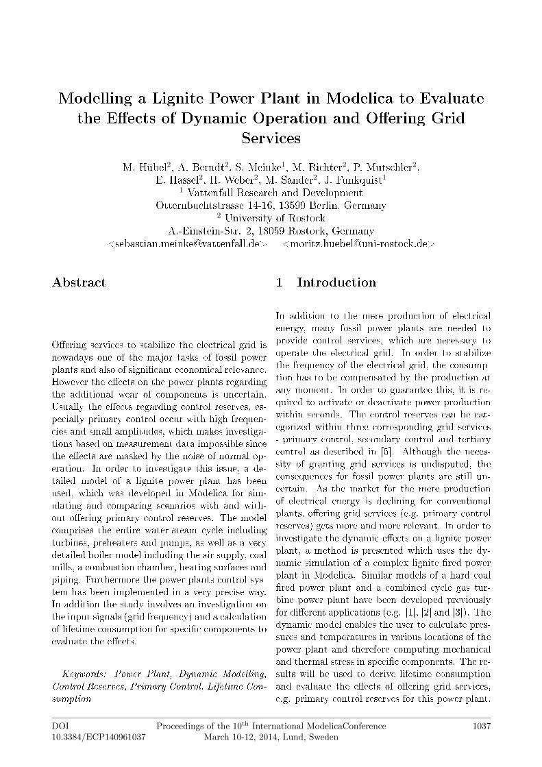
The setpoint of the frequency in the Europeangrid system is 50Hz. The allowed variation ofthe mains frequency in normal mode is between49.8Hz and 50.2Hz. If a failure occurs on the con-sumer or producer side the frequency can changewithin a few seconds. The primary control coun-teracts this. In �gure 1, a typical trend for themains frequency of one day is shown.
0 4 8 12 16 20 24
49.9
49.95
50
50.05
50.1
Time (hour)
Freq
uenc
y (H
z)
Figure 1: Trend of mains frequency of one day
Every power plant involved in the primary con-trol has to provide at least 2% of its e�ective poweras primary control reserve, which has to be avail-able within 30 s.The dynamical behavior of a power plant is
dominated by the dynamics of the steam gener-ator and turbine. In order to provide additionalelectrical power in a short period of time, neededfor primary control, di�erent modes exist:
• Throttling of HP/ IP-valve: The power plantoperates in all operating points with throttledhigh and intermediate pressure steam valves.This grants that the power plant can increaseits output by opening the valves for a posi-tive output demand and decrease its outputby increasing the throttling of the valves.
• Low pressure preheater bypass: In this modethe power plant increases its electrical outputby throttling the valves to the low pressurepreheaters and the feedwater tank. In orderto avoid thermal stress in the low pressurepreheaters the speed of the condensate pumpis decreased. The whole process leads to moresteam in the turbine stages and thus to moreelectrical output. The limits of this mode are
the �lling levels of the condenser and the feed-water tank. For a negative power demand theHP/IP steam valves are throttled as describedin the previous point.
• High pressure preheater bypass: This modeis the same like the low pressure preheaterbypass but uses the high pressure preheatersand the feedwater pump instead.
In order to investigate the in�uence of the pri-mary control for a whole year, it is possible to sim-ulate the whole year with the mains frequency as amodel input, but it takes a lot of time. The imple-mented model has a ratio of real time to simulatedtime of about 1:1 to 1:10. Thus the simulation ofone year would take at least one and a half month.In order to reduce simulation time the data of themains frequency is analyzed and subdivided intocharacteristic signals, distinguishing between:
• changes in mains frequency, which occur everyfull hour, because of the changes of the powerplants schedules
• noise due to the �uctuating consumer load
• power plant outage due to technical issues
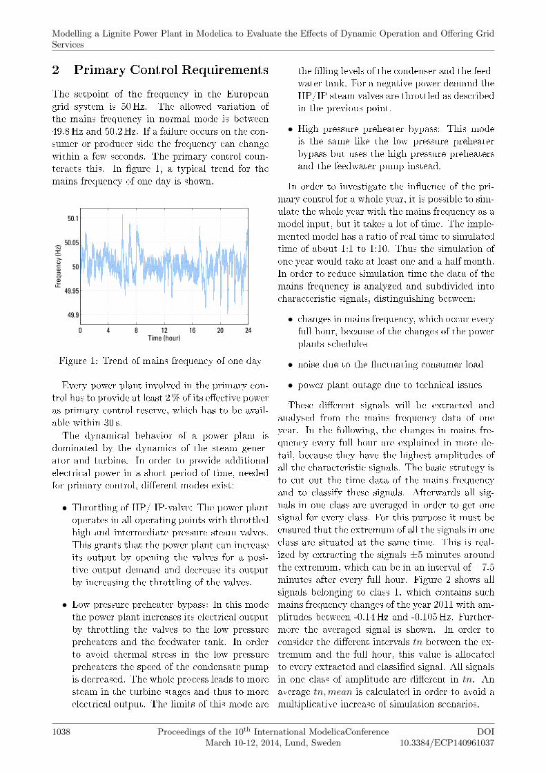
These di�erent signals will be extracted andanalysed from the mains frequency data of oneyear. In the following, the changes in mains fre-quency every full hour are explained in more de-tail, because they have the highest amplitudes ofall the characteristic signals. The basic strategy isto cut out the time data of the mains frequencyand to classify these signals. Afterwards all sig-nals in one class are averaged in order to get onesignal for every class. For this purpose it must beensured that the extremum of all the signals in oneclass are situated at the same time. This is real-ized by extracting the signals ±5 minutes aroundthe extremum, which can be in an interval of +7.5minutes after every full hour. Figure 2 shows allsignals belonging to class 1, which contains suchmains frequency changes of the year 2011 with am-plitudes between -0.14Hz and -0.105Hz. Further-more the averaged signal is shown. In order toconsider the di�erent intervals tn between the ex-tremum and the full hour, this value is allocatedto every extracted and classi�ed signal. All signalsin one class of amplitude are di�erent in tn. Anaverage tn,mean is calculated in order to avoid amultiplicative increase of simulation scenarios.
Modelling a Lignite Power Plant in Modelica to Evaluate the Effects of Dynamic Operation and Offering GridServices
1038 Proceedings of the 10th International ModelicaConferenceMarch 10-12, 2014, Lund, Sweden
DOI10.3384/ECP140961037
0 100 200 300 400 500 600
49.9
49.95
50
50.05
50.1
Time (Seconds)
Freq
uenc
y (H
z)
amplitude class 1: -0.14...-0.105Hz
Figure 2: All signals of one class with the averagedsignal in dark blue
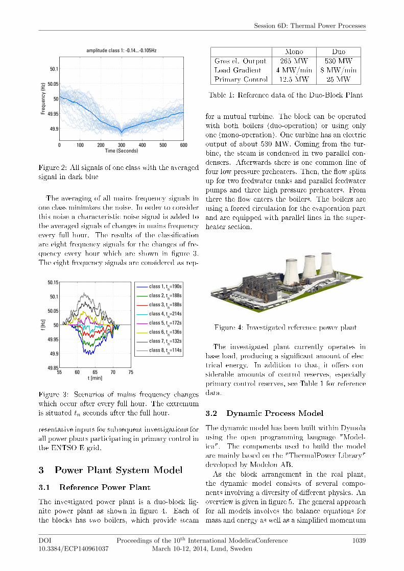
The averaging of all mains frequency signals inone class minimizes the noise. In order to considerthis noise a characteristic noise signal is added tothe averaged signals of changes in mains frequencyevery full hour. The results of the classi�cationare eight frequency signals for the changes of fre-quency every hour which are shown in �gure 3.The eight frequency signals are considered as rep-
55 60 65 70 7549.85
49.9
49.95
50
50.05
50.1
50.15
t [min]
f [Hz
]
class 1, t
n=190s
class 2, tn=188s
class 3, tn=188s
class 4, tn=214s
class 5, tn=172s
class 6, tn=136s
class 7, tn=132s
class 8, tn=114s
Figure 3: Scenarios of mains frequency changeswhich occur after every full hour. The extremumis situated tn seconds after the full hour.
resentative inputs for subsequent investigations forall power plants participating in primary control inthe ENTSO-E grid.
3 Power Plant System Model
3.1 Reference Power Plant
The investigated power plant is a duo-block lig-nite power plant as shown in �gure 4. Each ofthe blocks has two boilers, which provide steam
Mono DuoGros el. Output 265 MW 530 MWLoad Gradient 4 MW/min 8 MW/minPrimary Control 12.5 MW 25 MW
Table 1: Reference data of the Duo-Block Plant
for a mutual turbine. The block can be operatedwith both boilers (duo-operation) or using onlyone (mono-operation). One turbine has an electricoutput of about 530 MW. Coming from the tur-bine, the steam is condensed in two parallel con-densers. Afterwards there is one common line offour low pressure preheaters. Then, the �ow splitsup for two feedwater tanks and parallel feedwaterpumps and three high pressure preheaters. Fromthere the �ow enters the boilers. The boilers areusing a forced circulation for the evaporation partand are equipped with parallel lines in the super-heater section.
Figure 4: Investigated reference power plant
The investigated plant currently operates inbase load, producing a signi�cant amount of elec-trical energy. In addition to that, it o�ers con-siderable amounts of control reserves, especiallyprimary control reserves, see Table 1 for referencedata.
3.2 Dynamic Process Model
The dynamic model has been built within Dymolausing the open programming language "Model-ica". The components used to build the modelare mainly based on the "ThermalPower Library"developed by Modelon AB.As the block arrangement in the real plant,
the dynamic model consists of several compo-nents involving a diversity of di�erent physics. Anoverview is given in �gure 5. The general approachfor all models involves the balance equations formass and energy as well as a simpli�ed momentum
Session 6D: Thermal Power Processes
DOI10.3384/ECP140961037
Proceedings of the 10th International ModelicaConferenceMarch 10-12, 2014, Lund, Sweden
1039
Feedwater-
Tank
Condenser
RH 2
SH 4
SH 3
SHS
Evaporator
Combustion-
chamber
SH 2
RH 1B
RH 1ASH 1
Eco
HP-T LP-TIP-T
Coal Mill
Air-Preheater
Forced-Draft
Fan
Induced-Draft
Fan
Circulation-
Pump
Separator
Feedwater
Pump
HPP 5
HPP 6
HPP 7
LPP 4 LPP 3 LPP 2 LPP 1
Condensate-
Pump
Heating Surface
Combustion Chamber
Turbine
Pumps/Fans
Two-Phase-Tanks
Coal Mills
other modells
Figure 5: Implemented components of reference power plant
equation to calculate pressure drops. Using theseequations as well as speci�c heat transfer assump-tions for conduction, convection and radiation andthe �uid properties for the involved mediums (�uegas, water) a power plant process can be describedon a fundamental basis. A detailed explanation ofphysical backgrounds for all the basic models usedhere can be found in [6]. However the complexpower plant system required some more sophisti-cated models which needed to be developed in or-der to reproduce the plants behaviour in an accu-rate way. One example for such a component is thelignite coal mill as presented in �gure 6. The coalmill is not only responsible for grinding the coalto the desired size, but also for drying the lignite,as the water content of the fuel is usually between50-60 %. As those e�ects have a signi�cant impacton the overall process dynamics, a model had tobe developed to describe the dynamic behaviourof the coal mills.
The coal mill model consists of three main paths.The gas path describes the hot �ue gas which is re-circulated from the combustion chamber. Further-more fresh air with lower temperature is added tocontrol the temperature in the classi�er of the mill.The ventilation e�ect of the mill is represented bya simple fan model based on the speci�c charac-teristic of the mill. The water path represents thewater content of the coal which is evaporated inthe mill. The energy used for evaporation is takenfrom the hot �ue gas. After evaporation, the wateris mixed with the �ue gas. The coal containing aresidual water content of 10-20% is represented by
the coal path.
Raw Coal
Combustion Chamber
Fresh Air
Water
Gas
Dried Coal (containing residual water)
Fan Model
Heat-Transfer
Figure 6: Schematic of the lignite coal mill model
One essential part of the model is the changedlower caloric heating value due to the evaporationof the water. In order to describe this, a simple as-sumption based on [7] leads to reasonable results:
CVx =CV0
(1−XA,0)(1−XW,0)(1−XA,x)(1−XW,x)
(1)
Wherein CV denotes the lower caloric heatingvalue and X the mass content of a speci�c compo-nent (index A for ash, W for water). The indicesx and 0 are representing the state before and be-hind the evaporation stage. The delay time for
Modelling a Lignite Power Plant in Modelica to Evaluate the Effects of Dynamic Operation and Offering GridServices
1040 Proceedings of the 10th International ModelicaConferenceMarch 10-12, 2014, Lund, Sweden
DOI10.3384/ECP140961037
the grinding of the coal has been identi�ed by �t-ting the heat release to the measurement data. [8]gives some values for the delay time in each stageof the mill, which gives a reasonable starting pointfor this optimisation procedure. The water steamcycle has been adapted to a single boiler. Forthe model, components which are actually used byboth boilers are represented as a symmetric partwith the half size. This concerns the models forthe steam turbine, as well as the low pressure pre-heater line.
3.3 Control System
For making simulation-based statements about thein�uence of di�erent power plant operation modesthe thermodynamic model is coupled to a reducedcopy of the origninal power plant control system,which is implemented using the Modelica Stan-dard Library components. The implemented con-trol system uses the currently calculated physicalvalues (i.e. live steam parameter, generated powerat a speci�c coal input) and in a consequence ad-justs set values (e.g. life steam pressure) and ma-nipulated variables (e.g. position of the feed wa-ter valve) for the water-steam cycle. Because ofthis feedback the accuracy and the level of detailsof the modelled processes needs to be reasonablyhigh. Figure 7 is showing the hierarchical struc-ture of the control system, which has been coupledto the process model.
Fresh Air Control Coal Mill Control Feed WaterPump
Control
SeparatorLevel
Control
TurbineControl
Condenser Level
Control
Preheater Level
Control
Air & FuelSystem
Water SteamCycle
Steam Temp-
rature Control
PowerUnit Control
Figure 7: Overview on the control loops imple-mented in the model
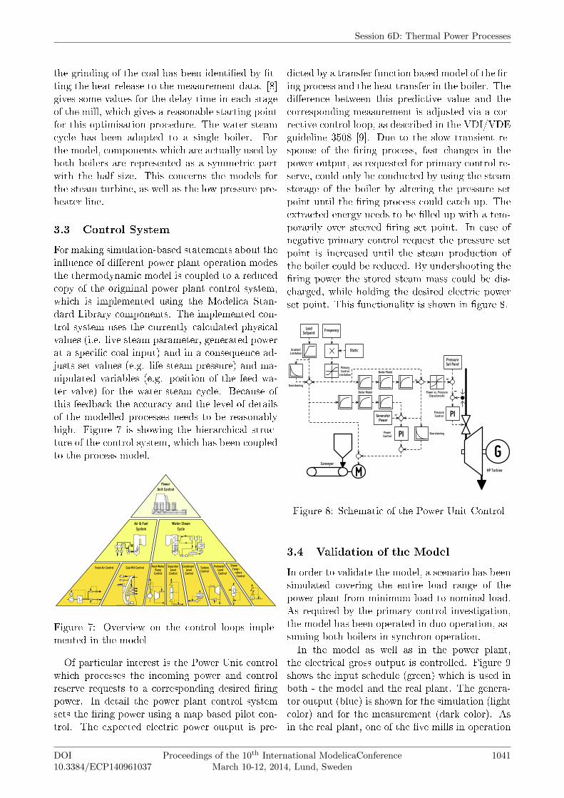
Of particular interest is the Power Unit controlwhich processes the incoming power and controlreserve requests to a corresponding desired �ringpower. In detail the power plant control systemsets the �ring power using a map based pilot con-trol. The expected electric power output is pre-
dicted by a transfer function based model of the �r-ing process and the heat transfer in the boiler. Thedi�erence between this predictive value and thecorresponding measurement is adjusted via a cor-rective control loop, as described in the VDI/VDEguideline 3508 [9]. Due to the slow transient re-sponse of the �ring process, fast changes in thepower output, as requested for primary control re-serve, could only be conducted by using the steamstorage of the boiler by altering the pressure setpoint until the �ring process could catch up. Theextracted energy needs to be �lled up with a tem-porarily over steered �ring set point. In case ofnegative primary control request the pressure setpoint is increased until the steam production ofthe boiler could be reduced. By undershooting the�ring power the stored steam mass could be dis-charged, while holding the desired electric powerset point. This functionality is shown in �gure 8.
PI
-
Conveyor
- -
HP Turbine
G
-
M
Load Setpoint
Frequency
Static
GeneratorPower
Boiler Model
Boiler Model
Power vs. PressureCharacteristic
OversteeringPower Control
PressureSet Point
GradientLimitation
PrimaryControl
Limitation
PIPressureControl
Oversteering
Figure 8: Schematic of the Power Unit Control
3.4 Validation of the Model
In order to validate the model, a scenario has beensimulated covering the entire load range of thepower plant from minimum load to nominal load.As required by the primary control investigation,the model has been operated in duo-operation, as-suming both boilers in synchron operation.In the model as well as in the power plant,
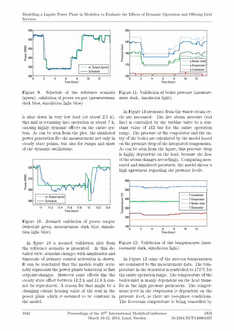
the electrical gross output is controlled. Figure 9shows the input schedule (green) which is used inboth - the model and the real plant. The genera-tor output (blue) is shown for the simulation (lightcolor) and for the measurement (dark color). Asin the real plant, one of the �ve mills in operation
Session 6D: Thermal Power Processes
DOI10.3384/ECP140961037
Proceedings of the 10th International ModelicaConferenceMarch 10-12, 2014, Lund, Sweden
1041
0 2 4 6 8 10 12300
350
400
450
500
550
Time (hour)
Pow
er (M
W)
el. Output (gros)Schedule
Figure 9: Schedule of the reference scenario(green), validation of power output (measurementdark blue, simulation light blue)
is shut down in very low load (at about 2.5 h),this mill is returning into operation at about 7 h,causing highly dynamic e�ects on the entire sys-tem. As can be seen from the plot, the simulatedpower generation �ts the measurement not only insteady state points, but also for ramps and mostof the dynamic oscillations.
11 11.2 11.4 11.6 11.8 12 12.2 12.4
490
500
510
520
Time (hour)
Pow
er (M
W)
el. Output (gros)Schedule
Figure 10: Zoomed validation of power output(schedule green, measurement dark blue, simula-tion light blue)
In �gure 10 a zoomed validation plot fromthe reference scenario is presented. In this de-tailed view, setpoint-changes with amplitudes andtimescale of primary control activation is shown.It can be concluded that the models really accu-ratly represents the power plants behaviour at fastsetpoint-changes. However some e�ects like thesteady state o�set between 11.2 h and 11.8 h can-not be reproduced. A reason for that might be achanging caloric heating value of the coal in thepower plant which is assumed to be constant inthe model.
0 2 4 6 8 10 12160
170
180
190
200
Time (hour)
Pres
sure
(bar
)
p Boiler-Inletp Evaporatorp Livesteam
Figure 11: Validation of boiler pressure (measure-ment dark, simulation light)
In Figure 11 pressures from the water-steam cy-cle are presented. The live steam pressure (redline) is controlled by the turbine valve to a con-stant value of 162 bar for the entire operationrange. The pressure at the evaporator and the en-try of the boiler are calculated by the model basedon the pressure drop of the integrated components.As can be seen from the �gure, this pressure dropis highly dependent on the load, because the �owof the steam changes accordingly. Comparing mea-sured and simulated pressures, the model shows ahigh agreement regarding the pressure levels.
0 2 4 6 8 10 12100
200
300
400
500
600
Time (hour)
Tem
pera
ture
(°C)
T LivesteamT EvaporatorT Boiler-InletT Deaerator
Figure 12: Validation of the temperatures (mea-surement dark, simulation light)
In Figure 12 some of the process temperaturesare compared to the measurement data. The tem-perature in the deaerator is controlled to 174◦C forthe entire operation range. The temperature of theboiler-inlet is manly dependent on the heat trans-fer in the high pressure preheaters. The temper-ature level in the evaporator is dependent on thepressure level, as there are two-phase conditions.The livesteam temperature is being controlled by
Modelling a Lignite Power Plant in Modelica to Evaluate the Effects of Dynamic Operation and Offering GridServices
1042 Proceedings of the 10th International ModelicaConferenceMarch 10-12, 2014, Lund, Sweden
DOI10.3384/ECP140961037
the spray attemperators, however in very low load(between 2.5 and 7 h) the steam temperatures dropdue to a shifting distribution of heat �ux in theboiler and are out of their controlled range.
0 2 4 6 8 10 12120
140
160
180
200
220
Time (hour)
Tem
pera
ture
(°C)
T SimulatedT Mill 1T Mill 2T Mill 4T Mill 5
Figure 13: Validation of the coal mill model (mea-surement dark, simulation light)
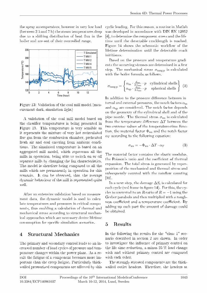
A validation of the coal mill model based onthe classi�er temperatures is being presented inFigure 13. This temperature is very sensible asit represents the mixture of very hot recirculated�ue gas from the combustion chamber, preheatedfresh air and coal entering from ambient condi-tions. The simulated temperature is based on anaggregated mill model, which represents all themills in operation, being able to switch on or o�separate mills by changing the fan characteristics.The model is therefore being compared to all themills which are permanently in operation for thisscenario. It can be observed, that the averagedynamic behaviour of the mill is represented quitewell.
After an extensive validation based on measure-ment data, the dynamic model is used to calcu-late temperatures and pressures in critical compo-nents, thus enabling a calculation of thermal andmechanical stress according to structural mechan-ical approaches which are necessary derive lifetimeconsumption for speci�c simulation scenarios.
4 Structural Mechanics
The primary and secondary control leads to an in-creased number of load cycles of pressure and tem-perature changes within the power plant. As a re-sult the fatigue of a component becomes more im-portant than the creep fatigue. Particularly thick-walled pressurized components are a�ected by this
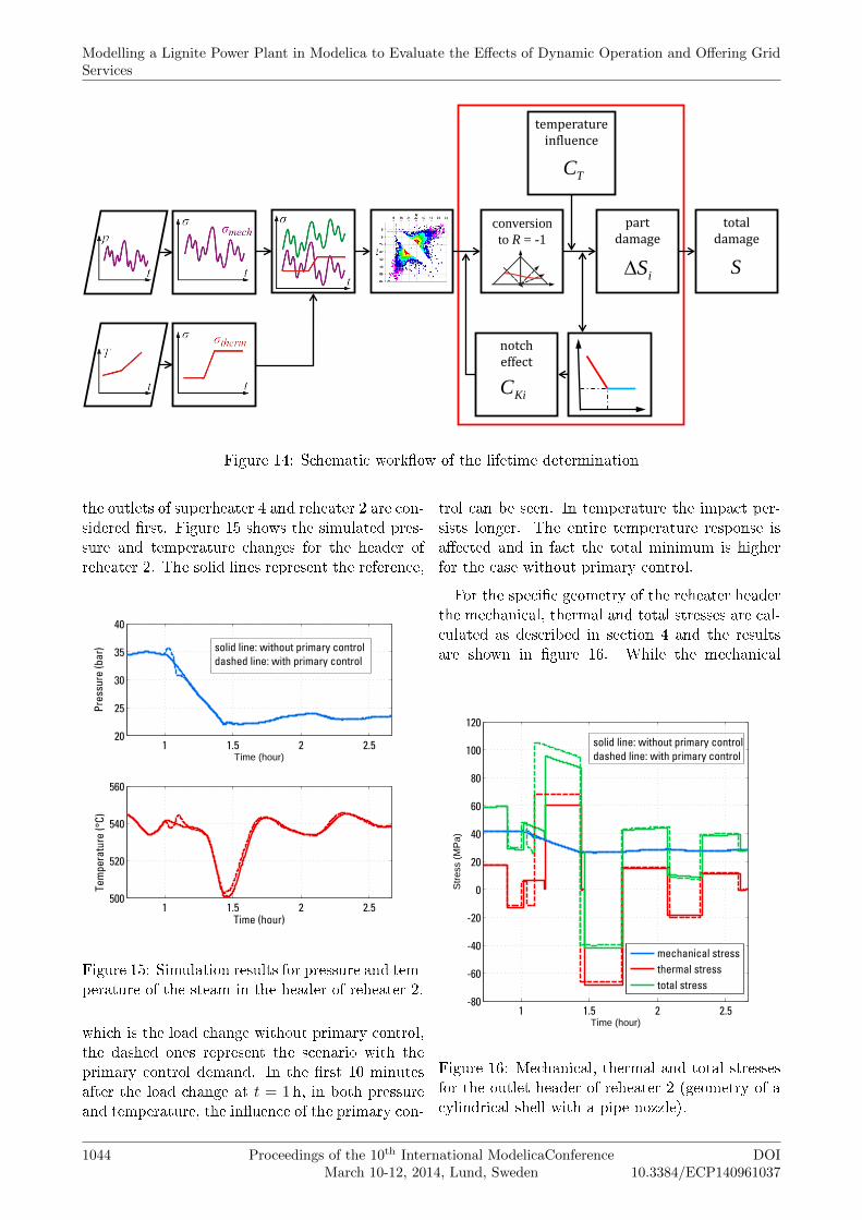
cyclic loading. For this reason, a routine in Matlabwas developed in accordance with DIN EN 12952[4], to determine the component stress and the life-time until the detectable cracklength is reached.Figure 14 shows the schematic work�ow of thelifetime determination until the detectable crackinititiates.Based on the pressure and temperature gradi-
ents the occurring stresses are determined in a �rststep. The mechanical stress σtang p is calculatedwith the boiler formula as follows.
σtang p =
{αm · dms
2·ems· p cylindrical shells
αsp · dms4·ems
· p spherical shells
}(2)
In addition to the pressure di�erence between in-ternal and external pressures, the notch factors αm
and αsp are considered. The notch factor dependson the geometry of the cylindrical shell and of thepipe nozzle. The thermal stress σws is calculatedfrom the temperature di�erence ∆T between thetwo extreme values of the temperature-time func-tion, the material factor Φws and the notch factorαT according to the following equation:
σws = −Φws ·∆T · αT (3)
The material factor contains the elastic modulus,the Poisson's ratio and the coe�cient of thermalexpansion. The total stress is generated by super-position of the mechanical and thermal stress andsubsequently counted with the rain�ow counting[10].In a next step, the damage ∆Si is calculated for
each cycle (red frame in �gure 14). For this, the cy-cles is converted to an R-ratio of R = −1 using theGerber parabola and then multiplied with a rough-ness coe�cient and a temperature coe�cient. Byadding up each part the amount of damage couldbe obtained.
5 Results
In the following the results for the "class 1" sce-nario described in section 2 are shown. In orderto investigate the in�uence of primary control onthe life time reduction, a minus 25 % load changewith and without primary control are comparedwith each other.The strongly stressed components are the thick-
walled outlet headers. Therefore, the headers at
Session 6D: Thermal Power Processes
DOI10.3384/ECP140961037
Proceedings of the 10th International ModelicaConferenceMarch 10-12, 2014, Lund, Sweden
1043
notch effect
temperature influence
part damage
total damage
conversion to R = -1
iS∆
TC
S
KiC
Figure 14: Schematic work�ow of the lifetime determination
the outlets of superheater 4 and reheater 2 are con-sidered �rst. Figure 15 shows the simulated pres-sure and temperature changes for the header ofreheater 2. The solid lines represent the reference,
1 1.5 2 2.520
25
30
35
40
Pres
sure
(bar
)
Time (hour)
1 1.5 2 2.5500
520
540
560
Time (hour)
Tem
pera
ture
(°C)
solid line: without primary controldashed line: with primary control
Figure 15: Simulation results for pressure and tem-perature of the steam in the header of reheater 2.
which is the load change without primary control,the dashed ones represent the scenario with theprimary control demand. In the �rst 10 minutesafter the load change at t = 1 h, in both pressureand temperature, the in�uence of the primary con-
trol can be seen. In temperature the impact per-sists longer. The entire temperature response isa�ected and in fact the total minimum is higherfor the case without primary control.
For the speci�c geometry of the reheater headerthe mechanical, thermal and total stresses are cal-culated as described in section 4 and the resultsare shown in �gure 16. While the mechanical
1 1.5 2 2.5-80
-60
-40
-20
0
20
40
60
80
100
120
Time (hour)
Str
ess
(MP
a)
mechanical stressthermal stresstotal stress
solid line: without primary controldashed line: with primary control
Figure 16: Mechanical, thermal and total stressesfor the outlet header of reheater 2 (geometry of acylindrical shell with a pipe nozzle).
Modelling a Lignite Power Plant in Modelica to Evaluate the Effects of Dynamic Operation and Offering GridServices
1044 Proceedings of the 10th International ModelicaConferenceMarch 10-12, 2014, Lund, Sweden
DOI10.3384/ECP140961037
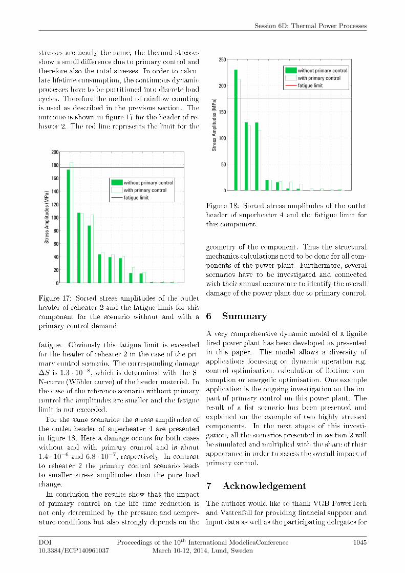
stresses are nearly the same, the thermal stressesshow a small di�erence due to primary control andtherefore also the total stresses. In order to calcu-late lifetime consumption, the continuous dynamicprocesses have to be partitioned into discrete loadcycles. Therefore the method of rain�ow-countingis used as described in the previous section. Theoutcome is shown in �gure 17 for the header of re-heater 2. The red line represents the limit for the
1 2 3 4 5 6 7 8 9 10 110
20
40
60
80
100
120
140
160
180
200
Stre
ss A
mpl
itude
s (M
Pa)
without primary controlwith primary controlfatigue limit
Figure 17: Sorted stress amplitudes of the outletheader of reheater 2 and the fatigue limit for thiscomponent for the scenario without and with aprimary control demand.
fatigue. Obviously this fatigue limit is exceededfor the header of reheater 2 in the case of the pri-mary control scenario. The corresponding damage∆S is 1.3 · 10−8, which is determined with the S-N-curve (Wöhler curve) of the header material. Inthe case of the reference scenario without primarycontrol the amplitudes are smaller and the fatiguelimit is not exceeded.For the same scenarios the stress amplitudes of
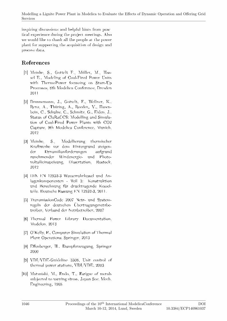
the outlet header of superheater 4 are presentedin �gure 18. Here a damage occurs for both caseswithout and with primary control and is about1.4 · 10−6 and 6.8 · 10−7, respectively. In contrastto reheater 2 the primary control scenario leadsto smaller stress amplitudes than the pure loadchange.In conclusion the results show that the impact
of primary control on the life time reduction isnot only determined by the pressure and temper-ature conditions but also strongly depends on the
1 2 3 4 5 6 7 8 9 10 110
50
100
150
200
250
Stre
ss A
mpl
itude
s (M
Pa)
without primary controlwith primary controlfatigue limit
Figure 18: Sorted stress amplitudes of the outletheader of superheater 4 and the fatigue limit forthis component.
geometry of the component. Thus the structuralmechanics calculations need to be done for all com-ponents of the power plant. Furthermore, severalscenarios have to be investigated and connectedwith their annual occurrence to identify the overalldamage of the power plant due to primary control.
6 Summary
A very comprehensive dynamic model of a lignite�red power plant has been developed as presentedin this paper. The model allows a diversity ofapplications focussing on dynamic operation e.g.control optimisation, calculation of lifetime con-sumption or energetic optimisation. One exampleapplication is the ongoing investigation on the im-pact of primary control on this power plant. Theresult of a �st scenario has been presented andexplained on the example of two highly stressedcomponents. In the next stages of this investi-gation, all the scenarios presented in section 2 willbe simulated and multiplied with the share of theirappearance in order to assess the overall impact ofprimary control.
7 Acknowledgement
The authors would like to thank VGB PowerTechand Vattenfall for providing �nancial support andinput data as well as the participating delegates for
Session 6D: Thermal Power Processes
DOI10.3384/ECP140961037
Proceedings of the 10th International ModelicaConferenceMarch 10-12, 2014, Lund, Sweden
1045
inspiring discussions and helpful hints from prac-tical experience during the project meetings. Alsowe would like to thank all the people at the powerplant for supporting the acquisition of design andprocess data.
References
[1] Meinke, S., Gottelt F., Müller, M., Has-sel E., Modeling of Coal-Fired Power Unitswith ThermoPower focussing on Start-UpProcesses, 8th Modelica Conference, Dresden2011
[2] Brunnemann, J., Gottelt, F., Wellner, K.,Renz, A., Thüring, A., Roeder� V., Hasen-bein, C., Schulze, C., Schmitz, G., Eiden, J.,Status of ClaRaCCS: Modelling and Simula-tion of Coal-Fired Power Plants with CO2Capture, 9th Modelica Conference, Munich,2012
[3] Meinke, S., Modellierung thermischerKraftwerke vor dem Hintergrund steigen-der Dynamikanforderungen aufgrundzunehmender Windenergie- und Photo-voltaikeinspeisung, Dissertation, Rostock,2012
[4] DIN EN 12952-3 Wasserrohrkessel und An-lagenkomponenten - Teil 3: Konstruktionund Berechnung für drucktragende Kessel-teile. Deutsche Fassung EN 12952-3, 2011.
[5] TransmissionCode 2007 Netz- und System-regeln der deutschen Übertragungsnetzbe-treiber, Verband der Netzbetreiber, 2007
[6] Thermal Power Library Documentation,Modelon, 2013
[7] O'Kelly, P., Computer Simulation of ThermalPlant Operations, Springer, 2013
[8] E�enberger, H., Dampferzeugung, Springer2000
[9] VDI/VDE-Guideline 3508, Unit control ofthermal power stations, VDI/VDE, 2003
[10] Matsuishi, M., Endo, T., Fatigue of metalssubjected to varying stress, Japan Soc. Mech.Engineering, 1968
Modelling a Lignite Power Plant in Modelica to Evaluate the Effects of Dynamic Operation and Offering GridServices
1046 Proceedings of the 10th International ModelicaConferenceMarch 10-12, 2014, Lund, Sweden
DOI10.3384/ECP140961037


![V.S LIGNITE POWER Pvt. Ltd [Gurha East Lignite Mine (1 MPTA)] · V.S LIGNITE POWER Pvt. Ltd [Gurha East Lignite Mine (1 MPTA)] AT VILLAGE-GURHA, KOLAYAT, BIKANER, ... Embankment has](https://img.pdfslide.us/doc/110x75/5e8c64539924dc7ac37938bd/vs-lignite-power-pvt-ltd-gurha-east-lignite-mine-1-mpta-vs-lignite-power.jpg)