ModelingandAnalysisofCongestion intheDesignofFacilityLayouts · ModelingandAnalysisofCongestion intheDesignofFacilityLayouts ... sign tends to ignore the potential impact of facility

Modeling and Analysis of Congestionin the Design of Facility Layouts

Saifallah BenjaafarDivision of Industrial Engineering, Department of Mechanical Engineering,

University of Minnesota, Minneapolis, Minnesota [email protected]

Reducing manufacturing lead times and minimizing work-in-process (WIP) inventoriesare the cornerstones of popular manufacturing strategies such as Lean, Quick Response,

and Just-in-Time Manufacturing. In this paper, we present a model that captures the rela-tionship between facility layout and congestion-related measures of performance. We use themodel to introduce a formulation of the facility layout design problem where the objective isto minimize work-in-process (WIP). In contrast to some recent research, we show that layoutsobtained using a WIP-based formulation can be very different from those obtained usingthe conventional quadratic assignment problem (QAP) formulation. For example, we showthat a QAP-optimal layout can be WIP-infeasible. Similarly, we show that two QAP-optimallayouts can have vastly different WIP values. In general, we show that WIP is not mono-tonic in material-handling travel distances. This leads to a number of surprising results. Forinstance, we show that it is possible to reduce overall distances between departments butincrease WIP. Furthermore, we find that the relative desirability of a layout can be affectedby changes in material-handling capacity even when travel distances remain the same. Weexamine the effect of various system parameters on the difference in WIP between QAP- andWIP-optimal layouts. We find that although there are conditions under which the differencein WIP is significant, there are those under which both layouts are WIP-equivalent.(Facility Layout; Queueing Networks; Quadratic Assignment Problem; Material Handling; Perfor-mance Evaluation)

1. IntroductionReducing manufacturing lead times and minimizingwork-in-process (WIP) inventories are the corner-stones of popular manufacturing strategies such asLean, Quick Response, and Just-in-Time Manufactur-ing (Hopp and Spearman 2000, Suri 1998, Womackand Jones 1996). Although various facets of the man-ufacturing function have been redesigned in recentyears to support lead-time and inventory reduction,the physical organization and layout of manufactur-ing facilities have continued to be largely guidedby more traditional concerns of efficiency and cost(Benjaafar et al. 2002). This approach to facility de-sign tends to ignore the potential impact of facility

layout and material handling on short-term opera-tional effectiveness. It also does not account for thepossibility of using facility design strategically tosupport a manufacturing firms’ need for agility andresponsiveness.In this paper, we show that physical layout of

facilities can impact operational performance in sig-nificant ways, as measured by lead time, WIP, orthroughput. We also show that the traditional facil-ity design criterion can be a poor indicator of thisperformance. More importantly, we identify charac-teristics of layouts that tend to reduce lead time andWIP and improve throughput. Because operationalperformance is driven by system congestion, which

0025-1909/02/4805/0679$5.001526-5501 electronic ISSN

Management Science © 2002 INFORMSVol. 48, No. 5, May 2002 pp. 679–704

BENJAAFARModeling and Analysis of Congestion

is itself a function of system capacity and variability,we introduce a model that captures the relationshipbetween layout and congestion. We use the model toexamine the effect of layout on capacity and variabil-ity and derive insights that can be used to generatewhat might be termed as agile or quick response lay-outs.In our analysis, we focus on WIP as our primary

measure of congestion. However, by virtue of Little’slaw, this could also be related to both lead time andthroughput. In our analysis, we assume that capac-ity decisions have already been made. Therefore, ourobjective is to determine a layout that minimizes WIPgiven fixed material-handling capacity. Our modelcan, however, be used to solve problems where bothmaterial-handling capacity and layout are decisionvariables, so that the objective is to minimize bothinvestment and congestion costs. Alternatively, themodel can be used to formulate problems where theobjective is to minimize one type of cost subject to aconstraint on the other.Our work is in part motivated by two recent

papers by Fu and Kaku (1997a, 1997b) in which theypresent a plant layout problem formulation for job-shop-like manufacturing systems where the objectiveis to minimize average work-in-process. In partic-ular, they investigate conditions under which thefamiliar quadratic assignment problem (QAP) for-mulation, where the objective is to minimize aver-age material-handling costs, also minimizes averagework-in-process. By modeling the plant as an openqueueing network, they show that under a set ofassumptions the problem reduces to the quadraticassignment problem. Using a simulation of an exam-ple system, they found that the result apparentlyholds under much more general conditions than areassumed in the analytical model.To obtain a closed-form expression of expected WIP,

Fu and Kaku (1997b) make the following assump-tions: (1) external part type arrival processes intothe system are Poisson; (2) processing times at adepartment are i.i.d. exponential; (3) material han-dling is carried out via discrete material-handlingdevices, such as forklifts or automated guided vehi-cles (AGV), (4) travel times of the material-handlingdevices are exponentially distributed, (5) input and

output buffer sizes at departments are sufficientlylarge so that blocking is negligible, and (6) servicediscipline is first come, first served (FCFS). In mod-eling travel times, they ignore empty travel by thematerial-handling devices and account only for fulltrips. These assumptions allow them to treat the net-work as a Jackson queueing network—i.e., a net-work of independent M/M/n queues—for which aclosed-form analytical expression of average WIP isavailable. They show that WIP accumulation at theprocessing departments—at both the input and out-put buffers—is always independent of the layout andthat travel times are a linear transformation of theaverage distance traveled by the material-handlingsystem when full. Because the measure of material-handling cost used in the QAP formulation is itselfa linear function of the same average travel distance,they show that the queueing and QAP formulationsare equivalent.In this paper, we show that when some of the

assumptions used by Fu and Kaku are relaxed, theirkey observation regarding the equivalence of the twoformulations is not always valid. In fact, under gen-eral conditions, we show that layouts generated usingthe queueing-based model can be very different fromthose obtained using the conventional QAP formu-lation. More importantly, we show that the choiceof layout does have a direct impact on WIP accu-mulation at both the material-handling system andat the individual departments, and that the behaviorof expected WIP is not necessarily monotonic in theaverage distance traveled by the material-handlingdevice. This leads to a number of surprising andcounterintuitive results. In particular, we show thatreducing overall distances between departments canincrease WIP. We also show that the desirability ofa layout can be affected by non-material-handlingfactors, such as department, utilization levels, vari-ability in processing times at departments, and vari-ability in product demands. In general, we find theobjective function used in the QAP formulation tobe a poor indicator of WIP. For example, we showthat a QAP-optimal layout can be WIP-infeasible—i.e., it results in infinite WIP. Similarly, we show thattwo QAP-optimal layouts can have vastly different

680 Management Science/Vol. 48, No. 5, May 2002


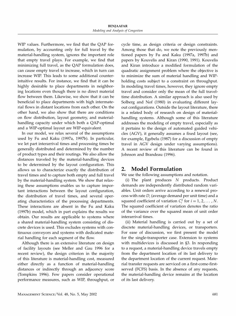
WIP values. Furthermore, we find that the QAP for-mulation, by accounting only for full travel by thematerial-handling system, ignores the important rolethat empty travel plays. For example, we find thatminimizing full travel, as the QAP formulation does,can cause empty travel to increase, which in turn canincrease WIP. This leads to some additional counter-intuitive results. For instance, we find that it can behighly desirable to place departments in neighbor-ing locations even though there is no direct materialflow between them. Likewise, we show that it can bebeneficial to place departments with high intermate-rial flows in distant locations from each other. On theother hand, we also show that there are conditionson flow distribution, layout geometry, and material-handling capacity under which both a QAP-optimaland a WIP-optimal layout are WIP-equivalent.In our model, we relax several of the assumptions

used by Fu and Kaku (1997a, 1997b). In particular,we let part interarrival times and processing times begenerally distributed and determined by the numberof product types and their routings. We also allow thedistances traveled by the material-handling devicesto be determined by the layout configuration. Thisallows us to characterize exactly the distribution oftravel times and to capture both empty and full travelby the material-handling system. We show that relax-ing these assumptions enables us to capture impor-tant interactions between the layout configuration,the distribution of travel times, and several oper-ating characteristics of the processing departments.These interactions are absent in the Fu and Kaku(1997b) model, which in part explains the results weobtain. Our results are applicable to systems wherea shared material-handling system consisting of dis-crete devices is used. This excludes systems with con-tinuous conveyors and systems with dedicated mate-rial handling for each segment of the flow.Although there is an extensive literature on design

of facility layouts (see Meller and Gau 1996 for arecent review), the design criterion in the majorityof this literature is material-handling cost, measuredeither directly as a function of material-handlingdistances or indirectly through an adjacency score(Tompkins 1996). Few papers consider operationalperformance measures, such as WIP, throughput, or

cycle time, as design criteria or design constraints.Among those that do, we note the previously men-tioned papers by Fu and Kaku (1997a, 1997b) andpapers by Kouvelis and Kiran (1990, 1991). Kouvelisand Kiran introduce a modified formulation of thequadratic assignment problem where the objective isto minimize the sum of material handling and WIP-holding costs subject to a constraint on throughput.In modeling travel times, however, they ignore emptytravel and consider only the mean of the full travel-time distribution. A similar approach is also used bySolberg and Nof (1980) in evaluating different lay-out configurations. Outside the layout literature, thereis a related body of research on design of material-handling systems. Although some of this literatureaddresses the modeling of empty travel, especially asit pertains to the design of automated guided vehi-cles (AGV), it generally assumes a fixed layout (see,for example, Egebelu (1987) for a discussion of emptytravel in AGV design under varying assumptions).A recent review of this literature can be found inJohnson and Brandeau (1996).

2. Model FormulationWe use the following assumptions and notation.(i) The plant produces N products. Product

demands are independently distributed random vari-ables. Unit orders arrive according to a renewal pro-cess with rateDi (average demand per unit time) and asquared coefficient of variation C2

i for i = 1�2� �N .The squared coefficient of variation denotes the ratioof the variance over the squared mean of unit orderinterarrival times.(ii) Material handling is carried out by a set of

discrete material-handling devices, or transporters.For ease of discussion, we first present the modelfor the single-transporter case. Extension to systemswith multidevices is discussed in §3. In respondingto a request, a material-handling device travels emptyfrom the department location of its last delivery tothe department location of the current request. Mate-rial transfer requests are serviced on a first-come-first-served (FCFS) basis. In the absence of any requests,the material-handling device remains at the locationof its last delivery.

Management Science/Vol. 48, No. 5, May 2002 681


(iii) The travel time between any pair of locationsk and l, tkl, is assumed to be deterministic and isgiven by tkl = dkl/v, where dkl is the distance betweenlocations k and l and v is the speed of the material-handling transporter.(iv) Products are released to the plant from a

loading department and exit the plant through anunloading (or shipping) department. Departments areindexed from i= 0 toM+1, with the indices i= 0 andM+1 denoting, respectively, the loading and unload-ing departments.(v) The plant consists of M processing depart-

ments, with each department consisting of a singleserver (e.g., a machine) with ample storage for work-in-process. Jobs in the queue are processed in first-come-first-served order. The amount of material flow,�ij , between a pair of departments i and j is deter-mined from the product routing sequence and theproduct demand information. The total amount ofworkload at each department is given by:

�i =M∑k=0

�ki =M+1∑j=1

�ij for i = 1�2� �m� (1)

�0 = �M+1 =N∑i=1

Di� and (2)

�t =M∑i=0

M+1∑j=1

�ij� (3)

where �t is the workload for the material-handlingsystem.(vi) Processing times at each department are inde-

pendent and identically distributed with an expectedprocessing time E�Si� and a squared coefficient of vari-ation C2

sifor i = 0�1� �M + 1 (the processing time

distribution is determined from the processing timesof the individual products).(vii) There are K locations to which departments

can be assigned. A layout configuration correspondsto a unique assignment of departments to locations.We use the vector notation x = �xik�, where xik = 1 ifdepartment i is assigned to location k and xik = 0 oth-erwise, to differentiate between different layout con-figurations. The number of locations is assumed to begreater than or equal to the number of departments.

We model the plant as an open network of GI/G/1queues, with the material-handling system being acentral server queue. Note that because parts aredelivered to the departments by the material-handlingsystem, the operating characteristics of the material-handling system, such as utilization and travel-timedistribution, directly affect the interarrival time distri-bution of parts to the departments. Similarly, since thequeue for the material-handling system consists of thedepartment output buffers, the interarrival time dis-tribution to this queue is determined by the departureprocess from the departments, which is in turn deter-mined by the operating characteristics of the depart-ments. Therefore, there is a close coupling betweenthe inputs and outputs of the processing departmentsand the material-handling system. In our model, weexplicitly capture this coupling and show that thereexists a three-way interaction between the departmentoperating characteristics, the operating characteristicsof the material-handling system, and the layout con-figuration, and that this interaction has a direct effecton WIP accumulation.In order to show this effect, let us first char-

acterize the travel-time distribution. In respondingto a material-transfer request, the material-handlingdevice performs an empty trip from its current loca-tion (the location of its last delivery), at some depart-ment r , followed by a full trip from the origin of thecurrent request, say department i, to the destinationof the transfer request at a specified department j (seeFigure 1). The probability distribution prij of an emptytrip from r to i followed by a full trip from i to j is,therefore, given by:

prij =M∑k=0

pkrpij� (4)

where pij is the probability of a full trip from depart-ment i to department j, which can be obtained as

pij =�ij∑M

i=0∑M+1

j=1 �ij

(5)

We show in §3 that Expressions (4) and (5) are alsovalid for systems with multiple transporters. Given alayout configuration x, the time to perform an emptytrip from department r to department i followed by



Figure 1 Empty and Full Travel in a System with Discrete Material Handling Devices

2

Output bufferInput buffer

Processing department

Empty trip from destination of previousdelivery to origin of current request

Full trip from the origin of currentrequest to its destination department

Material handling device

3

4

1

a full trip to department j is given by trij �x�= tri�x�+tij �x�, where

tij �x�=K∑

k=1

K∑l=1

xikxjldkl/v (6)

and is the travel time from department i to depart-ment j. From (4)–(6), we can obtain the mean andvariance of travel time as follows:

E�St� =M+1∑r=1

M∑i=0

M+1∑j=1

prij trij �x�

=M+1∑r=1

M∑i=0

M+1∑j=1

M∑k=0

(�kr�ij/�

2t

)trij �x�� (7)

and

Var �St�= E(S2t)−E�St�

2� (8)

where

E(S2t) = M+1∑

r=1

M∑i=0

M+1∑j=1

prij(trij �x�

)2

=M+1∑r=1

M∑i=0

M+1∑j=1

M∑k=0

(�kr�ij/�

2t

)(trij �x�

)2� (9)

and

trij �x� =∑k

∑l

∑s

xrkxilxjs�dkl+dls�/v

= ∑k

∑l

xrkxildkl/v+∑l

∑s

xilxjsdls/v (10)

We can also obtain the average utilization of thematerial-handling system, �t , as:

�t = �tE�St�=M+1∑r=1

M∑i=0

M+1∑j=1

M∑k=0

��kr�ij/�t��tri�x�+ tij �x��

(11)

which can be simplified as:

�t =M+1∑r=1

M∑i=0

��r�i/�t�tri�x�+M∑i=0

M+1∑j=1

�ijtij �x� (12)

or equivalently,

�t = �et +�

ft � (13)

where

�et =

M+1∑r=1

M∑i=0

��r�i/�t�tri�x� (14)



corresponds to the utilization of the material-handlingsystem due to empty travel, and

�ft =

M∑i=0

M+1∑j=1

�ijtij �x� (15)

is the utilization of the material-handling system dueto full travel.From the above expressions, we can see that the

travel-time distribution is determined by the lay-out configuration and that this distribution is notnecessarily exponential. As a result, the arrival pro-cess to the departments is not always Poisson dis-tributed, even if external arrivals are Poisson andprocessing times are exponential. This means thatour system cannot be treated, in general, as a net-work of M/M/1 queues. Unfortunately, exact analyt-ical expressions of performance measures of interest,such as expected WIP, expected time in system, andtime in queue, are difficult to obtain for queues withgeneral interarrival and processing time distributions.Therefore, to estimate these measures of performancewe resort to network decomposition and approxi-mation techniques, where each department, as wellas the material-handling system, is treated as beingstochastically independent, with the arrival process toand the departure process from each department andthe material-handling system being approximated byrenewal processes. Furthermore, we assume that twoparameters, mean and variance, of the job interar-rival and processing time distributions are sufficientto estimate expected WIP at each department. Thedecomposition and approximation approach has beenwidely used to analyze queueing networks in a vari-ety of contexts (Bitran and Dasu 1992, Bitran andTirupati 1989, Buzacott and Shanthikumar 1993, Whitt1983a). A number of good approximations have beenproposed by several authors (see Bitran and Dasu1992 for a recent review). In this paper, the approxi-mations we use have been first proposed by Kraemerand Langenbach-Belz (1976) and later refined byWhitt (1983a, 1983b) and shown to perform well overa wide range of parameters (Buzacott and Shanthiku-mar 1993, Whitt 1983b). The approximations coincidewith the exact analytical results obtained by Fu andKaku for the special case of Poisson arrival and expo-nential processing/travel times. Because in layout

design our objective is primarily to obtain a rankedordering of different layout alternatives, approxima-tions are sufficient as long as they guarantee accuracyin the ordering of these alternatives. Approximationsare also adequate when we are primarily interested,as we are in this paper, in the qualitative behavior ofthe performance measures. Comparisons of our ana-lytical results with results obtained using simulationare discussed in §4.Under a given layout, expected WIP at each depart-

ment i (i= 0�1� �M+1) is approximated as follows:

E�WIPi�=�2i(C2

ai+C2

si

)gi

2�1−�i�+�i� (16)

where �i = �iE�Si� is the average utilization of depart-ment i, C2

aiand C2

siare, respectively, the squared coef-

ficients of variation of job interarrival and processingtimes, and

gi ≡ gi

(C2

ai�C2

si� �i

)

=exp

[−2�1−�i��1−C2ai�2

3�i�C2ai+C2

si�

]if C2

ai< 1�

1 if C2ai≥ 1

(17)

Similarly, expected WIP at the material-handlingsystem is approximated by:

E�WIPt�=�2t(C2

at+C2

st

)gt

2�1−�t�+�t (18)

Note that �t and �i must be less than one for expectedwork-in-process to be finite. The squared coefficientsof variation can be approximated as follows (Buzacottand Shanthikumar 1993, Whitt 1983a):

C2ai= ∑

j �=i

�j p̂ji

�i

�p̂jiC2di+ �1−pji��

+ �0#i

�i

�#iC2a0+ �1−#i�� and (19)

C2di= �2i C

2si+ �1−�2i �C

2ai� (20)

where C2diis the squared coefficient of interdeparture

time from department i, p̂ij is the routing probabil-ity from node i to node j (nodes include depart-ments and the material handling device), #i is thefraction of external arrivals that enter the network



through node i, and 1/�0 and C2a0are, respectively,

the mean and squared coefficient of variation of theexternal job interarrival times. In our case, #0 = 1 and#i = 0 for all others since all jobs enter the cell atthe loading department. The routing probability fromdepartments i= 0 throughM to the material-handlingsystem is always one, that from the material-handlingsystem to departments j = 1 through M +1 is

p̂tj =∑M+1

i=0 �ij∑Mi=0∑M+1

j=0 �ij

� (21)

and to the loading department (j = 0) is zero. Partsexit the cell from department M + 1 (unloadingdepartment) so that all the routing probabilities fromthat department are zero. Substituting these probabil-ities in the above expression, we obtain:

C2a0=

N∑i=1

(Di

/ N∑i=1

Di

)C2

i � (22)

C2at=

M∑i=0

��i/�t�C2di=

M∑i=0

$iC2di� and (23)

C2ai= $iC

2dt+1−$i for i = 1�2� �M +1� (24)

where $i = �i/�t . Equalities (22)–(24), along with (20),can be simultaneously solved to yield:

C2ai= $i

(�2t C

2st+ �1−�2t �C

2at

)+1−$i�

for i = 1�2� �M +1� and (25)

C2at=(

M∑i=0

$i�2i C

2si+

M∑i=1

$i�1−�2i ��1−$i�

+M∑i=1

$2i �1−�2i ��

2t C

2st+$0�1−�20�C

2a0

)

/(1−

M∑i=1

$2i �1−�2i ��1−�2t �

) (26)

From the expression of expected WIP, we can obtainadditional measures of performance. For example, byvirtue of Little’s law, expected flow time throughdepartment i (i = 0�, is simply E�Fi� = E�WIPi�/�i

and expected total flow time in system is E�F � =E�WIP�/�D1+· · ·+DN�, where

E�WIP�=M+1∑i=0

E�WIPi�+E�WIPt�

is total expected WIP in the system. We can alsoobtain expected flow time in the system for a specificproduct j as:

E�F �j��=M+1∑i=0

nijE�Fi��

where nij is the number of times product j visitsdepartment i.Any of the above performance measures could be

used as a criterion in layout design. In the remain-der of this article, we limit ourselves to expected totalWIP. However, the analysis can be extended to othermeasures. The layout design problem can be formu-lated as:

Minimize E�WIP�=M+1∑i=0

E�WIPi�+E�WIPt� (27)

subject to:K∑

k=1xik = 1 i = 0�2� �M +1� (28)

M+1∑i=0

xik = 1 k = 1�2� �K� (29)

�t ≤ 1� (30)

xik = 0�1 i = 0�2� �M +1&

k = 1�2� �K (31)

The above formulation shares the same constraints,Constraints (28), (29), and (31), as the QAP formu-lation. Constraints (28) and (29) ensure, respectively,that each department is assigned to one locationand each location is assigned to one department. Werequire an additional constraint, Constraint (30), toensure that a selected layout is feasible and will notresult in infinite work-in-process. As in the QAP for-mulation, we assume K = M + 2. The case whereK >M +2 can be handled by introducing dummydepartments with zero input and output flows. Theobjective function is, however, different from that ofthe QAP. In the conventional QAP, the objective func-tion is a positive linear transformation of the expectedfull travel time and is of the form:

Minimize z=∑i

∑j

∑k

∑l

xikxjl�ijdkl (32)



Therefore, a solution that minimizes average fulltravel time between departments is optimal. Becauseexpected WIP is not, in general, a linear function ofaverage full travel time, the solutions obtained by thetwo formulations, as we show in the next section,can be different. However, a special case where thetwo formulations lead to the same solution is the oneconsidered by Fu and Kaku, where all interarrival,processing, and transportation times are assumed tobe exponentially distributed and empty travel time isnegligible. In this case, we have C2

ai= C2

si= 1, for i =

0�1� �M+1, which when substituted in the expres-sion of expected WIP, while ignoring empty travel,leads to:

E�WIP�=M+1∑i=0

�i

1−�i

+ �t

1−�t

� (33)

with

�t =∑i

∑j

∑k

∑l

�ijxikxjldkl/v (34)

Since only E�WIPt� is a function of the layout (giventhe exponential assumption, the arrival process tothe departments is always Poisson regardless of thelayout configuration), and since E�WIPt� is strictlyincreasing in �t , any solution that minimizes �t alsominimizes the overall WIP. Noting that �t is mini-mized by minimizing z =∑

i

∑j

∑k

∑l �ijxikxjldkl, we

can see that minimizing z also minimizes expectedWIP. In the next section, we show that when we either(1) account for empty travel or (2) relax the exponen-tial assumption regarding interarrival, processing, ortravel times (as we do in our model), the equivalencebetween the QAP and the queueing-based model doesnot hold any longer.The quadratic assignment problem has been shown

to be NP-hard (Pardalos and Wolkowicz 1994).Since the objective function in (27) is a nonlin-ear transformation of that of the QAP, the formu-lation in (27)–(31) also leads to an NP-hard prob-lem. Although for relatively small problems implicitenumeration (e.g., branch and bound) can be usedto solve the problem to optimality (Pardalos andWolkowicz 1994), for most problems we must resortto a heuristic solution approach. Several heuristics

have been proposed for solving the QAP (see Parda-los and Wolkowicz 1994 for a recent review) and anyof these could be used to solve our model as well. Ina software implementation of the formulation in (27)–(31), Yang and Benjaafar (2001) used both implicitenumeration and a modified 2-opt heuristic, similarto the one proposed by Fu and Kaku (1997a), to solvethe problem. In this paper, we limit our discussionmostly to layouts where the QAP-optimal layout iseasily identified.

3. Systems with MultipleTransporters

For a system with multiple transporters, the travel-time distribution is affected by the dispatching policyused to select a transporter whenever two or more areavailable to carry out the current material-handlingrequest. Analysis of most dispatching policies is dif-ficult. In this section, we treat the mathematicallytractable case of randomly selecting a device whentwo or more are idle. Although not optimal, this pol-icy does yield a balanced workload allocation amongthe different devices. Assuming transfer requests areprocessed on a first-come-first-served basis, this pol-icy also ensures an assignment of transporters todepartments proportional to the departments’ work-loads. As in the single-transporter case, we assumethat vehicles remain at the location of their last deliv-ery if there are no pending requests.In order to characterize the probability distribution

of travel time in a system with nt transporters (nt > 1),we need to first obtain the probability prij of an emptytrip from department r followed by a full trip fromdepartment i to j. The probability of a full trip from ito j is still given by (5). The probability of an emptytrip from r can be written as follows:

Prob(empty trip from r)

=nt∑

ns=1

ns∑nr=1

�Prob (selecting transporter at r nr

and ns) Prob �nr ns� Prob �ns�} (35)

where Prob(selecting transporter at r nr and ns) refersto the probability of selecting one of the idle vehiclesat department r given that there are nr idle vehicles at



r and ns total idle vehicles in the system, Prob (nr ns)is the probability of having nr idle vehicles at depart-ment r where nr = 1�2� �ns , given that there are ns

idle vehicles in the system, and Prob(ns) is the proba-bility of having ns idle vehicles in the system, wherens = 1�2� �nt . It is straightforward to show that

Prob(selecting transporter at r nr and ns)

= nr/ns� and (36)

Prob�nr ns�=(ns

nr

)pnrr �1−pr�

ns−nr � (37)

where pr is the probability of an idle vehicle being atdepartment r which is given by:

pr =M∑i=0

pir =M∑i=0

�ir

/ M∑i=0

M+1∑j=1

�ij (38)

We can now write the probability prij as

prij ={ nt∑ns=1

ns∑nr=1

nr

ns

(ns

nr

)pnrr �1−pr�

ns−nrProb�ns�

}pij

(39)

or equivalently as

prij={ nt∑ns=1

�1/ns�Prob�ns�ns∑

nr=1nr

(ns

nr

)pnrr �1−pr�

ns−nr

}pij

(40)

Noting that

ns∑nr=1

nr

(ns

nr

)pnrr �1−pr�

ns−nr = nspr� and (41)

nt∑ns=1

Prob�ns�= 1�

yields to

prij ={ nt∑ns=1

Prob�ns�pr

}pij = prpij� (42)

which is the same as in the single-transporter case (aresult due to the random nature of the selection rule).One could also have argued directly that given theprobabilistic routing and the random selection rulefor the material-handling system, the probability ofan empty trip from r to i followed by a full trip from

i to j would depend only on the workloads assignedto each department and not on the number of trans-porters.The mean and variance of travel time can now be

obtained as in (7) and (8). Expected WIP due to thetransporters can be obtained using approximationsfor a GI/G/nt queue. Similarly, the departure pro-cess from the transporters can be approximated as adeparture process from a GI/G/nt queue, which canthen be used to characterize the arrival process to thedepartments and the transporters as in (25)–(26). Adetailed analysis and software implementation of thisapproach can be found in Yang and Benjaafar (2001).In §5, we examine the effect of the number of trans-porters on layout performance.

4. Model Analysis and InsightsIn this section, we show that layouts obtained usinga WIP-based formulation can be very different fromthose using the QAP formulation. We trace these dif-ferences to two major factors: empty travel and travel-time variability.

4.1. The Effect of Empty TravelIn the following set of observations, we examine theimpact of empty travel. We show that a layout thatminimizes �f does not necessarily minimize �e, andconsequently, a layout that minimizes �f does notnecessarily minimize WIP. In fact, we show that aQAP-optimal layout (i.e., a layout that minimizes �f )is not even guaranteed to be feasible. More generally,we show that two QAP-optimal layouts can resultin different WIP values. Furthermore, under certainconditions we find that WIP is reduced more effec-tively by reducing empty travel, even if this increasesfull travel. This means that sometimes it can be desir-able to place departments in neighboring locationseven though there is no direct material flow betweenthem. This also means that it can be beneficial to placedepartments with high intermaterial flows in distantlocations from each other.Observation 1. A layout that minimizes full travel

does not necessarily minimize WIP.The result follows from noting that reducing �f can

increase �e. If the increase in �e is sufficiently large,



Figure 2 Data for Example Layout

0 1 2 3

7 6 5 4

8 9 10 11

(a) Available department locations

From/To 0 1 2 3 4 5 6 7 8 9 10 110 0 1 2 3 4 3 2 1 2 3 4 51 1 0 1 2 3 2 1 2 3 2 3 42 2 1 0 1 2 1 2 3 4 3 2 33 3 2 1 0 1 2 3 4 5 4 3 24 4 3 2 1 0 1 2 3 4 3 2 15 3 2 1 2 1 0 1 2 3 2 1 26 2 1 2 3 2 1 0 1 2 1 2 37 1 2 3 4 3 2 1 0 1 2 3 48 2 3 4 5 4 3 2 1 0 1 2 39 3 2 3 4 3 2 1 2 1 0 1 210 4 3 2 3 2 1 2 3 2 1 0 111 5 4 3 2 1 2 3 4 3 2 1 0

(b) Distances between department locations

Departments Average processing time0 181 182 63 64 185 186 187 188 69 610 1811 18

(c) Department average processing times

an increase in expected WIP can then follow. We illus-trate this result using the following example. Considera system consisting of 12 locations and 12 depart-ments arranged in a 3×4 grid as shown in Figure 2(a).

Departments are always visited by all products inthe following sequence: 0→ 1→ 2→ 3→ 2→ 3→2 → 3 → 4 → 5 → 6 → 7 → 8 → 9 → 8 → 9 → 8 →9→ 10→ 11. The distance matrix between locations



Figure 3 Example Layouts

8 9 10 11

7 6 5 4

3210

(a) Layout x1ρt = 0.990, ρf = 0.311, ρe = 0.679,

E(WIPt) = 58.37, E(WIP) = 69.53

7 8 9 10

11 2 3 4

5610

(b) Layout x2ρ ρ ρ ρt = 0.951, ρf = 0.409, ρe = 0.542,

E(WIPt) = 11.76, E(WIP) = 22.95

7 8 9 10

11 2 3 4

5610

(c) Layout x3

t = 0.885, f = 0.344, e = 0.542,

E(WIPt) = 4.70, E(WIP) = 15.90

7

8 9 10 11

2 3

456

10

(d) Layout x4

t = 0.961, ρρ f = 0.327, ρe = 0.634,

E(WIPt) = 14.09, E(WIP) = 25.25

7

8 9 10 11

2 3

456

1 0

(e) Layout x5

t = 1.04, ρρ f = 0.344, ρe = 0.695,

E(WIPt) = ∞, E(WIP) = ∞

7

8 9

10 11

2 3

45

6

1 0

7

89

10 11

2 3 4

5

6

1

0

(f) Layout x6

(g) Layout x7

ρt = 0.992, ρf = 0.360, = 0.632, ρe

t = 0.853, ρρ f = 0.311, ρe = 0.542,

E(WIPt) = 69.20, E(WIP) = 80.36

E(WIPt) = 5.56, E(WIP) = 14.77

is shown in Figure 2(b)—we assume rectilinear dis-tances with unit distance separating adjacent loca-tions. Average processing times at departments areshown in Figure 2(c). We consider a system with a sin-gle material-handling device with speed of 1.65 (unitsof distance per unit of time) and overall demand rateof 0.027 (unit loads per unit time). Let us consider the

two layouts shown in Figures 3(a) and 3(b), denotedrespectively by x1 and x2 (the arrows are used toindicate the direction of material flow). It is easy toverify that layout x1 is QAP-optimal and minimizesfull travel. In contrast, layout x2 is not QAP-optimaland, in fact, appears to be quite inefficient. Expectedmaterial-handling system WIP for layout x1 and x2,



as well as the corresponding full and empty material-handling system utilizations, are shown in Figures3(a) and 3(b). We can see that although layout x2 doesnot minimize full travel, it results in significantly lessempty travel, which is sufficient to cause an overallreduction in material-handling system utilization. Asa consequence, expected WIP for layout x2 is smallerthan that of x1. In fact, material-handling system WIPis reduced by nearly 80% (from 58.37 to 11.76) whenlayout x2 is chosen over x1!This surprising result stems from the fact that the

frequency with which a device makes empty trips toa particular department is proportional to the vol-ume of outflow from that department. The likelihoodof the material-handling device being in a particulardepartment is similarly proportional to the volume ofinflow to that department. Therefore, if two depart-ments are highly loaded, the number of empty tripsbetween them would be large even if no direct flowexists between these departments. In our example,Departments 2, 3, 9, and 8 have three times the work-load of any other department in the factory. There-fore, the likelihood of an empty trip between any twoof the four departments is three times higher thanbetween any other two departments. In layout x2, byplacing these four departments in neighboring loca-tions, empty travel is significantly reduced. Note thatthis is realized despite the fact that there is no directmaterial flow between the department pairs 2–3 and8–9.The above result also leads us to the following more

general observation, which further highlights the factthat full travel is a poor indicator of WIP.Observation 2. Expected WIP is affected by both

�f and �e, which are not correlated and whose effecton expected WIP is not monotonic.Observation 2 follows from the fact that an increase

in �f ��e� can result in either an increase or a decreasein �e��f �. Depending on how �e��f � is affected,expected WIP may either increase or decrease. Weillustrate this behavior by considering a series oflayout configurations based on our previous exam-ple. The layouts, denoted x1, x2� �x7, are shownin Figure 3. The behavior of �f , �e, �t , and E�WIPt�

is graphically depicted in Figure 4. It is easy to seethat �f can behave quite differently from �e and �t .

It is also easy to see that an increase or a decrease in�f does not always have predictable consequences onexpected WIP.The fact that �f can behave differently from �e

means that it is possible to have layouts with similarvalues of �f but different values of �e. This also meansthat layouts could have the same value of �f but dif-ferent values of expected WIP. In fact, it is possibleto have two QAP-optimal layouts with very differentWIP values. It is also possible for a layout to be QAP-optimal (i.e., it has the smallest value of �f ) and beWIP-infeasible.Observation 3. Two QAP-optimal layouts can

have different WIP values. Given a fixed material-handling capacity, a QAP-optimal layout can be WIP-infeasible for a system where there are one or moreWIP-feasible layouts.The first part of the result follows from noting that

two layouts can have the same �f but different valuesof �e. For example, consider the two layouts, x1 andx7, shown in Figure 3. Both layouts are QAP-optimal.However, E�WIPtx1� = 5837 and E�WIPtx7� = 556!The above result shows that QAP-optimality can be apoor indicator of WIP performance. The second partof the result is due to the fact that, even though �f

might be minimal, the corresponding �e can be suf-ficiently large to make �t greater than 1. We illus-trate this result using the following example. Considerthe same system description we used for the previ-ous three observations except that material-handlingsystem speed is 1.6 instead of 1.65. Now considerthe performance of the layout configurations x1 andx3 shown in Figure 3. We have E�WIPtx1� = whileE�WIPtx3� = 105. Thus, although layout x1 is QAP-optimal, it is infeasible. Layout x3 is not QAP-optimalbut produces a relatively small WIP. Clearly, QAP-optimality does not guarantee feasibility. In systemswhere material-handling capacity is not a constraint,these results mean that a implementing a QAP-optimal layout would require a greater investment inmaterial-handling capacity.The previous three observations show that the QAP

objective function can be a poor predictor of WIP.Therefore, there is a need to explicitly evaluate WIPif our objective is to design layouts that minimize it.In fact, regardless of the objective function, there is



Figure 4 The Effect of Layout Configuration on Utilization and WIP

0

10

20

30

40

50

60

70

80

90

100

0.850 0.880 0.910 0.940 0.970 1.000 1.030 1.060ρ t

E(W

IPt)

x3x7

x2x4

x1

x6

x5

(a) The effect of layout configuration on WIP

0.520

0.540

0.560

0.580

0.600

0.620

0.640

0.660

0.680

0.700

0.720

0.300 0.320 0.340 0.360 0.380 0.400 0.420ρ f

ρe

x1

x5

x7

x4

x3

x6

x2

(b) The effect of layout configuration on material handling utilization



always a need to at least evaluate both empty andfull travel by the material-handling system since wemust always generate feasible layouts. The fact thatempty travel can be a significant portion of material-handling system utilization also means that we needto design layouts that minimize it. This may some-times result in going counter to the common practiceof favoring the placement of departments with largeintermaterial flows in neighboring locations. As wesaw in the previous examples, reducing WIP couldlead to departments being placed in adjacent locationsalthough there is no direct material flow betweenthem (e.g., the department pairs 2–3 and 9–8). Becauseempty travel is more frequent from and to depart-ments that are popular destinations (i.e., departmentswith high flow rates), placing these departments inneighboring locations can significantly reduce emptytravel even when there is no direct flow betweenthese departments. Therefore, the need to reduce fulltravel by placing departments with large intermate-rial flows in neighboring locations must be balancedby the need to reduce empty travel by placing depart-ments that are popular destinations in close proximity.In short, there is a need to always account for bothfull and empty travel since together they affect theutilization of the material-handling system, which inturn affects WIP accumulation.

4.2. The Effect of VariabilityExamining the expression of expected WIP, we cansee that in addition to utilization of the material-handling system, WIP accumulation is determined by(1) the variability in the arrival process, (2) the vari-ability in the processing/transportation times, and (3)the utilization of the departments. We can also seethat because the material-handling system providesinput to all the processing departments, variability intransportation time, as well as the material-handlingsystem utilization, directly affect the variability in thearrival process to all the departments. In turn, thisvariability, along with the variability of the depart-ment processing times and the department utiliza-tions, determine the input variability to the material-handling system. Because of this close coupling, thevariability of any resource and its utilization affect theWIP at all other resources. This effect is not captured

by the exponential model of Fu and Kaku and canlead to very different results with regard to layoutWIP performance.From the examples of the previous section, expected

WIP, although not monotonic in full travel utilization,appears to be monotonic in overall material-handlingsystem utilization. We show that this is not alwaystrue. In fact, we show that reducing average traveltime (i.e., reducing �t) can increase WIP. As a result,increasing the average distance between departmentscould, in fact, reduce WIP. Moreover, we show that therelative desirability of a layout can be highly sensitiveto changes in material-handling capacity even whentravel distances are the same. We also find that WIPaccumulation at the material-handling system can beaffected by non-material-handling factors, such as theutilization of the processing departments or variabil-ity in the department processing time, which meansthat the relative desirability of two layouts could beaffected by these factors.Observation 4. A smaller average travel time

(full + empty) does not always lead to a smallerexpected WIP.The proof of Observation 4 follows by noting that

the expression of expected WIP is a function of both�t and C2

st. Since C2

stis not necessarily decreasing in �t ,

a reduction in �t may indeed cause an increase in C2st,

which could be sufficient to either increase material-handling WIP or increase the arrival variability at theprocessing departments, which in turn could increasetheir WIP. We illustrate this behavior using the fol-lowing example. Consider a facility with four depart-ments (i = 0�1�2, and 3). Products in the facility arealways manufactured in the following sequence: 0→1→ 2→ 1→ 2→ 1→ 2→ 3. Other relevant data isas follows: D1 = 0027; E�S0�= E�S3�= 30 and E�S1�=E�S2� = 10, C2

a0= 10, C2

si= 05 for i = 0�1� �3�nt =

1 and ) = 068. We consider two layout scenarios,x8 and x9. The distances between departments areas follows, layout x8 * d01�x8� = d02�x8� = d03�x8� =d12�x8� = d13�x8� = d23�x8� = 2; and layout 2 * d01�x9� =1, d02�x9� = 2, d03�x9� = 8, d12�x9� = 1, d13�x9� = 7, andd23�x9� = 6. The two layouts are graphically depictedin Figure 5. Since E�WIP�x8�� = 1587 < E�WIP�x9�� =1926 although �t�x8� = 0907 > �t�x9� = 0896, our



Figure 5 Example Layouts for Observation 4

13

2

0

Layout x8

ρt = 0.907, ρf = 0.555, ρe = 0.352, 2ts

C = 0.087, 2taC = 0.567, 22

21 aa CC = = 0.645, 23aC = 0.882,

E(WIPt) = 3.78, E(WIP) = 15.87

1

3

20

Layout x9

ρt = 0.896, ρf = 0.476, ρe = 0.420, 2ts

C = 0.735, 2taC = 0.636, 22

21 aa CC = = 0.878, 23aC = 0.959,

E(WIPt) = 6.16, E(WIP) = 19.26

result is proven. As indicated in Figure 5, the differ-ence in WIP between the two layouts is mostly dueto the higher value of C2

stin the case of x9 (C2

st�x9� =

0735 vs. C2st�x8�= 0087�. In turn, this leads to higher

values of C2aiand C2

atwhich further contribute to the

larger WIP in layout x9.The above results show the important effect that

variability in travel times can play in determiningoverall WIP. In each of the above examples, thesmaller value of average travel time is associated withhigher travel-time variability. This higher variabilitycauses not only an increase in material-handling WIP,but also in department WIP (by increasing variabil-ity in the arrival process to the departments). Theseresults point to the need for explicitly accounting fortravel-time variance when selecting a layout. A layout

that exhibits a small variance may, indeed, be moredesirable than one with a smaller travel-time aver-age. In practice, travel-time variance is often dictatedby the material-handling system configuration. There-fore, special attention should be devoted to identi-fying configurations that minimize not only averagetravel time, but also its variance. For example, thestar-layout configuration shown in Figure 6(a) has asignificantly smaller variance than the loop layout of5(b), which itself has a smaller variance than the lin-ear layout of 5(c).Although in the above examples the layout with

the lower variance is more desirable, we should cau-tion that this relative desirability can be sensitive tothe available material-handling capacity. For exam-ple, from the stability condition (�t < 1), we can seethat the minimum feasible material-handling speed ishigher for layout x8 than for layout x9. This meansthat for certain material-handling speeds layout x8 is,indeed, infeasible while layout x9 still results in finiteWIP. More generally, as shown in Figure 7, the rela-tive ranking of layouts can be affected by changes inmaterial-handling capacity. For example, layout x8 issuperior to layout x9 when material-handling speedis greater than 0.61, but it is clearly inferior for lowerspeeds. These results lead to the following importantobservation.Observation 5. The relative ranking of layouts

based on expected WIP can change with a change inmaterial-handling capacity.Observation 5 highlights the fact that material-

handling capacity can have an unpredictable impacton layout desirability. It also points to the com-plex relationship between distribution of travel time,material-handling capacity, and WIP performance.Travel distances and material-handling capacity are

not, however, the only factors that affect the rela-tive desirability of a layout. Non-material-handlingfactors such as department utilization levels, vari-ability in department processing times, and variabil-ity in demand levels could determine whether onelayout configuration is more desirable than another.For example, in the following observation we showthat variability in processing times and demand canaffect the relative ranking of a layout with regard toexpected WIP.



Figure 6 Star, Loop, and Linear Layouts

bi-directional transporter

(a) Star layout

(a) Loop layout

(a) Linear layout

Observation 6. The relative ranking of a layoutbased on expected WIP can be affected by non-material-handling factors.Since the arrival variability to the processing

departments and the material-handling system isaffected by the utilization of the processing depart-ments, the processing time variability, and the vari-ability in product demands, it is possible thatchanges in these parameters could affect the relativedesirability of a particular layout. We illustrate thisbehavior by considering layouts—the two layoutsshown in Figure 8—with similar parameters to thosein the previous observation (in this case, we let

material-handling speed be 0.7). In Table 1, we showthe effect of processing time and demand variabilityon the performance of the two layouts. As we cansee, the same layout can be superior under one set ofparameters and inferior under another.Since the results of the observations are based on

approximations for both average WIP and the arrivalprocesses to the various departments, we used com-puter simulation to confirm them. For each of theexample layouts, we constructed a stochastic sim-ulation model using the discrete event simulationlanguage Arena (Kelton et al. 1998). The simulatedmodels are identical to the analytical ones, except



Figure 7 The Effect of Material-Handling Capacity on WIP Performance

15

20

25

30

35

40

45

50

55

0.62 0.63 0.64 0.65 0.66 0.67

Transporter speed

E(W

IP)

x8

x9

Figure 8 Example Layouts for Observation 7

1 3

2

0

Layout x10

11

1

3

2

0

Layout x

that the travel time distribution is not prespecified.Instead, we provide the simulation model with thedistances between departments, material-handlingspeed, and product routings. In contrast with theanalytical approximations, the simulation model doesaway with the probabilistic routing assumption andcaptures dependencies between the length of consec-utive trips that tend to occur in real systems (e.g., along trip that takes the material-handling device tothe outer edges of the layout tends to be followedby another long trip). For each case, we collectedstatistics on average WIP at the different processingdepartments and material-handling system. For eachcase, we also obtained a 95% confidence interval witha maximum half-width of 0.01. In addition to these

Table 1 The Effect of Variability on Layout Performance

Variability E�WIP�x10)) E�WIP�x11))

C2a0= 0�2, C2

si= 0�2 14.96 17.54

C2a0= 0�5, C2

si= 0�5 19.96 21.66

C2a0= 1�0, C2

si= 1�0 28.3 28.54

C2a0= 1�2, C2

si= 1�2 31.63 31.29

C2a0= 2�0, C2

si= 2�0 44.98 42.29



specific examples, we also simulated examples withrandomly generated data sets and compared them tothe approximation results. For brevity, the results arenot included but are available from the author uponrequest.Although specific values of the approximated aver-

age WIP are not always within the simulation 95%confidence interval, the simulated results confirmeach of the observations (in each case, the relativeranking of the simulated layouts is consistent withthe one obtained analytically; also, in each case, thedifferences between ranked layouts are found to bestatistically significant). In general, we found the inac-curacy in estimating overall WIP to be mostly dueto inaccuracies in estimating the variability in thearrival process to the departments and the material-handling system and variability in travel times. This isespecially significant when both demand and process-ing time variability are small. In this case, variabil-ity is overestimated, which in turn results in higherestimates of WIP. This effect is due to the proba-bilistic approximation used in determining the originof material-handling requests. This limitation can beaddressed in part by extending the queuing networkmodel to account for multiproduct deterministic jobroutings.

5. When Does MinimizingWIP Matter?

We have so far highlighted instances where the WIPformulation leads to a different layout from the oneobtained using the QAP formulation. In this section,we examine factors that affect the degree to whichthe layouts obtained from the two formulations aredifferent. In particular, we highlight conditions underwhich there is little difference in WIP between thetwo formulations or those under which the two for-mulations are actuallyWIP-equivalent. We consider sixfactors that we found through numerical experimen-tation to affect congestion the most. These includeflow asymmetry, dimensional asymmetry, material-handling capacity, number of transporters, and vari-ability in demand and processing time. To illus-trate the effect of these factors, we carried out a

Figure 9 The QAP-Optimal Layout

2 3 4

5 6 7 8

10 11 12 9

1

1613 14 15

P1

P2

P3

P4

P6P5 P7 P8

full factorial design-of-experiments based on a systemconsisting of 16 departments, 16 locations and eightproducts. Routing sequences for each product are asfollows: P1* 1→ 2→ 3→ 4; P2* 5→ 6→ 7→ 8; P3* 9→10 → 11 → 12; P4* 13 → 14 → 15 → 16; P5* 1 → 5 →9→ 13; P6* 2→ 6→ 10→ 14; P7* 3→ 7 → 11→ 15;and P8* 4→ 8→ 12→ 16 (product flow is illustratedin Figure 9 for a QAP-optimal layout of a system witha 4× 4 geometry). For each factor, we consider a setof values over a sufficiently wide range. Because ofthe nonlinear behavior of expected WIP in some fac-tors, the number of levels considered varies per factor.However, for all factors, a minimum of three levels isevaluated. In total, we carried out over 2,000 experi-ments. For each experiment, we obtain both a QAP-and a WIP-optimized layout and the correspondingexpected WIP values, which we denote respectivelyby E�WIPQAP� and E�WIPWIP�. We use the ratio, = E�WIPtQAP�/E�WIPtWIP� to measure the rela-tive difference in material-handling WIP between thetwo layouts. The WIP due to the processing depart-ments also varies. However, we found the effect oflayout on this WIP, except for extreme cases, to berelatively small.



Table 2 Demand Scenarios for Example System

Scenario 1 2 3 4 5 6 7 8 9 10

D1 40 40 58 58 76 112 148 202 256 292D2 40 40 22 22 4 4 4 4 4 4D3 40 40 22 22 4 4 4 4 4 4D4 40 40 58 58 76 112 148 94 40 4D5 40 58 58 76 76 40 4 4 4 4D6 40 22 22 4 4 4 4 4 4 4D7 40 22 22 4 4 4 4 4 4 4D8 40 58 58 76 76 40 4 4 4 4

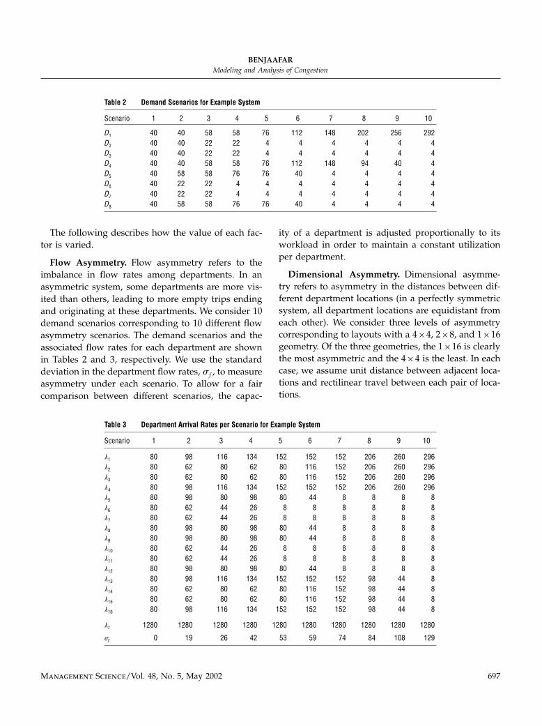
The following describes how the value of each fac-tor is varied.

Flow Asymmetry. Flow asymmetry refers to theimbalance in flow rates among departments. In anasymmetric system, some departments are more vis-ited than others, leading to more empty trips endingand originating at these departments. We consider 10demand scenarios corresponding to 10 different flowasymmetry scenarios. The demand scenarios and theassociated flow rates for each department are shownin Tables 2 and 3, respectively. We use the standarddeviation in the department flow rates, -f , to measureasymmetry under each scenario. To allow for a faircomparison between different scenarios, the capac-

Table 3 Department Arrival Rates per Scenario for Example System

Scenario 1 2 3 4 5 6 7 8 9 10

1 80 98 116 134 152 152 152 206 260 2962 80 62 80 62 80 116 152 206 260 2963 80 62 80 62 80 116 152 206 260 2964 80 98 116 134 152 152 152 206 260 2965 80 98 80 98 80 44 8 8 8 86 80 62 44 26 8 8 8 8 8 87 80 62 44 26 8 8 8 8 8 88 80 98 80 98 80 44 8 8 8 89 80 98 80 98 80 44 8 8 8 810 80 62 44 26 8 8 8 8 8 811 80 62 44 26 8 8 8 8 8 812 80 98 80 98 80 44 8 8 8 813 80 98 116 134 152 152 152 98 44 814 80 62 80 62 80 116 152 98 44 815 80 62 80 62 80 116 152 98 44 816 80 98 116 134 152 152 152 98 44 8

t 1280 1280 1280 1280 1280 1280 1280 1280 1280 1280

�f 0 19 26 42 53 59 74 84 108 129

ity of a department is adjusted proportionally to itsworkload in order to maintain a constant utilizationper department.

Dimensional Asymmetry. Dimensional asymme-try refers to asymmetry in the distances between dif-ferent department locations (in a perfectly symmetricsystem, all department locations are equidistant fromeach other). We consider three levels of asymmetrycorresponding to layouts with a 4×4, 2×8, and 1×16geometry. Of the three geometries, the 1×16 is clearlythe most asymmetric and the 4×4 is the least. In eachcase, we assume unit distance between adjacent loca-tions and rectilinear travel between each pair of loca-tions.



Material-Handling Capacity. For a fixed numberof transporters, material-handling capacity is deter-mined by transporter speed. For each number oftransporters, we consider six values of transporterspeed that correspond to six different levels of trans-porter utilization (under a QAP-optimized layout)ranging from 0.6 to 0.99.

Number of Transporters. We consider systemswith a number of transporters ranging from one tofive. To allow for a fair comparison between systemswith different numbers of transporters, we alwaysmaintain the same overall material-handling capacityby adjusting transporter speed proportionally to thenumber of transporters. This allows us also to distin-guish between the effect of capacity and that of mul-tiplicity of transporters.

Demand and Processing Time Variability. Six lev-els of demand variability are considered by varyingthe squared coefficients of variation of part externalinterarrival times from 0.33 to 2. Similarly, five levelsof processing time variability are considered by vary-ing the squared coefficients of variation of departmentprocessing times from 0.33 to 2.In the following sections, we summarize key results

by describing the effect of each factor on the ratio ,.

Figure 10 The Effect of Flow Asymmetry (4×4 Geometry; nt = 1; Ci = 1 for i = 1� � � � �8; �j = 0�8; Csj= 1 for j = 1� � � � �16; the Series Corresponds

to �t Values of 0.9, 0.95, 98, and 0.989)

0

5

10

15

20

25

30

35

0 20 40 60 80 100 120

σ f

increasing m/h utilization

δ

When appropriate, we also comment on interactionsbetween different factors. For brevity, we show onlya subset of the data we generated. The selected dataare in all cases illustrative of the effects observed inthe larger set.

5.1. The Effect of Flow AsymmetryFirst, let us note that in a symmetric system wheredepartment flow rates are equal, empty travel is lay-out independent since there is equal likelihood of anempty trip originating at any department and endingat any other department. Consequently, the differencein expected WIP between a QAP-optimal and a WIP-optimal layout is always zero. However, a differenceemerges, as we saw in previous sections, when somedepartments are visited more frequently than others.The effect of increasing flow asymmetry on this dif-ference is illustrated in Figure 10.From Figure 10, we see that while the WIP ratio

, is in the neighborhood of one when -f is rela-tively small, it can be significantly higher when -f islarge. Surprisingly, the effect of -f is not monotonic.Although initial increases in -f do lead to a larger ,,additional increases invariably reduce its value. Thus,, is maximum when -f is in the midrange and issignificantly smaller in the extreme cases of either



high or low asymmetry. A possible explanation forthis nonmonotonic behavior is as follows. In a highlyasymmetric system, the demand from one productdominates the demand from all others. Hence, thedepartments that are most visited are those that arevisited by the product with the highest demand.Because these departments are already in neighbor-ing locations under the QAP-optimal layout, the addi-tional reduction in empty travel due to using the WIPcriterion is limited. This is in contrast to situationswhere asymmetry is due to two or more productshaving relatively higher demands than the others. Inthat case, rearranging the layout so that the depart-ments visited by these products are in neighboringlocations does significantly reduce empty travel. Theabove results are summarized in the following obser-vation.Observation 7. The percentage difference in

expected WIP between a QAP-optimal and a WIP-optimal layout is not monotonic in flow asymmetry.It is relatively small for either highly symmetric orasymmetric systems. However, it can be significantwhen flow asymmetry is in the midrange.

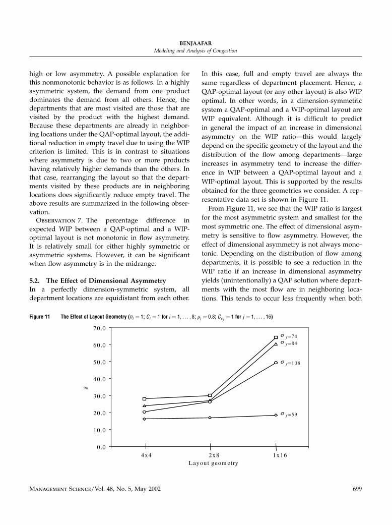
5.2. The Effect of Dimensional AsymmetryIn a perfectly dimension-symmetric system, alldepartment locations are equidistant from each other.

Figure 11 The Effect of Layout Geometry (nt = 1; Ci = 1 for i = 1� � � � �8; �j = 0�8; Csj= 1 for j = 1� � � � �16)

0.0

10 .0

20 .0

30 .0

40 .0

50 .0

60 .0

70 .0

1 2 3 4x4 2x8 1x16 L ayout geom etry

δ

σ f = 59

σ f = 108

σ f = 84

σ f = 74

In this case, full and empty travel are always thesame regardless of department placement. Hence, aQAP-optimal layout (or any other layout) is also WIPoptimal. In other words, in a dimension-symmetricsystem a QAP-optimal and a WIP-optimal layout areWIP equivalent. Although it is difficult to predictin general the impact of an increase in dimensionalasymmetry on the WIP ratio—this would largelydepend on the specific geometry of the layout and thedistribution of the flow among departments—largeincreases in asymmetry tend to increase the differ-ence in WIP between a QAP-optimal layout and aWIP-optimal layout. This is supported by the resultsobtained for the three geometries we consider. A rep-resentative data set is shown in Figure 11.From Figure 11, we see that the WIP ratio is largest

for the most asymmetric system and smallest for themost symmetric one. The effect of dimensional asym-metry is sensitive to flow asymmetry. However, theeffect of dimensional asymmetry is not always mono-tonic. Depending on the distribution of flow amongdepartments, it is possible to see a reduction in theWIP ratio if an increase in dimensional asymmetryyields (unintentionally) a QAP solution where depart-ments with the most flow are in neighboring loca-tions. This tends to occur less frequently when both



Figure 12 The Effect of Material Handling Capacity (�f = 42; 4×4 Geometry; nt = 1; Ci = 1 for i = 1� � � � �8; �j = 0�8; Csj= 1 for j = 1� � � � �16)

0

10

20

30

40

50

3623 3673 3723 3773 3823 3873 3923 3973v

E(WIPt |QAP)

E(WIPt |WIP)

dimensional and flow asymmetry are high. In thesecases, the QAP formulation does not usually favorplacing departments in neighboring locations unlessthey have direct flows between them.Observation 8. The percentage difference in

expected WIP between a QAP-optimal and a WIP-optimal layout is generally increasing in dimensionalasymmetry. In a dimension-symmetric system, a QAP-optimal and aWIP-optimal layout areWIP equivalent.

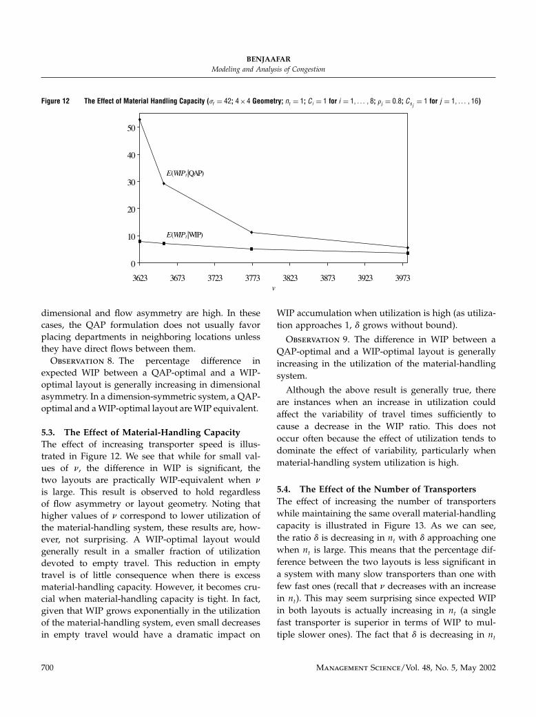
5.3. The Effect of Material-Handling CapacityThe effect of increasing transporter speed is illus-trated in Figure 12. We see that while for small val-ues of ), the difference in WIP is significant, thetwo layouts are practically WIP-equivalent when )

is large. This result is observed to hold regardlessof flow asymmetry or layout geometry. Noting thathigher values of ) correspond to lower utilization ofthe material-handling system, these results are, how-ever, not surprising. A WIP-optimal layout wouldgenerally result in a smaller fraction of utilizationdevoted to empty travel. This reduction in emptytravel is of little consequence when there is excessmaterial-handling capacity. However, it becomes cru-cial when material-handling capacity is tight. In fact,given that WIP grows exponentially in the utilizationof the material-handling system, even small decreasesin empty travel would have a dramatic impact on

WIP accumulation when utilization is high (as utiliza-tion approaches 1, , grows without bound).

Observation 9. The difference in WIP between aQAP-optimal and a WIP-optimal layout is generallyincreasing in the utilization of the material-handlingsystem.

Although the above result is generally true, thereare instances when an increase in utilization couldaffect the variability of travel times sufficiently tocause a decrease in the WIP ratio. This does notoccur often because the effect of utilization tends todominate the effect of variability, particularly whenmaterial-handling system utilization is high.

5.4. The Effect of the Number of TransportersThe effect of increasing the number of transporterswhile maintaining the same overall material-handlingcapacity is illustrated in Figure 13. As we can see,the ratio , is decreasing in nt with , approaching onewhen nt is large. This means that the percentage dif-ference between the two layouts is less significant ina system with many slow transporters than one withfew fast ones (recall that ) decreases with an increasein nt). This may seem surprising since expected WIPin both layouts is actually increasing in nt (a singlefast transporter is superior in terms of WIP to mul-tiple slower ones). The fact that , is decreasing in nt



Figure 13 The Effect of Number of Transporters (�f = 84; 4× 4 Geometry; Ci = 1 for i = 1� � � � �8; �j = 0�8; Csj= 1 for j = 1� � � � �16; the Series

Corresponds to �t Values of 0.95, 98, and 0.989)

0.0

5.0

10.0

15.0

20.0

25.0

30.0

1 3 5 7 9n t

δ increasing m/h utilization

appears to be due mostly to how a change in utiliza-tion affects WIP for different values of nt . For smallvalues of nt a drop in utilization (when it is initiallyhigh) can cause a greater decrease in WIP than the oneseen when nt is large. These results are in line withknown queueing effects in multiserver systems—see,for example, Kleinrock (1976, pp. 279–285). We shouldnote that although the ratio , approaches 1 whennt is large, the difference in WIP can remain signifi-cant. In fact, in many cases we observed the differenceremains relatively constant in nt .

5.5. The Effect of Demand and ProcessingTime Variability

Varying the variability in either demand or process-ing times affects transporter WIP by affecting Cat

. Thiseffect can be gleaned from the expression of Cat

inEquation (26). The value of Cat

is linearly increasing inboth Csi

and Ca0, with the rate of increase an (increas-

ing) function of �t . Hence, we should expect , to beincreasing in both Csi

and Ca0. This is supported by

the numerical results, a sample of which is shown inFigure 14. Note that the effect of process variability ismore pronounced than that of demand, since in ourexperiments process variability is increased uniformlyfor all the departments.

5.6. Managerial ImplicationsTable 4 provides a summary of our results and offersbroad guidelines as to when using WIP as a designcriterion is particularly valuable. The results suggestthat a WIP-optimized layout is most beneficial whenmaterial-handling capacity is limited, dimensionalasymmetry is high, there is asymmetry in the flows,the number of transporters is small, or variabilityin either demand or processing times is high. Theseresults also point to strategies that managers andfacility planners could pursue to increase the robust-ness of layouts with respect to WIP performance—i.e.,investing in excess material-handling capacity, adopt-ing layout geometries that reduce travel distance vari-ance, and ensuring that the most visited processes arecentrally located.Furthermore, these results draw attention to the

importance of indirect interactions that take placebetween different areas of a facility. These indirecteffects have implications for the way we should orga-nize areas of a facility that may otherwise appearindependent. For example, consider a system consist-ing of multiple cells that do not share any productsor processes but are serviced by the same material-handling system. Our results suggest that amongthese cells those that manufacture the products with



Figure 14 The Effect of Demand and Process Variability (�f = 84; 4×4 Geometry; nt = 1, � = 3436, �j = 0�8 for j = 1� � � � �16; the Series Correspondsto Ci Values of 0.35, 1, 1.5, and 2)

21

22

23

24

25

26

27

28

29

30

0.4 0.6 0.8 1.0 1.2 1.4 1.6 1.8 2.0

C Si2

δ

increasing demand variability

the highest demand should be placed in neighbor-ing locations (although they do not share any flows).Our results also show that organizing these cells intoparallel production lines, a common practice in manyfacilities, may lead to greater congestion and longerlead times. Instead, adopting a configuration thatminimizes distance asymmetries (e.g., using a layoutwhere cells are configured into a U-shape and arearranged along a common corridor where most travelwould take place) would maintain the efficient trans-fer of material within cells while freeing up addi-tional material-handling capacity to service the entirefacility.Many companies are beginning to realize the

importance of these indirect effects and are increas-ingly designing layouts that minimize dimensionalasymmetries and reduce empty travel. For exam-ple, GM built its new Cadillac plant in the formof a T to maximize supplier access to the factory

Table 4 When Is Using the WIP Criterion Valuable?

Low Medium High

Flow asymmetry Less valuable More valuable Moderately valuableDimensional asymmetry Less valuable Moderately valuable More valuableMaterial-handling capacity More valuable Moderately valuable Less valuableNumber of transporters More valuable Moderately valuable Less valuableDemand and process variability Less valuable Moderately valuable More valuable

floor and reduce the distance between loading docksand production stocking points (Green 2000). Volvodesigned its Kalmar plant as a collection of hexagon-shaped modules where material flows in concentriclines within each module (Tompkins et al. 1996).Motorola is experimenting with layouts where sharedprocessors are centrally located in functional depart-ments and are equidistant from multiple dedicatedcells within the plant. Variations of the spine lay-out, where departments are placed along the sidesof a common corridor, have been successfully imple-mented in industries ranging from electronic manu-facturing to automotive assembly (Smith et al. 2000,Tanchoco 1994, Tompkins et al. 1996). Layout config-urations that minimize dimensional asymmetries andreduce empty travel are also found in nonmanufactur-ing applications. For example, both the spine and starlayouts are common configurations in airport designs.



Spine and T-shaped layouts are also popular designsfor freight and cross-docking terminals (Gue 1999).

6. Concluding CommentsIn this paper, we showed that minimizing material-handling travel distances does not always reduceWIP. Therefore, the criterion used in the QAP formu-lation of the layout design problem cannot be usedas a reliable predictor of WIP. Because the QAP for-mulation accounts only for full travel, an optimalsolution to the QAP problem tends to favor plac-ing departments that have large intermaterial flowsin neighboring locations. In this paper, we showedthat when we account for empty travel, this may notalways be desirable. Indeed, it can be more benefi-cial if departments that have no direct material flowbetween them are placed in neighboring locations. Inparticular, we found that empty travel can be signif-icantly reduced by placing the most frequently vis-ited departments in neighboring locations regardlessof the amount of flows between these departments.Because WIP is affected by both mean and varianceof travel time, we found that reducing travel-timevariance can be as important as reducing averagetravel time. Equally important, we found that the rel-ative desirability of a layout can be affected by non-material-handling factors, such as department utiliza-tion levels, variability in department processing times,and variability in product demands. We also iden-tified instances where the QAP-and WIP-based for-mulation are WIP equivalent. This includes systemswith flow/dimensional symmetry or systems withlow material-handling system utilization.Several avenues for future research are possible. In

this paper, the objective function was to minimizeoverall WIP in the system. In many applications, itis useful to differentiate between WIP at differentdepartments and/or different stages of the produc-tion process. In fact, in most applications, the value ofWIP tends to appreciate as more work is completedand more value is added to the product. Therefore, itis useful to assign different holding costs for WIP atdifferent stages. This would lead to choosing layoutsthat reduce the most expensive WIP first (e.g., lettingdepartments that participate in the last productionsteps be as centrally located as possible).

In addition to affecting WIP, the choice of layoutdetermines production capacity. From the stabilitycondition, �t < 1, we can obtain the maximum feasiblethroughput rate:

�max�x�= 1/∑

i

∑j

∑k

∑l

∑s

prij �xrkxilxjs�dkl+dls�/)�

(43)

Maximizing throughput by maximizing �max couldbe used as an alternative layout design criterion. Inthis case, layouts would be chosen so that the avail-able material-handling capacity is maximized (i.e., �t

is minimized). The stability condition can also beused to determine the minimum required number ofmaterial-handling devices, nmin, for a given material-handling workload, �t :

nmin = �t

∑i

∑j

∑k

∑l

∑s

prij �xrkxilxjs�dkl+dls�/)� (44)

Minimizing nmin can be used as yet another crite-rion in layout design. More generally, our modelingframework offers the possibility of integrating lay-out design with the design of the material-handlingsystem. For example, we could simultaneously decideon material-handling capacity, such as number orspeed of material-handling devices, and departmentplacement, with the objective of minimizing both WIPholding cost and capital investment costs.In certain applications, there may be a mix of

material-handling technologies. For example, materialtransport between neighboring departments couldbe ensured by continuous conveyors, while materialmovement between more distant departments is car-ried out by a combination of forklift trucks and over-head cranes. In this case, material-handling capac-ity is clearly determined by the mix of technologiesused. It would be useful to examine the relation-ship between layout and the deployment of differentmaterial-handling technology within the same facility.In this paper, we assumed that travel-time variabil-

ity is driven by differences in the distances betweendifferent departments. In some applications, theremight be additional variability due to inherent vari-ability in the travel distance associated with the sametrip or in the speed of travel. Including either typeof variability in computing Expressions (8) and (9)is relatively straightforward. The effect in both cases



would be an increase in Cst. When this type of vari-

ability is high, we should expect the WIP differencebetween the QAP-and the WIP-optimal layouts toincrease.Finally, in our analysis we have assumed that there

is always sufficient capacity for queueing. There aremanufacturing environments where this capacity islimited. Limits on queue sizes can lead to the occa-sional blocking and starvation of the processing depart-ments and the material-handling system, which inturn can reduce system throughput. The analysisof systems with limited queue capacity is consider-ably more complex and is worthy of future research.Although it is not entirely clear how layouts wouldaffect throughput in systems where there is blocking,it is reasonable to conjecture that layouts that reducecongestion by reducing empty and full travel (alongwith variability) would also reduce the probability ofblocking.

AcknowledgmentsThe author would like to thank Wally Hopp, the associate editor,and two anonymous reviewers for many useful comments on anearlier version of the paper. The author is grateful to Te Yang forhelp in generating computer code for the analytical models andcarrying out the simulation experiments. This research is supportedby the National Science Foundation under grant No. DMII-9908437.

ReferencesBenjaafar, S., S. Heragu, S. Irani. 2002. Next generation factory lay-

outs: Research challenges and recent progress. Interfaces Forth-coming.

Bitran, G. R., S. Dasu. 1992. A review of open queueing networkmodels of manufacturing systems. Queueing Systems 12 95–133., D. Tirupati. 1989. Multi-product queueing networks withdeterministic routing: Decomposition approach and the notionof interference. Management Sci. 35 851–878.

Buzacott, J. A., J. G. Shanthikumar. 1993. Stochastic Models of Man-ufacturing Systems. Prentice Hall, Englewood Cliffs, NJ.

Egebelu, P. J. 1987. The use of non-simulation approaches in esti-mating vehicle requirements in an automated guided vehiclebased transport system. Material Flow 4 17–32.

Fu, M. C., B. K. Kaku. 1997a. Minimizing work-in-process andmaterial handling in the facilities layout problem. IIE Trans. 2929–36., . 1997b. On queueing network models and the quadraticassignment problem. Technical report, College of Business andManagement, University of Maryland, College Park, MD.

Green, J. 2000. Why workers are lining up for jobs at this GM plant.Business Week (October 2) �www.businessweek.com�.

Gue, K. 1999. The effect of trailer scheduling on the layout of freightterminals. Transportation Sci. 33 419–428.

Hopp, W., M. L. Spearman. 2000. Factory Physics, 2nd ed.Irwin/McGraw-Hill, New York.

Johnson, M. E., M. L. Brandeau. 1996. Stochastic modeling for auto-mated material handling system design and control. Trans-portation Sci. 30 330–350.

Kraemer, W., M. Langenbach-Belz. 1976. Approximate formulae forthe delay in the queueing system GI/G/1. Congressbook, 8thInternat. Teletraffic Congress, Melbourne, Australia, 235.1–235.8.

Kelton, D. W., R. P. Sadowski, D. A. Sadowski. 1998. Simulation withArena. McGraw-Hill, Boston, MA.

Kleinrock, L. 1976. Queueing Systems, Volume 2: Computer Applica-tions. John Wiley, New York.

Kouvelis, P., A. S. Kiran. 1990. The plant layout problem in auto-mated manufacturing systems. Ann. Oper. Res. 26 397–412., . 1991. Single and multiple period layout modelsfor automated manufacturing systems. Eur. J. Oper. Res. 52300–314.

Meller, R., K. Y. Gau. 1996. The facility layout problem: Recent andemerging trends and perspectives. J. Manufacturing Systems 15351–366.

Pardalos, P. M., H. Wolkowicz. 1994. Quadratic Assignment andRelated Problems. DIMACS Series in Discrete Mathematics,American Mathematical Society, Providence, RI.

Smith, G., J. Wheatley, J. Green. 2000. Car power. Business Week–International Edition (October 23) �www.businessweek.com�.

Solberg, J. J., S. Y. Nof. 1980. Analysis of flow control in alternativemanufacturing configurations. J. Dynamic System MeasurementControl 102 141–147.

Suri, R. 1998. Quick Response Manufacturing: A ComprehensiveApproach to Reducing Lead Times. Productivity Press, Port-land, OR.

Tanchoco, J. M. A. 1994. Material Flow Systems in Manufacturing.Chapman and Hall, London, U.K.

Tompkins, J. A., J. A. White, Y. A. Bozer, E. H. Frazelle, J. M. A. Tan-choco, J. Trevino. 1996. Facilities Planning, 2nd ed. John Wiley,New York.

Whitt, W. 1983a. The queueing network analyzer. Bell System Tech.J. 62 9.

Whitt W. 1983b. Performance of the queueing network analyzer.Bell Systems Tech. J. 63 1911–1979.

Whitt, W. 1993. Approximations for the GI/G/m Queue. ProductionOper. Management 2 114–161.

Womack, J. P., D. T. Jones. 1996. Lean Thinking. Simon and Schuster,New York.

Yang, T., S. Benjaafar. 2001. FLQ: A software for facility layout withqueueing. Technical report—0015, Division of Industrial Engi-neering, Department of Mechanical Engineering, University ofMinnesota, Minneapolis, MN.

Accepted by Wallace J. Hopp; received June 8, 1999. This paper was with the author 17 months for 3 revisions.


Documents

ModelingandAnalysisofCongestion intheDesignofFacilityLayouts · ModelingandAnalysisofCongestion intheDesignofFacilityLayouts ... sign tends to ignore the potential impact of facility