Modeling Unsupervised Perceptual CategoryLearning

Brenden M. Lake, Gautam K. Vallabha, and James L. McClellandDepartment of Psychology, Stanford UniversityJordan Hall Building 420, Stanford, CA 94305

Email: {brenden, mcclelland}@stanford.edu

Abstract—During the learning of speech sounds and otherperceptual categories, category labels are not provided, thenumber of categories is unknown, and the stimuli are encounteredsequentially. These constraints provide a challenge for models,but they have been recently addressed in the Online MixtureEstimation model of unsupervised vowel category learning [1].The model treats categories as Gaussian distributions, proposingboth the number and parameters of the categories. While themodel has been shown to successfully learn vowel categories,it has not been evaluated as a model of the learning process.We account for three results regarding the learning process:infants’ discrimination of speech sounds is better after exposureto a bimodal rather than unimodal distribution [2], infants’discrimination of vowels is affected by acoustic distance [3],and subjects place category centers near frequent stimuli in anunsupervised visual classification task [4].

I. INTRODUCTION

The ability to categorize objects is critical for perception.Knowing an object is in the category “chicken” providescrucial information about that object – such as it has feathers, itis edible, and it can fly. Much modeling work has investigatedhow categories are learned, e.g. [5]–[7].

While category learning is often facilitated by associatingobjects with category labels, categories can be acquired bymere exposure to stimuli – no labels included. For instance,during the first year of life, infants begin acquiring the speechsound categories of their native language; sensitivity to non-native contrasts decreases [8] and sensitivity to native contrastsincreases [9]. In the visual modality, Rosenthal et al. [4] foundthat subjects’ categorical decisions, without feedback, wereinfluenced by the distributional properties of the stimuli.

How can category structure be learned without labels?Models face two challenges: (i) the number of categories tolearn is unknown, and (ii) the stimuli are encountered oneby one in mixed order instead of all at once [1]. Therehas been some recent progress addressing these issues inmodels of speech category learning [1], [10], [11]. The OnlineMixture Estimation (OME) algorithm [1] is an online variantof Expectation-Maximization (EM) that addresses both of theabove issues. It tries to find a set of Gaussian categoriesthat account for a sequence of stimuli, proposing both thenumber and parameters of the categories. The model is alsosomewhat biologically plausible since a topographical networkcan serve as an approximation. In Vallabha et al. [1], the OMEalgorithm successfully learned the number and parameters of

multidimensional vowel categories in English and Japanese[1]. However, successfully learning vowel categories does notimply the algorithm successfully models the learning process.The current work provides such an evaluation.

What quantitative means are available to assess the learningprocess? Category learning is often marked by changes indiscrimination. During the learning process, there is evidencefor improving discrimination across category boundaries (ac-quired distinctiveness) [9], [12], [13] and declining discrim-ination within category boundaries (acquired similarity) [8],[14], terms from [12]. In a very similar algorithm to OMEbut restricted to one dimensional stimuli, McMurray et al.[11] found both effects, defining discrimination as the extentto which two stimuli are members of different estimatedcategories. Should OME show similar effects, it would capturetwo important aspects of the category learning process.

We apply the OME algorithm to three other results regardingthe learning process. The first model is of Maye et al.’s [2]study where infants are sensitized to a [da]-[ta] continuum ofspeech sounds with either a bimodal or unimodal distribution.Infants sensitized to the bimodal distribution showed betterdiscrimination of the endpoints. Second, we investigated howdiscrimination might develop over time. In Sabourin et al.[3], infants showed better discrimination of acoustically moredistinct vowels, and we applied the OME model to this vowelspace. Third, we extended the model from the domain ofspeech to vision, modeling Rosenthal et al.’s [4] unsupervisedcategory learning task where subjects’ categorical choiceswere influenced by the stimulus distribution.

II. THE ONLINE MIXTURE ESTIMATION MODEL

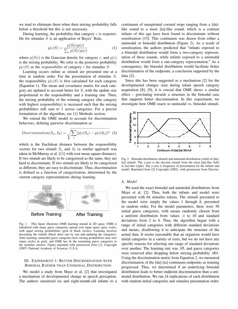
The Online Mixture Estimation (OME) algorithm treats cat-egories as multivariate Gaussians distributions and graduallyestimates the category structure from a sequence of stimuli,proposing both the number of categories and their parameters(Figure 1). The model begins with many (50 or more) initialguess categories distributed randomly about the space in whichthe data reside.1 Each guess category has an associated mixingprobability, the probability of the guess category contributinga random token to the stimulus set. In our simulations, allguess categories were initialized to be equally likely. For speed

1In our simulations, the initial guess category covariance matrices werediagonal (although the full covariance matrix is updated during learning).The initial variances along the diagonal were random.

we tend to eliminate them when their mixing probability fallsbelow a threshold but this is not necessary.

During learning, the probability that category c is responsi-ble for stimulus S is an application of Bayes’ Rule,

p(c|S) =p(S|c)p(c)∑c p(S|c)p(c)

(1)

where p(S|c) is the Gaussian density for category c, and p(c)is the mixing probability. We refer to the posterior probabilityp(c|S) as the responsibility of category c for stimulus S.

Learning occurs online as stimuli are presented one at atime in random order. For the presentation of stimulus S,the responsibility p(c|S) is first calculated for each category(Equation 1). The mean and covariance matrix for each cate-gory are updated to account better for S, with the update sizeproportional to the responsibility and a learning rate. Then,the mixing probability of the winning category (the categorywith highest responsibility) is increased such that the mixingprobabilities still sum to 1 across categories. For a preciseformulation of the algorithm, see [1] Methods section.

We extend the OME model to account for discriminationbehaviors, defining pairwise discrimination as

Discrimination(Sa, Sb) =√∑

c

(p(c|Sa)− p(c|Sb))2 (2)

which is the Euclidean distance between the responsibilityvectors for two stimuli Sa and Sb (a similar approach wastaken in McMurray et al. [11] with root mean square distance).If two stimuli are likely to be categorized as the same, they arehard to discriminate. If two stimuli are likely to be categorizedas different, they are easy to discriminate. Thus, discriminationis defined as a function of categorization, determined by thecurrent category representations during learning.

Fig. 1. This figure illustrates OME learning stimuli in 2D space. OME isinitialized with many guess categories spread over input space (grey ovals),with equal mixing probabilities (grid of black circles). Learning involvespresenting the stimuli (black dots) one by one and updating the categories.After learning, unneeded guess categories have mixing probabilities near zero(open circles in grid), and OME has fit the remaining guess categories tothe stimulus clusters. Figure reprinted with permission from [1], Copyright(2007) National Academy of Sciences, U.S.A.

III. EXPERIMENT 1: BETTER DISCRIMINATION WITHBIMODAL RATHER THAN UNIMODAL DISTRIBUTION

We model a study from Maye et al. [2] that investigateda mechanism of developmental change in speech perception.The authors sensitized six and eight-month-old infants to a

continuum of unaspirated coronal stops ranging from a [da]-like sound to a more [ta]-like sound, which is a contrastinfants of this age have been found to discriminate withoutsensitization [15]. This continuum was drawn from either aunimodal or bimodal distribution (Figure 2). As a result ofsensitization, the authors predicted that “infants exposed toa bimodal distribution would form a two-category represen-tation of these sounds, while infants exposed to a unimodaldistribution would form a one-category representation.” As aconsequence, the bimodal distribution would facilitate betterdiscrimination of the endpoints, a conclusion supported by thedata [2].

Since this has been suggested as a mechanism [2] for thedevelopmental changes seen during infant speech categoryacquisition [8], [9], it is crucial that OME shows a similareffect – gravitating towards a structure in the bimodal casethat supports better discrimination. In this experiment, weinvestigate how OME reacts to unimodal vs. bimodal stimuli.

Fig. 2. Bimodal distribution (dotted) and unimodal distribution (solid) of [da]-[ta] stimuli. The x-axis is the discrete stimuli from the most [da]-like (left)to [ta]-like (right). The y-axis is frequency of presentation for the infants andmodel. Reprinted from [2] Copyright (2002), with permission from Elsevier.

A. Model

We used the exact bimodal and unimodal distributions fromMaye et al. [2]. Thus, both the infants and model werepresented with 64 stimulus tokens. The stimuli presented tothe model were simply the values 1 through 8, presentedin random order. For the model parameters, there were 50initial guess categories, with means randomly chosen froma uniform distribution from values -1 to 10 and standarddeviations from 2 to 4. Thus, the algorithm began with arange of initial categories with different standard deviationsand means, disallowing it to anticipate the structure of theactual data. It seems reasonable that an organism would haveinitial categories in a variety of sizes, but we do not have anyspecific reasons for selecting one range of standard deviationsover another. The learning rate was .05, and guess categorieswere removed after dropping below mixing probability .001.Using the discrimination metric from Equation 2, we measureddiscrimination of the [da]-[ta] continuum endpoints as trainingprogressed. Thus, we determined if an underlying bimodaldistribution leads to better endpoint discrimination than a uni-modal distribution. We ran 24 replications of each distributionwith random initial categories and stimulus presentation order.

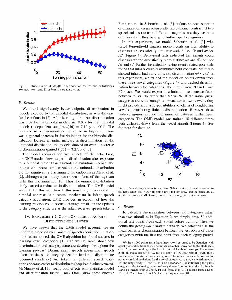
Fig. 3. Time course of [da]-[ta] discrimination for the two distributionsaveraged over runs. Error bars are standard error.

B. Results

We found significantly better endpoint discrimination inmodels exposed to the bimodal distribution, as was the casefor the infants in [2]. After learning, the mean discriminationwas 1.02 for the bimodal models and 0.079 for the unimodalmodels (independent samples t(46) = 7.12, p < .001). Thetime course of discrimination is plotted in Figure 3. Therewas a general increase in discrimination for the bimodal dis-tribution. Despite an initial increase in discrimination for theunimodal distribution, the models showed an overall decreasein discrimination (paired t(23) = 3.27, p < .01).

The model accounts for two aspects of the data. First,the OME model shows superior discrimination after exposureto a bimodal rather than unimodal distribution. Second, theinfants who were familiarized to the unimodal distributiondid not significantly discriminate the endpoints in Maye et al.[2], although a past study has shown infants of this age canmake this discrimination [15]. Thus, the unimodal distributionlikely caused a reduction in discrimination. The OME modelaccounts for this reduction. If this sensitivity to unimodal vs.bimodal contrasts is a central mechanism in infant speechcategory acquisition, OME provides an account of how thelearning process could occur – through small, online updatesto the category structure as the infant receives speech tokens.

IV. EXPERIMENT 2: CLOSE CATEGORIES ACQUIREDISTINCTIVENESS SLOWER

We have shown that the OME model accounts for animportant proposed mechanism of speech acquisition. Further-more, as mentioned, the OME algorithm has found success inlearning vowel categories [1]. Can we say more about howdiscrimination and category structure develops throughout thelearning process? During infant speech acquisition, speechtokens in the same category become harder to discriminate(acquired similarity) and tokens in different speech cate-gories become easier to discriminate (acquired distinctiveness).McMurray et al. [11] found both effects with a similar modeland discrimination metric. Does OME show these effects?

Furthermore, in Sabourin et al. [3], infants showed superiordiscrimination on an acoustically more distinct contrast. If twospeech tokens are from different categories, are they easier todiscriminate if they belong to further apart categories?

In this experiment, we model Sabourin et al. [3] whotested 8-month-old English monolinguals on their ability todiscriminate acoustically similar vowels /e/ vs. /I/ and /e/ vs./E/ (Figure 4). Behavioral tests indicated that infants coulddiscriminate the acoustically more distinct /e/ and /E/ but not/e/ and /I/. Further investigation using event-related potentialsfound that infants could discriminate both contrasts, but it alsoshowed infants had more difficulty discriminating /e/ vs. /I/. Inthis experiment, we trained the model on points drawn fromthese three vowel categories (Figure 4), and tracked discrimi-nation between the categories. The stimuli were 2D in F1 andF2 space. We would expect discrimination to increase fasterbetween /e/ vs. /E/ rather than /e/ vs. /I/. If the initial guesscategories are wide enough to spread across two vowels, theymight provide similar responsibilities to tokens of neighboringvowels, contributing little to discrimination. However, thesewide categories may aid discrimination between further apartcategories. The OME model was trained 10 different timeswith different draws from the vowel stimuli (Figure 4). Seefootnote for details.2

Fig. 4. Vowel categories estimated from Sabourin et al. [3] and converted tothe Bark scale. The 1000 blue points are a random draw, and the black circlesare the categories OME found, plotted 1 s.d. along each principal axis.

A. Results

To calculate discrimination between two categories ratherthan two stimuli as in Equation 2, we simply drew 50 addi-tional test points from each vowel before training. Then wedefine the perceptual distance between two categories as themean pairwise discrimination between the test points of thosecategories (with the first test point from each category paired,

2We drew 1000 points from these three vowel, assumed to be Gaussian, withequal probability from each. The points were then converted to the Bark scale(1 to 24, corresponding to the first 24 critical bands of hearing). There were50 initial guess categories. We ran the algorithm 10 times with different drawsfor the vowel points and initial categories. The authors provide the means butnot the standard deviations for the vowel categories, so they were estimated as1/3 the range along F1 and F2 with no covariance. For initializing the guesscategories, the following were randomly drawn from uniform distributions inBark: F1 means from 3.9 to 8, F1 s.d. from .5 to 1, F2 means from 12.4 to15, and F2 s.d. from .5 to 1.5. The learning rate was .01.

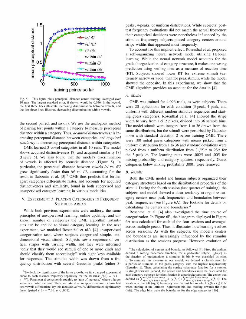
Fig. 5. This figure plots perceptual distance across training, averaged over10 runs. The largest standard error, if shown, would be 0.036. In the legend,the first three lines illustrate increasing discrimination between vowels, andthe last three lines illustrate decreasing discrimination within vowels.

the second paired, and so on). We use the analogous methodof pairing test points within a category to measure perceptualdistance within a category. Thus, acquired distinctiveness is in-creasing perceptual distance between categories, and acquiredsimilarity is decreasing perceptual distance within categories.

OME learned 3 vowel categories in all 10 runs. The modelshows acquired distinctiveness [9] and acquired similarity [8](Figure 5). We also found that the model’s discriminationof vowels is affected by acoustic distance (Figure 5). Inparticular, the perceptual distance between vowels /e/ vs. /E/grew significantly faster than /e/ vs. /I/, accounting for theresult in Sabourin et al. [3].3 OME thus predicts that furtherapart categories differentiate faster, and accounts for acquireddistinctiveness and similarity, found in both supervised andunsupervised category learning in various modalities.

V. EXPERIMENT 3: PLACING CATEGORIES IN FREQUENTSTIMULUS AREAS

While both previous experiments were auditory, the sameprinciples of unsupervised learning, online updating, and un-known number of categories the OME algorithm instanti-ates can be applied to visual category learning. In the nextexperiment, we modeled Rosenthal et al.’s [4] unsupervisedcategorization task, where subjects categorized simple, one-dimensional visual stimuli. Subjects saw a sequence of ver-tical stripes with varying width, and they were informed“only that they would see stimuli of one or more kinds andshould classify them accordingly,” with eight keys availablefor responses. The stimulus width was drawn from a fre-quency distribution with several Gaussian peaks (either 3-

3To check the significance of the faster growth, we fit a damped exponentialcurve to each distance trajectory separately for the 10 runs: f(x) = c(1 −e−dx). Parameter d corresponds roughly to “rate of increase,” where a largervalue is a faster increase. Thus, we take d as an approximation for how fasttwo vowels differentiate. By this measure, /e/ vs. /E/ differentiates significantlyfaster (paired t(9) = 7.39, p < .001).

peaks, 4-peaks, or uniform distribution). While subjects’ post-test frequency evaluations did not match the actual frequency,their categorical decisions were nonetheless influenced by thestimulus frequency; subjects placed category centers aroundstripe widths that appeared most frequently.

To account for this implicit effect, Rosenthal et al. proposeda self-organizing neural network model utilizing Hebbianlearning. While the neural network model accounts for thegradual organization of category structure, it makes one wrongprediction using settling time as a measure of reaction time(RT). Subjects showed lower RT for extreme stimuli (ex-tremely narrow or wide) than for peak stimuli, while the modelshowed the opposite. In this experiment, we show that theOME algorithm provides an account for the data in [4].

A. Model

OME was trained for 4,096 trials, as were subjects. Therewere 20 replications for each condition (3-peak, 4-peak, anduniform) with different random stimulus sequences and start-ing guess categories. Rosenthal et al. [4] allowed the stripewidth to vary from 1-512 pixels, divided into 36 sample bins.The model stimuli were integers from 1 to 36 drawn from thesame distributions, but the stimuli were perturbed by Gaussiannoise with standard deviation 2 before training OME. Therewere 100 initial guess categories with means picked from auniform distribution from 1 to 36 and standard deviations werepicked from a uniform distribution from (1/2)σ to 25σ forthe 3-peak σ. The learning rates were .0025 and .005 formixing probability and category updates, respectively. Guesscategories below mixing probability .0001 were removed.

B. Results

Both the OME model and human subjects organized theircategory structures based on the distributional properties of thestimuli. During the fourth session (last quarter of training), thesubjects and model showed a clear tendency to organize cat-egory centers near peak frequencies and boundaries betweenpeak frequencies (see Figure 6A). See footnote for details oncalculating the centers and boundaries.4

Rosenthal et al. [4] also investigated the time course ofcategorization. In Figure 6B, the histogram displayed in Figure6A was calculated for each of the four sessions and averagedacross multiple peaks. Thus, it illustrates how learning evolvesacross sessions. As with the subjects, the model’s centersand boundaries are increasingly influenced by the stimulusdistribution as the sessions progress. However, evolution of

4The calculation of centers and boundaries followed [4]. First, the authorsdefined a sorting coherence function, for a particular subject, χ(b, c) asthe fraction of presentations a stimulus in bin b was classified as classc. To simulate this measure in our model, we defined a classification fora particular stimulus as the guess category with the highest responsibility(Equation 1). Then, calculating the sorting coherence function for a sessionis straightforward. Second, the center and boundaries must be calculated foreach category c chosen for classification in a particular session. The center wasdefined as

∑right boundary

b=left boundaryb · χ(b, c)/

∑right boundary

b=left boundaryχ(b, c). The

location of the left (right) boundary was the last bin in which χ(b, c) ≤ 0.5,when starting at the leftmost (rightmost) bin and moving towards the right(left). The edge bins were the boundaries for the edge categories [16].

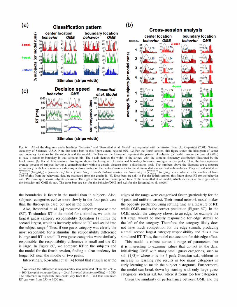
Fig. 6. All of the diagrams under headings “behavior” and “Rosenthal et al. Model” are reprinted with permission from [4], Copyright (2001) NationalAcademy of Sciences, U.S.A. Note that some bars in this figure extend beyond 60%. (a) For the fourth session, this figure shows the histogram of centerand boundary locations for the subjects and the model. The bars on the histogram represent the percent of subjects (or model runs in the case of OME)to have a center or boundary in that stimulus bin. The x-axis denotes the width of the stripes, with the stimulus frequency distribution illustrated by theblack curve. (b) For all four sessions, this figure shows the histogram of center and boundary locations, averaged across peaks. Thus, the bars representaverage percent of subjects having a center/boundary within a certain distance from a distribution peak. The numbers above the diagrams are a measureof accuracy, with lower numbers indicating a closer match of the centers/boundaries to the stimulus distribution centers/boundaries. They are calculated as:∑nbars

k=1(heightk) ∗ (number of bars from bark to distribution center [or boundary])/

∑nbars

k=1heightk where nbars is the number of bars.

The heights from the behavioral data are estimated from the graphs in [4]. Error bars are s.d. (c) For the fourth session, this figure shows RT for the behaviorand OME, averaged across subjects (or runs). The right column shows convergence time of the Rosenthal et al. model, which increases at the edges wherethe behavior and OME do not. The error bars are s.e. for the behavior/OME and s.d. for the Rosenthal et al. model.

the boundaries is faster in the model than in subjects. Also,subjects’ categories evolve more slowly in the four-peak casethan the three-peak case, but not in the model.

Also, Rosenthal et al. [4] measured subject response time(RT). To simulate RT in the model for a stimulus, we took thelargest guess category responsibility (Equation 1) minus thesecond largest, which is inversely related to RT and scaled intothe subject range.5 Thus, if one guess category was clearly themost responsible for a stimulus, the responsibility differenceis large and RT is small. If two guess categories were similarlyresponsible, the responsibility difference is small and the RTis large. In Figure 6C, we compare RT in the subjects andthe model for the fourth session, finding a clear tendency forlonger RT near the middle of two peaks.

Interestingly, Rosenthal et al. [4] found that stimuli near the

5We scaled the difference in responsibility into simulated RT in ms: RT =−400(Largest responsibility− 2nd Largest Responsibility) + 1050.The difference in responsibilities could vary from 0 to 1, and thus simulatedRT can vary from 650 to 1050 ms.

edges of the range were categorized faster (particularly for the4-peak and uniform cases). Their neural network model makesthe opposite prediction using settling time as a measure of RT,while OME makes the correct prediction (Figure 6C). In theOME model, the category closest to an edge, for example theleft edge, would be mostly responsible for edge stimuli tothe left of the category. Therefore, the category likely doesnot have much competition for the edge stimuli, producinga small second largest category responsibility and thus a lowsimulated RT. Thus, the model can account for this edge effect.

This model is robust across a range of parameters, butit is interesting to examine values that do not fit the data.Initializing OME with many small guess categories, such ass.d. (1/2)σ where σ is the 3-peak Gaussian s.d., without anincrease in learning rate results in too many categories inearly learning to match the subject histograms. Furthermore,the model can break down by starting with only large guesscategories, such as s.d. 6σ, where it forms too few categories.

Given the similarity of performance between OME and the

behavior, OME is a particularly good model of unsupervisedcategorization when stimuli are drawn from a Gaussian mix-ture. As with the subjects, the inferred center and boundarylocations were influenced by the distribution frequencies, withthe influence evolving over training time. Furthermore, as withthe subjects, it seems natural that OME would be more certainabout a categorization query for peak and edge stimuli.

VI. GENERAL DISCUSSION

Categorization is essential to perception, and much of cate-gory learning is unsupervised. How can category structure belearned from just a sequence of stimuli? The Online MixtureEstimation (OME) algorithm [1] has provided some progress,showing that the number and parameters of vowel categoriescan be learned through online updating. However, showing thealgorithm can solve the required learning problem [1] does notshow the algorithm is a model of the processes to get there.

From this work, there are several results to recommendOME as a process model of category learning. In Experiment1, the model produced better discrimination after exposure toa bimodal rather than unimodal distribution, accounting fora proposed mechanism of infant speech acquisition [2]. Toinvestigate how discrimination develops over time, in Experi-ment 2, the OME model was applied to a crowded vowel space[3]. Both infants and the model showed better discriminationof a more acoustically dissimilar contrast than a more similarcontrast. Also in Experiment 2, discrimination between vowelsincreased over time (acquired distinctiveness) and discrimina-tion within vowels decreased over time (acquired similarity);both effects have empirical evidence from various modalities[8], [9], [12]–[14] and follow naturally from the modelingframework. In Experiment 3, the OME model showed thatthe same principles governing auditory category learning canbe applied to visual category learning, where both subjectand model categorization choices and response times wereinfluenced by the distribution of stimuli. As previously noted,the model does not yet match some aspects of the humantime-evolution data, an issue we are currently investigating.

More generally, OME provides an elegant solution to theproblems of (1) scalability, (2) sensitivity, (3) revisability, and(4) cross-modal fusion in category learning. (1) Regardingscalability, OME’s computational complexity is largely inde-pendent of the number of functionally useful data categories,only influencing complexity by affecting the number of guesscategories. (2) Also, OME is sensitive to overlapping cat-egories, reconstructing the data distribution from categorieswith means as close as 2.5 s.d. apart. (3) Additionally, themodel is able to revise its solution if presented dynamic datacategories. If a data category is removed from presentation,OME’s corresponding guess category will progressively dropin mixing probability. If a new data category is added duringlearning and unused guess categories are not removed, they canprovide a mechanism for adding categories. (4) Furthermore,OME can learn cross-modal categories. Combining auditoryand visual dimensions, such as speech and the speaker’s mouthposition, is entirely compatible with the approach.

There is much to explore in future work, including howrepeated stimulation affects sensitivity. In Jenkins et al. [17],monkeys placed their fingers in contact with a rotating diskin exchange for reward many times a day over months. Thisrepeated stimulation of the fingertips resulted in shrinkage ofreceptive fields and expanded cortical area for the stimulatedsurface, likely improving sensitivity in this region. In contrast,repeated and concentrated stimulation in OME would likelyform a category, resulting in decreased sensitivity due toacquired similarity. The issue here is empirical as well astheoretical; it is not yet clear why some experiments pro-duce increased sensitivity, while others produce decreasedsensitivity, to clustered stimul. We are examining whethermodifications to OME could produce the opposite behavior,potentially providing insight into this deep question.

REFERENCES

[1] G. K. Vallabha, J. L. McClelland, F. Pons, J. F. Werker, andS. Amano, “Unsupervised learning of vowel categories from infant-directed speech,” Proceedings of the National Academy of Science, vol.104, no. 33, pp. 13 273–13 278, 2007.

[2] J. Maye, J. F. Werker, and L. Gerken, “Infant sensitivity to distributionalinformation can affect phonetic discrimination,” Cognition, vol. 82, pp.B101–B111, 2002.

[3] L. Sabourin, J. F. Werker, L. Bosch, and N. Sebastian-Galles, “Perceivingvowels in a tight vowel space: evidence from monolingual infants,”Developmental Science, under revision.

[4] O. Rosenthal, S. Fusi, and S. Hochstein, “Forming classes by stimulusfrequency: behavior and theory,” Proceedings of the National Academyof Science, vol. 98, pp. 4265–4270, 2001.

[5] T. T. Rogers and J. L. McClelland, Semantic Cognition: A ParallelDistributed Processing Approach. Cambridge, MA: MIT Press, 2004.

[6] J. R. Anderson, “The adaptive nature of human categorization,” Psycho-logical Review, vol. 98, pp. 409–429, 1991.

[7] T. L. Griffiths, A. N. Sanborn, K. R. Canini, and D. J. Navarro,“Categorization as nonparametric bayesian density estimation,” in Theprobabilistic mind: Prospects for rational models of cognition, M. Oaks-ford and N. Chater, Eds. Oxford: Oxford University Press, 2008.

[8] J. F. Werker and R. C. Tees, “Cross-language speech perception:evidence for perceptual reorganization during the first year of life,” InfantBehavior and Development, vol. 7, pp. 49–63, 1984.

[9] P. K. Kuhl, E. Stevens, A. Hayashi, T. Deguchi, S. Kiritani, andP. Iverson, “Infants show a facilitation effect for native language phoneticperception between 6 and 12 months,” Developmental Science, vol. 9,no. 2, pp. F13–F21, 2006.

[10] B. de Boer and P. K. Kuhl, “Investigating the role of infant-directedspeech with a computer model,” Acoustics Research Letters Online,vol. 4, pp. 129–134, 2003.

[11] B. McMurray, R. N. Aslin, and J. Toscano, “Statistical learning ofphonetic categories: Insights from a computational approach,” Devel-opmental Science, in press.

[12] R. K. Goldstone, “Influences of categorization on perceptual discrimi-nation,” Journal of Experimental Psychology: General, vol. 123, no. 2,pp. 178–200, 1994.

[13] S. V. Stevenage, “Which twin are you? a demonstration of inducedcategorical perception of identical twin faces,” British Journal of Psy-chology, vol. 89, pp. 39–57, 1998.

[14] K. R. Livingston, J. K. Andrews, and S. Harnad, “Categorical perceptioneffects induced by category learning,” Journal of Experimental Psychol-ogy, vol. 24, no. 3, pp. 732–753, 1998.

[15] J. E. Pegg and J. F. Werker, “Adult and infant perception of two englishphones,” Journal of the Acoustical Society of America, vol. 102, pp.3742–3753, 1997.

[16] O. Rosenthal, Personal Communication, January 2008.[17] W. M. Jenkins, M. M. Merzenich, M. T. Ochs, T. Allard, and E. Guıc-

Robles, “Functional reorganization of primary somatosensory cortex inadult owl monkeys after behaviorally controlled tactile stimulation,”Journal of Neurophysiology, vol. 63, no. 1, pp. 82–104, 1990.