Modeling the Within-Host Dynamics of Cholera:Bacterial-Viral Interaction

Xueying Wang a,∗ and Jin Wang b

a Department of Mathematics,Washington State University, Pullman, WA 99164, USA

∗ Email: xueying@math.wsu.edu

b Department of Mathematics,University of Tennessee at Chattanooga, Chattanooga, TN 37403

Email: jin-wang02@utc.edu

Abstract

Novel deterministic and stochastic models are proposed in this paper for thewithin-host dynamics of cholera, with a focus on the bacterial-viral interaction. Thedeterministic model is a system of differential equations describing the interactionamong the two types of vibrios and the viruses. The stochastic model is a systemof Markov jump processes that is derived based on the dynamics of the determin-istic model. The multitype branching process approximation is applied to estimatethe extinction probability of bacteria and viruses within a human host during theearly stage of the bacterial-viral infection. Accordingly, a closed-form expression isderived for the disease extinction probability, and analytic estimates are validatedwith numerical simulations. The local and global dynamics of the bacterial-viralinteraction are analyzed using the deterministic model, and the result indicates thatthere is a sharp disease threshold characterized by the basic reproduction numberR0: if R0 < 1, vibrios ingested from the environment into human body will notcause cholera infection; if R0 > 1, vibrios will grow with increased toxicity and per-sist within the host, leading to human cholera. In contrast, the stochastic modelindicates, more realistically, that there is always a positive probability of diseaseextinction within the human host.

1 Introduction

Cholera, an ancient disease, has re-emerged as a major health threat to developing countriesand caused several major outbreaks in recent years, including those in Haiti from 2010 to2012 and in Zimbabwe from 2008 to 2009, with wide-spread infections and high morbidity(and, in some cases, mortality) levels. Cholera is caused by the bacterium vibrio cholerae;it can be transmitted from the environment to people ingesting the contaminated water,or between human hosts through direct/indirect contact with infected individuals (e.g.,hugging, shaking hands, and eating food prepared by dirty hands).

1

Many mathematical epidemiological models have been published to investigate thetransmission dynamics of cholera at the between-host level; see, e.g., [5,6,11,16,17,19–21,24,27,29]. These models generally incorporate an environmental pathogen component (typ-ically, the concentration of the vibrios) into a SIR (susceptible-infected-recovered) epidemicframework. Some of these models only considered the environment-to-human transmissionroute (e.g., [11,17]), whereas other models have included both the environment-to-humanand human-to-human transmission pathways (e.g., [16, 20, 21, 24]). Models involving gen-eral incidence and environmental pathogen representations have also been proposed andanalyzed [19,22,23,26,31,32].

In contrast to the large number of between-host cholera models, very little effort hasbeen devoted to the within-host dynamics of cholera, partly due to the complication ofthe biochemical and genetic interactions that occur within the human body. Recently, acoupled between-host and within-host cholera model was proposed [28], but the within-host dynamics in that work take a very simple form, represented by one single equationcharacterizing the increased toxicity of the vibrios inside the human body.

When the vibrios are ingested from the environment and reach the small intestinewithin the human body, complex biological interaction, chemical reaction, and genetictransduction take place that lead to human cholera [7,9]. Among these the bacterial-viralinteraction is of key importance. The virus (typically, the cholera-toxin phage) plays acritical role in the pathogenesis of the vibrios. Such a virus attaches itself to the surface ofthe bacteria and inject its DNA into the bacterial cells, causing lateral gene transfer of thevibrios and forming cholera toxin, the major virulence factor of cholera. The transducedvibrios have an infectivity much higher (up to 700-fold) than the original vibrios ingestedfrom the environment [18]. These highly toxic vibrios then cause human cholera symptoms,most commonly seen as severe diarrhea. Subsequently, these vibrios are shed out of humanbody, but they remain at the highly infectious state for several hours, during which timethey can be transmitted to other human hosts.

To make a distinction between the two types of vibrios involved in this study, we usethe term ‘environmental vibrios’ to refer to those bacteria originated from the environmentwhich usually have a low infectivity, and ‘human vibrios’ for those bacteria generated withinthe human body, typically through the interaction between the virus and the ingestedenvironmental vibrios, which have a much higher infectivity.

The present paper aims to mathematically model and understand the within-host dy-namics of cholera. To that end, we first construct a deterministic differential equationsystem to investigate the interaction between the environmental and human vibrios andthe virus. We conduct careful equilibrium analysis on this model, with a focus on thedisease threshold dynamics. The deterministic model, however, may not reflect the realitywell in cases where the bacterial and viral population sizes are not sufficiently large andwhere the randomness plays a role. Thus, we also propose and analyze a stochastic Markovjump process model to complement the deterministic dynamics. In particular, we estimatethe probability of disease extinction from our stochastic model using the branching process

2

approximations.We organize the remainder of the paper as follows. In Section 2, we present the deter-

ministic model, analyze the equilibria, and conduct both local and global stability analysis.In Section 3, we construct the stochastic model and derive the disease extinction probabil-ity. In Section 4, we conduct numerical simulation of both models and compare the results;we also numerically verify the disease extinction probability based on the stochastic model.Finally, we conclude the paper in Section 5 with some discussion.

2 Deterministic Model

2.1 Model Formulation

We consider the bacterial-viral interaction taking place in the small intestine, where thevibrios initially enter the human body from the contaminated environment by ingestion.Through the interaction with the virus (phage), the environmental vibrios are transformedinto highly toxic human vibrios by phage transduction. We assume that the bacterial-viralinteraction is subject to saturation in terms of the environmental vibrios. Our deterministicmodel representing the within-host cholera dynamics is formulated as the following systemof ordinary differential equations:

dB

dt= Λ− α B

κ+BV − δ1B,

dZ

dt= g(Z) + θ1 α

B

κ+BV − δ2Z,

dV

dt=h(V ) + θ2 α

B

κ+BV − δ3V.

(2.1)

Here B and Z represent the concentrations of the environmental vibrios and human vibrios,respectively, and V refers to the concentration of the virus. Λ is the influx rate of theingested environmental vibrios, α is the contact rate between the environmental vibriosand the virus. δi (i = 1, 2, 3) denotes the per capita death rate of each compartment.θ1 and θ2 are rescaled coefficients that capture the generation rates of Z and V throughbacterial-viral interactions, respectively. Meanwhile, we introduce two functions g(Z) andh(V ) to account for the intrinsic growth of Z and V , respectively, in the course of thebiochemical and genomic interactions.

We note that the intrinsic growth of microorganisms inside the human body may dependon several factors of the host such as the health condition and the immunity level, andmay vary for different individuals. Thus, we intend to keep these functions as general aspossible, subject to a few biologically feasible conditions. Specifically, we assume:

(H1) (a) g(0) = 0; (b) g′(Zg) < δ2 for some Zg ≥ 0; (c) g′′(Z) ≤ 0;

(H2) (a) h(0) = 0; (b) h′(Vh) < δ3 for some Vh ≥ 0; (c) h′′(V ) ≤ 0.

3

The assumptions (H1) and (H2) state that the intrinsic growth is subject to saturationand when the bacterial/viral concentration is sufficiently high, the intrinsic growth will beoutcompeted by the natural death/removal. We also note that in most cases, h(v) = 0could be used in the representation of viral dynamics, though we intend to treat it as aspecial case of our general formulation.

2.2 Analysis of the Deterministic Model

2.2.1 The Basic Reproduction Number

An important disease threshold is the basic reproduction number R0 [3]. It is apparent thatthe model (2.1) always admits the invasion-free equilibrium (IFE), (B,Z, V ) = (B0, 0, 0),for which B0 = Λ/δ1. Furthermore, the disease components in this model are Z and V ,and the new infection matrix F and the transition matrix V are

F =

[gZ θ1 αB0/(B0 + κ)0 hV + θ2 αB0/(B0 + κ)

], (2.2)

and

V =

[δ2 00 δ3

], (2.3)

wheregZ = g′(0), hV = h′(0). (2.4)

By the next generation matrix method [25], the basic reproduction number is defined asthe spectral radius of the next generation matrix K = FV−1; i.e.,

R0 = ρ(K) = maxR0Z , R0V

, (2.5)

where

R0Z =gZδ2, and R0V =

hVδ3

+θ2αB0

δ3(B0 + κ).

The terms R0Z and R0V , respectively, correspond to the expected numbers of secondaryinfections caused by one human vibrio and one virus during its lifetime in the human host.The basic reproduction number R0 here denotes the average number of secondary infectionsproduced by one infectious microorganism over the course of its infectious period in anotherwise uninfected population. The expression (2.5) shows that R0 is the maximumof R0V and R0Z , indicating that the within-host cholera infection risk depends on thedynamics of both the human vibrios and the viruses.

4

2.2.2 Equilibrium Analysis

In this section, we will study the nontrivial equilibrium solution, X∗ = (B∗, Z∗, V ∗), ofmodel (2.1), where by a nontrivial equilibrium, we mean an equilibrium that is not theIFE. Its components must satisfy

Λ− α B∗

κ+B∗V ∗ − δ1B∗ = 0,

g(Z∗) + θ1 αB∗

κ+B∗V ∗ − δ2Z∗ = 0,

h(V ∗) + θ2 αB∗

κ+B∗V ∗ − δ3V ∗ = 0.

(2.6)

Solving (2.6) yields

B∗ =1

δ1

(Λ− δ2Z

∗ − g(Z∗)

θ1

),

B∗ = φ(V ∗),

V ∗ = ψ(B∗),

(2.7)

with

φ(V ) :=1

δ1

(Λ− δ3V − h(V )

θ2

),

ψ(B) :=(Λ− δ1B)(κ+B)

αB.

(2.8)

First, let’s consider the intersection of the graphs B = φ(V ) and V = ψ(B) on V -B

plane. Note that ψ′(B) = −Λκ+B2δ1αB2

< 0, ψ′′(B) =2Λκ

αB3> 0, φ′(V ) =

h′(V )− δ3δ1θ2

and

φ′′(V ) =h′′(V )

δ1θ2. By assumption (H2), φ′(V ) < 0 for V ≥ Vh and φ′′(V ) ≤ 0. Hence,

B = φ(V ) is always concave down and strictly decreasing when V is sufficiently large,whereas V = ψ(B) is strictly decreasing and concave up. Meanwhile, we notice thatthese two curves have a unique intersection (V, B) = (0, B0) on the boundary of R+

2 andlimB→0+ ψ(B) =∞. This implies that these graphs admit at most two intersections in R+

2 .Furthermore, the existence of the intersection (Ve, Be) in the interior of R+

2 depends on theslopes of these curves at (V, B) = (0, B0). Specifically, these two graphs intersect in theinterior of R+

2 ⇐⇒ φ′(0) > ψ′(B0)−1 (see Figure 1). One can verify by direct calculation

that

φ′(0) > ψ′(B0)−1 ⇐⇒ R0V =

hV + θ2 αB0/(B0 + κ)

δ3> 1. (2.9)

Additionally, such an intersection point (Ve, Be) if it exists must satisfy 0 < Be < B0 andVe > 0.

5

(0,0) V

BB = φ(V)

V = ψ(B)

(a) R0V > 1

(0,0) V

B

V = ψ(B)

B = φ(V)

(b) R0V < 1

Figure 1: The graphs of functions B = φ(v) and V = ψ(B).

Second, we consider

B = Π(Z) :=1

δ1

(Λ− δ2Z − g(Z)

θ1

). (2.10)

Since Π′(Z) =g′(Z)− δ2

δ1θ1and Π′′(Z) =

g′′(Z)

δ1θ1≤ 0, assumption (H1) implies that Π′(Z) <

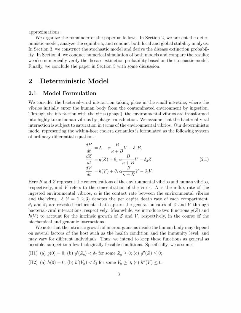
0 for all Z ≥ Zg. Thus, for each 0 < Be < B0, there always exists a unique Ze > 0 suchthat Π(Ze) = Be; for B = B0, B0 = Π(Z) always has a trivial solution Z = 0 and theunique positive solution Z = Z0 > 0 exists provided R0Z > 1 (see Figure 2). This showsthat the IFE always exists. When R0 > 1, the system (2.1) admits at most two feasiblenontrivial equilibria which depends on the values of R0Z and R0V . Specifically, the resultfor the nontrivial equilibrium solutions of the system (2.1) is summarized in the followingtheorem.

Theorem 2.1.

1. if R0Z > 1 and R0V ≤ 1, the system has a unique nontrivial virus-free equilibrium(VFE) (B0, Z0, 0);

2. if R0Z ≤ 1 and R0V > 1, the system has a unique endemic equilibrium (EE)(Be, Ze, Ve);

3. if R0Z > 1 and R0V > 1, two nontrivial equilibria coexist, the VFE and EE.

Theorem 2.1 implies that the system (2.1) has a unique EE if R0V > 1, and there is noEE if R0V ≤ 1.

6

(0,0) Z

B

B = B0

B = Be

B = Π(Z)

(a) R0Z > 1

(0,0) Z

B

B = B0

B = Be

B = Π(Z)

(b) R0Z < 1

Figure 2: The graphs of functions B = Π(Z) and B = constant.

The local stability of the IFE can be obtained by Theorem 2 of of van Den Driesscheand Watmough [25]: the IFE is locally asymptotically stable when R0 < 1 and unstablewhen R0 > 1. The following result establishes local asymptotic stability of the unique EEwhen it exists.

Theorem 2.2. If R0V > 1, the EE of the system (2.1) is locally asymptotically stable.

Proof. The Jacobian matrix of the system (2.1) at EE, (B,Z, V ) = (Be, Ze, Ve), is givenby

J =

a 0 b

θ1ακ

(κ+Be)2Ve g′(Ze)− δ2 θ1α

Be

κ+Be

c 0 d

(2.11)

where

a = −α κ

(κ+Be)2Ve − δ1

b = −α Be

κ+Be

,

c = θ2 ακ

(κ+Be)2Ve,

d = h′(Ve) + θ2 αBe

κ+Be

− δ3.

(2.12)

In view of Be > 0, Ze > 0 and Ve ≥ 0, it is clear that a < 0, b < 0 and c > 0. By direct

7

calculation, we find that the eigenvalues of J are

λ1 = g′(Ze)− δ2,

λ2 =1

2

(a+ d+

√(a− d)2 + 4bc

),

λ3 =1

2

(a+ d−

√(a− d)2 + 4bc

).

(2.13)

We now claim that (1) g′(Ze) − δ2 < 0; (2) d < 0. If this claim holds, then λ1 < 0,λ2 + λ3 = a + d < 0 and λ2λ3 = ad − bc > 0, and hence all the eigenvalues are negative.Thus, to show that the EE is locally asymptotically stable, it suffices to prove the claim issatisfied. Consider f(Z) := Π(Z)−Be, where Π(Z) is defined in (2.10). By the propertiesof Π and Ze, there exists r > 0 such that (i) f(Z) > 0 for Z ∈ (Ze−r, Ze), (ii) f(Z) < 0 forZ ∈ (Ze, Ze + r), and (iii) f ′′(Z) ≤ 0. This implies that f ′(Ze) < 0. Hence g′(Ze)− δ2 < 0.Similarly, using another function φ(V ) − ψ−1(V ) (where ψ−1 is the inverse function ofV = ψ(B)), one can verify that φ′(Ve) < (ψ−1)′(Ve), and this gives d < 0. This completesthe proof.

By the similar argument as that in the proof of Theorem 2.2, one can obtain the resultbelow regarding the local asymptotic stability of the VFE.

Theorem 2.3.

1. If R0Z > 1 and R0V ≤ 1, the VFE of the system (2.1) is locally asymptotically stable.

2. If R0Z > 1 and R0V > 1, the VFE of the system (2.1) is unstable.

In what follows, we will focus on the global stability of the equilibrium solutions ofmodel (2.1). By the first equation in (2.1),

dB

dt≤ Λ− B

δ1.

Hence lim supt→∞B(t) ≤ B0. Thus, a biologically feasible region is given by

Ω = (B,Z, V ) : 0 ≤ B ≤ B0, Z ≥ 0, V ≥ 0. (2.14)

It is easy to verify that this region is positively invariant. The following result summarizesthe global stability of the IFE.

Theorem 2.4. If R0 < 1, the IFE is globally asymptotically stable in Ω.

Proof. Since V−1 and F are nonnegative (see (2.2) and (2.3)), the Perron-Frobenius The-orem implies that the nonnegative matrix V−1F has a nonnegative left eigenvector u cor-responding to the eigenvalue R0 = ρ(FV−1) = ρ(V−1F); that is, uTV−1F = uTR0. WriteX = (Z, V )T . One can verify that

dXdt≤ (F − V)X . (2.15)

8

Motivated by [22], we construct a Lyapunov function

L = uTV−1X .

Differentiating L along the solutions of (2.1) yields

L′ = uTV−1X ′ ≤ uTV−1(F − V

)X = uT (R0 − 1)X . (2.16)

Thus, if R0 < 1, L′ = 0 implies uTX = 0. It gives Z = 0 or V = 0. When R0 < 1,equations of (2.1) and assumption (H1) yield B = B0 and V = Z = 0. Therefore, theinvariant set on which L′ = 0 contains only one point (B0, 0, 0). Applying the LaSalle’sinvariant principle [15], we see that the IFE is globally asymptotically stable in Ω if R0 < 1.

Theorem 2.5. Assume that R0 > 1.

1. If R0V > 1, then the EE is globally asymptotically stable in R3+.

2. If R0Z > 1 and R0V ≤ 1, then the VFE is globally asymptotically stable in R3+.

Proof. Note that model (2.1) can be decoupled as follows:

dB

dt= Λ− α B

κ+BV − δ1B,

dV

dt=h(V ) + θ2 α

B

κ+BV − δ3V.

(2.17)

anddZ

dt= g(Z) + θ1 α

B

κ+BV − δ2Z. (2.18)

If R0 > 1, there are two scenarios; that is, Case 1: R0V > 1; Case 2: R0V ≤ 1 and R0Z > 1.For illustration, let us consider Case 1. Model (2.1) has two equilibria when R0Z ≤ 1

or three equilibria when R0Z > 1. First, let us restrict our discussion to B-V plane andconsider the two-dimensional system (2.17). When R0Z ≤ 1, the two equilibria of (2.17)are the (B0, 0) and (Be, Ve). The former is the projection of the IFE onto B-V plane, andthe latter is that of the EE. We want to show that pe := (Be, Ve) is globally asymptoticallystable in D = (B, V ) : B ≥ 0, V ≥ 0. Clearly, no closed orbit can touch the the boundary

B = 0 or V = 0. Moreover, one can rule out closed orbits enclosing pe in D. LetD be the

interior of D, w(B, V ) = 1V∈ C1(

D), and f = (f1, f2)

T denote the vector field of (2.17).

The expression div(w · f) := (wf1)B + (wf2)V = −α κ(κ+B)2

− δ1V

+ h′(V )V−h(V )V 2 < 0 is of

one sign inD, for which h′(V )V − h(V ) ≤ 0 follows from the assumption (H2). So the

Dulac criterion [30] implies that there is no closed orbit in D. Additionally, we can rule

9

out homoclinic and heteroclinic orbits in D. Since p0 := (B0, 0) is a saddle with stablemanifold on the boundary of D and unstable manifold in D, the subsystem (2.17) cannotallow any homoclinic and heteroclinic orbits. Besides, pe is locally asymptotically stable.By the Poincare-Bendixson theorem, pe is globally asymptotically stable in D. To establishthe global stability of the EE in R3

+, it suffices to consider (2.18) with (B, V ) = (Be, Ve);namely,

dZ

dt= g(Z) + θ1 α

Be

κ+Be

Ve − δ2Z.

In view of R0Z ≤ 1 and 0 < Be < B0, based on our equilibrium analysis on the EE, weobtain limt→∞ Z(t) = Ze. This proves that the EE is globally asymptotically stable in R3

+.Using similar analysis, we can show the global stability of the EE in R3

+ when R0V > 1and R0Z > 1, and the global stability of the VFE when R0Z > 1 and R0V ≤ 1.

3 Stochastic Model

3.1 Markov Jump Process Model

If the number of human vibrios or virus is not sufficiently large, homogeneous mixing atthe beginning of the disease epidemic usually is not an appropriate assumption and therandomness should be carefully accounted. So we use a Markov jump process (MJP),which is continuous in time and discrete in the state space, to model the bacterial-viralinteraction in a more realistic way.

Let B(t), Z(t) and V (t) be discrete-valued random variables representing the numberof environmental vibrios, human vibrios and virus, respectively. It is worth to mentionthat, in realistic bacterial-viral interaction, each cell after lysis will lead to multiple humanvibrios and viruses generated and released. Thus, we will assume θ1 > 1 and θ2 > 1 inwhat follows. Following the definition of the events and transition rates summarized inTable 1, we obtain the following MJP model

B(t) = B(0) + N1

(∫ t

0

Λ du)−N2

(∫ t

0

αB(u)

κ+B(u)V (u)du

)−N3

(∫ t

0

δ1B(u) du),

Z(t) = Z(0) + N4

(∫ t

0

g(Z(u)) du)

+ N2

(∫ t

0

αB(u)

κ+B(u)V (u)du

)+ N5

(∫ t

0

(θ1 − 1)αB(u)

κ+B(u)V (u) du

)−N6

(∫ t

0

δ2Z(u) du),

V (t) = V (0) + N7

(∫ t

0

h(V (u)) du)

+ N2

(∫ t

0

αB(u)

κ+B(u)V (u) du

)+ N8

(∫ t

0

(θ2 − 1)αB(u)

κ+B(u)V (u) du

)−N9

(∫ t

0

δ3V (u) du),

(3.1)

10

where Ni9i=1 are a sequence of independent scalar Poisson process with rate 1.

Table 1: Markov jump process model with Poisson rates ri∆t+ o(∆t).

Event Description Change Rate, ri1 Recruitment of B from the environment B → B + 1 Λ

B → B − 12 Bacterial-viral interaction Z → Z + 1 α B

κ+BV

V → V + 13 Death of B B → B − 1 δ1B4 Replication of Z Z → Z + 1 g(Z)5 Production of Z due to bacterial-viral interaction Z → Z + 1 (θ1 − 1)α B

κ+BV

6 Death of Z Z → Z − 1 δ2Z7 Viral growth V → V + 1 h(V )8 Production of V due to bacterial-viral interaction V → V + 1 (θ2 − 1)α B

κ+BV

9 Death of V V → V − 1 δ3V

3.2 Disease Extinction Probability

We will now approximate the dynamics of the nonlinear MJP (3.1) and estimate theextinction probability of the disease near the IFE by using a Galton-Watson multitypebranching process (BGWbp) [1, 8, 10,14]. Since the disease groups are human vibrios andvirus, the branching process approximation is applied to these two groups at the IFE andthe environmental vibrios are assumed to sufficiently close to B0 = Λ/δ1.

In general, given xi(0) = 1 and xj(0) = 0 (j 6= i), the offspring probability generatingfunction (pgf) fi : [0, 1]n → [0, 1]n is defined as

fi(x1, x2, . . . , xn) =∞∑k1=1

. . .∞∑

kn=1

Pi(k1, . . . , kn)xk11 . . . xknn , (3.2)

where Pi(k1, . . . , kn) is the probability that one type i individual gives “birth” to kj indi-viduals of type j. For our model, the offspring pgf for Z, given Z(0) = 1 and V (0) = 0,is

f1(x1, x2) =gZx

21 + δ2

gZ + δ2; (3.3)

the offspring pgf for V , given Z(0) = 0 and V (0) = 1, is

f2(x1, x2) =

(hV + θ2α

B0

κ+B0

)x22 + θ1α

B0

κ+B0x1x2 + δ3

hV + (θ1 + θ2)αB0

κ+B0+ δ3

, (3.4)

11

for which we have linearly approximated g(Z).= gZZ and h(V )

.= hV V , as Z and V are

close to zero and g(0) = h(0) = 0. Hence, the expectation matrix M = (mij) can bewritten as

M =

2 gZ

gZ + δ20

θ1αB0

κ+B0

hV + (θ1 + θ2)αB0

κ+B0+ δ3

2(hV + θ2α

B0

κ+B0

)+ θ1α

B0

κ+B0

hV + (θ1 + θ2)αB0

κ+B0+ δ3

, (3.5)

for which mij =∂fi∂xj

∣∣∣(x1,x2)=(1,1)

(1 ≤ i, j ≤ 2). The branching process is supercritical (resp.

critical, subcritical) when ρ(M) > 1 (resp. = 1, < 1). It follows from direct calculationthat

ρ(M) = maxm11,m22

= max

2R0Z

R0Z + 1,

2R0V + c

R0V + 1 + c

, (3.6)

where c =(θ1α

B0

κ+B0

)/δ3. Since M is reducible, one can not apply the Threshold Theorem

in [2] to obtain the relationship between the stochastic threshold ρ(M) and the determin-istic threshold R0. Fortunately, by direct calculation, one can verify that the ThresholdTheorem also holds for our case, i.e.,

ρ(M) < 1 (= 1, > 1) ⇐⇒ R0 < 1 (= 1, > 1). (3.7)

The following theorem summarizes the result on the ultimate extinction probability ofthe BGWbp.

Theorem 3.1. Let P0(z0, v0) = limt→∞ P(Z(t) = V (t) = 0|Z(0) = z0, V (0) = v0) denoteultimate extinction probability within a human host. Let P ext

0 = P ext0 (z0, v0) denote the

branching process estimate of the extinction probability P0(z0, v0).

1. If R0 < 1, then P ext0 = 1.

2. Assume R0 > 1.

(a) If R0Z ≤ 1 and R0V > 1, then P ext0 =

( 1

R0V

)v0;

(b) If R0Z > 1 and R0V ≤ 1, then P ext0 =

( 1

R0Z

)z0;

(c) If R0Z > 1 and R0V > 1, then P ext0 =

1

(R0Z)z0(q2∗)v0.

where

q2∗ =

1

2

1 +1

R0V

+1

RE

−

√(1− 1

R0V

+1

RE

)2

+ 41

R0VRE

with RE =

[hV/(

α B0

κ+B0

)+ θ2

]/[θ1(1− 1/R0V )].

12

Proof. The minimal fixed point (q1, q2) of

fi(x1, x2) = xi, (i = 1, 2) (3.8)

on [0, 1]2 determines the extinction probability of the infection; that is P ext0 = qz01 q

v02 . By

the theory of branching process [1, 4, 8, 10, 13] and the relationship in (3.7), part 1 followsimmediately and it remains to prove part 2. Suppose R0 > 1. Note that (1, 1) is always afixed point and no fixed point satisfies q1q2 = 0. It suffices to show that (3.8) has a uniquefixed point in (0, 1]2 − (1, 1). Since the matrix M is reducible, there is not necessarilya unique fixed point in (0, 1)2 in the supercritical case [4, 10]. Solving (3.8), we find thatindeed there are four fixed points (1, 1), (q∗1, 1), (1, q∗2) and (q∗1, q2

∗), where q∗1, q∗2 and q2

∗ aredefined as

q∗1 =δ2gZ

=1

R0Z

,

q∗2 =δ3

hV + θ2αB0

κ+B0

=1

R0V

,

q2∗ =

1

2

1 +1

R0V

+1

RE

−

√(1− 1

R0V

+1

RE

)2

+ 41

R0VRE

,

(3.9)

with RE =hV /

(α B0

κ+B0

)+ θ2

θ1(1− 1/R0V ).

Thus, when R0 > 1, we can conclude the existence of a unique fixed point (q1, q2) in(0, 1]2 − (1, 1) by considering the following three cases: (a) if R0Z ≤ 1 and R0V > 1,(q1, q2) = (1, q∗2); (b) if R0Z > 1 and R0V ≤ 1, (q1, q2) = (q∗1, 1); (c) if minR0Z , R0V > 1,(q1, q2) = (q∗1, q2

∗) ∈ (0, 1)2. By (3.9), the result follows .

Remark: Any event other than disease extinction can be loosely regarded as an infec-tion outbreak [1, 2, 12]. Let Pout denote the branching process estimate of the probabilityof a disease outbreak. Thus, Theorem 3.1 implies that

(a). If R0Z ≤ 1 and R0V > 1, then Pout = 1−( 1

R0V

)v0;

(b). If R0Z > 1 and R0V ≤ 1, then Pout = 1−( 1

R0Z

)z0;

(c). If R0Z > 1 and R0V > 1, then Pout = 1− 1

(R0Z)z0(q2∗)v0 .

This shows that the probability of a cholera infection outbreak depends not only on theinitial numbers of bacteria and/or viruses, but also on the risk factors due to the intrinsicgrowth of human virbrios and/or the bacterial-viral interaction.

13

0 20 40 600

1

2

3

4

5

6x 10

5

Time (hours)

R0Z

= 0.6; R0V

= 0.5

B

Z

V

(a)

0 20 40 600

2

4

6

8

10

12

x 105

Time (hours)

R0Z

= 2.1; R0V

= 0.5

B

Z

V

(b)

0 20 40 600

5

10

15

20x 10

5

Time (hours)

R0Z

= 0.6; R0V

= 2.4

B

Z

V

(c)

0 20 40 600

1

2

3

4x 10

6

Time (hours)

R0Z

= 1.3; R0V

= 1.3

B

Z

V

(d)

Figure 3: A sample path of the stochastic model (3.1) (displayed in solid curves) vs.the associated solution of the ODE model (2.1) (displayed in dashed curves). In thisexample, we take the logistic growth to depict the intrinsic growth of Z and V . Morespecifically, g(Z) = g0Z(1 − Z/κZ) and h(V ) = h0V (1 − V/κV ). The values of parame-ters are: λ = 105 cells· ml−1hour−1, κ = 106 cells· ml−1, κZ = 2 × 106 cells· ml−1, κV =108 cells· ml−1, δ1 = δ2 = 7/30 hour−1, δ3 = 7/3 hour−1, α = 1 hour−1, θ1 = 1; (a)θ2 = 2, g0 = 0.15, h0 = 0.6; (b) θ2 = 2, g0 = 0.5 hour−1, h0 = 0.6 hour−1 ; (c)θ2 = 15, g0 = 0.15 hour−1, h0 = 1 hour−1; (d) θ2 = 2, g0 = 0.3 hour−1, h0 = 2 hour−1.

4 Numerical Simulations

In this section, we numerically solve the ODE model (2.1) and stochastic model (3.1),where the parameter values for the environmental vibrios are obtained from the literature

14

0 20 40 600

5

10

15x 10

5

Time (hours)

R0Z

= 2.1; R0V

= 0.5

B

Z

V

(a)

0 1 2 3 4 50

2

4

6

8

10

Time (hours)

R0Z

= 2.1; R0V

= 0.5

B

Z

V

(b) Enlarge Figure 4 (a) near the origin

0 20 40 600

5

10

15

20x 10

5

Time (hours)

R0Z

= 0.6; R0V

= 2.4

B

Z

V

(c)

0 10 20 30

5

10

15

20

Time (hours)

R0Z

= 0.6; R0V

= 2.4

B

Z

V

(d) Zoom in Figure 4 (c) near the origin

0 20 40 600

1

2

3

4x 10

6

Time (hours)

R0Z

= 1.3; R0V

= 1.3

B

Z

V

(e)

0 2 4 6 8 10 12

5

10

15

20

Time (hours)

R0Z

= 1.3; R0V

= 1.3

B

Z

V

(f) Enlarge Figure 4 (e) near the origin

Figure 4: Illustration of disease extinction by displaying a sample path of the stochasticmodel (3.1) as compared to the corresponding ODE solution of (2.1). Here the solid anddashed curves represent a sample path of the stochastic model and the associated ODEmodel, respectively. It shows that the ODE solution approaches the VFE (see the toppanel) or EE (see the middle and bottom panels), whereas the corresponding sample pathof the stochastic model can go to extinction (see the panel on the right). The parametervalues are the same as that of Figure 3. Initial conditions: (a) (B,Z, V )(0) = (2×104, 8, 2);(b) and (c) (B,Z, V )(0) = (2× 104, 5, 5).

15

(e.g., see [27] and the reference therein). On the other hand, we have not been able tofind useful quantitative measurements regarding the bacterial-viral dynamics within thehuman body and, thus, the parameter values associated with the bacterial-viral interactionare assumed in our simulation. Our numerical results, presented below, could serve as atheoretical means to justify that our assumptions are biologically feasible. Figures 3-4illustrate the dynamics of our ODE model (2.1) and stochastic model (3.1). In bothfigures, the dashed and solid curves represent the solution of the deterministic model andan associated stochastic sample path, respectively. Particularly, Figure 3 demonstratesthat Monte Carlo simulation of stochastic model (3.1) can be close to the correspondingODE solution in all of the four scenarios; Figure 4 illustrates the occurrence of diseaseextinction whereas the ODE model indicates global stability of the VFE/EE.

Case 1: R0Z < 1 and R0V < 1. This is illustrated in Figure 3 (a), and R0Z = 0.6 andR0V = 0.5 in the displayed example. It shows that sample paths of our stochastic modelare very likely to be close to the associated deterministic solution, and both deterministicand stochastic models indicate the disease extinction. Moreover, in this case, for everyset of parameter values within biologically feasible ranges, and for initial conditions thatare near the IFE, we have numerically confirmed that the disease extinction probability isvery close to one. Here, extinction probability is estimated by computing the proportionof 10, 000 sample paths that hit zero. When initial conditions are not close to the IFE, forinstance, (B,Z, V )(0) = (6×103, 105, 105), sample paths of stochastic model are still likelyto fluctuate around the associated ODE solution. Meanwhile, we see from this examplethat the virus population decays exponentially and approaches to zero in about 5 hours,and human vibrios population decreases linearly and goes to zero after 66 hours or so.This sample path indicates that disease extinction within a human host occurs in about66 hours.

Case 2: R0Z > 1 and R0V < 1. As one can see from Figure 3 (b), the ODE solu-tion converges to the VFE and hence the deterministic model indicates the persistenceof environmental and human bacteria. In contrast, the stochastic model shows bacteriumpopulations can either persist (displayed in Figure 3 (b)), or go extinct (displayed in Figure4 (a)-(b)). Case 3: R0Z < 1 and R0V > 1 and Case 4: R0Z > 1 and R0V > 1. In both sce-narios, deterministic dynamics indicate the occurrence of an outbreak, which is illustratedin Figures 3 (c)-(d), and 4 (c)(e). However, the stochastic model, more realistically, showsthat disease can go extinct within the human host (illustrated in Figure 4 (c)-(f)). Indeed,Theorem 3.1 demonstrates that this extinction has a positive probability.

Let P ext0 denote the probability of disease extinction computed from the branching

process approximation. Let PMC0 be an estimate obtained from the fraction of sample

paths (out of 10, 000) in which both Z(t) and V (t) hit zero before reaching VFE/EElevels. Applying Theorem 3.1, we calculate explicit estimate P ext

0 and then compare tothe corresponding estimate PMC

0 obtained from Monte Carlo simulation. A summaryof results for various initial conditions in Cases 2-4 are displayed in Table 2. It showsthat P ext

0 is a good estimate of the disease extinction probability. For instance, in the

16

Table 2: Disease extinction probability estimated by using the branching process approx-imation, P ext

0 , vs. the associated estimate based on Monte Carlo simulations of 10, 000sample paths of (3.1), PMC

0 . The parameter values are the same as that of Figure 3.

Scenario z0 v0 P ext0 PMC

0

R0Z = 0.64, R0V = 2.36 1 1 0.4242 0.42361 2 0.1800 0.17822 1 0.4242 0.4291

R0Z = 2.14, R0V = 0.51 1 1 0.4667 0.46531 2 0.4667 0.46012 1 0.2178 0.2209

R0Z = 1.29, R0V = 1.29 1 1 0.6508 0.65231 2 0.5446 0.54292 1 0.5062 0.5107

first example, R0Z = 0.64 < 1, R0V = 2.36 > 1, and V (0) = v0 = 1. By Theorem3.1, P ext

0 = (1/R0V )v0 = 0.4242. Comparing this with PMC0 = 0.4236, we see that the

theoretical approximation P ext0 is very close to its numerical approximation PMC

0 based onsample paths.

5 Discussion

We have proposed a new modeling framework for the within-host dynamics of cholera, usingboth deterministic and stochastic formulations. Our focus is the interaction of environ-mental vibrios (with low infectivity), human vibrios (with high infectivity), and the virus(which causes the transformation from environmental vibrios to human vibrios) withina human host. Such an interaction is critical in shaping the evolution of the pathogenwithin human body and directly contributes to the epidemiology of cholera at the popula-tion level, since the human vibrios shed out of human body will remain highly infectiousfor a certain period of time and can be transmitted among human hosts.

For our deterministic model, we have calculated the basic reproduction number, R0,which consists of two components: one represents the intrinsic growth of the human vibriosand the other accounts for the viral-bacterial interaction. We have established the basicreproduction number as a sharp threshold for disease dynamics: when R0 < 1, the highlyinfectious vibrios will not grow within the human host and the environmental vibriosingested into human body will not cause cholera infection; when R0 > 1, the humanvibrios will grow and persist, leading to human cholera. We have found that while thereis only one equilibrium (the IFE) when R0 < 1, there can be two or three equilibria whenR0 > 1 that include the IFE and one or both of the VFE and EE. The existence and

17

stabilities of these equilibria characterize the essential dynamics of the model, and we haveconducted both local and global stability analysis for each equilibrium.

For our stochastic model, based on the Markov jump process, we have focused ourattention on the probability of disease extinction within a human host which provides anestimate of the disease risk under some realistic conditions (e.g., small amount of initialinfection, small number of bacteria or virus). We have derived an explicit expression forthe probability of disease extinction, and verified the result through careful numericalsimulation involving a large number of sample paths. We have also carefully compared thenumerical simulation results from the deterministic model and the stochastic model.

As can be expected, analysis of our deterministic model can provide more detailedinformation regarding the disease dynamics, and a single quantity, R0, can be used as adisease threshold. Nevertheless, the stochastic model can provide an important estimate ofthe disease risk under situations where the assumption of homogeneous mixing of bacteriaor virus does not hold and where the randomness should be taken into account. Hence, bothmodels are useful in studying cholera and, together, they could give us a more completepicture toward understanding the within-host dynamics of cholera.

Our future plan is to couple this within-host modeling framework with an epidemio-logical cholera model, linking the within-host and between-host dynamics of cholera in amore biologically meaningful way. Using such an integrated model, we will carefully inves-tigate the bacterial-viral interaction within human host, the human-human and human-environment interaction at the population level, and their impacts to each other towardshaping the complex, multi-scale dynamics of cholera. We will again explore both deter-ministic and stochastic formulations, and compare and integrate the findings from eachapproach.

Acknowledgments

The authors would like to thank the anonymous reviewers and the editor for their sugges-tions that have improved this paper. This work was partially supported by a grant fromthe Simons Foundation (#317047 to Xueying Wang). Jin Wang was partially supportedby the National Science Foundation under Grant Nos. 1412826, 1520672 and 1557739.

References

[1] L.J.S. Allen, and G. E. Lahodny Jr., Extinction thresholds in deterministic andstochastic epidemic models, J. Biol. Dyn. 6 (2012), pp. 590-611.

[2] L.J.S. Allen and P. van den Driessche, Relations between deterministic and stochasticthresholds for disease extinction in continuous- and discrete-time infectious diseasemodels, Math. Biosci. 243 (2013), pp. 99-108.

18

[3] R. M. Anderson and R.M. May, Infectious Diseases of Humans: Dynamics and Con-trol, Oxford University Press, 1991.

[4] K.B. Athreya and P.E. Ney, Branching Processes, Springer-Verlag, New York, 1972.

[5] V. Capasso, S. L. Paveri-Fontana, A mathematical model for the 1973 cholera epidemicin the European Mediterranean region, Rev. Epidemiol. Sante, 27(2) (1979), pp. 121-132, 1979.

[6] A. Carpenter, Behavior in the time of cholera: Evidence from the 2008-2009 choleraoutbreak in Zimbabwe, In Social computing, behavioral-cultural modeling and predic-tion, vol. 8393 (eds Kennedy WG, Agarwal N, Yang SJ), pp. 237-244. Lecture Notesin Computer Science. Berlin, Germany: Springer International Publishing.

[7] R. R. Colwell, A global and historical perspective of the genus Vibrio, in The Biologyof Vibrios, F.L. Thompson, B. Austin, and J. Swings (eds.), ASM Press, WashingtonDC, 2006.

[8] K. S. Dorman, J.S. Sinsheimer, and K. Lange, In the garden of branching processes,SIAM Rev. 46 (2004), pp. 202229.

[9] S. M. Faruque1 and G.B. Nair, Vibrio cholerae: Genomics and Molecular Biology,Caister Academic Press, 2008.

[10] T. E. Harris, The Theory of Branching Processes, Springer-Verlag, Berlin, 1963.

[11] D. M. Hartley, J. G. Morris, D. L. Smith, Hyperinfectivity: a critical element in theability of V. cholerae to cause epidemics? PLoS Med., 3 (2006), pp. 0063-0069.

[12] O.A. van Herwaarden and J. Grasman, Stochastic epidemics: major outbreaks and theduration of the endemic period, J. Math. Biol. 33 (1995), pp. 581-601.

[13] P. Jagers, Branching Processes with Biological Applications, John Wiley & Sons, Lon-don and New York, 1975.

[14] S.T. Karlin, H.M. Taylor, A First Course in Stochastic Processes, second ed., Aca-demic Press, San Diego, CA, 1975.

[15] J. P. LaSalle, The Stability of Dynamical Systems, Regional Conference Series inApplied Mathematics, SIAM, Philadelphia, 1976.

[16] Z. Mukandavire, S. Liao, J. Wang, H. Gaff, D. L. Smith, J. G. Morris, Estimating thereproductive numbers for the 2008-2009 cholera outbreaks in Zimbabwe, P. Nat. Acad.Sci. USA, 108 (2011), pp. 8767-8772.

19

[17] R. L. M. Neilan, E. Schaefer, H. Gaff, K. R. Fister, S. Lenhart, Modeling optimalintervention strategies for cholera, B. Math. Biol., 72 (2010), pp. 2004-2018.

[18] E. J. Nelson, J. B. Harris, J. G. Morris, S.B. Calderwood, and A. Camilli, Choleratransmission: the host, pathogen and bacteriophage dynamics, Nature Reviews: Mi-crobiology, 7 (2009), pp. 693-702.

[19] D. Posny and J. Wang, Modelling cholera in periodic environments, J. Biol. Dyn., 8(1)(2014), pp. 1-19.

[20] D. Posny, J. Wang, Z. Mukandavire and C. Modnak, Analyzing transmission dynamicsof cholera with public health interventions, Math. Biosci., 264 (2105), pp. 38-53.

[21] Z. Shuai, P. van den Driessche, Global dynamics of cholera models with differentialinfectivity, Math. Biosci., 234(2) (2011), pp. 118-126.

[22] Z. Shuai, P. van den Driessche, Global stability of infectious disease models usingLyapunov functions, SIAM J. Appl. Math., 73(4) (2013), pp. 1513-1532.

[23] J. P. Tian, J. Wang, Global stability for cholera epidemic models, Math. Biosci., 232(1)(2011), pp. 31-41.

[24] J. H. Tien, D. J. D. Earn, Multiple transmission pathways and disease dynamics in awaterborne pathogen model, B. Math. Biol., 72(6) (2010), pp. 1506-1533.

[25] P. van den Driessche and J. Watmough, Reproduction numbers and sub-thresholdendemic equilibria for compartmental models of disease transmission. MathematicalBiosciences 180 (2002), pp. 29-48.

[26] J. Wang, S. Liao, A generalized cholera model and epidemic-endemic analysis, J. Biol.Dyn., 6(2) (2012), pp. 568-589.

[27] X. Wang, J. Wang, Analysis of cholera epidemics with bacterial growth and spatialmovement, J. Biol. Dyn., 9(1) (2015), pp. 233-261.

[28] X. Wang, J. Wang, Disease dynamics in a coupled cholera model linking within-host and between-host interactions, to appear in journal of Biological Dynamics,DOI:10.1080/17513758.2016.1231850.

[29] X. Wang, D. Gao, J. Wang, Influence of human behavior on cholera dynamics, Math.Biosci., 267 (2015), pp. 41-52.

[30] S. Wiggins, Introduction to Applied Nonlinear Dynamical Systems and Chaos,Springer, 2nd edition, 2003.

20

[31] K. Yamazaki, X. Wang, Global well-posedness and asymptotic behavior of solutions toa reaction-convection-diffusion cholera epidemic model, Discrete Contin. Dyn. Syst.Ser. B, 21 (2016), pp. 1297-1316.

[32] K. Yamazaki and X. Wang. Global stability and uniform persistence of the reaction-convection-diffusion cholera epidemic model, Mathematical Biosciences and Engineer-ing, 14:2 (2017), pp. 559-579.

21