MODELING THE WESTERN LAKEERIE WALLEYE POPULATION:

A FEASIBILITY STUDY

B. J. SHUTERInstitute for Environmental Studies and

Department of ZoologyUniversity of Toronto

Toronto, Ontario M5S 1A4

J. F. KOONCEDepartment of Biology

Case Western Reserve UniversityCleveland, Ohio 44106

and

H. A. REGIERInstitute for Environmental Studies and

Department of ZoologyUniversity of Toronto

Toronto, Ontario M5S 1A4

TECHNICAL REPORT NO. 32

Great Lakes Fishery Commission

1451 Green RoadAnn Arbor, Michigan 48107

April 1979

FOREWORD

The Great Lakes Fishery Commission is participating in a series ofsymposia whose subject matter bears on Great Lakes fisheries: SalmonidCommunities in Oligotrophic Lakes (SCOL), July 1971; the Percid Inter-national Symposium (PERCIS), 24 September-5 October 1976; A Symposiumon Selected Coolwater Fishes of North America, 7-9 March 1978; the SeaLamprey International Symposium (SLIS), scheduled for l-10 August 1979;and the Stock Concept Symposium, scheduled for 1980.

After concise versions of SCOL papers had been published in theJournal of the Fisheries Research Board of Canada (volume 29, number 6,June 1972), it was clear that much detailed information that had beendeveloped by the authors and refined by events at the symposium, and whichwould be of very considerable value to fishery workers in the Great Lakesarea, would not be generally available. The Commission therefore invited theauthors of case histories on seven lakes-Superior, Michigan, Huron, Erie,Ontario, Opeongo, and Kootenay-to publish full versions in the Commission’sTechnical Report series (numbers 19-25, 1973).

Similarly, after concise versions of PERCIS papers were published in theJournal of the Fisheries Research Board of Canada (volume 34, number 10,October 1977) the Commission asked symposium participants and authors ofpapers dealing specifically with Great Lakes percids whether more detailed ver-sions of certain papers should be published for the benefit of present and futurefishery workers. Based in part on the replies, the Commission authorizedpublication of Technical Reports 31 and 32: “Walleye stocks in the GreatLakes, 1800-1975: fluctuations and possible causes,” by J. C. Schneider and J.H. Leach; and “Modeling the western Lake Erie walleye population: afeasibility study,” by B. J. Shuter, J. F. Koonce, and H. A. Regier.

Carlos M. Fetterolf, Jr.Executive Secretary

CONTENTS

Abstract . . . . . . . . . . . . . . . . . . . . . . . . . . . . . . . . . . . . . . . . . . . . . . . . . . . . . . 1

Introduction . . . . . . . . . . . . . . . . . . . . . . . . . . . . . . . . . . . . . . . . . . . . . . . . . . . 1

Data base: sources and preliminary manipulations . . . . . . . . . . . . . . . . . . 3Abundanceindices.. . . . . . . . . . . . . . . . . . . . . . . . . . . . . . . . . . . . . . . . 3Annual survival rates . . . . . . . . . . . . . . . . . . . . . . . . . . . . . . . . . . . . . . . 7Spring water temperature data . . . . . . . . . . . . . . . . . . . . . . . . . . . . . . . 8

Stock-recruitment relation . . . . . . . . . . . . . . . . . . . . . . . . . . . . . . . . . . . . . . 9

Relations between growth rate and population density . . . . . . . . . . . . . . . 15

Structure and behavior of the population model . . . . . . . . . . . . . . . . . . . . 16

Evaluation of analyses and simulation studies . . . . . . . . . . . . . . . . . . . . . . 20

Analysis of alternative harvest strategies . . . . . . . . . . . . . . . . . . . . . . . . . . 23Cohort yield model . . . . . . . . . . . . . . . . . . . . . . . . . . . . . . . . . . . . . . . . . 23Stochastic population yield model . . . . . . . . . . . . . . . . . . . . . . . . . . . . 25Stochastic dynamic programming analysis . . . . . . . . . . . . . . . . . . . . . 28

Evaluation of optimal harvest strategies . . . . . . . . . . . . . . . . . . . . . . . . . . . 31

Conclusions.. . . . . . . . . . . . . . . . . . . . . . . . . . . . . . . . . . . . . . . . . . . . . . . . ..3 1

Acknowledgments . . . . . . . . . . . . . . . . . . . . . . . . . . . . . . . . . . . . . . . . . . . ..3 1

References.. . . . . . . . . . . . . . . . . . . . . . . . . . . . . . . . . . . . . . . . . . . . . . . . . ..3 2

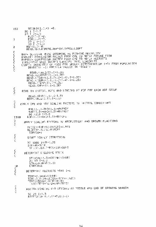
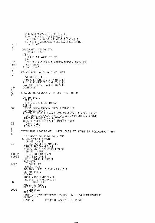
Appendix A. Western Lake Erie walleye population model . . . . . . . . . 35

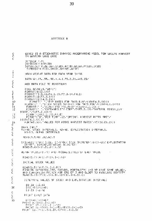
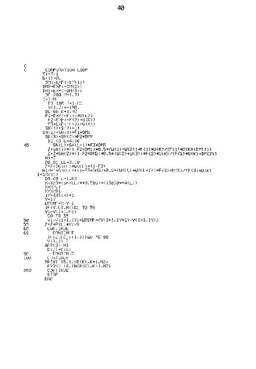
Appendix B. Stochastic dynamic programming model for walleyeharvest in western Lake Erie . . . . . . . . . . . . . . . . . . . . . . . . . . . . . . . . . . 39

MODELING THE WESTERN LAKE ERIEWALLEYE POPULATION: A FEASIBILITY STUDY

B. J. Shuter!‘J. F. Koonce, and H. A. Regier

ABSTRACT

A simple population model of the walleye (Stizostedion vitreum vitreum) of westernLake Erie was constructed from a set of empirical relationships linking growth to populationdensity and recruitment to breeding stock size and the spring water temperature regime.Given a reasonable set of values for annual rates of natural and fishing mortalities, consis-tent with empirical estimates of total survival for the period 1947-75, the model generated apattern of behavior similar, both qualitatively and quantitatively, to that exhibited by thereal population. Two types of stochastic models, based on the initial population model, wereused to derive optimal harvest strategies for the population. These strategies were notsensitive to variations in catchability and natural mortality, but the estimated yields pro-duced were highly sensitive to variations in both these factors. A refined and extendedversion of this model may be useful in developing management policies for this population.

INTRODUCTION

For well over a century, the western Lake Erie population of thewalleye (Stizostedion vitreum vitreum) has been subjected to a variety ofanthropogenic stresses. These have included a substantial reduction inavailable spawning areas (Langlois 1945; Regier et al. 1969) and a signifi-cant increase in the rate of exploitation (Regier et al. 1969).

Historically, walleyes spawned in many of the western Lake Erietributaries, in shallow nearshore areas, and on offshore reefs (Langlois1945; Regier et al. 1969). By the early 1940’s, most of the stream spawningareas had been destroyed by dam construction, siltation, pollution, orirregularity of streamflow caused by man’s activities (Langlois 1945). Bythe late 1940’s many of the inshore areas had suffered a similar fate(Regier et al. 1969), and only the offshore reefs remained as significantspawning areas (Hartman 1973; Leach and Nepszy 1976). Unfortunately,these mid-lake spawning reefs are vulnerable to a variety of adverse fac-tors such as water currents, turbulence, and temperature reversals. Theapparent dependence of the strength of recent year classes on the rate of

1 Present address: Ministry of Natural Resources, Fisheries Branch, Box 50, Maple, OntarioLOJ 1EO.

water temperature increase during the spring spawning season can beexplained in part by this susceptibility of eggs laid on reefs to destructionby relatively common environmental disturbances (Busch et al. 1975).

Concurrent with, and following, the destruction of the inshorespawning areas, the annual walleye harvest in western Lake Erie variedconsiderably: the commercial catch remained nearly constant at about 1million kg per year until the mid-1930’s; began to increase slowly, reach-ing 2.6 million kg in 1950; rose rapidly to an extreme peak of 7 million kgin 1956; and then fell precipitously to less than 0.5 million kg in 1961. Itremained low until 1969, when the commercial fishery was closed becauseof mercury contamination. The rapid increase in production, beginning inthe early 1950’s, was accompanied by a significant increase in the rate ofexploitation. It has been suggested (Regier et al. 1969) that standardizedfishing effort for walleyes in Canadian waters was perhaps 50 timesgreater in the late 1950’s than in the late 1940’s.

These variations in the commercial catch were accompanied by sev-eral significant changes in the walleye population and the fishery: a pro-gressive decline in catch per unit effort (Table 1); a sharp decline in year-class strength (Parsons 1970; Regier et al. 1969); a truncation of the age

Table 1, Summary of data on annual trap-net catch of walleyes per unit effort (kg/lift) for allstatistical districts in western Lake Erie. Data in italics are from Regier

et al. (1%9) and the others are from Kutkuhn et al. (1976).

Year Mich. 0-1

Statistical districta

0-2 0E-1 0E-2

19481949195019511952195319541955195619571958195919601%11%21%319641%51966I%7I%81%9

-

-27.133.848.532.047.351.856.542.718.814.510.78.0

16.520.912.912.942.219.213.1

15.919.820.320.016.023.520.730.530.823.618.7

7.28.3 8.41.9 5.3

3.78.05.64.43.55.6

17.69.0

--------

-2.63.32.94.53.22.32.54.04.42.5

--

8.812.617.314.719.029.018.6 22.912.1 12.38.5 8.42.9 2.92.7 2.72.7 2.7

1.52.21.23.12.96.31.82.3

5.45.06.26.55.75.16.05.76.64.21.70.950.590.500.680.770.590.861.01.0--

a See Smith et al. (l%l) for detailed boundaries of districts. Districts O-l and O-2 include Ohiowaters west of Fairport, and districts 0E-1 and 0E-2 include Ontario waters west of theboundary of Elgin and Kent counties.

2

distribution (Busch et al. 1975; Parsons 1970); and a progressive increasein length at age (Parsons 1970). In the years after the ban on commercialfishing, most of these trends have reversed.

As noted by Regier et al. (1969), this set of events conforms closely tothe typical pattern expected during the “fishing-up” period (Ricker 1975)which generally follows a significant increase in exploitation rate. Therecent authors who have reviewed the history of this population (Busch etal. 1975; Hartman 1973; Nepszy 1977; Regier et al. 1969) seem to be ingeneral agreement that the rate of exploitation reached nonsustainablelevels in the mid-1950’s and that this was a primary, if not the major,factor responsible for some or all of the changes listed above.

Combining this interpretation of events with the known dependenceof year-class strength on the spring warming rate leads to a rather simplequalitative model of the population consisting of two major elements: astandard, hump-shaped stock-recruitment relation, modified by the influ-ence of the spring warming rate; and a negative relation between growthrate and population size, offset by a positive relation between growth rateand forage density. In this paper, we attempt to carry out three objec-tives: (1) evaluate the data base for the population to determine if suffi-cient information exists for the derivation of quantitative estimates ofthese basic relations; (2) incorporate the estimated relations into a quanti-tative dynamic model of the population and determine if its behavior isconsistent with observed behavior; and (3) explore some of the ways inwhich such a quantitative model could be used in managing the popula-tion. The supporting data and the methodology are given in much greaterdetail than in the earlier summary by Shuter and Koonce (1977).

DATA BASE: SOURCES AND PRELIMINARY MANIPULATIONS

The character and origins of the data base are summarized in Table 2.The relations of interest have stock abundance, or the abundance of somepart of the stock, as the independent variable or the dependent variable,or both. Therefore, it was essential to develop closely comparable indicesof stock abundance for as many years as possible.

Abundance indices

Following other authors (Kutkuhn et al. 1976; Parsons 1970; Regieret al. 1969), we assumed that data from commercial trap-net catches inUnited States waters provided the most reliable available information onlong-term changes in the population. Concurrent information on the catchper unit effort (CPE) in kilograms per lift, age distribution, and meanweight per fish was available for both fall and spring catches in Michiganand statistical district O-l (Smith et al. 1961) of western Ohio (Tables 3 and4). Unfortunately, the spring series was short (1962-69) and the fall series

3

Table 2. Types and sources of primary data sets relating to the western Lake Erie walleye.

Information Period Source

Catch and effort databy gear, statistical district,year, and season

Age compositions of commercialcatches by gear, statisticaldistrict, year, and season

Mean weights of fish infall trap-net catches

Catch indices for young-of-the-year

Lengths at various ages

Weights at various ages

Lengths and ages at maturity

Spring water temperatures

193949a

1943-7oa

1943-62

1959-7s

i92047a

1%2-66

192749

19s74a

Regier et al. (1%7, 1%9),Kutkuhn et al. (1976)

Busch et al. (1975), Parsons(1970), Kutkuhn et al. (1976)

Parsons (1970)

Kutkuhn et al. (1976)

Adamstone (1922) Deason(1933), Lawler (1948) Parsons(1970, 1972), Wolfert (1977)

Regier et al. (1%9),Kutkuhn et al. (1976)

Deason (1933), Wolfert (1%9)

Anonymous (l%l), OhioDepartment of NaturalResources (unpublished data)

a Data lacking for some years in period.

was incomplete in both districts. The following manipulations were car-ried out to extend and complete the fall CPE series for 1948-69 in Ohioand 1946-69 in Michigan.

In Ohio for 1960-69, the total fall catch was taken almost entirely withtrap nets (Kutkuhn et al. 1976) and the fall trap-net effort was highlycorrelated (r = 0.87, 12 = 10) with the total trap-net effort for the year.Assuming these relations to hold for 1948-59, we derived estimates (Table3) of the fall CPE for this period from the annual trap-net effort and falltrap-net catch data given by Kutkuhn et al. (1976) and Regier et al. (1967,1969).

Estimates (Table 3) of the fall CPE in Michigan for 1946-50 werederived as follows: the total fall catch was multiplied by the fraction of theannual catch taken in trap nets to estimate the fall trap-net catch (datafrom Regier et al. 1967); and the fall effort was assumed to have remainedconstant at 662 lifts, the mean fall effort for 1951-59.

To derive concurrent indices of relative abundance for different agegroups (i.e., number of walleyes caught per trap-net lift) from the CPEdata, we also needed to know the mean weight and the age distribution offish in the catch for each year. Such detailed information was available forall of the spring catches in Michigan and western Ohio (Table 4) and forthe fall catches for 1943-69 in Ohio and 1963-69 in Michigan (Table 3).Regression analysis showed the Michigan observations to be closely simi-lar, both qualitatively and quantitatively, to those made in Ohio over the

4

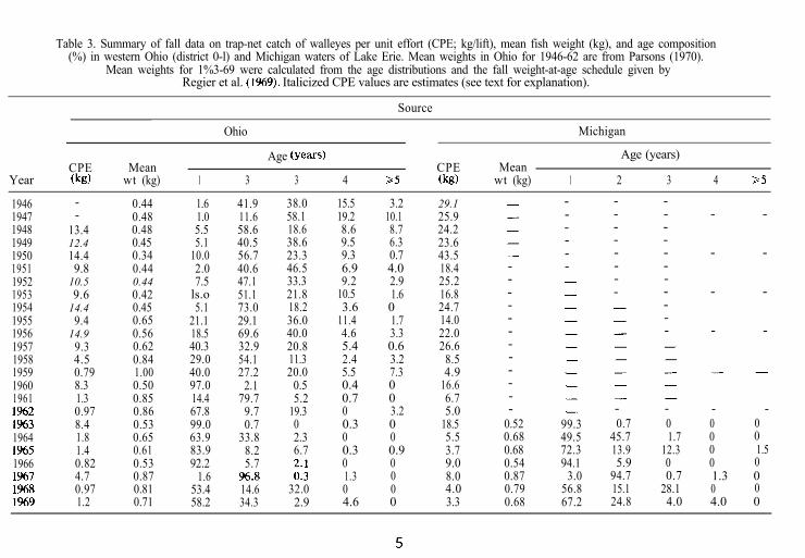
Table 3. Summary of fall data on trap-net catch of walleyes per unit effort (CPE; kg/lift), mean fish weight (kg), and age composition(%) in western Ohio (district 0-l) and Michigan waters of Lake Erie. Mean weights in Ohio for 1946-62 are from Parsons (1970).

Mean weights for 1%3-69 were calculated from the age distributions and the fall weight-at-age schedule given byRegier et al. (1%9). Italicized CPE values are estimates (see text for explanation).

Source

YearCPE Mean(kid wt (kg) 1

Ohio Michigan

Age (w-9 Age (years)CPE Mean

3 3 4 >5 (W wt (kg) 1 2 3 4 2.5

38.058.118.638.623.346.533.321.818.236.040.020.811.320.0

0.55.2

19.302.36.7

i::32.02.9

15.5 3.2 29.119.2 10.1 25.98.6 8.7 24.29.5 6.3 23.69.3 0.7 43.56.9 4.0 18.49.2 2.9 25.2

10.5 1.6 16.83.6 0 24.7

11.4 1.7 14.04.6 3.3 22.05.4 0.6 26.62.4 3.2 8.55.5 7.3 4.90.4 0 16.60.7 0 6.70 3.2 5.00.3 0 18.50 0 5.50.3 0.9 3.70 0 9.01.3 0 8.00 0 4.04.6 0 3.3

- - -1946 - 0.44 1.6 41.91947 - 0.48 1.0 11.61948 13.4 0.48 5.5 58.61949 12.4 0.45 5.1 40.51950 14.4 0.34 10.0 56.71951 9.8 0.44 2.0 40.61952 10.5 0.44 7.5 47.11953 9.6 0.42 ls.o 51.11954 14.4 0.45 5.1 73.01955 9.4 0.65 21.1 29.11956 14.9 0.56 18.5 69.61957 9.3 0.62 40.3 32.91958 4.5 0.84 29.0 54.11959 0.79 1.00 40.0 27.21960 8.3 0.50 97.0 2.11961 1.3 0.85 14.4 79.71%2 0.97 0.86 67.8 9.71%3 8.4 0.53 99.0 0.71964 1.8 0.65 63.9 33.81%5 1.4 0.61 83.9 8.21966 0.82 0.53 92.2 5.71%7 4.7 0.87 1.6 %.81%8 0.97 0.81 53.4 14.61%9 1.2 0.71 58.2 34.3

- - - - -- - -- - -- - - - -

- - - -- - -

- - - --- -- -

- - -------

- - -0 0 01.7 0 0

12.3 0 1.50 0 00.7 1.3 0

28.1 0 04.0 4.0 0

-0.7

45.713.95.9

94.715.124.8

-0.520.680.680.540.870.790.68

99.349.572.394.1

3.056.867.2

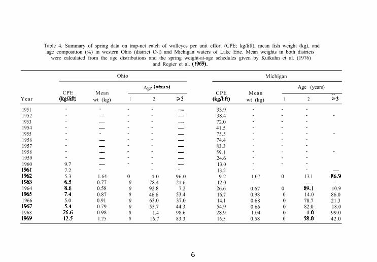
Table 4. Summary of spring data on trap-net catch of walleyes per unit effort (CPE; kg/lift), mean fish weight (kg), andage composition (%) in western Ohio (district O-l) and Michigan waters of Lake Erie. Mean weights in both districts

were calculated from the age distributions and the spring weight-at-age schedules given by Kutkuhn et al. (1976)and Regier et al. (1%9).

YearCPE

&dW

Ohio Michigan

Age (ye=@ Age (years)Mean CPE Mean

wt (kg) 1 2 $3 (kg/W wt (kg) 1 2 53

1951195219531954195519561957195819591960l%l1%21%319641%519661%719681%9

- - - - 33.938.472.041.575.574.483.359.124.613.013.29.2

12.026.616.714.154.928.916.5

- - -- - - -

-- --

- - - - -- - - - - -

-- - - --

- --- - - - -- - - - - -- - - -

-- --

- - - - -9.77.25.3

- - - - --

1.640.770.580.870.910.790.981.25

-96.021.6

00000000

-4.0

78.492.846.663.055.7

1.416.7

0

000000

-13.1

89-l14.078.782.0

8;9-

10.986.021.318.099.042.0

-1.07-

0.670.980.680.661.040.58

5.0

7.253.437.044.398.683.3

same period. Therefore we concluded that, where necessary, data onmean weights and age distributions collected in Ohio could be used withCPE data from both Ohio and Michigan in deriving indices of stock abun-dance. This adjustment enabled us to derive separate sets of abundanceindices for age groups I through IV, and for all age groups combined, fromthe Ohio data for 1948-69 and the Michigan data for 1946-69.

Annual survival rates

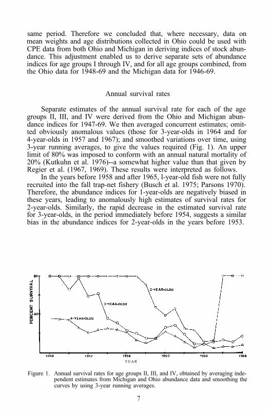
Separate estimates of the annual survival rate for each of the agegroups II, III, and IV were derived from the Ohio and Michigan abun-dance indices for 1947-69. We then averaged concurrent estimates; omit-ted obviously anomalous values (those for 3-year-olds in 1964 and for4-year-olds in 1957 and 1967); and smoothed variations over time, using3-year running averages, to give the values required (Fig. 1). An upperlimit of 80% was imposed to conform with an annual natural mortality of20% (Kutkuhn et al. 1976)--a somewhat higher value than that given byRegier et al. (1967, 1969). These results were interpreted as follows.

In the years before 1958 and after 1965, l-year-old fish were not fullyrecruited into the fall trap-net fishery (Busch et al. 1975; Parsons 1970).Therefore, the abundance indices for 1-year-olds are negatively biased inthese years, leading to anomalously high estimates of survival rates for2-year-olds. Similarly, the rapid decrease in the estimated survival ratefor 3-year-olds, in the period immediately before 1954, suggests a similarbias in the abundance indices for 2-year-olds in the years before 1953.

YEAR

Figure 1. Annual survival rates for age groups II, III, and IV, obtained by averaging inde-pendent estimates from Michigan and Ohio abundance data and smoothing thecurves by using 3-year running averages.

7

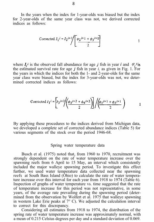
In the years when the index for 1-year-olds was biased but the indexfor 2-year-olds of the same year class was not, we derived correctedindices as follows:

where $i is the observed fall abundance for age j fish in year i and @i iisthe estimated survival rate for age j fish in year i, as given in Fig. 1. Forthe years in which the indices for both the 1- and 2-year-olds for the sameyear class were biased, but the index for 3-year-olds was not, we deter-mined corrected indices as follows:

By applying these procedures to the indices derived from Michigan data,we developed a complete set of corrected abundance indices (Table 5) forvarious segments of the stock over the period 1946-68.

Spring water temperature data

Busch et al. (1975) noted that, from 1960 to 1970, recruitment wasstrongly dependent on the rate of water temperature increase over thespawning reefs from 6 April to 15 May, an interval which consistentlyincluded the major walleye spawning period. To investigate this effectfurther, we used water temperature data collected near the spawningreefs at South Bass Island (Ohio) to calculate the rate of water tempera-ture increase over this interval for each year from 1918 to 1974 (Table 6).Inspection of graphs of water temperature vs. time suggested that the rateof temperature increase for this period was not representative, in someyears, of the average rate prevailing during the spawning period (deter-mined from the observation by Wolfert et al. 1975 that walleye spawningin western Lake Erie peaks at 7° C). We adjusted the calculation intervalto correct for this discrepancy.

Considering all estimates from 1918 to 1974, the distribution of thespring rate of water temperature increase was approximately normal, witha mean of 0.215 Celsius degrees per day and a standard deviation of 0.069.

8

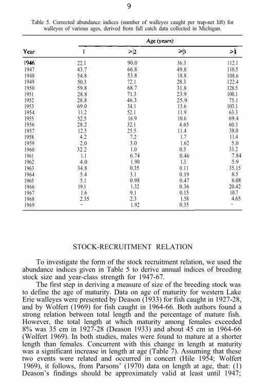
Table 5. Corrected abundance indices (number of walleyes caught per trap-net lift) forwalleyes of various ages, derived from fall catch data collected in Michigan.

19471948194919501951195219531954195519561957195819591960196119621963196419651966196719681969

22.143.754.850.359.828.828.869.011.252.528.212.54.22.0

32.21.14.0

34.85.45.1

19.11.62.35-

90.0 36.366.8 49.853.8 18.872.1 28.368.7 31.871.3 23.946.3 25.934.1 13.652.1 11.916.9 10.632.1 4.6525.5 11.47.2 1.73.0 1.621.0 0.36.74 0.461.90 1.30.35 0.113.1 0.190.98 0.471.32 0.369.1 0.152.3 1.581.92 0.35

112.1110.5108.6122.4128.5100.175.1

103.163.369.460.338.011.45.0

33.27.845.9

35.158.56.08

20.4210.74.65-

STOCK-RECRUITMENT RELATION

To investigate the form of the stock recruitment relation, we used theabundance indices given in Table 5 to derive annual indices of breedingstock size and year-class strength for 1947-67.

The first step in deriving a measure of size of the breeding stock wasto define the age of maturity. Data on age of maturity for western LakeErie walleyes were presented by Deason (1933) for fish caught in 1927-28,and by Wolfert (1969) for fish caught in 1964-66. Both authors found astrong relation between total length and the percentage of mature fish.However, the total length at which maturity among females exceeded8% was 35 cm in 1927-28 (Deason 1933) and about 45 cm in 1964-66(Wolfert 1969). In both studies, males were found to mature at a shorterlength than females. Concurrent with this change in length at maturitywas a significant increase in length at age (Table 7). Assuming that thesetwo events were related and occurred in concert (Hile 1954; Wolfert1969), it follows, from Parsons’ (1970) data on length at age, that: (1)Deason’s findings should be approximately valid at least until 1947;

9

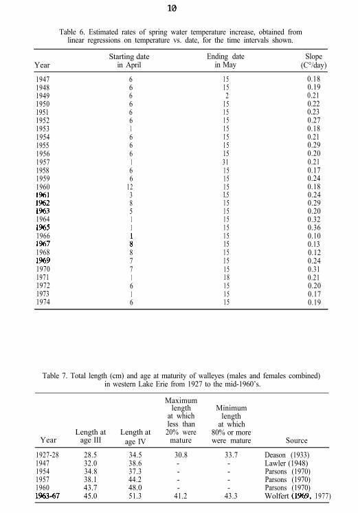
Table 6. Estimated rates of spring water temperature increase, obtained fromlinear regressions on temperature vs. date, for the time intervals shown.

YearStarting date Ending date Slope

in April in May (C°/day)

194719481949195019511952195319541955195619571958195919601%1I%21%319641%519661%719681%919701971197219731974

6666661666166

1238511

A8771616

15 0.1815 0.192 0.21

15 0.2215 0.2315 0.2715 0.1815 0.2115 0.2915 0.2031 0.2115 0.1715 0.2415 0.18I.5 0.2415 0.2915 0.2015 0.3215 0.3615 0.1015 0.1315 0.1215 0.2415 0.3118 0.2115 0.2015 0.1715 0.19

Table 7. Total length (cm) and age at maturity of walleyes (males and females combined)in western Lake Erie from 1927 to the mid-1960’s.

Year

1927-2819471954195719601%3-67

Maximumlength Minimum

at which lengthless than at which

Length at Length at 20% were 80% or moreage III age IV mature were mature Source

28.5 34.5 30.8 33.7 Deason (1933)32.0 38.6 - - Lawler (1948)34.8 37.3 - - Parsons (1970)38.1 44.2 - - Parsons (1970)43.7 48.0 - - Parsons (1970)45.0 51.3 41.2 43.3 Wolfert (1%9, 1977)

10

Lawler’s (1948) data on length at age then imply that in 1947 40% of the3-year-old, and all of the 4-year-old and older, fish were mature; and (2)Deason’s length-maturity relation indicates that most fish aged 3 and overwere mature from 1954 on, and Wolfert’s length-maturity relation indi-cates that most fish aged 3 and over were mature from 1960 on. In theabsence of information on the exact manner in which length at maturitychanged over the critical period from 1947 to 1960, we made the followingassumptions in deriving indices of abundance for mature fish: (1) in 1946-69, all fish 4 years old and older were mature; (2) in 1946-47, 40% of the3-year-olds were mature; (3) in 1954-67, 100% of the 3-year-olds weremature; and (4) from 1948 to 1953, the percentage of mature 3-year-oldsincreased linearly.

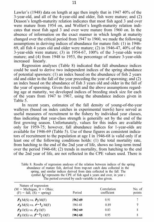
Regression analyses (Table 8) indicated that fall abundance indicescould be used to derive two independent indices of the spring abundanceof potential spawners: (1) an index based on the abundance of fish 2 yearsold and older in the fall of the year preceding the year of spawning; and (2)an index based on the abundance of fish 3 years old and older in the fall ofthe year of spawning. Given this result and the above assumptions regard-ing age at maturity, we developed indices of breeding stock size for eachof the years from 1947 to 1967, using the abundance indices given inTable 5.

In recent years, estimates of the fall density of young-of-the-yearwalleyes (based on index catches in experimental trawls) have served asuseful measures of recruitment to the fishery by individual year classes,thus indicating that year-class strength is generally set by the end of thefirst growing season. Unfortunately, values for this index are availableonly for 1959-75; however, fall abundance indices for 1-year-olds areavailable for 1946-69 (Table 5). Use of these figures as consistent indica-tors of recruitment to the population at age I in 1946-68 is valid only if atleast one of the following conditions holds: (1) the total mortality rate,from hatching to the end of the 2nd year of life, shows no long-term trendover the period 1946-68; (2) trends in mortality, from hatching to the endof the 2nd year of life, are not reflected in the CPE values used. There is

Table 8. Results of regression analyses of the relation between indices of the springabundance of mature fish, derived from trap-net catch data collected in the

spring, and similar indices derived from data collected in the fall. Thesymbol I,@ represents the CPE of fish aged k years and over, in year i.

The period covered by each variable is also given.

Nature of regression(M = Michigan, 0 = Ohio;

(F) = fall, (S) = spring) PeriodCorrelation No. ofcoefficient points

1’3 M(S) vs. I’3 M(F) 1%2-69 0.91 7

1’3 M(S) vs. j-12 M(F) 1961-68 0.89 I

$3 O(S) vs. $3 O(F) 1%2-69 0.83 8

li3 O(S) vs. g-12 O(F) 1%1-68 0.95 8

11

no direct evidence of a long-term trend in the natural mortality rate ofyoung fish. Fishing pressure on young-of-the-year walleyes has alwaysbeen negligible or lacking (Busch et al. 1975; Parsons 1970; Regier et al.1969). However, fishing pressure on 1-year-olds increased significantlybecause of the introduction and widespread use of gillnets of small andintermediate mesh size, primarily in Canadian waters, and because of theincrease in growth rate, which made yearlings increasingly vulnerable tothe fall trap-net fishery (Busch et al. 1975; Parsons 1970; Regier et al.1969). For these changes in the fishing mortality rate of 1-year-olds to bestrongly reflected in the fall CPE data from Michigan, extensive move-ment of 1-year-olds from Canadian to Michigan waters during the springand summer of each year would be required. The tagging studies of Fer-guson and Derksen (1971) and Wolfert (1963) showed, however, that suchmovement of yearlings did not occur. Therefore, we concluded that theknown trends in the overall mortality rate for young fish in this populationwere probably not strongly reflected in the fall abundance indices for1-year-olds derived from Michigan catches, and that these figures couldserve as a consistent index of recruitment to the population at age I in1946-68. The high correlation of this index with both the index catches foryoung-of-the-year (r = 0.89 for year-classes 1959 to 1%7), and Parsons’(1970) virtual population estimates of year-class strength (r = 0.863 foryear classes 1945 to l%l), provides empirical support for these conclu-sions.

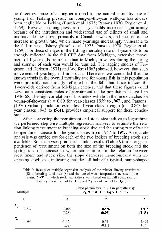
After converting the recruitment and stock size indices to logarithms,we performed step-wise multiple regression analyses to estimate the rela-tion linking recruitment to breeding stock size and the spring rate of watertemperature increase for the year classes from 1947 to 1%7. A separateanalysis was carried out for each of the two indices of breeding stock sizeavailable. Both analyses produced similar results (Table 9): a strong de-pendence of recruitment on both the size of the breeding stock and thespring rate of increase in water temperature. In the relation betweenrecruitment and stock size, the slope decreases monotonically with in-creasing stock size, indicating that the left half of a typical, hump-shaped

Table 9. Results of multiple regression analyses of the relation linking recruitment(R) to breeding stock size (S) and the rate of water temperature increase in thespring (iAT), in which stock size indices were based on the fall abundance of

fish 3 years old and older (Z3+) and 2 years old and older (Z2+)

MultipleFitted parameters ( f SD in parentheses):

r a P s

I3+ 0.837 0.009(0.28)

z2+0.804 -0.42 0.53 4.422

(0.32) (0.11) (1.35)

12

stock-recruitment curve is involved. The temperature effect is multiplica-tive and independent of stock size, and thus in accord with Kicker’s (1975)general analysis of the probable effects of physical environmental factorson recruitment.

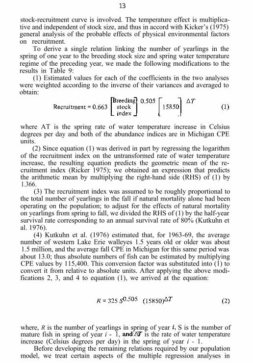
To derive a single relation linking the number of yearlings in thespring of one year to the breeding stock size and spring water temperatureregime of the preceding year, we made the following modifications to theresults in Table 9:

(1) Estimated values for each of the coefficients in the two analyseswere weighted according to the inverse of their variances and averaged toobtain:

where AT is the spring rate of water temperature increase in Celsiusdegrees per day and both of the abundance indices are in Michigan CPEunits.

(2) Since equation (1) was derived in part by regressing the logarithmof the recruitment index on the untransformed rate of water temperatureincrease, the resulting equation predicts the geometric mean of the re-cruitment index (Ricker 1975); we obtained an expression that predictsthe arithmetic mean by multiplying the right-hand side (RHS) of (1) by1.366.

(3) The recruitment index was assumed to be roughly proportional tothe total number of yearlings in the fall if natural mortality alone had beenoperating on the population; to adjust for the effects of natural mortalityon yearlings from spring to fall, we divided the RHS of (1) by the half-yearsurvival rate corresponding to an annual survival rate of 80% (Kutkuhn etal. 1976).

(4) Kutkuhn et al. (1976) estimated that, for 1963-69, the averagenumber of western Lake Erie walleyes 1.5 years old or older was about1.5 million, and the average fall CPE in Michigan for this same period wasabout 13.0; thus absolute numbers of fish can be estimated by multiplyingCPE values by 115,400. This conversion factor was substituted into (1) toconvert it from relative to absolute units. After applying the above modi-fications 2, 3, and 4 to equation (1), we arrived at the equation:

where, R is the number of yearlings in spring of year i, S is the number ofmature fish in spring of year i - 1, and!@ is the rate of water temperatureincrease (Celsius degrees per day) in the spring of year i - 1.

Before developing the remaining relations required by our populationmodel, we treat certain aspects of the multiple regression analyses in

13

more detail. There are similar secular trends in the data for both stock sizeand recruitment. Therefore the strong correlation between these twovariables may not stem from a causal connection, but rather from theaction of some additional factor(s), such as fishing or increased naturalmortality, operating to reduce both stock size and recruitment over aboutthe same period. This possibility cannot be definitively rejected on thebasis of the available data. However, the following results provide addi-tional support for the causal interpretation.

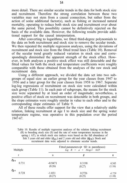
After converting to logarithms, we fitted third-degree polynomials tothe data on both recruitment and stock size to remove the secular trends.We then repeated the multiple regression analyses, using the deviations ofrecruitment and stock size from the fitted trend lines (Table 10). Removalof the secular trend greatly reduced variation in stock size and corre-spondingly diminished the apparent strength of the stock effect. How-ever, in both analyses a positive stock effect was still detectable and thefitted values for both the stock and temperature coefficients were roughlycomparable with those obtained from the analyses of the raw stock andrecruitment data.

Using a different approach, we divided the data set into two sub-groups of equal size: an earlier group for the year classes from 1947 to1956 and a later group for the year classes from 1958 to 1967. Separatelog-log regressions of recruitment on stock size were calculated withineach group (Table 11). In each pair of subgroups, the means for the stocksize were separated by at least an order of magnitude; nevertheless, apositive effect of stock on recruitment was detectable in both groups, andthe slope estimates were roughly similar in value to each other and to thecorresponding slope estimates of Table 9.

All of these results offer support for the view that a relatively stablerelation, linking recruitment at age I to stock size and the spring watertemperature regime, was operative in this population over the period1947-67.

Table 10. Results of multiple regression analyses of the relation linking recruitment(R) to breeding stock size (S) and the rate of water temperature increase in thespring ( AT), in which stock size indices were based on the fall abundance of

fish 3 years old and older (Z3+) and 2 years old and older (Z2+). Stock andrecruitment data were adjusted to eliminate secular trends.

MultipleFitted parameters (i* SD in parentheses):

log R = a + 8logs+ 6AT

r a P 6

Z3+0.731 -0.9471 0.3198 4.343

(0.26) (0.27) (1.16)

Z2+0.728 -1.031 0.2726

(0.27) (0.25)4.729

(1.10)

14

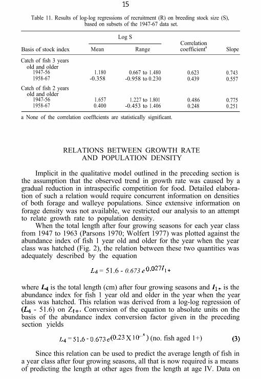
Table 11. Results of log-log regressions of recruitment (R) on breeding stock size (S),based on subsets of the 1947-67 data set.

Log SCorrelation

Basis of stock index Mean Range coefficienta Slope

Catch of fish 3 yearsold and older

1947-56 1.180 0.667 to 1.480 0.623 0.7431958-67 -0.358 -0.958 to 0.230 0.439 0.557

Catch of fish 2 yearsold and older

1947-56 1.657 1.227 to 1.801 0.486 0.7751958-67 0.400 -0.453 to 1.406 0.248 0.251

a None of the correlation coefftcients are statistically significant.

RELATIONS BETWEEN GROWTH RATEAND POPULATION DENSITY

Implicit in the qualitative model outlined in the preceding section isthe assumption that the observed trend in growth rate was caused by agradual reduction in intraspecific competition for food. Detailed elabora-tion of such a relation would require concurrent information on densitiesof both forage and walleye populations. Since extensive information onforage density was not available, we restricted our analysis to an attemptto relate growth rate to population density.

When the total length after four growing seasons for each year classfrom 1947 to 1963 (Parsons 1970; Wolfert 1977) was plotted against theabundance index of fish 1 year old and older for the year when the yearclass was hatched (Fig. 2), the relation between these two quantities wasadequately described by the equation

L4 = 51.6 - 0.673 ,o.02711+

where L4 is the total length (cm) after four growing seasons and It+ is theabundance index for fish 1 year old and older in the year when the yearclass was hatched. This relation was derived from a log-log regression of(L4 - 51.6) on ZI+. Conversion of the equation to absolute units on thebasis of the abundance index conversion factor given in the precedingsection yields

~~ = 51.6 - 0.673 ,(0.23 X lo-“) (no. fish aged 1+)

Since this relation can be used to predict the average length of fish ina year class after four growing seasons, all that is now required is a meansof predicting the length at other ages from the length at age IV. Data on

15

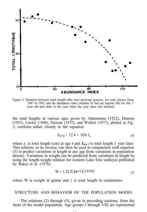
Figure 2. Relation between total length after four growing seasons, for year classes from1947 to 1963, and the abundance index (number of fish per trap-net lift) for fish 1year old and older in the year when the year class was hatched.

the total lengths at various ages given by Adamstone (1922), Deason(1933), Lawler (1948), Parsons (1972), and Wolfert (1977), plotted in Fig.3, conform rather closely to the equation

Lt+l = 12.4 + .836 Lt (4)

where Lt is total length (cm) at age c and Lt+l is total length 1 year later.This relation, or its inverse, can then be used in conjunction with equation(3) to predict variations in length at any age from variations in populationdensity. Variations in weight can be predicted from variations in length byusing the length-weight relation for western Lake Erie walleyes publishedby Baker et al. (1976)

W = 1.32 X lo-2 ~2.9302 (5)

where W is weight in grams and L is total length in centimeters.

STRUCTURE AND BEHAVIOR OF THE POPULATION MODEL

The relations (2) through (5), given in preceding sections, form theheart of the model population. Age groups I through VIII are represented

16

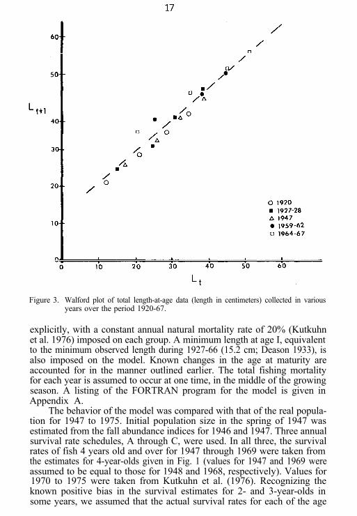
Figure 3. Walford plot of total length-at-age data (length in centimeters) collected in variousyears over the period 1920-67.

explicitly, with a constant annual natural mortality rate of 20% (Kutkuhnet al. 1976) imposed on each group. A minimum length at age I, equivalentto the minimum observed length during 1927-66 (15.2 cm; Deason 1933), isalso imposed on the model. Known changes in the age at maturity areaccounted for in the manner outlined earlier. The total fishing mortalityfor each year is assumed to occur at one time, in the middle of the growingseason. A listing of the FORTRAN program for the model is given inAppendix A.

The behavior of the model was compared with that of the real popula-tion for 1947 to 1975. Initial population size in the spring of 1947 wasestimated from the fall abundance indices for 1946 and 1947. Three annualsurvival rate schedules, A through C, were used. In all three, the survivalrates of fish 4 years old and over for 1947 through 1969 were taken fromthe estimates for 4-year-olds given in Fig. 1 (values for 1947 and 1969 wereassumed to be equal to those for 1948 and 1968, respectively). Values for1970 to 1975 were taken from Kutkuhn et al. (1976). Recognizing theknown positive bias in the survival estimates for 2- and 3-year-olds insome years, we assumed that the actual survival rates for each of the age

17

groups from I through III were bounded above by the estimates given forthe group in Fig. 1, and below by the estimates for fish 4 years old andolder. An upper bound of 80%, corresponding to the action of naturalmortality alone, was assigned to the survival rates for 1-year-olds. Ingeneral the values in schedule A were chosen from the upper regions oftheir respective ranges and the corresponding values in schedule B fromthe lower regions. A detailed description of the derivation of the survivalrates in each schedule is given in Table 12.

The simulated catches produced by schedules A and B bracket theobserved catches (Fig. 4). Under A, the simulated catch peaks later thanthe observed catch and then declines to an average level considerablyhigher than that observed. Under B, the simulated catch peaks earlier andat a lower level, and then declines to an average level only slightly higherthan that observed. These results suggest that, until the mid-1950’s, theschedule B survival rates are somewhat lower than those experienced bythe real population, whereas from the mid-1950’s to the end of the 1%0’s,the schedule A survival rates are somewhat higher.

Schedule C (Fig. 5) was constructed with this interpretation in mind.From 1947 to 1953, survival rates similar to those in schedule A are used.From 1954 to 1956, there is a transition to a set of rates similar to those inB, which then continue in effect until 1975. These trends in survival areconsistent with the following sequence of events: In the early 1950’s, anincrease in the use of small- and large-mesh gillnets, a decrease in theminimum size limit in Canadian waters, and a steady increase in growthrate led to a rapid increase in fishing mortality, particularly among theyounger fish (Busch et al. 1975; Regier et al. 1%9). Beginning in 1966,however, increases in minimum size limits (Busch et al. 1975) and theirenforcement (Regier et al. 1%9) led to a reduction in fishing mortalityamong these younger fish. This age-dependent differential in fishing mor-

Table 12. Derivation of survival rate schedules A and B for 1948-68 and 1970-75. Rates in1947 and 1969 are assumed to be equal to those in 1948 and 1968, respectively. Aj i and

&i z {represent the survival rates of age j fish in year i for schedules A and B.;represents the survival rate of age j fish in year i as given in Fig. 1; ZC

@i i

represents the average survival rate in year igiven by Kutkuhn et al. (1976).

Age group

Schedule A Schedule B

Period Derivation Period Derivation

IV-VIII 1948-681970-75

III 1948-531954-681970-75

II 1948-581959-651966-68; 1970-75

I 1948-68; 1970-75

~~ i= adi 1947-75hi=Ki

Bji = Aji

A3i = p$ t *Q/2 1947-75 B3i = A+Aji= @iA3'=K'A2i = ( e2i+ &3')/2 1947-65 B2i=&i

A2f= 0,2f 1964i-75 B.+ z&iA2f=(A3'+0.8)/2Al'= (A2'+0.8)/2 1945-65 Blf=A2!

1966-75 Bl'=Al'

18

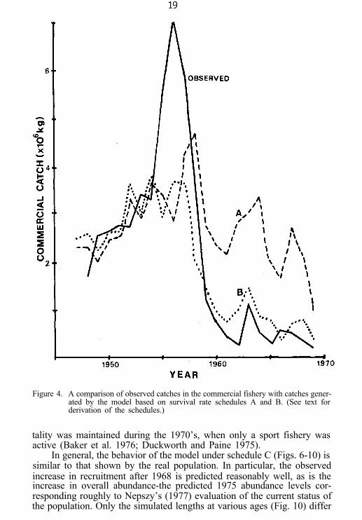
Figure 4. A comparison of observed catches in the commercial fishery with catches gener-ated by the model based on survival rate schedules A and B. (See text forderivation of the schedules.)

tality was maintained during the 1970’s, when only a sport fishery wasactive (Baker et al. 1976; Duckworth and Paine 1975).

In general, the behavior of the model under schedule C (Figs. 6-10) issimilar to that shown by the real population. In particular, the observedincrease in recruitment after 1968 is predicted reasonably well, as is theincrease in overall abundance-the predicted 1975 abundance levels cor-responding roughly to Nepszy’s (1977) evaluation of the current status ofthe population. Only the simulated lengths at various ages (Fig. 10) differ

19

Figure 5. Annual survival rates, by age groups, used in schedule C. (See text for derivationof the values.)

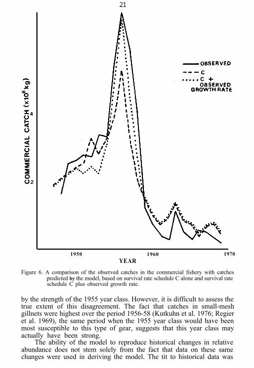
consistently from those observed. If the observed values for length at ageIV are imposed on the model rather than the values generated by equation(3), the simulated commercial catch follows a pattern almost identicalwith that observed (Fig. 6).

EVALUATION OF ANALYSES AND SIMULATION STUDIES

We have shown that the available information on relative abundance,year-class strength, and growth for western Lake Erie walleyes can beused to construct a quantitative version of the qualitative model outlinedin the introductory sections. We have also shown that a reasonable repre-sentation of the actual fishing mortality regime in 1947-75 elicits from thismodel a general pattern of behavior closely similar to that shown by thereal population. Furthermore, both the extent and rapidity of the recoveryin year-class strength and general abundance after 1968 are predicted withreasonable accuracy. Since the data used to derive the basic relations forthe model extended only to 1968, the continued correspondence betweenreal and predicted behavior beyond this date suggests that quantitativelysimilar relations were still operative in the population and that the modelhas true predictive capabilities.

Although the level of agreement between simulated and observedbehavior is reasonably high, it is not perfect. Perhaps the most significantdiscrepancy is in the strength of the 1955 year class: the model predictedthat it was very strong, whereas the observational index suggested that itwas only of moderate strength. This discrepancy is important because theheight of the peak in the simulated commercial catch is determined in part

20

1950 1960 1970YEAR

Figure 6. A comparison of the observed catches in the commercial fishery with catchespredicted by the model, based on survival rate schedule C alone and survival rateschedule C plus observed growth rate.

by the strength of the 1955 year class. However, it is difficult to assess thetrue extent of this disagreement. The fact that catches in small-meshgillnets were highest over the period 1956-58 (Kutkuhn et al. 1976; Regieret al. 1969), the same period when the 1955 year class would have beenmost susceptible to this type of gear, suggests that this year class mayactually have been strong.

The ability of the model to reproduce historical changes in relativeabundance does not stem solely from the fact that data on these samechanges were used in deriving the model. The tit to historical data was

21

41950 1960 1970

YEAR

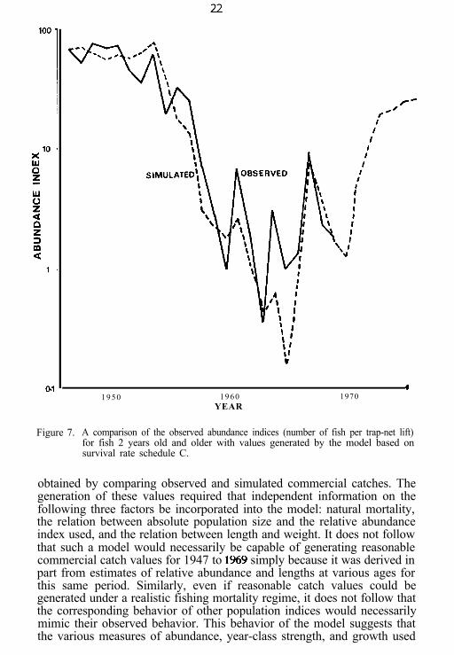
Figure 7. A comparison of the observed abundance indices (number of fish per trap-net lift)for fish 2 years old and older with values generated by the model based onsurvival rate schedule C.

obtained by comparing observed and simulated commercial catches. Thegeneration of these values required that independent information on thefollowing three factors be incorporated into the model: natural mortality,the relation between absolute population size and the relative abundanceindex used, and the relation between length and weight. It does not followthat such a model would necessarily be capable of generating reasonablecommercial catch values for 1947 to 1%9 simply because it was derived inpart from estimates of relative abundance and lengths at various ages forthis same period. Similarly, even if reasonable catch values could begenerated under a realistic fishing mortality regime, it does not follow thatthe corresponding behavior of other population indices would necessarilymimic their observed behavior. This behavior of the model suggests thatthe various measures of abundance, year-class strength, and growth used

22

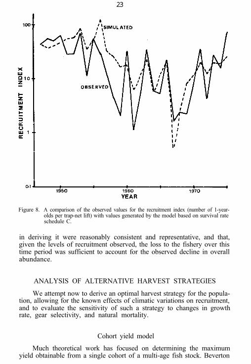
Figure 8. A comparison of the observed values for the recruitment index (number of 1-year-olds per trap-net lift) with values generated by the model based on survival rateschedule C.

in deriving it were reasonably consistent and representative, and that,given the levels of recruitment observed, the loss to the fishery over thistime period was sufficient to account for the observed decline in overallabundance.

ANALYSIS OF ALTERNATIVE HARVEST STRATEGIES

We attempt now to derive an optimal harvest strategy for the popula-tion, allowing for the known effects of climatic variations on recruitment,and to evaluate the sensitivity of such a strategy to changes in growthrate, gear selectivity, and natural mortality.

Cohort yield model

Much theoretical work has focused on determining the maximumyield obtainable from a single cohort of a multi-age fish stock. Beverton

23

Figure 9. A comparison of observed values, for the ratio of the abundance of 2-year-olds tothe abundance of fish 2 years old and older, with values generated by the modelbased on survival rate schedule C.

Figure 10. A comparison of observed lengths (solid line) at ages 3 and 4 with lengthsgenerated by the model based on survival rate schedule C (broken line).

24

and Holt (1957) showed that yield curves peak at low fishing mortalityrates when the natural mortality is low. At high natural mortality ratesthese peaks disappear, and maximum yields are then obtained at highfishing mortality rates. Thus, a strategy to maximize yield from a cohortwill be sensitive to estimates of natural mortality.

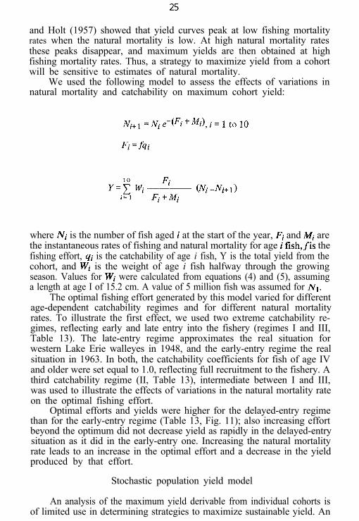
We used the following model to assess the effects of variations innatural mortality and catchability on maximum cohort yield:

where Ni is the number of fish aged i at the start of the year, Fi and Mi arethe instantaneous rates of fishing and natural mortality for age i fish,fis thefishing effort, qi is the catchability of age i fish, Y is the total yield from thecohort, and Wi is the weight of age i fish halfway through the growingseason. Values for Wi were calculated from equations (4) and (5), assuminga length at age I of 15.2 cm. A value of 5 million fish was assumed for N1.

The optimal fishing effort generated by this model varied for differentage-dependent catchability regimes and for different natural mortalityrates. To illustrate the first effect, we used two extreme catchability re-gimes, reflecting early and late entry into the fishery (regimes I and III,Table 13). The late-entry regime approximates the real situation forwestern Lake Erie walleyes in 1948, and the early-entry regime the realsituation in 1963. In both, the catchability coefficients for fish of age IVand older were set equal to 1.0, reflecting full recruitment to the fishery. Athird catchability regime (II, Table 13), intermediate between I and III,was used to illustrate the effects of variations in the natural mortality rateon the optimal fishing effort.

Optimal efforts and yields were higher for the delayed-entry regimethan for the early-entry regime (Table 13, Fig. 11); also increasing effortbeyond the optimum did not decrease yield as rapidly in the delayed-entrysituation as it did in the early-entry one. Increasing the natural mortalityrate leads to an increase in the optimal effort and a decrease in the yieldproduced by that effort.

Stochastic population yield model

An analysis of the maximum yield derivable from individual cohorts isof limited use in determining strategies to maximize sustainable yield. An

25

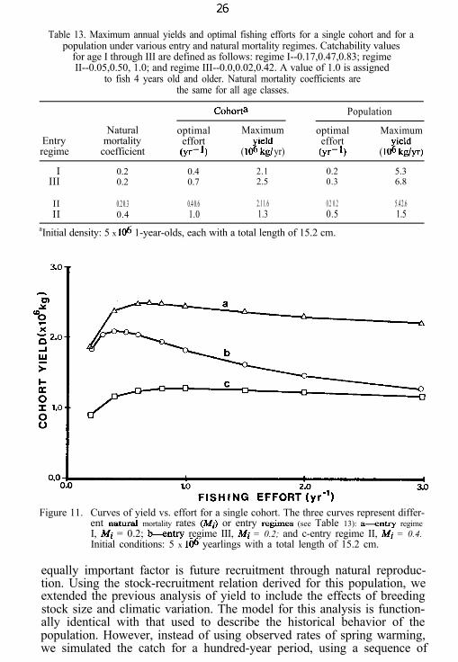
Table 13. Maximum annual yields and optimal fishing efforts for a single cohort and for apopulation under various entry and natural mortality regimes. Catchability values

for age I through III are defined as follows: regime I--0.17,0.47,0.83; regimeII--0.05,0.50, 1.0; and regime III--0.0,0.02,0.42. A value of 1.0 is assigned

to fish 4 years old and older. Natural mortality coefficients arethe same for all age classes.

Cohorta Population

Natural optimal Maximum optimal MaximumEntry mortality effort effortregime coefficient (yr- 9 ( IOK: yr) (yr- 4 ( 1OK~yr)

I 0.2 0.4 2.1 0.2 5.3III 0.2 0.7 2.5 0.3 6.8

II 0.2 0.3 0.4 0.6 2.1 1.6 0.2 0.2 5.4 2.6II 0.4 1.0 1.3 0.5 1.5

aInitial density: 5 x 106 1-year-olds, each with a total length of 15.2 cm.

Figure 11. Curves of yield vs. effort for a single cohort. The three curves represent differ-ent natullrl mortality rates (Mi) or entry ~&IIIIZS (see Table 13): -ntry regimeI, Mi = 0.2; &ntry regime III, Mi = 0.2; and c-entry regime II, Mi = 0.4.Initial conditions: 5 x 106 yearlings with a total length of 15.2 cm.

equally important factor is future recruitment through natural reproduc-tion. Using the stock-recruitment relation derived for this population, weextended the previous analysis of yield to include the effects of breedingstock size and climatic variation. The model for this analysis is function-ally identical with that used to describe the historical behavior of thepopulation. However, instead of using observed rates of spring warming,we simulated the catch for a hundred-year period, using a sequence of

26

warming rates drawn at random from the empirically determined proba-bility distribution for that quantity.

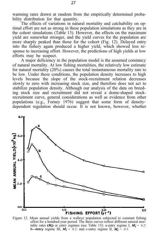
The effects of variations in natural mortality and catchability on op-timal effort are not as strong in these population simulations as they are inthe cohort simulations (Table 13). However, the effects on the maximumyield are somewhat stronger, and the yield curves for the population aremore sharply peaked than those for the cohort (Fig. 12). Delayed entryinto the fishery again produced a higher yield, which showed less re-sponse to increasing effort. However, the predictions of high yields at lowefforts may be suspect.

A major deficiency in the population model is the assumed constancyof natural mortality. At low fishing mortalities, the relatively low estimatefor natural mortality (20%) causes the total instantaneous mortality rate tobe low. Under these conditions, the population density increases to highlevels because the slope of the stock-recruitment relation decreasesslowly to zero with increasing stock size, and therefore does not act tostabilize population density. Although our analysis of the data on breed-ing stock size and recruitment did not reveal a dome-shaped stock-recruitment curve, general considerations as well as evidence from otherpopulations (e.g., Forney 1976) suggest that some form of density-dependent regulation should occur. It is not known, however, whether

Figure 12. Mean annual yields from a walleye population subjected to constant fishingeffort for a hundred-year period. The three curves reflect different natural mor-tality rates (Mi) or entry regimes (see Table 13): a-entry regime I, Mi = 0.2;kntry regime III, Mi = 0.2; and c-entry regime II, Mi = 0.3.

27

this regulation will be reflected in the natural mortality rates of yearlingand older fish or in the mortality of eggs, larvae, and juveniles. Withoutthis information, one cannot place much confidence in the high meanannual yields predicted for relatively low levels of fishing effort. A greaterdegree of reliability can be attached to the general pattern of responseexhibited by the optimal fishing effort to the kinds of changes in thecharacter of the fishery explored in these simulation studies.

Stochastic dynamic programming analysis

Another approach for estimating the maximum sustainable yield ofwalleyes in western Lake Erie is to determine the balance between yieldand future recruitment from the cohort. A technique to evaluate optimalfishing effort in this way can be derived from the principles of stochasticdynamic programming (Walters 1975). This technique allows the develop-ment of management strategies based on standing stock, or some othermeasure of population density, and a particular management objective(e.g., maximum sustainable yield or minimum variation in catch). Thedynamic programming approach applied to fisheries by Walters (1975)was designed for populations with nonoverlapping generations. Sincewalleyes do not conform to this assumption, we used a modified versionof Walters’ approach.

Instead of focusing on the total stock, we determined the optimaleffort for exploiting a cohort throughout the time it is in the population.This was done by assigning to each cohort, of a given size at age I, anumerical value equal to the total yield derived from that cohort plus themean annual value of the offspring of that cohort. The degree of fishingeffort that maximized this value was defined as the optimal effort. Thevalue of the offspring was determined from their number by a recursionprocess described by Walters (1975). The number of offspring was a func-tion of the number of reproducing adults in the cohort and the rate ofspring warming. A stochastic element was introduced into this scheme bydefining the spring warming rate in terms of its empirically determinedprobability distribution. The model which forms an essential part of thisanalysis was based on the cohort yield model described above and thestock-recruitment relation. A listing of the FORTRAN program for thismodel is given in Appendix B. Index catch values for young-of-the-yearwere used as indicators of numerical abundance at age I. Recruitment tothe fishery was defined by the moderate-entry regime described earlier(regime II, Table 13). A constant annual natural mortality rate was as-sumed for all age groups.

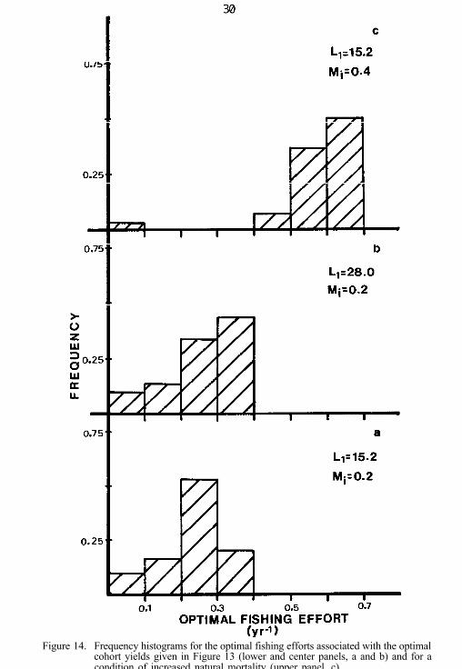
This approach yielded an optimal control law for the fishery definedin terms of the optimum harvest appropriate to a year class whosestrength was characterized by a particular value for young-of-the-year(Fig. 13). The range of fishing effort required to implement this law overthe range of such index values considered was given in terms of a fre-quency distribution (Fig. 14).

28

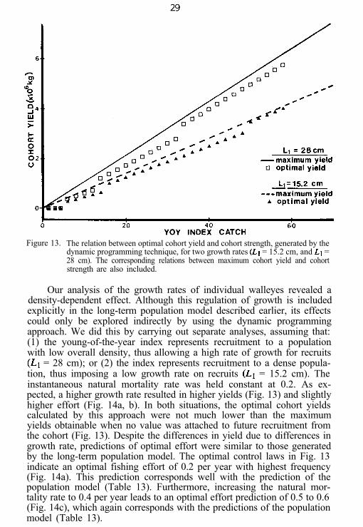
Figure 13. The relation between optimal cohort yield and cohort strength, generated by thedynamic programming technique, for two growth rates (Ll = 15.2 cm, and Ll =28 cm). The corresponding relations between maximum cohort yield and cohortstrength are also included.

Our analysis of the growth rates of individual walleyes revealed adensity-dependent effect. Although this regulation of growth is includedexplicitly in the long-term population model described earlier, its effectscould only be explored indirectly by using the dynamic programmingapproach. We did this by carrying out separate analyses, assuming that:(1) the young-of-the-year index represents recruitment to a populationwith low overall density, thus allowing a high rate of growth for recruits(Ll = 28 cm); or (2) the index represents recruitment to a dense popula-tion, thus imposing a low growth rate on recruits (Ll = 15.2 cm). Theinstantaneous natural mortality rate was held constant at 0.2. As ex-pected, a higher growth rate resulted in higher yields (Fig. 13) and slightlyhigher effort (Fig. 14a, b). In both situations, the optimal cohort yieldscalculated by this approach were not much lower than the maximumyields obtainable when no value was attached to future recruitment fromthe cohort (Fig. 13). Despite the differences in yield due to differences ingrowth rate, predictions of optimal effort were similar to those generatedby the long-term population model. The optimal control laws in Fig. 13indicate an optimal fishing effort of 0.2 per year with highest frequency(Fig. 14a). This prediction corresponds well with the prediction of thepopulation model (Table 13). Furthermore, increasing the natural mor-tality rate to 0.4 per year leads to an optimal effort prediction of 0.5 to 0.6(Fig. 14c), which again corresponds with the predictions of the populationmodel (Table 13).

29

a

Figure 14. Frequency histograms for the optimal fishing efforts associated with the optimalcohort yields given in Figure 13 (lower and center panels, a and b) and for acondition of increased natural mortality (upper panel, c).

30

EVALUATION OF OPTIMAL HARVEST STRATEGIES

The similarity of the predictions of optimal effort generated by thetwo models that consider both yield and future recruitment suggests that amore efficient management policy could be developed for the exploitationof walleyes in western Lake Erie. However, the magnitude of the result-ing catches is beyond existing predictive capability. The optimal catchesgenerated by these models probably overestimate the optimal catchesactually obtainable. This overestimation is due in part to our inability todefine the effects of high population densities on the mortality rates oper-ative at various life stages. For the same reason, it is not certain that theactual yield vs. effort curve would exhibit the sharp peak at low fishingefforts which was characteristic of the curves generated by our models. Abroad dome in this curve would allow a fairly wide range of fishing effortwithout major differences in yield.

Nevertheless, both models indicate optimal instantaneous fishingmortality rates of 0.2 to 0.3 per year, assuming a value of 0.2 for thenatural mortality rate. Even at higher natural mortality rates, the optimalfishing mortality rate does not increase beyond 0.6 per year. These figuresare in sharp contrast to those obtained from the estimated survival rates inFig. 1. Assuming a natural mortality rate of 0.2, the fishing mortality ratesfor fully recruited age groups range from 0.7 in 1948 to 2.8 in the mid-1960’s-values that indicate that this population has long been exploitedat levels beyond the optimum.

The simulation results also demonstrate that a catchability regimethat emphasizes delayed entry into the fishery yields greater harvests,which are less sensitive to supra-optimal exploitation, than does a regimewhich allows early entry.

CONCLUSIONS

Analysis of the data made available to us suggests that greatly in-creased exploitation of western Lake Erie walleyes during the 1950’s and1%0’s reduced population abundance to very low levels over a relativelyshort time. Data collected during this period appear to contain extractableinformation on the relations linking year-class strength to breeding stocksize and the spring water temperature regime, as well as on the relationlinking growth rate to population density. A model based on preliminaryestimates of these relations was relatively successful in accounting for theknown behavior of the population and was readily adaptable for use as amanagement tool. It may be possible to extend and refine this modelsufficiently for use in developing realistic management policies for thepopulation.

A C K N O W L E D G M E N T S

This study was funded by the Great Lakes Fishery Commission, theNational Research Council of Canada, the University of Toronto, and

31

Case Western Reserve University. We were assisted in our work by W. J.Christie, F. E. J. Fry, W. L. Hartman, J. Kutkuhn, J. H. Leach, S. J.Nepszy, and R. Scholl.

REFERENCES

ADAMSTONE, F. B.1922. Rates of growth of the blue and yellow pike perch. Univ. Toronto Studies 20, Publ.

Ont. Fish. Res. Lab. 5:77-86.ANONYMOUS.

1%1. Water temperatures at Put-In-Bay, Ohio from 1918. Ohio Dep. Nat. Resour. Tech.Rep. No. N-189. 36 pp.

BAKER, C. T., J. P. MUELLER, and D. L. JOHNSON.1976. Performance report: Lake Erie fishery research, Project F-35-R-14, Study III, Job

III-a. Ohio Department of Natural Resources, Columbus. 62 pp.BEVERTON, R. J. H., and S. J. HOLT.

1957. On the dynamics of exploited fish populations. U.K. Mm. Agric. Fish., Fish.Invest. (Ser. 2) 19. 533 pp.

BUSCH, W. N., R. L. SCHOLL, and W. L. HARTMAN.1975. Environmental factors affecting the strength of walleye year classes in Western

Lake Erie, 1960-1970. J. Fish. Res. Board Can. 32:1733-1743.DEASON, H. J.

1933. Preliminary report on the growth rate, dominance, and maturity of the pike-perches (Stizosredion) of Lake Erie. Trans. Am. Fish. Soc. 63:348-360.

DUCKWORTH, G. A., and 3. R. PAINE.1975. Summer creel census in the Canadian waters of the western basin of Lake Erie,

1975. Lake Erie Fisheries Assessment Unit Report 1975-1. Ontario Ministry ofNatural Resources. 69 pp.

FERGUSON, R. G., and A. J. DERKSEN.1971. Migrations of adult and juvenile walleyes (Stizostedion vitreum vitreum) in south-

em Lake Huron, Lake St. Clair, Lake Erie, and connecting waters. J. Fish. Res.Board Can. 28: 1133-l 142.

FORNEY, J. L.1976. Year class formation in the walleye population of Oneida Lake, New York, 1966-

73. J. Fish. Res. Board Can. 33:783-792.HARTMAN, W. L.

1973. Effects of exploitation, environmental changes, and new species on the fish habi-tats and resources of Lake Erie. Great Lakes Fish. Comm. Tech. Rep. No. 22.43PP.

HILE, R.1954. Fluctuations in growth and year-class strength of the walleye in Saginaw Bay.

U.S. Fish Wildl. Serv., Fish. Bull. 56:7-59.KUTKUHN, J., W. HARTMAN, A. HOLDER. R. KENYON. S. KERR. A. LAMSA. S.

NEPSZY, M.-PATRIARCHE, k. SCHOLL, bi’. SHEPHERD; and G. SPANGLER.1976. First technical report of the Great Lakes Fishery Commission Scientific Protocol

Comittee on Interagency Management of the Walleye Resource of Western LakeErie. Great Lakes Fishery Commission, Ann Arbor, Mich. 31 pp.

LANGLOIS, T. H.1945. Water, fishes, and cropland management. Trans. North Am. Wildl. Conf. 10:190-

1%.LAWLER, G. H.

1948. Preliminary population studies of five species of Lake Erie fishes. M.S. Thesis.Univ. Western Ontario, London. 47 pp.

LEACH, J. H., and S. J. NEPSZY.1976. The fish community in Lake Erie. J. Fish. Res. Board Can. 33:622-638.

32

NEPSZY, S. J.1977. Changes in percid populations and species interactions in Lake Erie. J. Fish. Res.

Board Can. 34:1861-1868.PARSONS, J. W.

1970. Walleye fishery of Lake Erie in 194362 with emphasis on contributions of the1942-61 year-classes. J. Fish. Res. Board Can. 27:1475-1489.

PARSONS, J. W.1972. Life history and production of walleyes of the 1959 year-class in western Lake

Erie, 1959-62. Trans. Am. Fish. Soc. 101:655-661.REGIER, H. A., V. C. APPLEGATE, and R. A. RYDER.

1%9. The ecology and management of the walleye in western Lake Erie. Great LakesFish. Comm. Tech. Rep. No. 15. 101 pp.

REGIER. H. A.. V. C. APPLEGATE. H. D. VAN METER, D. R. WOLFERT, R. C.FERGUSON, R. A. RYDER, and J. MANZ.1%7. The ecology and management of walleye in western Lake Erie. Great Lakes Fish.

Comm. 178 pp. (Unpubl. manuscr., fded Univ. Toronto)RICKER, W. E.

1975. Commnation and interpretation of biological statistics of fish populations. Fish.Res. Board Can., Bull: No. 191. 382 pp.

SHUTER. B. J.. and J. F. KOONCE.1977. A dynamic model of the Western Lake Erie walleye (Stizostedion vitreum vitreum)

population. J. Fish. Res. Board Can. 34: 1972-1982.SMITH. S. H.. H. J. BUETTNER. and-R. HILE.

1%1. Fishery statistical districts of the Great Lakes. Great Lakes Fish. Comm. Tech.Rep. No. 2. 24 pp.

WALTERS, C. J.1975. Optimal harvest strategies for salmon in relation to environmental variability and

uncertain production parameters. J. Fish. Res. Board Can. 32: 1777-1784.WOLFERT, D. R.

1%3. The movements of walleyes tagged as yearlings in Lake Erie. Trans. Am. Fish.Soc. 92:414-420.

WOLFERT, D. R.1%9. Maturity and fecundity of walleyes from the Eastern and Western basins of Lake

Erie. J. Fish. Res. Board Can. 26:1877-1888.WOLFERT, D. R.

1977. Age and growth of the walleye in Lake Erie, 1963-1968. Trans. Am. Fish. Soc.106: 569-577.

WOLFERT, D. R., W. N. BUSCH, and C. T. BAKER.1975. Predation by fish on walleye eggs on a spawning reef in western Lake Erie 1%9-71.

Ohio J. Sci. 75: 118-125.

33

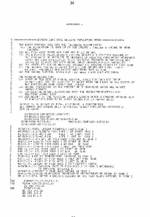
APPENDIX A

35

36

37

38

1

40