Division of Materials, Mechanics & Structures

Faculty of Engineering

Modeling the Structure-Permeability Relationship

for Woven Fabrics

Xueliang Xiao

Thesis submitted to The University of Nottingham

for the degree of Doctor of Philosophy

August 2012

i

CONTENTS

Abstract .............................................................................................................................. I

Acknowledgements ......................................................................................................... III

Nomenclature .................................................................................................................. IV

Glossary .......................................................................................................................... VI

Chapter 1 Introduction ...................................................................................................... 1

1.1 Background ............................................................................................................. 1

1.1.1 Definition of permeability ................................................................................ 1

1.1.2 Textile fabrics ................................................................................................... 3

1.2 Motivation ............................................................................................................... 6

1.3 Overview of thesis ................................................................................................... 8

Chapter 2 Literature review ............................................................................................ 10

2.1 Introduction ........................................................................................................... 10

2.2 Darcy flow in porous media .................................................................................. 11

2.3 Non-Darcy flow in porous media .......................................................................... 21

2.3.1 The Forchheimer equation in porous media ................................................... 22

2.3.2 Non-Darcy flow in converging-diverging channel ......................................... 27

2.4 Fabric deformation under uniform load ................................................................ 31

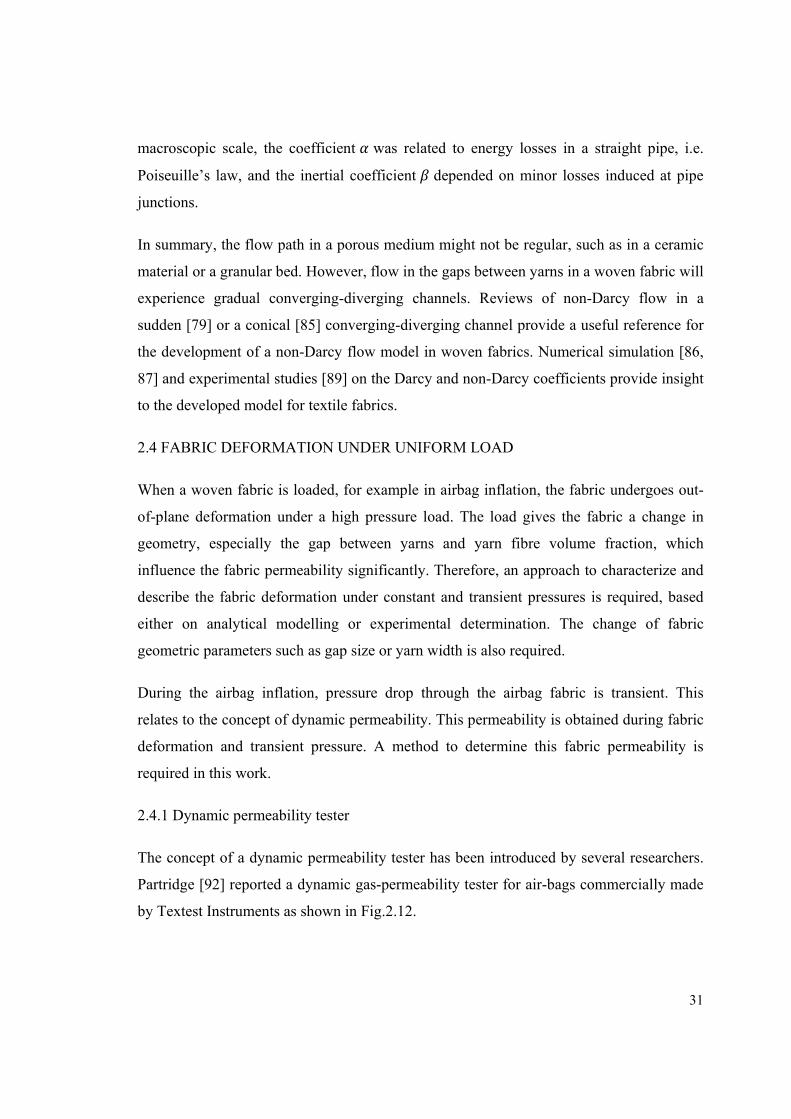
2.4.1 Dynamic permeability tester ........................................................................... 31

2.4.2 Mechanics of fabric deformation .................................................................... 33

2.5 Conclusions ........................................................................................................... 39

Chapter 3 Modelling of fabric static permeability .......................................................... 41

3.1 Intorduction ........................................................................................................... 41

ii

3.2 Static permeability of one-layer of woven fabric .................................................. 42

3.3 Analytical modelling of yarn and gap permeabilities ............................................ 44

3.3.1 Yarn permeability modelling .......................................................................... 44

3.3.2 Gap permeability modelling ........................................................................... 46

3.4 Verification by CFD simulation ............................................................................ 51

3.4.1 An introduction to the software packages....................................................... 52

3.4.2 Simulation for the Gebart model .................................................................... 56

3.4.3 Simulation for the gap permeability model .................................................... 58

3.5 Experimental verification ...................................................................................... 60

3.5.1 Loose fabric (Ф ≠ 0 in Eq.3.4) ...................................................................... 60

3.5.2 Tight fabric (Ф = 0 in Eq.3.4) ........................................................................ 68

3.6 Permeability modelling for 3D woven fabrics ...................................................... 70

3.6.1 Theoretical modeling ...................................................................................... 70

3.6.2 Experimental verification ............................................................................... 71

3.7 Conclusions ........................................................................................................... 76

Chapter 4 Analysis of fabric dynamic permeability ....................................................... 78

4.1 Introduction ........................................................................................................... 78

4.2 Experimental techniques ....................................................................................... 78

4.2.1 Design of the dynamic tester .......................................................................... 78

4.2.2 Experimental plan ........................................................................................... 79

4.3 Operating principle and data analysis.................................................................... 80

4.3.1 Operating principle of the dynamic permeability tester ................................. 80

4.3.2 Data analysis ................................................................................................... 81

4.4 Results and discussion ........................................................................................... 84

4.4.1 Temperature effects ........................................................................................ 84

iii

4.4.2 Static and dynamic permeability .................................................................... 85

4.4.3 Effect of initial pressure on the fabric permeability ....................................... 91

4.4.4 Effect of multiple fabric layers on the permeability ....................................... 92

4.5 Conclusions ........................................................................................................... 94

Chapter 5 Permeability modelling of deformed textiles under high pressure load ......... 95

5.1 Introduction ........................................................................................................... 95

5.2 Modelling of fabric deflection under high pressure load ...................................... 96

5.2.1 Development of analytical model ................................................................... 96

5.2.2 Experimental verification ............................................................................. 100

5.2.3 Results and discussion .................................................................................. 103

5.3 Modelling of fabric permeability under high pressure load ................................ 109

5.3.1 Development of the analytical model ........................................................... 109

5.3.2 Experimental verification ............................................................................. 112

5.3.3 Results and discussion .................................................................................. 112

5.4 Conclusions ......................................................................................................... 118

Chaper 6 Modelling of Non-Darcy flow in textiles ...................................................... 120

6.1 Introduction ......................................................................................................... 120

6.2 Analysis of Non-Darcy flow ............................................................................... 120

6.2.1 Hagen-Poiseuille flow in gradual converging-diverging channels ............... 120

6.2.2 Non-Darcy flow from Navier-Stokes Equation ............................................ 123

6.2.3 Analytical modelling of Non-Darcy flow ..................................................... 124

6.2.4 Hydraulic resistance of woven fabric ........................................................... 127

6.3 Verification by CFD simulations ........................................................................ 130

6.3.1 Non-Darcy flow observed by CFD simulations ........................................... 130

6.3.2 CFD simulations for GCD tubes ................................................................... 132

iv

6.3.3 CFD simulations for GCD plates .................................................................. 137

6.4 Validation ............................................................................................................ 140

6.4.1 Experimental verification ............................................................................. 140

6.4.2 Verification by published experimental data ................................................ 142

6.5 Non-Darcy flow model with fabric deformation ................................................. 143

6.6 Conclusions ......................................................................................................... 145

Chapter 7 Conclusions and future work ........................................................................ 147

7.1 Introduction ......................................................................................................... 147

7.2 General summary and conclusions ...................................................................... 147

7.3 Limitations and recommendations for future work ............................................. 152

7.3.1 Modelling limitations .................................................................................... 152

7.3.2 Recommendations for future work ............................................................... 154

References ..................................................................................................................... 156

Appendix I: Publications ............................................................................................... 167

Appendix II: Basic fluid mechanics .............................................................................. 168

Appendix III: Mechanics of plate deformation ............................................................. 177

Appendix IV: Derivation of the Gebart model and the Advani model ......................... 179

Appendix V: Measurement of shape factor for nine fabrics in Table 3-5 .................... 183

Appendix VI: Variation of streamlines in GCD flow channels with pressure .............. 186

Appendix VII: Analytical modelling for permeability of rectangular GCD gap .......... 190

I

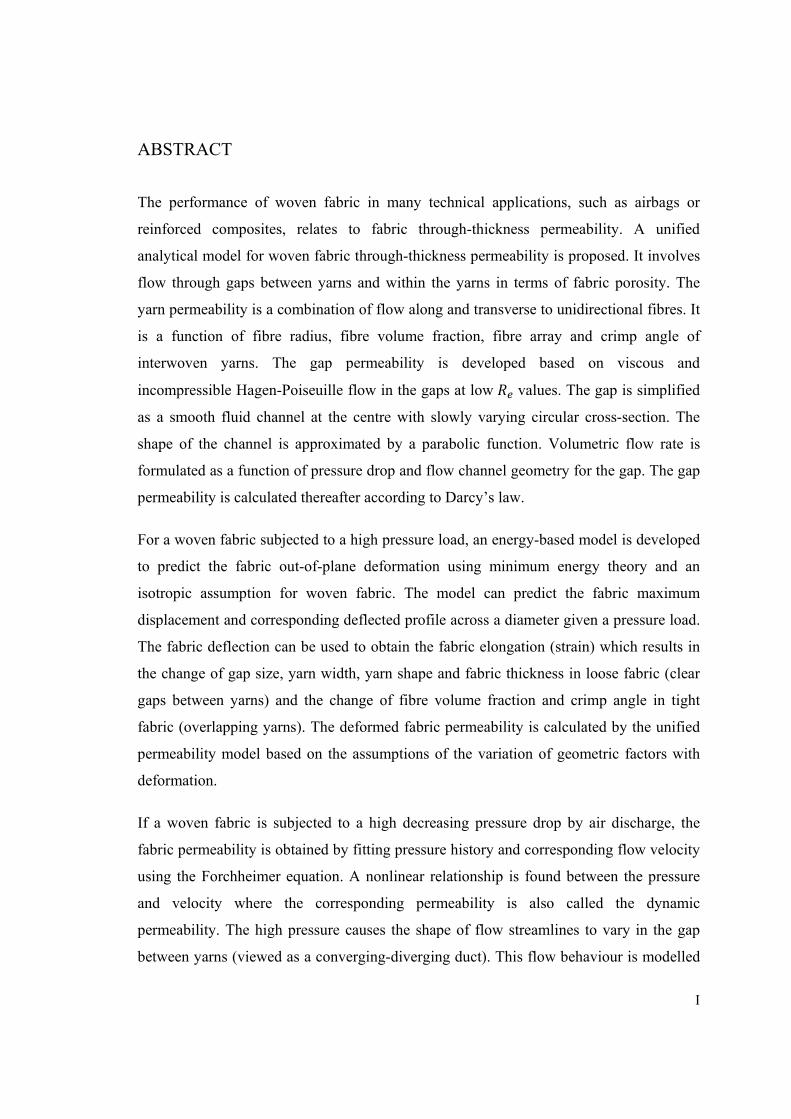
ABSTRACT

The performance of woven fabric in many technical applications, such as airbags or

reinforced composites, relates to fabric through-thickness permeability. A unified

analytical model for woven fabric through-thickness permeability is proposed. It involves

flow through gaps between yarns and within the yarns in terms of fabric porosity. The

yarn permeability is a combination of flow along and transverse to unidirectional fibres. It

is a function of fibre radius, fibre volume fraction, fibre array and crimp angle of

interwoven yarns. The gap permeability is developed based on viscous and

incompressible Hagen-Poiseuille flow in the gaps at low values. The gap is simplified

as a smooth fluid channel at the centre with slowly varying circular cross-section. The

shape of the channel is approximated by a parabolic function. Volumetric flow rate is

formulated as a function of pressure drop and flow channel geometry for the gap. The gap

permeability is calculated thereafter according to Darcy’s law.

For a woven fabric subjected to a high pressure load, an energy-based model is developed

to predict the fabric out-of-plane deformation using minimum energy theory and an

isotropic assumption for woven fabric. The model can predict the fabric maximum

displacement and corresponding deflected profile across a diameter given a pressure load.

The fabric deflection can be used to obtain the fabric elongation (strain) which results in

the change of gap size, yarn width, yarn shape and fabric thickness in loose fabric (clear

gaps between yarns) and the change of fibre volume fraction and crimp angle in tight

fabric (overlapping yarns). The deformed fabric permeability is calculated by the unified

permeability model based on the assumptions of the variation of geometric factors with

deformation.

If a woven fabric is subjected to a high decreasing pressure drop by air discharge, the

fabric permeability is obtained by fitting pressure history and corresponding flow velocity

using the Forchheimer equation. A nonlinear relationship is found between the pressure

and velocity where the corresponding permeability is also called the dynamic

permeability. The high pressure causes the shape of flow streamlines to vary in the gap

between yarns (viewed as a converging-diverging duct). This flow behaviour is modelled

II

by adding a non-Darcy term to Darcy’s law according to continuity theory and the

Bernoulli equation. Therefore, a predictive Forchheimer equation is given for flow

behaviour in a woven fabric based on the fabric geometry, structure and flow situation.

The developed analytical models were verified by CFD simulations and experiments in

this thesis. The comparisons showed good agreements. Sensitivity studies were conducted

to understand the effects of geometric factors and mechanical properties on the fabric

deformation and permeability. In this thesis, two pieces of equipment in particular were

introduced for measuring the fabric dynamic permeability and fabric out-of-plane

deformation. The measurements agreed well with their corresponding analytical

predictions. Finally, the comparison of fabric deformation and non-Darcy flow showed

the importance of fabric deformation in affecting the final fabric permeability.

III

ACKNOWLEDGEMENTS

All the work in this thesis would not have been finished so quickly without the great help

and support from my supervisors and the university. I want first to express my deep

gratitude to my supervisors, Professor Andrew Long and Dr. Xuesen Zeng, for not only

giving me a precious chance to do this PhD project but also sharing their great vision and

profound knowledge as well as their patience with me. Their valuable suggestions,

comments and support pushed me to work hard enthusiastically. Their experience and

knowledge helped me to a high level academic writing and research methodology. Their

inspirations and personalities have won my highest respect and love.

I would also like to thank Dr. Hua Lin, Dr. Michael Clifford and Dr. Andreas Endruweit,

for their great helps in sharing their knowledge in this project and offering me many

experimental samples. I also want to expand my thanks to Roger Smith, Kevin Padgett

and Tom Buss, for their helps with my fabric deformation tester. Software help with

MatLab and Pro/E from Eric Boateng and Frank Gommer are gratefully thanked. I also

want to express my appreciation to Dr. Palitha Bandara (Leeds University), for offering

me his dynamic permeability tester and other equipments for fabric specifications.

The experimental work in the Chapter 3 was mainly carried out by Dr. Saldaeva, which

was performed within the Technology Strategy Board project “Materials modelling:

multi-scale integrated modelling for high performance flexible materials”. This was

supported by: Unilever UK Central Resources, OCF PLC, Croda Chemicals Europe Ltd,

ScotCad Textiles Ltd, Carrington Career and Workwear Ltd, Moxon Ltd, Airbags

International, Technitex Faraday Ltd. My financial support by The Dean of Engineering

Research Scholarship is greatly acknowledged.

Thank you to all my colleagues at the Polymer Composites Research Group. I learned too

much from your seminar presentations and you provided me with great support and

friendly atmosphere that made for an enjoyable time here. Finally, I would like to

acknowledge with gratefulness the support of my parents and my girlfriend. Undoubtedly,

without your great love I would not have been here and so confident with myself today.

IV

NOMENCLATURE

, , Area, area of gap, area of unit-cell ( )

Half yarn width ( ) ′ Fabric radius ( )

B Transducer for volumetric flow rate in permeability tester , , Unknown factors in Eqs.2.30, 5.2, etc.

Constant in equation such as Eq.4.7

Flexural rigidity ( )

d, Tube diameter, hydraulic diameter ( ) Diameter of particles ( ) , Width of warp yarn, width of weft yarn ( )

E Young’s modulus (Pa)

Force vector (N)

Frictional factor

G Shear modulus (Pa)

Yarn height (m) ℎ Half distance of a pair of parallel plates (m)

An arbitrary layer of a 3D woven fabric Acceleration due to gravity (m/s2) , Permeability tensor, effective permeability ( ) , , ∥ Permeability, permeability perpendicular or parallel to fibres ( ) , Permeability for quadratic, hexagonal fibre arrangements( ) Kozeny coefficient

Fabric thickness (m)

Thickness of a single fabric layer in a 3D woven fabric (m)

M Mach number

Mass (kg)

N Number of fabric layers in a 3D woven fabric

Normal direction

Number of fibres in a yarn

, Pressure, atmospheric pressure (Pa) ∆ Pressure drop or pressure loss (Pa)

V

Volumetric flow rate (m3/s)

Throat radius in a converging-diverging flow channel (m)

Reynolds number

Fibre radius (m)

Universal gas constant (8.3145 /( ∙ )) Radial position (m)

S Half length of a crimped yarn in a fabric unit-cell ( ) , Spacing of warp yarns, spacing of weft yarns (m)

Stress tensor ( / )

T Absolute temperature (℃)

Time (s) , , ∏ Bending energy, membrane strain energy, total energy ( )

Tank volume (m3)

V Volume (m3)

V Velocity (m/s)

Velocity vector

Fibre volume fraction

W Work done (W)

Superficial velocity (m/s) , , Displacement components in , , directions (m) ′, ′, ′ Velocity components in , , directions (m/s)

Maximum displacement in direction (m) , , Axial directions in Cartesian coordinates , Ordinary and partial differential

Greek symbols

Darcy coefficient in the Forchheimer equation (Eq.2.17) , Stress and Normal stress (N/m2)

Non-Darcy coefficient in the Forchheimer equation (Eq.2.17)

Shear strain ℒ Tortuosity

VI

, , Hydraulic resistance, hydraulic resistance of a tube, hydraulic

resistance of a pair of plates

Micro element

Fluid viscosity (Pa∙ )

Fluid density (kg/m3)

Ф, Areal porosity, volumetric porosity

A phase (air, fluid or solid)

Shape factor of gap between yarns

Poisson’s ratio Tangential direction

Strain

Shear stress (N/m2)

Yarn crimp angle (°) Δ, ∇ Vectors of operation

GLOSSARY

CFD Computational fluid dynamics, using numerical methods to

solve and analyze problems that involve fluid flows

GCD Gradual converging-diverging geometries

Harness A part of a loom that raises and lowers the warp threads to create

a shed

HyperMesh Software which meshes a flow channel geometry into many

nodes and elements

Micro-CT Micro-Computed Tomography, which can image the 3D internal

structure of materials

Permeability A measure of the ability of a porous material to transmit fluids

SD Standard Derivation

TexGen Software which models the geometry of a fabric

1

CHAPTER 1

INTRODUCTION

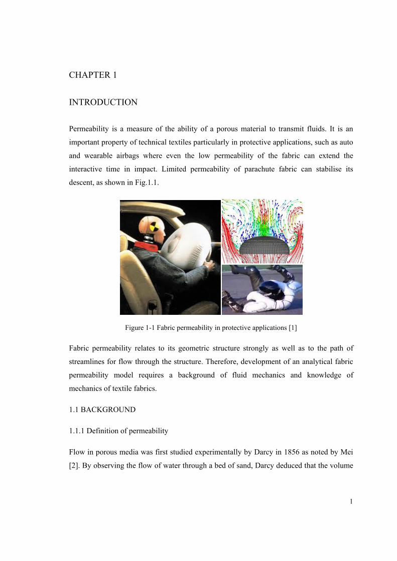
Permeability is a measure of the ability of a porous material to transmit fluids. It is an

important property of technical textiles particularly in protective applications, such as auto

and wearable airbags where even the low permeability of the fabric can extend the

interactive time in impact. Limited permeability of parachute fabric can stabilise its

descent, as shown in Fig.1.1.

Figure 1-1 Fabric permeability in protective applications [1]

Fabric permeability relates to its geometric structure strongly as well as to the path of

streamlines for flow through the structure. Therefore, development of an analytical fabric

permeability model requires a background of fluid mechanics and knowledge of

mechanics of textile fabrics.

1.1 BACKGROUND

1.1.1 Definition of permeability

Flow in porous media was first studied experimentally by Darcy in 1856 as noted by Mei

[2]. By observing the flow of water through a bed of sand, Darcy deduced that the volume

2

of water running through the sand is proportional to the pressure drop. The resulting

equation is the well known Darcy’s law: = ∆ (1-1)

Where is the total volumetric discharge in unit time, is the cross sectional area of the

porous medium, ∆ / is the pressure gradient, is the fluid viscosity and is the

permeability of the porous medium, which has a dimension with m2 after deduction.

Permeability arose from Darcy’s law where all the detailed microscopic interactions

between the fluid and the porous medium were lumped into the permeability value. As

such, it is a property of the porous medium. Its value depends on the geometry and the

structure of the flow channels in the porous medium. The permeability as defined in

Darcy’s law pertains to the steady flow of fluid in a saturated porous medium. Air

permeability tests within low constant Reynolds number ( , Appendix II) obey the law as

the air is absolutely saturated in the porous medium.

In the general case, permeability is a tensor and its components in three-dimensional space

are written as:

= (1-2)

For a woven fabric, the permeability tensor is orthotropic where = , =, = , and there exists a principal coordinate system with a principle

permeability tensor:

= 0 00 00 0 (1-3)

Where and can be regarded as the in-plane permeabilities while is the through-

thickness permeability. For a textile, fluid always tries to find the easiest flow path,

therefore, the gaps between yarns are the main flow channels and hence dominate the

3

permeability. Fluid flowing in three dimensions experience different resistance due to the

anisotropic textile structure, and generally the values of , and are different.

At a micro level for a yarn inside a textile, it has two permeabilities: along the fibre

permeability ( ∥) and perpendicular to the fibre permeability ( ). As yarns in a woven

fabric are undulating, the overall fabric permeability should involve the ∥ and values

along with the yarn crimp angle.

In this thesis, through-thickness permeability of woven fabric is tested experimentally

using a static permeability tester and a dynamic permeability tester, which are introduced

in Chapter 3 and 4 in detail. The static permeability tester provides a low and constant

pressure drop between fabric sides and the corresponding flow velocity is recorded as an

average value. The static permeability is calculated by substituting the pressure drop and

the velocity into Eq.1.1 with measured fabric thickness. The dynamic permeability tester

uses a constant volume tank which gives a clamped fabric a high initial pressure drop,

which falls as air flows through the fabric. The dynamic permeability is obtained by the

transient pressure drop and air velocity. The experimental process to obtain the fabric

through-thickness permeability can also be simulated by computational fluid dynamics

(CFD), which gives a flow velocity based on a set pressure drop. The simulated

permeabilities are obtained using the same theories as in the experimental approach.

1.1.2 Textile fabrics

A textile is a flexible material consisting of a network of bundles, natural or artificial

fibres often referred to as threads or yarns. Yarn might be monofilament, a bundle of

untwisted long filaments or produced by processes such as spinning raw short fibres of

cotton, flax, wool, silk, or other material to produce long strands. Textiles are formed by

weaving, knitting, crocheting, knotting or pressing fibres together. Most fabrics can bend

and fold easily. Textile fabrics can be loose or tight depending on the amount of gaps in

their structure. Therefore, textile fabrics are thin, flexible, porous sheet materials. They are

used extensively in our daily lives and in mainly industries, for example medical textiles

(e.g., implants), geo-textiles (reinforcement of embankments) and protective clothing (e.g.,

heat and radiation protection for fire fighter clothing, airbags for road vehicles, etc.).

4

(a), Geometry of textiles

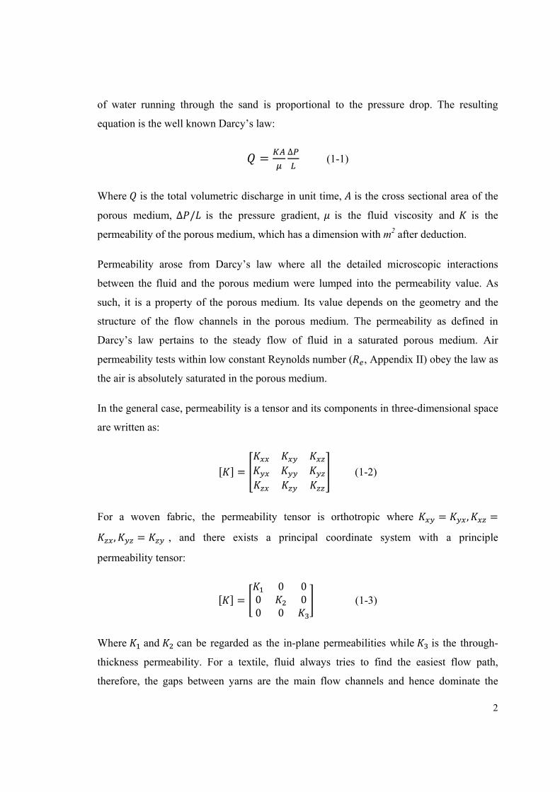
In this thesis, woven fabrics are studied. One-layer woven fabrics consist of generally two

orthogonal series of yarns, referred to as warp and weft yarns, interlaced to form a self-

supporting textile architecture. 3D woven fabric usually contains warp and weft yarns as

well as through-thickness yarns to bind them. A number of fabric structures are shown in

Fig.1.2:

2D Plain weave 2D 2/1 Twill weave

2D 5/3 Satin weave 3D Orthogonal weave

Figure 1-2 Images of woven fabric architectures (generated by TexGen [3])

The simplest of interlacing patterns is the plain weave (such as the 2D plain weave in

Fig.1.2). It is the most basic type of textile weave with the warp and weft aligned so they

form a simple criss-cross pattern. Each weft thread crosses the warp threads by going over

one, then under the next, and so on. More complex interlacing patterns for one-layer

woven fabric can be categorised as twill, satin, crowfoot, rib, basket, herringbone, crepe,

5

etc. A twill weave (such as the 2/1 twill in Fig.1.2) is the second most basic weave that can

be made on a simple loom. In a twill weave, each weft yarn floats across the warp yarns in

a progression of interlacings to the right or left, forming a distinct diagonal line. The

diagonal line is also known as a ‘wale’. A float is the portion of a yarn that crosses over

two or more yarns from the opposite direction. Twill weave is often designated as a

fraction, such as 2/1, in which the numerator indicates the number of harnesses that are

raised when a weft yarn is inserted. A satin weave (such as the 5/3 satin weave in Fig.1.2)

is characterized by four or more weft yarns floating over a warp yarn or vice versa, four or

more warp yarns floating over a single weft yarn. The structure of a satin weave is not

stable as the long floating yarns travel over other perpendicular yarns.

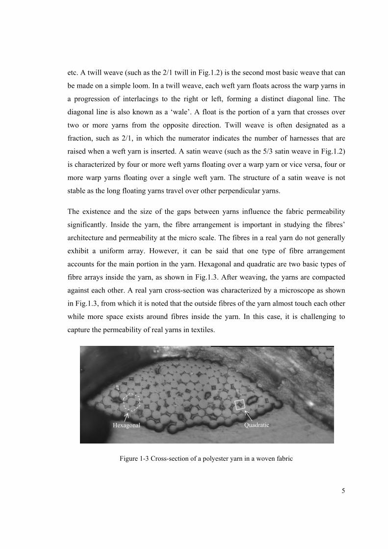
The existence and the size of the gaps between yarns influence the fabric permeability

significantly. Inside the yarn, the fibre arrangement is important in studying the fibres’

architecture and permeability at the micro scale. The fibres in a real yarn do not generally

exhibit a uniform array. However, it can be said that one type of fibre arrangement

accounts for the main portion in the yarn. Hexagonal and quadratic are two basic types of

fibre arrays inside the yarn, as shown in Fig.1.3. After weaving, the yarns are compacted

against each other. A real yarn cross-section was characterized by a microscope as shown

in Fig.1.3, from which it is noted that the outside fibres of the yarn almost touch each other

while more space exists around fibres inside the yarn. In this case, it is challenging to

capture the permeability of real yarns in textiles.

Figure 1-3 Cross-section of a polyester yarn in a woven fabric

Hexagonal Quadratic

6

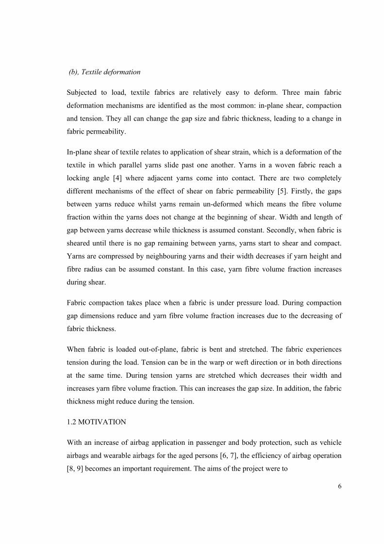
(b), Textile deformation

Subjected to load, textile fabrics are relatively easy to deform. Three main fabric

deformation mechanisms are identified as the most common: in-plane shear, compaction

and tension. They all can change the gap size and fabric thickness, leading to a change in

fabric permeability.

In-plane shear of textile relates to application of shear strain, which is a deformation of the

textile in which parallel yarns slide past one another. Yarns in a woven fabric reach a

locking angle [4] where adjacent yarns come into contact. There are two completely

different mechanisms of the effect of shear on fabric permeability [5]. Firstly, the gaps

between yarns reduce whilst yarns remain un-deformed which means the fibre volume

fraction within the yarns does not change at the beginning of shear. Width and length of

gap between yarns decrease while thickness is assumed constant. Secondly, when fabric is

sheared until there is no gap remaining between yarns, yarns start to shear and compact.

Yarns are compressed by neighbouring yarns and their width decreases if yarn height and

fibre radius can be assumed constant. In this case, yarn fibre volume fraction increases

during shear.

Fabric compaction takes place when a fabric is under pressure load. During compaction

gap dimensions reduce and yarn fibre volume fraction increases due to the decreasing of

fabric thickness.

When fabric is loaded out-of-plane, fabric is bent and stretched. The fabric experiences

tension during the load. Tension can be in the warp or weft direction or in both directions

at the same time. During tension yarns are stretched which decreases their width and

increases yarn fibre volume fraction. This can increases the gap size. In addition, the fabric

thickness might reduce during the tension.

1.2 MOTIVATION

With an increase of airbag application in passenger and body protection, such as vehicle

airbags and wearable airbags for the aged persons [6, 7], the efficiency of airbag operation

[8, 9] becomes an important requirement. The aims of the project were to

7

• Understand the fundamental flow behaviour in textile materials;

• Analyze the structures of airbag fabrics and common clothing fabrics; test the air

permeability of those fabrics when air transfers through them; develop an

analytical model relating the air permeability to textile structure;

• Simulate fabric behaviour in real airbag inflation; determine the effect of pressure

drop on the fabric permeability;

• Develop an analytical model to relate fabric deformation and corresponding

permeability to pressure load; verify this by simulation and experiment;

The original work focused on airbag fabric. Therefore through-thickness permeability is

the main permeability discussed in this thesis.

In Saldaeva’s thesis [10], the air permeabilities of several woven fabrics were measured

under low pressure drops using an air permeability tester FX3300. The author plotted the

relationship of pressure drop and fluid velocity for each fabric and found a linear

relationship. With the application of Eq.1.1, the air permeability of each fabric was

calculated experimentally. However, the gaps between the yarns in each fabric are

different geometrically. One fixed structure of fabric has a constant permeability.

Therefore what is the relationship of the fabric permeability with its structure, or the

geometry of the flow channel inside the fabric? From observations of fabric structures by

microscopy, it is noted that the yarns in tight fabrics are overlapping while the loose

fabrics have clear gaps between yarns. In addition, the gaps between yarns in loose fabrics

are not analogous to straight pipes. They are actually more like the gradually converging-

diverging tubes, depending on the geometry of the yarn cross-sections. If the geometries of

the gaps or the fabrics are not deformable, there will be an obvious nonlinear relationship

of pressure drop and fluid velocity when the fabric is under a series of high pressure drops.

Therefore, what is the permeability under high pressure if the fabric structure is known?

As airbag fabrics undergo very high pressure inflation, the fabrics are deformed when

subjected to such high distributed loads, leading to new structures and geometries of flow

channels. For instance, for a clamped loose fabric under a uniform distributed load, its

thickness gets smaller while its gap between yarns can become larger due to its in-plane

8

tension. Therefore, how do we predict the change of fabric geometry under high pressure

load? What is the relationship between pressure and permeability?

1.3 OVERVIEW OF THESIS

This thesis presents studies to predict through-thickness permeability of woven fabric. A

unified analytical model has been systematically developed to predict the fabric static

permeability. Dynamic permeability was tested experimentally. Fabric deformation and

corresponding permeability were also modelled analytically. The objective was to

understand the relationship between fluid flow and fabric structure. A wide range of

woven fabrics were considered including tight fabrics and loose fabrics. Analytical

permeability predictions for these fabrics were all compared with experimental data. In

addition, the analytical predictions were compared with CFD (computational fluid

dynamics) simulations. The structure of the thesis is outlined below.

Chapter 2 firstly provides a literature review on analytical, numerical modelling and

experimental investigation of static permeability of porous media. It presents the

development of the models and the limitation of each model. Secondly, a review on

dynamic permeability is presented, including experimental and computational work. This

is followed by a review of fabric deformation under pressure load and the fundamental

theory for fabric deformation. The fourth section reviews research on the nonlinear

relationship of pressure and fluid velocity.

Chapter 3 focuses on the development of an analytical model for through-thickness static

permeability of woven fabric. For flow through gaps between yarns in a woven fabric, an

analytical model is developed based on viscous and incompressible Hagen-Poiseuille flow.

The flow is modelled through a unit cell of fabric with a smooth fluid channel at the centre

with slowly varying cross-section. The channel geometry is determined by yarn spacing,

yarn cross-section and fabric thickness. The shape of channel is approximately by a

parabolic function. Volumetric flow rate is formulated as a function of pressure drop and

flow channel geometry for woven fabric. The gap permeability is calculated thereafter

according to Darcy’s law. The analytical model is verified by CFD simulations and

experimental determination. This chapter then reviews analytical models for flow through

9

yarns in a woven fabric. A unified analytical model integrates the permeability equations

for gaps between yarns and yarns in woven fabrics in terms of fabric porosity for through-

thickness permeability of any woven fabric. Through-thickness static permeability of 3D

woven fabric is predicted based on one-layer of woven fabric structure. All predictions are

verified by numerical simulation and experimental tests.

Chapter 4 presents a definition of dynamic permeability and utilizes a reliable approach to

measure and characterize dynamic permeability for woven fabrics. The experimental

principle is based on the ideal gas law and the non-linear Forchheimer equation. Tight and

loose fabrics are both tested for dynamic permeability, which is compared with their static

permeability. Effects of increased number of fabric layers and initial pressure level are

investigated.

Chapter 5 contains two sections. An analytical model is developed to predict fabric

deformation under high pressure load. The model is based on an energy approach

including strain energy, bending energy and work done on the fabric. A vacuum-based

device is designed to verify the analytical model experimentally. The second section

analyzes the effects of fabric deformation on its through-thickness permeability based on a

number of assumptions. The fabric permeability prediction in this case is also compared

with experimental values of the dynamic permeability.

Chapter 6 extends Darcy flow to non-Darcy flow, which analyzes the quantification of

hydraulic resistance to laminar flow at high Reynolds number. The model uses a gradual

converging-diverging flow channel. A nonlinear relationship between pressure and flow

velocity is given by adding a non-Darcy term, which is based on continuity theory and the

Bernoulli equation. The main features of the model are that the Darcy flow is a function of

the fluid property and channel geometry while the non-Darcy flow depends on the channel

geometry completely. The non-Darcy model for predicting the nonlinear relationship is

verified by CFD simulations and experimental data. This nonlinear relationship is due to

the gap geometry, which is compared with the fabric deformation effects in the last section.

Chapter 7 gives an overall summary and conclusions of the present work and

recommendations for future work.

10

CHAPTER 2

LITERATURE REVIEW

2.1 INTRODUCTION

For a porous material, static permeability defines the ability to transmit permeating fluid at

a constant pressure drop, while dynamic permeability concerns mass transport under

transient pressure conditions. Static permeability, normally measured under low pressure

drop (≤500Pa), is one of the primary properties for technical textiles used in fluid related

applications such as textile composites processing, paper making, air and water filtration.

Dynamic permeability is another important property for many technical textiles such as

automotive airbags, wearable (landing) airbags and parachute fabrics. These fabrics are

usually subjected to high initial pressure, for example, a car airbag fabric is subjected to

200 KPa higher than atmospheric pressure. This may result in deformation of the fabric

structure, leading to a change in the permeability.

There are two kinds of woven fabric, loose fabric (clear gap between yarns) and tight

fabric (overlapping yarns in fabric). For a loose fabric, the regular interwoven structure of

woven fabric gives rise to arrays of fluid channels. These channels are in theory identical

and repetitive. The geometry of each individual channel depends mainly on weave density,

yarn shape and weave style. Fabric permeability is governed by these geometric

parameters. For a tight fabric, fluid has to transfer through the yarns. Fibre radius,

arrangement and volume fraction become the main geometric factors determining the yarn

permeability. In addition, undulating yarn shape in woven fabric also affects the fabric

permeability to some extent. A predictive model of permeability as a function of fabric

structure is a desirable tool for optimum materials design [11].

For laminar flow, there are linear and nonlinear relationships of pressure drop and fluid

velocity. The former relationship is defined as Darcy flow while the latter is referred to as

non-Darcy flow. When pressure drop increases in a converging-diverging flow channel,

the appearance of non-Darcy flow is due to the flow convective acceleration. In addition,

11

the fabric deformation under loading can change the fabric geometric dimensions, leading

to a change in permeability. An analytical model to predict permeability as a function of

fabric geometry and loading is required for understanding of the underlying mechanisms.

2.2 DARCY FLOW IN POROUS MEDIA

As introduced in Section 1.1.1, Eq.1.1 is an empirical equation describing the relationship

of pressure gradient and volumetric flow rate. Early developments of Darcy’s law were

spurred on by studies in hydrology and soil mechanics. The applications normally

considered of granular beds (sand and rocks) or porous solids, which are assumed to be

isotropic and homogeneous. Subsequently it was observed that directional variations of

permeability can occur. For a macroscopically homogeneous piece of rock, the

permeability is not the same across different cross-sectional faces [12]. In fibre composites

engineering, most fibre preforms are heterogeneous materials and exhibit anisotropic flow

behaviour. The theory of flow in anisotropic materials was developed particularly by

Farrandon in 1948 and Liwiniszyn in 1950 [13], through which the full tensorial form of

Darcy’s law (Eq.1.26) for anisotropic media was derived:

= − ∇ (2-1)

Where is the superficial velocity, which is obtained in a macroscopic scale; is the fluid

viscosity; ∇ is the pressure gradient and is the permeability tensor of the porous

medium.

Research on the air permeability of textile materials began at the end of the 19th century

when experimental methods for estimating the hygienic properties of materials for clothing

began to be used [14]. The first studies of air permeability for fabrics conducted by Rubber

[15] were based on Darcy’s law. Burschke and Advani[16] reported excellent agreement

using experiment and numerical simulation for Newtonian fluid through a fibre network

compared with Darcy’s law. However, Darcy’s law does not relate the structural

parameters of porous materials to the value of permeability.

12

Kozeny and Carman [17] found a similar relation between pressure drop and flow velocity

as in Darcy’s law separately, suggesting that the permeability is independently determined

by material variables i.e. porosity (∅) and specific surface area ( ):

= ∅( ∅) (2-2)

Where is the Kozeny coefficient, ∅ is defined as the portion of total space inside a

porous medium. This classical permeability-porosity equation was originally developed

for granular beds consisting of ellipsoids. Further modification of the equation made it

applicable in various fields subsequently [18, 19], such as fouled fibrous filters and

adsorbents, and other composite porous media. However, one weakness of the Kozeny-

Carman equation was pointed out by Gutowski [20] when applied to composites

manufacturing in that the model parameters are only coupled to the geometry through the

variables on radius of fibre and that the detailed geometry dependence is lumped together

into the model parameter which has to be determined experimentally. Published results

also indicated that the parameter may vary with the fibre volume fraction for a given

fabric [21].

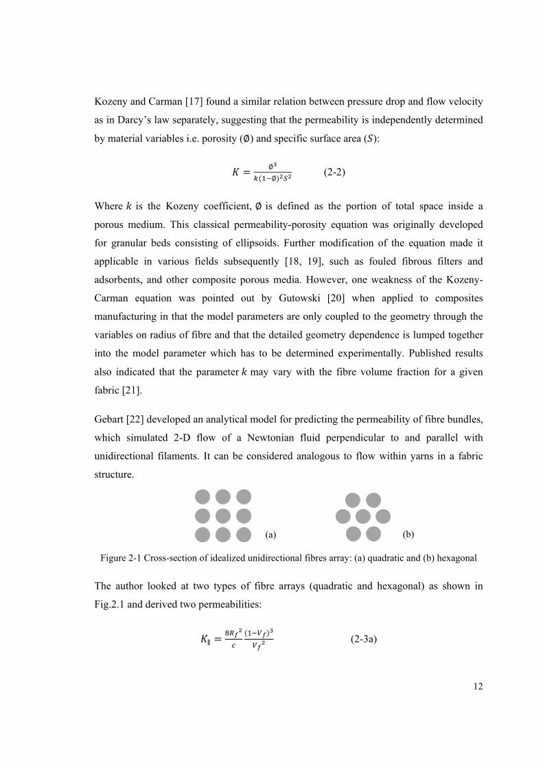
Gebart [22] developed an analytical model for predicting the permeability of fibre bundles,

which simulated 2-D flow of a Newtonian fluid perpendicular to and parallel with

unidirectional filaments. It can be considered analogous to flow within yarns in a fabric

structure.

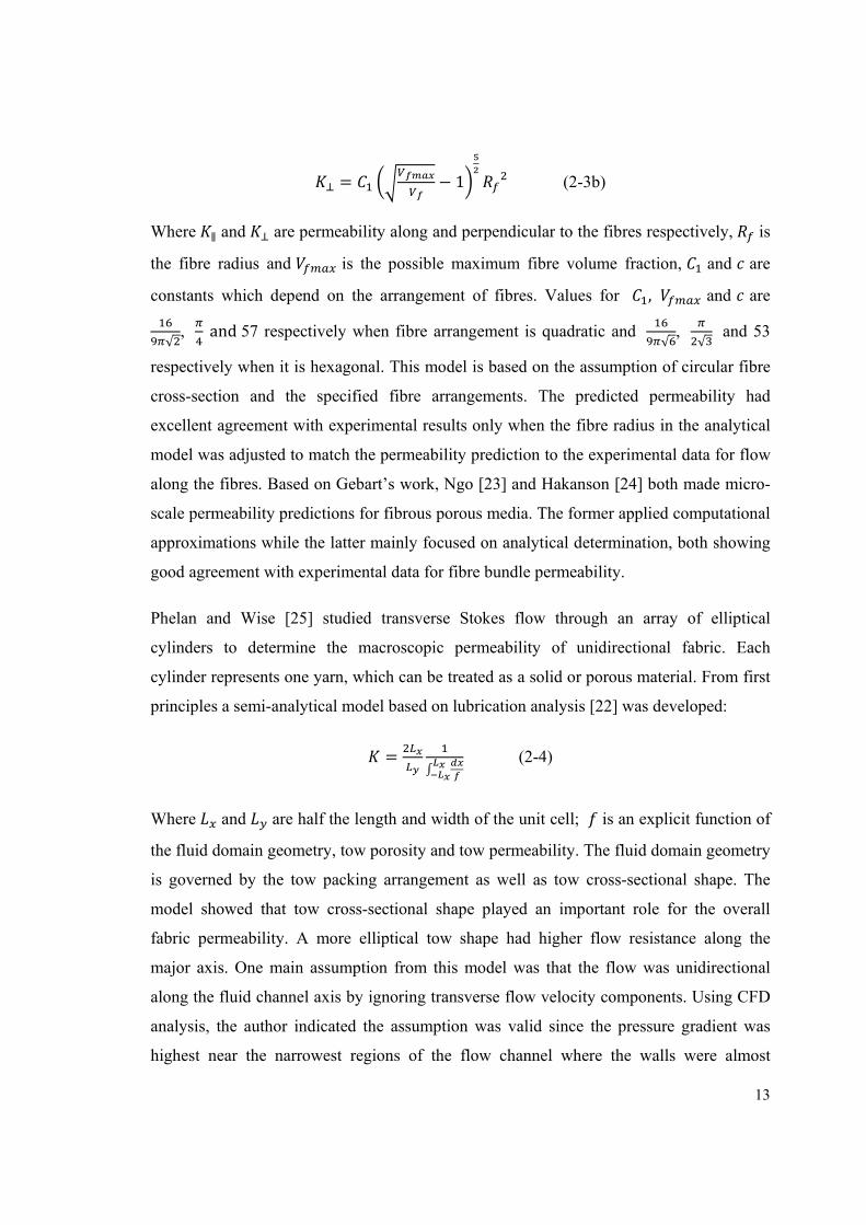
Figure 2-1 Cross-section of idealized unidirectional fibres array: (a) quadratic and (b) hexagonal

The author looked at two types of fibre arrays (quadratic and hexagonal) as shown in

Fig.2.1 and derived two permeabilities:

∥ = ( ) (2-3a)

(a) (b)

13

= − 1 (2-3b)

Where ∥ and are permeability along and perpendicular to the fibres respectively, is

the fibre radius and is the possible maximum fibre volume fraction, and are

constants which depend on the arrangement of fibres. Values for , and are

√ , and 57 respectively when fibre arrangement is quadratic and √ , √ and 53

respectively when it is hexagonal. This model is based on the assumption of circular fibre

cross-section and the specified fibre arrangements. The predicted permeability had

excellent agreement with experimental results only when the fibre radius in the analytical

model was adjusted to match the permeability prediction to the experimental data for flow

along the fibres. Based on Gebart’s work, Ngo [23] and Hakanson [24] both made micro-

scale permeability predictions for fibrous porous media. The former applied computational

approximations while the latter mainly focused on analytical determination, both showing

good agreement with experimental data for fibre bundle permeability.

Phelan and Wise [25] studied transverse Stokes flow through an array of elliptical

cylinders to determine the macroscopic permeability of unidirectional fabric. Each

cylinder represents one yarn, which can be treated as a solid or porous material. From first

principles a semi-analytical model based on lubrication analysis [22] was developed:

= (2-4)

Where and are half the length and width of the unit cell; is an explicit function of

the fluid domain geometry, tow porosity and tow permeability. The fluid domain geometry

is governed by the tow packing arrangement as well as tow cross-sectional shape. The

model showed that tow cross-sectional shape played an important role for the overall

fabric permeability. A more elliptical tow shape had higher flow resistance along the

major axis. One main assumption from this model was that the flow was unidirectional

along the fluid channel axis by ignoring transverse flow velocity components. Using CFD

analysis, the author indicated the assumption was valid since the pressure gradient was

highest near the narrowest regions of the flow channel where the walls were almost

14

parallel. The model improves the permeability prediction by considering specific

geometries [26]. However it is not directly applicable to woven fabric where the flow

domain geometry is more complex.

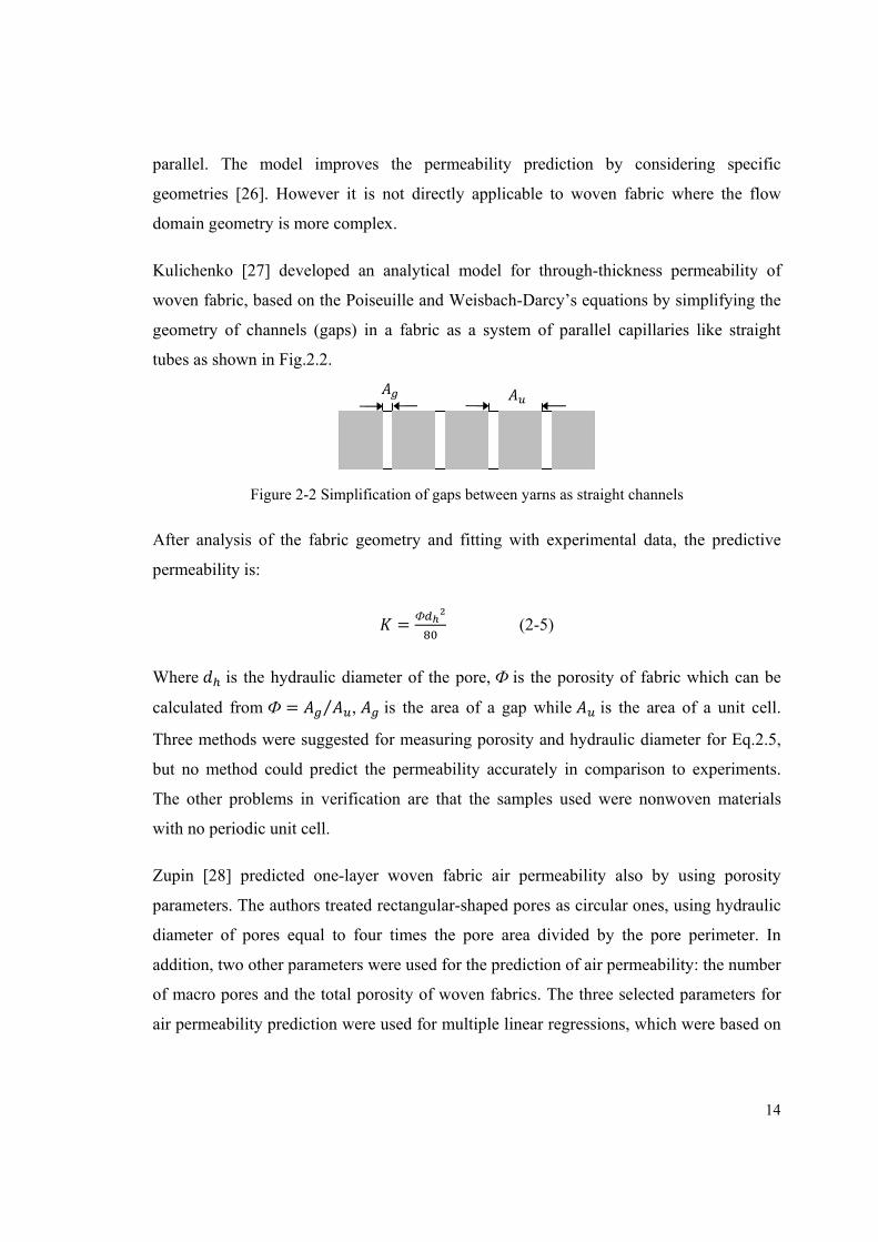
Kulichenko [27] developed an analytical model for through-thickness permeability of

woven fabric, based on the Poiseuille and Weisbach-Darcy’s equations by simplifying the

geometry of channels (gaps) in a fabric as a system of parallel capillaries like straight

tubes as shown in Fig.2.2.

Figure 2-2 Simplification of gaps between yarns as straight channels

After analysis of the fabric geometry and fitting with experimental data, the predictive

permeability is:

= Ф (2-5)

Where is the hydraulic diameter of the pore, Ф is the porosity of fabric which can be

calculated from Ф = ⁄ , is the area of a gap while is the area of a unit cell.

Three methods were suggested for measuring porosity and hydraulic diameter for Eq.2.5,

but no method could predict the permeability accurately in comparison to experiments.

The other problems in verification are that the samples used were nonwoven materials

with no periodic unit cell.

Zupin [28] predicted one-layer woven fabric air permeability also by using porosity

parameters. The authors treated rectangular-shaped pores as circular ones, using hydraulic

diameter of pores equal to four times the pore area divided by the pore perimeter. In

addition, two other parameters were used for the prediction of air permeability: the number

of macro pores and the total porosity of woven fabrics. The three selected parameters for

air permeability prediction were used for multiple linear regressions, which were based on

15

experimental measurements. The high coefficient of correlation (R2) value of 0.94

indicated the model explained variability in the air permeability to a large extent.

To summarize up to this point, Kozeny developed an analytical equation containing a

fitting coefficient for any porous medium; Gebart derived a set of equations describing

flow along and perpendicular to unidirectional fibre arrays, assuming two idealized types

of packing; Phelan gave a semi-analytical equation considering the tow shape in the fabric;

Kulichenko’s model assumes the gaps inside the fabric are a system of parallel capillaries,

which cannot be used to model textile fabrics accurately as this does not consider the

curvature of yarn cross-sections. Zupin treated the rectangular-shaped gaps as circular

ones in woven fabric by using hydraulic diameter, which is a useful reference for the

development of an analytical model in this thesis.

Other analytical models for permeability of fibre arrays have also been developed to relate

fibre volume fraction ( ) and geometric or empirical constants such as the maximum

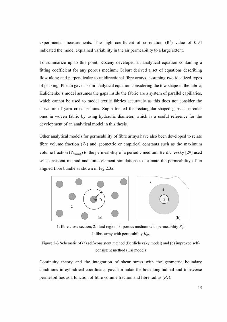
volume fraction ( ) to the permeability of a periodic medium. Berdichevsky [29] used

self-consistent method and finite element simulations to estimate the permeability of an

aligned fibre bundle as shown in Fig.2.3a.

1: fibre cross-section; 2: fluid region; 3: porous medium with permeability ;

4: fibre array with permeability

Figure 2-3 Schematic of (a) self-consistent method (Berdichevsky model) and (b) improved self-

consistent method (Cai model)

Continuity theory and the integration of shear stress with the geometric boundary

conditions in cylindrical coordinates gave formulae for both longitudinal and transverse

permeabilities as a function of fibre volume fraction and fibre radius ( ):

(b) (a)

1

2

2

4

3

16

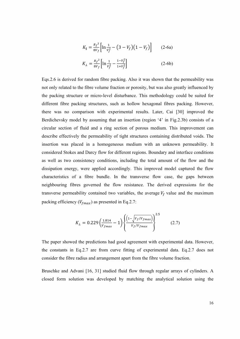
∥ = ln − 3 − 1 − (2-6a)

= ln − (2-6b)

Eqs.2.6 is derived for random fibre packing. Also it was shown that the permeability was

not only related to the fibre volume fraction or porosity, but was also greatly influenced by

the packing structure or micro-level disturbance. This methodology could be suited for

different fibre packing structures, such as hollow hexagonal fibres packing. However,

there was no comparison with experimental results. Later, Cai [30] improved the

Berdichevsky model by assuming that an insertion (region ‘4’ in Fig.2.3b) consists of a

circular section of fluid and a ring section of porous medium. This improvement can

describe effectively the permeability of tight structures containing distributed voids. The

insertion was placed in a homogeneous medium with an unknown permeability. It

considered Stokes and Darcy flow for different regions. Boundary and interface conditions

as well as two consistency conditions, including the total amount of the flow and the

dissipation energy, were applied accordingly. This improved model captured the flow

characteristics of a fibre bundle. In the transverse flow case, the gaps between

neighbouring fibres governed the flow resistance. The derived expressions for the

transverse permeability contained two variables, the average value and the maximum

packing efficiency ( ) as presented in Eq.2.7:

= 0.229 . − 1 ⁄⁄.

(2.7)

The paper showed the predictions had good agreement with experimental data. However,

the constants in Eq.2.7 are from curve fitting of experimental data. Eq.2.7 does not

consider the fibre radius and arrangement apart from the fibre volume fraction.

Bruschke and Advani [16, 31] studied fluid flow through regular arrays of cylinders. A

closed form solution was developed by matching the analytical solution using the

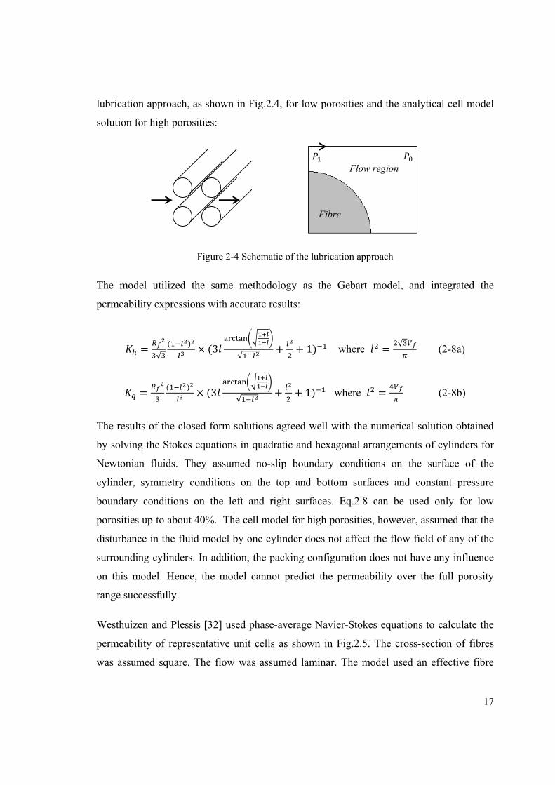
17

lubrication approach, as shown in Fig.2.4, for low porosities and the analytical cell model

solution for high porosities:

Figure 2-4 Schematic of the lubrication approach

The model utilized the same methodology as the Gebart model, and integrated the

permeability expressions with accurate results:

= √ ( ) × (3 √ + + 1) where = √ (2-8a)

= ( ) × (3 √ + + 1) where = (2-8b)

The results of the closed form solutions agreed well with the numerical solution obtained

by solving the Stokes equations in quadratic and hexagonal arrangements of cylinders for

Newtonian fluids. They assumed no-slip boundary conditions on the surface of the

cylinder, symmetry conditions on the top and bottom surfaces and constant pressure

boundary conditions on the left and right surfaces. Eq.2.8 can be used only for low

porosities up to about 40%. The cell model for high porosities, however, assumed that the

disturbance in the fluid model by one cylinder does not affect the flow field of any of the

surrounding cylinders. In addition, the packing configuration does not have any influence

on this model. Hence, the model cannot predict the permeability over the full porosity

range successfully.

Westhuizen and Plessis [32] used phase-average Navier-Stokes equations to calculate the

permeability of representative unit cells as shown in Fig.2.5. The cross-section of fibres

was assumed square. The flow was assumed laminar. The model used an effective fibre

Fibre

Flow region

18

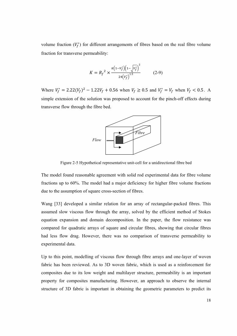
volume fraction ( ∗) for different arrangements of fibres based on the real fibre volume

fraction for transverse permeability:

= × ∗ ∗∗ . (2-9)

Where ∗ = 2.22( ) − 1.22 + 0.56 when ≥ 0.5 and ∗ = when < 0.5 . A

simple extension of the solution was proposed to account for the pinch-off effects during

transverse flow through the fibre bed.

Figure 2-5 Hypothetical representative unit-cell for a unidirectional fibre bed

The model found reasonable agreement with solid rod experimental data for fibre volume

fractions up to 60%. The model had a major deficiency for higher fibre volume fractions

due to the assumption of square cross-section of fibres.

Wang [33] developed a similar relation for an array of rectangular-packed fibres. This

assumed slow viscous flow through the array, solved by the efficient method of Stokes

equation expansion and domain decomposition. In the paper, the flow resistance was

compared for quadratic arrays of square and circular fibres, showing that circular fibres

had less flow drag. However, there was no comparison of transverse permeability to

experimental data.

Up to this point, modelling of viscous flow through fibre arrays and one-layer of woven

fabric has been reviewed. As to 3D woven fabric, which is used as a reinforcement for

composites due to its low weight and multilayer structure, permeability is an important

property for composites manufacturing. However, an approach to observe the internal

structure of 3D fabric is important in obtaining the geometric parameters to predict its

Fibre

Flow

19

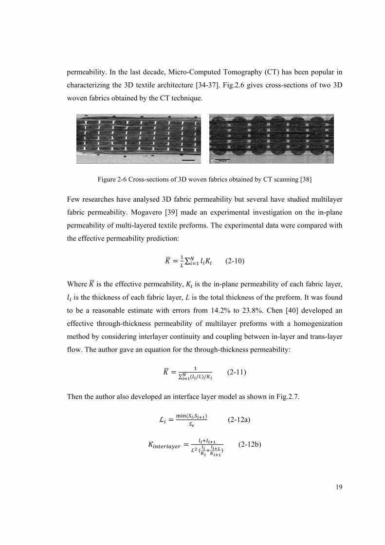
permeability. In the last decade, Micro-Computed Tomography (CT) has been popular in

characterizing the 3D textile architecture [34-37]. Fig.2.6 gives cross-sections of two 3D

woven fabrics obtained by the CT technique.

Figure 2-6 Cross-sections of 3D woven fabrics obtained by CT scanning [38]

Few researches have analysed 3D fabric permeability but several have studied multilayer

fabric permeability. Mogavero [39] made an experimental investigation on the in-plane

permeability of multi-layered textile preforms. The experimental data were compared with

the effective permeability prediction:

= ∑ (2-10)

Where is the effective permeability, is the in-plane permeability of each fabric layer,

is the thickness of each fabric layer, L is the total thickness of the preform. It was found

to be a reasonable estimate with errors from 14.2% to 23.8%. Chen [40] developed an

effective through-thickness permeability of multilayer preforms with a homogenization

method by considering interlayer continuity and coupling between in-layer and trans-layer

flow. The author gave an equation for the through-thickness permeability:

= ∑ ( / )/ (2-11)

Then the author also developed an interface layer model as shown in Fig.2.7.

ℒ = ( , ) (2-12a)

= ℒ ( ) (2-12b)

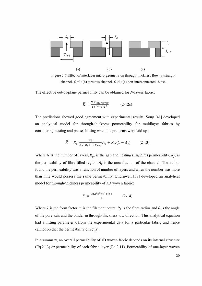
20

(a) (b) (c)

Figure 2-7 Effect of interlayer micro-geometry on through-thickness flow (a) straight

channel, ℒ =1; (b) tortuous channel, ℒ >1; (c) non-interconnected, ℒ =∞.

The effective out-of-plane permeability can be obtained for N-layers fabric:

= ( )ℒ (2-12c)

The predictions showed good agreement with experimental results. Song [41] developed

an analytical model for through-thickness permeability for multilayer fabrics by

considering nesting and phase shifting when the preforms were laid up:

= ⋯ + (1 − ) (2-13)

Where is the number of layers, is the gap and nesting (Fig.2.7c) permeability, is

the permeability of fibre-filled region, is the area fraction of the channel. The author

found the permeability was a function of number of layers and when the number was more

than nine would possess the same permeability. Endruweit [38] developed an analytical

model for through-thickness permeability of 3D woven fabric:

= (2-14)

Where is the form factor, is the filament count, is the fibre radius and is the angle

of the pore axis and the binder in through-thickness tow direction. This analytical equation

had a fitting parameter from the experimental data for a particular fabric and hence

cannot predict the permeability directly.

In a summary, an overall permeability of 3D woven fabric depends on its internal structure

(Eq.2.13) or permeability of each fabric layer (Eq.2.11). Permeability of one-layer woven

21

fabric is determined by the fabric geometric features, such as gap shape and fabric

thickness. In a fibre bundle, tow permeability is a function of fibre radius and fibre volume

fraction. However, the reviewed models did not consider either the shape of streamlines in

the fabric gaps nor the flow transverse to the undulating yarns in a fabric. An analytical

model is required for predicting the static permeability of woven fabrics based on

geometric features without any fitting factors.

2.3 NON-DARCY FLOW IN POROUS MEDIA

When a creeping flow develops in a porous medium under a low pressure drop, it reveals a

linear relationship between the pressure drop and the flow velocity. While the pressure

drop increases, leading to a higher value but still laminar, a non-linear relationship

appears. This means Darcy’s law cannot be used for accurate flow analysis in this case.

This was first proposed by Forchheimer in 1901 as noted by Skjetne [42] to give a high-

velocity correction to Darcy’s law with a power of velocity:

− = + (2-15)

Where is called the Darcy coefficient, and m is close to 2. Forchheimer also proposed

that the pressure loss could be expressed by a third order polynomial in velocity:

− = + + (2-16)

Based on a dimensional analysis by Green and Duwez [43], Cornell and Katz [44], the

coefficients in Eq.2.15 with m = 2, can be separated as fluid and porous media parameters,

resulting in what is today called the Forchheimer equation:

− = V + βV (2-17)

Where equals μ , β is a porous media parameter called the non-Darcy flow coefficient.

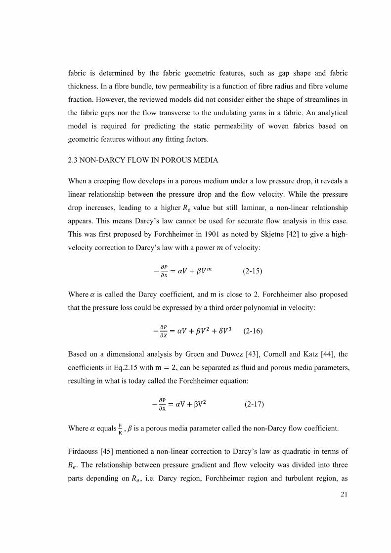
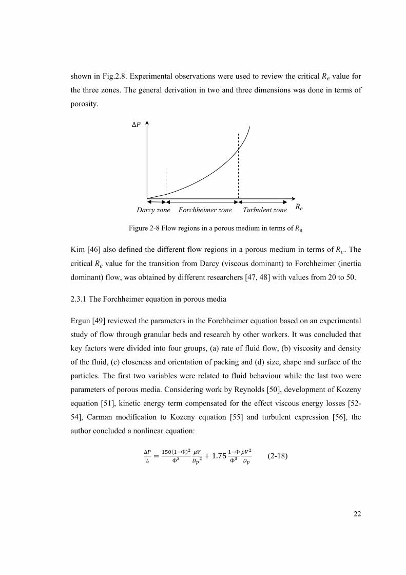
Firdaouss [45] mentioned a non-linear correction to Darcy’s law as quadratic in terms of

. The relationship between pressure gradient and flow velocity was divided into three

parts depending on , i.e. Darcy region, Forchheimer region and turbulent region, as

22

shown in Fig.2.8. Experimental observations were used to review the critical value for

the three zones. The general derivation in two and three dimensions was done in terms of

porosity.

Figure 2-8 Flow regions in a porous medium in terms of

Kim [46] also defined the different flow regions in a porous medium in terms of . The

critical value for the transition from Darcy (viscous dominant) to Forchheimer (inertia

dominant) flow, was obtained by different researchers [47, 48] with values from 20 to 50.

2.3.1 The Forchheimer equation in porous media

Ergun [49] reviewed the parameters in the Forchheimer equation based on an experimental

study of flow through granular beds and research by other workers. It was concluded that

key factors were divided into four groups, (a) rate of fluid flow, (b) viscosity and density

of the fluid, (c) closeness and orientation of packing and (d) size, shape and surface of the

particles. The first two variables were related to fluid behaviour while the last two were

parameters of porous media. Considering work by Reynolds [50], development of Kozeny

equation [51], kinetic energy term compensated for the effect viscous energy losses [52-

54], Carman modification to Kozeny equation [55] and turbulent expression [56], the

author concluded a nonlinear equation:

∆ = ( Ф)Ф

+ 1.75 Ф

Ф (2-18)

Darcy zone Forchheimer zone Turbulent zone

∆

23

Where ∆

is the pressure gradient, is the solid particle diameter, relating to the specific

surface area , = . Eq.2.18 is suited for nonlinear flow in a granular bed.

Brasquet [57] used classical models and neural networks, and validated this with

experimental data, for pressure drop through textile fabrics. The author reviewed briefly

the development of nonlinear relationship of pressure drop and flow velocity based on the

Eq.2.17. His analysis was based on a modified Ergun equation [49]. In order to compute

two physical parameters, the tortuosity factor ℒ and the dynamic specific surface area ,

Kyan [58], Dullien [59] developed the equations:

ℒ = ( Ф( . ) ) . (2-19a)

= ( ( . )( ) Ф( Ф) ) . (2-19b)

Based on the research of Renaud [60], another nonlinear equation was developed:

∆ = 2ℒ ( Ф)Ф

+ 0.0968ℒ Ф

Ф (2-20)

The application of Eq.2.20 is for particles of low thickness-to-side ratio (wood chips),

while its drawback is time consuming calculations to determine the parameters ( & in

Eq.2.19). Belkacemi and Broadbent [61] separated the Forchheimer equation into three

presume losses in the applications of stacking of fibres and woven yarns:

∆ = ∆ + ∆ + ∆ (2-21)

Where the first term is from viscous force, the second is from inertial force, the third is

based on the transformation from Kyan’s model [58]. Innocentini [62] considered the

influence of air compressibility on the permeability evaluation that gave a modification of

the Forchheimer equation:

= + (2-22)

24

Where is the fluid pressure at the entrance, is the pressure at the exit, is the

average value of and . Eq.2.22 can only be used when M is greater than 0.3 [63].

Theoretically, some researchers derived the Forchheimer equation from the Navier-Stokes

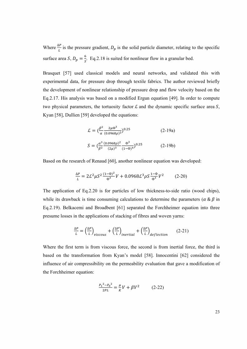
equation. Whitaker [64] used a volume averaging approach to derive Darcy’s law and the

Forchheimer correction for a homogeneous porous medium. The work began from the

Navier-Stokes equations and found the volume averaged momentum equation:

< >= − ∙ − − ∙< > (2-23)

Where < > is the average superficial velocity in the (fluid) phase, which is shown

in Fig.2.9, μ and ρ are the viscosity and density of the phase respectively, is the

acceleration due to gravity.

Figure 2-9 phase flow in a porous medium

The Darcy’s law permeability and the Forchheimer correction coefficient were

determined from closure problems, using a spatially periodic model of the porous medium.

However, the author did not give the analytical expressions of and as functions of the

geometric parameters of the porous medium.

Chen [65] derived the Forchheimer equation via the theory of homogenization. The

nonlinear correction to Darcy’s law was studied due to the inertial effects in Newtonian

flow in rigid porous media. A general formula for this correction term was derived directly

from the Navier-Stokes equations by homogenization:

− < > + < >= ( − ∇ ) (2-24)

25

Where is the Forchheimer tensor which is a function of velocity ( ). Unlike other

studies (Mei [66]; Wodie [67]) based on a similar approach which suggested that for the

nonlinear correction was cubic in velocity for isotropic media, this study showed the

nonlinear correction was quadratic. The paper also gave examples to illustrate the

quadratic correction, considering incompressible and compressible cases. The author

proved the validity of the Forchheimer equation in theory but did not compare the

analytical results with experimental data.

Burcharth [68] discussed porous flow in a coarse granular medium with special concern

given to the dependence of the flow resistance on the porosity. Steady state flow was

derived from the Navier-Stokes equations. Alternative derivations based on dimensional

analysis and a pipe analogy were discussed. For one dimensional steady flow, the author

obtained:

∆ = ′ Ф

Ф Ф+ ′ Ф

Ф(Ф) (2-25)

Where is the granular diameter, ′ depends on , the gradation and the grain shape. ′ depends on the same parameters plus the relative surface roughness of the grains. Eq.2.25

has the same style as Eq.2.18. It is also used for granular materials. The author discussed

the parameters ′and ′ in Forchheimer flow and turbulent flow states, which were both

expressed as functions of .

Skjetne [69] modelled high-velocity flow in porous media with a multiple scale

homogenization technique. The author developed momentum and mechanical energy

theorems. In idealized porous media, inviscid flow in the pores and wall boundary layers

give a pressure loss with a power of 1.5 in average velocity. The model had support from

flow in simple model media (Meyer [70]; Smith [71]). In complex media the flow

separated from the solid surface. Pressure loss effects of flow separation, wall and free

shear layers, pressure drag, flow tube velocity and developing flow were discussed by

using phenomenological arguments. The Forchheimer equation was said to be caused by

the development of strong localized dissipation zones around the flow separation in the

viscous boundary layer.

26

Moutsopoulos [72] derived approximate analytical solutions to the Forchheimer equation

for non-steady-state, non-linear flows through porous media. The author demonstrated two

characteristic regimes, first the hydraulic gradient is steep and subsequently the inertial

terms are dominant. The explanation was the leading hydraulic behaviour by neglecting

linear terms describing the viscous dissipation mechanisms. In the middle as the

disturbance upstream propagated through the entire medium, the hydraulic gradient and

subsequently the inertial effects become less important, which led to the Darcy solution.

The influence of the inertia mechanisms in this regime was taken into account by

computing higher order correction terms by perturbation analysis.

A number of researchers tried to validate the Forchheimer form equation numerically and

experimentally. Andrade [73] investigated the origin of the deviations from the classical

Darcy’s law by numerical simulation of Navier-Stokes flow in a two dimensional

disordered porous medium. The author applied the Forchheimer equation as a

phenomenological model to correlate the variations of the friction factor for different

porosities and flow conditions. The simulation showed that at sufficiently high values,

when inertia becomes relevant, a transition from linear to nonlinear was observed.

Innocentini [74] employed Ergun’s equation (Eq.2.18) to predict the permeability of

ceramic foams. The author used image analysis to assess the effect of pore size for SiC-

Al2O3 ceramic foams with 30 to 75 pores per linear inch to estimate the cellular material

permeability. The average pore sizes were used to calculate permeability constants ( and / in Eq.2.15), which were compared to those experimentally obtained under water flow.

The results showed that the pore diameter distribution was sensitive to the number of pore

layers. The introduction of pore size obtained by image analysis into Ergun’s equations

seems to give fair results to assess the permeability of ceramic foams. Apart from this,

Sman [75] developed a model based on the Darcy-Forchheimer theory to describe airflow

through a vented box packed with horticultural produce. The model could reproduce

experimental data for pressure drop and the vent ratio of the box. Moreira [76] studied the

permeability of ceramic foams with compressible and incompressible flows. The author

investigated the influence of several structural parameters such as porosity, tortuosity,

surface area and pore diameter, in predicting the permeability of ceramic foams. The

experimental data were fitted to the Ergun-type correlation, and represented very well with

27

the permeability of the medium for all foams, fluids and operational range. The author also

pointed out the pore diameter was the best structural parameter that represented the

medium.

In conclusion, nonlinear flow in porous media was modeled successfully using the Navier-

Stokes equation (Eqs.2.23, 2.24 & 2.25). Attempts were made to express the coefficients

in the Forchheimer equation as functions of geometric parameters (Eqs 2.18 & 2.20) based

on experimental data. Although a number of researchers predicted permeability of porous

media successfully with the application of the derived Forchheimer equation such as

Eq.2.18, no predictive models for nonlinear flow have been found for textile materials.

2.3.2 Non-Darcy flow in converging-diverging channel

When a creeping flow develops in a converging-diverging channel under a low pressure

drop, the channel is filled with saturated fluid in laminar flow. When value is higher

than a critical value (in laminar flow), the fluid flow separates from the expansion wall at

the outlet. The separation goes towards to the throat with an increase in the value [63].

Theoretically the separation stagnates at the throat even when the value is higher than

the critical value at the throat. The whole process results in nonlinear relationship of

pressure drop and flow velocity at the entrance. The Forchheimer equation (Eq.2.17) can

be employed to fit this relationship.

In the Eq.2.17, the Darcy term (α) and the non-Darcy term ( ) can be regarded as the

frictional and the local contributions to the pressure losses respectively. appears easily

when the flow channel is converging and diverging, which is common for flow in a

granular bed [49, 77] or rockfill [78].

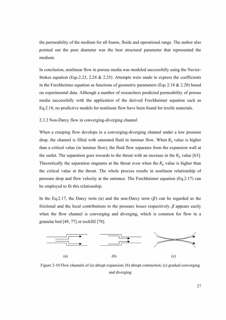
(a) (b) (c)

Figure 2-10 Flow channels of (a) abrupt expansion; (b) abrupt contraction; (c) gradual converging

and diverging

28

When a Newtonian fluid flows in a converging-diverging channel, research on pressure

loss begins from the abrupt changes of flow area as shown in Fig.2.10. Abdelall [79]

investigated pressure losses caused by abrupt flow area expansion and contraction in small

circular channels experimentally, using air and water at room temperature and near

atmospheric pressure. The author found the total and irreversible pressure drops by

applying one dimensional momentum and mechanical energy conservation equations. The

expansion and contraction pressure losses were given by:

∆ = (1 − ) (2-26a)

∆ = ( 1 − + 1 − ( ) ) (2-26b)

Where is the inlet area and is the outlet area, is the contraction coefficient which

is a function of area ratio and . Single-phase flow experiments showed the expansion

and contraction loss coefficient were different for gas and liquid, and with the exception of

the contraction loss coefficient for water they agreed reasonably with the predictions. The

contraction loss coefficients for water were slightly larger than theoretical predictions.

Astarita [80] reported an early experimental study for the case of a sharp-edged

contraction flow channel, and experimental data showed that excess pressure drop was

much larger than published predictions over the entire range of values. Kfuri [81]

studied non-Newtonian fluids flow in abrupt contraction piping systems and addressed the

pressure losses resulting from wall friction, change in the flow direction and in the cross

section of the duct. After numerical simulations, the author constructed equations for the

friction loss coefficient as a function of and the relevant dimensionless rheological

parameter of the non-Newtonian fluid. Pinho [82] carried out a numerical investigation to

study laminar non-Newtonian flow through an axisymmetric sudden expansion tube. The

author found the local loss coefficient was a function of of the inlet pipe.

Thauvin [83] developed a pore level network model to describe high velocity flow in the

near well-bore region and to understand non-Darcy flow behaviour. The inputs to the

model are parameters such as pore size distribution and fluid properties. The outputs are

permeability, non-Darcy coefficient, tortuousity and porosity. The additional pressure

29

gradient term is found to be proportional to the square of the velocity in accordance with

the Forchheimer equation. The correlation between the non-Darcy coefficient and other

flow properties ( ,Ф& ) is found to depend on geometric parameters. The author

separated the pressure loss into viscous (∆ ), bending (∆ ), expansion (∆ ) and

contraction (∆ ) pressure losses. The converging-diverging nature of the pores in porous

media led to inertial pressure losses which are:

∆ = 1 − (2-27a)

∆ = (1.45 − 0.45 − ) (2-27b)

Where is the radius of the throat between the two bodies, is the body radius and is

the average interstitial velocity in the throat. The author discussed the non-Darcy effect

with . After experimental observation, it was found that the pressure gradient is

proportional to the velocity for < 0.11. As the superficial velocity and thus increase,

the relationship between the pressure gradient and velocity becomes nonlinear. At high

values, the pressure gradient is almost proportional to the square of the velocity. Based on

this observation, Zeng [84] recommended a criterion based on the value for non-Darcy

flow in porous media. After experimental determination for nitrogen flow in sandstone, the

critical transition from Darcy flow to non-Darcy flow was suggested to be at =0.11.

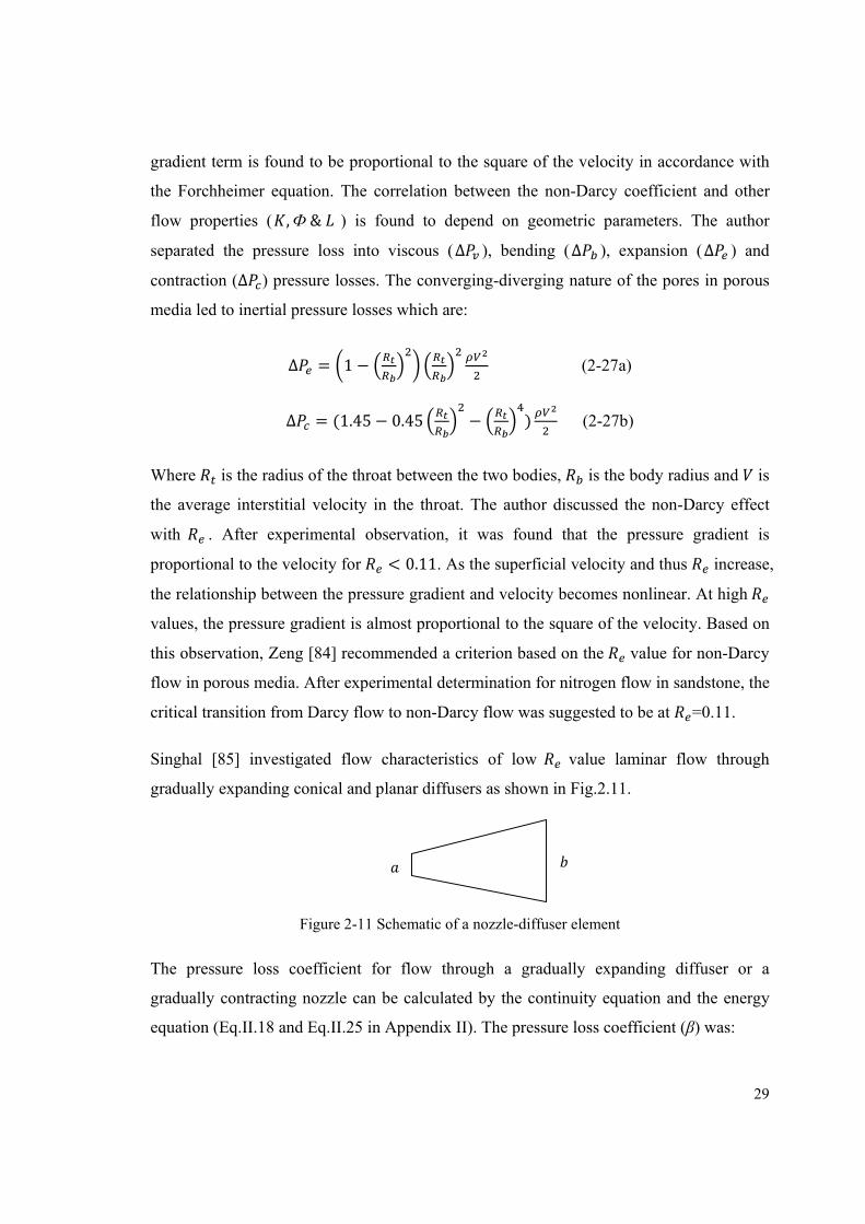
Singhal [85] investigated flow characteristics of low value laminar flow through

gradually expanding conical and planar diffusers as shown in Fig.2.11.

Figure 2-11 Schematic of a nozzle-diffuser element

The pressure loss coefficient for flow through a gradually expanding diffuser or a

gradually contracting nozzle can be calculated by the continuity equation and the energy

equation (Eq.II.18 and Eq.II.25 in Appendix II). The pressure loss coefficient (β) was:

30

= + (1 − ) (2-28)

As ∝ , the expressions for β of conical ( ) and planar ( ) diffusers were:

= + (1 − ) (2-29a)

= + (1 − ) (2-29b)

Where and , and are the static pressures and flow velocities at the cross-

sections a and b, and are the diameters at the cross-sections a and b. The model was

verified by numerical simulations and experimental values, giving reasonable agreement

between the predicted and the experimental results. However, the predictions for pressure

loss were lower in general.

Martin [86] carried out a numerical study of fluid flow around periodic cylinder arrays

under laminar cross flow conditions, considering square and triangular arrays. The study

showed the frictional losses followed Darcy’s law when is of the order of one, while

significant non-Darcy effects were observed at higher . Qu [87, 88] investigated

Newtonian flow development and pressure drop experimentally and computationally for

single phase water flow in a rectangular micro-channel. The author also derived a

nonlinear relationship of pressure loss and flow velocity, containing frictional, contraction

and expansion pressure losses, which had the same style within Eq.2.28. The

computational model showed very good predictions for the measured velocity field and

pressure drop. Sidiropoulou [89] focused on the determination of the Forchheimer

equation coefficients and for non-Darcy flow in a porous medium. The author

evaluated theoretical equations and proposed empirical relations based on the investigation

of available data in the literature. A suggestion was given that the coefficients and

were not constants but depended on the flow velocity, i.e. the value. There were

deviations approximately 10% for the coefficient . A plausible explanation for the

dependence of and on was that the position for which the boundary layer

separation occurred, and subsequently the characteristics of the recirculation zone,

depended on [90]. The paper reviewed Lao’s work [91] and demonstrated on a

31

macroscopic scale, the coefficient was related to energy losses in a straight pipe, i.e.

Poiseuille’s law, and the inertial coefficient depended on minor losses induced at pipe

junctions.

In summary, the flow path in a porous medium might not be regular, such as in a ceramic

material or a granular bed. However, flow in the gaps between yarns in a woven fabric will

experience gradual converging-diverging channels. Reviews of non-Darcy flow in a

sudden [79] or a conical [85] converging-diverging channel provide a useful reference for

the development of a non-Darcy flow model in woven fabrics. Numerical simulation [86,

87] and experimental studies [89] on the Darcy and non-Darcy coefficients provide insight

to the developed model for textile fabrics.

2.4 FABRIC DEFORMATION UNDER UNIFORM LOAD

When a woven fabric is loaded, for example in airbag inflation, the fabric undergoes out-

of-plane deformation under a high pressure load. The load gives the fabric a change in

geometry, especially the gap between yarns and yarn fibre volume fraction, which

influence the fabric permeability significantly. Therefore, an approach to characterize and

describe the fabric deformation under constant and transient pressures is required, based

either on analytical modelling or experimental determination. The change of fabric

geometric parameters such as gap size or yarn width is also required.

During the airbag inflation, pressure drop through the airbag fabric is transient. This

relates to the concept of dynamic permeability. This permeability is obtained during fabric

deformation and transient pressure. A method to determine this fabric permeability is

required in this work.

2.4.1 Dynamic permeability tester

The concept of a dynamic permeability tester has been introduced by several researchers.

Partridge [92] reported a dynamic gas-permeability tester for air-bags commercially made

by Textest Instruments as shown in Fig.2.12.

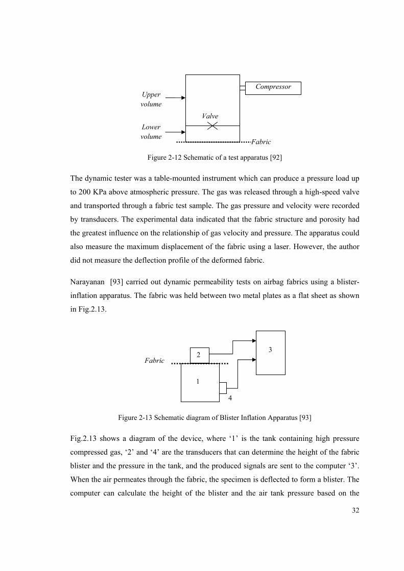
32

Figure 2-12 Schematic of a test apparatus [92]

The dynamic tester was a table-mounted instrument which can produce a pressure load up

to 200 KPa above atmospheric pressure. The gas was released through a high-speed valve

and transported through a fabric test sample. The gas pressure and velocity were recorded

by transducers. The experimental data indicated that the fabric structure and porosity had

the greatest influence on the relationship of gas velocity and pressure. The apparatus could

also measure the maximum displacement of the fabric using a laser. However, the author

did not measure the deflection profile of the deformed fabric.

Narayanan [93] carried out dynamic permeability tests on airbag fabrics using a blister-

inflation apparatus. The fabric was held between two metal plates as a flat sheet as shown

in Fig.2.13.

Figure 2-13 Schematic diagram of Blister Inflation Apparatus [93]

Fig.2.13 shows a diagram of the device, where ‘1’ is the tank containing high pressure

compressed gas, ‘2’ and ‘4’ are the transducers that can determine the height of the fabric

blister and the pressure in the tank, and the produced signals are sent to the computer ‘3’.

When the air permeates through the fabric, the specimen is deflected to form a blister. The

computer can calculate the height of the blister and the air tank pressure based on the

4

1

23

Fabric

Compressor

Valve

Upper volume

Lower volume

Fabric

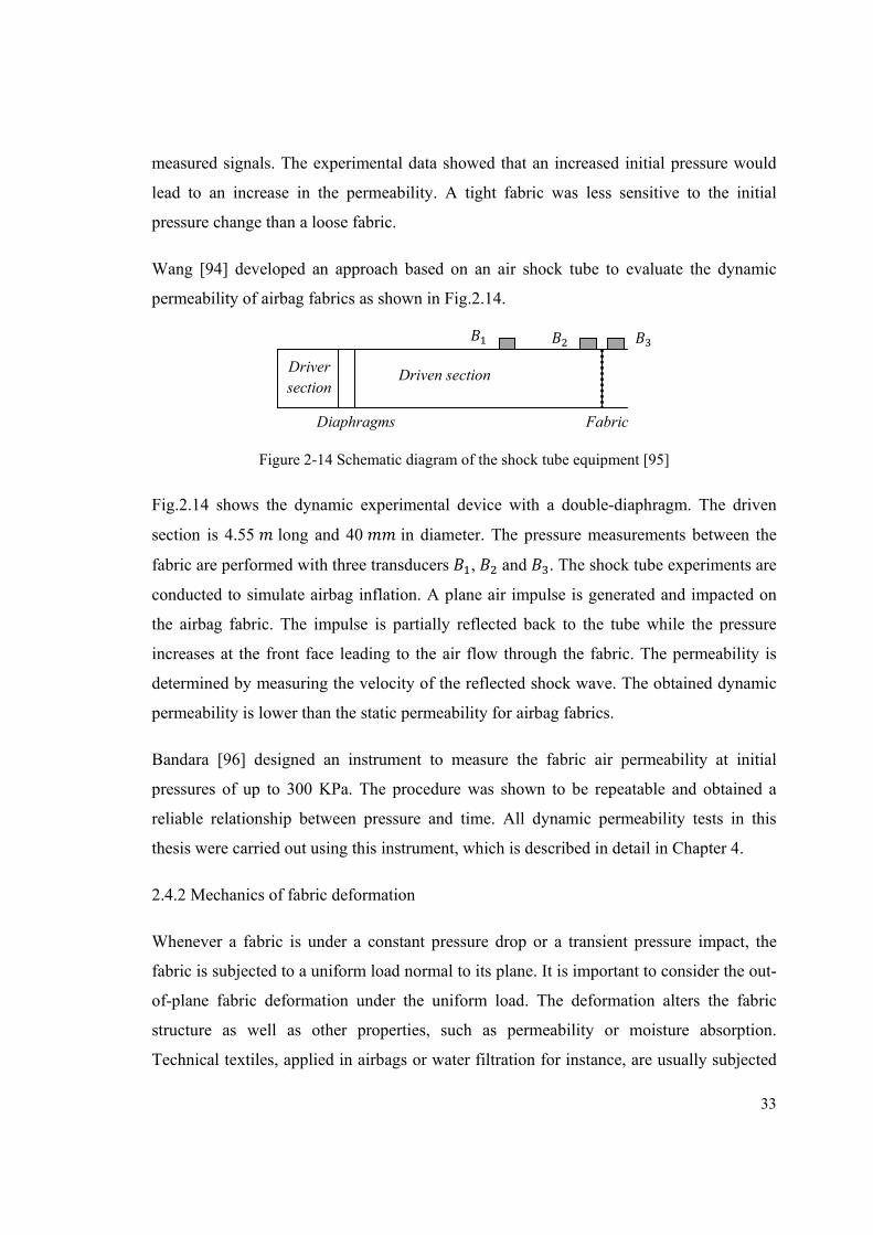
33

measured signals. The experimental data showed that an increased initial pressure would

lead to an increase in the permeability. A tight fabric was less sensitive to the initial

pressure change than a loose fabric.

Wang [94] developed an approach based on an air shock tube to evaluate the dynamic

permeability of airbag fabrics as shown in Fig.2.14.

Figure 2-14 Schematic diagram of the shock tube equipment [95]

Fig.2.14 shows the dynamic experimental device with a double-diaphragm. The driven

section is 4.55 long and 40 in diameter. The pressure measurements between the

fabric are performed with three transducers , and . The shock tube experiments are

conducted to simulate airbag inflation. A plane air impulse is generated and impacted on

the airbag fabric. The impulse is partially reflected back to the tube while the pressure

increases at the front face leading to the air flow through the fabric. The permeability is

determined by measuring the velocity of the reflected shock wave. The obtained dynamic

permeability is lower than the static permeability for airbag fabrics.

Bandara [96] designed an instrument to measure the fabric air permeability at initial

pressures of up to 300 KPa. The procedure was shown to be repeatable and obtained a

reliable relationship between pressure and time. All dynamic permeability tests in this

thesis were carried out using this instrument, which is described in detail in Chapter 4.

2.4.2 Mechanics of fabric deformation

Whenever a fabric is under a constant pressure drop or a transient pressure impact, the

fabric is subjected to a uniform load normal to its plane. It is important to consider the out-

of-plane fabric deformation under the uniform load. The deformation alters the fabric

structure as well as other properties, such as permeability or moisture absorption.

Technical textiles, applied in airbags or water filtration for instance, are usually subjected

Driver section

Driven section

Diaphragms Fabric

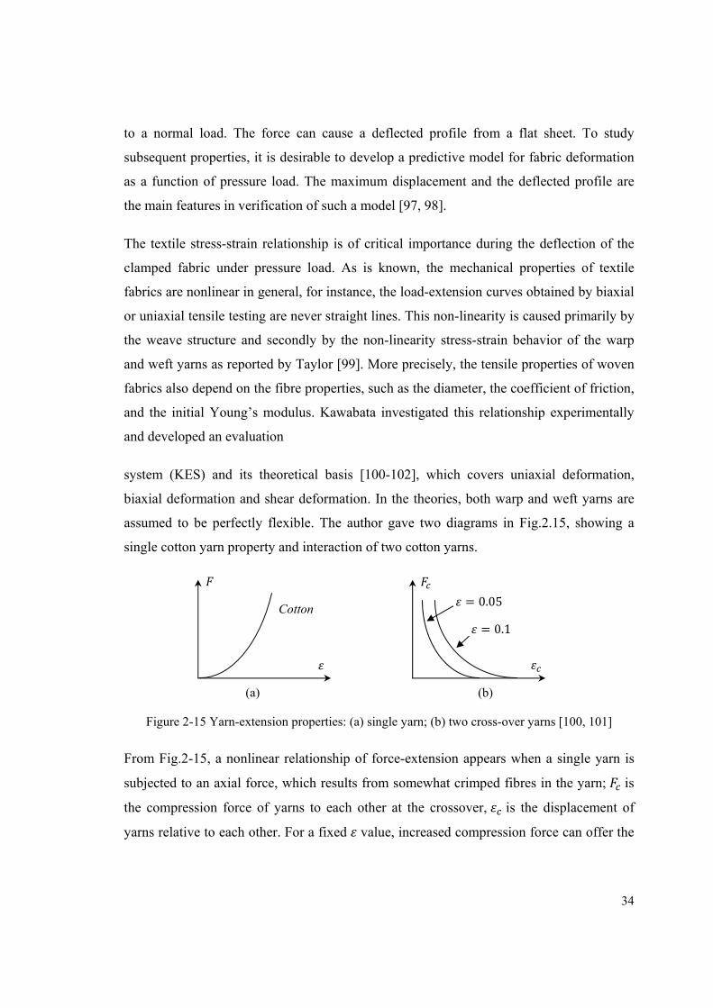
34

to a normal load. The force can cause a deflected profile from a flat sheet. To study

subsequent properties, it is desirable to develop a predictive model for fabric deformation

as a function of pressure load. The maximum displacement and the deflected profile are

the main features in verification of such a model [97, 98].

The textile stress-strain relationship is of critical importance during the deflection of the

clamped fabric under pressure load. As is known, the mechanical properties of textile

fabrics are nonlinear in general, for instance, the load-extension curves obtained by biaxial

or uniaxial tensile testing are never straight lines. This non-linearity is caused primarily by

the weave structure and secondly by the non-linearity stress-strain behavior of the warp

and weft yarns as reported by Taylor [99]. More precisely, the tensile properties of woven

fabrics also depend on the fibre properties, such as the diameter, the coefficient of friction,

and the initial Young’s modulus. Kawabata investigated this relationship experimentally

and developed an evaluation

system (KES) and its theoretical basis [100-102], which covers uniaxial deformation,

biaxial deformation and shear deformation. In the theories, both warp and weft yarns are

assumed to be perfectly flexible. The author gave two diagrams in Fig.2.15, showing a

single cotton yarn property and interaction of two cotton yarns.

(a) (b)

Figure 2-15 Yarn-extension properties: (a) single yarn; (b) two cross-over yarns [100, 101]

From Fig.2-15, a nonlinear relationship of force-extension appears when a single yarn is

subjected to an axial force, which results from somewhat crimped fibres in the yarn; is

the compression force of yarns to each other at the crossover, is the displacement of

yarns relative to each other. For a fixed value, increased compression force can offer the

Cotton

= 0.05= 0.1

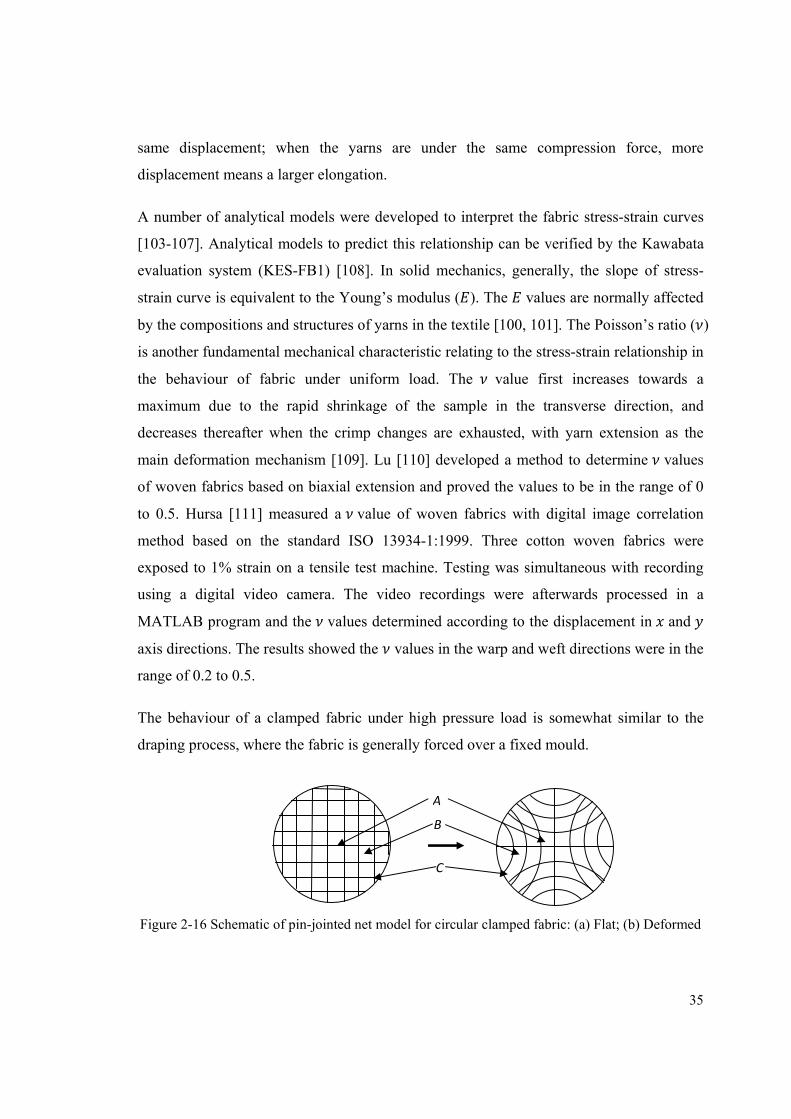
35

same displacement; when the yarns are under the same compression force, more

displacement means a larger elongation.

A number of analytical models were developed to interpret the fabric stress-strain curves

[103-107]. Analytical models to predict this relationship can be verified by the Kawabata

evaluation system (KES-FB1) [108]. In solid mechanics, generally, the slope of stress-

strain curve is equivalent to the Young’s modulus ( ). The values are normally affected

by the compositions and structures of yarns in the textile [100, 101]. The Poisson’s ratio ( )

is another fundamental mechanical characteristic relating to the stress-strain relationship in

the behaviour of fabric under uniform load. The value first increases towards a

maximum due to the rapid shrinkage of the sample in the transverse direction, and

decreases thereafter when the crimp changes are exhausted, with yarn extension as the

main deformation mechanism [109]. Lu [110] developed a method to determine values

of woven fabrics based on biaxial extension and proved the values to be in the range of 0

to 0.5. Hursa [111] measured a value of woven fabrics with digital image correlation

method based on the standard ISO 13934-1:1999. Three cotton woven fabrics were

exposed to 1% strain on a tensile test machine. Testing was simultaneous with recording

using a digital video camera. The video recordings were afterwards processed in a

MATLAB program and the values determined according to the displacement in and

axis directions. The results showed the values in the warp and weft directions were in the

range of 0.2 to 0.5.

The behaviour of a clamped fabric under high pressure load is somewhat similar to the

draping process, where the fabric is generally forced over a fixed mould.

Figure 2-16 Schematic of pin-jointed net model for circular clamped fabric: (a) Flat; (b) Deformed

C

B

A

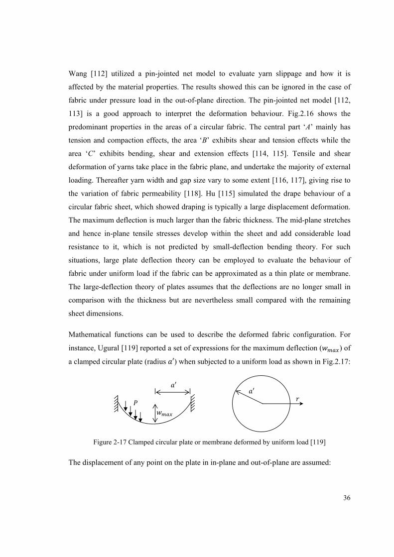
36

Wang [112] utilized a pin-jointed net model to evaluate yarn slippage and how it is

affected by the material properties. The results showed this can be ignored in the case of

fabric under pressure load in the out-of-plane direction. The pin-jointed net model [112,

113] is a good approach to interpret the deformation behaviour. Fig.2.16 shows the

predominant properties in the areas of a circular fabric. The central part ‘A’ mainly has

tension and compaction effects, the area ‘B’ exhibits shear and tension effects while the

area ‘C’ exhibits bending, shear and extension effects [114, 115]. Tensile and shear

deformation of yarns take place in the fabric plane, and undertake the majority of external

loading. Thereafter yarn width and gap size vary to some extent [116, 117], giving rise to

the variation of fabric permeability [118]. Hu [115] simulated the drape behaviour of a

circular fabric sheet, which showed draping is typically a large displacement deformation.

The maximum deflection is much larger than the fabric thickness. The mid-plane stretches

and hence in-plane tensile stresses develop within the sheet and add considerable load

resistance to it, which is not predicted by small-deflection bending theory. For such

situations, large plate deflection theory can be employed to evaluate the behaviour of

fabric under uniform load if the fabric can be approximated as a thin plate or membrane.

The large-deflection theory of plates assumes that the deflections are no longer small in

comparison with the thickness but are nevertheless small compared with the remaining

sheet dimensions.

Mathematical functions can be used to describe the deformed fabric configuration. For

instance, Ugural [119] reported a set of expressions for the maximum deflection ( ) of

a clamped circular plate (radius ′) when subjected to a uniform load as shown in Fig.2.17:

Figure 2-17 Clamped circular plate or membrane deformed by uniform load [119]

The displacement of any point on the plate in in-plane and out-of-plane are assumed:

′ ′

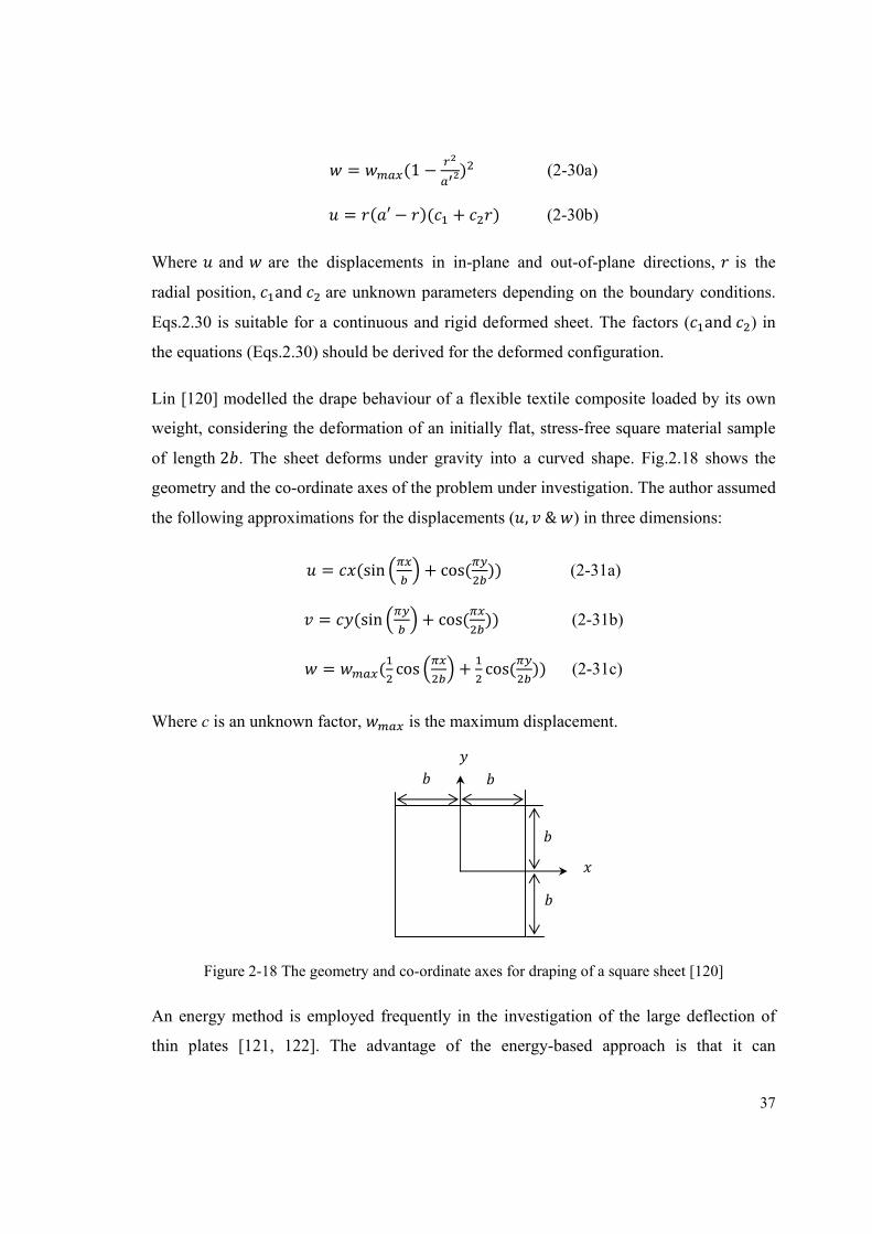
37

= (1 − ) (2-30a) = ( ′ − )( + ) (2-30b)

Where and are the displacements in in-plane and out-of-plane directions, is the

radial position, and are unknown parameters depending on the boundary conditions.

Eqs.2.30 is suitable for a continuous and rigid deformed sheet. The factors ( and ) in

the equations (Eqs.2.30) should be derived for the deformed configuration.

Lin [120] modelled the drape behaviour of a flexible textile composite loaded by its own

weight, considering the deformation of an initially flat, stress-free square material sample

of length 2 . The sheet deforms under gravity into a curved shape. Fig.2.18 shows the

geometry and the co-ordinate axes of the problem under investigation. The author assumed

the following approximations for the displacements ( , & ) in three dimensions:

= (sin + cos( )) (2-31a)

= (sin + cos( )) (2-31b)

= ( cos + cos( )) (2-31c)

Where c is an unknown factor, is the maximum displacement.

Figure 2-18 The geometry and co-ordinate axes for draping of a square sheet [120]

An energy method is employed frequently in the investigation of the large deflection of

thin plates [121, 122]. The advantage of the energy-based approach is that it can

38

incorporate the material nonlinearity as well as geometric nonlinearities, which are

characteristic features of fabric sheet mechanics problems. Lin assumed that the tensile

energy ( ) of the plate consists of the energy of stretching ( ∬( + ) )

and the energy of shearing ( ∬ ). The definition is given by [119]:

= ∬( + + ) (2-32)

Where , are normal forces per unit distance on and planes, , are normal

strains in and directions, and is shear strain in the plane. Bending energy ( )

is defined as [119]:

= ∬ ( + ) − (1 − ) − ( ) (2-33)

Where is the area of the plate surface, is the displacement in the out-of-plane direction,

is the plate Poisson’s ratio, D is the flexural rigidity. When a fabric plate undergoes a

normal load, the work done ( ) by the surface force per unit area on the fabric from the

initial to the equilibrium state is expressed as:

= ∬ (2-34)

Therefore the total deformation energy ( Π) of the system is the sum of the bending

energy, the membrane energy and the work done:

Π = + + (2-35)

In which, relates bending strain energy, which concerns with out-of-plane deformation;

links membrane strain energy to the fabric Young’s modulus, which concerns in-plane

deformation; denotes the work done by the uniformly distributed pressure load. Then,

application of the minimizing condition, Π = 0, yields approximate expressions for

the maximum deflection and out-of plane displacement of the sheet [119]. The

mathematical predictions for maximum deflections had good agreement with predictions

by finite element simulations.

39

Based on the energy minimization method, King [123] proposed a continuum constitutive

model for predicting fabric mechanical behaviour in the planar direction. The approach

relied on selection of a geometric model for the fabric weave, coupled with constitutive

models for the yarn behaviour. The structural configuration was related to the macroscopic

deformation. Finite element analysis and experimental findings showed good agreement

with predictions for fabric in-plane loading. However, the model was not evaluated for

fabric deformation under out-of-plane loading.

2.5 CONCLUSIONS

After review of relevant published work, it is noted that there has been much research on

the permeability of porous media analytically, numerically and experimentally. However

for one-layer or 3D woven fabrics, no model can predict the permeabilities accurately

without fitting factors. When a Newtonian fluid flows through the gaps between yarns in a

woven fabric with small , the gaps actually form a set of gradual converging-diverging

flow channels, which cannot be regarded as straight tubes (the Kulichenko model). If the

flow goes through the yarns, many models such as the Kozeny and the Gebart models have

considered flow along and perpendicular to the fibre bundles with their existing limitations,

for instance a fitting factor in the Kozeny model and a shape factor in the Gebart model.

Moreover, in real textiles, yarns usually follow an undulating path, and no model considers

this factor. Therefore, a unified permeability model for both gap flow (loose fabric) and

yarn flow (tight fabric) is required. Fortunately, many reviewed methodologies, such as the

lubrication approach, can be explored to develop permeability models for woven fabric.

The Forchheimer equation in porous media has been reviewed. Many non-linear empirical

equations of this style have been reviewed for different porous media, and some hints can

be obtained for woven fabrics, which are often subjected to flow of high so that a

nonlinear relationship of pressure drop and fluid velocity appears. As no model can

explain the fluid behaviour through the converging-diverging gaps in a woven fabric under

high pressure, an analytical model is required to predict the Darcy coefficient as well as

the non-Darcy coefficient in this situation.

40

When a woven fabric is subjected to a high pressure load, such as a fabric in airbag

inflation, its original structure and permeability will be changed. As textile fabric is

discontinuous and anisotropic, the energy approach (based on the reviewed previous work)

can be used to model fabric deformation. As no model has been found for fabric

permeability under pressure load, an analytical model is desired to predict the variation of

geometric factors inside the woven fabric and its subsequent permeability under pressure

load.

41

CHAPTER 3

MODELLING OF FABRIC STATIC PERMEABILITY

3.1 INTRODUCTION

The main aim of developing the static permeability model for woven fabric is to predict

the through-thickness permeability by taking into account different geometric factors such

as fabric layers, yarn cross-section shape, fibre volume fraction, fibre arrangement etc. As

stated in Chapter 1, static permeability can be obtained by Darcy’s law when fabrics are

under small value and constant pressure drop by experiment. The analytical model is

thereafter verified by the experimental data. An accurate predictive analytical model for

fabric static permeability can help manufacturers to design fabrics with improved

properties before extensive and expensive prototyping. Engineers can predict how fabric

will behave under different conditions and modify the configuration to suit the specific

application.

This chapter develops a predictive through-thickness permeability model for different

types of woven fabrics. It is a unified permeability model for one-layer of woven fabric

considering flow through gaps between yarns and space inside yarns. The gap between

yarns is assumed as a gradual converging-diverging flow channel for which all geometric

factors can be obtained experimentally. The subsequent gap permeability is developed

based on the lubrication approach analogous to the Gebart model [22]. The yarn

permeability is, however, a combination of the Gebart model [22] and the Advani model

[124], which describes flow through an undulating yarn including flow along and

perpendicular to its fibres. Therefore, the model takes into account two structural

components i.e. the gap between yarns and the porous yarns. With emphasis on flow

channel geometry, characterization of fabric structure is critical to successful prediction.

Permeability of 3D woven fabric is derived as a function of the permeability of each fabric

layer. In this chapter, analytical models for one-layer and 3D woven fabrics are verified by

numerical simulations and experimental tests.

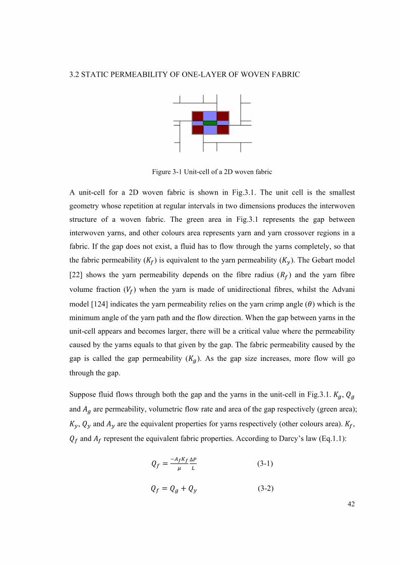
42

3.2 STATIC PERMEABILITY OF ONE-LAYER OF WOVEN FABRIC

Figure 3-1 Unit-cell of a 2D woven fabric

A unit-cell for a 2D woven fabric is shown in Fig.3.1. The unit cell is the smallest

geometry whose repetition at regular intervals in two dimensions produces the interwoven

structure of a woven fabric. The green area in Fig.3.1 represents the gap between

interwoven yarns, and other colours area represents yarn and yarn crossover regions in a

fabric. If the gap does not exist, a fluid has to flow through the yarns completely, so that

the fabric permeability ( ) is equivalent to the yarn permeability ( ). The Gebart model

[22] shows the yarn permeability depends on the fibre radius ( ) and the yarn fibre

volume fraction ( ) when the yarn is made of unidirectional fibres, whilst the Advani

model [124] indicates the yarn permeability relies on the yarn crimp angle ( ) which is the

minimum angle of the yarn path and the flow direction. When the gap between yarns in the

unit-cell appears and becomes larger, there will be a critical value where the permeability

caused by the yarns equals to that given by the gap. The fabric permeability caused by the

gap is called the gap permeability ( ). As the gap size increases, more flow will go

through the gap.

Suppose fluid flows through both the gap and the yarns in the unit-cell in Fig.3.1. ,

and are permeability, volumetric flow rate and area of the gap respectively (green area);

, and are the equivalent properties for yarns respectively (other colours area). ,

and represent the equivalent fabric properties. According to Darcy’s law (Eq.1.1):

= ∆ (3-1)

= + (3-2)

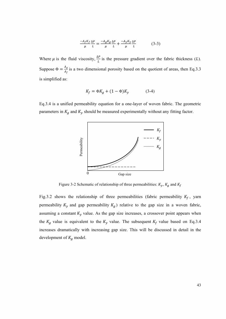
43

∆ = ∆ + ∆ (3-3)

Where is the fluid viscosity, ∆

is the pressure gradient over the fabric thickness ( ).

Suppose Ф = is a two dimensional porosity based on the quotient of areas, then Eq.3.3

is simplified as: = Ф + (1 − Ф) (3-4)

Eq.3.4 is a unified permeability equation for a one-layer of woven fabric. The geometric

parameters in and should be measured experimentally without any fitting factor.

Figure 3-2 Schematic of relationship of three permeabilities: , and

Fig.3.2 shows the relationship of three permeabilities (fabric permeability , yarn

permeability and gap permeability ) relative to the gap size in a woven fabric,

assuming a constant value. As the gap size increases, a crossover point appears when

the value is equivalent to the value. The subsequent value based on Eq.3.4

increases dramatically with increasing gap size. This will be discussed in detail in the

development of model.

Gap size

Per

mea

bili

ty

0

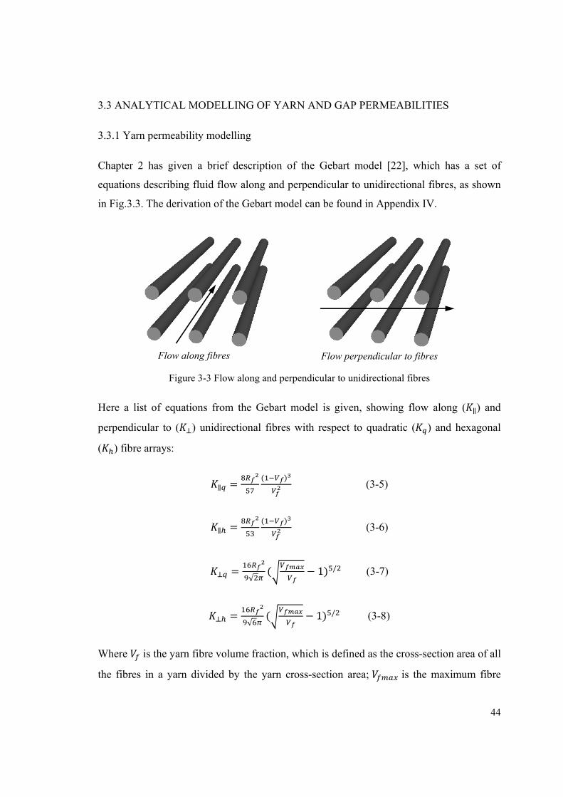
44

3.3 ANALYTICAL MODELLING OF YARN AND GAP PERMEABILITIES

3.3.1 Yarn permeability modelling

Chapter 2 has given a brief description of the Gebart model [22], which has a set of

equations describing fluid flow along and perpendicular to unidirectional fibres, as shown

in Fig.3.3. The derivation of the Gebart model can be found in Appendix IV.

Figure 3-3 Flow along and perpendicular to unidirectional fibres

Here a list of equations from the Gebart model is given, showing flow along ( ∥) and

perpendicular to ( ) unidirectional fibres with respect to quadratic ( ) and hexagonal

( ) fibre arrays:

∥ = ( ) (3-5)

∥ = ( ) (3-6)

= √ ( − 1) / (3-7)

= √ ( − 1) / (3-8)

Where is the yarn fibre volume fraction, which is defined as the cross-section area of all

the fibres in a yarn divided by the yarn cross-section area; is the maximum fibre

Flow along fibres Flow perpendicular to fibres

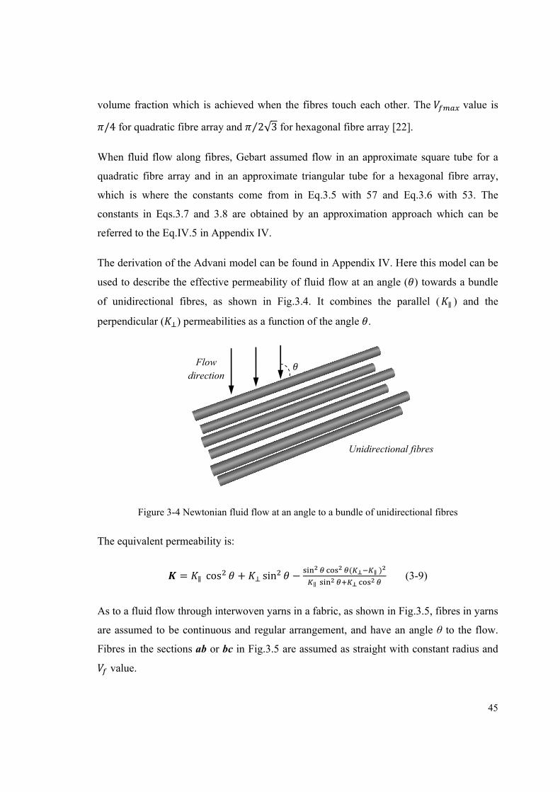
45

volume fraction which is achieved when the fibres touch each other. The value is /4 for quadratic fibre array and 2√3⁄ for hexagonal fibre array [22].

When fluid flow along fibres, Gebart assumed flow in an approximate square tube for a

quadratic fibre array and in an approximate triangular tube for a hexagonal fibre array,

which is where the constants come from in Eq.3.5 with 57 and Eq.3.6 with 53. The

constants in Eqs.3.7 and 3.8 are obtained by an approximation approach which can be

referred to the Eq.IV.5 in Appendix IV.

The derivation of the Advani model can be found in Appendix IV. Here this model can be

used to describe the effective permeability of fluid flow at an angle ( ) towards a bundle

of unidirectional fibres, as shown in Fig.3.4. It combines the parallel ( ∥ ) and the

perpendicular ( ) permeabilities as a function of the angle .

Figure 3-4 Newtonian fluid flow at an angle to a bundle of unidirectional fibres

The equivalent permeability is:

= ∥ cos + sin − ( ∥)∥ (3-9)

As to a fluid flow through interwoven yarns in a fabric, as shown in Fig.3.5, fibres in yarns

are assumed to be continuous and regular arrangement, and have an angle θ to the flow.

Fibres in the sections ab or bc in Fig.3.5 are assumed as straight with constant radius and

value.

Flow direction

Unidirectional fibres

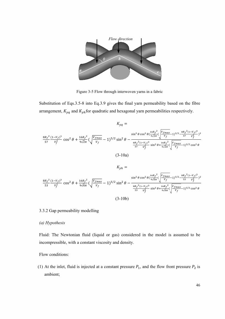
46

Figure 3-5 Flow through interwoven yarns in a fabric

Substitution of Eqs.3.5-8 into Eq.3.9 gives the final yarn permeability based on the fibre

arrangement, and for quadratic and hexagonal yarn permeabilities respectively.

=( ) cos + √ ( − 1) / sin − ( √ ( ) / ( ) )

( ) √ ( ) /

(3-10a)

=( ) cos + √ ( − 1) / sin − ( √ ( ) / ( ) )

( ) √ ( ) /

(3-10b)

3.3.2 Gap permeability modelling

(a) Hypothesis

Fluid: The Newtonian fluid (liquid or gas) considered in the model is assumed to be

incompressible, with a constant viscosity and density.

Flow conditions:

(1) At the inlet, fluid is injected at a constant pressure , and the flow front pressure is

ambient;

Flow direction

a

b

c

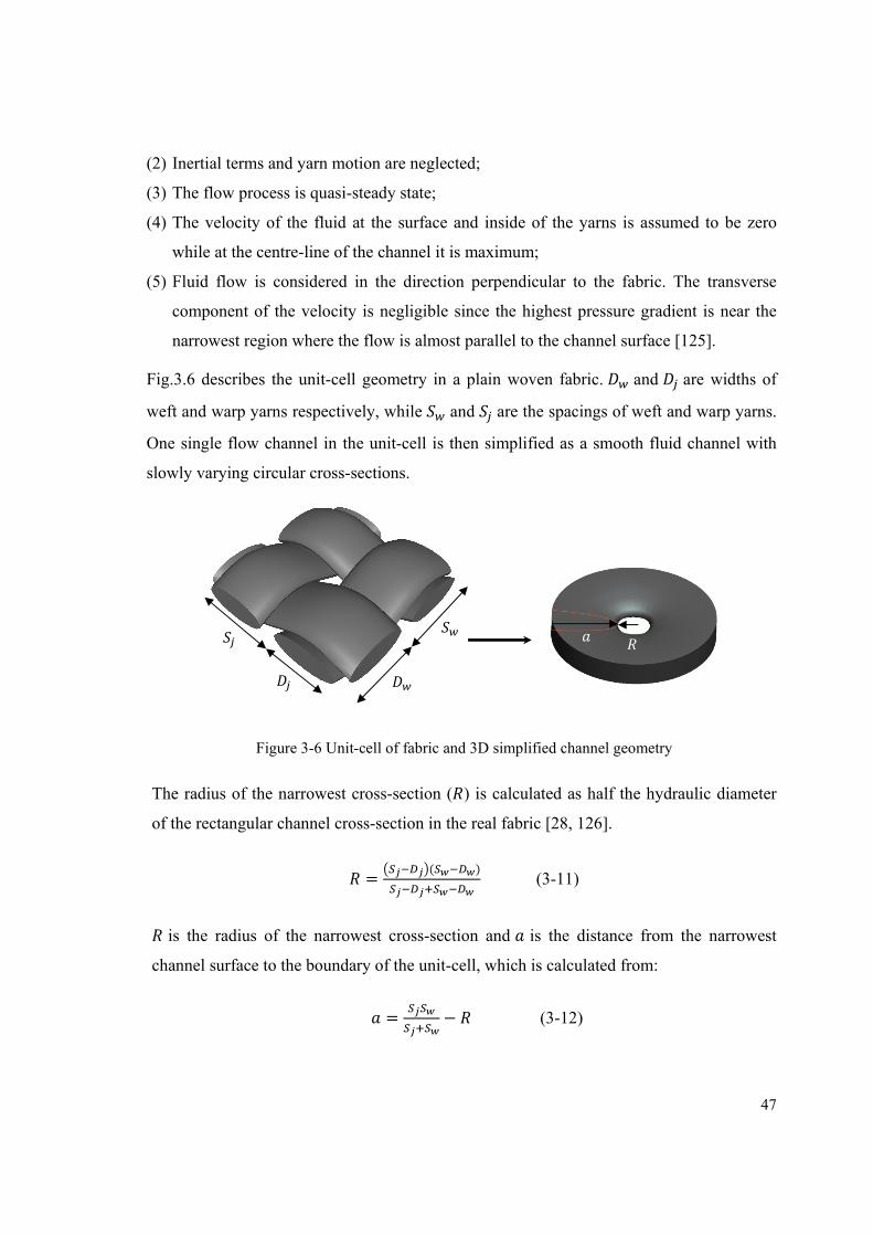
47

(2) Inertial terms and yarn motion are neglected;

(3) The flow process is quasi-steady state;

(4) The velocity of the fluid at the surface and inside of the yarns is assumed to be zero

while at the centre-line of the channel it is maximum;

(5) Fluid flow is considered in the direction perpendicular to the fabric. The transverse

component of the velocity is negligible since the highest pressure gradient is near the

narrowest region where the flow is almost parallel to the channel surface [125].

Fig.3.6 describes the unit-cell geometry in a plain woven fabric. and are widths of

weft and warp yarns respectively, while and are the spacings of weft and warp yarns.

One single flow channel in the unit-cell is then simplified as a smooth fluid channel with

slowly varying circular cross-sections.

Figure 3-6 Unit-cell of fabric and 3D simplified channel geometry

The radius of the narrowest cross-section ( ) is calculated as half the hydraulic diameter

of the rectangular channel cross-section in the real fabric [28, 126].

= ( ) (3-11)

is the radius of the narrowest cross-section and is the distance from the narrowest

channel surface to the boundary of the unit-cell, which is calculated from:

= − (3-12)

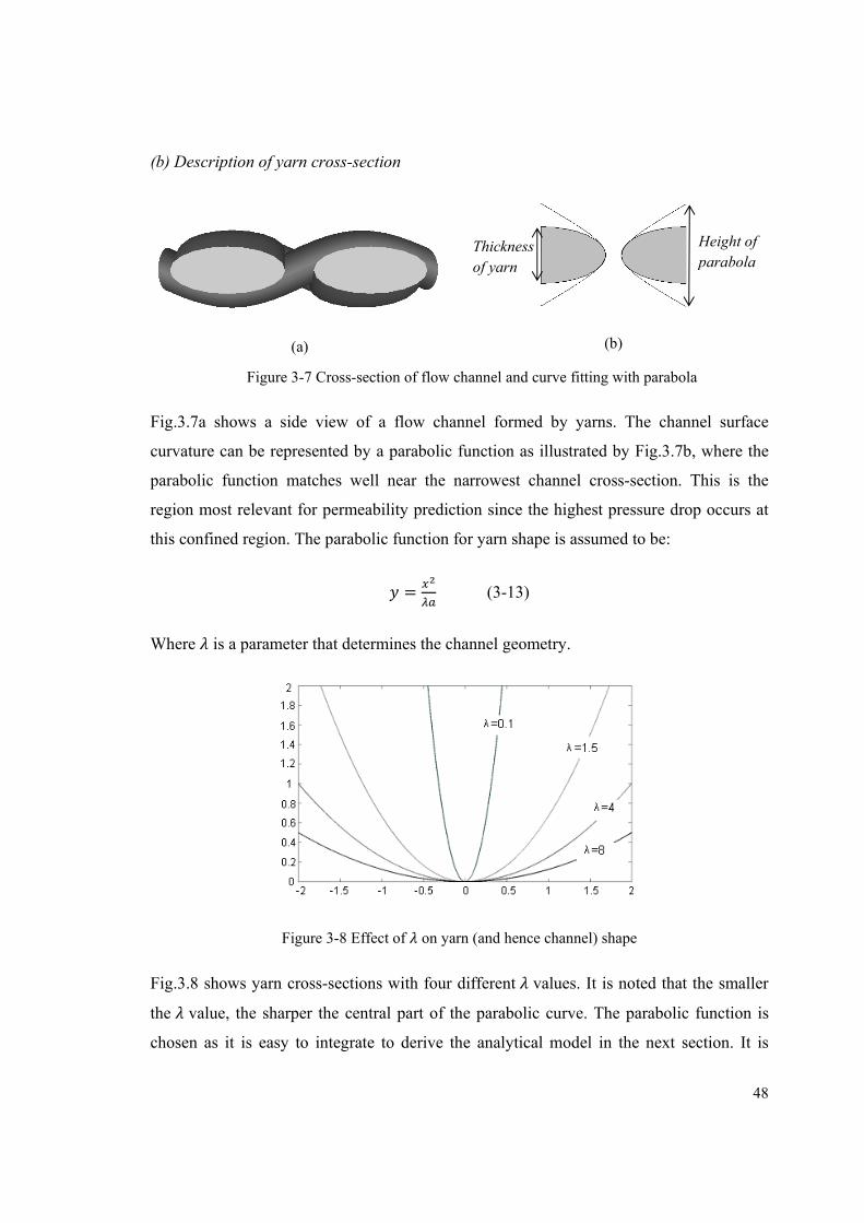
48

(b) Description of yarn cross-section

Figure 3-7 Cross-section of flow channel and curve fitting with parabola

Fig.3.7a shows a side view of a flow channel formed by yarns. The channel surface

curvature can be represented by a parabolic function as illustrated by Fig.3.7b, where the

parabolic function matches well near the narrowest channel cross-section. This is the

region most relevant for permeability prediction since the highest pressure drop occurs at

this confined region. The parabolic function for yarn shape is assumed to be:

= (3-13)

Where is a parameter that determines the channel geometry.

Figure 3-8 Effect of on yarn (and hence channel) shape

Fig.3.8 shows yarn cross-sections with four different values. It is noted that the smaller

the value, the sharper the central part of the parabolic curve. The parabolic function is

chosen as it is easy to integrate to derive the analytical model in the next section. It is

Thickness of yarn

Height of parabola

(a) (b)

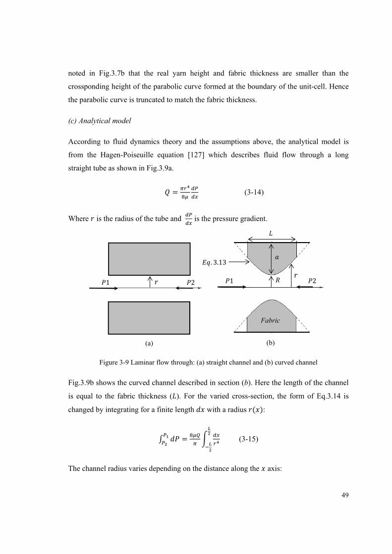
49

noted in Fig.3.7b that the real yarn height and fabric thickness are smaller than the

crossponding height of the parabolic curve formed at the boundary of the unit-cell. Hence

the parabolic curve is truncated to match the fabric thickness.

(c) Analytical model

According to fluid dynamics theory and the assumptions above, the analytical model is

from the Hagen-Poiseuille equation [127] which describes fluid flow through a long

straight tube as shown in Fig.3.9a.

= (3-14)

Where is the radius of the tube and is the pressure gradient.

Figure 3-9 Laminar flow through: (a) straight channel and (b) curved channel

Fig.3.9b shows the curved channel described in section (b). Here the length of the channel

is equal to the fabric thickness ( ). For the varied cross-section, the form of Eq.3.14 is

changed by integrating for a finite length with a radius ( ): = (3-15)

The channel radius varies depending on the distance along the axis:

(a) (b)

. 3.13

Fabric

1 2

21

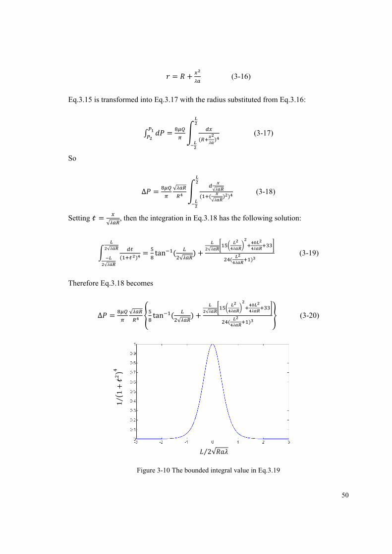
50

= + (3-16)

Eq.3.15 is transformed into Eq.3.17 with the radius substituted from Eq.3.16:

= ( ) (3-17)

So

∆ = √ √( (√ ) ) (3-18)

Setting = √ , then the integration in Eq.3.18 has the following solution:

( )√√ = tan ( √ ) + √ ( ) (3-19)

Therefore Eq.3.18 becomes

∆ = √ tan ( √ ) + √ ( ) (3-20)

Figure 3-10 The bounded integral value in Eq.3.19

2√⁄

11+⁄

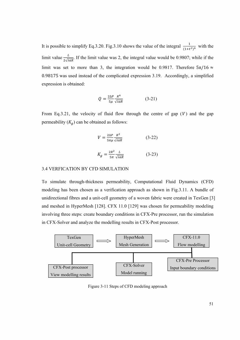
51

It is possible to simplify Eq.3.20. Fig.3.10 shows the value of the integral ( ) with the

limit value √ . If the limit value was 2, the integral value would be 0.9807; while if the

limit was set to more than 3, the integration would be 0.9817. Therefore 5π/16 ≈0.98175 was used instead of the complicated expression 3.19. Accordingly, a simplified

expression is obtained:

= ∆ √ (3-21)

From Eq.3.21, the velocity of fluid flow through the centre of gap ( ) and the gap

permeability ( ) can be obtained as follows:

= ∆ √ (3-22)

= √ (3-23)

3.4 VERFICATION BY CFD SIMULATION

To simulate through-thickness permeability, Computational Fluid Dynamics (CFD)

modeling has been chosen as a verification approach as shown in Fig.3.11. A bundle of

unidirectional fibres and a unit-cell geometry of a woven fabric were created in TexGen [3]

and meshed in HyperMesh [128]. CFX 11.0 [129] was chosen for permeability modeling

involving three steps: create boundary conditions in CFX-Pre processor, run the simulation

in CFX-Solver and analyze the modelling results in CFX-Post processor.

Figure 3-11 Steps of CFD modeling approach

TexGen

Unit-cell Geometry

HyperMesh

Mesh Generation

CFX-11.0

Flow modelling

CFX-Pre Processor

Input boundary conditions CFX-Solver

Model running CFX-Post processor

View modelling results

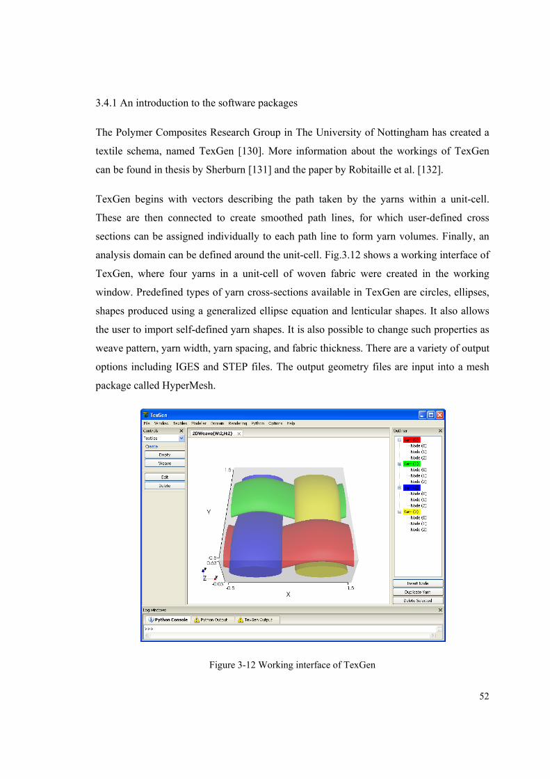
52

3.4.1 An introduction to the software packages

The Polymer Composites Research Group in The University of Nottingham has created a

textile schema, named TexGen [130]. More information about the workings of TexGen

can be found in thesis by Sherburn [131] and the paper by Robitaille et al. [132].

TexGen begins with vectors describing the path taken by the yarns within a unit-cell.

These are then connected to create smoothed path lines, for which user-defined cross

sections can be assigned individually to each path line to form yarn volumes. Finally, an

analysis domain can be defined around the unit-cell. Fig.3.12 shows a working interface of

TexGen, where four yarns in a unit-cell of woven fabric were created in the working

window. Predefined types of yarn cross-sections available in TexGen are circles, ellipses,

shapes produced using a generalized ellipse equation and lenticular shapes. It also allows

the user to import self-defined yarn shapes. It is also possible to change such properties as

weave pattern, yarn width, yarn spacing, and fabric thickness. There are a variety of output

options including IGES and STEP files. The output geometry files are input into a mesh

package called HyperMesh.

Figure 3-12 Working interface of TexGen

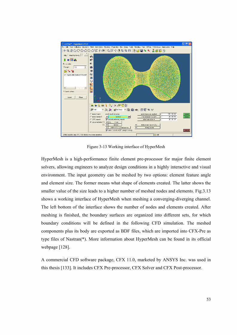
53

Figure 3-13 Working interface of HyperMesh

HyperMesh is a high-performance finite element pre-processor for major finite element

solvers, allowing engineers to analyze design conditions in a highly interactive and visual

environment. The input geometry can be meshed by two options: element feature angle

and element size. The former means what shape of elements created. The latter shows the

smaller value of the size leads to a higher number of meshed nodes and elements. Fig.3.13

shows a working interface of HyperMesh when meshing a converging-diverging channel.

The left bottom of the interface shows the number of nodes and elements created. After

meshing is finished, the boundary surfaces are organized into different sets, for which

boundary conditions will be defined in the following CFD simulation. The meshed

components plus its body are exported as BDF files, which are imported into CFX-Pre as

type files of Nastran(*). More information about HyperMesh can be found in its official

webpage [128].

A commercial CFD software package, CFX 11.0, marketed by ANSYS Inc. was used in

this thesis [133]. It includes CFX Pre-processor, CFX Solver and CFX Post-processor.

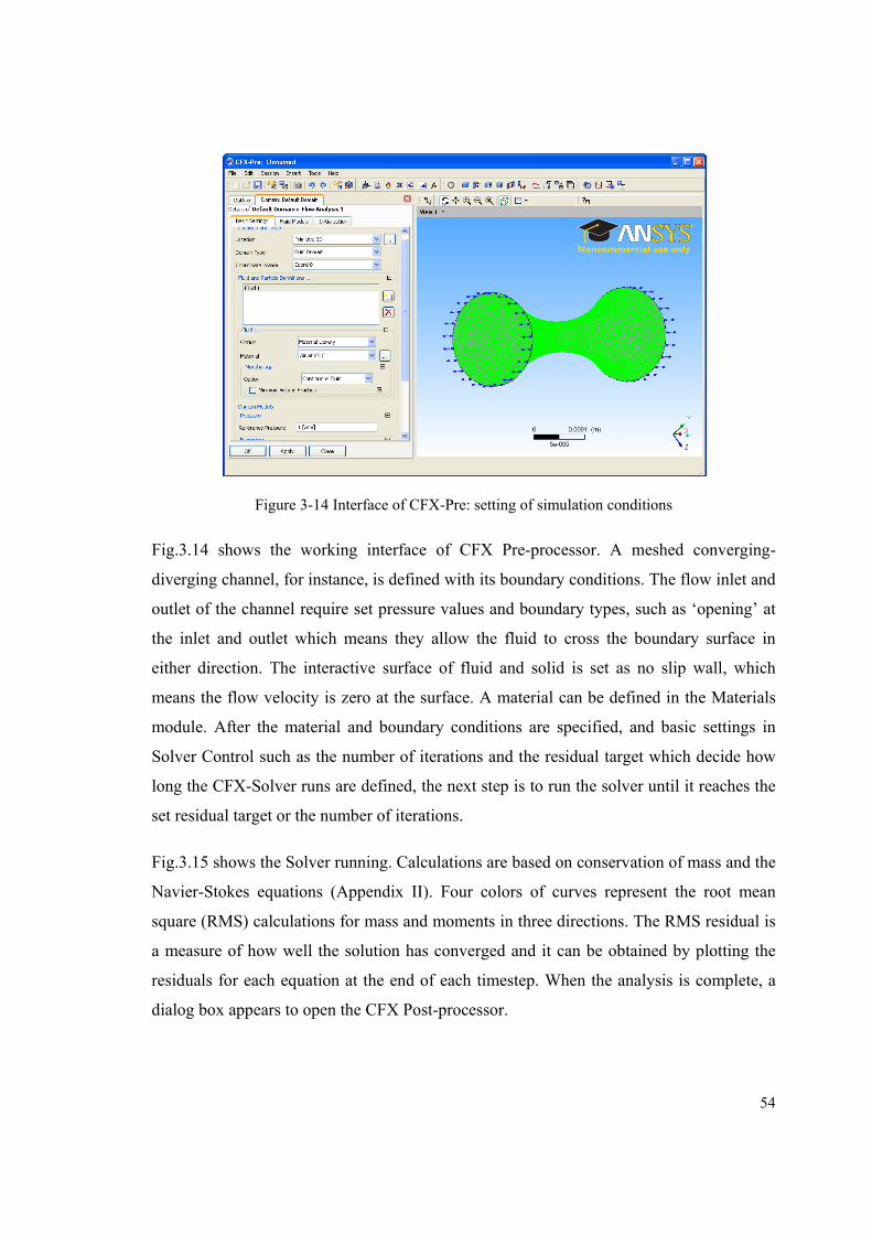
54

Figure 3-14 Interface of CFX-Pre: setting of simulation conditions

Fig.3.14 shows the working interface of CFX Pre-processor. A meshed converging-

diverging channel, for instance, is defined with its boundary conditions. The flow inlet and

outlet of the channel require set pressure values and boundary types, such as ‘opening’ at

the inlet and outlet which means they allow the fluid to cross the boundary surface in

either direction. The interactive surface of fluid and solid is set as no slip wall, which

means the flow velocity is zero at the surface. A material can be defined in the Materials

module. After the material and boundary conditions are specified, and basic settings in

Solver Control such as the number of iterations and the residual target which decide how

long the CFX-Solver runs are defined, the next step is to run the solver until it reaches the

set residual target or the number of iterations.

Fig.3.15 shows the Solver running. Calculations are based on conservation of mass and the

Navier-Stokes equations (Appendix II). Four colors of curves represent the root mean

square (RMS) calculations for mass and moments in three directions. The RMS residual is

a measure of how well the solution has converged and it can be obtained by plotting the

residuals for each equation at the end of each timestep. When the analysis is complete, a

dialog box appears to open the CFX Post-processor.

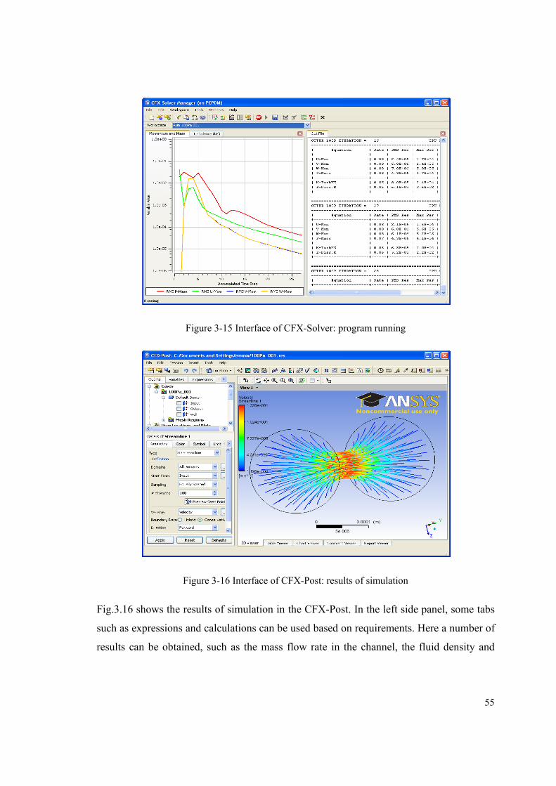
55

Figure 3-15 Interface of CFX-Solver: program running

Figure 3-16 Interface of CFX-Post: results of simulation

Fig.3.16 shows the results of simulation in the CFX-Post. In the left side panel, some tabs

such as expressions and calculations can be used based on requirements. Here a number of

results can be obtained, such as the mass flow rate in the channel, the fluid density and

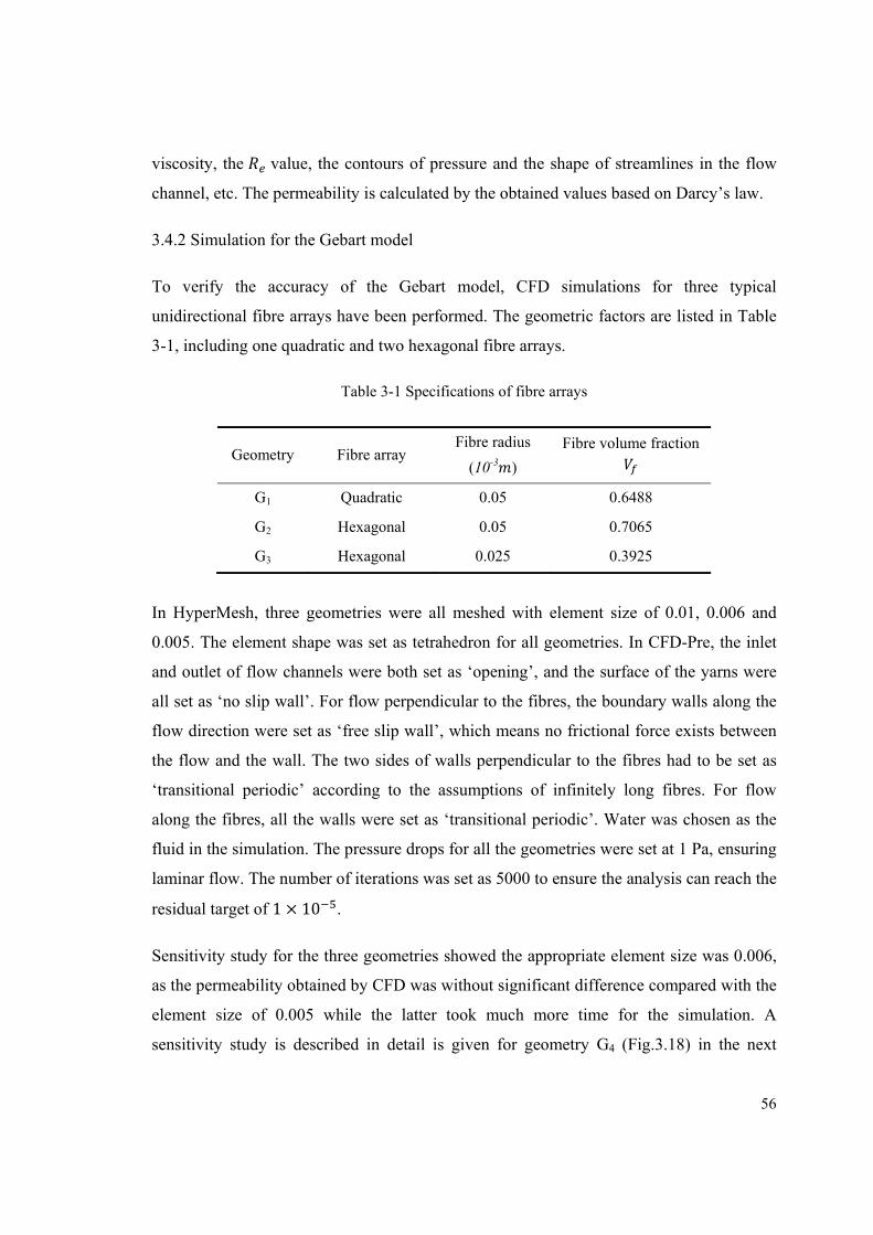
56

viscosity, the value, the contours of pressure and the shape of streamlines in the flow

channel, etc. The permeability is calculated by the obtained values based on Darcy’s law.

3.4.2 Simulation for the Gebart model

To verify the accuracy of the Gebart model, CFD simulations for three typical

unidirectional fibre arrays have been performed. The geometric factors are listed in Table

3-1, including one quadratic and two hexagonal fibre arrays.

Table 3-1 Specifications of fibre arrays

Geometry Fibre array Fibre radius

(10-3 )

Fibre volume fraction

G1 Quadratic 0.05 0.6488

G2 Hexagonal 0.05 0.7065

G3 Hexagonal 0.025 0.3925

In HyperMesh, three geometries were all meshed with element size of 0.01, 0.006 and

0.005. The element shape was set as tetrahedron for all geometries. In CFD-Pre, the inlet

and outlet of flow channels were both set as ‘opening’, and the surface of the yarns were

all set as ‘no slip wall’. For flow perpendicular to the fibres, the boundary walls along the

flow direction were set as ‘free slip wall’, which means no frictional force exists between

the flow and the wall. The two sides of walls perpendicular to the fibres had to be set as

‘transitional periodic’ according to the assumptions of infinitely long fibres. For flow

along the fibres, all the walls were set as ‘transitional periodic’. Water was chosen as the

fluid in the simulation. The pressure drops for all the geometries were set at 1 Pa, ensuring

laminar flow. The number of iterations was set as 5000 to ensure the analysis can reach the

residual target of 1 × 10 .

Sensitivity study for the three geometries showed the appropriate element size was 0.006,

as the permeability obtained by CFD was without significant difference compared with the

element size of 0.005 while the latter took much more time for the simulation. A

sensitivity study is described in detail is given for geometry G4 (Fig.3.18) in the next

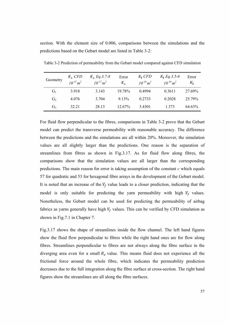
57

section. With the element size of 0.006, comparisons between the simulations and the

predictions based on the Gebart model are listed in Table 3-2:

Table 3-2 Prediction of permeability from the Gebart model compared against CFD simulation

Geometry CFD

10-12 m2

Eq.3.7-8

10-12 m2

Error

∥ CFD

10-10 m2

∥ Eq.3.5-6

10-10 m2

Error ∥ G1 3.918 3.143 19.78% 0.4994 0.3611 27.69%

G2 4.076 3.704 9.13% 0.2733 0.2028 25.79%

G3 32.21 28.13 12.67% 3.4301 1.373 64.63%

For fluid flow perpendicular to the fibres, comparisons in Table 3-2 prove that the Gebart

model can predict the transverse permeability with reasonable accuracy. The difference

between the predictions and the simulations are all within 20%. Moreover, the simulation

values are all slightly larger than the predictions. One reason is the separation of

streamlines from fibres as shown in Fig.3.17. As for fluid flow along fibres, the

comparisons show that the simulation values are all larger than the corresponding

predictions. The main reason for error is taking assumption of the constant c which equals

57 for quadratic and 53 for hexagonal fibre arrays in the development of the Gebart model.

It is noted that an increase of the value leads to a closer prediction, indicating that the

model is only suitable for predicting the yarn permeability with high values.

Nonetheless, the Gebart model can be used for predicting the permeability of airbag

fabrics as yarns generally have high values. This can be verified by CFD simulation as

shown in Fig.7.1 in Chapter 7.

Fig.3.17 shows the shape of streamlines inside the flow channel. The left hand figures

show the fluid flow perpendicular to fibres while the right hand ones are for flow along

fibres. Streamlines perpendicular to fibres are not always along the fibre surface in the

diverging area even for a small value. This means fluid does not experience all the

frictional force around the whole fibre, which indicates the permeability prediction

decreases due to the full integration along the fibre surface at cross-section. The right hand

figures show the streamlines are all along the fibre surfaces.

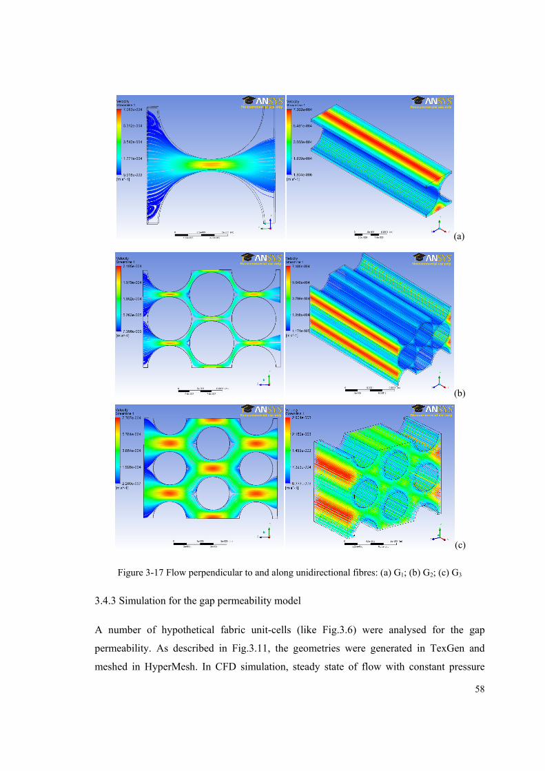
58

(a)

(b)

(c)

Figure 3-17 Flow perpendicular to and along unidirectional fibres: (a) G1; (b) G2; (c) G3

3.4.3 Simulation for the gap permeability model

A number of hypothetical fabric unit-cells (like Fig.3.6) were analysed for the gap

permeability. As described in Fig.3.11, the geometries were generated in TexGen and

meshed in HyperMesh. In CFD simulation, steady state of flow with constant pressure

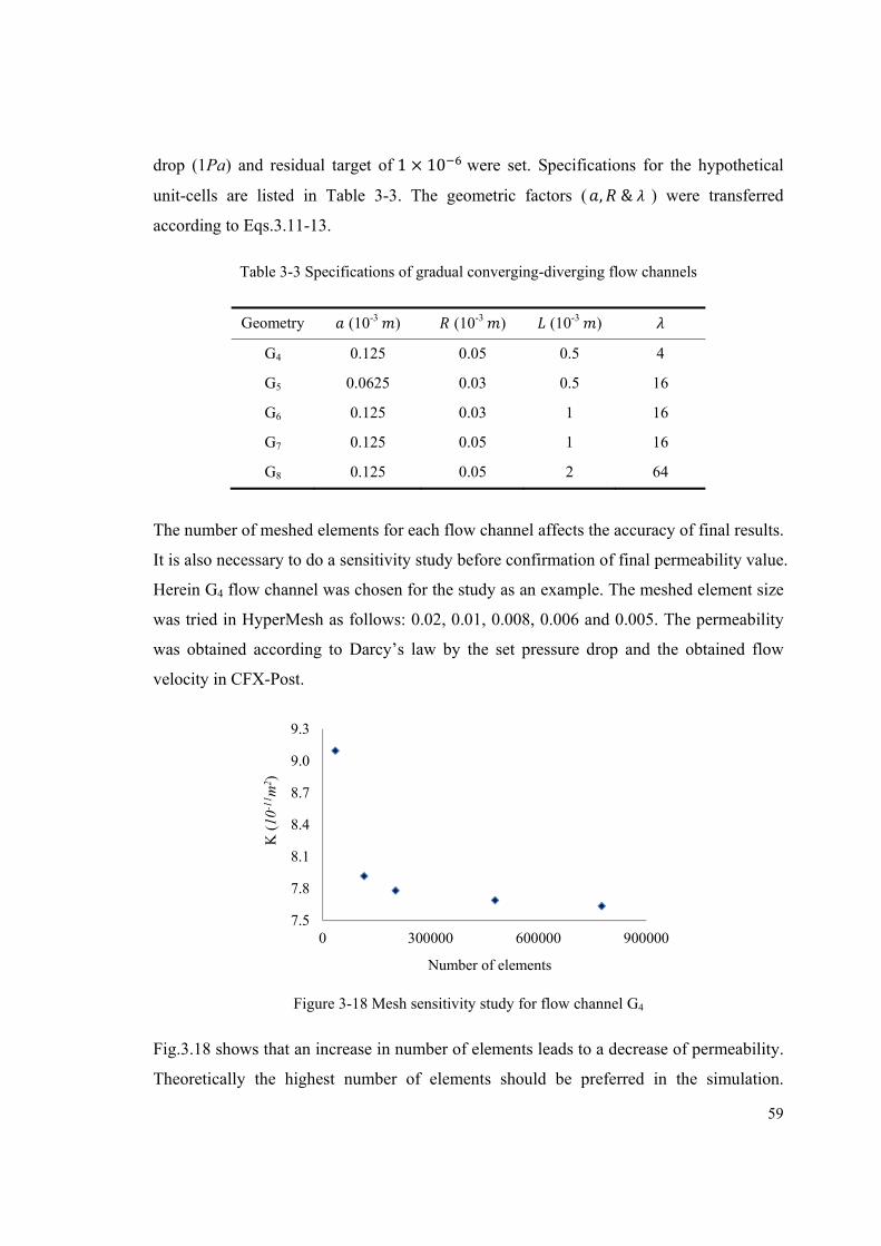
59

drop (1Pa) and residual target of 1 × 10 were set. Specifications for the hypothetical

unit-cells are listed in Table 3-3. The geometric factors ( , & ) were transferred

according to Eqs.3.11-13.

Table 3-3 Specifications of gradual converging-diverging flow channels

Geometry (10-3 ) (10-3 ) (10-3 )

G4 0.125 0.05 0.5 4

G5 0.0625 0.03 0.5 16

G6 0.125 0.03 1 16

G7 0.125 0.05 1 16

G8 0.125 0.05 2 64

The number of meshed elements for each flow channel affects the accuracy of final results.

It is also necessary to do a sensitivity study before confirmation of final permeability value.

Herein G4 flow channel was chosen for the study as an example. The meshed element size

was tried in HyperMesh as follows: 0.02, 0.01, 0.008, 0.006 and 0.005. The permeability

was obtained according to Darcy’s law by the set pressure drop and the obtained flow

velocity in CFX-Post.

Figure 3-18 Mesh sensitivity study for flow channel G4

Fig.3.18 shows that an increase in number of elements leads to a decrease of permeability.

Theoretically the highest number of elements should be preferred in the simulation.

7.5

7.8

8.1

8.4

8.7

9.0

9.3

0 300000 600000 900000

K (

10-1

1 m2 )

Number of elements

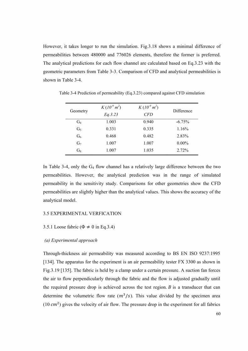
60

However, it takes longer to run the simulation. Fig.3.18 shows a minimal difference of

permeabilities between 480000 and 776026 elements, therefore the former is preferred.

The analytical predictions for each flow channel are calculated based on Eq.3.23 with the

geometric parameters from Table 3-3. Comparison of CFD and analytical permeabilities is

shown in Table 3-4.

Table 3-4 Prediction of permeability (Eq.3.23) compared against CFD simulation

Geometry K (10-9 m2)

Eq.3.23

K (10-9 m2)

CFD Difference

G4 1.003 0.940 -6.75%

G5 0.331 0.335 1.16%

G6 0.468 0.482 2.83%

G7 1.007 1.007 0.00%

G8 1.007 1.035 2.72%

In Table 3-4, only the G4 flow channel has a relatively large difference between the two

permeabilities. However, the analytical prediction was in the range of simulated

permeability in the sensitivity study. Comparisons for other geometries show the CFD

permeabilities are slightly higher than the analytical values. This shows the accuracy of the

analytical model.

3.5 EXPERIMENTAL VERFICATION

3.5.1 Loose fabric (Ф ≠ 0 in Eq.3.4)

(a) Experimental approach

Through-thickness air permeability was measured according to BS EN ISO 9237:1995

[134]. The apparatus for the experiment is an air permeability tester FX 3300 as shown in

Fig.3.19 [135]. The fabric is held by a clamp under a certain pressure. A suction fan forces

the air to flow perpendicularly through the fabric and the flow is adjusted gradually until

the required pressure drop is achieved across the test region. is a transducer that can

determine the volumetric flow rate ( / ). This value divided by the specimen area

(10 ) gives the velocity of air flow. The pressure drop in the experiment for all fabrics

61

is set to 500 Pa, with an accuracy of at least 2%. Using the measured velocity, pressure

drop and fabric thickness, permeability is calculated according to Darcy’s law.

Figure 3-19 Sketch of air permeability tester FX3300

Table 3-5 Fabric specifications [10]

Fabric Composition and Structure

Average

10-6

Yarn

value 10-3

Yarn spacing 10-3

Yarn width

10-3

Warp Sj

Weft Sw

Warp Dj

Weft Dw

U1 100%Cotton Plain 4.3 0.56 0.323 0.470 0.410 0.405 0.279

U2 65/35 PET/Cotton Plain 5.4 0.58 0.319 0.223 0.331 0.184 0.202

C1 67PET/33Cotton

Desized, scoured, bleached and mercerized 2/1twill

5.9 0.56 0.419 0.340 0.480 0.310 0.310

C2 67PET/33Cotton

Dyed, not finished 2/1twill 5.9 0.63 0.425 0.330 0.532 0.300 0.430

C3 67PET/33Cotton Finished 2/1twill

5.5 0.57 0.427 0.300 0.510 0.270 0.330

C7 67PET/33Cotton

Desized, scoured, bleached and mercerized 2/1twill

5.7 0.60 0.452 0.340 0.450 0.300 0.400

C8 67PET/33Cotton Finished 2/1twill

5.7 0.61 0.455 0.340 0.430 0.300 0.350

C9 60Cotton/ 40PET

Same process as C1, 2/2 twill 5.6 0.67 0.560 0.356 0.520 0.332 0.450

C10 60Cotton/ 40PET Finished

2/2twill 5.7 0.56 0.610 0.342 0.446 0.313 0.380

B Fabric Air

Fan

Clamp

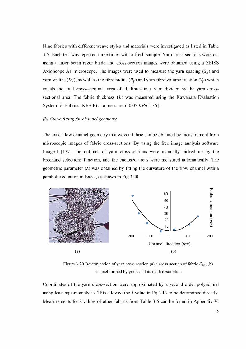
62

Nine fabrics with different weave styles and materials were investigated as listed in Table

3-5. Each test was repeated three times with a fresh sample. Yarn cross-sections were cut

using a laser beam razor blade and cross-section images were obtained using a ZEISS

AxioScope A1 microscope. The images were used to measure the yarn spacing ( ) and

yarn widths ( ), as well as the fibre radius ( ) and yarn fibre volume fraction ( ) which

equals the total cross-sectional area of all fibres in a yarn divided by the yarn cross-

sectional area. The fabric thickness ( ) was measured using the Kawabata Evaluation

System for Fabrics (KES-F) at a pressure of 0.05 KPa [136].

(b) Curve fitting for channel geometry

The exact flow channel geometry in a woven fabric can be obtained by measurement from

microscopic images of fabric cross-sections. By using the free image analysis software

Image-J [137], the outlines of yarn cross-sections were manually picked up by the

Freehand selections function, and the enclosed areas were measured automatically. The

geometric parameter (λ) was obtained by fitting the curvature of the flow channel with a

parabolic equation in Excel, as shown in Fig.3.20.

Figure 3-20 Determination of yarn cross-section (a) a cross-section of fabric ; (b)

channel formed by yarns and its math description

Coordinates of the yarn cross-section were approximated by a second order polynomial

using least square analysis. This allowed the value in Eq.3.13 to be determined directly.

Measurements for values of other fabrics from Table 3-5 can be found in Appendix V.

(a)

Channel direction ( )

Radius direction (

)

(b)

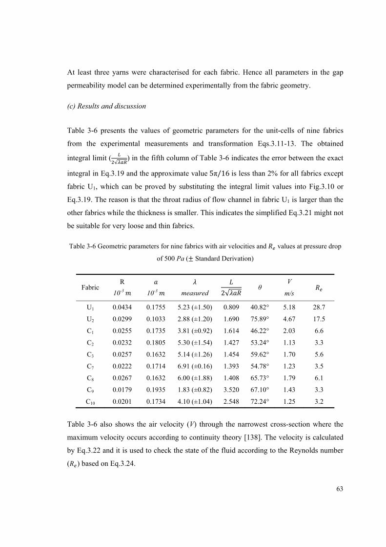
63

At least three yarns were characterised for each fabric. Hence all parameters in the gap

permeability model can be determined experimentally from the fabric geometry.

(c) Results and discussion

Table 3-6 presents the values of geometric parameters for the unit-cells of nine fabrics

from the experimental measurements and transformation Eqs.3.11-13. The obtained

integral limit ( √ ) in the fifth column of Table 3-6 indicates the error between the exact

integral in Eq.3.19 and the approximate value 5π/16 is less than 2% for all fabrics except

fabric U1, which can be proved by substituting the integral limit values into Fig.3.10 or

Eq.3.19. The reason is that the throat radius of flow channel in fabric U1 is larger than the

other fabrics while the thickness is smaller. This indicates the simplified Eq.3.21 might not

be suitable for very loose and thin fabrics.

Table 3-6 Geometric parameters for nine fabrics with air velocities and values at pressure drop

of 500 Pa (± Standard Derivation)

Fabric R

10-3

10-3

measured 2√ θ V

m/s

U1 0.0434 0.1755 5.23 (±1.50) 0.809 40.82° 5.18 28.7

U2 0.0299 0.1033 2.88 (±1.20) 1.690 75.89° 4.67 17.5

C1 0.0255 0.1735 3.81 (±0.92) 1.614 46.22° 2.03 6.6

C2 0.0232 0.1805 5.30 (±1.54) 1.427 53.24° 1.13 3.3

C3 0.0257 0.1632 5.14 (±1.26) 1.454 59.62° 1.70 5.6

C7 0.0222 0.1714 6.91 (±0.16) 1.393 54.78° 1.23 3.5

C8 0.0267 0.1632 6.00 (±1.88) 1.408 65.73° 1.79 6.1

C9 0.0179 0.1935 1.83 (±0.82) 3.520 67.10° 1.43 3.3

C10 0.0201 0.1734 4.10 (±1.04) 2.548 72.24° 1.25 3.2

Table 3-6 also shows the air velocity (V) through the narrowest cross-section where the

maximum velocity occurs according to continuity theory [138]. The velocity is calculated

by Eq.3.22 and it is used to check the state of the fluid according to the Reynolds number

( ) based on Eq.3.24.

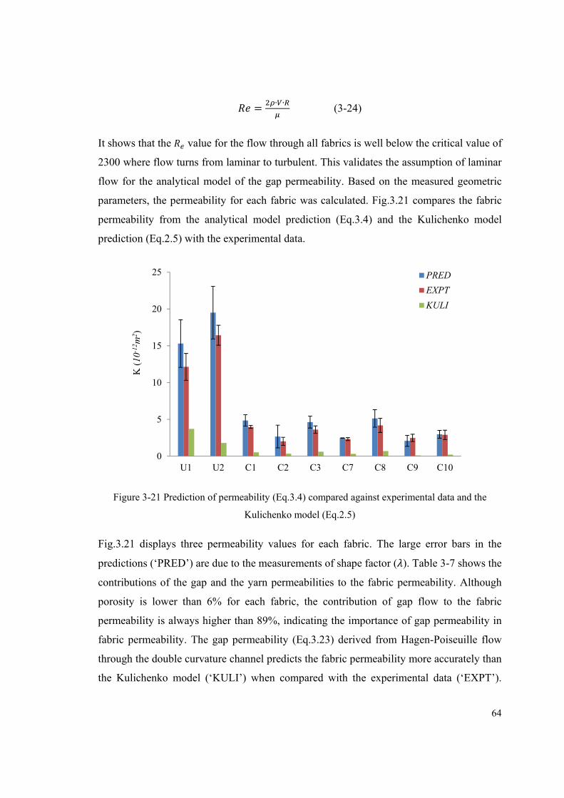
64

= ∙ ∙ (3-24)

It shows that the value for the flow through all fabrics is well below the critical value of

2300 where flow turns from laminar to turbulent. This validates the assumption of laminar

flow for the analytical model of the gap permeability. Based on the measured geometric

parameters, the permeability for each fabric was calculated. Fig.3.21 compares the fabric

permeability from the analytical model prediction (Eq.3.4) and the Kulichenko model

prediction (Eq.2.5) with the experimental data.

Figure 3-21 Prediction of permeability (Eq.3.4) compared against experimental data and the

Kulichenko model (Eq.2.5)

Fig.3.21 displays three permeability values for each fabric. The large error bars in the

predictions (‘PRED’) are due to the measurements of shape factor ( ). Table 3-7 shows the

contributions of the gap and the yarn permeabilities to the fabric permeability. Although

porosity is lower than 6% for each fabric, the contribution of gap flow to the fabric

permeability is always higher than 89%, indicating the importance of gap permeability in

fabric permeability. The gap permeability (Eq.3.23) derived from Hagen-Poiseuille flow

through the double curvature channel predicts the fabric permeability more accurately than

the Kulichenko model (‘KULI’) when compared with the experimental data (‘EXPT’).

0

5

10

15

20

25

U1 U2 C1 C2 C3 C7 C8 C9 C10

K (

10-1

2 m2 )

PRED

EXPT

KULI

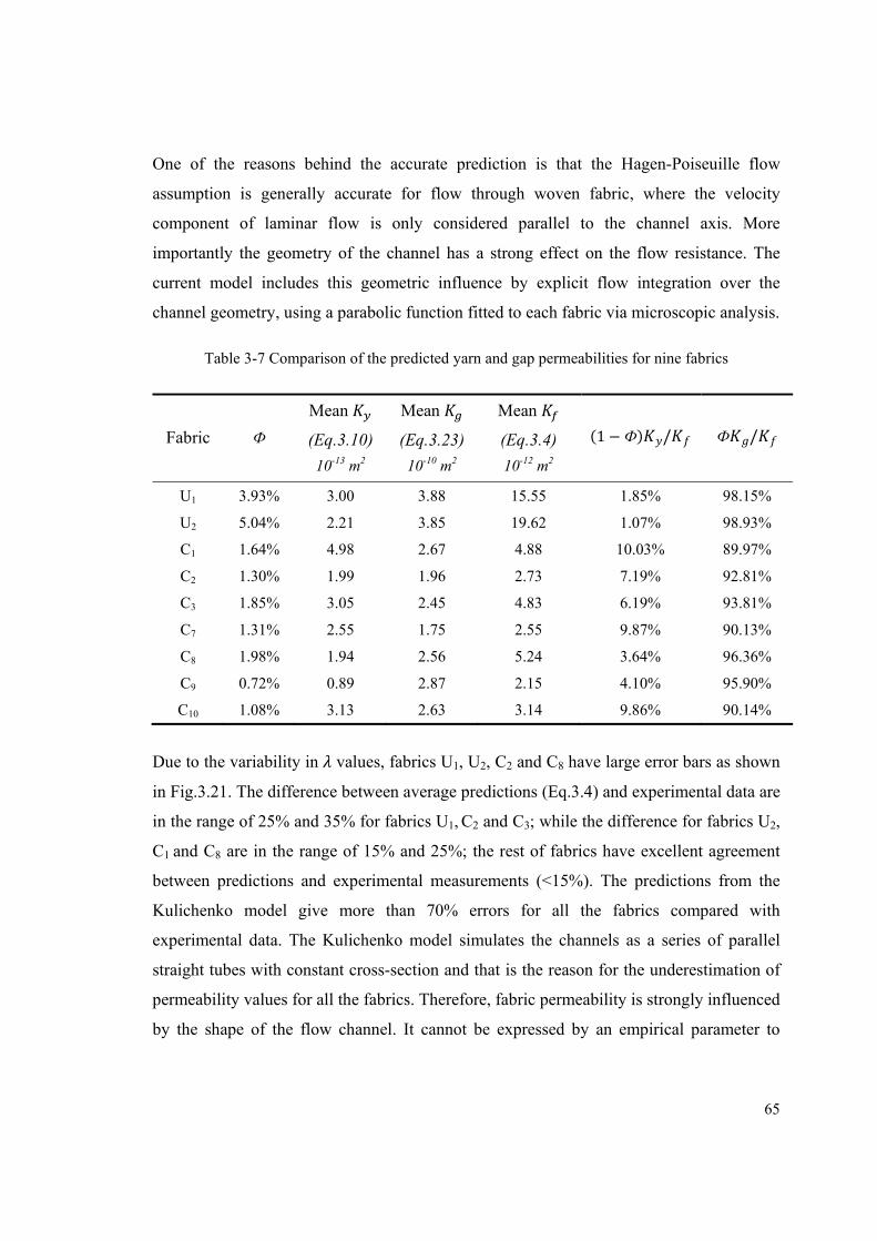
65

One of the reasons behind the accurate prediction is that the Hagen-Poiseuille flow

assumption is generally accurate for flow through woven fabric, where the velocity

component of laminar flow is only considered parallel to the channel axis. More

importantly the geometry of the channel has a strong effect on the flow resistance. The

current model includes this geometric influence by explicit flow integration over the

channel geometry, using a parabolic function fitted to each fabric via microscopic analysis.

Table 3-7 Comparison of the predicted yarn and gap permeabilities for nine fabrics

Fabric Ф

Mean

(Eq.3.10)

10-13 m2

Mean

(Eq.3.23)

10-10 m2

Mean

(Eq.3.4)

10-12 m2

(1 −Ф) / Ф /

U1 3.93% 3.00 3.88 15.55 1.85% 98.15%

U2 5.04% 2.21 3.85 19.62 1.07% 98.93%

C1 1.64% 4.98 2.67 4.88 10.03% 89.97%

C2 1.30% 1.99 1.96 2.73 7.19% 92.81%

C3 1.85% 3.05 2.45 4.83 6.19% 93.81%

C7 1.31% 2.55 1.75 2.55 9.87% 90.13%

C8 1.98% 1.94 2.56 5.24 3.64% 96.36%

C9 0.72% 0.89 2.87 2.15 4.10% 95.90%

C10 1.08% 3.13 2.63 3.14 9.86% 90.14%

Due to the variability in values, fabrics U1, U2, C2 and C8 have large error bars as shown

in Fig.3.21. The difference between average predictions (Eq.3.4) and experimental data are

in the range of 25% and 35% for fabrics U1, C2 and C3; while the difference for fabrics U2,

C1 and C8 are in the range of 15% and 25%; the rest of fabrics have excellent agreement

between predictions and experimental measurements (<15%). The predictions from the

Kulichenko model give more than 70% errors for all the fabrics compared with

experimental data. The Kulichenko model simulates the channels as a series of parallel

straight tubes with constant cross-section and that is the reason for the underestimation of

permeability values for all the fabrics. Therefore, fabric permeability is strongly influenced

by the shape of the flow channel. It cannot be expressed by an empirical parameter to

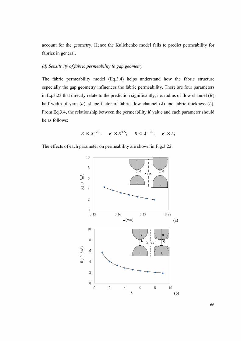
66

account for the geometry. Hence the Kulichenko model fails to predict permeability for

fabrics in general.

(d) Sensitivity of fabric permeability to gap geometry

The fabric permeability model (Eq.3.4) helps understand how the fabric structure

especially the gap geometry influences the fabric permeability. There are four parameters

in Eq.3.23 that directly relate to the prediction significantly, i.e. radius of flow channel ( ),

half width of yarn ( ), shape factor of fabric flow channel ( ) and fabric thickness ( ).

From Eq.3.4, the relationship between the permeability value and each parameter should

be as follows: ∝ . ; ∝ . ; ∝ . ; ∝ ;

The effects of each parameter on permeability are shown in Fig.3.22.

(a)

(b)

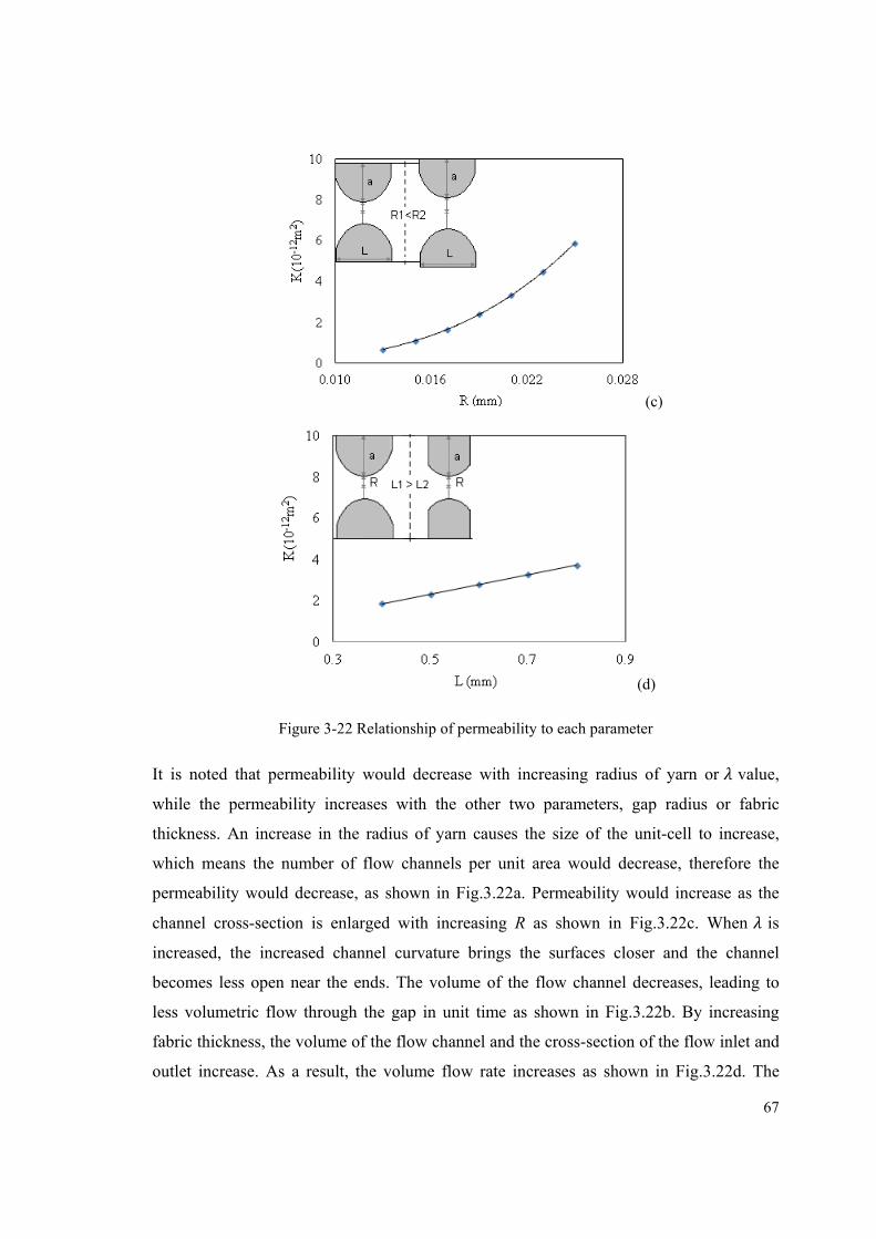
67

(c)

(d)

Figure 3-22 Relationship of permeability to each parameter

It is noted that permeability would decrease with increasing radius of yarn or value,

while the permeability increases with the other two parameters, gap radius or fabric

thickness. An increase in the radius of yarn causes the size of the unit-cell to increase,

which means the number of flow channels per unit area would decrease, therefore the

permeability would decrease, as shown in Fig.3.22a. Permeability would increase as the

channel cross-section is enlarged with increasing R as shown in Fig.3.22c. When is

increased, the increased channel curvature brings the surfaces closer and the channel

becomes less open near the ends. The volume of the flow channel decreases, leading to

less volumetric flow through the gap in unit time as shown in Fig.3.22b. By increasing

fabric thickness, the volume of the flow channel and the cross-section of the flow inlet and

outlet increase. As a result, the volume flow rate increases as shown in Fig.3.22d. The

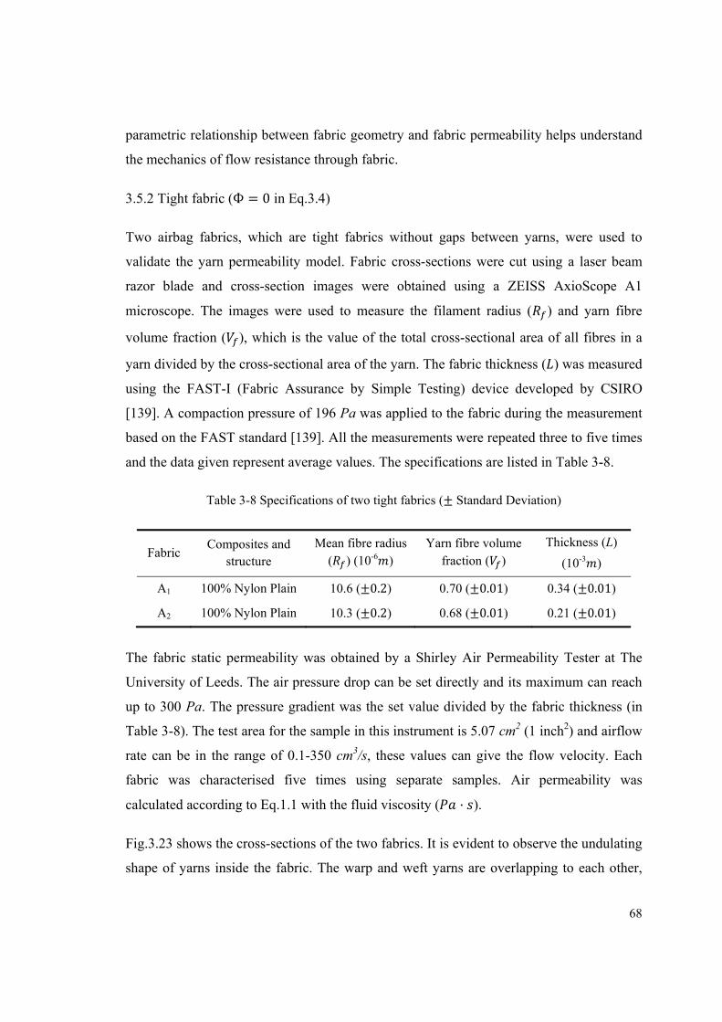
68

parametric relationship between fabric geometry and fabric permeability helps understand

the mechanics of flow resistance through fabric.

3.5.2 Tight fabric (Ф = 0 in Eq.3.4)

Two airbag fabrics, which are tight fabrics without gaps between yarns, were used to

validate the yarn permeability model. Fabric cross-sections were cut using a laser beam

razor blade and cross-section images were obtained using a ZEISS AxioScope A1

microscope. The images were used to measure the filament radius ( ) and yarn fibre

volume fraction ( ), which is the value of the total cross-sectional area of all fibres in a

yarn divided by the cross-sectional area of the yarn. The fabric thickness ( ) was measured

using the FAST-I (Fabric Assurance by Simple Testing) device developed by CSIRO

[139]. A compaction pressure of 196 Pa was applied to the fabric during the measurement

based on the FAST standard [139]. All the measurements were repeated three to five times

and the data given represent average values. The specifications are listed in Table 3-8.

Table 3-8 Specifications of two tight fabrics (± Standard Deviation)

Fabric Composites and

structure

Mean fibre radius ( ) (10-6 )

Yarn fibre volume fraction ( )

Thickness (L)

(10-3 )

A1 100% Nylon Plain 10.6 (±0.2) 0.70 (±0.01) 0.34 (±0.01)

A2 100% Nylon Plain 10.3 (±0.2) 0.68 (±0.01) 0.21 (±0.01)

The fabric static permeability was obtained by a Shirley Air Permeability Tester at The

University of Leeds. The air pressure drop can be set directly and its maximum can reach

up to 300 Pa. The pressure gradient was the set value divided by the fabric thickness (in

Table 3-8). The test area for the sample in this instrument is 5.07 cm2 (1 inch2) and airflow

rate can be in the range of 0.1-350 cm3/s, these values can give the flow velocity. Each

fabric was characterised five times using separate samples. Air permeability was

calculated according to Eq.1.1 with the fluid viscosity ( · ).

Fig.3.23 shows the cross-sections of the two fabrics. It is evident to observe the undulating

shape of yarns inside the fabric. The warp and weft yarns are overlapping to each other,

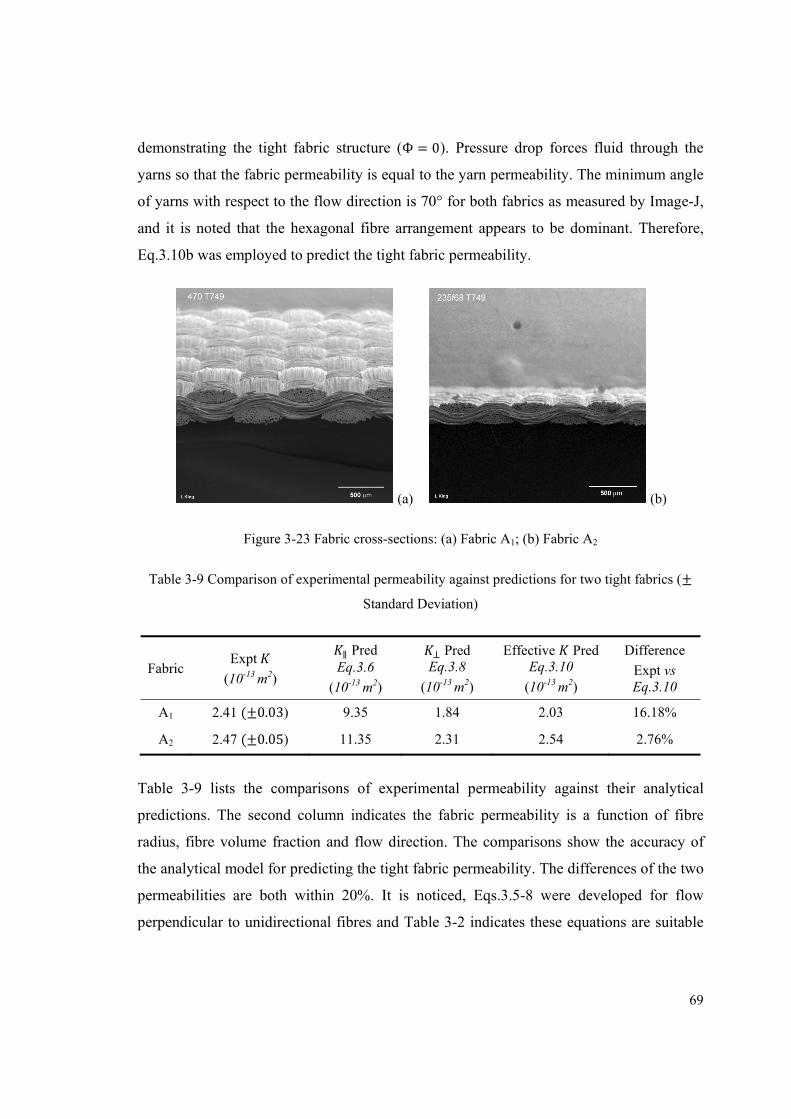
69

demonstrating the tight fabric structure (Ф = 0). Pressure drop forces fluid through the

yarns so that the fabric permeability is equal to the yarn permeability. The minimum angle

of yarns with respect to the flow direction is 70° for both fabrics as measured by Image-J,

and it is noted that the hexagonal fibre arrangement appears to be dominant. Therefore,

Eq.3.10b was employed to predict the tight fabric permeability.

(a) (b)

Figure 3-23 Fabric cross-sections: (a) Fabric A1; (b) Fabric A2

Table 3-9 Comparison of experimental permeability against predictions for two tight fabrics (±

Standard Deviation)

Fabric Expt

(10-13 m2)

∥ Pred Eq.3.6

(10-13 m2)

Pred Eq.3.8

(10-13 m2)

Effective Pred Eq.3.10

(10-13 m2)

Difference

Expt vs Eq.3.10

A1 2.41 (±0.03) 9.35 1.84 2.03 16.18%

A2 2.47 (±0.05) 11.35 2.31 2.54 2.76%

Table 3-9 lists the comparisons of experimental permeability against their analytical

predictions. The second column indicates the fabric permeability is a function of fibre

radius, fibre volume fraction and flow direction. The comparisons show the accuracy of

the analytical model for predicting the tight fabric permeability. The differences of the two

permeabilities are both within 20%. It is noticed, Eqs.3.5-8 were developed for flow

perpendicular to unidirectional fibres and Table 3-2 indicates these equations are suitable

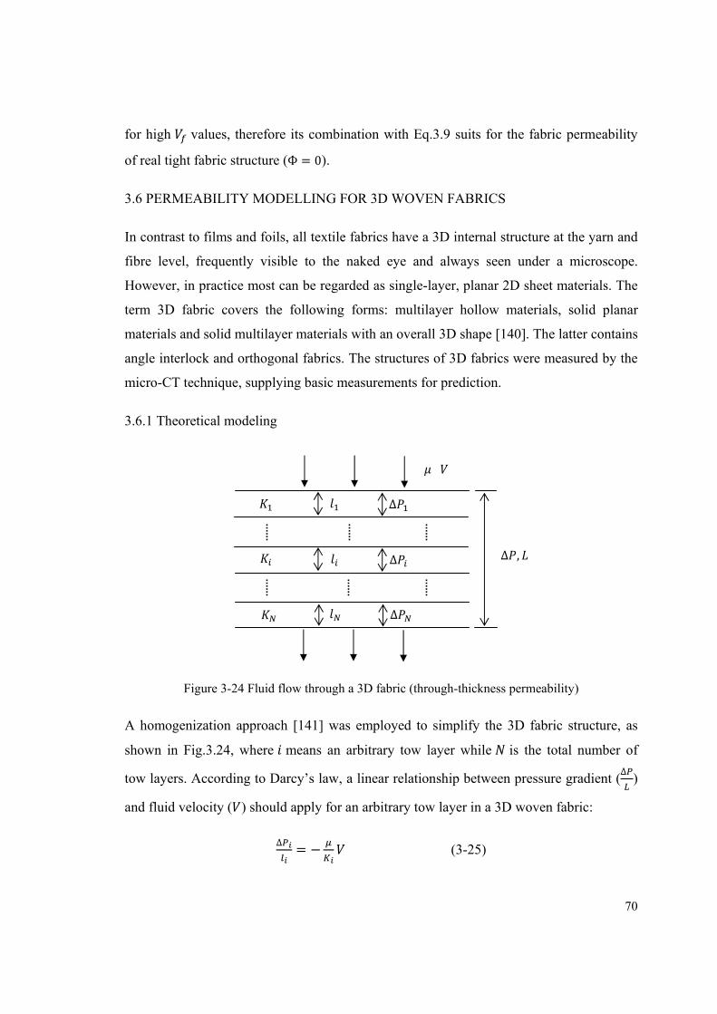
70

for high values, therefore its combination with Eq.3.9 suits for the fabric permeability

of real tight fabric structure (Ф = 0).

3.6 PERMEABILITY MODELLING FOR 3D WOVEN FABRICS

In contrast to films and foils, all textile fabrics have a 3D internal structure at the yarn and

fibre level, frequently visible to the naked eye and always seen under a microscope.

However, in practice most can be regarded as single-layer, planar 2D sheet materials. The

term 3D fabric covers the following forms: multilayer hollow materials, solid planar

materials and solid multilayer materials with an overall 3D shape [140]. The latter contains

angle interlock and orthogonal fabrics. The structures of 3D fabrics were measured by the

micro-CT technique, supplying basic measurements for prediction.

3.6.1 Theoretical modeling

Figure 3-24 Fluid flow through a 3D fabric (through-thickness permeability)

A homogenization approach [141] was employed to simplify the 3D fabric structure, as

shown in Fig.3.24, where means an arbitrary tow layer while is the total number of

tow layers. According to Darcy’s law, a linear relationship between pressure gradient (∆

)

and fluid velocity ( ) should apply for an arbitrary tow layer in a 3D woven fabric:

∆ = − (3-25)

∆ ,

∆∆∆

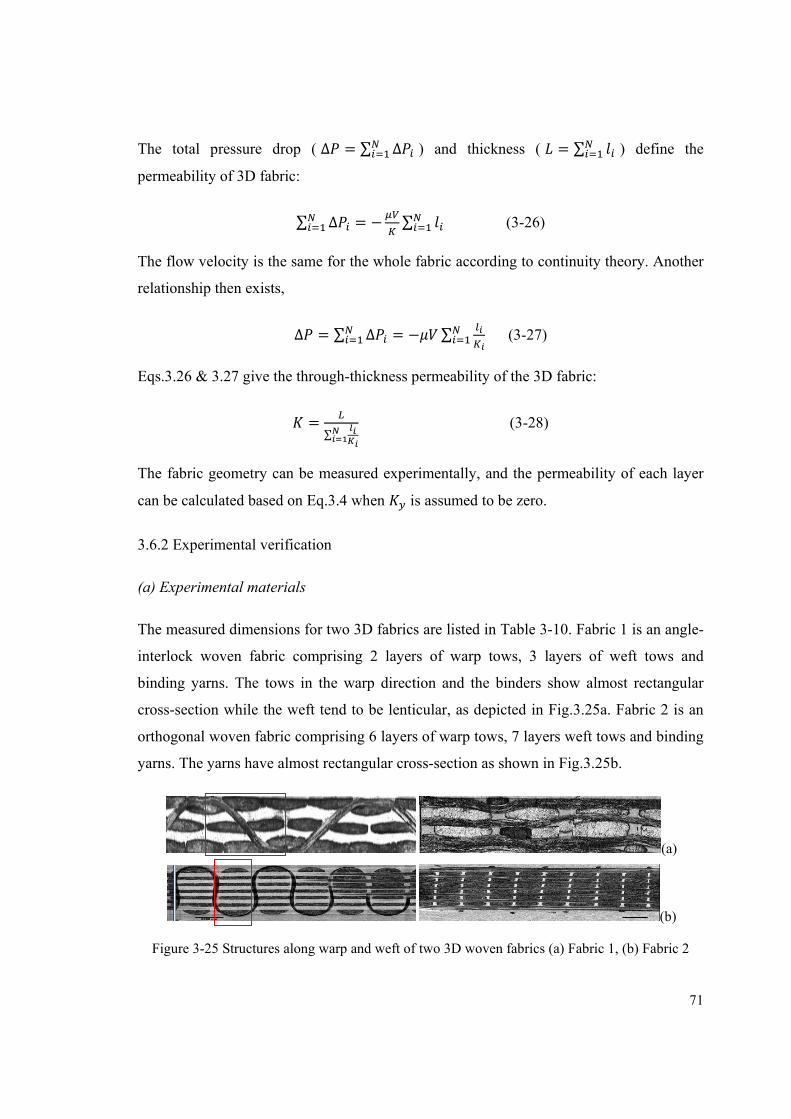
71

The total pressure drop ( ∆ = ∑ ∆ ) and thickness ( = ∑ ) define the

permeability of 3D fabric:

∑ ∆ = − ∑ (3-26)

The flow velocity is the same for the whole fabric according to continuity theory. Another

relationship then exists,

∆ = ∑ ∆ = − ∑ (3-27)

Eqs.3.26 & 3.27 give the through-thickness permeability of the 3D fabric:

= ∑ (3-28)

The fabric geometry can be measured experimentally, and the permeability of each layer

can be calculated based on Eq.3.4 when is assumed to be zero.

3.6.2 Experimental verification

(a) Experimental materials

The measured dimensions for two 3D fabrics are listed in Table 3-10. Fabric 1 is an angle-

interlock woven fabric comprising 2 layers of warp tows, 3 layers of weft tows and

binding yarns. The tows in the warp direction and the binders show almost rectangular

cross-section while the weft tend to be lenticular, as depicted in Fig.3.25a. Fabric 2 is an

orthogonal woven fabric comprising 6 layers of warp tows, 7 layers weft tows and binding

yarns. The yarns have almost rectangular cross-section as shown in Fig.3.25b.

(a)

(b)

Figure 3-25 Structures along warp and weft of two 3D woven fabrics (a) Fabric 1, (b) Fabric 2

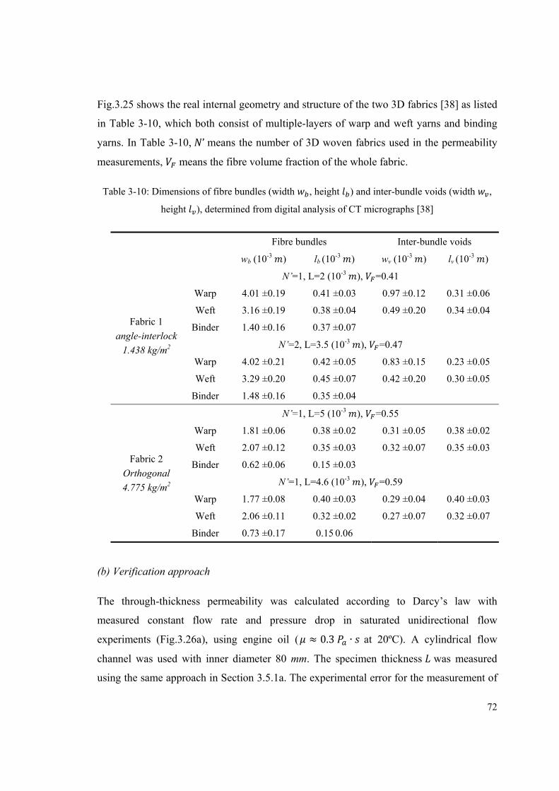
72

Fig.3.25 shows the real internal geometry and structure of the two 3D fabrics [38] as listed

in Table 3-10, which both consist of multiple-layers of warp and weft yarns and binding

yarns. In Table 3-10, ’ means the number of 3D woven fabrics used in the permeability

measurements, means the fibre volume fraction of the whole fabric.

Table 3-10: Dimensions of fibre bundles (width , height ) and inter-bundle voids (width ,

height ), determined from digital analysis of CT micrographs [38]

Fibre bundles Inter-bundle voids

wb (10-3 ) lb (10-3 ) wv (10-3 ) lv (10-3 )

Fabric 1

angle-interlock

1.438 kg/m2

N’=1, L=2 (10-3 ), =0.41

Warp 4.01 ±0.19 0.41 ±0.03 0.97 ±0.12 0.31 ±0.06

Weft 3.16 ±0.19 0.38 ±0.04 0.49 ±0.20 0.34 ±0.04

Binder 1.40 ±0.16 0.37 ±0.07

N’=2, L=3.5 (10-3 ), =0.47

Warp 4.02 ±0.21 0.42 ±0.05 0.83 ±0.15 0.23 ±0.05

Weft 3.29 ±0.20 0.45 ±0.07 0.42 ±0.20 0.30 ±0.05

Binder 1.48 ±0.16 0.35 ±0.04

Fabric 2

Orthogonal

4.775 kg/m2

N’=1, L=5 (10-3 ), =0.55

Warp 1.81 ±0.06 0.38 ±0.02 0.31 ±0.05 0.38 ±0.02

Weft 2.07 ±0.12 0.35 ±0.03 0.32 ±0.07 0.35 ±0.03

Binder 0.62 ±0.06 0.15 ±0.03

N’=1, L=4.6 (10-3 ), =0.59

Warp 1.77 ±0.08 0.40 ±0.03 0.29 ±0.04 0.40 ±0.03

Weft 2.06 ±0.11 0.32 ±0.02 0.27 ±0.07 0.32 ±0.07

Binder 0.73 ±0.17 0.15 0.06

(b) Verification approach

The through-thickness permeability was calculated according to Darcy’s law with

measured constant flow rate and pressure drop in saturated unidirectional flow

experiments (Fig.3.26a), using engine oil ( ≈ 0.3 ∙ at 20ºC). A cylindrical flow

channel was used with inner diameter 80 mm. The specimen thickness was measured

using the same approach in Section 3.5.1a. The experimental error for the measurement of

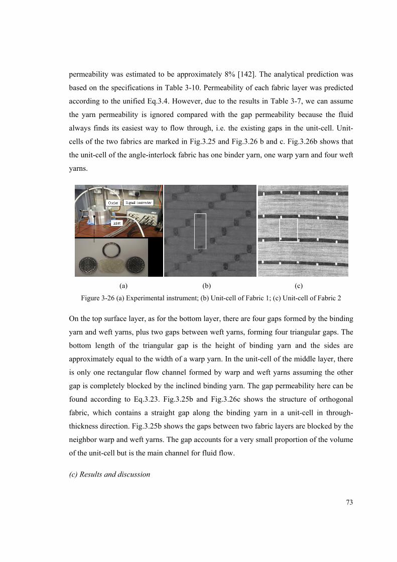
73

permeability was estimated to be approximately 8% [142]. The analytical prediction was

based on the specifications in Table 3-10. Permeability of each fabric layer was predicted

according to the unified Eq.3.4. However, due to the results in Table 3-7, we can assume

the yarn permeability is ignored compared with the gap permeability because the fluid

always finds its easiest way to flow through, i.e. the existing gaps in the unit-cell. Unit-

cells of the two fabrics are marked in Fig.3.25 and Fig.3.26 b and c. Fig.3.26b shows that

the unit-cell of the angle-interlock fabric has one binder yarn, one warp yarn and four weft

yarns.

(a) (b) (c)

Figure 3-26 (a) Experimental instrument; (b) Unit-cell of Fabric 1; (c) Unit-cell of Fabric 2

On the top surface layer, as for the bottom layer, there are four gaps formed by the binding

yarn and weft yarns, plus two gaps between weft yarns, forming four triangular gaps. The

bottom length of the triangular gap is the height of binding yarn and the sides are

approximately equal to the width of a warp yarn. In the unit-cell of the middle layer, there

is only one rectangular flow channel formed by warp and weft yarns assuming the other

gap is completely blocked by the inclined binding yarn. The gap permeability here can be

found according to Eq.3.23. Fig.3.25b and Fig.3.26c shows the structure of orthogonal

fabric, which contains a straight gap along the binding yarn in a unit-cell in through-

thickness direction. Fig.3.25b shows the gaps between two fabric layers are blocked by the

neighbor warp and weft yarns. The gap accounts for a very small proportion of the volume

of the unit-cell but is the main channel for fluid flow.

(c) Results and discussion

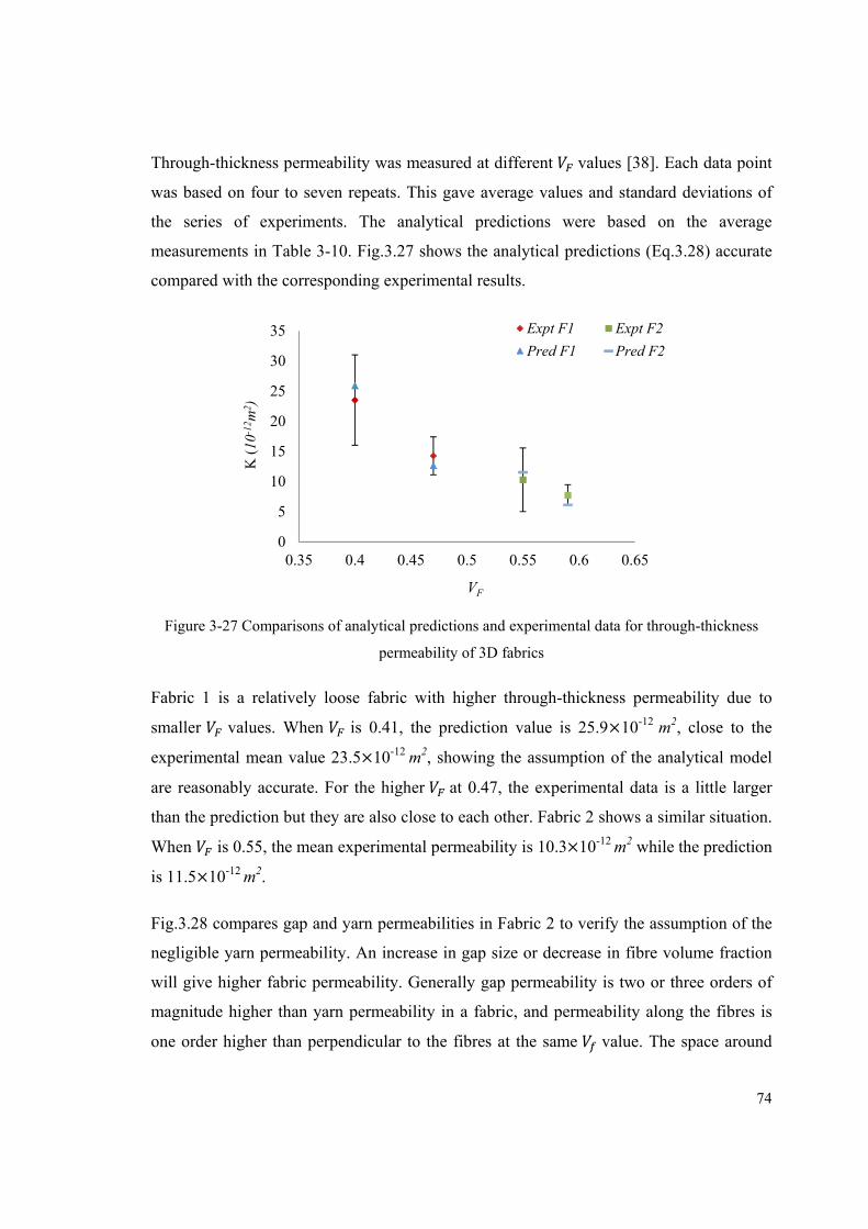
74

Through-thickness permeability was measured at different values [38]. Each data point

was based on four to seven repeats. This gave average values and standard deviations of

the series of experiments. The analytical predictions were based on the average

measurements in Table 3-10. Fig.3.27 shows the analytical predictions (Eq.3.28) accurate

compared with the corresponding experimental results.

Figure 3-27 Comparisons of analytical predictions and experimental data for through-thickness

permeability of 3D fabrics

Fabric 1 is a relatively loose fabric with higher through-thickness permeability due to

smaller values. When is 0.41, the prediction value is 25.9×10-12 m2, close to the

experimental mean value 23.5×10-12 m2, showing the assumption of the analytical model

are reasonably accurate. For the higher at 0.47, the experimental data is a little larger

than the prediction but they are also close to each other. Fabric 2 shows a similar situation.

When is 0.55, the mean experimental permeability is 10.3×10-12 m2 while the prediction

is 11.5×10-12 m2.

Fig.3.28 compares gap and yarn permeabilities in Fabric 2 to verify the assumption of the

negligible yarn permeability. An increase in gap size or decrease in fibre volume fraction

will give higher fabric permeability. Generally gap permeability is two or three orders of

magnitude higher than yarn permeability in a fabric, and permeability along the fibres is

one order higher than perpendicular to the fibres at the same value. The space around

0

5

10

15

20

25

30

35

0.35 0.4 0.45 0.5 0.55 0.6 0.65

K (

10-1

2 m2 )

VF

Expt F1 Expt F2

Pred F1 Pred F2

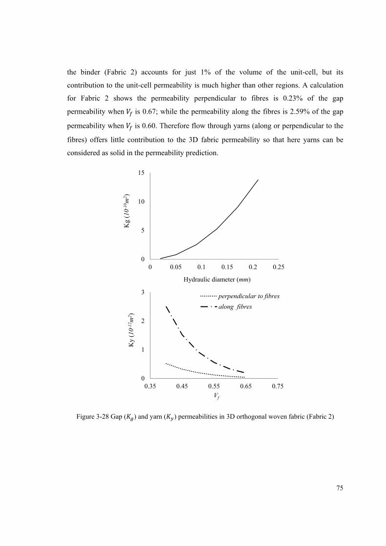
75

the binder (Fabric 2) accounts for just 1% of the volume of the unit-cell, but its

contribution to the unit-cell permeability is much higher than other regions. A calculation

for Fabric 2 shows the permeability perpendicular to fibres is 0.23% of the gap

permeability when is 0.67; while the permeability along the fibres is 2.59% of the gap

permeability when is 0.60. Therefore flow through yarns (along or perpendicular to the

fibres) offers little contribution to the 3D fabric permeability so that here yarns can be

considered as solid in the permeability prediction.

Figure 3-28 Gap ( ) and yarn ( ) permeabilities in 3D orthogonal woven fabric (Fabric 2)

0

5

10

15

0 0.05 0.1 0.15 0.2 0.25

Kg

(10-1

0 m2 )

Hydraulic diameter (mm)

0

1

2

3

0.35 0.45 0.55 0.65 0.75

Ky

(10-1

2 m2 )

Vf

perpendicular to fibres

along fibres

76

3.7 CONCLUSIONS

A unified static and through-thickness permeability model for one-layer of woven fabric

( ) was proposed. It is a function of yarn and gap permeabilities with respect to the fabric

areal porosity (Φ). The yarn and gap permeaiblities depend on the fabric geometric factors

completely, such as fibre radius and arrangement, yarn cross-section and fabric thickness.

When Φ = 0, i.e. yarns in a woven fabric touch each other or are even overlapping, fluid

has to flow through yarns completely. In this case, the fabric permeability equals the yarn

permeability. The Gebart model gives the permeability for fluid flow along and

perpendicular to unidirectional fibres. The Advani model considers fluid flow with an

angle in an anisotropic fabric. The yarn permeability model developed in this chapter

combines the Gebart model with the Advani model for predicting permeability of tight

fabrics. It is based on geometric factors including fibre radius and arrangement, fibre

volume fraction ( ) and the minimal angle (θ) of yarn path and flow direction. CFD

simulations showed the accuracy of perpendicular permeability prediction. However, for

flow along fibres, the simulation showed the prediction agreed well for large values but

poorly for small values. Two tight airbag fabrics were tested for their permeability. The

experimental results showed the analytical model can predict the tight fabric permeability

with a maximum error of 20%, indicating the yarn permeability model can be used for

tight fabrics with high values.

When Φ ≠ 0 , i.e. a loose woven fabric, a novel generic analytical model for gap

permeability was developed. The key feature in the model is that a parabolic function was

used within the Hagen-Poiseuille flow integration to capture the geometry of the flow

channel formed by interwoven yarns. Different channel shapes in various fabrics can be

represented by this with the parameter obtained from microscopic measurement. Five

gradual converging-diverging flow channels were simulated for flow behaviour in CFD.

After a sensitivity study, the calculated permeability is close to its analytical prediction.

For nine woven fabrics, the model gave good predictions compared with experimental data

for most fabrics. Predictions showed the gap permeability provide more than 89%

contribution to the loose fabric permeability. The Kulichenko model, where a straight flow

77

channel is assumed, gives over 70% error in permeability prediction. It is believed that the

inclusion of the geometry of the flow channel makes the gap permeaiblity model

significantly more accurate than existing models. A parametric study shows the influence

of four independent geometric variables relevant to fabric permeability.

A through-thickness permeability model for 3D woven fabric was derived based on the

permeability of each tow layer. The fabric structure was analyzed by the micro-CT

technique. Equations of flow through gaps were developed. Predictions and experimental

data were compared. The predictions showed good agreement with the experimental data,

proving the model to be reasonably accurate. A sensitivity study showed that the most

significant contribution to 3D fabric permeability was the gap between yarns.

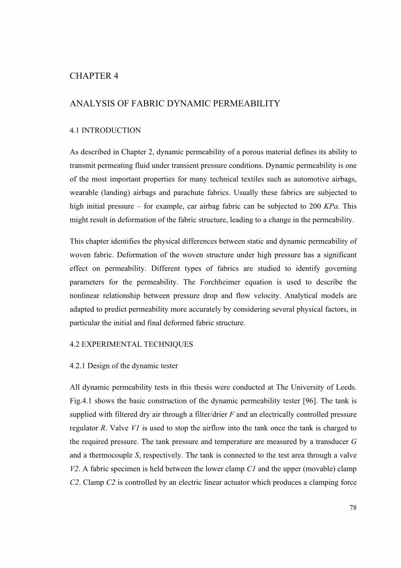
78

CHAPTER 4

ANALYSIS OF FABRIC DYNAMIC PERMEABILITY

4.1 INTRODUCTION

As described in Chapter 2, dynamic permeability of a porous material defines its ability to

transmit permeating fluid under transient pressure conditions. Dynamic permeability is one

of the most important properties for many technical textiles such as automotive airbags,

wearable (landing) airbags and parachute fabrics. Usually these fabrics are subjected to

high initial pressure – for example, car airbag fabric can be subjected to 200 KPa. This

might result in deformation of the fabric structure, leading to a change in the permeability.

This chapter identifies the physical differences between static and dynamic permeability of

woven fabric. Deformation of the woven structure under high pressure has a significant

effect on permeability. Different types of fabrics are studied to identify governing

parameters for the permeability. The Forchheimer equation is used to describe the

nonlinear relationship between pressure drop and flow velocity. Analytical models are

adapted to predict permeability more accurately by considering several physical factors, in

particular the initial and final deformed fabric structure.

4.2 EXPERIMENTAL TECHNIQUES

4.2.1 Design of the dynamic tester

All dynamic permeability tests in this thesis were conducted at The University of Leeds.

Fig.4.1 shows the basic construction of the dynamic permeability tester [96]. The tank is

supplied with filtered dry air through a filter/drier F and an electrically controlled pressure

regulator R. Valve V1 is used to stop the airflow into the tank once the tank is charged to

the required pressure. The tank pressure and temperature are measured by a transducer G

and a thermocouple S, respectively. The tank is connected to the test area through a valve

V2. A fabric specimen is held between the lower clamp C1 and the upper (movable) clamp

C2. Clamp C2 is controlled by an electric linear actuator which produces a clamping force

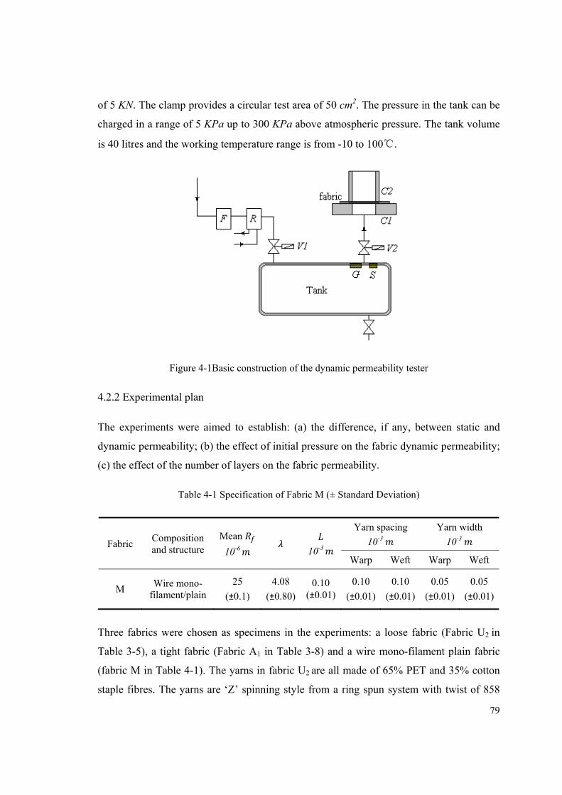
79

of 5 KN. The clamp provides a circular test area of 50 cm2. The pressure in the tank can be

charged in a range of 5 KPa up to 300 KPa above atmospheric pressure. The tank volume

is 40 litres and the working temperature range is from -10 to 100℃.

Figure 4-1Basic construction of the dynamic permeability tester

4.2.2 Experimental plan

The experiments were aimed to establish: (a) the difference, if any, between static and

dynamic permeability; (b) the effect of initial pressure on the fabric dynamic permeability;

(c) the effect of the number of layers on the fabric permeability.

Table 4-1 Specification of Fabric M (± Standard Deviation)

Fabric Composition and structure

Mean

10-6

10-3

Yarn spacing

10-3

Yarn width

10-3

Warp Weft Warp Weft

M Wire mono-

filament/plain 25

(±0.1)

4.08

(±0.80)0.10

(±0.01) 0.10

(±0.01)

0.10

(±0.01)

0.05

(±0.01)

0.05

(±0.01)

Three fabrics were chosen as specimens in the experiments: a loose fabric (Fabric U2 in

Table 3-5), a tight fabric (Fabric A1 in Table 3-8) and a wire mono-filament plain fabric

(fabric M in Table 4-1). The yarns in fabric U2 are all made of 65% PET and 35% cotton

staple fibres. The yarns are ‘Z’ spinning style from a ring spun system with twist of 858

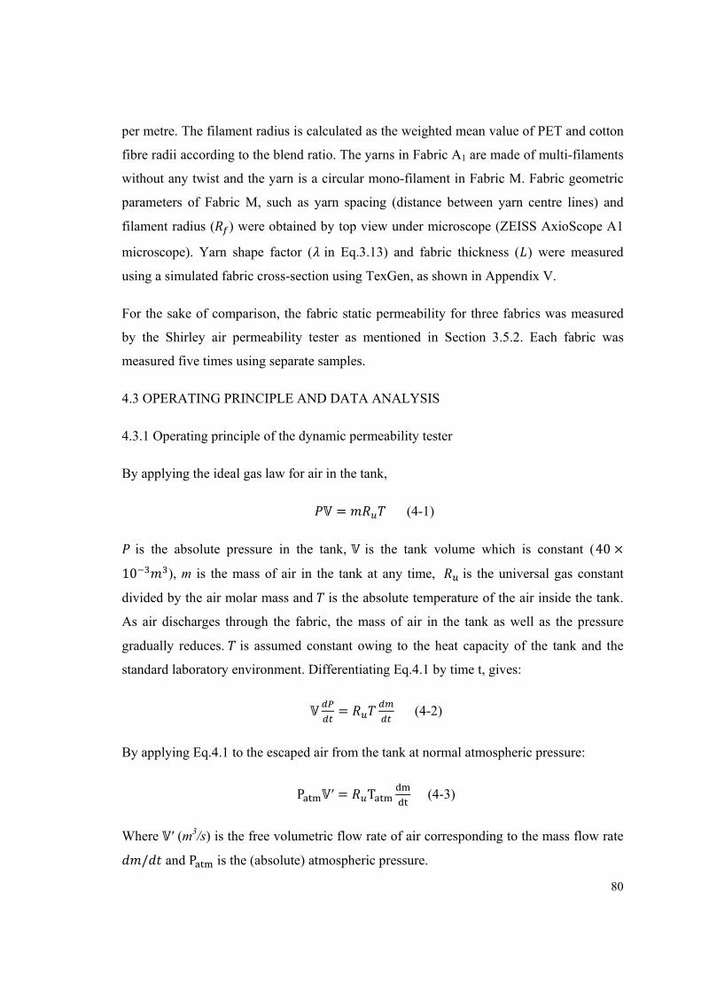
80

per metre. The filament radius is calculated as the weighted mean value of PET and cotton

fibre radii according to the blend ratio. The yarns in Fabric A1 are made of multi-filaments

without any twist and the yarn is a circular mono-filament in Fabric M. Fabric geometric

parameters of Fabric M, such as yarn spacing (distance between yarn centre lines) and

filament radius ( ) were obtained by top view under microscope (ZEISS AxioScope A1

microscope). Yarn shape factor ( in Eq.3.13) and fabric thickness ( ) were measured

using a simulated fabric cross-section using TexGen, as shown in Appendix V.

For the sake of comparison, the fabric static permeability for three fabrics was measured

by the Shirley air permeability tester as mentioned in Section 3.5.2. Each fabric was

measured five times using separate samples.

4.3 OPERATING PRINCIPLE AND DATA ANALYSIS

4.3.1 Operating principle of the dynamic permeability tester

By applying the ideal gas law for air in the tank,

= (4-1)

is the absolute pressure in the tank, is the tank volume which is constant (40 ×10 ), m is the mass of air in the tank at any time, is the universal gas constant

divided by the air molar mass and is the absolute temperature of the air inside the tank.

As air discharges through the fabric, the mass of air in the tank as well as the pressure

gradually reduces. is assumed constant owing to the heat capacity of the tank and the

standard laboratory environment. Differentiating Eq.4.1 by time t, gives:

= (4-2)

By applying Eq.4.1 to the escaped air from the tank at normal atmospheric pressure:

P ′ = T (4-3)

Where ′ (m3/s) is the free volumetric flow rate of air corresponding to the mass flow rate / and P is the (absolute) atmospheric pressure.

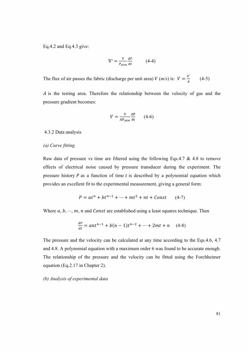
81

Eq.4.2 and Eq.4.3 give:

′ = (4-4)

The flux of air passes the fabric (discharge per unit area) (m/s) is: = ′ (4-5)

is the testing area. Therefore the relationship between the velocity of gas and the

pressure gradient becomes:

= (4-6)

4.3.2 Data analysis

(a) Curve fitting

Raw data of pressure vs time are filtered using the following Eqs.4.7 & 4.8 to remove

effects of electrical noise caused by pressure transducer during the experiment. The

pressure history as a function of time is described by a polynomial equation which

provides an excellent fit to the experimental measurement, giving a general form: = + +⋯+ + + (4-7)

Where , , ⋯, , and are established using a least squares technique. Then

= + ( − 1) +⋯+ 2 + (4-8)

The pressure and the velocity can be calculated at any time according to the Eqs.4.6, 4.7

and 4.8. A polynomial equation with a maximum order 6 was found to be accurate enough.

The relationship of the pressure and the velocity can be fitted using the Forchheimer

equation (Eq.2.17 in Chapter 2).

(b) Analysis of experimental data

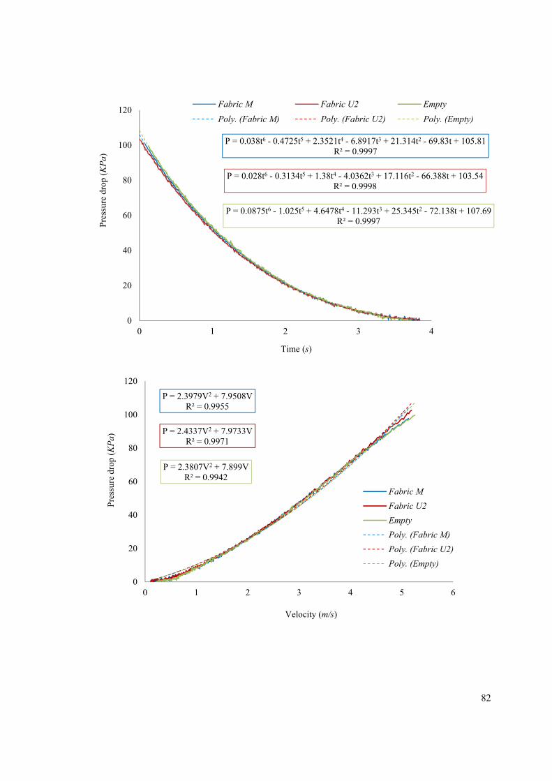
82

P = 0.038t6 - 0.4725t5 + 2.3521t4 - 6.8917t3 + 21.314t2 - 69.83t + 105.81R² = 0.9997

P = 0.028t6 - 0.3134t5 + 1.38t4 - 4.0362t3 + 17.116t2 - 66.388t + 103.54R² = 0.9998

P = 0.0875t6 - 1.025t5 + 4.6478t4 - 11.293t3 + 25.345t2 - 72.138t + 107.69R² = 0.9997

0

20

40

60

80

100

120

0 1 2 3 4

Pre

ssur

e dr

op (

KP

a)

Time (s)

Fabric M Fabric U2 Empty

Poly. (Fabric M) Poly. (Fabric U2) Poly. (Empty)

P = 2.3979V2 + 7.9508VR² = 0.9955

P = 2.4337V2 + 7.9733VR² = 0.9971

P = 2.3807V2 + 7.899VR² = 0.9942

0

20

40

60

80

100

120

0 1 2 3 4 5 6

Pre

ssur

e dr

op (

KP

a)

Velocity (m/s)

Fabric M

Fabric U2

Empty

Poly. (Fabric M)

Poly. (Fabric U2)

Poly. (Empty)

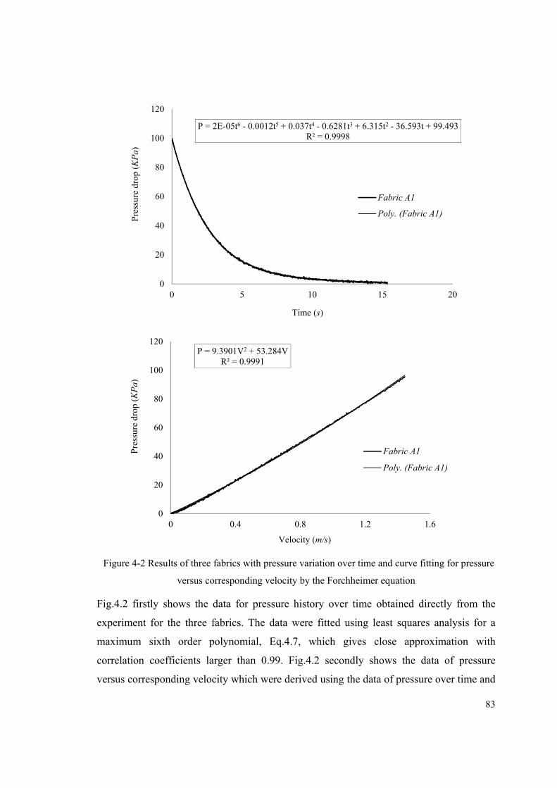
83

Figure 4-2 Results of three fabrics with pressure variation over time and curve fitting for pressure

versus corresponding velocity by the Forchheimer equation

Fig.4.2 firstly shows the data for pressure history over time obtained directly from the

experiment for the three fabrics. The data were fitted using least squares analysis for a

maximum sixth order polynomial, Eq.4.7, which gives close approximation with

correlation coefficients larger than 0.99. Fig.4.2 secondly shows the data of pressure

versus corresponding velocity which were derived using the data of pressure over time and

P = 2E-05t6 - 0.0012t5 + 0.037t4 - 0.6281t3 + 6.315t2 - 36.593t + 99.493R² = 0.9998

0

20

40

60

80

100

120

0 5 10 15 20

Pre

ssur

e dr

op (

KP

a)

Time (s)

Fabric A1

Poly. (Fabric A1)

P = 9.3901V2 + 53.284VR² = 0.9991

0

20

40

60

80

100

120

0 0.4 0.8 1.2 1.6

Pre

ssur

e dr

op (

KP

a)

Velocity (m/s)

Fabric A1

Poly. (Fabric A1)

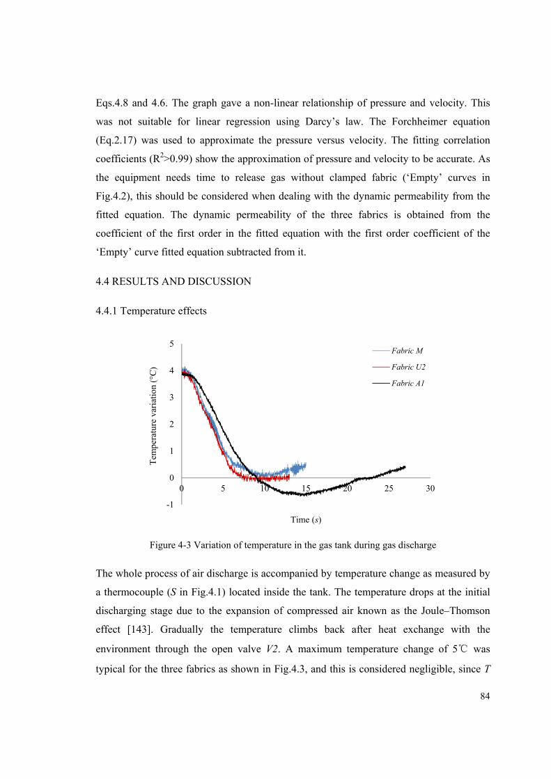
84

Eqs.4.8 and 4.6. The graph gave a non-linear relationship of pressure and velocity. This

was not suitable for linear regression using Darcy’s law. The Forchheimer equation

(Eq.2.17) was used to approximate the pressure versus velocity. The fitting correlation

coefficients (R2>0.99) show the approximation of pressure and velocity to be accurate. As

the equipment needs time to release gas without clamped fabric (‘Empty’ curves in

Fig.4.2), this should be considered when dealing with the dynamic permeability from the

fitted equation. The dynamic permeability of the three fabrics is obtained from the

coefficient of the first order in the fitted equation with the first order coefficient of the

‘Empty’ curve fitted equation subtracted from it.

4.4 RESULTS AND DISCUSSION

4.4.1 Temperature effects

Figure 4-3 Variation of temperature in the gas tank during gas discharge

The whole process of air discharge is accompanied by temperature change as measured by

a thermocouple (S in Fig.4.1) located inside the tank. The temperature drops at the initial

discharging stage due to the expansion of compressed air known as the Joule–Thomson

effect [143]. Gradually the temperature climbs back after heat exchange with the

environment through the open valve V2. A maximum temperature change of 5℃ was

typical for the three fabrics as shown in Fig.4.3, and this is considered negligible, since T

-1

0

1

2

3

4

5

0 5 10 15 20 25 30

Tem

pera

ture

var

iatio

n (°

C)

Time (s)

Fabric M

Fabric U2

Fabric A1

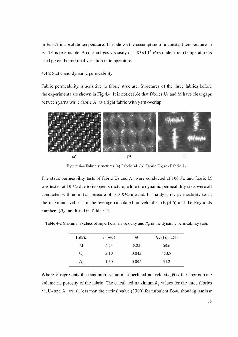
85

in Eq.4.2 is absolute temperature. This shows the assumption of a constant temperature in

Eq.4.4 is reasonable. A constant gas viscosity of 1.83×10-5 Pa·s under room temperature is

used given the minimal variation in temperature.

4.4.2 Static and dynamic permeability

Fabric permeability is sensitive to fabric structure. Structures of the three fabrics before

the experiments are shown in Fig.4.4. It is noticeable that fabrics U2 and M have clear gaps

between yarns while fabric A1 is a tight fabric with yarn overlap.

Figure 4-4 Fabric structures (a) Fabric M; (b) Fabric U2; (c) Fabric A1

The static permeability tests of fabric U2 and A1 were conducted at 100 Pa and fabric M

was tested at 10 Pa due to its open structure, while the dynamic permeability tests were all

conducted with an initial pressure of 100 KPa around. In the dynamic permeability tests,

the maximum values for the average calculated air velocities (Eq.4.6) and the Reynolds

numbers ( ) are listed in Table 4-2.

Table 4-2 Maximum values of superficial air velocity and in the dynamic permeability tests

Fabric V (m/s) ∅ (Eq.3.24)

M 5.23 0.25 68.6

U2 5.19 0.045 453.8

A1 1.30 0.005 34.2

Where V represents the maximum value of superficial air velocity, ∅ is the approximate

volumetric porosity of the fabric. The calculated maximum values for the three fabrics

M, U2 and A1 are all less than the critical value (2300) for turbulent flow, showing laminar

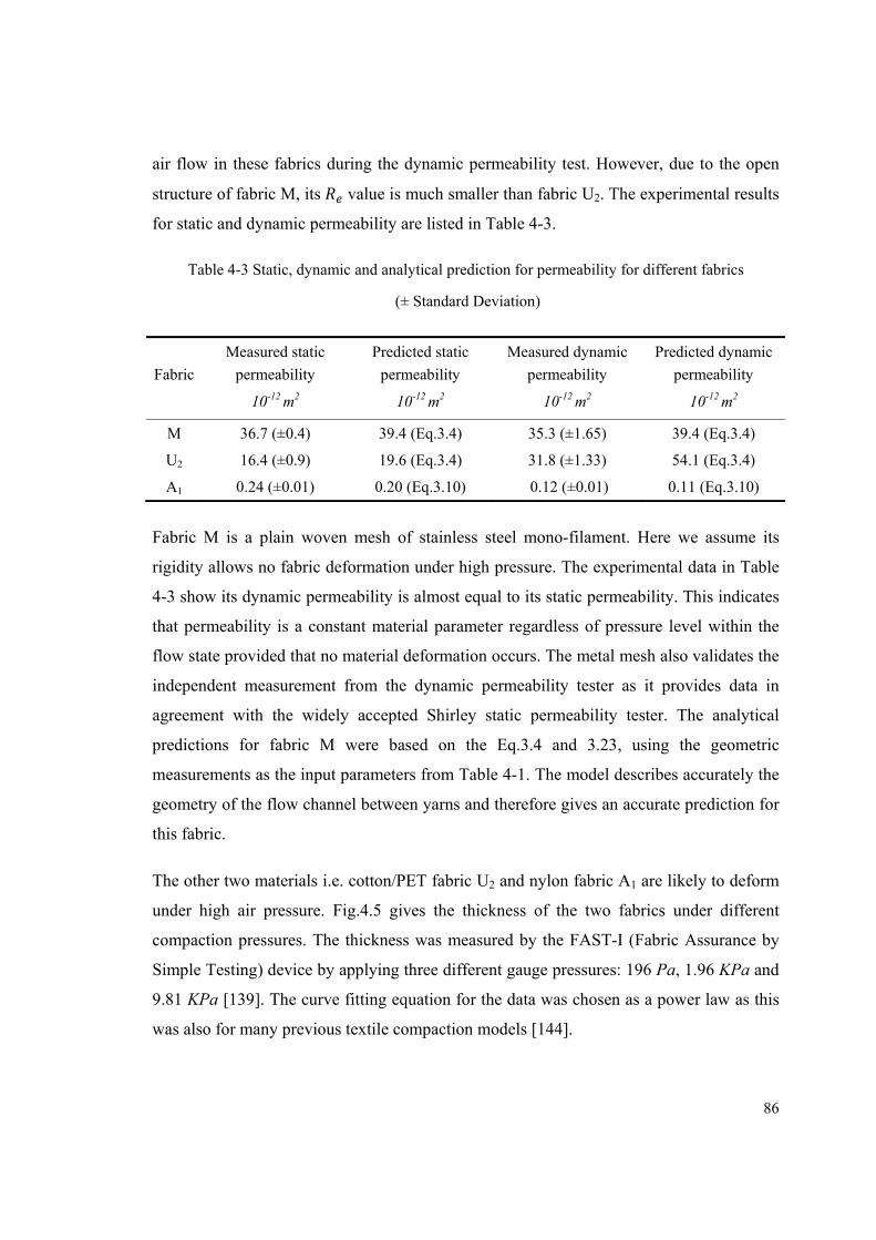
86

air flow in these fabrics during the dynamic permeability test. However, due to the open

structure of fabric M, its value is much smaller than fabric U2. The experimental results

for static and dynamic permeability are listed in Table 4-3.

Table 4-3 Static, dynamic and analytical prediction for permeability for different fabrics

(± Standard Deviation)

Fabric

Measured static

permeability

10-12 m2

Predicted static

permeability

10-12 m2

Measured dynamic

permeability

10-12 m2

Predicted dynamic

permeability

10-12 m2

M 36.7 (±0.4) 39.4 (Eq.3.4) 35.3 (±1.65) 39.4 (Eq.3.4)

U2 16.4 (±0.9) 19.6 (Eq.3.4) 31.8 (±1.33) 54.1 (Eq.3.4)

A1 0.24 (±0.01) 0.20 (Eq.3.10) 0.12 (±0.01) 0.11 (Eq.3.10)

Fabric M is a plain woven mesh of stainless steel mono-filament. Here we assume its

rigidity allows no fabric deformation under high pressure. The experimental data in Table

4-3 show its dynamic permeability is almost equal to its static permeability. This indicates

that permeability is a constant material parameter regardless of pressure level within the

flow state provided that no material deformation occurs. The metal mesh also validates the

independent measurement from the dynamic permeability tester as it provides data in

agreement with the widely accepted Shirley static permeability tester. The analytical

predictions for fabric M were based on the Eq.3.4 and 3.23, using the geometric

measurements as the input parameters from Table 4-1. The model describes accurately the

geometry of the flow channel between yarns and therefore gives an accurate prediction for

this fabric.

The other two materials i.e. cotton/PET fabric U2 and nylon fabric A1 are likely to deform

under high air pressure. Fig.4.5 gives the thickness of the two fabrics under different

compaction pressures. The thickness was measured by the FAST-I (Fabric Assurance by

Simple Testing) device by applying three different gauge pressures: 196 Pa, 1.96 KPa and

9.81 KPa [139]. The curve fitting equation for the data was chosen as a power law as this

was also for many previous textile compaction models [144].

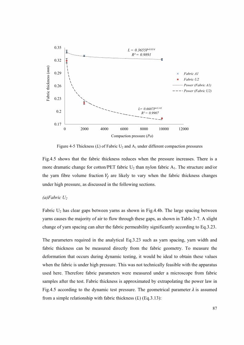
87

Figure 4-5 Thickness ( ) of Fabric U2 and A1 under different compaction pressures

Fig.4.5 shows that the fabric thickness reduces when the pressure increases. There is a

more dramatic change for cotton/PET fabric U2 than nylon fabric A1. The structure and/or

the yarn fibre volume fraction are likely to vary when the fabric thickness changes

under high pressure, as discussed in the following sections.

(a)Fabric U2

Fabric U2 has clear gaps between yarns as shown in Fig.4.4b. The large spacing between

yarns causes the majority of air to flow through these gaps, as shown in Table 3-7. A slight

change of yarn spacing can alter the fabric permeability significantly according to Eq.3.23.

The parameters required in the analytical Eq.3.23 such as yarn spacing, yarn width and

fabric thickness can be measured directly from the fabric geometry. To measure the

deformation that occurs during dynamic testing, it would be ideal to obtain these values

when the fabric is under high pressure. This was not technically feasible with the apparatus

used here. Therefore fabric parameters were measured under a microscope from fabric

samples after the test. Fabric thickness is approximated by extrapolating the power law in

Fig.4.5 according to the dynamic test pressure. The geometrical parameter is assumed

from a simple relationship with fabric thickness ( ) (Eq.3.13):

L = 0.3655P-0.014

R² = 0.9891

L= 0.6687P-0.143

R² = 0.9907

0.17

0.2

0.23

0.26

0.29

0.32

0.35

0 2000 4000 6000 8000 10000 12000

Fab

ric

thic

knes

s (m

m)

Compaction pressure (Pa)

Fabric A1

Fabric U2

Power (Fabric A1)

Power (Fabric U2)

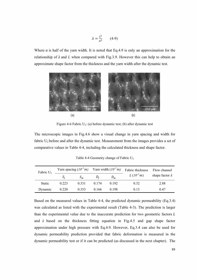
88

= (4-9)

Where is half of the yarn width. It is noted that Eq.4.9 is only an approximation for the

relationship of and L when compared with Fig.3.9. However this can help to obtain an

approximate shape factor from the thickness and the yarn width after the dynamic test.

Figure 4-6 Fabric U2: (a) before dynamic test; (b) after dynamic test

The microscopic images in Fig.4.6 show a visual change in yarn spacing and width for

fabric U2 before and after the dynamic test. Measurement from the images provides a set of

comparative values in Table 4-4, including the calculated thickness and shape factor.

Table 4-4 Geometry change of Fabric U2

Fabric U2 Yarn spacing (10-3 ) Yarn width (10-3 ) Fabric thickness

(10-3 )

Flow channel

shape factor

Static 0.223 0.331 0.174 0.192 0.32 2.88

Dynamic 0.220 0.353 0.166 0.198 0.13 0.47

Based on the measured values in Table 4-4, the predicted dynamic permeability (Eq.3.4)

was calculated as listed with the experimental result (Table 4-3). The prediction is larger

than the experimental value due to the inaccurate prediction for two geometric factors

and based on the thickness fitting equation in Fig.4.5 and gap shape factor

approximation under high pressure with Eq.4.9. However, Eq.3.4 can also be used for

dynamic permeability prediction provided that fabric deformation is measured in the

dynamic permeability test or if it can be predicted (as discussed in the next chapter). The

250 250

89

analytical model offers insight to explain the difference between dynamic and static

permeability. High pressure causes out-of-plane deformation, increasing the gap between

yarns while decreasing the fabric thickness and the shape factor of flow channel due to

the compaction at yarn crossovers. These changes explain why the fabric permeability is

higher for the dynamic permeability test.

(b) Fabric A1

Fabric A1 is a tight airbag fabric with overlapping yarns with no clear spacing as seen in

Fig.4.4c. Compared with the thickness reduction of 42% for fabric U2 as shown in Fig.4.5,

Fabric A1 has a thickness change of only 10% from compaction pressure 196 Pa to 9.81

KPa. This is due to the tight structure and high yarn for this fabric. The space between

fibres in yarns is the main flow channel for tight fabrics. Table 3-2 indicates that the

Gebart model (Eqs.3.5-8) is suitable for tight fibre bundle permeability prediction. For

fabric A1, the dynamic permeability decreases by almost half compared with the static

permeability as shown in Table 4-3. This trend is opposite to the fabric U2 which shows a

higher dynamic permeability. A similar experimental observation was found in the work of

Wang [94] where fabrics became less permeable under high pressure air impulse.

In the dynamic permeability test, the fabric was deflected and stretched by high pressure.

As dynamic permeability is lower than static permeability, this indicates that gaps did not

open between yarns in the dynamic test and the fabric became much tighter. The yarn fibre

volume fraction becomes larger under high pressure when the fabric thickness reduces

and fibre bundles are compacted together tightly. According to the hexagonal packing

theory, the maximum achievable fibre volume fraction ( ) is 0.907. The

corresponding pressure is 1.8×1010 Pa, which is the upper bound of pressure for the fitting

Eq.4.10. Assuming no other geometric deformation, yarn thickness reduction alone offers

an increased fibre volume fraction :

= (4-10)

Where is the measured original yarn fibre volume fraction from microscopic analysis of

un-deformed yarn cross section, is the original fabric thickness and is the thickness

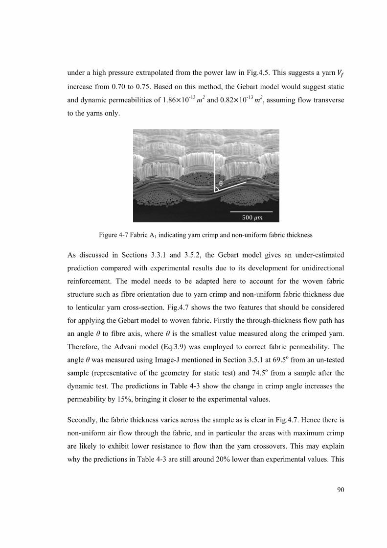
90

under a high pressure extrapolated from the power law in Fig.4.5. This suggests a yarn

increase from 0.70 to 0.75. Based on this method, the Gebart model would suggest static

and dynamic permeabilities of 1.86×10-13 m2 and 0.82×10-13 m2, assuming flow transverse

to the yarns only.

Figure 4-7 Fabric A1 indicating yarn crimp and non-uniform fabric thickness

As discussed in Sections 3.3.1 and 3.5.2, the Gebart model gives an under-estimated

prediction compared with experimental results due to its development for unidirectional

reinforcement. The model needs to be adapted here to account for the woven fabric

structure such as fibre orientation due to yarn crimp and non-uniform fabric thickness due

to lenticular yarn cross-section. Fig.4.7 shows the two features that should be considered

for applying the Gebart model to woven fabric. Firstly the through-thickness flow path has

an angle θ to fibre axis, where θ is the smallest value measured along the crimped yarn.

Therefore, the Advani model (Eq.3.9) was employed to correct fabric permeability. The

angle θ was measured using Image-J mentioned in Section 3.5.1 at 69.5o from an un-tested

sample (representative of the geometry for static test) and 74.5o from a sample after the

dynamic test. The predictions in Table 4-3 show the change in crimp angle increases the

permeability by 15%, bringing it closer to the experimental values.

Secondly, the fabric thickness varies across the sample as is clear in Fig.4.7. Hence there is

non-uniform air flow through the fabric, and in particular the areas with maximum crimp

are likely to exhibit lower resistance to flow than the yarn crossovers. This may explain

why the predictions in Table 4-3 are still around 20% lower than experimental values. This

θ

500

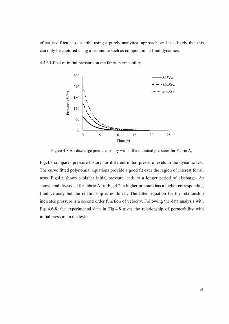
91

effect is difficult to describe using a purely analytical approach, and it is likely that this

can only be captured using a technique such as computational fluid dynamics.

4.4.3 Effect of initial pressure on the fabric permeability

Figure 4-8 Air discharge pressure history with different initial pressures for Fabric A1

Fig.4.8 compares pressure history for different initial pressure levels in the dynamic test.

The curve fitted polynomial equations provide a good fit over the region of interest for all

tests. Fig.4.8 shows a higher initial pressure leads to a longer period of discharge. As

shown and discussed for fabric A1 in Fig.4.2, a higher pressure has a higher corresponding

fluid velocity but the relationship is nonlinear. The fitted equation for the relationship

indicates pressure is a second order function of velocity. Following the data analysis with

Eqs.4.6-8, the experimental data in Fig.4.8 gives the relationship of permeability with

initial pressure in the test.

0

60

120

180

240

300

0 5 10 15 20 25

Pre

ssur

e (K

Pa)

Time (s)

80KPa

150KPa

250KPa

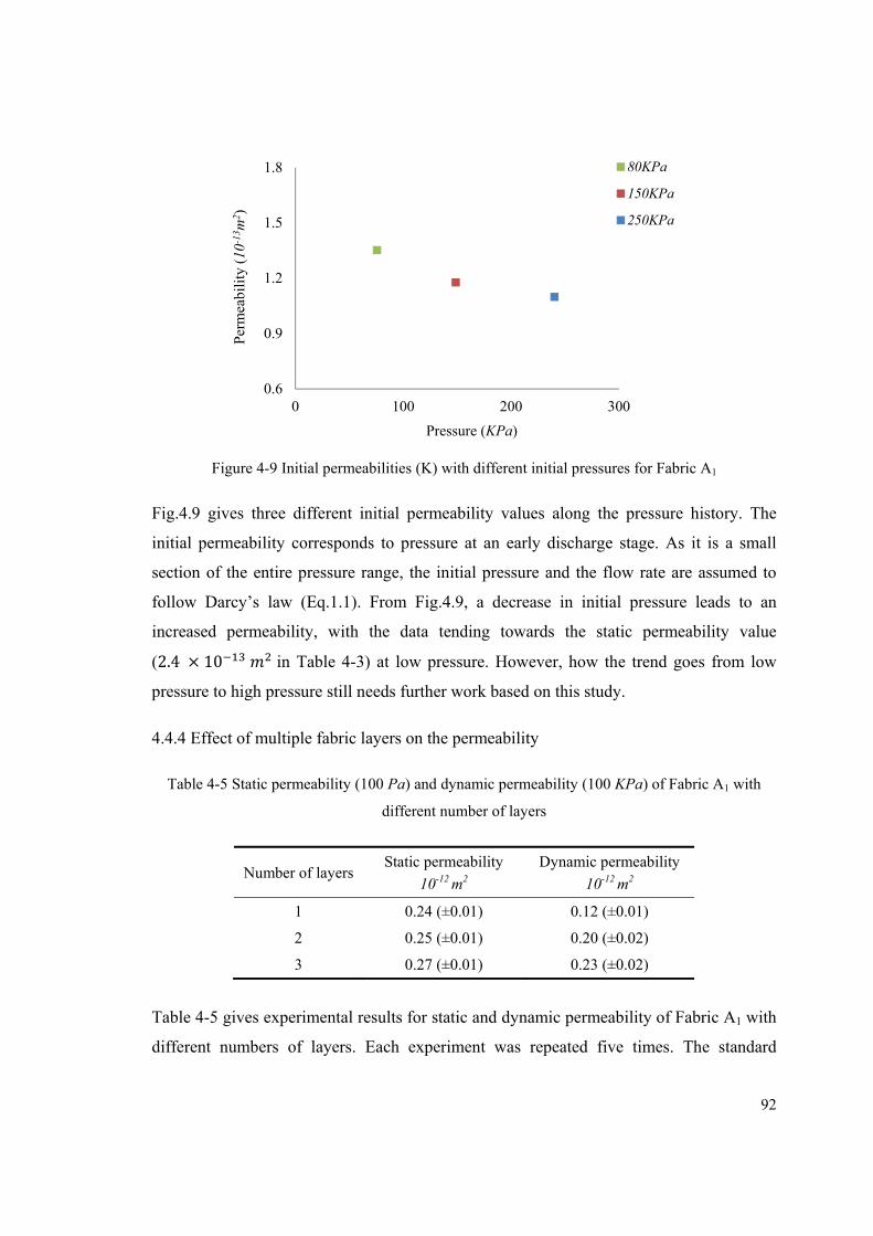
92

Figure 4-9 Initial permeabilities (K) with different initial pressures for Fabric A1

Fig.4.9 gives three different initial permeability values along the pressure history. The

initial permeability corresponds to pressure at an early discharge stage. As it is a small

section of the entire pressure range, the initial pressure and the flow rate are assumed to

follow Darcy’s law (Eq.1.1). From Fig.4.9, a decrease in initial pressure leads to an

increased permeability, with the data tending towards the static permeability value

(2.4 × 10 in Table 4-3) at low pressure. However, how the trend goes from low

pressure to high pressure still needs further work based on this study.

4.4.4 Effect of multiple fabric layers on the permeability

Table 4-5 Static permeability (100 Pa) and dynamic permeability (100 KPa) of Fabric A1 with

different number of layers

Number of layers Static permeability

10-12 m2

Dynamic permeability

10-12 m2

1 0.24 (±0.01) 0.12 (±0.01)

2 0.25 (±0.01) 0.20 (±0.02)

3 0.27 (±0.01) 0.23 (±0.02)

Table 4-5 gives experimental results for static and dynamic permeability of Fabric A1 with

different numbers of layers. Each experiment was repeated five times. The standard

0.6

0.9

1.2

1.5

1.8

0 100 200 300

Perm

eabi

lity

(10

-13 m

2 )

Pressure (KPa)

80KPa

150KPa

250KPa

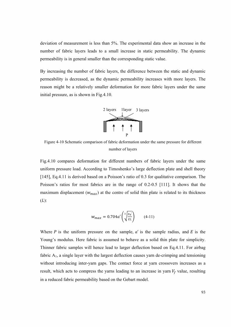
93

deviation of measurement is less than 5%. The experimental data show an increase in the

number of fabric layers leads to a small increase in static permeability. The dynamic

permeability is in general smaller than the corresponding static value.

By increasing the number of fabric layers, the difference between the static and dynamic

permeability is decreased, as the dynamic permeability increases with more layers. The

reason might be a relatively smaller deformation for more fabric layers under the same

initial pressure, as is shown in Fig.4.10.

Figure 4-10 Schematic comparison of fabric deformation under the same pressure for different

number of layers

Fig.4.10 compares deformation for different numbers of fabric layers under the same

uniform pressure load. According to Timoshenko’s large deflection plate and shell theory

[145], Eq.4.11 is derived based on a Poisson’s ratio of 0.3 for qualitative comparison. The

Poisson’s ratios for most fabrics are in the range of 0.2-0.5 [111]. It shows that the

maximum displacement ( ) at the centre of solid thin plate is related to its thickness

( ):

= 0.704 ′ ′3 (4-11)

Where is the uniform pressure on the sample, ′ is the sample radius, and is the

Young’s modulus. Here fabric is assumed to behave as a solid thin plate for simplicity.

Thinner fabric samples will hence lead to larger deflection based on Eq.4.11. For airbag

fabric A1, a single layer with the largest deflection causes yarn de-crimping and tensioning

without introducing inter-yarn gaps. The contact force at yarn crossovers increases as a

result, which acts to compress the yarns leading to an increase in yarn value, resulting

in a reduced fabric permeability based on the Gebart model.

P

2 layers 1layer 3 layers

94

4.5 CONCLUSIONS

Dynamic permeability is obtained by discharging air with high initial pressure through

woven fabrics. The transient pressure causes a fabric structural deformation. The

behaviour is different from the static permeability test applying a constant small pressure

drop. The Forchheimer equation, describing a nonlinear relationship between pressure and

velocity, is used to analyze the dynamic experimental data. The experimental data for the

metal mesh fabric show little difference between static and dynamic permeability, because

the fabric structure was not changed under high pressure. This also validates the dynamic

permeability test method compared with the widely accepted Shirley static permeability

test. Most fabrics are less rigid and are prone to deformation during the dynamic

permeability test. One example is a cotton/PET fabric with a loose structure, which is

easily deformed under pressure. The dynamic permeability for this fabric is much higher

than its static permeability. A trial analytical model shows that the increase in yarn spacing

due to fabric deflection leads to the higher permeability. In contrast, a tight fabric such as a

nylon airbag fabric had a lower dynamic permeability than its static value. The reason

might be the high pressure applied to this fabric results in a higher yarn fibre volume

fraction. Experiments also show that more fabric layers would have a larger dynamic

permeability for tight fabric. It is proposed that this is due to reduced deflection which in

turn causes less compaction at yarn crossovers and hence higher yarn permeability. The

next chapter will attempt to predict the deformation that occurs during dynamic testing and

to combine this with the analytical modelling approach to provide a fully predictive model

for through-thickness permeability.

95

CHAPTER 5

PERMEABILITY MODELLING OF DEFORMED TEXTILES UNDER

HIGH PRESSURE LOAD

5.1 INTRODUCTION

It is important to model out-of-plane fabric deformation under high pressure load, as the

alteration of fabric structure leads to a change in permeability as demonstrated in Chapter

4. Technical textiles, for application in airbags for instance, are usually subjected to a

normal pressure load. The load causes the fabric to deform, resulting in changes to

geometric parameters such as yarn fibre volume fraction and gap size. Therefore, it is

desirable to develop a predictive model of fabric deformation as a function of the load, as

well as to predict the corresponding permeability of the deformed fabric.

In the first part of this chapter, the energy method reviewed in Section 2.4.2 is employed to

analyze the fabric deformation. Polar coordinates are utilized to derive the equations for a

fully clamped circular fabric sheet. Expressions for describing the out-of-plane deflections

and for the in-plane stretching of the deformed fabric are developed by considering the

appropriate boundary conditions during deflection. Thereafter strain energy, bending

energy and work done are introduced to the total potential energy of the system, from

which the deflected shape is obtained by minimizing its total energy. The predictions for

the deformed fabric profile and its maximum displacement are validated with experimental

measurements.

In the second part, based on the fabric deformation model, the effects of pressure load are

taken into account on the geometric parameters for permeability prediction. Two fabrics

(one tight and one loose fabric) are employed to make the verifications. Comparisons of

experimental results with analytical predictions are performed at the end of the chapter. A

sensitivity study for each geometric factor helps understanding of pressure load on fabric

permeability.

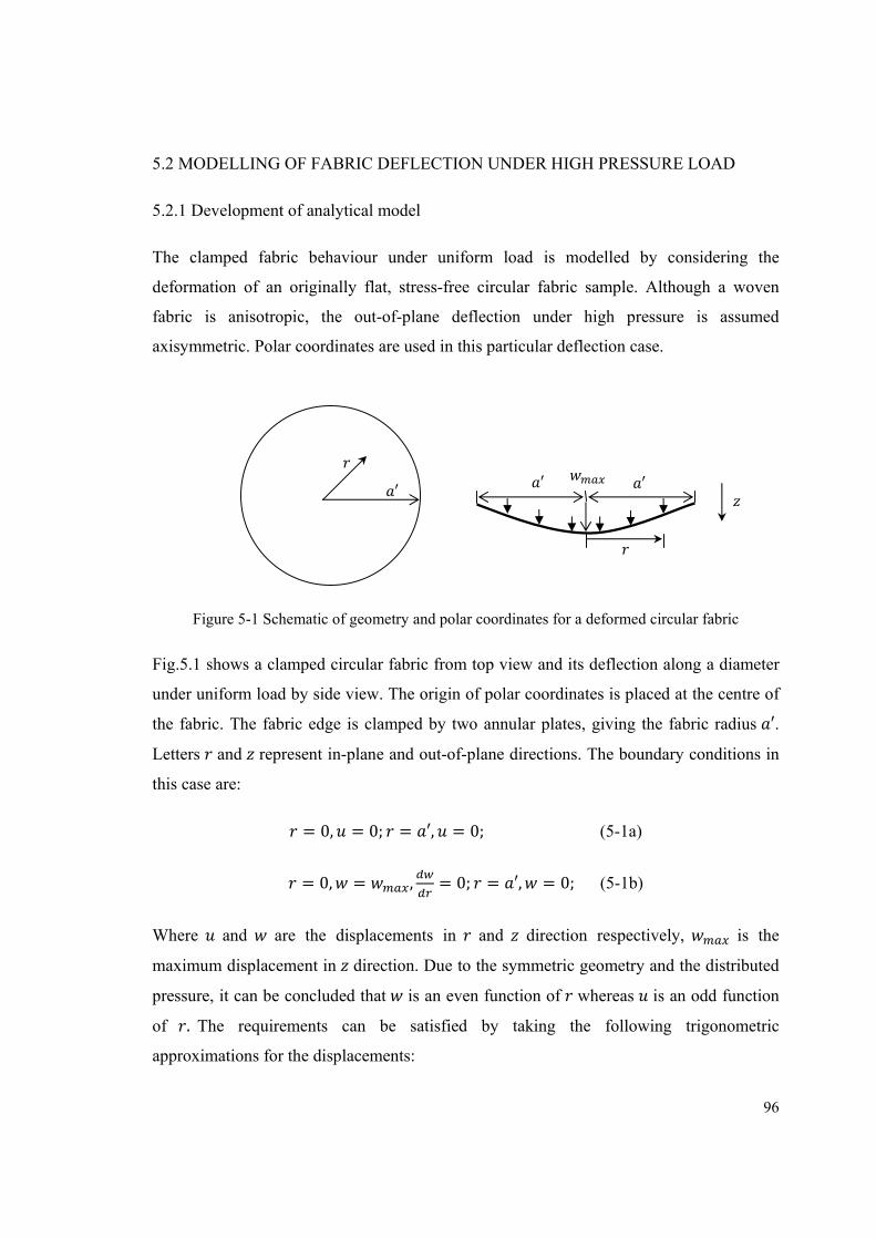
96

5.2 MODELLING OF FABRIC DEFLECTION UNDER HIGH PRESSURE LOAD

5.2.1 Development of analytical model

The clamped fabric behaviour under uniform load is modelled by considering the

deformation of an originally flat, stress-free circular fabric sample. Although a woven

fabric is anisotropic, the out-of-plane deflection under high pressure is assumed

axisymmetric. Polar coordinates are used in this particular deflection case.

Figure 5-1 Schematic of geometry and polar coordinates for a deformed circular fabric

Fig.5.1 shows a clamped circular fabric from top view and its deflection along a diameter

under uniform load by side view. The origin of polar coordinates is placed at the centre of

the fabric. The fabric edge is clamped by two annular plates, giving the fabric radius ′. Letters and represent in-plane and out-of-plane directions. The boundary conditions in

this case are: = 0, = 0; = ′, = 0; (5-1a)

= 0, = , = 0; = ′, = 0; (5-1b)

Where and are the displacements in and direction respectively, is the

maximum displacement in direction. Due to the symmetric geometry and the distributed

pressure, it can be concluded that is an even function of whereas is an odd function

of . The requirements can be satisfied by taking the following trigonometric

approximations for the displacements:

′ ′′

97

= ∗ sin( ) (5-2a) = cos( ) (5-2b)

Where is an arbitrary constant. Note that the shape of Eqs.5.2 is different with the

reviewed approximation Eq.2.30 which exhibits less gradual deflection near the edge of

clamped area as will be discussed in Section 5.2.3b. The problem of determining the fabric

deflection reduces to derivation of the coefficients and in Eqs.5.2. The coefficients

can be determined by the principle of virtual displacements. The energy method mentioned

in Section 2.4.2 is employed. Three types of energy occur during deflection: bending

energy , membrane strain energy and work done . Firstly , which is important

for a rigid and continuous sheet, herein has little contribution to the total deformation

energy due to the flexible and discontinuous fabric structure. The expression in polar

coordinate is transferred from Eq.2.33 as follows:

= ∬ { + + − 2(1 − ) + + 2(1 − ) −} (5-3)

The Eq.5.3 can be reduced to a simple form due to the axisymmetric bending in this case:

= D { + − ( ) } (5-4)

Where D is the fabric flexural rigidity, which does not equal ( ) for fabric [120] ( is

the Young’s modulus of fabric, is the fabric thickness and v is the Poisson’s ratio of

fabric) because the filaments in fabric bend relative to their own neutral axis rather than

that of the fabric.

Membrane strain energy plays a pivotal role in fabric deformation. It consists of stretching

and shearing energy during the fabric deflection. A common expression is rewritten from

Eq.2.32 in polar coordinates:

= { + + 2 } (5-5)

98

Where , are the radial and tangential normal strains. The relationships of strains and

displacements are:

= + ( ) (5-6a) = (5-6b)

By substitution of the values of the strains from Eqs.5.6 into the preceding equation, the

expression of is obtained in the form:

= { + + + + + } (5-7)

Where the component expression ( +′) represents shearing

energy and the rest is tensile energy. Eq.5.7 is a simplified expression due to the thin

axisymmetrically loaded circular shape.

As the circular fabric is deflected in the out-of–plane direction, the work done caused

by the pressure load can be obtained by integrating across the area of the fabric based

on Eq.2.34:

= 2 (5-8)

Therefore the potential energy function ( Π) for the system contains the bending energy,

the membrane strain energy and the work done:

Π = + + (5-9)

In which, relates bending strain energy, which concerns out-of-plane deformation;

links membrane strain energy to the fabric Young’s modulus, which concerns in-plane

deformation; denotes the work done by the uniformly distributed pressure load.

With the assumed deflected fabric shape (Eqs.5.2), the first order and second order of

derivatives with respect to the fabric radius ( ) are:

99

= cos (5-10a)

= − sin (5-10b)

= − cos (5-10c)

By substituting Eq.5.10 into Eq.5.4 and Eq.5.7 then integrating over the clamped fabric,

and integrating Eq. 5.8, the results are:

= ( + ln ) (5-11a)

= ( − − + + + + ln 2)

(5-11b) = 4(1 − ) (5-11c)

In Eq.5.11b, the condition = 0 that can make a minimum leads to:

= + / + ln 2 (5-12)

Inserting Eq.5.12 and Eqs.5.11 into Eq.5.9 with a numerical calculation:

Π = . . + ( . . ) − 1.4535 (5-13)

Then, application of the minimizing condition, Π = 0, yields approximate expressions

for the maximum deflection and out-of-plane displacement in the forms:

≅ ∙ . ∙ . . (5-14a)

= ∙ . ∙ . . ∙ cos( ) (5-14b)

It is noted that, here fabric has been viewed as a very thin ‘plate’ as the maximum

deflection is much greater than the fabric thickness. In this condition, the resistance

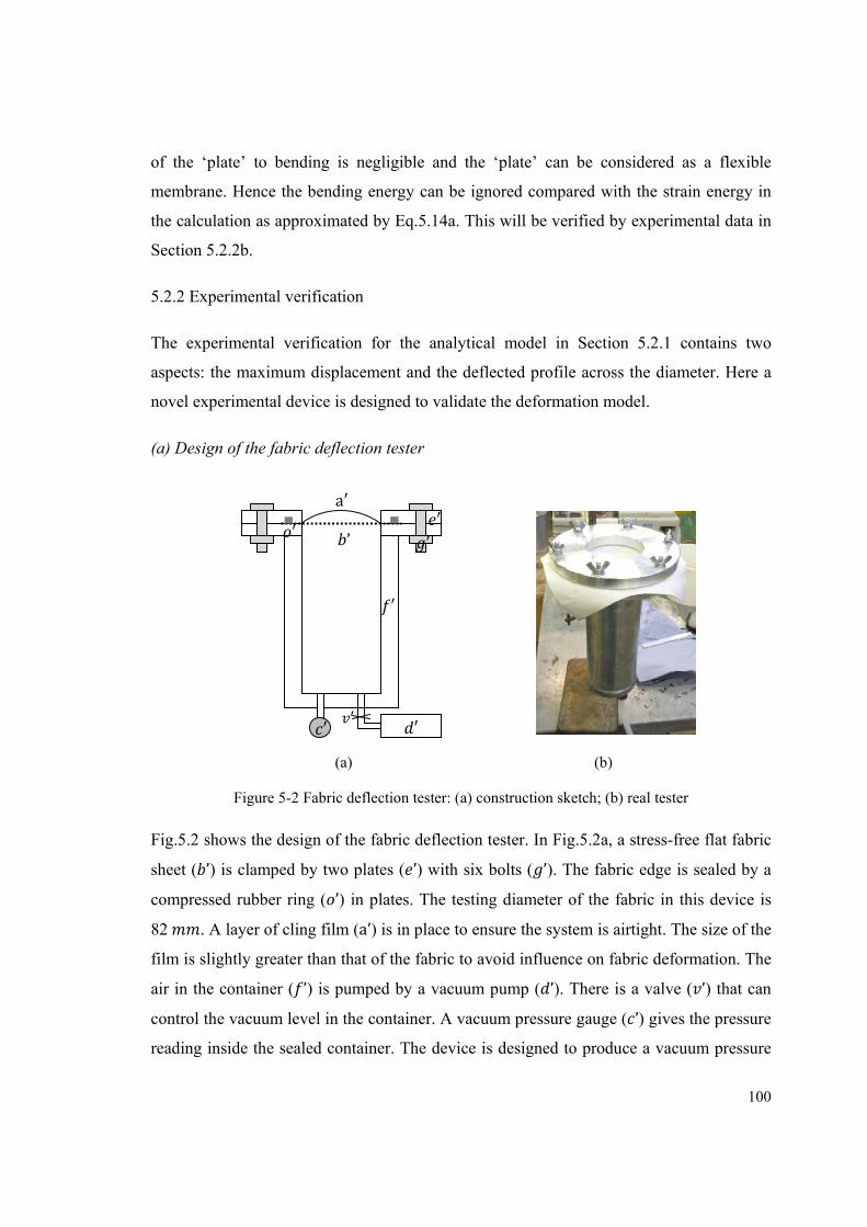
100

of the ‘plate’ to bending is negligible and the ‘plate’ can be considered as a flexible

membrane. Hence the bending energy can be ignored compared with the strain energy in

the calculation as approximated by Eq.5.14a. This will be verified by experimental data in

Section 5.2.2b.

5.2.2 Experimental verification

The experimental verification for the analytical model in Section 5.2.1 contains two

aspects: the maximum displacement and the deflected profile across the diameter. Here a

novel experimental device is designed to validate the deformation model.

(a) Design of the fabric deflection tester

(a) (b)

Figure 5-2 Fabric deflection tester: (a) construction sketch; (b) real tester

Fig.5.2 shows the design of the fabric deflection tester. In Fig.5.2a, a stress-free flat fabric

sheet ( ’) is clamped by two plates ( ’) with six bolts ( ’). The fabric edge is sealed by a

compressed rubber ring ( ’) in plates. The testing diameter of the fabric in this device is

82 . A layer of cling film (a’) is in place to ensure the system is airtight. The size of the

film is slightly greater than that of the fabric to avoid influence on fabric deformation. The

air in the container ( ’) is pumped by a vacuum pump ( ’). There is a valve ( ’) that can

control the vacuum level in the container. A vacuum pressure gauge ( ’) gives the pressure

reading inside the sealed container. The device is designed to produce a vacuum pressure

ℎ

′

a′ ’

′ ′

′′

′′

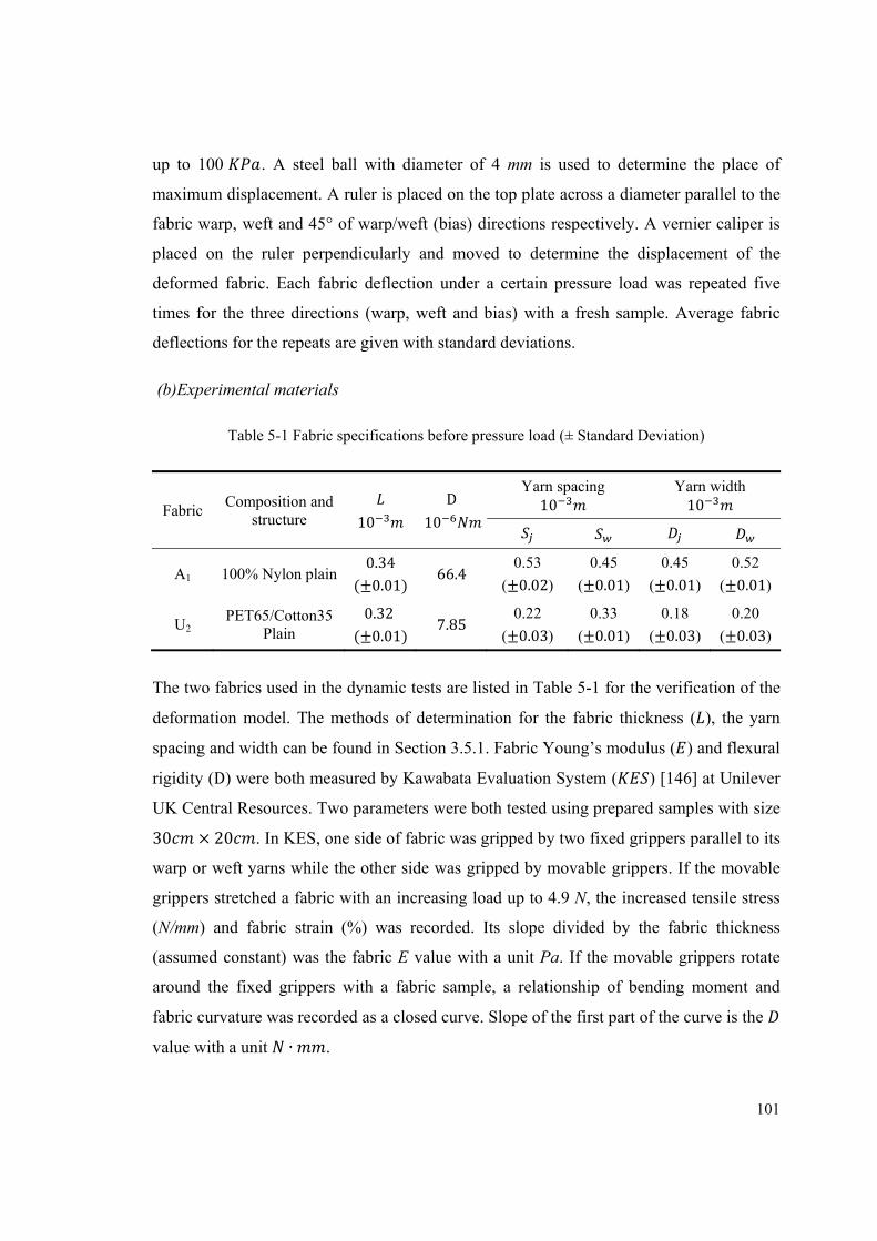
101

up to 100 . A steel ball with diameter of 4 mm is used to determine the place of

maximum displacement. A ruler is placed on the top plate across a diameter parallel to the

fabric warp, weft and 45° of warp/weft (bias) directions respectively. A vernier caliper is

placed on the ruler perpendicularly and moved to determine the displacement of the

deformed fabric. Each fabric deflection under a certain pressure load was repeated five

times for the three directions (warp, weft and bias) with a fresh sample. Average fabric

deflections for the repeats are given with standard deviations.

(b)Experimental materials

Table 5-1 Fabric specifications before pressure load (± Standard Deviation)

Fabric Composition and

structure 10

D10 Yarn spacing 10 Yarn width 10

A1 100% Nylon plain 0.34 (±0.01) 66.4

0.53

(±0.02)

0.45

(±0.01)

0.45

(±0.01)

0.52

(±0.01)

U2 PET65/Cotton35

Plain 0.32 (±0.01) 7.85

0.22

(±0.03)

0.33

(±0.01)

0.18

(±0.03)

0.20

(±0.03)

The two fabrics used in the dynamic tests are listed in Table 5-1 for the verification of the

deformation model. The methods of determination for the fabric thickness ( ), the yarn

spacing and width can be found in Section 3.5.1. Fabric Young’s modulus ( ) and flexural

rigidity (D) were both measured by Kawabata Evaluation System ( ) [146] at Unilever

UK Central Resources. Two parameters were both tested using prepared samples with size 30 × 20 . In KES, one side of fabric was gripped by two fixed grippers parallel to its

warp or weft yarns while the other side was gripped by movable grippers. If the movable

grippers stretched a fabric with an increasing load up to 4.9 N, the increased tensile stress

(N/mm) and fabric strain (%) was recorded. Its slope divided by the fabric thickness

(assumed constant) was the fabric E value with a unit Pa. If the movable grippers rotate

around the fixed grippers with a fabric sample, a relationship of bending moment and

fabric curvature was recorded as a closed curve. Slope of the first part of the curve is the

value with a unit ∙ .

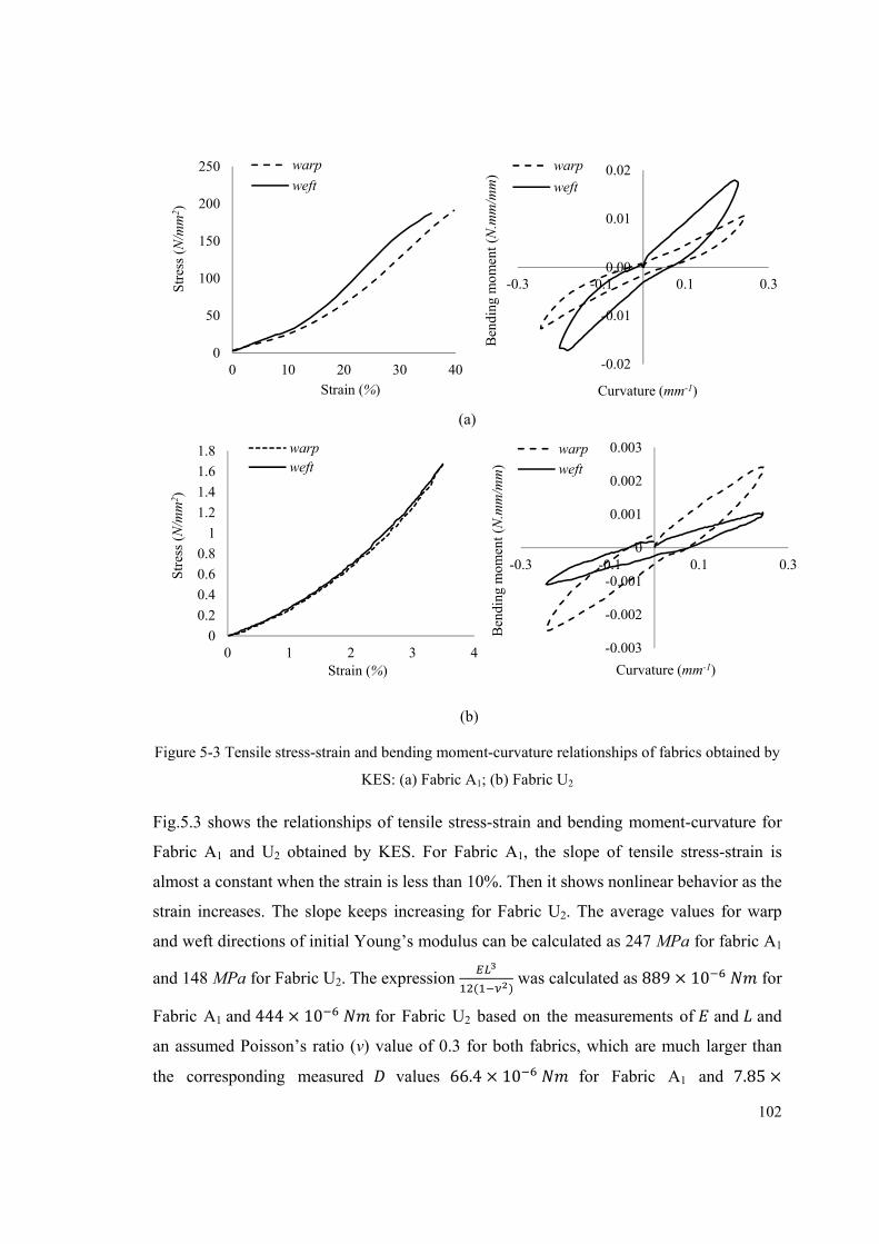
102

(a)

(b)

Figure 5-3 Tensile stress-strain and bending moment-curvature relationships of fabrics obtained by

KES: (a) Fabric A1; (b) Fabric U2

Fig.5.3 shows the relationships of tensile stress-strain and bending moment-curvature for

Fabric A1 and U2 obtained by KES. For Fabric A1, the slope of tensile stress-strain is

almost a constant when the strain is less than 10%. Then it shows nonlinear behavior as the

strain increases. The slope keeps increasing for Fabric U2. The average values for warp

and weft directions of initial Young’s modulus can be calculated as 247 MPa for fabric A1

and 148 MPa for Fabric U2. The expression ( ) was calculated as 889 × 10 for

Fabric A1 and 444 × 10 for Fabric U2 based on the measurements of and and

an assumed Poisson’s ratio (v) value of 0.3 for both fabrics, which are much larger than

the corresponding measured values 66.4 × 10 for Fabric A1 and 7.85 ×

0

50

100

150

200

250

0 10 20 30 40

Str

ess

(N/m

m2 )

Strain (%)

warp

weft

-0.02

-0.01

0.00

0.01

0.02

-0.3 -0.1 0.1 0.3

Ben

ding

mom

ent (

N.m

m/m

m)

Curvature (mm-1)

warp

weft

0

0.2

0.4

0.6

0.8

1

1.2

1.4

1.6

1.8

0 1 2 3 4

Str

ess

(N/m

m2 )

Strain (%)

warpweft

-0.003

-0.002

-0.001

0

0.001

0.002

0.003

-0.3 -0.1 0.1 0.3

Ben

ding

mom

ent (

N.m

m/m

m)

Curvature (mm-1)

warp

weft

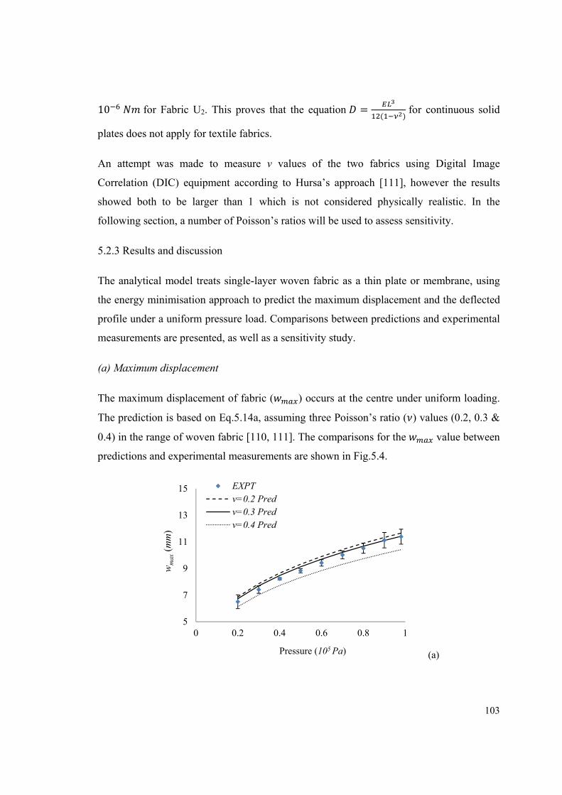
103

10 for Fabric U2. This proves that the equation = ( ) for continuous solid

plates does not apply for textile fabrics.

An attempt was made to measure v values of the two fabrics using Digital Image

Correlation (DIC) equipment according to Hursa’s approach [111], however the results

showed both to be larger than 1 which is not considered physically realistic. In the

following section, a number of Poisson’s ratios will be used to assess sensitivity.

5.2.3 Results and discussion

The analytical model treats single-layer woven fabric as a thin plate or membrane, using

the energy minimisation approach to predict the maximum displacement and the deflected

profile under a uniform pressure load. Comparisons between predictions and experimental

measurements are presented, as well as a sensitivity study.

(a) Maximum displacement

The maximum displacement of fabric ( ) occurs at the centre under uniform loading.

The prediction is based on Eq.5.14a, assuming three Poisson’s ratio ( ) values (0.2, 0.3 &

0.4) in the range of woven fabric [110, 111]. The comparisons for the value between

predictions and experimental measurements are shown in Fig.5.4.

(a)

5

7

9

11

13

15

0 0.2 0.4 0.6 0.8 1

wm

ax(m

m)

Pressure (105 Pa)

EXPTv=0.2 Predv=0.3 Predv=0.4 Pred

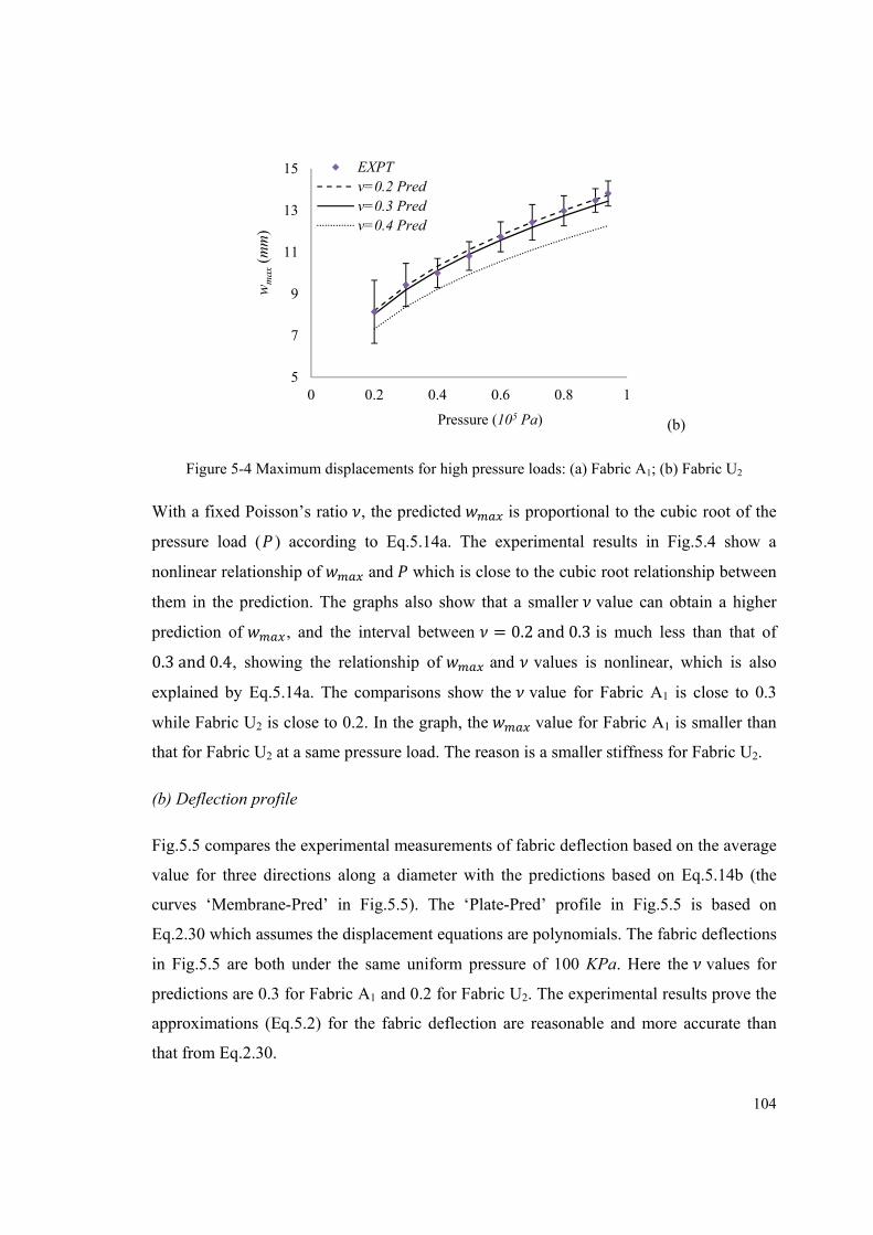
104

(b)

Figure 5-4 Maximum displacements for high pressure loads: (a) Fabric A1; (b) Fabric U2

With a fixed Poisson’s ratio , the predicted is proportional to the cubic root of the

pressure load ( ) according to Eq.5.14a. The experimental results in Fig.5.4 show a

nonlinear relationship of and which is close to the cubic root relationship between

them in the prediction. The graphs also show that a smaller value can obtain a higher

prediction of , and the interval between = 0.2and0.3 is much less than that of 0.3and0.4, showing the relationship of and values is nonlinear, which is also

explained by Eq.5.14a. The comparisons show the value for Fabric A1 is close to 0.3

while Fabric U2 is close to 0.2. In the graph, the value for Fabric A1 is smaller than

that for Fabric U2 at a same pressure load. The reason is a smaller stiffness for Fabric U2.

(b) Deflection profile

Fig.5.5 compares the experimental measurements of fabric deflection based on the average

value for three directions along a diameter with the predictions based on Eq.5.14b (the

curves ‘Membrane-Pred’ in Fig.5.5). The ‘Plate-Pred’ profile in Fig.5.5 is based on

Eq.2.30 which assumes the displacement equations are polynomials. The fabric deflections

in Fig.5.5 are both under the same uniform pressure of 100 KPa. Here the values for

predictions are 0.3 for Fabric A1 and 0.2 for Fabric U2. The experimental results prove the

approximations (Eq.5.2) for the fabric deflection are reasonable and more accurate than

that from Eq.2.30.

5

7

9

11

13

15

0 0.2 0.4 0.6 0.8 1

wm

ax(m

m)

Pressure (105 Pa)

EXPTv=0.2 Predv=0.3 Predv=0.4 Pred

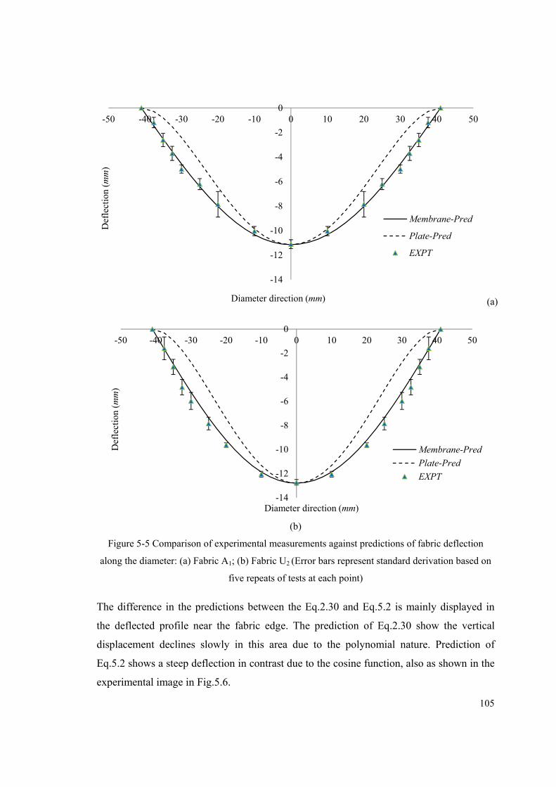
105

(a)

(b)

Figure 5-5 Comparison of experimental measurements against predictions of fabric deflection

along the diameter: (a) Fabric A1; (b) Fabric U2 (Error bars represent standard derivation based on

five repeats of tests at each point)

The difference in the predictions between the Eq.2.30 and Eq.5.2 is mainly displayed in

the deflected profile near the fabric edge. The prediction of Eq.2.30 show the vertical

displacement declines slowly in this area due to the polynomial nature. Prediction of

Eq.5.2 shows a steep deflection in contrast due to the cosine function, also as shown in the

experimental image in Fig.5.6.

-14

-12

-10

-8

-6

-4

-2

0-50 -40 -30 -20 -10 0 10 20 30 40 50

Def

lect

ion

(mm

)

Diameter direction (mm)

Membrane-Pred

Plate-Pred

EXPT

-14

-12

-10

-8

-6

-4

-2

0-50 -40 -30 -20 -10 0 10 20 30 40 50

Def

lect

ion

(mm

)

Diameter direction (mm)

Membrane-Pred

Plate-Pred

EXPT

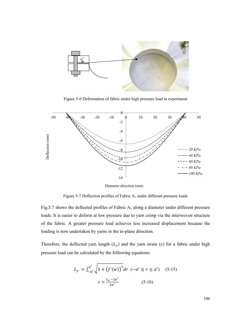
106

Figure 5-6 Deformation of fabric under high pressure load in experiment

Figure 5-7 Deflection profiles of Fabric A1 under different pressure loads

Fig.5.7 shows the deflected profiles of Fabric A1 along a diameter under different pressure

loads. It is easier to deform at low pressure due to yarn crimp via the interwoven structure

of the fabric. A greater pressure load achieves less increased displacement because the

loading is now undertaken by yarns in the in-plane direction.

Therefore, the deflected yarn length ( ) and the yarn strain ( ) for a fabric under high

pressure load can be calculated by the following equations:

= 1 + ′( ) (− ≤ ≤ ) (5-15) = (5-16)

-14

-12

-10

-8

-6

-4

-2

0-50 -40 -30 -20 -10 0 10 20 30 40 50

Def

lect

ion

(mm

)

Diameter direction (mm)

20 KPa

40 KPa

60 KPa

80 KPa

100 KPa

′

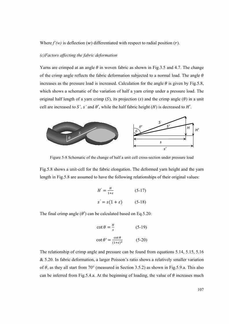
107

Where f’(w) is deflection ( ) differentiated with respect to radial position ( ).

(c)Factors affecting the fabric deformation

Yarns are crimped at an angle in woven fabric as shown in Fig.3.5 and 4.7. The change

of the crimp angle reflects the fabric deformation subjected to a normal load. The angle

increases as the pressure load is increased. Calculation for the angle is given by Fig.5.8,

which shows a schematic of the variation of half a yarn crimp under a pressure load. The

original half length of a yarn crimp ( ), its projection ( ) and the crimp angle ( ) in a unit

cell are increased to ’, ’ and ′, while the half fabric height ( ) is decreased to ′.

Figure 5-8 Schematic of the change of half a unit cell cross-section under pressure load

Fig.5.8 shows a unit-cell for the fabric elongation. The deformed yarn height and the yarn

length in Fig.5.8 are assumed to have the following relationships of their original values:

′ = (5-17)

′ = (1 + ) (5-18)

The final crimp angle ( ′) can be calculated based on Eq.5.20:

cot = (5-19)

cot ′ = ( ) (5-20)

The relationship of crimp angle and pressure can be found from equations 5.14, 5.15, 5.16

& 5.20. In fabric deformation, a larger Poisson’s ratio shows a relatively smaller variation

of , as they all start from 70° (measured in Section 3.5.2) as shown in Fig.5.9.a. This also

can be inferred from Fig.5.4.a. At the beginning of loading, the value of increases much

θθ'

SS’ H H’

s

s’

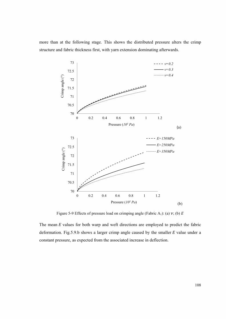
108

more than at the following stage. This shows the distributed pressure alters the crimp

structure and fabric thickness first, with yarn extension dominating afterwards.

(a)

(b)

Figure 5-9 Effects of pressure load on crimping angle (Fabric A1): (a) ; (b)

The mean values for both warp and weft directions are employed to predict the fabric

deformation. Fig.5.9.b shows a larger crimp angle caused by the smaller value under a

constant pressure, as expected from the associated increase in deflection.

70

70.5

71

71.5

72

72.5

73

0 0.2 0.4 0.6 0.8 1 1.2

Cri

mp

angl

e (°

)

Pressure (105 Pa)

v=0.2

v=0.3

v=0.4

70

70.5

71

71.5

72

72.5

73

0 0.2 0.4 0.6 0.8 1 1.2

Cri

mp

angl

e (°

)

Pressure (105 Pa)

E=150MPa

E=250MPa

E=350MPa

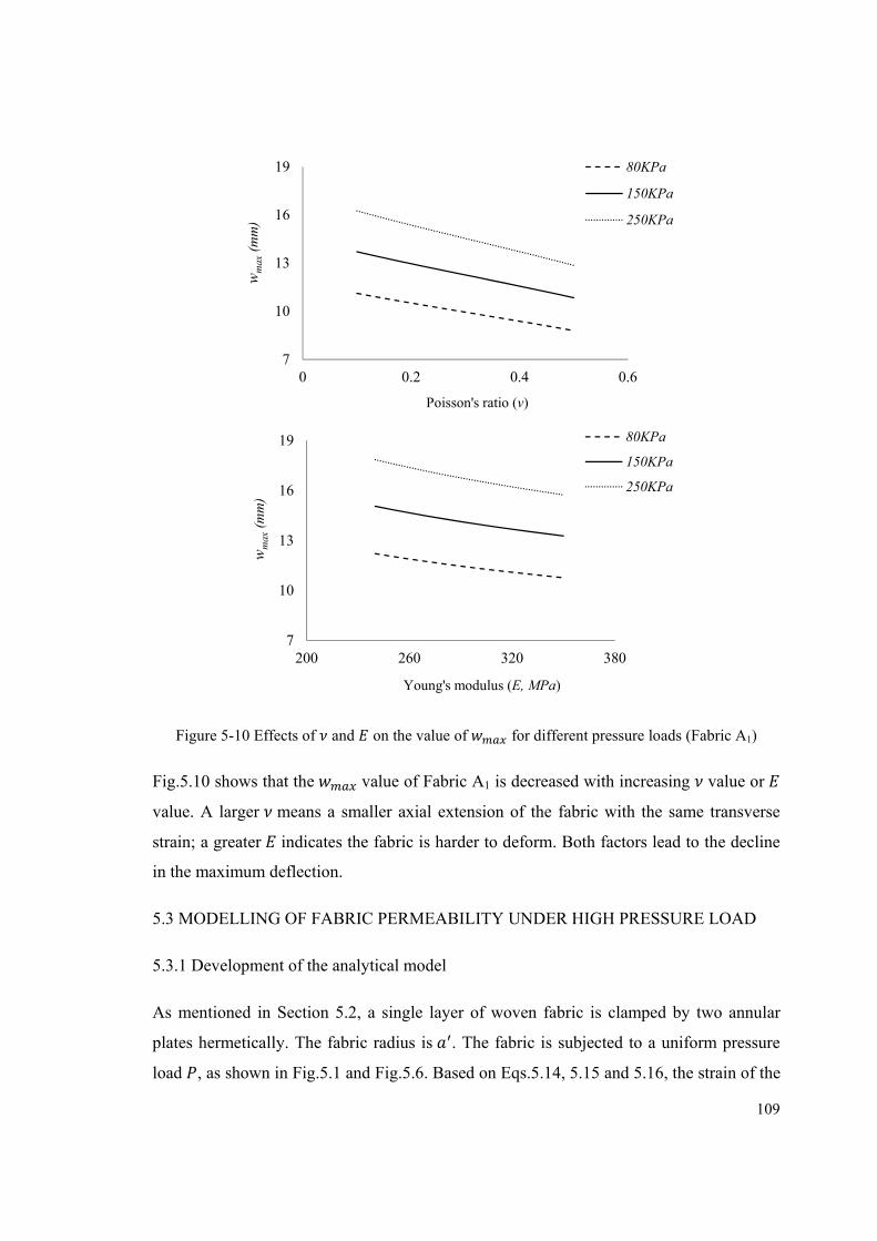
109

Figure 5-10 Effects of and on the value of for different pressure loads (Fabric A1)

Fig.5.10 shows that the value of Fabric A1 is decreased with increasing value or

value. A larger means a smaller axial extension of the fabric with the same transverse

strain; a greater indicates the fabric is harder to deform. Both factors lead to the decline

in the maximum deflection.

5.3 MODELLING OF FABRIC PERMEABILITY UNDER HIGH PRESSURE LOAD

5.3.1 Development of the analytical model

As mentioned in Section 5.2, a single layer of woven fabric is clamped by two annular

plates hermetically. The fabric radius is . The fabric is subjected to a uniform pressure

load , as shown in Fig.5.1 and Fig.5.6. Based on Eqs.5.14, 5.15 and 5.16, the strain of the

7

10

13

16

19

0 0.2 0.4 0.6

wm

ax(m

m)

Poisson's ratio (v)

80KPa

150KPa

250KPa

7

10

13

16

19

200 260 320 380

wm

ax(m

m)

Young's modulus (E, MPa)

80KPa

150KPa

250KPa

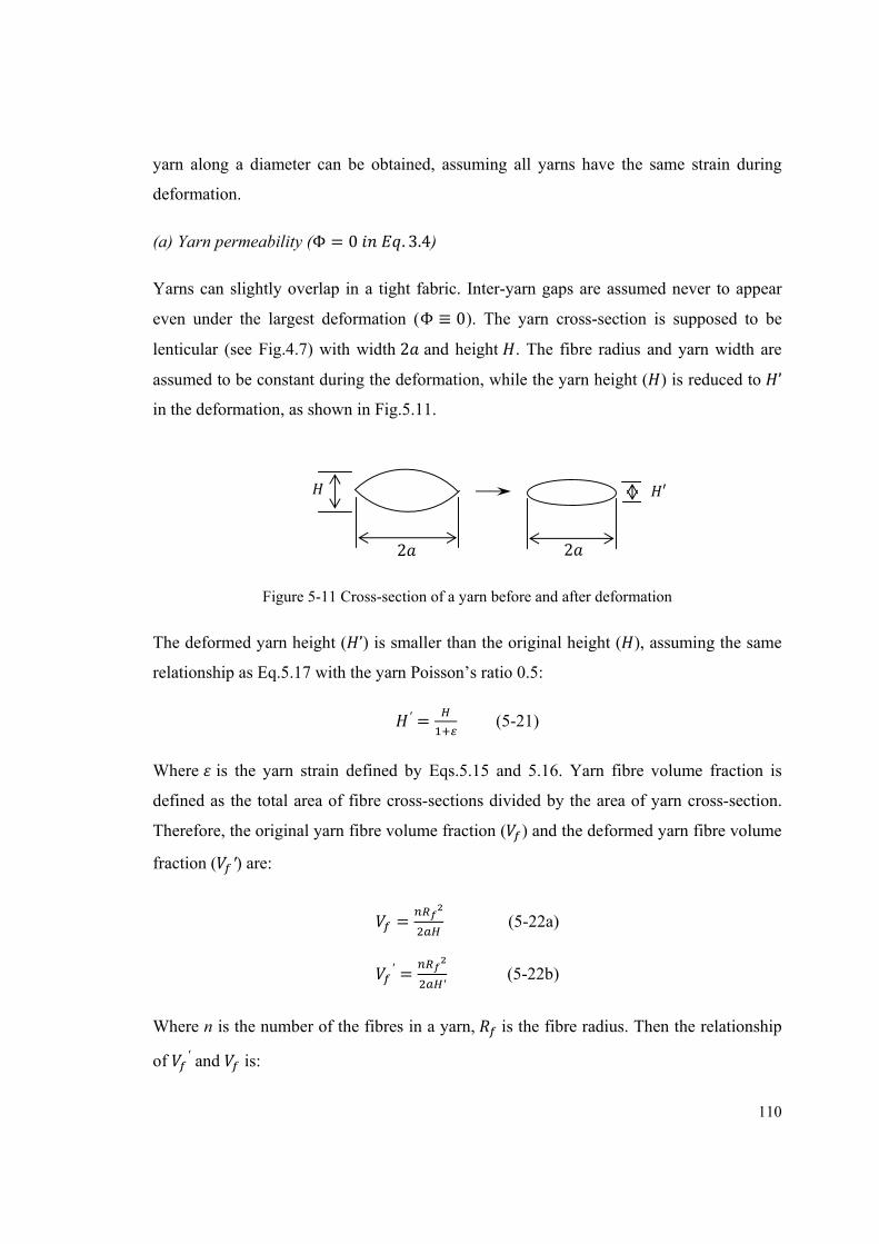
110

yarn along a diameter can be obtained, assuming all yarns have the same strain during

deformation.

(a) Yarn permeability (Φ = 0 . 3.4)

Yarns can slightly overlap in a tight fabric. Inter-yarn gaps are assumed never to appear

even under the largest deformation (Φ ≡ 0). The yarn cross-section is supposed to be

lenticular (see Fig.4.7) with width 2 and height . The fibre radius and yarn width are

assumed to be constant during the deformation, while the yarn height ( ) is reduced to ’ in the deformation, as shown in Fig.5.11.

Figure 5-11 Cross-section of a yarn before and after deformation

The deformed yarn height ( ’) is smaller than the original height ( ), assuming the same

relationship as Eq.5.17 with the yarn Poisson’s ratio 0.5:

′ = (5-21)

Where is the yarn strain defined by Eqs.5.15 and 5.16. Yarn fibre volume fraction is

defined as the total area of fibre cross-sections divided by the area of yarn cross-section.

Therefore, the original yarn fibre volume fraction ( ) and the deformed yarn fibre volume

fraction ( ′) are:

= (5-22a)

′ =′ (5-22b)

Where n is the number of the fibres in a yarn, is the fibre radius. Then the relationship

of ′ and is:

2

2′

111

′ = (1 + ) (5-23)

The yarns crimp angle can be calculated from Eqs.5.16, 5.19 and 5.20. Substitution of the

parameters ′ and ′ into Eq.3.10 allows the permeability of the deformed tight fabric to

be predicted theoretically.

(b) Gap permeability (Φ ≠ 0 . 3.4)

Along the fabric diameter, yarns are stretched under a strain ( ). The yarn cross-section is

assumed elliptical (see Appendix V). The yarn width is assumed constant (as demonstrated

in Table 4-4). The yarn height is assumed to decrease while the yarn length is increased.

The deformed yarn cross-section area ( ′) is:

′ = (5-24)

The yarn height ( ) is decreased:

′ = (5-25)

The deformed gap radius ( ′) between yarns is calculated as follows due to the stretched

yarn length:

′ = (1 + ) (5-26)

The curvature or shape factor ( ) of the flow channel in Eq.3.13 relates to the fabric

thickness:

′ = = (1 + ) (5-27)

Substitution of the parameters ′, ′ and ′ into Eq.3.23 allows the permeability of the

deformed loose fabric to be predicted by Eq.3.4 with new porosity theoretically.

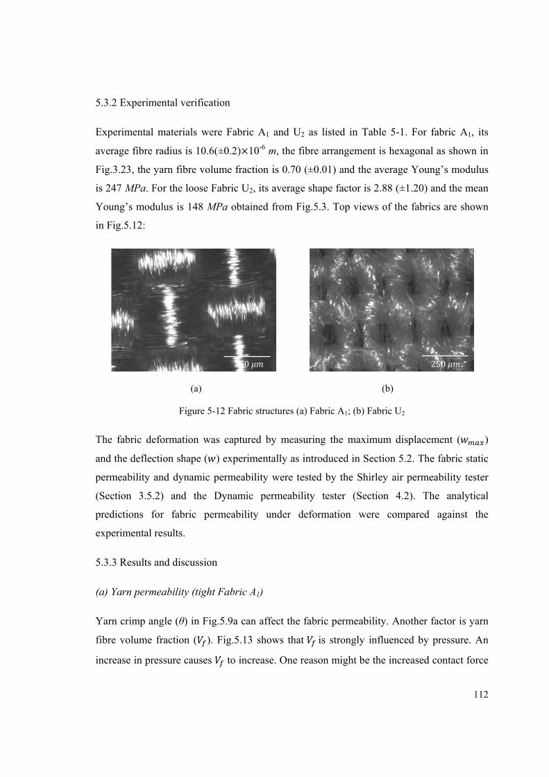
112

5.3.2 Experimental verification

Experimental materials were Fabric A1 and U2 as listed in Table 5-1. For fabric A1, its

average fibre radius is 10.6(±0.2)×10-6 m, the fibre arrangement is hexagonal as shown in

Fig.3.23, the yarn fibre volume fraction is 0.70 (±0.01) and the average Young’s modulus

is 247 MPa. For the loose Fabric U2, its average shape factor is 2.88 (±1.20) and the mean

Young’s modulus is 148 MPa obtained from Fig.5.3. Top views of the fabrics are shown

in Fig.5.12:

(a) (b)

Figure 5-12 Fabric structures (a) Fabric A1; (b) Fabric U2

The fabric deformation was captured by measuring the maximum displacement ( )

and the deflection shape ( ) experimentally as introduced in Section 5.2. The fabric static

permeability and dynamic permeability were tested by the Shirley air permeability tester

(Section 3.5.2) and the Dynamic permeability tester (Section 4.2). The analytical

predictions for fabric permeability under deformation were compared against the

experimental results.

5.3.3 Results and discussion

(a) Yarn permeability (tight Fabric A1)

Yarn crimp angle (θ) in Fig.5.9a can affect the fabric permeability. Another factor is yarn

fibre volume fraction ( ). Fig.5.13 shows that is strongly influenced by pressure. An

increase in pressure causes to increase. One reason might be the increased contact force

250250

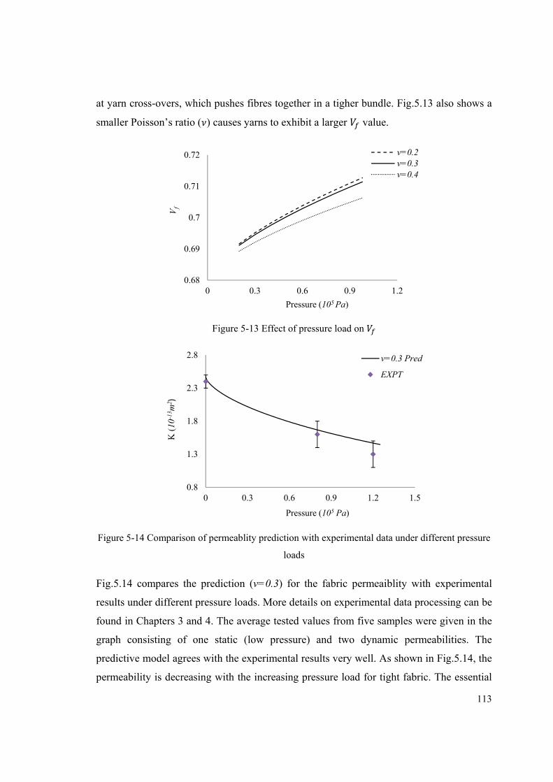
113

at yarn cross-overs, which pushes fibres together in a tigher bundle. Fig.5.13 also shows a

smaller Poisson’s ratio ( ) causes yarns to exhibit a larger value.

Figure 5-13 Effect of pressure load on

Figure 5-14 Comparison of permeablity prediction with experimental data under different pressure

loads

Fig.5.14 compares the prediction (v=0.3) for the fabric permeaiblity with experimental

results under different pressure loads. More details on experimental data processing can be

found in Chapters 3 and 4. The average tested values from five samples were given in the

graph consisting of one static (low pressure) and two dynamic permeabilities. The

predictive model agrees with the experimental results very well. As shown in Fig.5.14, the

permeability is decreasing with the increasing pressure load for tight fabric. The essential

0.68

0.69

0.7

0.71

0.72

0 0.3 0.6 0.9 1.2

Vf

Pressure (105 Pa)

v=0.2v=0.3v=0.4

0.8

1.3

1.8

2.3

2.8

0 0.3 0.6 0.9 1.2 1.5

K (

10-1

3 m2 )

Pressure (105 Pa)

v=0.3 Pred

EXPT

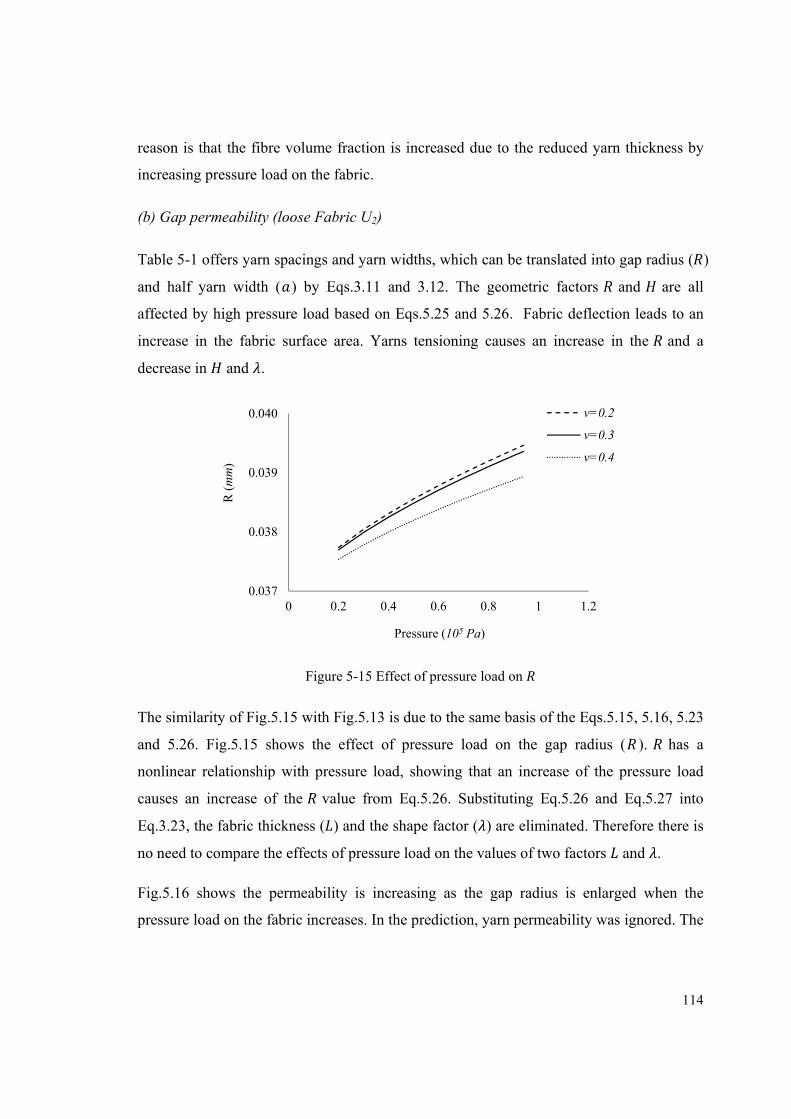
114

reason is that the fibre volume fraction is increased due to the reduced yarn thickness by

increasing pressure load on the fabric.

(b) Gap permeability (loose Fabric U2)

Table 5-1 offers yarn spacings and yarn widths, which can be translated into gap radius ( )

and half yarn width ( ) by Eqs.3.11 and 3.12. The geometric factors and are all

affected by high pressure load based on Eqs.5.25 and 5.26. Fabric deflection leads to an

increase in the fabric surface area. Yarns tensioning causes an increase in the and a

decrease in and .

Figure 5-15 Effect of pressure load on

The similarity of Fig.5.15 with Fig.5.13 is due to the same basis of the Eqs.5.15, 5.16, 5.23

and 5.26. Fig.5.15 shows the effect of pressure load on the gap radius ( ). has a

nonlinear relationship with pressure load, showing that an increase of the pressure load

causes an increase of the value from Eq.5.26. Substituting Eq.5.26 and Eq.5.27 into

Eq.3.23, the fabric thickness ( ) and the shape factor ( ) are eliminated. Therefore there is

no need to compare the effects of pressure load on the values of two factors and .

Fig.5.16 shows the permeability is increasing as the gap radius is enlarged when the

pressure load on the fabric increases. In the prediction, yarn permeability was ignored. The

0.037

0.038

0.039

0.040

0 0.2 0.4 0.6 0.8 1 1.2

R (

mm

)

Pressure (105 Pa)

v=0.2

v=0.3

v=0.4

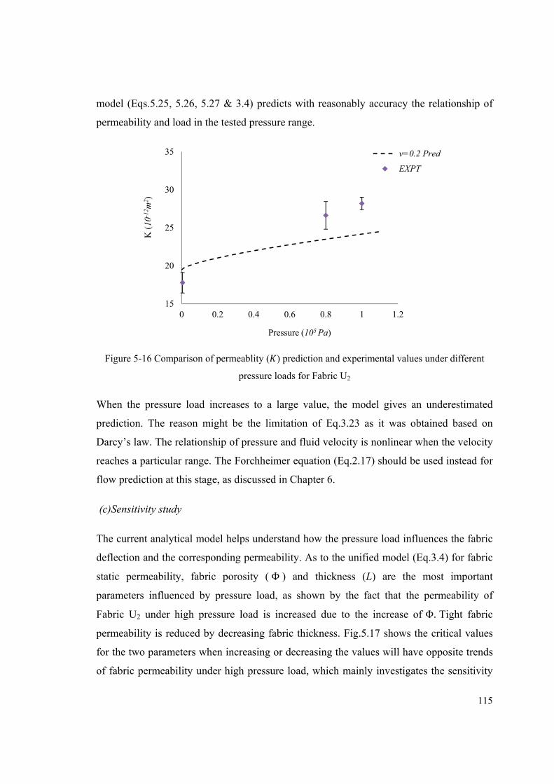
115

model (Eqs.5.25, 5.26, 5.27 & 3.4) predicts with reasonably accuracy the relationship of

permeability and load in the tested pressure range.

Figure 5-16 Comparison of permeablity ( ) prediction and experimental values under different

pressure loads for Fabric U2

When the pressure load increases to a large value, the model gives an underestimated

prediction. The reason might be the limitation of Eq.3.23 as it was obtained based on

Darcy’s law. The relationship of pressure and fluid velocity is nonlinear when the velocity

reaches a particular range. The Forchheimer equation (Eq.2.17) should be used instead for

flow prediction at this stage, as discussed in Chapter 6.

(c)Sensitivity study

The current analytical model helps understand how the pressure load influences the fabric

deflection and the corresponding permeability. As to the unified model (Eq.3.4) for fabric

static permeability, fabric porosity (Φ ) and thickness (L) are the most important

parameters influenced by pressure load, as shown by the fact that the permeability of

Fabric U2 under high pressure load is increased due to the increase of Φ. Tight fabric

permeability is reduced by decreasing fabric thickness. Fig.5.17 shows the critical values

for the two parameters when increasing or decreasing the values will have opposite trends

of fabric permeability under high pressure load, which mainly investigates the sensitivity

15

20

25

30

35

0 0.2 0.4 0.6 0.8 1 1.2

K (

10-1

2 m2 )

Pressure (105 Pa)

v=0.2 Pred

EXPT

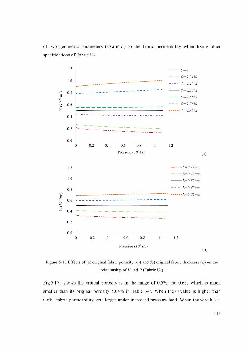
116

of two geometric parameters (Φand ) to the fabric permeability when fixing other

specifications of Fabric U2.

(a)

(b)

Figure 5-17 Effects of (a) original fabric porosity (Φ) and (b) original fabric thickness (L) on the

relationship of K and P (Fabric U2)

Fig.5.17a shows the critical porosity is in the range of 0.5% and 0.6% which is much

smaller than its original porosity 5.04% in Table 3-7. When the Φ value is higher than

0.6%, fabric permeability gets larger under increased pressure load. When the Φ value is

0.0

0.2

0.4

0.6

0.8

1.0

1.2

0 0.2 0.4 0.6 0.8 1 1.2

K (

10-1

2m

2 )

Pressure (105 Pa)

Φ=0

Φ=0.21%

Φ=0.46%

Φ=0.53%

Φ=0.58%

Φ=0.76%

Φ=0.85%

0.0

0.2

0.4

0.6

0.8

1.0

1.2

0 0.2 0.4 0.6 0.8 1 1.2

K (

10-1

2 m2 )

Pressure (105 Pa)

L=0.12mm

L=0.22mm

L=0.32mm

L=0.42mm

L=0.52mm

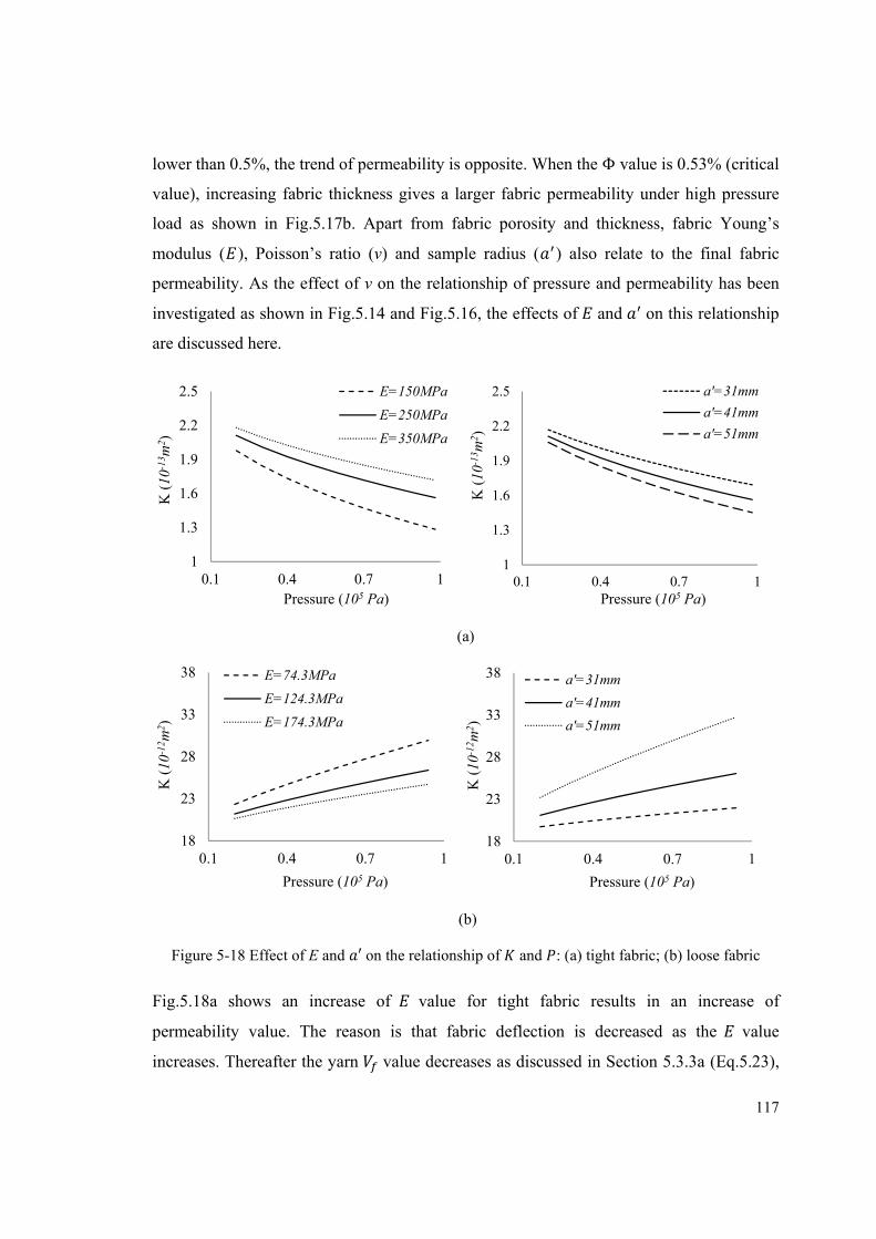
117

lower than 0.5%, the trend of permeability is opposite. When the Φ value is 0.53% (critical

value), increasing fabric thickness gives a larger fabric permeability under high pressure

load as shown in Fig.5.17b. Apart from fabric porosity and thickness, fabric Young’s

modulus ( ), Poisson’s ratio (v) and sample radius ( ) also relate to the final fabric

permeability. As the effect of v on the relationship of pressure and permeability has been

investigated as shown in Fig.5.14 and Fig.5.16, the effects of and on this relationship

are discussed here.

(a)

(b)

Figure 5-18 Effect of E and ′ on the relationship of and : (a) tight fabric; (b) loose fabric

Fig.5.18a shows an increase of value for tight fabric results in an increase of

permeability value. The reason is that fabric deflection is decreased as the value

increases. Thereafter the yarn value decreases as discussed in Section 5.3.3a (Eq.5.23),

1

1.3

1.6

1.9

2.2

2.5

0.1 0.4 0.7 1

K (

10-1

3 m2 )

Pressure (105 Pa)

E=150MPa

E=250MPa

E=350MPa

1

1.3

1.6

1.9

2.2

2.5

0.1 0.4 0.7 1

K (

10-1

3 m2 )

Pressure (105 Pa)

a'=31mm

a'=41mm

a'=51mm

18

23

28

33

38

0.1 0.4 0.7 1

K (

10-1

2 m2 )

Pressure (105 Pa)

E=74.3MPa

E=124.3MPa

E=174.3MPa

18

23

28

33

38

0.1 0.4 0.7 1

K (

10-1

2 m2 )

Pressure (105 Pa)

a'=31mm

a'=41mm

a'=51mm

118

leading to a higher permeability. However, the increase of is nonlinear with the increase

in . It also shows permeability is decreased with an increase of pressure load for a fixed

value. In Fig.5.18b, loose fabric has the opposite trend compared to tight fabric. The gap

radius is increased as E is decreased, leading to a larger fabric permeability value (Eq.3.23

& 3.4).

Fig.5.18 was also obtained by changing the sample radius ( ′) when other parameters are

fixed. An increase of ′ value will increase the maximum displacement ( ) of the

deformed fabric (Eqs.5.14) and the fabric elongation rate (Eqs.5.15 & 5.16), influencing

the final permeability. The permeability is decreased with increasing ′ value as the

value is increased for tight fabric. The difference of permeabilities between ′ = 41

and ′ = 51 is smaller than that of ′ = 31 and ′ = 41 , indicating a lower

effect of increasing ′ on decreasing the fabric permeability. Fig.5.18b shows the loose

fabric permeability is increased as its ′ value increases. The reason might be that is

getting larger relatively as the fabric is deformed more at a larger ′ value. The difference

of permeabilities between ′ = 31 and ′ = 41 is smaller than that of ′ =41 and ′ = 51 , predicting an increase of fabric radius will cause the fabric

permeability to increase further.

5.4 CONCLUSIONS

This chapter proposed predictive analytical models for the out-of-plane deformation of a

woven fabric and its corresponding through-thickness permeability when it was under a

high pressure load.

In the model of fabric deformation, an energy-based approach was utilized, which

consisted of bending energy, strain energy and work done by pressure. The fabric was

assumed to behave like a thin membrane as the maximum deflection was many times

larger than the fabric thickness. Minimization energy of the system was used to derive the

relationship of maximum displacement ( ) and pressure load (P). Fabric deflected

shape was characterized by the and a cosine function of the fabric radius.

119

The model for predicting permeability was based on the accurate prediction of the fabric

deformation. Also it relied on the accurate prediction of the static permeability (Eqs.3.4,

3.10 & 3.23). The hypothesis was that the yarn width was invariable during the

deformation. Yarn permeability was predicted by assuming the increased yarn fibre

volume fraction and crimp angle due to the decreased yarn height. Gap permeability was

predicted by assuming the increased gap radius due to the fabric deflection. Fabric

thickness was reduced by the same amount as yarn height. Fabric shape factor was

thereafter obtained based on the assumed equation 3.13 (Eq.5.27).

Three experiments were used to verify the analytical models. Fabric out-of-plane

deformation was measured by a fabric deflection tester, with loading applied by a vacuum

pump. Fabric static permeability was determined by a Shirley air permeability tester while

fabric dynamic permeability was tested by a dynamic permeability tester. The predictions

of fabric deflection configurations (tight and loose fabrics) agree with the experimental

measurements very well. The deflection causes the yarn fibre volume fraction to increase

as well as the crimp angle, causing the permeability of tight fabric to decrease (Fig.5.14).

In contrast, the deflection leads to the gap radius to increase, obtaining an increased

permeability of loose fabric (Fig.5.16). The permeability predictions under high pressure

load agree with the experimental values well. Sensitivity studies firstly investigate the

critical fabric porosity and the critical fabric thickness where the increase or decrease of

fabric permeability occurs during the fabric deformation, and secondly show the fabric

properties, such as Young’s modulus, affect the fabric deformation, leading to an increase

in tight fabric permeability and a decrease in loose fabric permeability with increasing

modulus when the fabric is under the same pressure load. The model assists with

understanding the factors affecting the fabric permeability when the fabric is under high

pressure load, such as the change of airbag fabric permeability under inflation. The next

chapter will attempt to understand fabric permeability as affected by its flow channel

shape when the fabric is under high pressure drop.

120

CHAPTER 6

MODELLING OF NON-DARCY FLOW IN TEXTILES

6.1 INTRODUCTION

Fabric permeability describes the fabric resistance to flow in a hydraulic environment. The

relationship of pressure gradient and fluid velocity reflects a transfer from fluid potential

energy to flow kinetic energy. In Section 2.2 and 2.3, Darcy’s law and the Forchheimer

equation were reviewed, showing linear and nonlinear relationships respectively. Darcy’s

law is a special case of the Forchheimer equation when the Reynolds number ( ) is so

small that the term of second order of velocity can be ignored (typically < 10 100)

[84-85]. Therefore, a critical valule governs when to apply Darcy’s law or the

Forchheimer equation such as a criterion for the critical proposed by Zeng [84]. The

value of depends on the shape of the flow channel. This chapter takes into account two

geometries simplified from a woven fabric: a gradual converging-diverging tube and a

gradual converging-diverging pair of plates, which closely represent the inter-yarn gap in a

loose fabric and the space between two parallel unidirectional fibres in a yarn.

The coefficients in the Forchheimer equation are required to be quantified as a function of

geometric parameters of the flow channel. The developed model is expected to predict the

non-linear flow resistance based on flow channel geometry. Verification of the model is

carried out by CFD simulations, experiments and published experimental data. The

analysis also clarifies what is dominant in the nonlinear relationship of pressure and fluid

velocity: fabric deformation or shape of flow channel.

6.2 ANALYSIS OF NON-DARCY FLOW

6.2.1 Hagen-Poiseuille flow in gradual converging-diverging channels

For Newtonian fluids, the theory of fluid mechanics [63] gives closed-form solutions for

Hagen-Poiseuille flow in a long straight tube (Eq.6.1) or between two infinitely-long

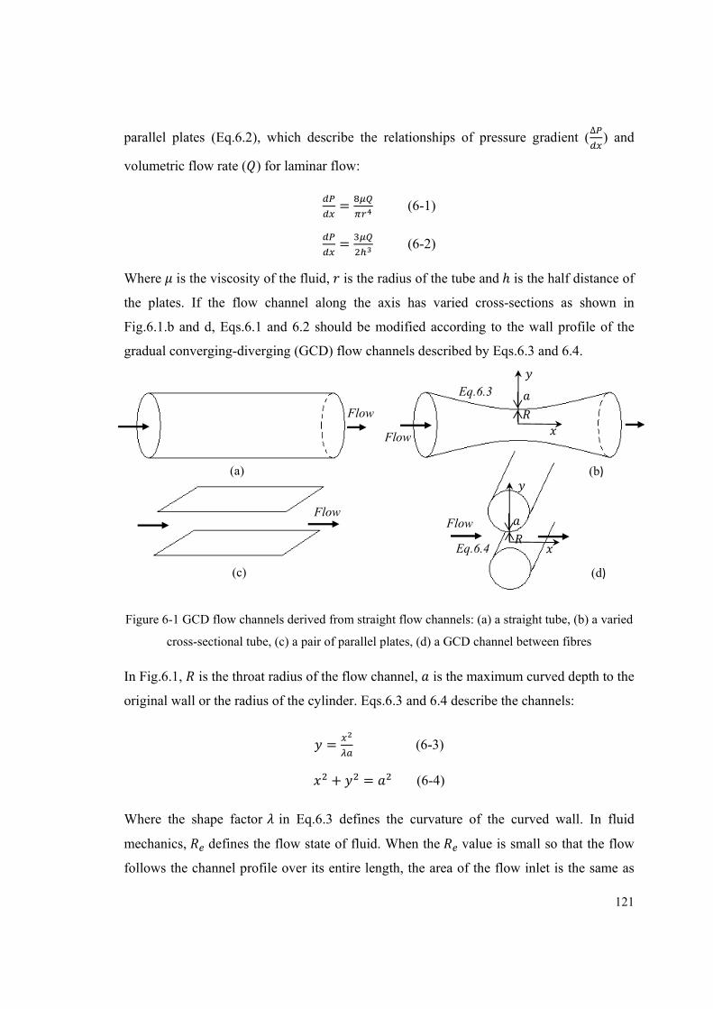
121

parallel plates (Eq.6.2), which describe the relationships of pressure gradient (∆

) and

volumetric flow rate ( ) for laminar flow:

= (6-1) = (6-2)

Where is the viscosity of the fluid, is the radius of the tube andℎ is the half distance of

the plates. If the flow channel along the axis has varied cross-sections as shown in

Fig.6.1.b and d, Eqs.6.1 and 6.2 should be modified according to the wall profile of the

gradual converging-diverging (GCD) flow channels described by Eqs.6.3 and 6.4.

Figure 6-1 GCD flow channels derived from straight flow channels: (a) a straight tube, (b) a varied

cross-sectional tube, (c) a pair of parallel plates, (d) a GCD channel between fibres

In Fig.6.1, is the throat radius of the flow channel, is the maximum curved depth to the

original wall or the radius of the cylinder. Eqs.6.3 and 6.4 describe the channels:

= (6-3) + = (6-4)

Where the shape factor in Eq.6.3 defines the curvature of the curved wall. In fluid

mechanics, defines the flow state of fluid. When the value is small so that the flow

follows the channel profile over its entire length, the area of the flow inlet is the same as

Eq.6.4

Flow

Flow

Flow

Flow

Eq.6.3

(a) (b)

(c) (d)

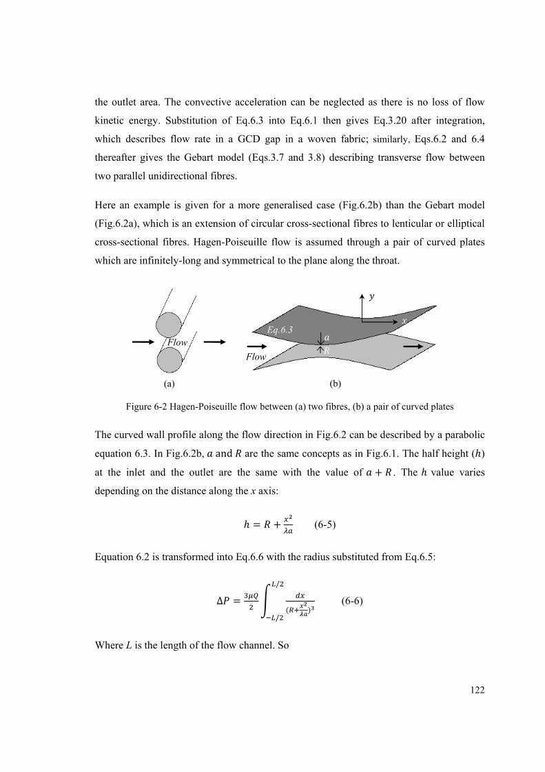
122

the outlet area. The convective acceleration can be neglected as there is no loss of flow

kinetic energy. Substitution of Eq.6.3 into Eq.6.1 then gives Eq.3.20 after integration,

which describes flow rate in a GCD gap in a woven fabric; similarly, Eqs.6.2 and 6.4

thereafter gives the Gebart model (Eqs.3.7 and 3.8) describing transverse flow between

two parallel unidirectional fibres.

Here an example is given for a more generalised case (Fig.6.2b) than the Gebart model

(Fig.6.2a), which is an extension of circular cross-sectional fibres to lenticular or elliptical

cross-sectional fibres. Hagen-Poiseuille flow is assumed through a pair of curved plates

which are infinitely-long and symmetrical to the plane along the throat.

Figure 6-2 Hagen-Poiseuille flow between (a) two fibres, (b) a pair of curved plates

The curved wall profile along the flow direction in Fig.6.2 can be described by a parabolic

equation 6.3. In Fig.6.2b, and are the same concepts as in Fig.6.1. The half height (ℎ)

at the inlet and the outlet are the same with the value of + . The ℎ value varies

depending on the distance along the x axis:

ℎ = + (6-5)

Equation 6.2 is transformed into Eq.6.6 with the radius substituted from Eq.6.5:

∆ = ( )// (6-6)

Where L is the length of the flow channel. So

Flow

(a) (b)

Flow

Eq.6.3

123

∆ = √ √( ( ) ) (6-7)

Setting = √ , then the integration in Eq.6.7 has the following solution:

( )√√ = ( ) + 3 tan √√ (6-8)

If the integral limit ( √ ) value in Eq.6.8 was set to more than 3 (shown in Fig.3.10), the

integration would approximately be . This was used instead of the complicated

expression (6.8). Accordingly, Eq.6.7 was simplified significantly with the solution:

∆ = √ (6-9)

When = 2 in Eq.6.9, it equals to the Gebart model as Eq.IV.6a. Eq.3.21 and Eq.6.9 both

show the linear relationship of pressure drop and volumetric flow rate. Combination with

Darcy’s law (Eq.1.1), Eqs.3.21 and 6.9 can predict the permeability ( ) accurately for

these geometries in textiles when is small.

6.2.2 Non-Darcy flow from Navier-Stokes Equation

The Navier-Stokes equation arises from applying Newton's second law to fluid motion,

together with the assumption that the fluid stress is the sum of a diffusing viscous term

(proportional to the gradient of velocity), plus a pressure term. It is a universal governing

equation in fluid mechanics, which has been introduced in Appendix II-c in detail. For an

incompressible Newtonian fluid it is given in Cartesian notation by:

+ ∙ ∇ = −∇ + ∇ + (6-10)

Where is the unsteady acceleration, ∙ ∇ is the convective acceleration, ∇ is the

pressure gradient, ∇ is the viscous force and is the other body force such as gravity.

The function for the shape of streamlines is fixed when flow is under constant pressure

124

gradient at a steady state, assuming is zero, for an arbitrary GCD flow channel, so

Eq.6.10 can be simplified as: ( ∙ ∇ ) = −∇ + ∇ (6-11)

As GCD flow channels are axisymmetric, 2D coordinates can be used for the channels in

Fig.6.1. The conditions for Eq.6.11 based on the geometries are:

≠ 0; ≠ 0; ≠ 0; Eq.6.11 is then expressed as:

= − + (6-12)

Where in Eq.6.12 is a symbol for the average velocity tensor. It has two components in

directions and . Integrating Eq.6.12 along the axis:

∆ = − + (6-13)

Equation 6.13 shows two parts of the pressure loss. The first part is the local pressure loss

depending on the channel geometry (Eq.6.14a), the appearance of it is from convective

acceleration depending on the variation of flow streamlines. The second part is the

frictional pressure loss based on the interaction of fluid and channel surface as well as the

fluid internal frictional force (Eq.6.14b): ∆ = − (6-14a) ∆ = (6-14b)

The two expressions in Eq.6.14 can be derived separately as they focus on linear and

nonlinear flow velocity terms respectively.

6.2.3 Analytical modelling of Non-Darcy flow

When of a fluid motion is very small, the fluid flows across the whole channel as

shown in Fig.6.3a. This is frequently come across when considering continuity theory (see

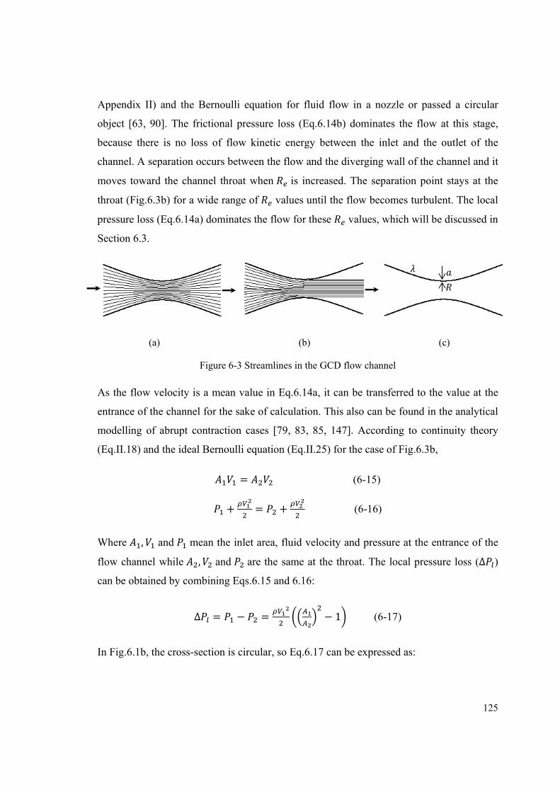
125

Appendix II) and the Bernoulli equation for fluid flow in a nozzle or passed a circular

object [63, 90]. The frictional pressure loss (Eq.6.14b) dominates the flow at this stage,

because there is no loss of flow kinetic energy between the inlet and the outlet of the

channel. A separation occurs between the flow and the diverging wall of the channel and it

moves toward the channel throat when is increased. The separation point stays at the

throat (Fig.6.3b) for a wide range of values until the flow becomes turbulent. The local

pressure loss (Eq.6.14a) dominates the flow for these values, which will be discussed in

Section 6.3.

(a) (b) (c)

Figure 6-3 Streamlines in the GCD flow channel

As the flow velocity is a mean value in Eq.6.14a, it can be transferred to the value at the

entrance of the channel for the sake of calculation. This also can be found in the analytical

modelling of abrupt contraction cases [79, 83, 85, 147]. According to continuity theory

(Eq.II.18) and the ideal Bernoulli equation (Eq.II.25) for the case of Fig.6.3b, = (6-15) + = + (6-16)

Where , and mean the inlet area, fluid velocity and pressure at the entrance of the

flow channel while , and are the same at the throat. The local pressure loss (∆ )

can be obtained by combining Eqs.6.15 and 6.16:

∆ = − = − 1 (6-17)

In Fig.6.1b, the cross-section is circular, so Eq.6.17 can be expressed as:

126

∆ = − 1 (6-18)

In Fig.6.1d or Fig.6.2, the cross-section is parallel walls, so Eq.6.17 can be expressed as:

∆ = − 1 (6-19)

As for the frictional pressure loss, Eq.6.14b can be integrated based on detailed boundary

conditions. The GCD tube and plates (Eqs.3.11 & 6.9) are merely two cases obtained

using the integration of Eq.6.14b. Pipes, tubes, nozzles or diffusers all have frictional force

components to the flow. For instance, the frictional factor for a straight tube based on the

Hagen-Poisseuille equation (Eq.6.1) and the Dacry-Weisbach equation (6.20) [63]:

∆ = (6-20)

Where is the frictional factor, is the tube radius, is the tube length. Combination of

Eq.6.1 and Eq.6.20 has the frictional pressure loss for a straight tube:

∆ = (6-21)

Where = 2 ⁄ . As to the GCD flow channels, similar processing can be done as for

Eq.6.21. For the tube geometry like Fig.6.1b, Eq.3.21 can be rearranged into:

∆ = ( ) √ = ( ) √ (6-22)

Where the definition of is:

= ( ) (6-23)

Eq.6.22 reflects that the frictional pressure potential can be transformed into a flow kinetic

energy based on fluid property such as fluid viscosity and flow channel geometry such as

curvature. The total pressure loss for this GCD tube is obtained by combining Eq.6.18 and

Eq.6.22:

127

∆ = ( ) √ + { − 1} (6-24a)

The coefficient of hydraulic resistance ( ), defined as the ratio of the total pressure loss

(potential energy) to kinetic energy [148], reflects the transformation ability of the two

energies for a GCD flow channel. For a GCD tube, it is from Eq.6.24a:

= ∆ = ( ) √ + − 1 (6-24b)

For a channel geometry like Fig.6.2, Eq.6.9 can be transformed into:

∆ = ( )√ = ( ) √ (6-25)

Where is defined by Eq.6.23. Therefore the total pressure loss and the coefficient of

hydraulic resistance for this GCD channel are:

∆ = ( )√ + { − 1} (6-26a)

= ∆ = ( ) √ + − 1 (6-26b)

Both demonstrate a quadratic dependence of pressure drop on velocity, as described by the

Forchheimer equation (Eq.2.17). Eqs.6.24 and 6.26 are suitable for a value larger than

the critical value for flow separation at the throat region of the flow channel. A larger

value of hydraulic resistance means a lower flow rate through the channel under the same

pressure drop.

6.2.4 Hydraulic resistance of woven fabric

In a woven fabric, the gap between yarns in a unit cell forms a GCD flow tube. The fabric

porosity (Ф) is defined as the cross-sectional area of the throat divided by the cross-

sectional area of the inlet (2D unit-cell geometry in Fig.3.1):

Ф = 1(1+ )2 (6-27)

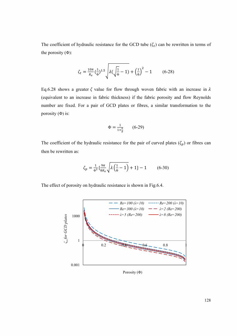
128

The coefficient of hydraulic resistance for the GCD tube ( ) can be rewritten in terms of

the porosity (Ф):

= (Ф) . ( Ф − 1) + Ф − 1 (6-28)

Eq.6.28 shows a greater value for flow through woven fabric with an increase in

(equivalent to an increase in fabric thickness) if the fabric porosity and flow Reynolds

number are fixed. For a pair of GCD plates or fibres, a similar transformation to the

porosity (Ф) is:

Ф = 11+ (6-29)

The coefficient of the hydraulic resistance for the pair of curved plates ( ) or fibres can

then be rewritten as:

= Ф { Ф − 1 + 1} − 1 (6-30)

The effect of porosity on hydraulic resistance is shown in Fig.6.4.

0.001

1

1000

0 0.2 0.4 0.6 0.8 1

ζ αfo

r G

CD

pla

tes

Porosity (Φ)

Re=100 (λ=10) Re=200 (λ=10)

Re=300 (λ=10) λ=2 (Re=200)

λ=5 (Re=200) λ=8 (Re=200)

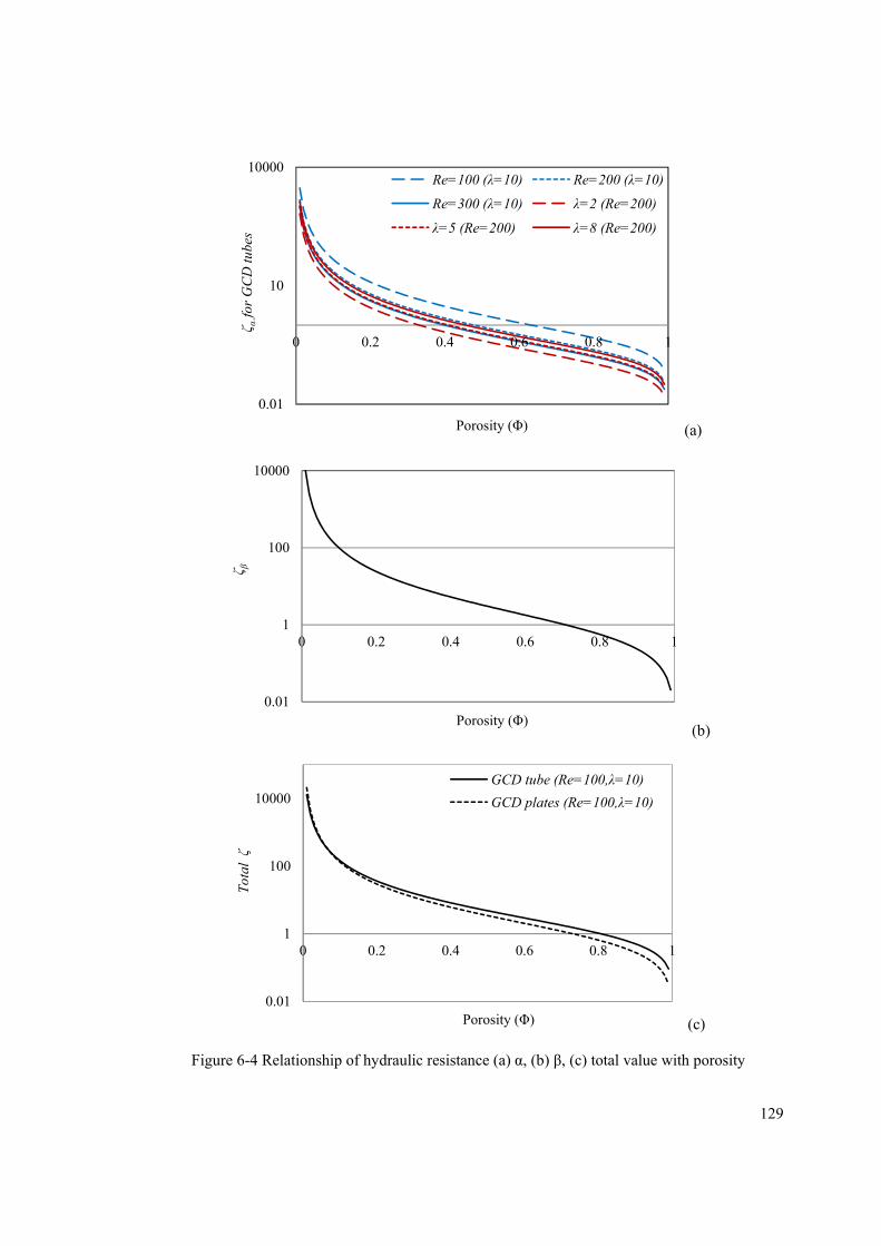
129

(a)

(b)

(c)

Figure 6-4 Relationship of hydraulic resistance (a) α, (b) β, (c) total value with porosity

0.01

10

10000

0 0.2 0.4 0.6 0.8 1

ζ αfo

r G

CD

tube

s

Porosity (Φ)

Re=100 (λ=10) Re=200 (λ=10)

Re=300 (λ=10) λ=2 (Re=200)

λ=5 (Re=200) λ=8 (Re=200)

0.01

1

100

10000

0 0.2 0.4 0.6 0.8 1

ζ β

Porosity (Φ)

0.01

1

100

10000

0 0.2 0.4 0.6 0.8 1

Tota

l ζ

Porosity (Φ)

GCD tube (Re=100,λ=10)

GCD plates (Re=100,λ=10)

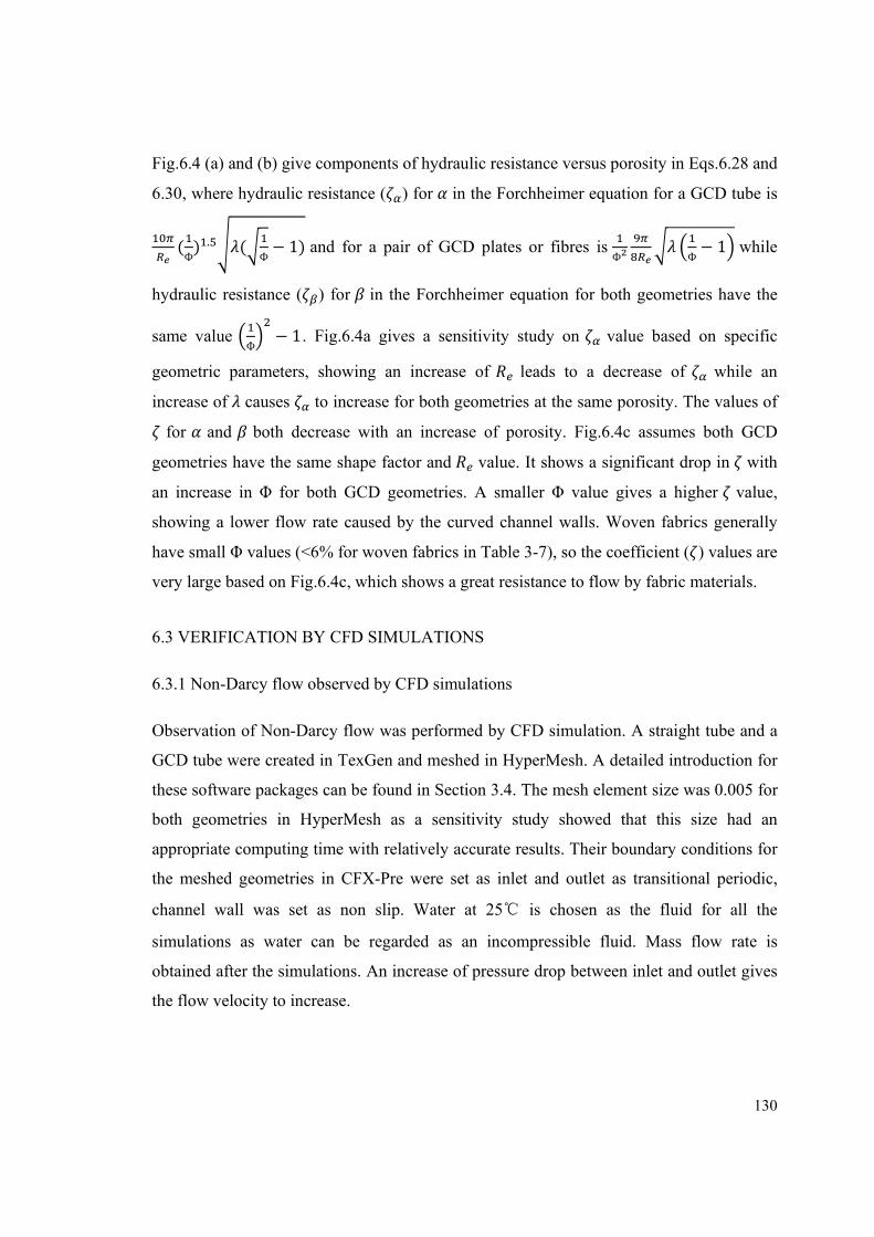
130

Fig.6.4 (a) and (b) give components of hydraulic resistance versus porosity in Eqs.6.28 and

6.30, where hydraulic resistance ( ) for in the Forchheimer equation for a GCD tube is

(Ф) . ( Ф − 1) and for a pair of GCD plates or fibres is Ф Ф − 1 while

hydraulic resistance ( ) for in the Forchheimer equation for both geometries have the

same value Ф − 1. Fig.6.4a gives a sensitivity study on value based on specific

geometric parameters, showing an increase of leads to a decrease of while an

increase of causes to increase for both geometries at the same porosity. The values of

for and both decrease with an increase of porosity. Fig.6.4c assumes both GCD

geometries have the same shape factor and value. It shows a significant drop in with

an increase in Φ for both GCD geometries. A smaller Φ value gives a higher value,

showing a lower flow rate caused by the curved channel walls. Woven fabrics generally

have small Φ values (<6% for woven fabrics in Table 3-7), so the coefficient ( ) values are

very large based on Fig.6.4c, which shows a great resistance to flow by fabric materials.

6.3 VERIFICATION BY CFD SIMULATIONS

6.3.1 Non-Darcy flow observed by CFD simulations

Observation of Non-Darcy flow was performed by CFD simulation. A straight tube and a

GCD tube were created in TexGen and meshed in HyperMesh. A detailed introduction for

these software packages can be found in Section 3.4. The mesh element size was 0.005 for

both geometries in HyperMesh as a sensitivity study showed that this size had an

appropriate computing time with relatively accurate results. Their boundary conditions for

the meshed geometries in CFX-Pre were set as inlet and outlet as transitional periodic,

channel wall was set as non slip. Water at 25℃ is chosen as the fluid for all the

simulations as water can be regarded as an incompressible fluid. Mass flow rate is

obtained after the simulations. An increase of pressure drop between inlet and outlet gives

the flow velocity to increase.

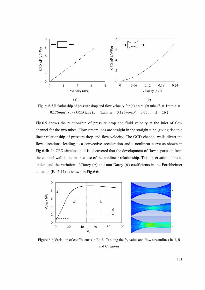
131

(a) (b)

Figure 6-5 Relationship of pressure drop and flow velocity for (a) a straight tube ( = 1 , =0.175 ); (b) a GCD tube ( = 1 , = 0.125 , = 0.05 , = 16 )

Fig.6.5 shows the relationship of pressure drop and fluid velocity at the inlet of flow

channel for the two tubes. Flow streamlines are straight in the straight tube, giving rise to a

linear relationship of pressure drop and flow velocity. The GCD channel walls divert the

flow directions, leading to a convective acceleration and a nonlinear curve as shown in

Fig.6.5b. In CFD simulation, it is discovered that the development of flow separation from

the channel wall is the main cause of the nonlinear relationship. This observation helps to

understand the variation of Darcy ( ) and non-Darcy ( ) coefficients in the Forchheimer

equation (Eq.2.17) as shown in Fig.6.6:

Figure 6-6 Variation of coefficients (in Eq.2.17) along the value and flow streamlines in A, B

and C regions

0

2

4

6

8

10

0 1 2 3 4

CFD

∆P

(103 P

a)

Velocity (m/s)

0

2

4

6

8

0 0.06 0.12 0.18 0.24

CFD

∆P

(10

3 Pa)

Velocity (m/s)

0

2

4

6

8

10

0 20 40 60 80 100

Val

ue (

104 )

Re

βα

A

B C

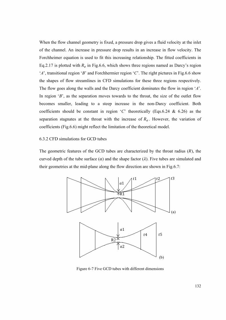
132

When the flow channel geometry is fixed, a pressure drop gives a fluid velocity at the inlet

of the channel. An increase in pressure drop results in an increase in flow velocity. The

Forchheimer equation is used to fit this increasing relationship. The fitted coefficients in

Eq.2.17 is plotted with in Fig.6.6, which shows three regions named as Darcy’s region

‘A’, transitional region ‘B’ and Forchhermier region ‘C’. The right pictures in Fig.6.6 show

the shapes of flow streamlines in CFD simulations for these three regions respectively.

The flow goes along the walls and the Darcy coefficient dominates the flow in region ‘A’.

In region ‘B’, as the separation moves towards to the throat, the size of the outlet flow

becomes smaller, leading to a steep increase in the non-Darcy coefficient. Both

coefficients should be constant in region ‘C’ theoretically (Eqs.6.24 & 6.26) as the

separation stagnates at the throat with the increase of . However, the variation of

coefficients (Fig.6.6) might reflect the limitation of the theoretical model.

6.3.2 CFD simulations for GCD tubes

The geometric features of the GCD tubes are characterized by the throat radius ( ), the

curved depth of the tube surface ( ) and the shape factor ( ). Five tubes are simulated and

their geometries at the mid-plane along the flow direction are shown in Fig.6.7:

(a)

(b)

Figure 6-7 Five GCD tubes with different dimensions

11R1

2 3

12R2

4 5

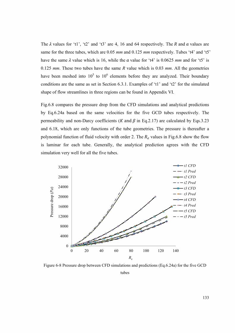
133

The values for ‘t1’, ‘t2’ and ‘t3’ are 4, 16 and 64 respectively. The and values are

same for the three tubes, which are 0.05 mm and 0.125 mm respectively. Tubes ‘t4’ and ‘t5’

have the same value which is 16, while the value for ‘t4’ is 0.0625 mm and for ‘t5’ is

0.125 mm. These two tubes have the same R value which is 0.03 mm. All the geometries

have been meshed into 105 to 106 elements before they are analyzed. Their boundary

conditions are the same as set in Section 6.3.1. Examples of ‘t1’ and ‘t2’ for the simulated

shape of flow streamlines in three regions can be found in Appendix VI.

Fig.6.8 compares the pressure drop from the CFD simulations and analytical predictions

by Eq.6.24a based on the same velocities for the five GCD tubes respectively. The

permeability and non-Darcy coefficients ( and in Eq.2.17) are calculated by Eqs.3.23

and 6.18, which are only functions of the tube geometries. The pressure is thereafter a

polynomial function of fluid velocity with order 2. The values in Fig.6.8 show the flow

is laminar for each tube. Generally, the analytical prediction agrees with the CFD

simulation very well for all the five tubes.

Figure 6-8 Pressure drop between CFD simulations and predictions (Eq.6.24a) for the five GCD

tubes

0

4000

8000

12000

16000

20000

24000

28000

32000

0 20 40 60 80 100 120 140

Pres

sure

dro

p (P

a)

Re

t1 CFD

t1 Pred

t2 CFD

t2 Pred

t3 CFD

t3 Pred

t4 CFD

t4 Pred

t5 CFD

t5 Pred

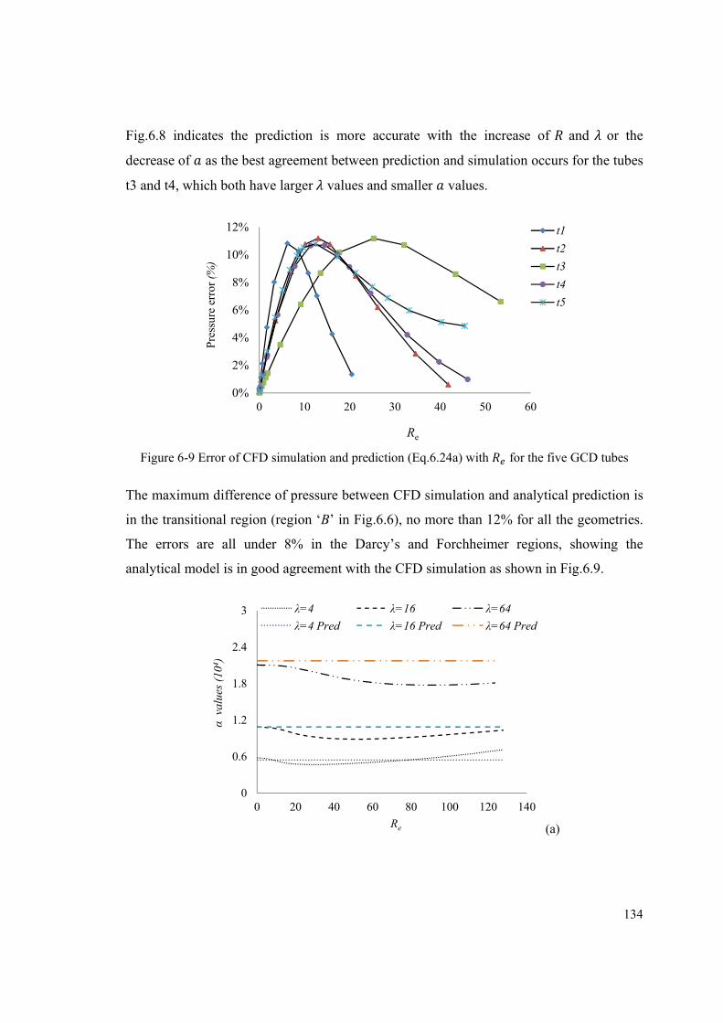
134

Fig.6.8 indicates the prediction is more accurate with the increase of and or the

decrease of as the best agreement between prediction and simulation occurs for the tubes

t3 and t4, which both have larger values and smaller values.

Figure 6-9 Error of CFD simulation and prediction (Eq.6.24a) with for the five GCD tubes

The maximum difference of pressure between CFD simulation and analytical prediction is

in the transitional region (region ‘B’ in Fig.6.6), no more than 12% for all the geometries.

The errors are all under 8% in the Darcy’s and Forchheimer regions, showing the

analytical model is in good agreement with the CFD simulation as shown in Fig.6.9.

(a)

0%

2%

4%

6%

8%

10%

12%

0 10 20 30 40 50 60

Pre

ssur

e er

ror

(%)

Re

t1

t2

t3

t4

t5

0

0.6

1.2

1.8

2.4

3

0 20 40 60 80 100 120 140

αva

lues

(10

4 )

Re

λ=4 λ=16 λ=64

λ=4 Pred λ=16 Pred λ=64 Pred

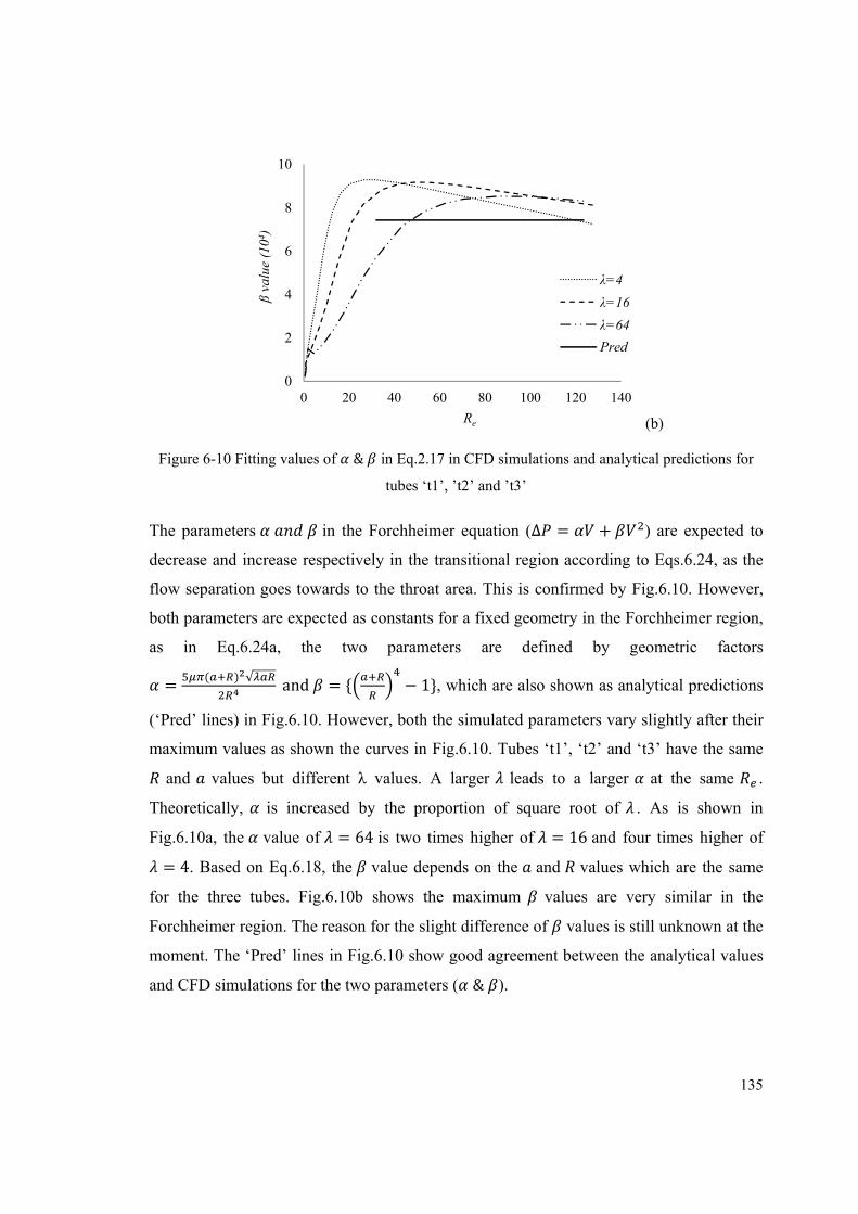
135

(b)

Figure 6-10 Fitting values of & in Eq.2.17 in CFD simulations and analytical predictions for

tubes ‘t1’, ’t2’ and ’t3’

The parameters in the Forchheimer equation (∆ = + ) are expected to

decrease and increase respectively in the transitional region according to Eqs.6.24, as the

flow separation goes towards to the throat area. This is confirmed by Fig.6.10. However,

both parameters are expected as constants for a fixed geometry in the Forchheimer region,

as in Eq.6.24a, the two parameters are defined by geometric factors = ( ) √ and = { − 1}, which are also shown as analytical predictions

(‘Pred’ lines) in Fig.6.10. However, both the simulated parameters vary slightly after their

maximum values as shown the curves in Fig.6.10. Tubes ‘t1’, ‘t2’ and ‘t3’ have the same

and values but different λ values. A larger leads to a larger at the same .

Theoretically, is increased by the proportion of square root of . As is shown in

Fig.6.10a, the value of = 64 is two times higher of = 16 and four times higher of = 4. Based on Eq.6.18, the value depends on the and values which are the same

for the three tubes. Fig.6.10b shows the maximum values are very similar in the

Forchheimer region. The reason for the slight difference of values is still unknown at the

moment. The ‘Pred’ lines in Fig.6.10 show good agreement between the analytical values

and CFD simulations for the two parameters ( & ).

0

2

4

6

8

10

0 20 40 60 80 100 120 140

βva

lue

(104 )

Re

λ=4

λ=16

λ=64

Pred

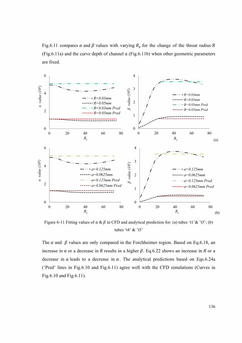
136

Fig.6.11 compares and values with varying for the change of the throat radius

(Fig.6.11a) and the curve depth of channel (Fig.6.11b) when other geometric parameters

are fixed.

(a)

(b)

Figure 6-11 Fitting values of & in CFD and analytical prediction for: (a) tubes ‘t1’& ’t5’; (b)

tubes ‘t4’ & ’t5’

The and values are only compared in the Forchheimer region. Based on Eq.6.18, an

increase in or a decrease in results in a higher . Eq.6.22 shows an increase in or a

decrease in leads to a decrease in . The analytical predictions based on Eqs.6.24a

(‘Pred’ lines in Fig.6.10 and Fig.6.11) agree well with the CFD simulations (Curves in

Fig.6.10 and Fig.6.11).

0

2

4

6

0 20 40 60 80

αva

lue

(104 )

Re

R=0.03mmR=0.05mmR=0.03mm PredR=0.05mm Pred

0

1

2

3

4

0 20 40 60 80β

valu

e (1

05 )

Re

R=0.03mm

R=0.05mm

R=0.03mm Pred

R=0.05mm Pred

0

2

4

6

0 20 40 60 80

αva

lue

(104 )

Re

a=0.125mma=0.0625mma=0.125mm Preda=0.0625mm Pred

0

1

2

3

4

0 20 40 60 80

βva

lue

(105 )

Re

a=0.125mm

a=0.0625mm

a=0.125mm Pred

a=0.0625mm Pred

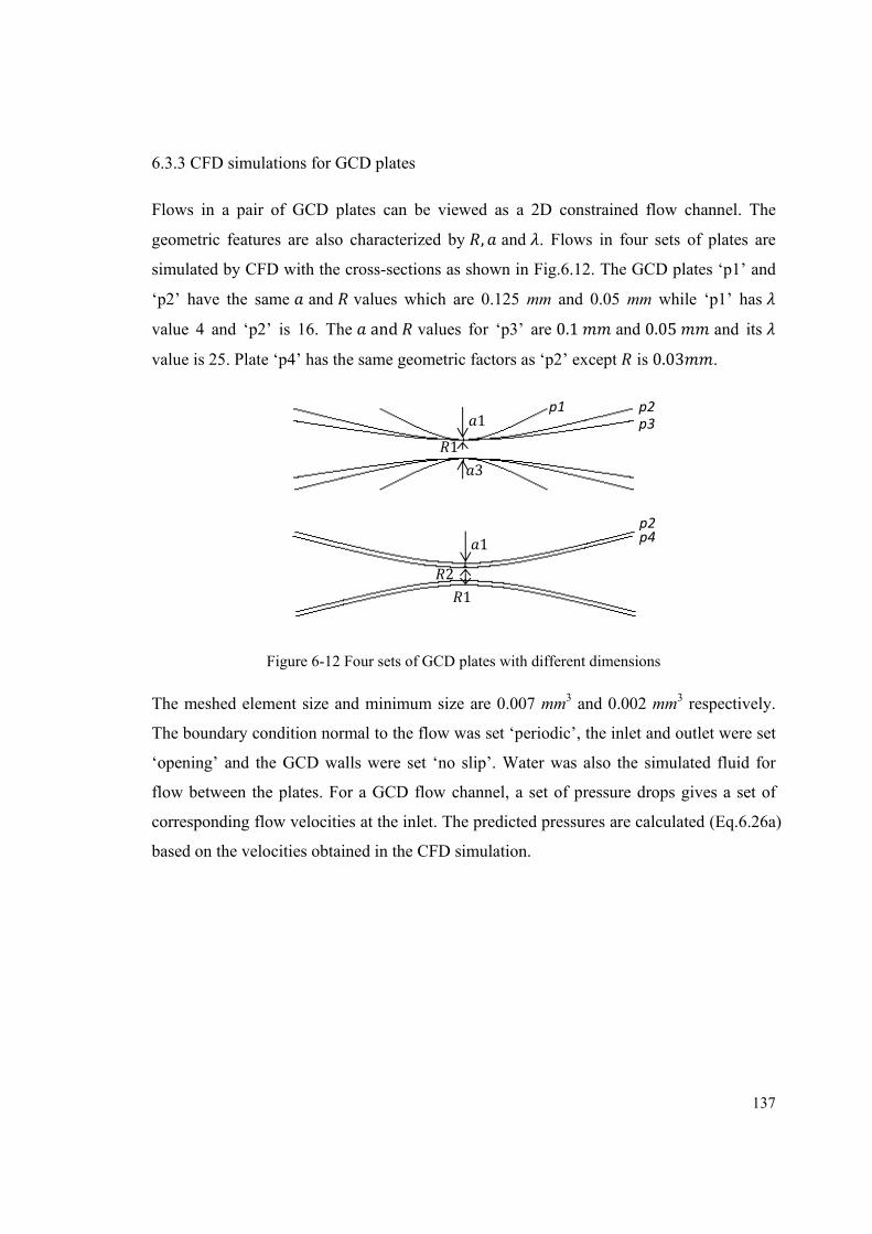
137

6.3.3 CFD simulations for GCD plates

Flows in a pair of GCD plates can be viewed as a 2D constrained flow channel. The

geometric features are also characterized by , and . Flows in four sets of plates are

simulated by CFD with the cross-sections as shown in Fig.6.12. The GCD plates ‘p1’ and

‘p2’ have the same and values which are 0.125 mm and 0.05 mm while ‘p1’ has

value 4 and ‘p2’ is 16. The and values for ‘p3’ are 0.1 and 0.05 and its

value is 25. Plate ‘p4’ has the same geometric factors as ‘p2’ except is 0.03 .

Figure 6-12 Four sets of GCD plates with different dimensions

The meshed element size and minimum size are 0.007 mm3 and 0.002 mm3 respectively.

The boundary condition normal to the flow was set ‘periodic’, the inlet and outlet were set

‘opening’ and the GCD walls were set ‘no slip’. Water was also the simulated fluid for

flow between the plates. For a GCD flow channel, a set of pressure drops gives a set of

corresponding flow velocities at the inlet. The predicted pressures are calculated (Eq.6.26a)

based on the velocities obtained in the CFD simulation.

131 p1 p2

p3

12 1 p2 p4

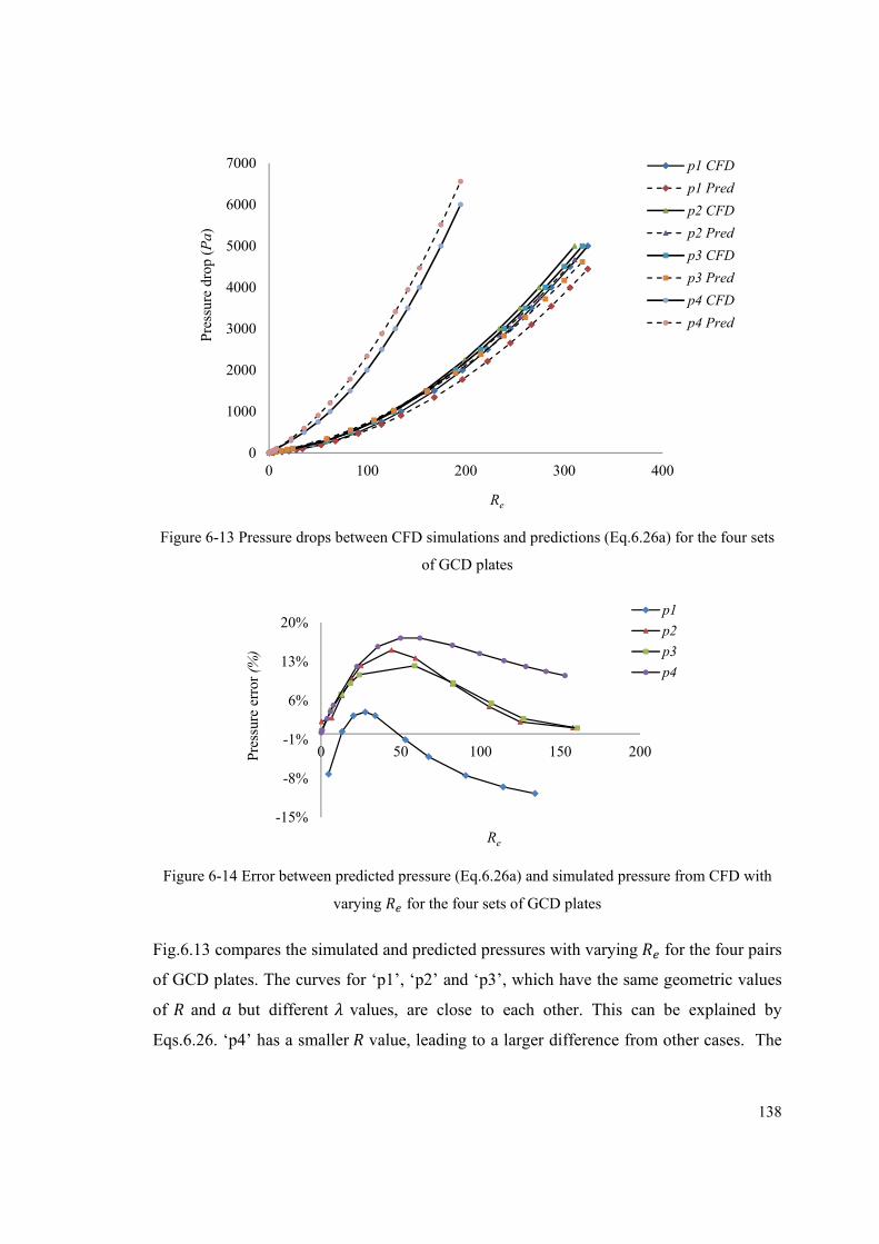
138

Figure 6-13 Pressure drops between CFD simulations and predictions (Eq.6.26a) for the four sets

of GCD plates

Figure 6-14 Error between predicted pressure (Eq.6.26a) and simulated pressure from CFD with

varying for the four sets of GCD plates

Fig.6.13 compares the simulated and predicted pressures with varying for the four pairs

of GCD plates. The curves for ‘p1’, ‘p2’ and ‘p3’, which have the same geometric values

of and but different values, are close to each other. This can be explained by

Eqs.6.26. ‘p4’ has a smaller value, leading to a larger difference from other cases. The

0

1000

2000

3000

4000

5000

6000

7000

0 100 200 300 400

Pre

ssur

e dr

op (

Pa)

Re

p1 CFD

p1 Pred

p2 CFD

p2 Pred

p3 CFD

p3 Pred

p4 CFD

p4 Pred

-15%

-8%

-1%

6%

13%

20%

0 50 100 150 200Pres

sure

err

or (

%)

Re

p1

p2

p3

p4

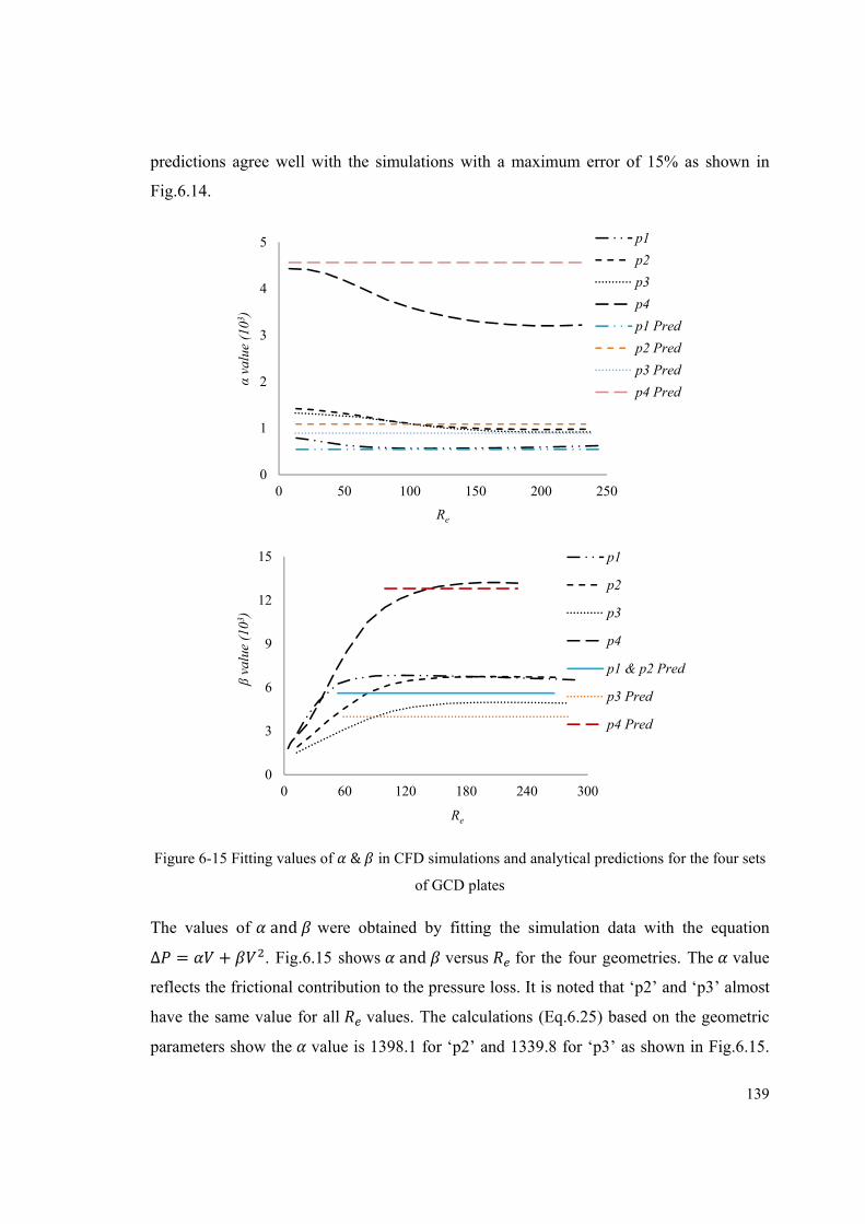
139

predictions agree well with the simulations with a maximum error of 15% as shown in

Fig.6.14.

Figure 6-15 Fitting values of & in CFD simulations and analytical predictions for the four sets

of GCD plates

The values of and were obtained by fitting the simulation data with the equation ∆ = + . Fig.6.15 shows and versus for the four geometries. The value

reflects the frictional contribution to the pressure loss. It is noted that ‘p2’ and ‘p3’ almost

have the same value for all values. The calculations (Eq.6.25) based on the geometric

parameters show the value is 1398.1 for ‘p2’ and 1339.8 for ‘p3’ as shown in Fig.6.15.

0

1

2

3

4

5

0 50 100 150 200 250

αva

lue

(103 )

Re

p1

p2

p3

p4

p1 Pred

p2 Pred

p3 Pred

p4 Pred

0

3

6

9

12

15

0 60 120 180 240 300

βva

lue

(103 )

Re

p1

p2

p3

p4

p1 & p2 Pred

p3 Pred

p4 Pred

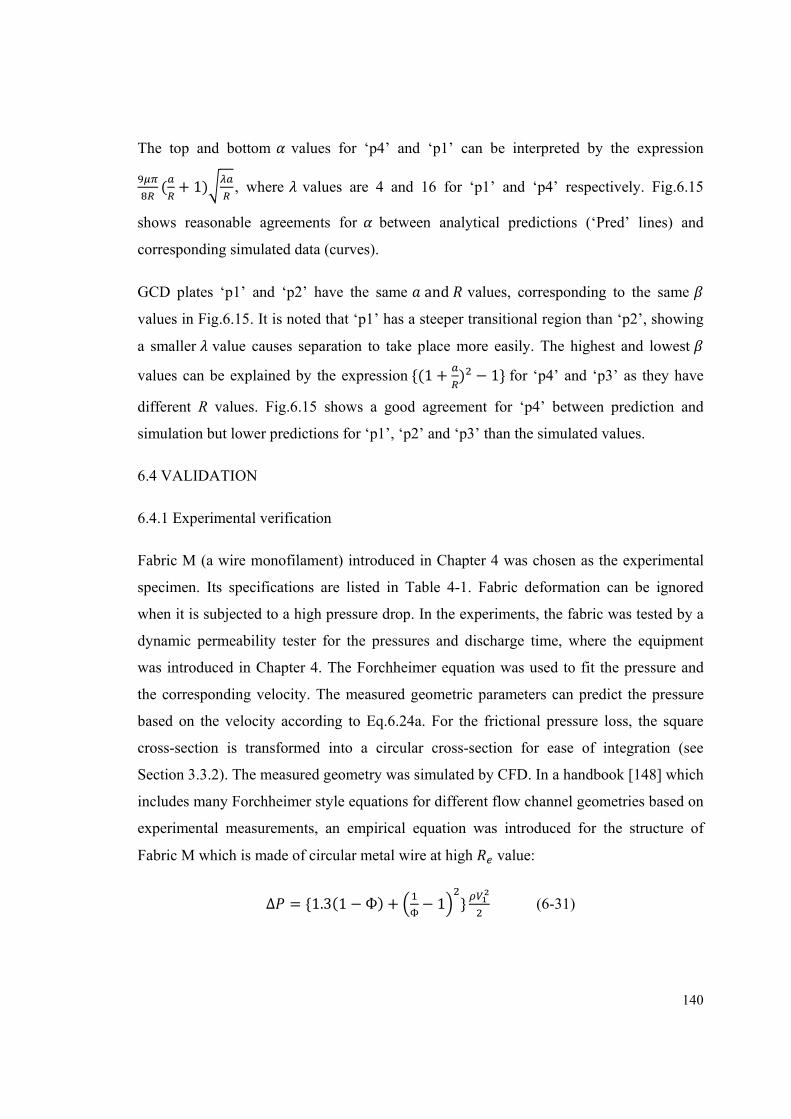
140

The top and bottom values for ‘p4’ and ‘p1’ can be interpreted by the expression ( + 1) , where values are 4 and 16 for ‘p1’ and ‘p4’ respectively. Fig.6.15

shows reasonable agreements for between analytical predictions (‘Pred’ lines) and

corresponding simulated data (curves).

GCD plates ‘p1’ and ‘p2’ have the same and values, corresponding to the same

values in Fig.6.15. It is noted that ‘p1’ has a steeper transitional region than ‘p2’, showing

a smaller value causes separation to take place more easily. The highest and lowest

values can be explained by the expression {(1 + ) − 1} for ‘p4’ and ‘p3’ as they have

different R values. Fig.6.15 shows a good agreement for ‘p4’ between prediction and

simulation but lower predictions for ‘p1’, ‘p2’ and ‘p3’ than the simulated values.

6.4 VALIDATION

6.4.1 Experimental verification

Fabric M (a wire monofilament) introduced in Chapter 4 was chosen as the experimental

specimen. Its specifications are listed in Table 4-1. Fabric deformation can be ignored

when it is subjected to a high pressure drop. In the experiments, the fabric was tested by a

dynamic permeability tester for the pressures and discharge time, where the equipment

was introduced in Chapter 4. The Forchheimer equation was used to fit the pressure and

the corresponding velocity. The measured geometric parameters can predict the pressure

based on the velocity according to Eq.6.24a. For the frictional pressure loss, the square

cross-section is transformed into a circular cross-section for ease of integration (see

Section 3.3.2). The measured geometry was simulated by CFD. In a handbook [148] which

includes many Forchheimer style equations for different flow channel geometries based on

experimental measurements, an empirical equation was introduced for the structure of

Fabric M which is made of circular metal wire at high value:

∆ = {1.3(1 − Ф) + Ф − 1 } (6-31)

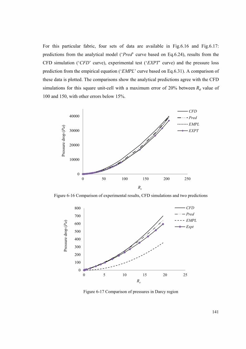
141

For this particular fabric, four sets of data are available in Fig.6.16 and Fig.6.17:

predictions from the analytical model (‘Pred’ curve based on Eq.6.24), results from the

CFD simulation (‘CFD’ curve), experimental test (‘EXPT’ curve) and the pressure loss

prediction from the empirical equation (‘EMPL’ curve based on Eq.6.31). A comparison of

these data is plotted. The comparisons show the analytical predictions agree with the CFD

simulations for this square unit-cell with a maximum error of 20% between value of

100 and 150, with other errors below 15%.

Figure 6-16 Comparison of experimental results, CFD simulations and two predictions

Figure 6-17 Comparison of pressures in Darcy region

0

10000

20000

30000

40000

0 50 100 150 200 250

Pre

ssur

e dr

op (

Pa)

Re

CFD

Pred

EMPL

EXPT

0

100

200

300

400

500

600

700

800

0 5 10 15 20 25

Pre

ssur

e dr

op (

Pa)

Re

CFD

Pred

EMPL

Expt

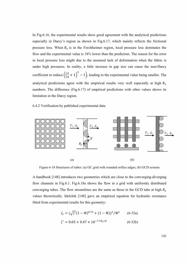
142

In Fig.6.16, the experimental results show good agreement with the analytical predictions

especially in Darcy’s region as shown in Fig.6.17, which mainly reflects the frictional

pressure loss. When is in the Forchheimer region, local pressure loss dominates the

flow and the experimental value is 18% lower than the prediction. The reason for the error

in local pressure loss might due to the assumed lack of deformation when the fabric is

under high pressures. In reality, a little increase in gap size can cause the non-Darcy

coefficient to reduce + 1 − 1 , leading to the experimental value being smaller. The

analytical predictions agree with the empirical results very well especially at high

numbers. The difference (Fig.6.17) of empirical predictions with other values shows its

limitation in the Darcy region.

6.4.2 Verification by published experimental data

(a) (b)

Figure 6-18 Structures of tubes: (a) GC grid with rounded orifice edges; (b) GCD screens

A handbook [148] introduces two geometries which are close to the converging-diverging

flow channels in Fig.6.1. Fig.6.18a shows the flow in a grid with uniformly distributed

converging tubes. The flow streamlines are the same as those in the GCD tube at high

values theoretically. Idelchik [148] gave an empirical equation for hydraulic resistance

fitted from experimental results for this geometry:

= ( (1 − Ф) . + (1 − Ф)) Ф⁄ (6-32a) = 0.03 + 0.47 × 10 . / (6-32b)

V2, A2 V1, A1

V2, A2 V1, A1

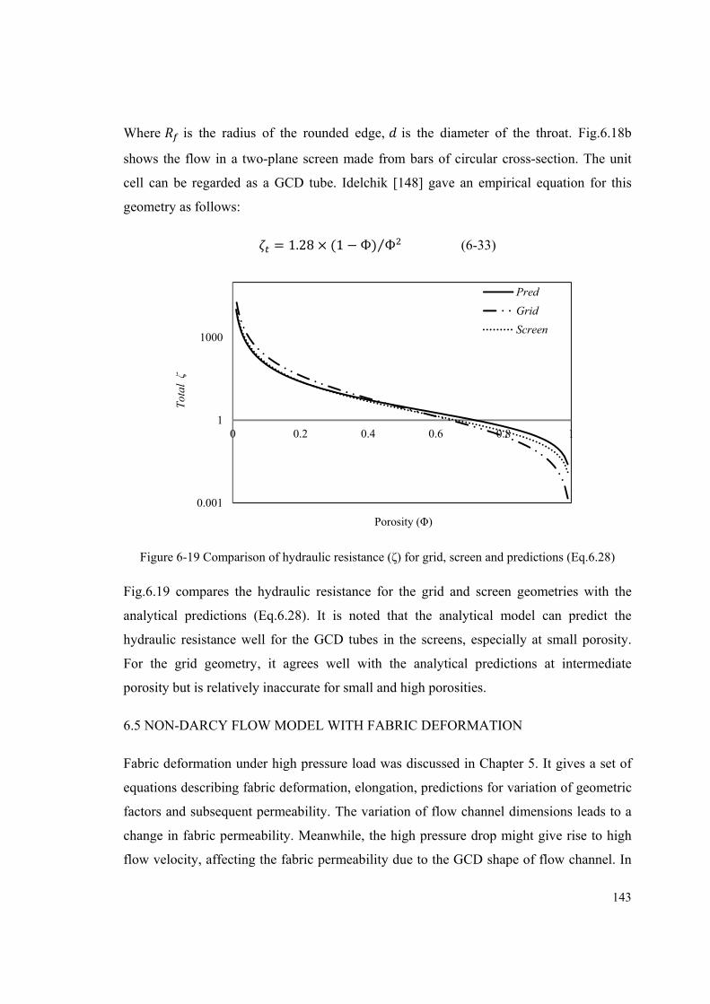
143

Where is the radius of the rounded edge, is the diameter of the throat. Fig.6.18b

shows the flow in a two-plane screen made from bars of circular cross-section. The unit

cell can be regarded as a GCD tube. Idelchik [148] gave an empirical equation for this

geometry as follows: = 1.28 × (1 − Ф) Ф⁄ (6-33)

Figure 6-19 Comparison of hydraulic resistance (ζ) for grid, screen and predictions (Eq.6.28)

Fig.6.19 compares the hydraulic resistance for the grid and screen geometries with the

analytical predictions (Eq.6.28). It is noted that the analytical model can predict the

hydraulic resistance well for the GCD tubes in the screens, especially at small porosity.

For the grid geometry, it agrees well with the analytical predictions at intermediate

porosity but is relatively inaccurate for small and high porosities.

6.5 NON-DARCY FLOW MODEL WITH FABRIC DEFORMATION

Fabric deformation under high pressure load was discussed in Chapter 5. It gives a set of

equations describing fabric deformation, elongation, predictions for variation of geometric

factors and subsequent permeability. The variation of flow channel dimensions leads to a

change in fabric permeability. Meanwhile, the high pressure drop might give rise to high

flow velocity, affecting the fabric permeability due to the GCD shape of flow channel. In

0.001

1

1000

0 0.2 0.4 0.6 0.8 1

Tot

al ζ

Porosity (Φ)

Pred

Grid

Screen

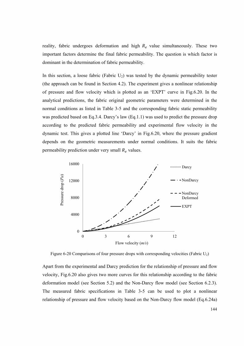
144

reality, fabric undergoes deformation and high value simultaneously. These two

important factors determine the final fabric permeability. The question is which factor is

dominant in the determination of fabric permeability.

In this section, a loose fabric (Fabric U2) was tested by the dynamic permeability tester

(the approach can be found in Section 4.2). The experiment gives a nonlinear relationship

of pressure and flow velocity which is plotted as an ‘EXPT’ curve in Fig.6.20. In the

analytical predictions, the fabric original geometric parameters were determined in the

normal conditions as listed in Table 3-5 and the corresponding fabric static permeability

was predicted based on Eq.3.4. Darcy’s law (Eq.1.1) was used to predict the pressure drop

according to the predicted fabric permeability and experimental flow velocity in the

dynamic test. This gives a plotted line ‘Darcy’ in Fig.6.20, where the pressure gradient

depends on the geometric measurements under normal conditions. It suits the fabric

permeability prediction under very small values.

Figure 6-20 Comparisons of four pressure drops with corresponding velocities (Fabric U2)

Apart from the experimental and Darcy prediction for the relationship of pressure and flow

velocity, Fig.6.20 also gives two more curves for this relationship according to the fabric

deformation model (see Section 5.2) and the Non-Darcy flow model (see Section 6.2.3).

The measured fabric specifications in Table 3-5 can be used to plot a nonlinear

relationship of pressure and flow velocity based on the Non-Darcy flow model (Eq.6.24a)

0

4000

8000

12000

16000

0 3 6 9 12

Pre

ssur

e dr

op (

Pa)

Flow velocity (m/s)

Darcy

NonDarcy

NonDarcyDeformed

EXPT

145

with no deformation concerned, the prediction is shown as the ‘NonDarcy’ curve in

Fig.6.20. The deformation model (Eq.5.14) predicts new geometric parameters under high

pressure load. Considering the fabric deformation, the Forchheimer equation with the new

geometric parameters (Eqs.5.15, 5.16, 5.25-27) can predict a new nonlinear relationship as

shown by the ‘NonDarcy Deformed’ curve in Fig.6.20, which is close to the experimental

measurements as shown by the ‘EXPT’ curve in Fig.6.20. Fig.6.20 indicates the Non-

Darcy flow model differs with the Darcy flow model significantly when the value

reaches the Forchheimer region (‘C’ in Fig.6.6). The difference increases as the flow

velocity is increasing. The Non-Darcy flow model only applies for a ‘rigid’ woven fabric

where deformation can be ignored under high pressure load, as shown by accurate

prediction in Fig.6.16. However, as to an easily-deformed fabric such as U2, the

deformation model plays a vital role in predicting the fabric permeability as the gap

geometry has been changed by the pressure load. The gap radius is increased, and the yarn

shape factor and fabric thickness are changed by the deformation. For an increased gap

size, the pressure required is smaller than the original value for the same flow velocity.

Therefore, considering these factors, the deformation model draws the Non-Darcy flow

prediction much closer to the experimental results as shown in Fig.6.20.

6.6 CONCLUSIONS

When a Newtonian fluid flows in a gradual converging-diverging channel, the curved

inner surface diverts the flow. The channel is filled with fluid flow when value is less

than a critical value. The flow equation is derived from the integration of the application of

parabolic stream profiles in Poiseuille straight flow. The flow equation shows a linear

relationship of pressure and flow velocity. When is increased, separation is observed

from CFD simulation from the curved expansion wall. The convective acceleration should

not be ignored in this case. The integration of Navier-Stokes equation shows the total

pressure loss in the channel contains a linear velocity term (Darcy term) and velocity

square term (non-Darcy term). Two pressure losses can be predicted based on the velocity

at the channel inlet. The pressure loss consists of Darcy (frictional) and non-Darcy (local)

parts. The former is a function of the channel geometry and fluid property while the latter

146

is derived from continuity theory and the Bernoulli equation, which depends on the

channel geometry solely.

The analytical model was validated by CFD simulations. The relationship of pressure and

flow velocity was fitted by the Forchheimer equation, showing three regions (Darcy,

transitional and Forchheimer regions) as increases. Five GCD tubes were simulated and

compared with the analytical predictions (Eq.6.24), showing good agreement. A sharper

curved channel would have a smaller critical number for the separation or transitional

region, resulting in poorer agreement with the predictions. A sensitivity study showed an

increase of throat radius or a decrease of curved depth would both obtain lower Darcy and

non-Darcy coefficients. Four GCD plates were also simulated and compared with the

analytical predictions (Eq.6.26), showing good agreement with each other with maximum

difference of 15%. The geometry had the same effect on the hydraulic resistance with

GCD tubes. Experimental verification on a wire monofilament woven fabric showed it

agreed with the prediction within 20% error. Published experimental data showed good

agreement with the predictions. Comparisons of hydraulic resistance against porosity for

gradual converging grids and gradual converging-diverging screens showed the

predictions agreed with the screens very well while good agreement with the grid was only

obtained around intermediate porosities.

The Darcy flow model shows a linear relationship of pressure and flow velocity. It fits the

static permeability behaviour when flow is at low . The Non-Darcy flow model is based

on the Darcy model by adding a Non-Darcy term, which is evident at high . This model

applies for a high stiffness porous medium where the deformation can be ignored. A real

fabric has evident deformation when it is subjected to a high pressure drop, which changes

its flow channel dimensions. The deformation model can account for the effect of pressure

on fabric deformation, predicting the real permeability under high pressure drop. This

modifies the non-Darcy flow model so that it is much closer to the real fabric permeability.

147

CHAPTER 7

CONCLUSIONS AND FUTURE WORK

7.1 INTRODUCTION

An interesting topic was proposed based on the experimental results of fabric through-

thickness permeability in Chapter 3, which is about analytical modeling of woven fabric

permeability in specific applications, such as airbags for body protection. After the

literature review, it was found gaps between yarns and within the yarns in a woven fabric

have different fluid flow theories to model their permeabilities. The gap flow can be

regarded as fluid flow through a gradual converging-diverging (GCD) flow channel while

the yarn flow is simplified as a combination of fluid flow along and perpendicular to

unidirectional fibres. The fabric permeability is a function of gap permeability and yarn

permeability (Eq.3.4), which also depends on the flow state in terms of value.

As is known, airbag fabric undergoes high pressure load in its inflation. This gives rise to a

deformation to its geometry and structure, resulting in a change in permeability.

Meanwhile, the high pressure drop may lead to a nonlinear relationship of pressure and

flow velocity in the gap channel, nonetheless the flow is laminar. Therefore, in this thesis,

fabric dynamic permeability was investigated experimentally. Also deformation modeling

of one-layer of woven fabric under high pressure load and nonlinear flow through fabric

gaps at high values are extensions to the investigation of the fabric dynamic

permeability. Moreover, the developed models were verified for their accuracy by

simulation and experiment.

This chapter summaries the developed models in the previous chapters, including their

verification as well as their limitations. A number of suggestions for future work based on

the work in this thesis are recommended in the final section.

7.2 GENERAL SUMMARY AND CONCLUSIONS

(1) Static gap permeability ( . 3.4):

148

The Newtonian fluid considered in the model is assumed to be incompressible with

constant viscosity and density due to low flow rates; the flow is laminar and the flow

process is steady state; the flow inertial terms and yarn motion are neglected; the flow

velocity at the surface and inside of the yarns is assumed to be zero while at the centre-line

of the channel it is maximum; fluid flow is considered in the direction perpendicular to the

fabric, the transverse component of the velocity is negligible because the highest pressure

gradient is near the narrowest region where the flow is almost parallel to the channel

surface.

A circular cross-section of flow channel is transformed from the rectangular cross-section

as a unit cell in a woven fabric by defining the hydraulic diameter. Four geometric

parameters were used in deriving the analytical model: throat radius, half yarn width,

fabric thickness and curvature of the flow channel. A parabolic equation is used to

describe the GCD channel. Substitution of its radius into the Hagen-Poiseuille equation

gives an expression relating pressure and flow rate (Eq.3.17). A permeability equation

based on the four fabric geometric parameters is obtained by integrating and simplifying

the formula, in which the four parameters are gap size, yarn width, yarn shape factor and

fabric thickness.

The gap permeability prediction was verified by CFD simulation and experiment. GCD

flow channels were generated in TexGen and meshed in HyperMesh. Flow behaviour was

simulated by CFD. The simulated permeability agreed with the corresponding prediction

well. Nine one-layer loose woven fabrics were tested for their geometric parameters. Their

permeabilities were measured by an air permeability tester. The comparisons showed the

analytical model (Eq.3.4) gave good predictions against experimental permeabilities

within 35% error for all fabrics. However, the Kulichenko model [27], which assumed

fabric gaps as a set of straight tubes, gave errors of over 70% in permeability prediction.

(2) Static yarn permeability ( . 3.4):

Combination of the Gebart and Advani models can predict permeability of a crimped yarn

in a woven fabric in terms of the crimp angle, fibre radius, fibre arrangement and volume

fraction. Three fibre arrays (different and values) were simulated for the axial and

149

transverse permeabilities by CFD. Comparisons of predictions and simulations showed the

transverse model can predict permeability well with a maximum error of 20%. The axial

model agrees with the simulation accurately at high values. Two airbag fabrics with

high were tested for their permeabilities in experiments. A comparison of the tested

permeability and analytical prediction (Eq.3.10) showed agreement with errors of less than

20%.

(3) Static permeability of woven fabrics ( ):

Based on the gap ( ) and yarn ( ) permeabilities, a unified model for one-layer of

woven fabric ( ) permeability was proposed in terms of porosity (Φ): = Ф +(1 − Ф) . Calculations (Table 3-7) showed gap permeability dominates the fabric

permeability for loose fabrics.

A through-thickness permeability model for 3D woven fabric was derived based on the

permeability of each fabric layer. Four 3D woven fabrics were measured for the

permeability. The predictions showed good agreements with the experimental data. A

sensitivity study showed that the most important contribution to the 3D fabric permeability

was the gap permeability.

(4) Dynamic permeability of woven fabrics:

An air discharging tester was employed to obtain fabric dynamic permeability. The

pressure history was recorded by transducers inside the tester. The operating principle was

to expel the discharged gas at high pressure through the fabric into a chamber at

atmospheric pressure. The pressure and velocity are fitted by the Forchheimer equation,

with the fabric dynamic permeability acquired from the first order velocity coefficient.

The high pressure causes fabric structural deformation, unlike the static test at a constant

low pressure. Three fabrics were measured for their dynamic permeability: a loose metal

fabric, a loose cotton fabric and a tight nylon fabric. The metal fabric was assumed to be

without deformation under high pressure. The experimental data showed a slight

difference between static and dynamic permeabilities. The loose and tight fabrics were

150

stretched under high pressure load. The dynamic permeability for loose fabric was higher

while for tight fabric was lower than their static permeabilities.

(5) Fabric deformation model:

Airbag fabric is subjected to high pressure load when the airbag is inflated, leading to

fabric deformation. A device was designed to imitate the deformation behaviour under

high pressure. It utilized a vacuum pump to apply pressure to the fabric which was

clamped at one side of it. The vacuum pump can supply different pressure drops, leading

to different levels of fabric deformation. Two geometric parameters were tested manually

in the experiment: the maximum displacement and the deflected profile across a diameter

under the pressure load.

Two trigonometric approximations (Eq.5.2) were assumed for the displacements involving

two unknown coefficients. All derivations were conducted in polar coordinates for the

circular fabric samples. Based on the large deflection plate theory, strain energy, bending

energy and work done were added to calculate the total energy of the system, from which

the deflection function was obtained by substitution of the differentiated approximations

(Eq.5.10) into the total energy and minimizing it. Two expressions for displacement and

deflected profile were developed involving pressure load, fabric dimensions and fabric

mechanical properties.

A tight and a loose fabric were analysed for their deformations under high pressure load.

The analytical predictions agreed with the experimental measurements well for both

maximum displacements and deflected profiles. A sensitivity study showed the fabric

deformation was affected by sample radius and thickness, fabric Young’s modulus and

Poisson’s ratio as expected.

(6) Deformed fabric permeability:

An analytical model was proposed for predicting the through-thickness permeability of

woven fabric under high pressure load. The model was based on the accuracy of the static

permeability and the fabric deflection predictions. Fabric deflection causes the yarn fibre

volume fraction and the crimp angle to increase, leading to a decrease of tight fabric

151

permeability. In contrast, the deflection causes the gap radius to increase, resulting in an

increase of loose fabric permeability. The permeability predictions agreed well with the

experimental data. A sensitivity study showed the critical porosity and fabric thickness for

fabric permeability to increase or decrease with an increase of pressure. An increase of

fabric Young’s modulus or a decrease of fabric radius would cause the tight fabric

permeability to increase and the loose fabric permeability to decrease when the fabric is

under the same pressure.

(7) Non-Darcy flow behaviour:

When a Newtonian fluid flows in a GCD channel, the curved wall diverts the streamlines.

Flow for the GCD channel follows the profile of the channel for small values. A linear

relationship of pressure and flow velocity was obtained from the curved flow equation.

When gets higher, separation of flow from the diverging wall occurs, giving the flow a

convective acceleration.

The Navier-Stokes equation shows the pressure loss in the flow channel contains a linear

velocity term (Darcy term) and a velocity squared term (Non-Darcy term). For GCD

channels, the pressure loss was predicted based on the inlet velocity in the channel. The

Darcy term is a function of the channel geometry and fluid viscosity; the Non-Darcy term

is derived from continuity theory and the ideal Bernoulli equation, which depends on the

channel geometry completely.

The developed Darcy and Non-Darcy terms were verified by CFD simulation. Five GCD

tubes and four sets of GCD plates were generated and meshed. CFD simulations showed

that pressure versus inlet velocity exhibited three regions with : Darcy, transitional and

Forchheimer regions. The simulated results showed good agreement with the

corresponding predictions. However, a sharper flow throat would have a smaller value

for the transitional region and poorer agreement with the prediction. An increase of the

throat radius ( ) or a decrease of the curved depth ( ) of wall would result in lower Darcy

and Non-Darcy coefficients.

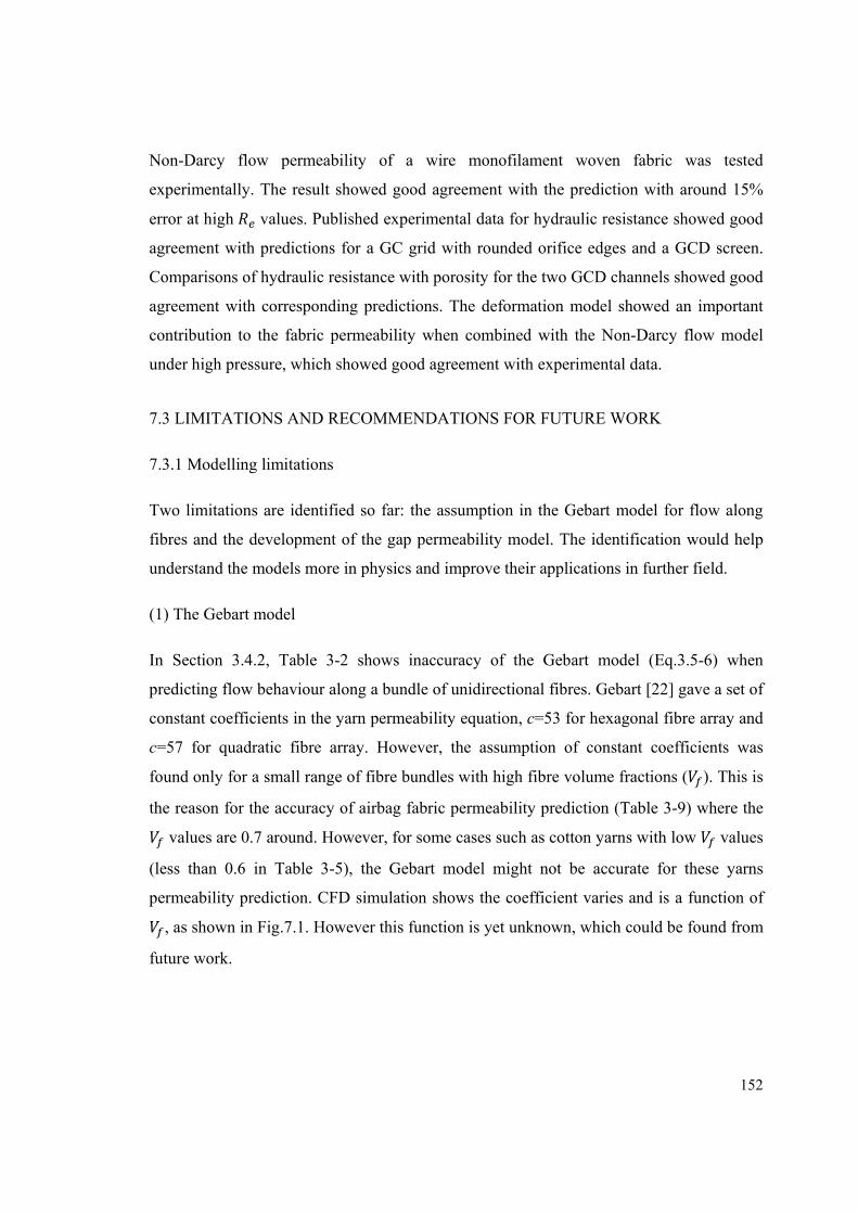
152

Non-Darcy flow permeability of a wire monofilament woven fabric was tested

experimentally. The result showed good agreement with the prediction with around 15%

error at high values. Published experimental data for hydraulic resistance showed good

agreement with predictions for a GC grid with rounded orifice edges and a GCD screen.

Comparisons of hydraulic resistance with porosity for the two GCD channels showed good

agreement with corresponding predictions. The deformation model showed an important

contribution to the fabric permeability when combined with the Non-Darcy flow model

under high pressure, which showed good agreement with experimental data.

7.3 LIMITATIONS AND RECOMMENDATIONS FOR FUTURE WORK

7.3.1 Modelling limitations

Two limitations are identified so far: the assumption in the Gebart model for flow along

fibres and the development of the gap permeability model. The identification would help

understand the models more in physics and improve their applications in further field.

(1) The Gebart model

In Section 3.4.2, Table 3-2 shows inaccuracy of the Gebart model (Eq.3.5-6) when

predicting flow behaviour along a bundle of unidirectional fibres. Gebart [22] gave a set of

constant coefficients in the yarn permeability equation, c=53 for hexagonal fibre array and

c=57 for quadratic fibre array. However, the assumption of constant coefficients was

found only for a small range of fibre bundles with high fibre volume fractions ( ). This is

the reason for the accuracy of airbag fabric permeability prediction (Table 3-9) where the

values are 0.7 around. However, for some cases such as cotton yarns with low values

(less than 0.6 in Table 3-5), the Gebart model might not be accurate for these yarns

permeability prediction. CFD simulation shows the coefficient varies and is a function of

, as shown in Fig.7.1. However this function is yet unknown, which could be found from

future work.

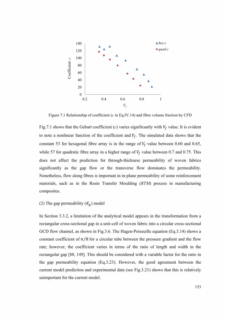
153

Figure 7.1 Relationship of coefficient (c in Eq.IV.14) and fibre volume fraction by CFD

Fig.7.1 shows that the Gebart coefficient (c) varies significantly with value. It is evident

to note a nonlinear function of the coefficient and . The simulated data shows that the

constant 53 for hexagonal fibre array is in the range of value between 0.60 and 0.65,

while 57 for quadratic fibre array in a higher range of value between 0.7 and 0.75. This

does not affect the prediction for through-thickness permeability of woven fabrics

significantly as the gap flow or the transverse flow dominates the permeability.

Nonetheless, flow along fibres is important in in-plane permeability of some reinforcement

materials, such as in the Resin Transfer Moulding (RTM) process in manufacturing

composites.

(2) The gap permeability ( ) model

In Section 3.3.2, a limitation of the analytical model appears in the transformation from a

rectangular cross-sectional gap in a unit-cell of woven fabric into a circular cross-sectional

GCD flow channel, as shown in Fig.3.6. The Hagen-Poiseuille equation (Eq.3.14) shows a

constant coefficient of 8⁄ for a circular tube between the pressure gradient and the flow

rate; however, the coefficient varies in terms of the ratio of length and width in the

rectangular gap [88, 149]. This should be considered with a variable factor for the ratio in

the gap permeability equation (Eq.3.23). However, the good agreement between the

current model prediction and experimental data (see Fig.3.21) shows that this is relatively

unimportant for the current model.

0

20

40

60

80

100

120

140

0.2 0.4 0.6 0.8 1

Coe

ffic

ient

c

Vf

hex c

quad c

154

(a) (b)

Figure 7.2 (a) Current GCD flow channel, (b) theoretical GCD flow channel

Another limitation in the development of the model is the application of hydraulic

diameter, which simplified the integration significantly. Nonetheless, it should be pointed

out that the transformation from rectangular gap to circular gap by the definition of

hydraulic diameter at the throat (‘R’ in Fig.7.2) might not be reasonable along the flow

direction, as a GCD flow channel formed by one hydraulic diameter in addition to a

measured yarn shape factor is not physically correct. However all transformations along

the yarn height to hydraulic diameter (arbitrary position ‘r’ in Fig.7.2) mean that a

different flow channel developed from accurate measurements of yarn width, yarn height

and yarn shape factor as shown in Fig.7.2b. Although this is more reasonable and

convincing, it is evident that this would require more work in the measurements and

transformations (Eq.3.19) and would not be as simple as the current model.

7.3.2 Recommendations for future work

Apart from the limitations in Section 7.3.1, the following points will in general improve

the work in future.

• Static gap permeability ( ):

An analytical gap permeability model could be developed for flow in a rectangular

cross-sectional GCD gap. This can avoid the variable factor mentioned in the first

paragraph in Section 7.3.1(2). Some work has been done which can be found in

Appendix VII. Recommended future work for this model is to compare its prediction

with the current model (Eq.3.23) as well as experimental data.

Flow

R r

Flow

R r

155

• Static yarn permeability ( ):

Although a device is attractive to investigate flow behaviour transverse to or along

yarns experimentally, the yarn twist and interwoven structure make this difficult. In

simulation, TexGen cannot create a yarn containing fibres like a real yarn structure at

the moment. However, numerical simulation is a promising method to simulate flow

behaviour in yarns, which is recommended as a future work.

• Dynamic permeability investigation:

To predict fabric dynamic permeability accurately, fabric geometric dimensions should

be measured during air discharge. A digital video camera with a microscope attachment

is recommended mounted on the dynamic permeability tester (Fig.4.1). This will give

exact dimensions of fabric during the dynamic test, such as fabric deflection and unit-

cell size under high pressure.

• Fabric deformation model:

(1) Poisson’s ratio should be measured for woven fabrics in weft and warp directions.

(2) Mesoscale (unit-cell) level fabric deformation under pressure load should be

characterised, where shear, stretch and compression are considered respectively.

(3) Fabric deformation should be modelled considering an anisotropic material

analytically under high pressure load.

• Non-Darcy flow model:

(1) The reason for the maximum difference between prediction and simulation in the

transitional region as shown in Fig.6.9 and Fig.6.14 should be studied.

(2) The Non-Darcy flow model should be extended to other geometry applications,

such as flow with high value in yarns, nozzles and diffusers.

156

REFERENCES

1. Lego-Airbag, [cited 26/10/2012]: http://blog.electricbricks.com/en/2010/11/lego-airbag/.

2. Mei, C. C., Vernescu, B. and Ebrary, I., Homogenization methods for multiscale mechanics [electronic resource] 2010: Singapore; London; World Scientific. 330.

3. TexGen. [cited 22/11/2011]: http://texgen.sourceforge.net/index.php/Main_Page.

4. Henry, P. S. H., Diffusion in absorbing media. Proceedings of the Royal Society of London Series a-Mathematical, Physical & Engineering Sciences, 1939. 171: p. 215-241.

5. Chen, B. X. and Chou, T. W., Compaction of woven-fabric preforms in liquid composite molding processes: single-layer deformation. Composites Science and Technology, 1999. 59(10): p. 1519-1526.

6. Julian, A. W., Falls among the elderly—Human and environmental factors. Accident Analysis & Prevention, 1978. 10(1): p. 21-33.

7. Tamura, T., Yoshimura, T., Sekine, M., Uchida, M. and Tanaka, O., A wearable airbag to prevent fall injuries. Ieee Transactions on Information Technology in Biomedicine, 2009. 13(6): p. 910-914.

8. Kovacevic, S., Ujevic, D., Schwarz, I., Sajatovic, B. B. and Brnada, S., Analysis of Motor Vehicle Fabrics. Fibres & Textiles in Eastern Europe, 2008. 16(6): p. 32-38.

9. Tutt, B., Sandy, C. and Corliss, J., Status of the development of an airbag landing system for the Orion crew module. in 20th AIAA Aerodynamic decelerator systems technology conference and seminar. 2009. Seattle, Washington, USA.

10. Saldaeva, E., Through thickness air permeability and thermal conductivity analysis for textile materials 2010, PhD thesis, University of Nottingham.

11. Pillai, K. M. and Advani, S. G., Numerical and analytical study to estimate the effect of 2. length scales upon the permeability of a fibrous porous medium. Transport in Porous Media, 1995. 21(1): p. 1-17.

12. Scheidegger, A. E., The physics of flow through porous media. Soil Science, 1958. 86(6): p. 355.

13. Wong, C. C., Modelling the effects of textile preform architecture on permeability, 2006, PhD thesis, The University of Nottingham.

157

14. Das, A. and Ishtiaque, S. M. , Comfort characteristics of fabrics containing twist-less and hollow fibrous assemblies in weft direction. Journal of the Textile Institute, 2004. 3(4): p. 1-7.

15. Senoguz, M. T., Dungan, F. D., Sastry, A. M. and Klamo, J. T., Simulations and experiments on Low-pressure permeation of fabrics:part II-The variable gap model and prediction of permeability. Journal of Composite Materials, 2001. 35(14): p. 1285-1322.

16. Bruschke, M. V. and Advani, S. G., A finite element/control volume approach to mold filling in anisotropic porous media. Polymer Composites, 1990. 11(6): p. 398-405.

17. Xu, P. and Yu, B. M., Developing a new form of permeability and Kozeny–Carman constant for homogeneous porous media by means of fractal geometry. Advances in Water Resources, 2008. 31(1): p. 74-81.

18. Bear, J., Dynamics of fluids in porous media. Environmental science series. 1972, New York,: American Elsevier Pub. Co. xvii, 764 p.

19. Kaviany, M., Principles of heat transfer in porous media (2nd Edition). Mechanical engineering series. 1995, New York: Springer-Verlag. xxii, 708 p.

20. Gutowski, T. G., Morigaki, T. and Cai, Z., The consolidation of laminate composites. Journal of Composite Materials, 1987. 21(2): p. 172-188.

21. Williams, J. G., Morris, C. E. M. and Ennis, B. C., Liquid flow through aligned fiber beds. Polymer Engineering and Science, 1974. 14(6): p. 413-419.

22. Gebart, B. R., Permeability of unidirectional reinforcements for RTM. Journal of Composite Materials, 1992. 26(8): p. 1100-1133.

23. Ngo, N. and Tamma, K. K., Microscale permeability predictions of porous fibrous media. International Journal of Heat and Mass Transfer, 2001. 44(16): p. 3135-3145.

24. Hakanson, J. M., Toll, S. and Lundstrom, T. S., Liquid permeability of an anisotropic fiber web. Textile Research Journal, 2005. 75(4): p. 304-311.

25. Phelan, F. R. and Wise, G., Analysis of transverse flow in aligned fibrous porous media. Composites Part A-Applied Science and Manufacturing, 1996. 27(1): p. 25-34.

26. Smolarkiewicz, P. K. and Winter, C. L., Pores resolving simulation of Darcy flows. Journal of Computational Physics, 2010. 229(9): p. 3121-3133.

27. Kulichenko, A. V., Theoretical analysis, calculation, and prediction of the air permeability of textiles. Fibre Chemistry, 2005. 37(5): p. 371-380.

158

28. Zupin, Z., Hladnik, A. and Dimitrovski, K., Prediction of one-layer woven fabrics air permeability using porosity parameters. Textile Research Journal, 2012. 82(2): p. 117-128.

29. Berdichevsky, A. L. and Cai, Z., Preform permeability predictions by self-consistent method and finite-element simulation. Polymer Composites, 1993. 14(2): p. 132-143.

30. Cai, Z. and Berdichevsky, A. L., An improved self-consistent method for estimating the permeability of a fiber assembly. Polymer Composites, 1993. 14(4): p. 314-323.

31. Bruschke, M. V. and Advani, S. G., Flow of generalized Newtonian fluids across a periodic array of cylinders. Journal of Rheology, 1993. 37(3): p. 479-498.

32. Vander Westhuizen, J. and Du Plessis, J. P., An attempt to quantify fibre bed permeability utilizing the phase average Navier-Stokes equation. Composites Part A-Applied Science and Manufacturing, 1996. 27(4): p. 263-269.

33. Wang, C. Y., Stokes flow through an array of rectangular fibers. International Journal of Multiphase Flow, 1996. 22(1): p. 185-194.

34. Desplentere, F., Lomov, S. V., Woerdeman, D. L., Verpoest, I., Wevers, M. and Bogdanovich, A., Micro-CT characterization of variability in 3D textile architecture. Composites Science and Technology, 2005. 65(13): p. 1920-1930.

35. Badel, P., Vidal-Salle, E., Maire, E. and Boisse, P., Simulation and tomography analysis of textile composite reinforcement deformation at the mesoscopic scale. Composites Science and Technology, 2008. 68(12): p. 2433-2440.

36. Mahadik, Y., Brown, K. A. R. and Hallett, S. R., Characterisation of 3D woven composite internal architecture and effect of compaction. Composites Part A-Applied Science and Manufacturing, 2010. 41(7): p. 872-880.

37. Karahan, M., Lomov, S. V., Bogdanovich, A. E., Mungalov, D. and Verpoest, I., Internal geometry evaluation of non-crimp 3D orthogonal woven carbon fabric composite. Composites Part A-Applied Science and Manufacturing, 2010. 41(9): p. 1301-1311.

38. Endruweit, A. and Long, A. C., Analysis of compressibility and permeability of selected 3D woven reinforcements. Journal of Composite Materials, 2010. 44(24): p. 2833-2862.

39. Mogavero, J. and Advani, S. G., Experimental investigation of flow through multi-layered preforms. Polymer Composites, 1997. 18(5): p. 649-655.

40. Chen, Z. R., Ye, L. and Liu, H. Y., Effective permeabilities of multilayer fabric preforms in liquid composite moulding. Composite Structures. 66(1-4): p. 351-357.

159

41. Song, Y. S., Heider, D. and Youn, J. R., Statistical characteristics of out-of-plane permeability for plain-woven structure. Polymer Composites, 2009. 30(10): p. 1465-1472.

42. Skjetne, E. and Auriault, J. L., New insights on steady, non-linear flow in porous media. European Journal of Mechanics B-Fluids, 1999. 18(1): p. 131-145.

43. Green, L. and Duwez, P., Fluid flow through porous metals. Journal of Applied Mechanics-Transactions of the Asme, 1951. 18(1): p. 39-45.

44. Cornell, D. and Katz, D. L., Flow of gases through consolidated porous media. Industrial and Engineering Chemistry, 1953. 45(10): p. 2145-2152.

45. Firdaouss, M., Guermond, J. L. and LeQuere, P., Nonlinear corrections to Darcy's law at low Reynolds numbers. Journal of Fluid Mechanics, 1997. 343: p. 331-350.

46. Kim, S. M., Numerical investigation on laminar pulsating flow through porous media, 2008, Msc Thesis, Georgia Institute of Technology.

47. Liu, S. J., Afacan, A. and Masliyah, J., Steady incompressible laminar flow in porous media. Chemical Engineering Science, 1994. 49(21): p. 3565-3586.

48. Lee, S. L. and Yang, J. H., Modeling of Darcy-Forchheimer drag for fluid flow across a bank of circular cylinders. International Journal of Heat and Mass Transfer, 1997. 40(13): p. 3149-3155.

49. Ergun, S., Fluid flow through packed columns. Chemical Engineering Progress, 1952. 48(2): p. 89-94.

50. Reynolds, O., On the dynamical theory of incompressible viscous fluids and the determination of the criterion (reprinted from papers on mechanical and physical subjects, vol 2 pg 537-577, 1901). Proceedings of the Royal Society of London Series a-Mathematical and Physical Sciences, 1995. 451(1941): p. 5-47.

51. Adamson, J. E., Application of the Kozeny equation to consolidated porous meida. Nature, 1950. 166(4216): p. 314-315.

52. Blake, F. C., The resistance of packing to fluid flow. Transactions of the American Institute of Chemical Engineers, 1921. 14: p. 415-421.

53. Burke, S. P. and Plummer, W. B., Gas flow through packed columns. Industrial and Engineering Chemistry, 1928. 20(1): p. 1196-1200.

54. Chilton, T. H. and Colburn, A. P., Pressure drop in packed tubes. Industrial and Engineering Chemistry, 1931. 23: p. 913-919.

55. Carman, P. C., Fluid flow through granular beds. Chemical Engineering Research & Design, 1997. 75: p. S32-S48.

160

56. Ergun, S. and Orning, A. A., Fluid flow through randomly packed columns and fluidized beds. Industrial and Engineering Chemistry, 1949. 41(6): p. 1179-1184.

57. Brasquet, C. and Le Cloirec, P., Pressure drop through textile fabrics - experimental data modelling using classical models and neural networks. Chemical Engineering Science, 2000. 55(15): p. 2767-2778.

58. Kyan, C. P., Wasan, D. T. and Kintner, R. C., Flow of single-phase fluids through fibrous beds. Industrial & Engineering Chemistry Fundamentals, 1970. 9(4): p. 596-603.

59. Dullien, F. A. L., Single phase flow through porous media and pore structure. The Chemical Engineering Journal, 1975. 10(1): p. 1-34.

60. Comiti, J. and Renaud, M., A new model for determining mean structure parameters of fixed beds from pressure drop measurements: application to beds packed with parallelepipedal particles. Chemical Engineering Science, 1989. 44(7): p. 1539-1545.

61. Belkacemi, K. and Broadbent, A. D., Air flow through textiles at high differential pressures. Textile Research Journal, 1999. 69(1): p. 52-58.

62. Innocentini, M. D. M., Pardo, A. R. F. and Pandolfelli, V. C., Influence of air compressibility on the permeability evaluation of refractory castables. Journal of the American Ceramic Society, 2000. 83(6): p. 1536-1538.

63. Douglas, J. F., Gasiorek, J. M. and Swaffield, J. A., Fluid mechanics (3rd Edition). 1995, Harlow, Essex, England: First edition published by Pitman, 1979.

64. Whitaker, S., The Forchheimer equation: A theoretical development. Transport in Porous Media, 1996. 25(1): p. 27-61.

65. Chen, Z. X., Lyons, S. L. and Qin, G., Derivation of the Forchheimer law via homogenization. Transport in Porous Media, 2001. 44(2): p. 325-335.

66. Mei, C. C. and Auriault, J. L., The effect of weak inertia on flow through a porous medium. Journal of Fluid Mechanics, 1991. 222: p. 647-663.

67. Wodie, J. C. and Levy, T., Nonlinear rectification of Darcy's law. Comptes Rendus De L Academie Des Sciences Serie Ii, 1991. 312(3): p. 157-161.

68. Burcharth, H. F. and Andersen, O. K., On the one-dimensional steady and unsteady porous flow equations. Coastal Engineering, 1995. 24(3-4): p. 233-257.

69. Skjetne, E. and Auriault, J. L., High-velocity laminar and turbulent flow in porous media. Transport in Porous Media, 1999. 36(2): p. 131-147.

70. Meyer, R. E., A view of the triple deck. SIAM Journal on Applied Mathematics, 1983. 43(4): p. 639-663.

161

71. Smith, F. T., Steday and unsteady boundary layer separation. Annual Review of Fluid Mechanics, 1986. 18: p. 197-220.

72. Moutsopoulos, K. N. and Tsihrintzis, V. A., Approximate analytical solutions of the Forchheimer equation. Journal of Hydrology, 2005. 309(1-4): p. 93-103.

73. Andrade, J. S., Costa, U. M. S., Almeida, M. P., Makse, H. A. and Stanley, H. E., Inertial effects on fluid flow through disordered porous media. Physical Review Letters, 1999. 82(26): p. 5249-5252.

74. Innocentini, M. D. M., Prediction of ceramic foams permeability using Ergun's equation. Materials Research, 1999. 2(4): p. 283-289.

75. Van der Sman, R. G. M., Prediction of airflow through a vented box by the Darcy-Forchheimer equation. Journal of Food Engineering, 2002. 55(1): p. 49-57.

76. Moreira, E. A., Innocentini, M. D. M. and Coury, J. R., Permeability of ceramic foams to compressible and incompressible flow. Journal of the European Ceramic Society, 2004. 24(10-11): p. 3209-3218.

77. Fourar, M., Radilla, G., Lenormand, R. and Moyne, C., On the non-linear behavior of a laminar single-phase flow through two and three-dimensional porous media. Advances in Water Resources, 2004. 27(6): p. 669-677.

78. Li, B. J., Garga, V. K. and Davies, M. H., Relationships for non-Darcy flow in rockfill. Journal of Hydraulic Engineering-Asce, 1998. 124(2): p. 206-212.

79. Abdelall, F. F., Hahn, G., Ghiaasiaan, S. M., Abdel-Khalik, S. I., Jeter, S. S., Yoda, M. and Sadowski, D. L., Pressure drop caused by abrupt flow area changes in small channels. Experimental Thermal and Fluid Science, 2005. 29(4): p. 425-434.

80. Astarita, G. and Greco, G., Excess pressure drop in laminar flow through sudden contraction. I&EC Fundamentals, 1968. 7(1): p. 27-31.

81. Kfuri, S. L. D., Silva, J. Q., Soares, E. J. and Thompson, R. L., Friction losses for power-law and viscoplastic materials in an entrance of a tube and an abrupt contraction. Journal of Petroleum Science and Engineering, 2011. 76(3-4): p. 224-235.

82. Pinho, F. T., Oliveira, P. J. and Miranda, J. P., Pressure losses in the laminar flow of shear-thinning power-law fluids across a sudden axisymmetric expansion. International Journal of Heat and Fluid Flow, 2003. 24(5): p. 747-761.

83. Thauvin, F. and Mohanty, K. K., Network modeling of non-Darcy flow through porous media. Transport in Porous Media, 1998. 31(1): p. 19-37.

84. Zeng, Z. W. and Grigg, R., A criterion for non-Darcy flow in porous media. Transport in Porous Media, 2006. 63(1): p. 57-69.

162

85. Singhal, V., Garimella, S. V. and Murthy, J. Y., Low Reynolds number flow through nozzle-diffuser elements in valveless micropumps. Sensors and Actuators A: Physical, 2004. 113(2): p. 226-235.

86. Martin, A. R., Saltiel, C. and Shyy, W., Frictional losses and convective heat transfer in sparse, periodic cylinder arrays in cross flow. International Journal of Heat and Mass Transfer, 1998. 41(15): p. 2383-2397.

87. Qu, W. L. and Mudawar, I., Experimental and numerical study of pressure drop and heat transfer in a single-phase micro-channel heat sink. International Journal of Heat and Mass Transfer, 2002. 45(12): p. 2549-2565.

88. Qu, W. L., Mudawar, I., Lee, S. Y. and Wereley, S. T., Experimental and computational investigation of flow development and pressure drop in a rectangular micro-channel. Journal of Electronic Packaging, 2006. 128(1): p. 1-9.

89. Sidiropoulou, M. G., Moutsopoulos, K. N. and Tsihrintzis, V. A., Determination of Forchheimer equation coefficients a and b. Hydrological Processes, 2007. 21(4): p. 534-554.

90. Batchelor, G. K., An introduction to fluid dynamics. 1967, Cambridge,: London: Cambridge University Press. 615 p.

91. Lao, H. W., Neeman, H. J. and Papavassiliou, D. V., A pore network model for the calculation of non-Darcy flow coefficients in fluid flow through porous media. Chemical Engineering Communications, 2004. 191(10): p. 1285-1322.

92. Partridge, J. F. and Mukhopadhyay, S. K., The permeability behaviour of various gases through automotive airbag fabrics. Journal of the Textile Institute, 2000. 91(3): p. 397-409.

93. Narayanan, A., Dynamic testing of airbag fabric permeability and extensibility for depowered airbags, 1999, Msc Thesis, Texas Tech University.

94. Wang, X. H., Kainuma, M., Bao, L. M. and Nakazawa, M., A novel approach for evaluating the air permeability of Airbag fabrics. Textile Research Journal, 2006. 76(1): p. 66-70.

95. Wang, X. H., Kainuma, M., Bao, L. M. and Nakazawa, M., Study of permeability of airbag fabric based on shock tube experiment. Quality Textiles for Quality Life. Vol. 1-4. 2004: Shanghai Renmin Press. 1078-1082.

96. Bandara, P., Lawrence, C. and Mahmoudi, M., Instrumentation for the measurement of fabric air permeability at higher pressure levels. Measurement Science & Technology, 2006. 17(8): p. 2247-2255.

163

97. Naik, N. K., Borade, S. V., Arya, H., Sailendra, M. and Prabhu, S. V., Experimental studies on impact behaviour of woven fabric composites: Effect of impact parameters. Journal of Reinforced Plastics and Composites, 2002. 21(15): p. 1347-1362.

98. Wielgosz, C. and Thomas, J. C., Deflections of inflatable fabric panels at high pressure. Thin-Walled Structures, 2002. 40(6): p. 523-536.

99. Clulow, E. E. and Taylor, H. M., An experimental and theoretical investigation of biaxial stress–strain relations in a plain-weave cloth. Journal of the Textile Institute Transactions, 1963. 54(8): p. T323-T347.

100. Kawabata, S., Niwa, M. and Kawai, H., Finite-deformation theory of plain-weave fabrics.1. biaxial-deformation theory. Journal of the Textile Institute, 1973. 64(1): p. 21-46.

101. Kawabata, S., Niwa, M. and Kawai, H., Finite-deformation theory of plain-weave fabrics.1. uniaxial-deformation theory. Journal of the Textile Institute, 1973. 64(2): p. 47-61.

102. Kawabata, S., Niwa, M. and Kawai, H., Finite-deformation theory of plain-weave fabrics.1. shear-deformation theory. Journal of the Textile Institute, 1973. 64(2): p. 62-85.

103. Hamburger, W. J., Mechanics of elastic performance of textile materials.1. development of an elastic performance coefficient in tension. Textile Research Journal, 1948. 18(2): p. 102-113.

104. Hamburger, W. J., Mechanics of elastic performance of textile materials. 2. The application of sonic techniques to the investigation of the effect of visco-elastic behavior upon stress-strain relationship in certain high polymers. Textile Research Journal, 1948. 18(12): p. 705-743.

105. Platt, M. M., Mechanics of elastic performance of textile materials.3. some aspects of stress analysis of textile structure-continuous-finite yarns. Textile Research Journal, 1950. 20(1): p. 1-15.

106. Hamburger, W. J., Platt, M. M. and Morgan, H. M., Mechanics of elastic performance of textile materials. 10. some aspects of elastic behavior at low strains. Textile Research Journal, 1952. 22(11): p. 695-729.

107. Freeston, W. D., Platt, M. M. and Schoppee, M. M., Mechanics of elastic performance of textile materials. 18. Stress-strain response of fabics under 2-dimensional loading. Textile Research Journal, 1967. 37(11): p. 948-&.

108. Taibi, E. H., Hammouche, A. and Kifani, A., Model of the tensile stress-strain behavior of fabrics. Textile Research Journal, 2001. 71(7): p. 582-586.

164

109. Boubaker, B. B., Assidi, M. and Ganghoffer, J. F., Evaluation of Poisson’s ratio of textiles from mesoscopic models. International Journal of Material Forming, 2010. 3(0): p. 81-84.

110. Lu, Y. and Dai, X., Calculation of fabrics Poisson's ratio based on biaxial extension. Journal of Textile Research, 2009. 30(9): p. 25-28.

111. Hursa, A., Rolich, T. and Razic, S. E., Determining pseudo Poisson's ratio of woven fabric with a digital image correlation method. Textile Research Journal, 2009. 79(17): p. 1588-1598.

112. Wang, J., Paton, R. and Page, J. R., The draping of woven fabric preforms and prepregs for production of polymer composite components. Composites Part A: Applied Science and Manufacturing, 1999. 30(6): p. 757-765.

113. Sharma, S. B. and Sutcliffe, M. P. F., A simplified finite element model for draping of woven material. Composites Part A: Applied Science and Manufacturing, 2004. 35(6): p. 637-643.

114. Chang, S. H., Sutcliffe, M. P. F. and Sharma, S. B., Microscopic investigation of tow geometry changes in a woven prepreg material during draping and consolidation. Composites Science and Technology, 2004. 64(10-11): p. 1701-1707.

115. Hu, J. L., Chen, S. F. and Teng, J. G., Numerical drape behavior of circular fabric sheets over circular pedestals. Textile Research Journal, 2000. 70(7): p. 593-603.

116. Nguyen, M., Herszberg, I. and Paton, R., The shear properties of woven carbon fabric. Composite Structures, 1999. 47(1-4): p. 767-779.

117. McBride, T. M. and Chen, J., Unit-cell geometry in plain-weave fabrics during shear deformations. Composites Science and Technology, 1997. 57(3): p. 345-351.

118. Heardman, E., Lekakou, C. and Bader, M. G., In-plane permeability of sheared fabrics. Composites Part A: Applied Science and Manufacturing, 2001. 32(7): p. 933-940.

119. Ugural, A. C., Stresses in plates and shells (2nd edition). second ed. 1999, Singapore: McGRAW-HILL International editions. 502.

120. Lin, H., Clifford, M. J., Taylor, P. M. and Long, A. C., 3D mathematical modelling for robotic pick up of textile composites. Composites Part B: Engineering, 2009. 40(8): p. 705-713.

121. Sagar, T. V., Potluri, P. and Hearle, J. W. S., Mesoscale modelling of interlaced fibre assemblies using energy method. Computational Materials Science, 2003. 28(1): p. 49-62.

165

122. Griefer, M. T., Large deflection analysis using an energy method. International Journal of Clothing Science and Technology, 2000. 12(4): p. 232-239.

123. King, M. J., Jearanaisilawong, P. and Socrate, S., A continuum constitutive model for the mechanical behavior of woven fabrics. International Journal of Solids and Structures, 2005. 42(13): p. 3867-3896.

124. Advani, S. G., Flow and rheology in polymer composites manufacturing, ed. R.B. Pipes. Vol. 10. 1994, Amsterdam-Oxford-New York-Tokyo: Elsevier. 493-494.

125. Hardt, S. and Schonfeld, F., Laminar mixing in different interdigital micromixers: II. Numerical simulations. AIChE Journal, 2003. 49(3): p. 578-584.

126. Bernard, L. M., An introduction to Hydrodynamics and Water Waves. 1976, New York: Springer-Verlag. 84.

127. Sutera, S. P., Skalak, R., The history of Poiseuille's law. Annual Review of Fluid Mechanics, 1993. 25: p. 1-19.

128. Altair. [cited 29/11/2011]: http://www.altairhyperworks.com/?AspxAutoDetectCoo kieSupport=1.

129. ANSYS.[cited15/05/2012]: http://www.ansys.com/Products/Simulation+Technology/ Fluid +Dynamics/ANSYS +CFX.

130. Sobera, M. P., Kleijn, C. R., Brasser, P. and Van den Akker, H. E. A., A multi-scale numerical study of the flow, heat, and mass transfer in protective clothing, in Computational Science - Iccs 2004, Proceedings, M. Bubak, et al., Editors. 2004. p. 637-644.

131. Sherburn, M., Geometric and mechanical modelling of textiles, 2006, PhD thesis, University of Nottingham. p. 1-35.

132. Robitaille, F., Long, A. C., Jones, I. A. and Rudd, C. D., Automatically generated geometric descriptions of textile and composite unit cells. Composites Part A: Applied Science and Manufacturing, 2003. 34(4): p. 303-312.

133. Belov, E. B., Lomov, S. V., Verpoest, I., Peters, T., Roose, D., Parnas, R. S., Hoes, K. and Sol, H., Modelling of permeability of textile reinforcements: lattice Boltzmann method. Composites Science and Technology, 2004. 64(7-8): p. 1069-1080.

134. BS-EN-ISO-9237, Textiles-Determination of the permeability of fabrics to air, 1995: British Standard. p. 3-5.

135. Schwerzenbach, Air permeability tester. FX 3300 Labotester 3, A. TexTest, Editor: Switzerland.

166

136. Kawabata, S., The development of the objective measurement of fabric handle. The Textile Machinery of Japan, 1982: p. 31-59.

137. Image-J. [cited 17/05/2012]: http://rsbweb.nih.gov/ij/features.html.

138. Partrick, H. O. and William, E. C., Compressible fluid flow. 1997, New York: McGraw-Hill Inc. 24.

139. Boos, A. D., Tester, D. SiroFAST Fabric Assurance by Simple Testing, A system for fabric objective measurement and its application in fabric and garment manufacture. 1994; Available from: www.tft.csiro.au.

140. Hearle, J. W. S., A review of 3D fabrics: Past, Present and Future, in The third world conference on 3D fabrics and their applications, X.G. Chen, Editor 2011: Wuhan, China. p. 1-6.

141. Rocha, R. P. A. and Cruz, M. E., Calculation of the permeability and apparent permeability of three-dimensional porous media. Transport in Porous Media, 2010. 83(2): p. 349-373.

142. Endruweit, A. and Long, A.C. Analysis of Compressibility and Permeability of Selected 3D Woven Reinforcements. Journal of Composite Materials, 2010. 44(24): p. 2833-2862.

143. Weisend, J. The Joule-Thomson Effect. [cited 21/05/2012]: http://www. cryogenicsociety.org/resources/defining_cryogenics/joule-thomson_effect/.

144. Chen, B., Cheng, A. H. D. and Chou, T. W. A nonlinear compaction model for fibrous preforms. Composites Part A: Applied Science and Manufacturing, 2001. 32(5): p. 701-707.

145. Timoshenko, S. and Woinowsky, K. S., Theory of plates and shells (2nd Edition). 1959, New York, London: McGraw-Hill Book Company, Inc. 580.

146. Chan, C. K., Jiang, X. Y., Liew, K. L., Chan, L. K., Wong, W. K. and Lau, M. P., Evaluation of mechanical properties of uniform fabrics in garment manufacturing. Journal of Materials Processing Technology, 2006. 174(1–3): p. 183-189.

147. Alvesteffer, W. J. and Eget, L.W., A laminar flow element with a linear pressure drop versus volumetric flow, in 1998 ASME Fluids engineering division summer meeting, FEDSM98 49101998, Teledyne Instruments Company: Washington, DC.

148. Idelchik, I. E., Handbook of hydraulic resistance (3rd Edition). 1996, Moscow, Russa: Begell House Inc. 790.

149. Ni, J., Analysis of two-regional flow in liquid composite molding. Polymer Composites, 1997. 18(2): p. 254-269.

167

Appendix I: Publications

Xueliang Xiao, Xuesen Zeng, Andrew Long and Andreas Endruweit, Modeling of

through-thickness permeability for 3D woven fabrics, The third World Conference on 3D

Fabrics and Their Applications, 20-21April, 2011,Wuhan, China, pp: 206-211

Xueliang Xiao, Xuesen Zeng, Andrew Long, Hua Lin, Michael Clifford, Elena Saldaeva,

Kenneth Lee and Simon Watson, An analytical model for through-thickness permeability

of woven fabric, Textile Research Journal, 2012, 82(5), 492-501

Xueliang Xiao, Xuesen Zeng, Palitha Bandara and Andrew Long, Experimental study of

dynamic air permeability for woven fabrics, Textile Research Journal, 2012, 82(9), 920-

930

Xueliang Xiao, Xuesen Zeng, Andrew Long, A solution of the Forchheimer equation for

gradual converging-diverging flow channels under high Reynolds number, going to submit

Journal of Fluid Mechanics (Rapids), 2012

Xueliang Xiao, Andrew Long, Xuesen Zeng, Hua Lin, Through-thickness permeability

modeling of deformed textile under high pressure load, going to submit Textile Research

Journal, 2013

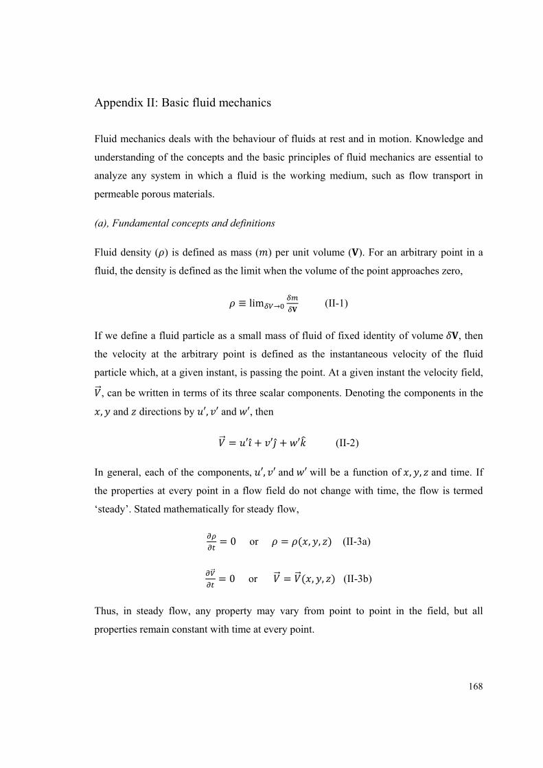
168

Appendix II: Basic fluid mechanics

Fluid mechanics deals with the behaviour of fluids at rest and in motion. Knowledge and

understanding of the concepts and the basic principles of fluid mechanics are essential to

analyze any system in which a fluid is the working medium, such as flow transport in

permeable porous materials.

(a), Fundamental concepts and definitions

Fluid density ( ) is defined as mass ( ) per unit volume ( ). For an arbitrary point in a

fluid, the density is defined as the limit when the volume of the point approaches zero,

≡ lim → (II-1)

If we define a fluid particle as a small mass of fluid of fixed identity of volume , then

the velocity at the arbitrary point is defined as the instantaneous velocity of the fluid

particle which, at a given instant, is passing the point. At a given instant the velocity field,

, can be written in terms of its three scalar components. Denoting the components in the , and directions by ′, ′ and ′, then

= ′ + ′ + ′ (II-2)

In general, each of the components, ′, ′ and ′ will be a function of , , and time. If

the properties at every point in a flow field do not change with time, the flow is termed

‘steady’. Stated mathematically for steady flow,

= 0 or = ( , , ) (II-3a)

= 0 or = ( , , ) (II-3b)

Thus, in steady flow, any property may vary from point to point in the field, but all

properties remain constant with time at every point.

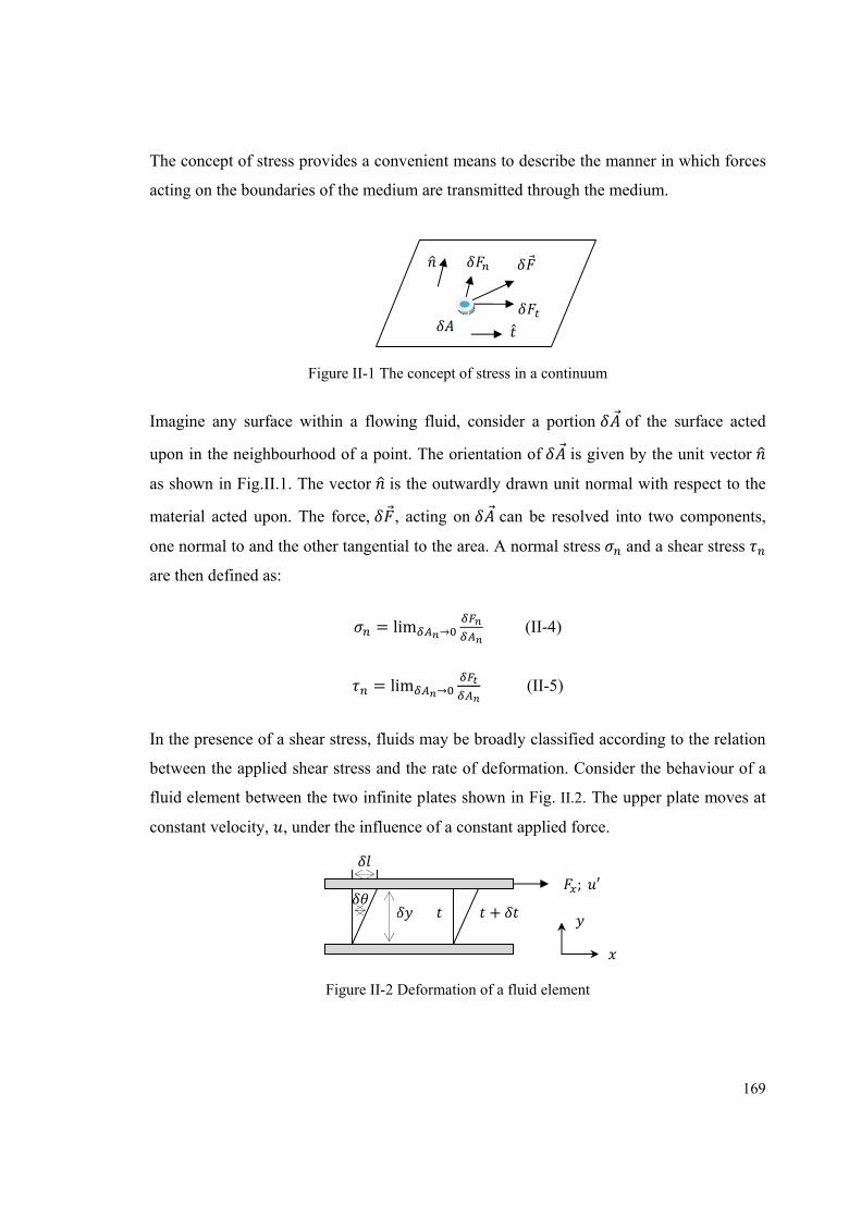
169

The concept of stress provides a convenient means to describe the manner in which forces

acting on the boundaries of the medium are transmitted through the medium.

Figure II-1 The concept of stress in a continuum

Imagine any surface within a flowing fluid, consider a portion of the surface acted

upon in the neighbourhood of a point. The orientation of is given by the unit vector

as shown in Fig.II.1. The vector is the outwardly drawn unit normal with respect to the

material acted upon. The force, , acting on can be resolved into two components,

one normal to and the other tangential to the area. A normal stress and a shear stress

are then defined as:

= lim → (II-4)

= lim → (II-5)

In the presence of a shear stress, fluids may be broadly classified according to the relation

between the applied shear stress and the rate of deformation. Consider the behaviour of a

fluid element between the two infinite plates shown in Fig. II.2. The upper plate moves at

constant velocity, , under the influence of a constant applied force.

Figure II-2 Deformation of a fluid element

+ ; ′

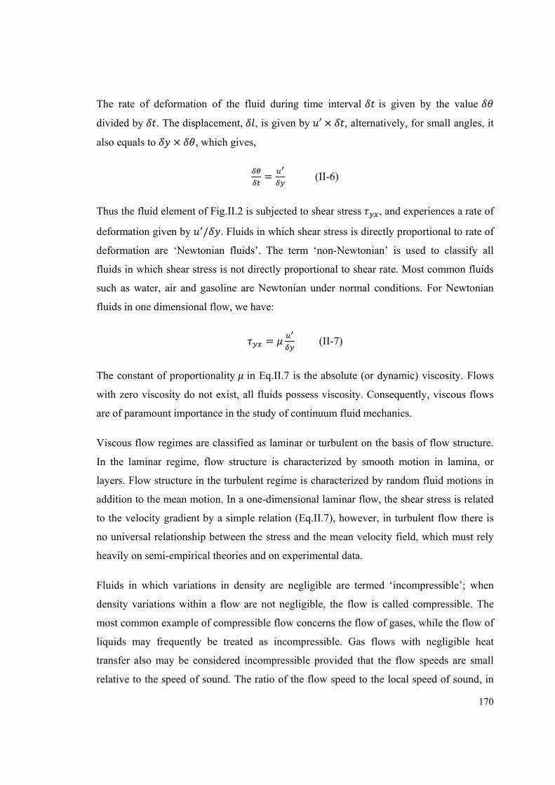
170

The rate of deformation of the fluid during time interval is given by the value

divided by . The displacement, , is given by ′ × , alternatively, for small angles, it

also equals to × , which gives,

= (II-6)

Thus the fluid element of Fig.II.2 is subjected to shear stress , and experiences a rate of

deformation given by / . Fluids in which shear stress is directly proportional to rate of

deformation are ‘Newtonian fluids’. The term ‘non-Newtonian’ is used to classify all

fluids in which shear stress is not directly proportional to shear rate. Most common fluids

such as water, air and gasoline are Newtonian under normal conditions. For Newtonian

fluids in one dimensional flow, we have:

= (II-7)

The constant of proportionality in Eq.II.7 is the absolute (or dynamic) viscosity. Flows

with zero viscosity do not exist, all fluids possess viscosity. Consequently, viscous flows

are of paramount importance in the study of continuum fluid mechanics.

Viscous flow regimes are classified as laminar or turbulent on the basis of flow structure.

In the laminar regime, flow structure is characterized by smooth motion in lamina, or

layers. Flow structure in the turbulent regime is characterized by random fluid motions in

addition to the mean motion. In a one-dimensional laminar flow, the shear stress is related

to the velocity gradient by a simple relation (Eq.II.7), however, in turbulent flow there is

no universal relationship between the stress and the mean velocity field, which must rely

heavily on semi-empirical theories and on experimental data.

Fluids in which variations in density are negligible are termed ‘incompressible’; when

density variations within a flow are not negligible, the flow is called compressible. The

most common example of compressible flow concerns the flow of gases, while the flow of

liquids may frequently be treated as incompressible. Gas flows with negligible heat

transfer also may be considered incompressible provided that the flow speeds are small

relative to the speed of sound. The ratio of the flow speed to the local speed of sound, in

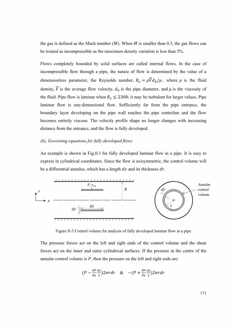
171

the gas is defined as the Mach number ( ). When is smaller than 0.3, the gas flows can

be treated as incompressible as the maximum density variation is less than 5%.

Flows completely bounded by solid surfaces are called internal flows. In the case of

incompressible flow through a pipe, the nature of flow is determined by the value of a

dimensionless parameter, the Reynolds number, = / , where is the fluid

density, is the average flow velocity, is the pipe diameter, and is the viscosity of

the fluid. Pipe flow is laminar when ≤ 2300; it may be turbulent for larger values. Pipe

laminar flow is one-dimensional flow. Sufficiently far from the pipe entrance, the

boundary layer developing on the pipe wall reaches the pipe centreline and the flow

becomes entirely viscous. The velocity profile shape no longer changes with increasing

distance from the entrance, and the flow is fully developed.

(b), Governing equations for fully developed flows

An example is shown in Fig.II.3 for fully developed laminar flow in a pipe. It is easy to

express in cylindrical coordinates. Since the flow is axisymmetric, the control volume will

be a differential annulus, which has a length and its thickness .

Figure II-3 Control volume for analysis of fully developed laminar flow in a pipe

The pressure forces act on the left and right ends of the control volume and the shear

forces act on the inner and outer cylindrical surfaces. If the pressure at the centre of the

annular control volume is , then the pressure on the left and right ends are:

( − )2 & −( + )2

Annular control volume

,

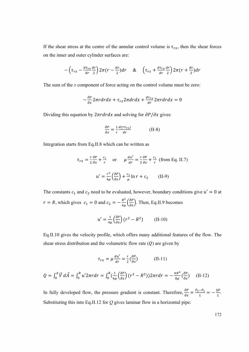
172

If the shear stress at the centre of the annular control volume is , then the shear forces

on the inner and outer cylinder surfaces are:

− − 2 ( − ) & + 2 ( + )

The sum of the x component of force acting on the control volume must be zero:

− 2 + 2 + 2 = 0

Dividing this equation by 2 and solving for / gives:

= ( ) (II-8)

Integration starts from Eq.II.8 which can be written as

= + or = + (from Eq. II.7)

′ = + ln + (II-9)

The constants and need to be evaluated, however, boundary conditions give ′ = 0 at = , which gives = 0 and = − . Then, Eq.II.9 becomes

′ = ( − ) (II-10)

Eq.II.10 gives the velocity profile, which offers many additional features of the flow. The

shear stress distribution and the volumetric flow rate ( ) are given by

= = ( ) (II-11)

= = ′2 = ( ( − ))2 = − ( ) (II-12)

In fully developed flow, the pressure gradient is constant. Therefore, = = −∆.

Substituting this into Eq.II.12 for Q gives laminar flow in a horizontal pipe:

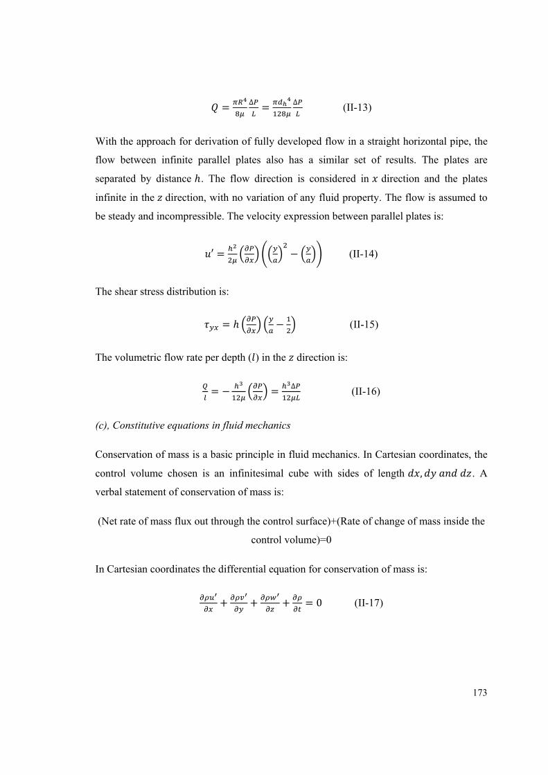
173

= ∆ = ∆ (II-13)

With the approach for derivation of fully developed flow in a straight horizontal pipe, the

flow between infinite parallel plates also has a similar set of results. The plates are

separated by distance ℎ. The flow direction is considered in direction and the plates

infinite in the direction, with no variation of any fluid property. The flow is assumed to

be steady and incompressible. The velocity expression between parallel plates is:

′ = − (II-14)

The shear stress distribution is:

= ℎ − (II-15)

The volumetric flow rate per depth ( ) in the direction is:

= − = ∆ (II-16)

(c), Constitutive equations in fluid mechanics

Conservation of mass is a basic principle in fluid mechanics. In Cartesian coordinates, the

control volume chosen is an infinitesimal cube with sides of length , . A

verbal statement of conservation of mass is:

(Net rate of mass flux out through the control surface)+(Rate of change of mass inside the

control volume)=0

In Cartesian coordinates the differential equation for conservation of mass is:

+ + + = 0 (II-17)

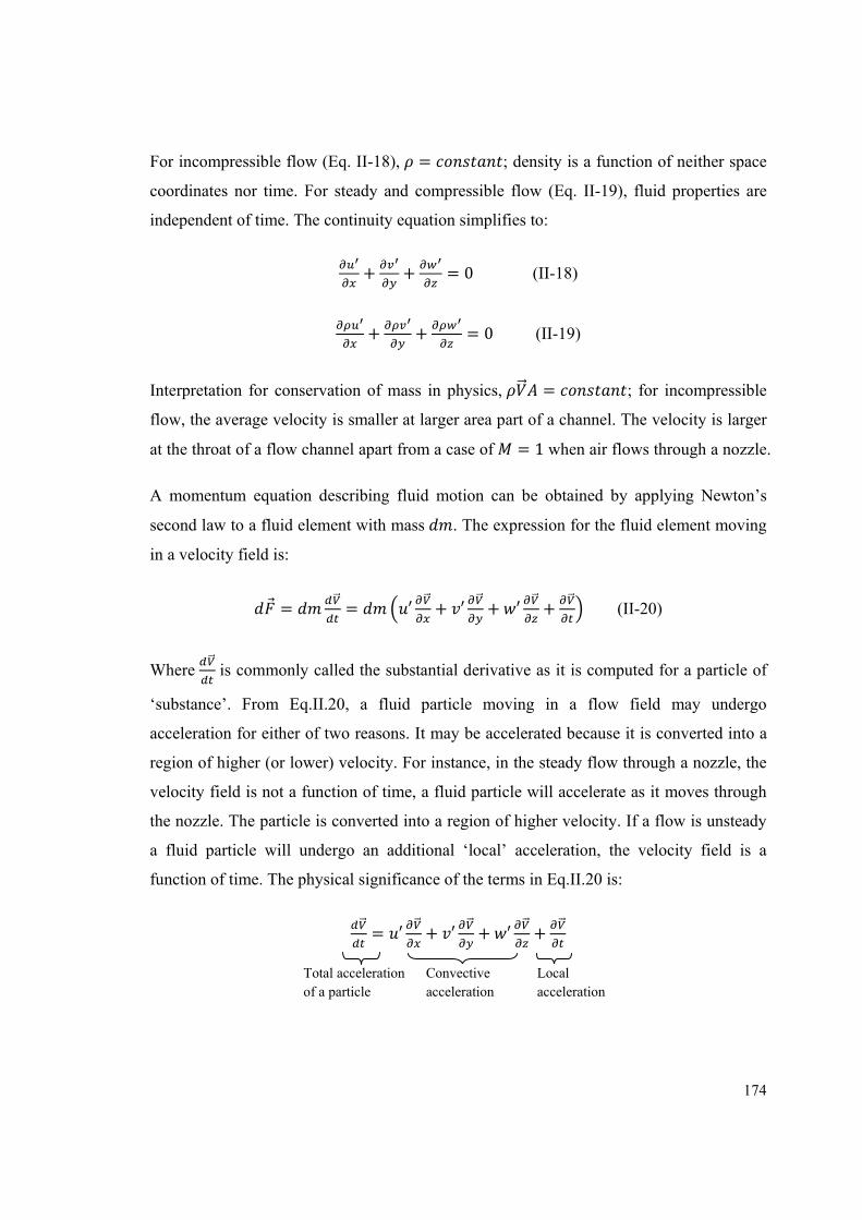
174

For incompressible flow (Eq. II-18), = ; density is a function of neither space

coordinates nor time. For steady and compressible flow (Eq. II-19), fluid properties are

independent of time. The continuity equation simplifies to:

+ + = 0 (II-18)

+ + = 0 (II-19)

Interpretation for conservation of mass in physics, = ; for incompressible

flow, the average velocity is smaller at larger area part of a channel. The velocity is larger

at the throat of a flow channel apart from a case of = 1 when air flows through a nozzle.

A momentum equation describing fluid motion can be obtained by applying Newton’s

second law to a fluid element with mass . The expression for the fluid element moving

in a velocity field is:

= = ′ + ′ + ′ + (II-20)

Where is commonly called the substantial derivative as it is computed for a particle of

‘substance’. From Eq.II.20, a fluid particle moving in a flow field may undergo

acceleration for either of two reasons. It may be accelerated because it is converted into a

region of higher (or lower) velocity. For instance, in the steady flow through a nozzle, the

velocity field is not a function of time, a fluid particle will accelerate as it moves through

the nozzle. The particle is converted into a region of higher velocity. If a flow is unsteady

a fluid particle will undergo an additional ‘local’ acceleration, the velocity field is a

function of time. The physical significance of the terms in Eq.II.20 is:

= ′ + ′ + ′ +

Total acceleration of a particle

Convective acceleration

Local acceleration

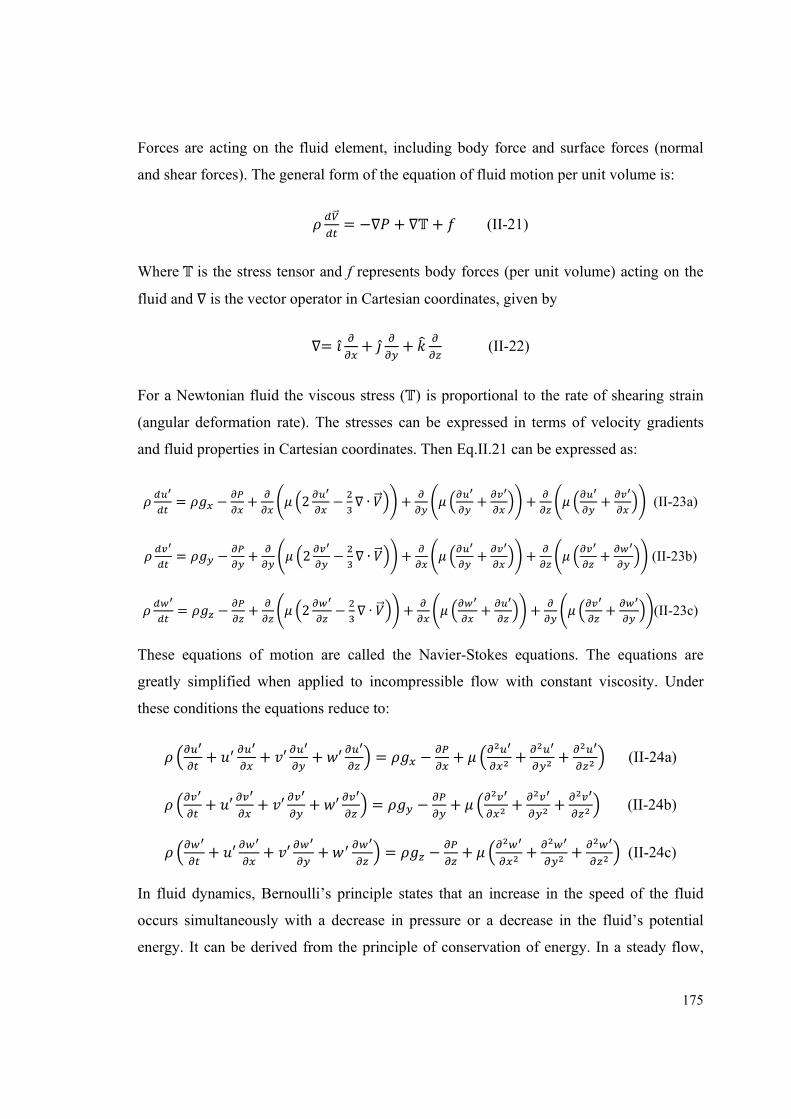
175

Forces are acting on the fluid element, including body force and surface forces (normal

and shear forces). The general form of the equation of fluid motion per unit volume is:

= −∇ + ∇ + (II-21)

Where is the stress tensor and f represents body forces (per unit volume) acting on the

fluid and ∇ is the vector operator in Cartesian coordinates, given by

∇= + + (II-22)

For a Newtonian fluid the viscous stress ( ) is proportional to the rate of shearing strain

(angular deformation rate). The stresses can be expressed in terms of velocity gradients

and fluid properties in Cartesian coordinates. Then Eq.II.21 can be expressed as:

= − + 2 − ∇ ∙ + + + + (II-23a)

= − + 2 − ∇ ∙ + + + + (II-23b)

= − + 2 − ∇ ∙ + + + + (II-23c)

These equations of motion are called the Navier-Stokes equations. The equations are

greatly simplified when applied to incompressible flow with constant viscosity. Under

these conditions the equations reduce to:

+ + ′ + ′ = − + + + (II-24a)

+ ′ + ′ + ′ = − + + + (II-24b)

+ ′ + ′ + = − + + + (II-24c)

In fluid dynamics, Bernoulli’s principle states that an increase in the speed of the fluid

occurs simultaneously with a decrease in pressure or a decrease in the fluid’s potential

energy. It can be derived from the principle of conservation of energy. In a steady flow,

176

this states that the sum of all forms of mechanical energy in a fluid along a streamline is

the same at all points on that streamline. This requires the sum of kinetic energy and

potential energy to remain constant:

+ + = (II-25)

The restrictions for Eq.II.25 are (1) steady flow; (2) incompressible flow; (3) frictionless

flow; (4) flow along a streamline. However, the Bernoulli equation is powerful because it

relates pressure changes to velocity and elevation changes a streamline due to the gravity

acceleration.

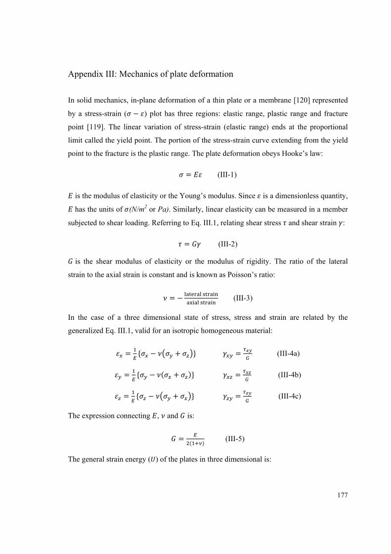
177

Appendix III: Mechanics of plate deformation

In solid mechanics, in-plane deformation of a thin plate or a membrane [120] represented

by a stress-strain ( − ) plot has three regions: elastic range, plastic range and fracture

point [119]. The linear variation of stress-strain (elastic range) ends at the proportional

limit called the yield point. The portion of the stress-strain curve extending from the yield

point to the fracture is the plastic range. The plate deformation obeys Hooke’s law: = (III-1)

is the modulus of elasticity or the Young’s modulus. Since is a dimensionless quantity,

has the units of (N/m2 or Pa). Similarly, linear elasticity can be measured in a member

subjected to shear loading. Referring to Eq. III.1, relating shear stress and shear strain : = (III-2)

is the shear modulus of elasticity or the modulus of rigidity. The ratio of the lateral

strain to the axial strain is constant and is known as Poisson’s ratio:

= − (III-3)

In the case of a three dimensional state of stress, stress and strain are related by the

generalized Eq. III.1, valid for an isotropic homogeneous material:

= { − + } = (III-4a) = { − ( + )} = (III-4b) = { − + } = (III-4c)

The expression connecting , and is:

= ( ) (III-5)

The general strain energy ( ) of the plates in three dimensional is:

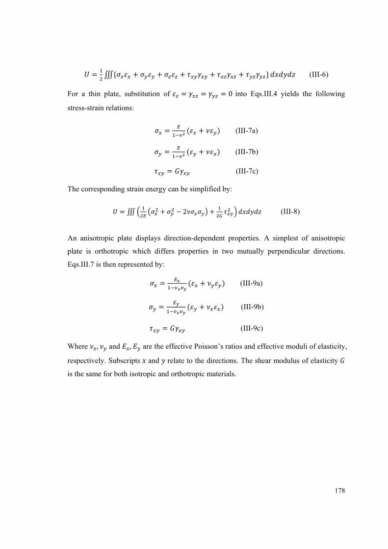
178

= ∭{ + + + + + } (III-6)

For a thin plate, substitution of = = = 0 into Eqs.III.4 yields the following

stress-strain relations:

= ( + ) (III-7a) = ( + ) (III-7b) = (III-7c)

The corresponding strain energy can be simplified by:

=∭ + − 2 + (III-8)

An anisotropic plate displays direction-dependent properties. A simplest of anisotropic

plate is orthotropic which differs properties in two mutually perpendicular directions.

Eqs.III.7 is then represented by: = ( + ) (III-9a)

= ( + ) (III-9b)

= (III-9c)

Where , and , are the effective Poisson’s ratios and effective moduli of elasticity,

respectively. Subscripts and relate to the directions. The shear modulus of elasticity

is the same for both isotropic and orthotropic materials.

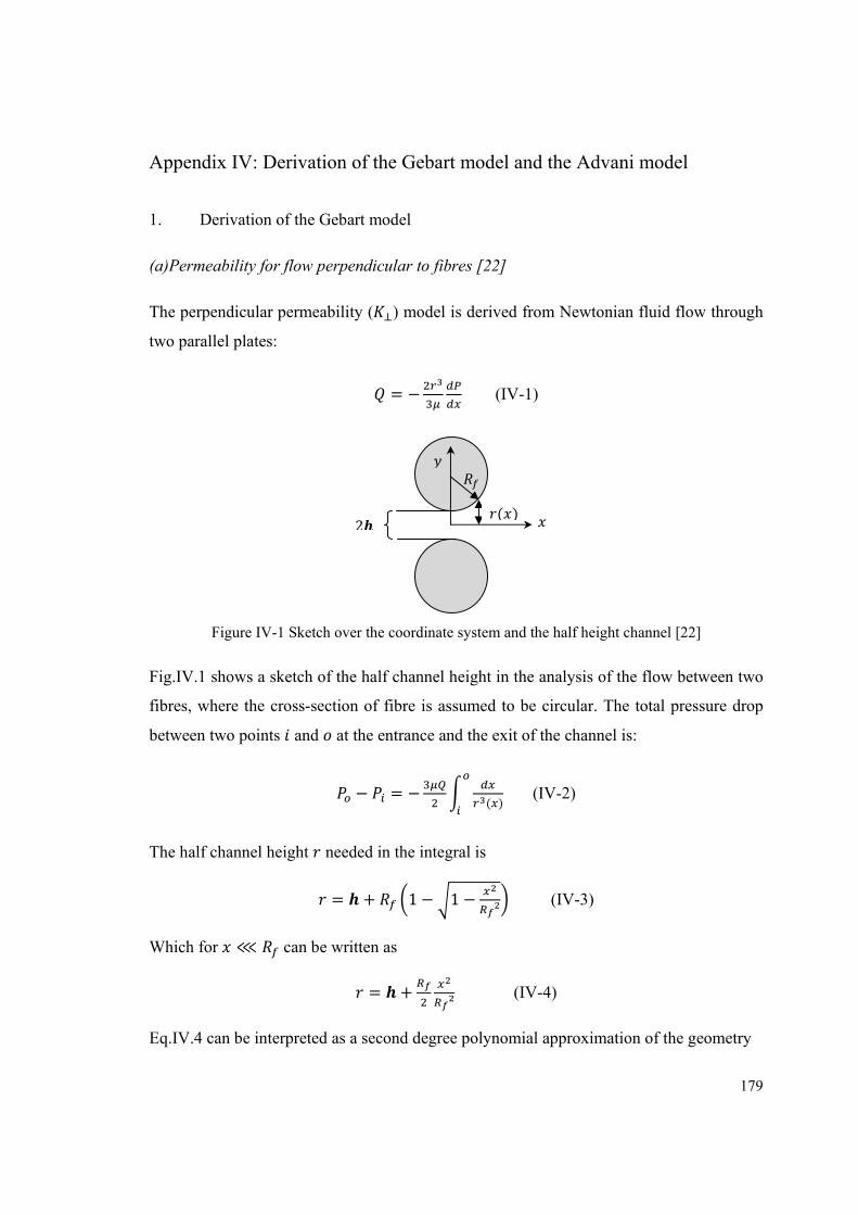
179

Appendix IV: Derivation of the Gebart model and the Advani model

1. Derivation of the Gebart model

(a)Permeability for flow perpendicular to fibres [22]

The perpendicular permeability ( ) model is derived from Newtonian fluid flow through

two parallel plates:

= − (IV-1)

Figure IV-1 Sketch over the coordinate system and the half height channel [22]

Fig.IV.1 shows a sketch of the half channel height in the analysis of the flow between two

fibres, where the cross-section of fibre is assumed to be circular. The total pressure drop

between two points and at the entrance and the exit of the channel is:

− = − ( ) (IV-2)

The half channel height needed in the integral is

= + 1 − 1 − (IV-3)

Which for ⋘ can be written as = + (IV-4)

Eq.IV.4 can be interpreted as a second degree polynomial approximation of the geometry

2 ( )

180

for circular fibres. Substitution of Eq.IV.4 in Eq.IV.2 and a simple change for the variables

makes it possible to rewrite the integral so that Eq.IV.2 becomes:

− = − ( ) (IV-5)

The author stated that most of the contributions to the integral come from the narrow gap

between the fibres if / ⋘ 1. Moreover, if the integral limits were taken as -2 to 2, the

integration will be 1.178, slightly larger than the real value 1.170. Therefore, 3 /8 ≈1.178 was used to substitute the integration in Eq.IV.5:

∆ = − √ ( ) / (IV-6)

Based on the definition of Darcy’s law, the permeability for the quadratic fibre

arrangement can be identified from Eq.IV.6 as:

= √ ( ) / (IV-7a)

= √ − 1 / (IV-7b)

Where is the maximum fibre volume fraction /4 when the fibres touch each other.

For a hexagonal array, the distance of inlet width of the unit cell is √3/2 times higher than

it in the quadratic arrangement, which gives the permeability ( ):

= √ ( ) / (IV-8a)

= √ − 1 / (IV-8b)

Where the value for the hexagonal arrangement is 2√3⁄ .

(b)Permeability for flow along fibres[22]

181

Analysis of permeability along unidirectional fibres ( ∥) starts from the frictional loss in a

duct within which a Newtonian fluid flows with arbitrary cross-section. The duct formed

in the space between the fibres, is usually expressed in terms of a frictional factor which

can be derived analytically for many cross-sections (circular, triangular, quadratic, etc.) in

laminar flows and can generally be expressed as:

= = ∆ (IV-9)

Where is the hydraulic diameter to be defined as four times the duct cross-sectional

area ’ divided by the wetted perimeter. ’ is the part of the total cross-section through

which fluid can flow, and differs from the area A used in the definition of Darcy’s law,

which is the total cross-section area of the sample including solid fibres. The ratio of the

two areas can be expressed in terms of fibre volume fraction:

= 1 − (IV-10)

Then the hydraulic diameter can be expressed as:

= ( ) (IV-11)

Where c is a dimensionless shape factor and is the Reynolds number. Substitution of

Eq. IV.11 into Eq. IV.10 and identification of the permeability yields:

∥ = ( ) (IV-12)

Gebart computed (numerically) the value of the shape factor c for any fibre volume

fraction both in the quadratic and the hexagonal cases and obtained = 53 for the

hexagonal arrangement and = 57 for the quadratic arrangement, respectively. Eq. IV.12

has the similar style with the Kozeny-Carman equation (Eq.2.2), where the shape factor c

is related to the Kozeny constant as = 32 .

2. Derivation of the Advani model

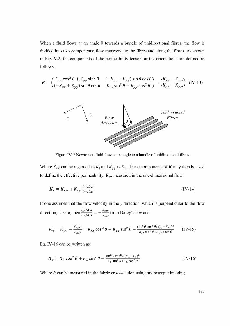
182

When a fluid flows at an angle θ towards a bundle of unidirectional fibres, the flow is

divided into two components: flow transverse to the fibres and along the fibres. As shown

in Fig.IV.2, the components of the permeability tensor for the orientations are defined as

follows:

= cos + sin (− + ) sin cos(− + ) sin cos sin + cos = (IV-13)

Figure IV-2 Newtonian fluid flow at an angle to a bundle of unidirectional fibres

Where can be regarded as ∥ and is . These components of may then be used

to define the effective permeability, , measured in the one-dimensional flow:

= + // (IV-14)

If one assumes that the flow velocity in the y direction, which is perpendicular to the flow

direction, is zero, then // = − from Darcy’s law and:

= − = cos + sin − ( ) (IV-15)

Eq. IV-16 can be written as:

= ∥ cos + sin − ( ∥)∥ (IV-16)

Where can be measured in the fabric cross-section using microscopic imaging.

Unidirectional Fibres

θ

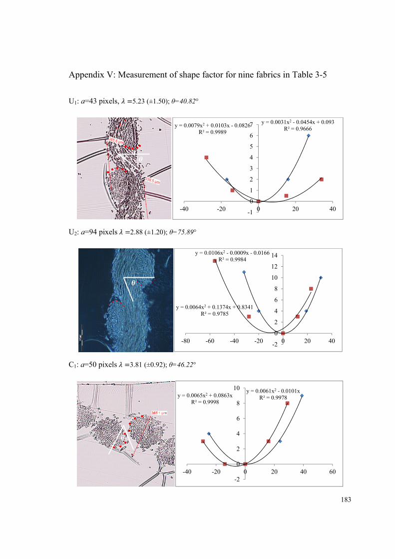
183

Appendix V: Measurement of shape factor for nine fabrics in Table 3-5

U1: a=43 pixels, =5.23 (±1.50); θ=40.82°

U2: a=94 pixels =2.88 (±1.20); θ=75.89°

C1: a=50 pixels =3.81 (±0.92); θ=46.22°

y = 0.0079x2 + 0.0103x - 0.0826R² = 0.9989

y = 0.0031x2 - 0.0454x + 0.093R² = 0.9666

-1

0

1

2

3

4

5

6

7

-40 -20 0 20 40

y = 0.0106x2 - 0.0009x - 0.0166R² = 0.9984

y = 0.0064x2 + 0.1374x + 0.8341R² = 0.9785

-2

0

2

4

6

8

10

12

14

-80 -60 -40 -20 0 20 40

y = 0.0061x2 - 0.0101xR² = 0.9978y = 0.0065x2 + 0.0863x

R² = 0.9998

-2

0

2

4

6

8

10

-40 -20 0 20 40 60

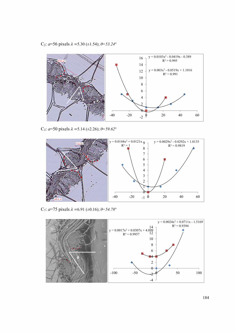
184

C2: a=56 pixels =5.30 (±1.54); θ=53.24°

C3: a=50 pixels =5.14 (±2.26); θ=59.62°

C7: a=75 pixels =6.91 (±0.16); θ=54.78°

y = 0.003x2 - 0.0519x + 1.1016R² = 0.991

y = 0.0103x2 - 0.0419x - 0.389R² = 0.995

-2

0

2

4

6

8

10

12

14

16

-40 -20 0 20 40 60

y = 0.0029x2 - 0.0292x + 1.0135R² = 0.9819

y = 0.0144x2 + 0.0121xR² = 1

-1

0

1

2

3

4

5

6

7

8

9

-40 -20 0 20 40 60

y = 0.0024x2 + 0.0711x - 1.5169R² = 0.9394

y = 0.0017x2 + 0.0307x + 4.099R² = 0.9957

-4

-2

0

2

4

6

8

10

12

14

-100 -50 0 50 100

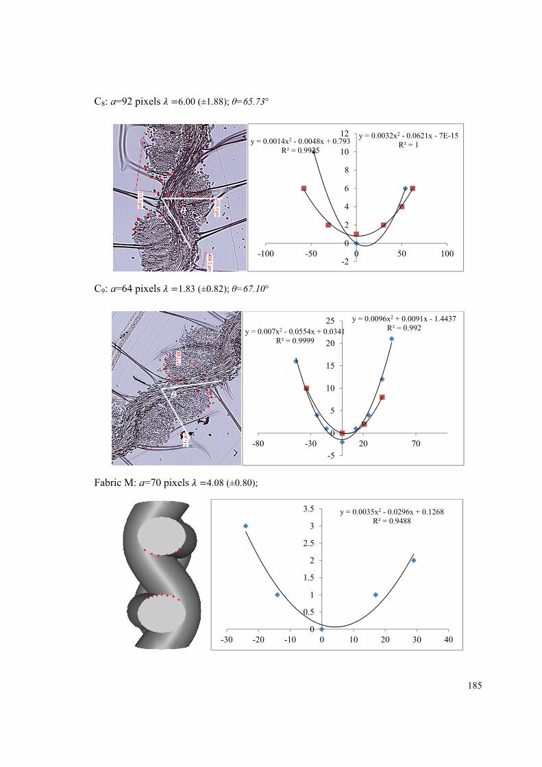
185

C8: a=92 pixels =6.00 (±1.88); θ=65.73°

C9: a=64 pixels =1.83 (±0.82); θ=67.10°

Fabric M: a=70 pixels =4.08 (±0.80);

y = 0.0032x2 - 0.0621x - 7E-15R² = 1y = 0.0014x2 - 0.0048x + 0.793

R² = 0.9925

-2

0

2

4

6

8

10

12

-100 -50 0 50 100

y = 0.0096x2 + 0.0091x - 1.4437R² = 0.992y = 0.007x2 - 0.0554x + 0.0341

R² = 0.9999

-5

0

5

10

15

20

25

-80 -30 20 70

y = 0.0035x2 - 0.0296x + 0.1268R² = 0.9488

0

0.5

1

1.5

2

2.5

3

3.5

-30 -20 -10 0 10 20 30 40

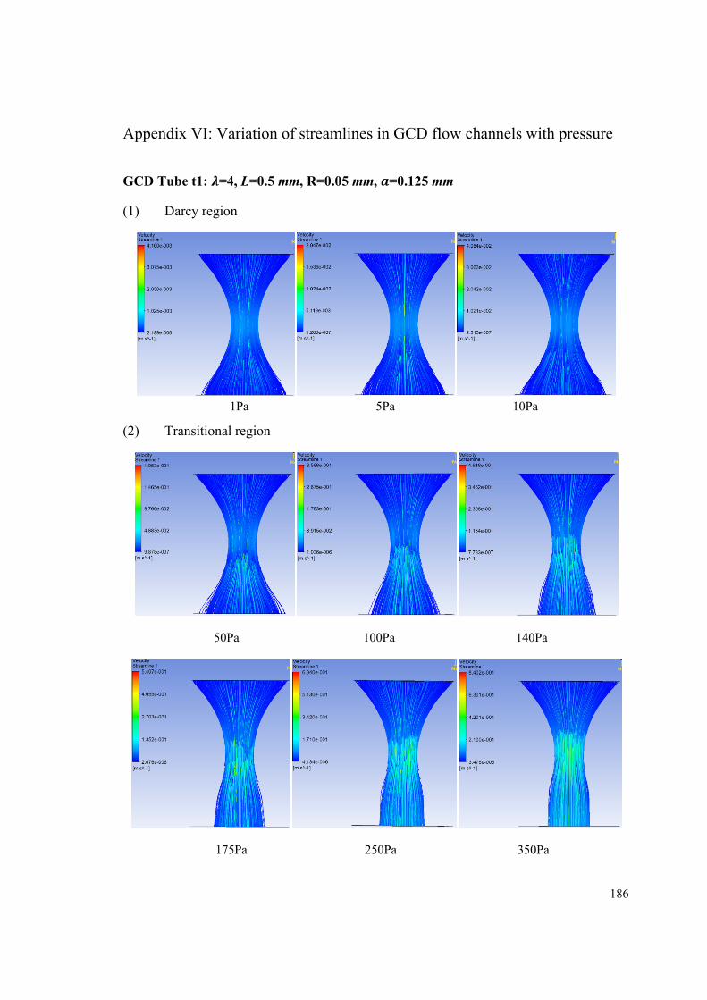
186

Appendix VI: Variation of streamlines in GCD flow channels with pressure

GCD Tube t1: =4, L=0.5 mm, R=0.05 mm, =0.125 mm

(1) Darcy region

1Pa 5Pa 10Pa

(2) Transitional region

50Pa 100Pa 140Pa

175Pa 250Pa 350Pa

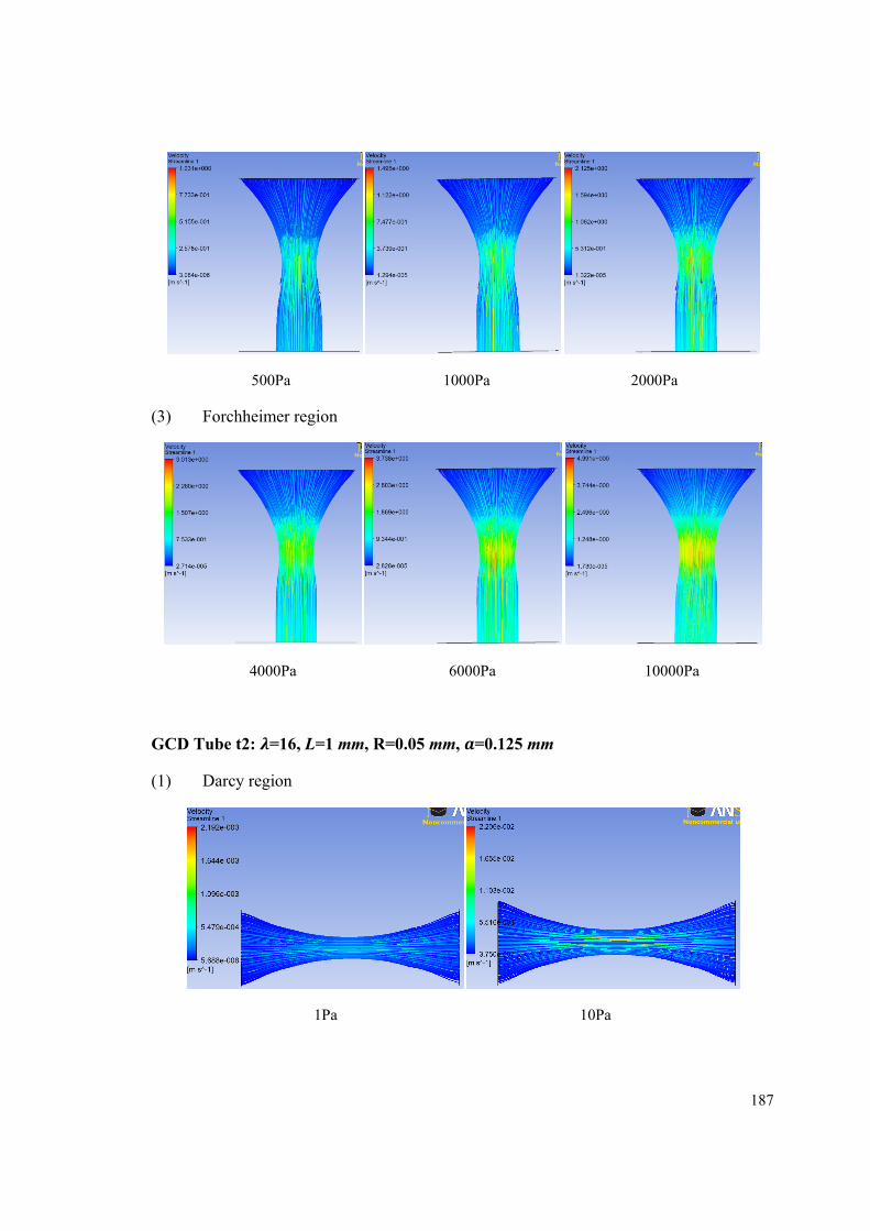
187

500Pa 1000Pa 2000Pa

(3) Forchheimer region

4000Pa 6000Pa 10000Pa

GCD Tube t2: =16, L=1 mm, R=0.05 mm, =0.125 mm

(1) Darcy region

1Pa 10Pa

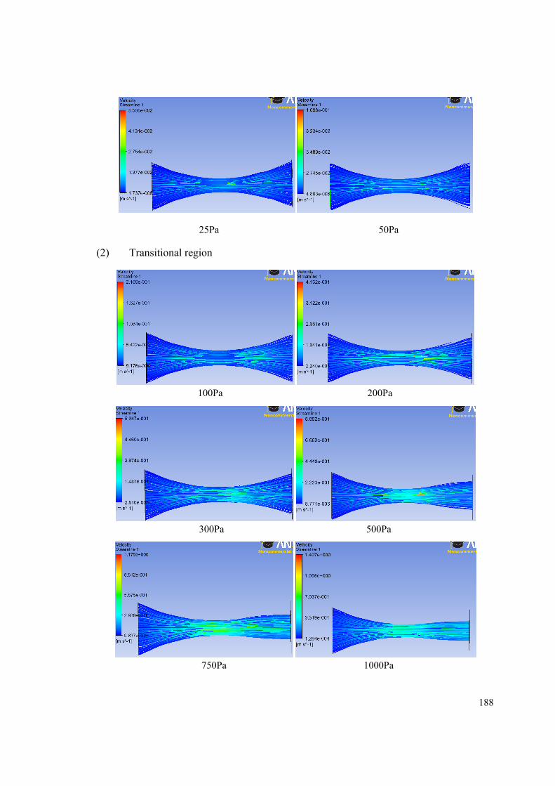
188

25Pa 50Pa

(2) Transitional region

100Pa 200Pa

300Pa 500Pa

750Pa 1000Pa

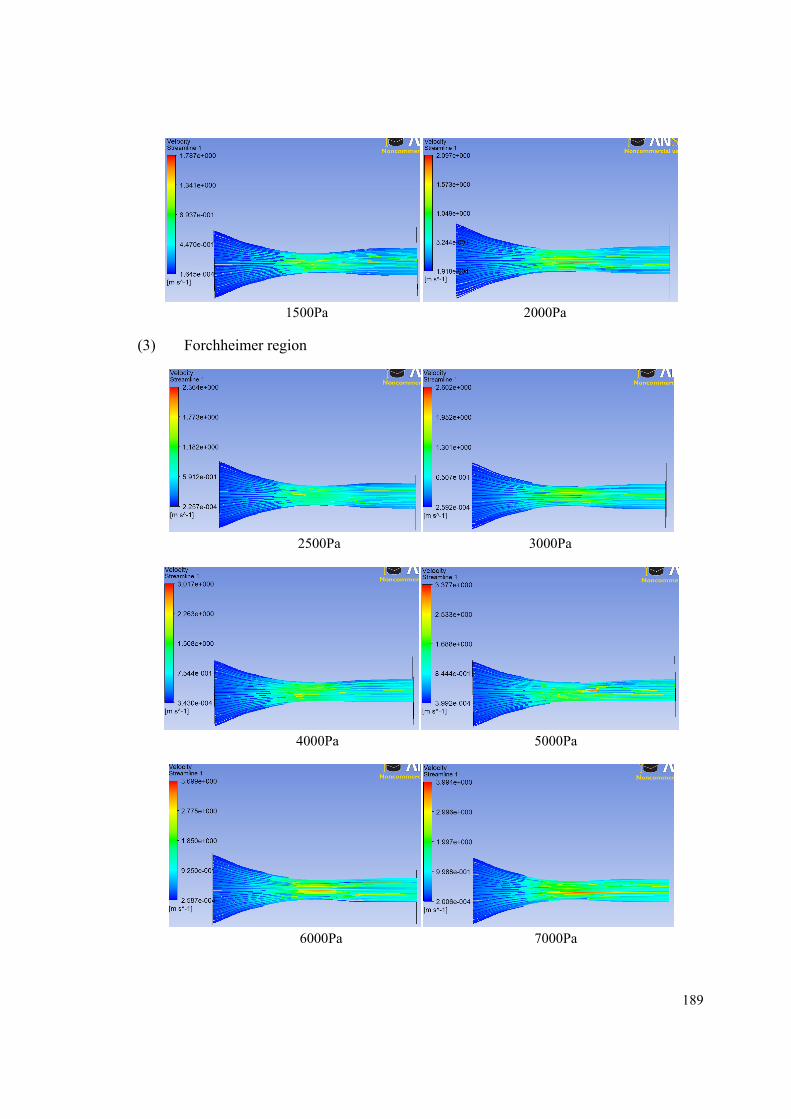
189

1500Pa 2000Pa

(3) Forchheimer region

2500Pa 3000Pa

4000Pa 5000Pa

6000Pa 7000Pa

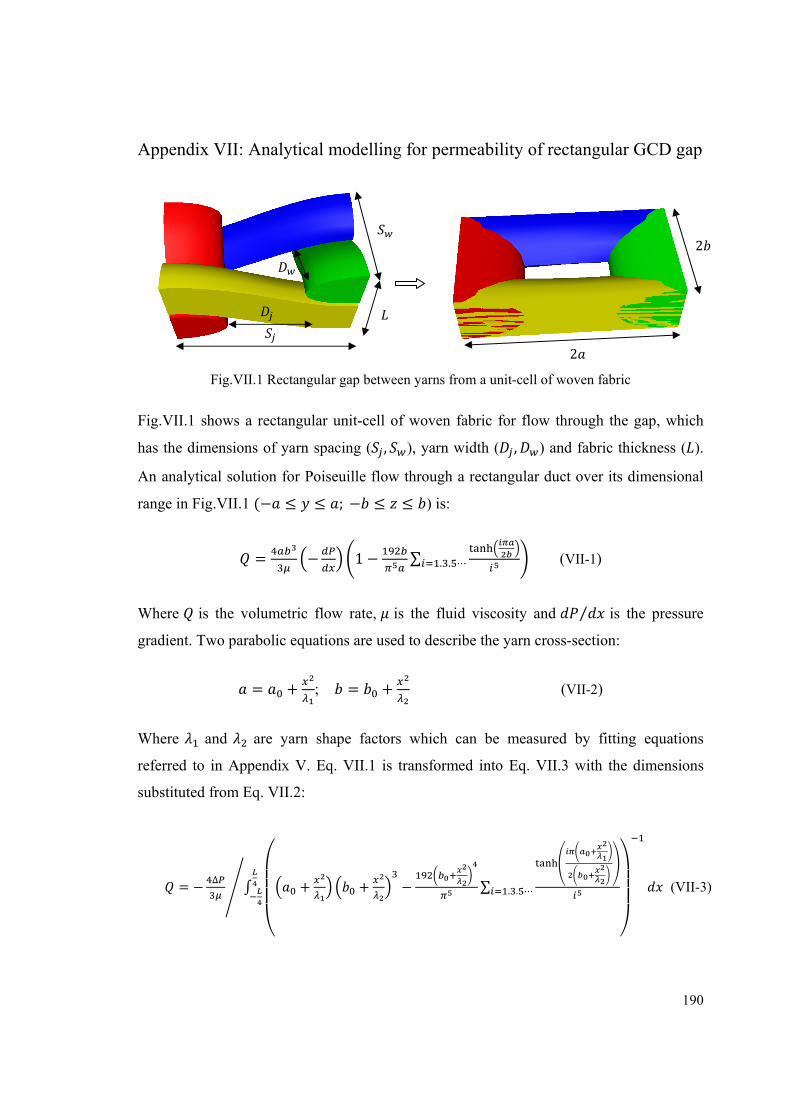
190

Appendix VII: Analytical modelling for permeability of rectangular GCD gap

Fig.VII.1 Rectangular gap between yarns from a unit-cell of woven fabric

Fig.VII.1 shows a rectangular unit-cell of woven fabric for flow through the gap, which

has the dimensions of yarn spacing ( , ), yarn width ( , ) and fabric thickness ( ).

An analytical solution for Poiseuille flow through a rectangular duct over its dimensional

range in Fig.VII.1 (− ≤ ≤ ;− ≤ ≤ ) is:

= − 1 − ∑ . . ⋯ (VII-1)

Where is the volumetric flow rate, is the fluid viscosity and ⁄ is the pressure

gradient. Two parabolic equations are used to describe the yarn cross-section:

= + ; = + (VII-2)

Where and are yarn shape factors which can be measured by fitting equations

referred to in Appendix V. Eq. VII.1 is transformed into Eq. VII.3 with the dimensions

substituted from Eq. VII.2:

= − ∆ + + − ∑ . . ⋯ (VII-3)

2

2

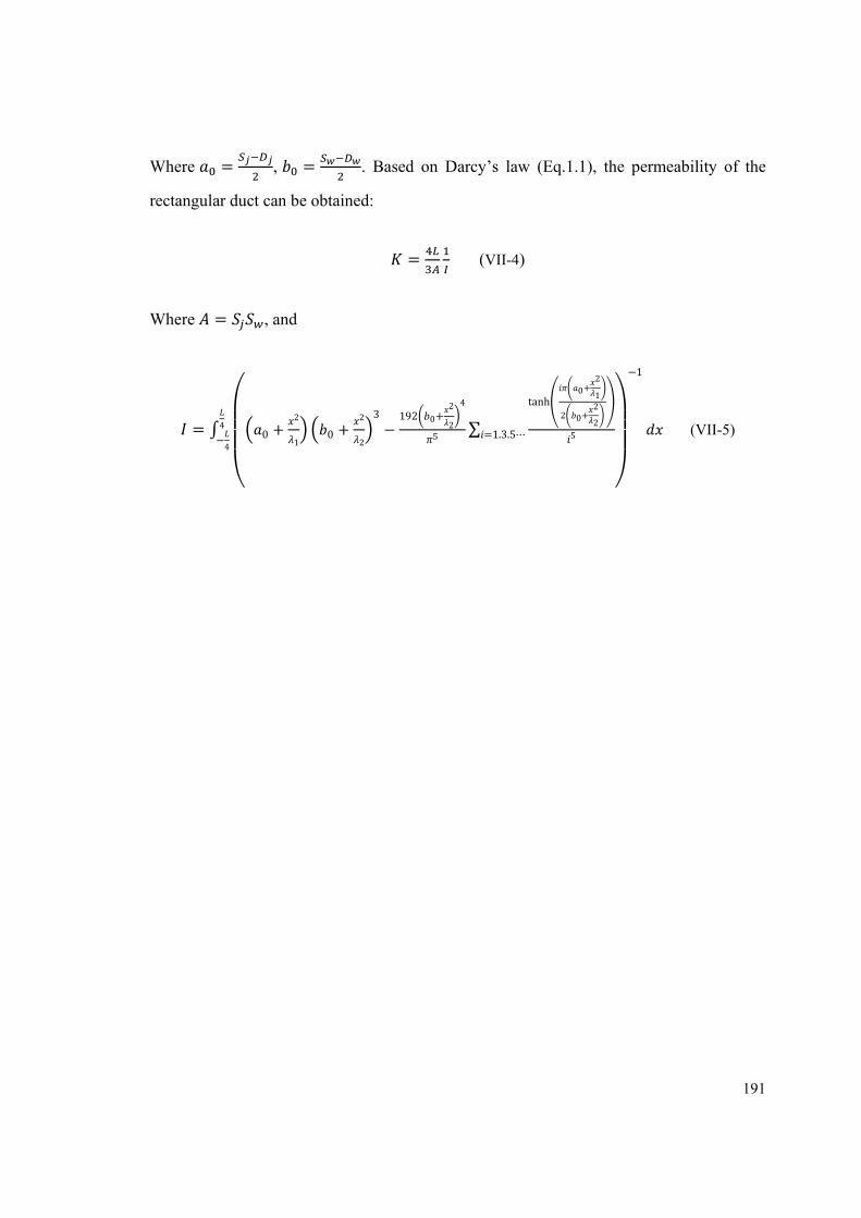
191

Where = , = . Based on Darcy’s law (Eq.1.1), the permeability of the

rectangular duct can be obtained:

= (VII-4)

Where = , and

= 0 + 21 0 + 223 − 192 0+ 22 4

5 ∑ tanh 0+ 212 0+ 225=1.3.5⋯−1

4−4 (VII-5)