Astronomy & Astrophysics manuscript no. aa ©ESO 2021October 8, 2021

Modeling the Mg i from the NUV to MIR: I. The Solar CaseJ.I. Peralta1, 2, Vieytes M.C.1, 2, A.M.P. Mendez1, and D.M. Mitnik1, 3

1 Instituto de Astronomía y Física del Espacio, CONICET–Universidad de Buenos Aires, Argentinae-mail: jperalta@iafe.uba.ar; mariela@iafe.uba.ar

2 Departamento de Ciencia y Tecnología, UNTREF, Argentina3 Departamento de Física, Universidad de Buenos Aires, Argentina

Received 6 August 2021, Accepted 6 October 2021

ABSTRACT

Context. Semi-empirical models of the solar atmosphere are used to study the radiative environment of any planet in our solar system.There is a need for reliable atomic data for neutral atoms and ions in the atmosphere to obtain improved calculated spectra. Atomicparameters are crucial to computing the correct population of elements through the whole stellar atmosphere. Although there is a verygood agreement between the observed and calculated spectra for the Sun, there is still a mismatch in several spectral ranges due tothe lack of atomic data and its inaccuracies, particularly for neutrals like Mg i.Aims. To correctly represent many spectral lines of Mg i from the near-UV to the mid-IR is necessary to add and update the atomicdata involved in the atomic processes that drive their formation.Methods. The improvements to the Mg i atomic model are as follows: i) 127 strong lines, including their broadening data, wereadded. ii) To obtain these new lines, we increased from 26 to 85 the number of energy levels. iii) Photoionization cross-sectionparameters were added and updated. iv) Effective Collision Strengths (Υi j) parameters were updated for the first 25 levels using theexisting data from the convergent close-coupling (CCC) calculations. One of the most significant changes in our model is given by thenew Υi j parameters for transitions involving levels between 26 and 54, which were computed with a multi–configuration Breit–Paulidistorted–wave (DW) method. For transitions involving superlevels, we calculated the Υi j parameters with the usual semi-empiricalformulas of Seaton (1962) and van Regemorter (1962).Results. More than one hundred transitions were added to our calculations, increasing our capability of reproducing important featuresobserved in the solar spectra. We found a remarkable improvement in matching the solar spectra for wavelengths higher than 30 000Å when our new DW Υi j data was used in the model.Conclusions.

Key words. atomic:data – sun:atmospheres – Sun:infrared – line:formation – line:profile

1. Introduction

1D semi-empirical model calculation of the solar atmospherecontinues to be useful to predict and reproduce the Solar Spec-tral Irradiance (SSI), from the far-infrared (FIR) to the extremeultraviolet (EUV), received at the top of the Earth’s atmosphere(Fontenla & Landi 2018). Changes in the SSI can produce mod-ifications in the chemistry of our atmosphere.

The advantage of these models is that they are built to repro-duce a large number of observations in different wavelengths.The equations of statistical equilibrium and radiative transfer aretreated in detail and solved simultaneously for all the species inthe atmosphere. One of the most critical parameters is the datadescribing the atomic and molecular species present in the at-mosphere. Great efforts have been made to obtain experimentaland theoretical data. However, there is still a lack of completeand accurate atomic data, particularly for neutral and low ion-ized atoms. These atomic species, such as Mg i, are of particu-lar interest because they have relevant spectral features used inthe diagnosis of solar and stellar astrophysics. The influence ofusing a more complete and accurate atomic model for neutralatoms in SSI calculations can be found, for example, in Vieytes& Fontenla (2013), were the improvements made in the Ni iatomic model led to a better match with observations, mainlyin the near-ultraviolet (NUV) region.

Neutral magnesium is an important chemical element sinceits lines are strong in the spectra of late-type and even in metal-poor stars, making it a good tracer of α-element abundances. Atchromospheric temperatures, magnesium is susceptible to devi-ations from local thermodynamic equilibrium (LTE). These de-viations from LTE are predicted to be significant, particularlyfor metal-poor stars (Zhao et al. 1998; Zhao & Gehren 2000).Therefore to study the non-LTE (NLTE) effects it is necessary toaccount for accurate atomic data.

Past studies have used semi-empirical formulae when com-puting electron atomic collision data. The most widely usedsemi-classical formulas for radiative allowed transitions are theones given by Seaton (1962) and van Regemorter (1962) sincethey provide estimates for the collision rates based on the oscilla-tor strengths and transition energies. However, these approxima-tions can lead to a great number of uncertainties in the syntheticspectra of NLTE atmospheric models, such as spectral lines inemission instead of in absorption as observations reveal.

There are several studies on NLTE calculations of Mg i in theSun and other stars, for instance, the recent works by Alexeevaet al. (2018), the paper series by Osorio et al. (2015), Osorio& Barklem (2016) and Barklem et al. (2017), and the relevantworks by Bergemann et al. (2015) and Scott et al. (2015). Inall of these studies, the authors stress the need for accurate Mg iatomic data.

Article number, page 1 of 14

arX

iv:2

110.

0299

2v1

[as

tro-

ph.S

R]

6 O

ct 2

021

A&A proofs: manuscript no. aa

Osorio et al. (2015) described in detail previous studies ofNLTE Mg i line formation. They presented a complete Mg iatomic model of 108 energetic states (including fine-structuresplitting), up to level 20d. Among other important improve-ments, they included new electron impact values for low-lyingstates using the R-Matrix method. For transitions involvingstates greater than 5p 3P the data was complemented with theSeaton (1962) formula. The authors analyzed relevant spectrallines from ∼3800 Å to ∼8800 Å including the mid-IR (MIR)lines: 7.3, 12.2, 12.3, 18.8, 18.96 µm. The NLTE calculation wascomputed using the MULTI code (Carlsson 1992). Their syn-thetic spectra showed a good agreement with solar observationsand with observations of five F-G-K late-type stars with reliablefundamental parameters. Barklem et al. (2017) presented the lat-est calculations for inelastic e+Mg for the first 25 energy statesof neutral magnesium (up to 3s6p 1P), produced by the con-vergent close-coupling (CCC) and the B-spline R-matrix (BSR)methods. In this work, the authors suggest their CCC data forNLTE modeling.

Later, Alexeeva et al. (2018) made an extensive study ofNLTE Mg i line formation in the Sun and 17 stars, covering B-A-F-G-K spectral types. They used an atomic model of about 89energetic states, up to level n = 16. For electronic collisions, theyimplemented data from Osorio et al. (2015) and complementedwith data from Seaton (1962) formula for allowed transitions. Inthe case of forbidden transitions, the authors assumed a singlevalue for the effective collision strength, being Υi j = 1. To testtheir results they also selected spectral lines starting at ∼3800 Åuntil ∼8800 Å, and included the MIR lines: 7.3, 12.2, 12.3 µm.The NLTE calculation was made using the DETAIL code (Butler& Giddings 1985).

None of the previous works on Mg i line formation repro-duces spectral lines in the NUV region or lines between ∼8800Å and 7.3 µm in the NIR and MIR. Nevertheless, the NUV playsa fundamental role in ozone formation, and any calculation ofthe SSI must reproduce this region as well as possible.

Everything we know about our Sun and its relationship withthe Earth’s atmosphere can be extended and applied to study theatmosphere of exoplanets orbiting around late-type stars. Thesame methodology is used to calculate the Spectral Energy Dis-tribution (SED) that an exoplanet orbiting a late-type star re-ceives at the top of its atmosphere (Tilipman et al. 2021).

Nonetheless, our Sun can be observed with unique spatialand spectral resolution. For this reason, changes in the atomicmodels included in the atmospheric modeling must first be testedto reproduce the observed solar spectra.

The goal of the present work is two folded. We intend to up-date the Mg i atomic model. Consequently, we expect to extendthe analysis of spectral line formation of Mg i to include tran-sitions in a broader range than previous studies, from the NUV(1700 Å) to MIR (72 000 Å).

Regarding the electronic collisions, we included two signifi-cant improvements to the electron impact excitation data. Fromour original atomic model, we replaced the semi-empirical ef-fective collision strength (Υi j) values for the first 25 lower-lyingterms by close-coupling calculations (Barklem et al. 2017). Fur-thermore, we used the autostructure code (Badnell 2011) tocalculate collisional strengths under the distorted wave approx-imation. We incorporated these results by replacing the semi-empirical Υi j involving states between 3s6p and 3s7i.

This paper is structured as follows: The code used in ourNLTE and spectra calculations together with the initial atomicmodel is detailed in Section 2. Section 3 shows the different Mg i

0 500 1000 1500 2000Height (km)

104

4 × 103

6 × 103

2 × 104

Tem

pera

ture

(K)

Photosphere ChromosphereTransition

region

Model 1401

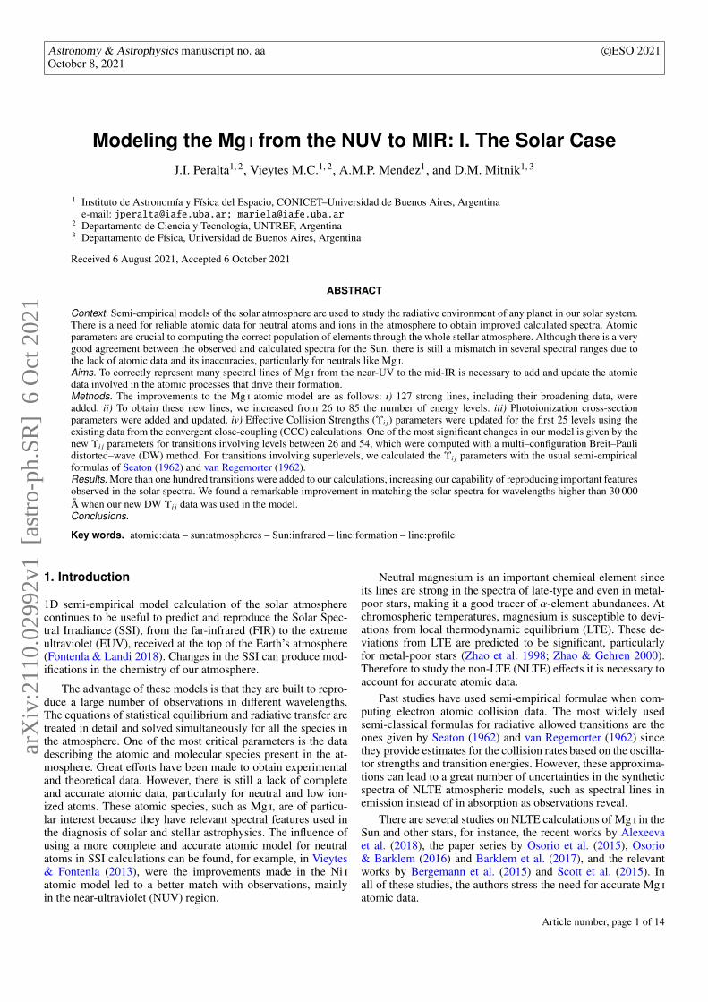
Fig. 1. Atmospheric model 1401 by Fontenla et al. (2015). Models inthis work have the same thermal structure than 1401.

Fig. 2. Distribution of changes between the original and the updated Acoefficients with wavelength included in model 1401a.

atomic models built. The observations used to compare with oursynthetic spectra are described in Section 4. Our results and dis-cussion are presented in Section 5, while our final remarks andconclusions are shown in Section 6.

2. NLTE and initial emergent spectra calculations

2.1. SRPM system and the solar model employed

We carried out the NLTE and spectra calculations by makinguse of the Solar Radiation Physical Modeling (SRPM) version 2system, a first version developed by Fontenla & Harder (2005),and later updated by Fontenla et al. (2015). This system is a li-brary of codes that allows us to calculate self-consistently theequations of statistical equilibrium and radiative transfer for aplane-parallel or spherical symmetric atmosphere, assuming hy-drostatic equilibrium.

One key point of the SRPM system is that it computes fullNLTE for all atomic species in the atmosphere, based on theNet Radiative Bracket Operator formulation implemented by

Article number, page 2 of 14

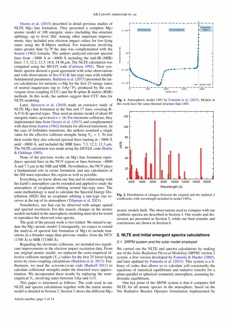
J.I. Peralta et al.: Modeling the Mg i from the NUV to MIR: I. The Solar Case

Model Mg i levs Mg ii levs Υi j methods (Mg i) Notes

1401 26 14 SEA&VRM Original model in Fontenla et al. (2015)1401a 26 14 SEA&VRM gf and broad. data updated1401b 85 47 CCC (< lev 26) + SEA&VRM (levs 26 to 85) gf, broad. and photoioniz. data updated

1401c 85 47CCC (< lev 26) + DW (levs 26 to 54) +

SEA&VRM (levs 55 to 85)gf, broad. and photoioniz. data updated

Table 1. Models summary. The atmospheric structure of model 1401 (Fontenla et al. 2015) is used in each model built.

Fontenla & Rovira (1985). This method was further developedto include Partial Redistribution (PRD) (Fontenla et al. 1996),particle diffusion and flows, as outlined by Fontenla et al. (1990)and Fontenla et al. (1991).

The SRPM calculates the populations of H, H−, H2 and 52neutral and lowly ionized atomic species (see Table 2 in Fontenlaet al. (2015)) in optically thick full NLTE and PRD. Additionally,the optically thin NLTE approximation is used for 198 highlyionized species. Our atomic database takes into account 18 538levels and 435 986 transitions produced by atoms and ions. Apartfrom atomic species, the 20 most abundant diatomic moleculesand over 2 million molecular lines are included.

The SRPM has been widely used to build models for eachdifferent feature observed on the solar disk, and then successfullytested against ground and space-based solar spectra. These mod-els can accurately reproduce observations of the Solar SpectralIrradiance (SSI), including the UV region observed by a num-ber of space missions with good absolute flux calibration (seeFontenla & Landi (2018) and references therein for more detail).

The solar atmospheric model used to calculate the NLTEpopulations and the solar spectra for the different sets of Mg iatomic models is the model 1401 built by Fontenla et al. (2015),which is presented in Fig. 1. This model reproduces the quiet suninter-network (see Table 1 in that paper), and represents the dif-ferent layers of the solar atmosphere, the photosphere, the chro-mosphere, and the transition region, as shown in Fig. 1. Con-sidering solar disk observations in the minimum of the activitycycle, the quiet sun inter-network is the dominant feature on thedisk when a multi-component model for the atmosphere of thequiet Sun is calculated.

2.2. Initial atomic model

We describe in this section the initial atomic models for the neu-tral and the first two ionized atoms, Mg i, Mg ii, and Mg iii. Theseatomic models constitute the starting model 1401. The popula-tion of these species was calculated in full NLTE. It is importantto note that we also considered the rest of the ionization statesin NLTE optically thin, and they were taken into account for theionization balance of the Mg atomic element.

Mg i. The original atomic model was developed by Fontenlaet al. (2006) with data from NIST1 (Kramida et al. 2004). Thismodel included 26 energy levels (up to 3s5g 3G, 57 262.76 cm−1)with their fine-structure splitting, which produce a total of 44 en-ergy sublevels2. This model included 82 Mg i spectral lines in therange of 1700–18 000 Å. The Υi j parameters for excitation duecollision with electrons were obtained from the semi-empirical

1 https://www.nist.gov/pml/atomic-spectra-database2 Clarification: we follow the common nomenclature: “level”, to referto 2S +1L term, and “sublevel” when referring to a fine-structure 2S +1LJlevel.

equations of Seaton (1962) (hereafter SEA) for allowed transi-tions and van Regemorter (1962) (hereafter VRM) when transi-tions were forbidden. For ionizing collisions, the NRL PlasmaFormulary (2005) ionization rate equation was used. Photoion-ization cross-sections were taken from TOPbase3 the OpacityProject atomic database (Cunto et al. 1993). Mg i data includedcross-sections up to level 3s5g 1,3G (level 26 in our database).The radiative recombination is included as the inverse of thephotoionization process. We also considered the dielectronic re-combination for the ionization balance, but only for the groundstate of the species. These values were taken from CHIANTI ver-sion 7.1 (Landi et al. 2012). For the line broadening parametersconcerning radiative, Stark, and van der Waals processes, the ap-proximate values by Kurucz & Bell (1995) were used.

Mg ii. The atomic model included 14 levels (up to 6p 2P,105 622.34 cm−1), with a total of 23 energy states consider-ing the fine-structure splitting. With this structure, 52 line-transitions were included (22 for term-term transitions) in therange of 1020–11 000 Å. The Υi j data were extracted from CHI-ANTI4 atomic database (versions 5.2 and 7.1) and complementedwith SEA (allowed transitions) and VRM (forbidden transitions)when missing in CHIANTI. For ionizing collisions, the NRLequation was used. Mg ii photoionization cross-sections data wastaken from TOPbase. Radiative and dielectronic recombinationwere considered as in Mg i.

Mg iii. The model included 54 energy levels (up to 2s2 2p5

[2P3/2] 6d, 618 601 cm−1) and 346 spectral lines (141 term-termtransitions). For Υi j parameters, the SEA&VRM combinationis used. Mg iii photoionization cross-sections parameters fromTOPbase for all levels in the database are included. Radiativeand dielectronic recombination were considered as in the pre-vious ions. The Mg iii atomic model remains unchanged duringthis work.

3. The set of new atomic models

The aim of the present work is to improve the Mg i calculatedfeatures in the solar spectra using the mentioned atmosphericmodel 1401. To this end, we built a set of variants of the model1401 with a different Mg imodel, but maintaining the same tem-perature vs. height atmospheric structure. We also modified theMg ii atomic model, but the rest of the atomic and molecularspecies were maintained in every variant. In this way, we wereable to detect variations in the calculated spectra due to the im-posed changes to the Mg i atomic model.

Table 1 lists the models built and its characteristic modifica-tions, which are described in detail in the following.

3 http://cdsweb.u-strasbg.fr/topbase/xsections.html4 https://www.chiantidatabase.org/

Article number, page 3 of 14

A&A proofs: manuscript no. aa

0 250 500 750 1000 1250 1500 1750Height (km)

10 7

10 6

10 5

10 4

10 3

10 2

10 1

100

NM

gx /

NM

g(AL

L)

MgIMgIIMgIII

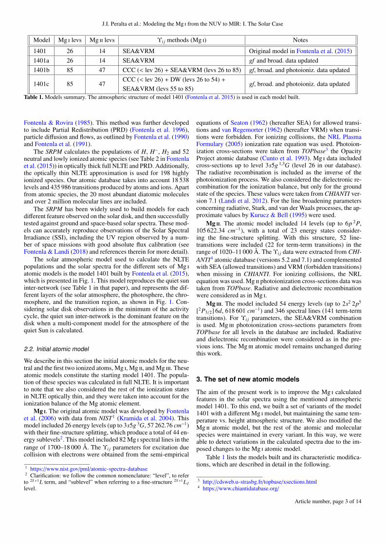
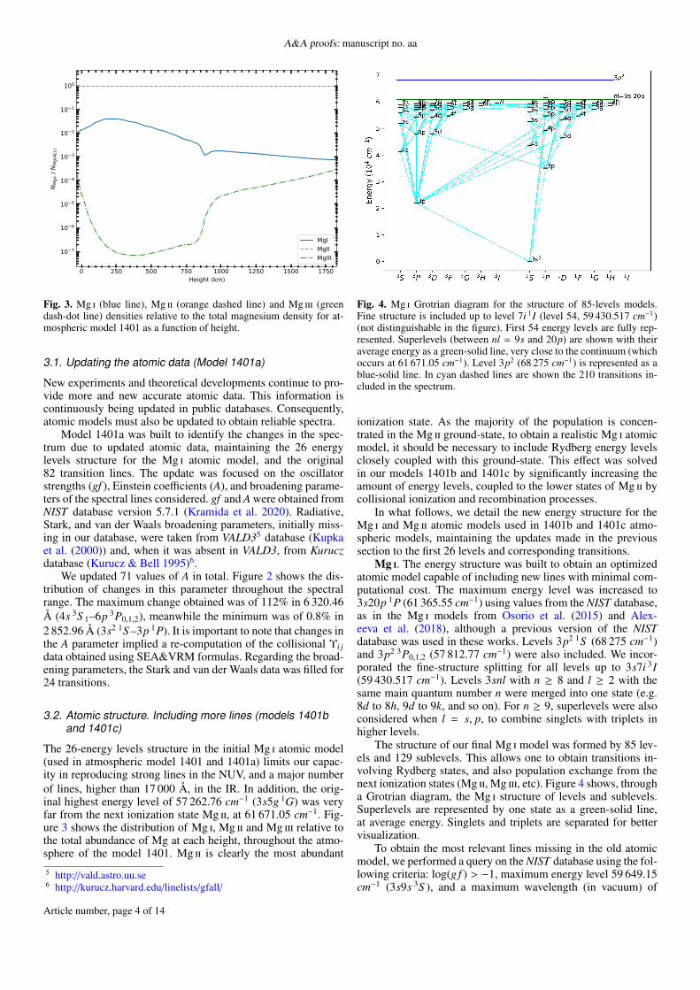
Fig. 3. Mg i (blue line), Mg ii (orange dashed line) and Mg iii (greendash-dot line) densities relative to the total magnesium density for at-mospheric model 1401 as a function of height.

3.1. Updating the atomic data (Model 1401a)

New experiments and theoretical developments continue to pro-vide more and new accurate atomic data. This information iscontinuously being updated in public databases. Consequently,atomic models must also be updated to obtain reliable spectra.

Model 1401a was built to identify the changes in the spec-trum due to updated atomic data, maintaining the 26 energylevels structure for the Mg i atomic model, and the original82 transition lines. The update was focused on the oscillatorstrengths (gf ), Einstein coefficients (A), and broadening parame-ters of the spectral lines considered. gf and A were obtained fromNIST database version 5.7.1 (Kramida et al. 2020). Radiative,Stark, and van der Waals broadening parameters, initially miss-ing in our database, were taken from VALD35 database (Kupkaet al. (2000)) and, when it was absent in VALD3, from Kuruczdatabase (Kurucz & Bell 1995)6.

We updated 71 values of A in total. Figure 2 shows the dis-tribution of changes in this parameter throughout the spectralrange. The maximum change obtained was of 112% in 6 320.46Å (4s 3S 1–6p 3P0,1,2), meanwhile the minimum was of 0.8% in2 852.96 Å (3s2 1S –3p 1P). It is important to note that changes inthe A parameter implied a re-computation of the collisional Υi jdata obtained using SEA&VRM formulas. Regarding the broad-ening parameters, the Stark and van der Waals data was filled for24 transitions.

3.2. Atomic structure. Including more lines (models 1401band 1401c)

The 26-energy levels structure in the initial Mg i atomic model(used in atmospheric model 1401 and 1401a) limits our capac-ity in reproducing strong lines in the NUV, and a major numberof lines, higher than 17 000 Å, in the IR. In addition, the orig-inal highest energy level of 57 262.76 cm−1 (3s5g 1G) was veryfar from the next ionization state Mg ii, at 61 671.05 cm−1. Fig-ure 3 shows the distribution of Mg i, Mg ii and Mg iii relative tothe total abundance of Mg at each height, throughout the atmo-sphere of the model 1401. Mg ii is clearly the most abundant

5 http://vald.astro.uu.se6 http://kurucz.harvard.edu/linelists/gfall/

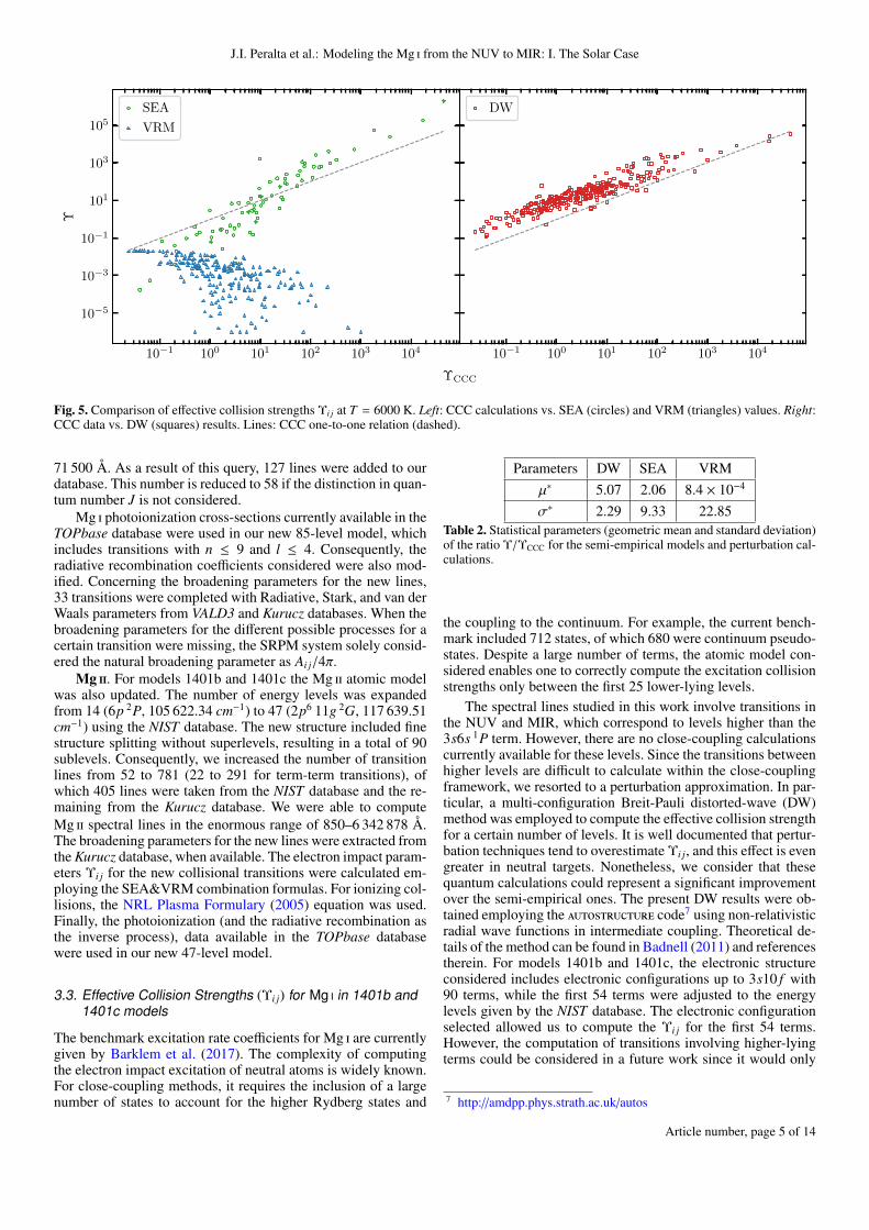
Fig. 4. Mg i Grotrian diagram for the structure of 85-levels models.Fine structure is included up to level 7i 1I (level 54, 59 430.517 cm−1)(not distinguishable in the figure). First 54 energy levels are fully rep-resented. Superlevels (between nl = 9s and 20p) are shown with theiraverage energy as a green-solid line, very close to the continuum (whichoccurs at 61 671.05 cm−1). Level 3p2 (68 275 cm−1) is represented as ablue-solid line. In cyan dashed lines are shown the 210 transitions in-cluded in the spectrum.

ionization state. As the majority of the population is concen-trated in the Mg ii ground-state, to obtain a realistic Mg i atomicmodel, it should be necessary to include Rydberg energy levelsclosely coupled with this ground-state. This effect was solvedin our models 1401b and 1401c by significantly increasing theamount of energy levels, coupled to the lower states of Mg ii bycollisional ionization and recombination processes.

In what follows, we detail the new energy structure for theMg i and Mg ii atomic models used in 1401b and 1401c atmo-spheric models, maintaining the updates made in the previoussection to the first 26 levels and corresponding transitions.

Mg i. The energy structure was built to obtain an optimizedatomic model capable of including new lines with minimal com-putational cost. The maximum energy level was increased to3s20p 1P (61 365.55 cm−1) using values from the NIST database,as in the Mg i models from Osorio et al. (2015) and Alex-eeva et al. (2018), although a previous version of the NISTdatabase was used in these works. Levels 3p2 1S (68 275 cm−1)and 3p2 3P0,1,2 (57 812.77 cm−1) were also included. We incor-porated the fine-structure splitting for all levels up to 3s7i 3I(59 430.517 cm−1). Levels 3snl with n ≥ 8 and l ≥ 2 with thesame main quantum number n were merged into one state (e.g.8d to 8h, 9d to 9k, and so on). For n ≥ 9, superlevels were alsoconsidered when l = s, p, to combine singlets with triplets inhigher levels.

The structure of our final Mg i model was formed by 85 lev-els and 129 sublevels. This allows one to obtain transitions in-volving Rydberg states, and also population exchange from thenext ionization states (Mg ii, Mg iii, etc). Figure 4 shows, througha Grotrian diagram, the Mg i structure of levels and sublevels.Superlevels are represented by one state as a green-solid line,at average energy. Singlets and triplets are separated for bettervisualization.

To obtain the most relevant lines missing in the old atomicmodel, we performed a query on the NIST database using the fol-lowing criteria: log(g f ) > −1, maximum energy level 59 649.15cm−1 (3s9s 3S ), and a maximum wavelength (in vacuum) of

Article number, page 4 of 14

J.I. Peralta et al.: Modeling the Mg i from the NUV to MIR: I. The Solar Case

10−1 100 101 102 103 104

10−5

10−3

10−1

101

103

105

Υ

SEA

VRM

10−1 100 101 102 103 104

DW

ΥCCC

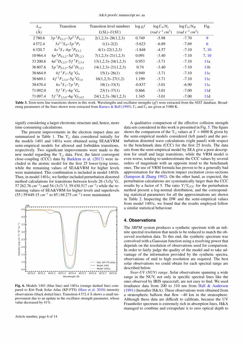
Fig. 5. Comparison of effective collision strengths Υi j at T = 6000 K. Left: CCC calculations vs. SEA (circles) and VRM (triangles) values. Right:CCC data vs. DW (squares) results. Lines: CCC one-to-one relation (dashed).

71 500 Å. As a result of this query, 127 lines were added to ourdatabase. This number is reduced to 58 if the distinction in quan-tum number J is not considered.

Mg i photoionization cross-sections currently available in theTOPbase database were used in our new 85-level model, whichincludes transitions with n ≤ 9 and l ≤ 4. Consequently, theradiative recombination coefficients considered were also mod-ified. Concerning the broadening parameters for the new lines,33 transitions were completed with Radiative, Stark, and van derWaals parameters from VALD3 and Kurucz databases. When thebroadening parameters for the different possible processes for acertain transition were missing, the SRPM system solely consid-ered the natural broadening parameter as Ai j/4π.

Mg ii. For models 1401b and 1401c the Mg ii atomic modelwas also updated. The number of energy levels was expandedfrom 14 (6p 2P, 105 622.34 cm−1) to 47 (2p6 11g 2G, 117 639.51cm−1) using the NIST database. The new structure included finestructure splitting without superlevels, resulting in a total of 90sublevels. Consequently, we increased the number of transitionlines from 52 to 781 (22 to 291 for term-term transitions), ofwhich 405 lines were taken from the NIST database and the re-maining from the Kurucz database. We were able to computeMg ii spectral lines in the enormous range of 850–6 342 878 Å.The broadening parameters for the new lines were extracted fromthe Kurucz database, when available. The electron impact param-eters Υi j for the new collisional transitions were calculated em-ploying the SEA&VRM combination formulas. For ionizing col-lisions, the NRL Plasma Formulary (2005) equation was used.Finally, the photoionization (and the radiative recombination asthe inverse process), data available in the TOPbase databasewere used in our new 47-level model.

3.3. Effective Collision Strengths (Υi j) for Mg i in 1401b and1401c models

The benchmark excitation rate coefficients for Mg i are currentlygiven by Barklem et al. (2017). The complexity of computingthe electron impact excitation of neutral atoms is widely known.For close-coupling methods, it requires the inclusion of a largenumber of states to account for the higher Rydberg states and

Parameters DW SEA VRMµ∗ 5.07 2.06 8.4 × 10−4

σ∗ 2.29 9.33 22.85Table 2. Statistical parameters (geometric mean and standard deviation)of the ratio Υ/ΥCCC for the semi-empirical models and perturbation cal-culations.

the coupling to the continuum. For example, the current bench-mark included 712 states, of which 680 were continuum pseudo-states. Despite a large number of terms, the atomic model con-sidered enables one to correctly compute the excitation collisionstrengths only between the first 25 lower-lying levels.

The spectral lines studied in this work involve transitions inthe NUV and MIR, which correspond to levels higher than the3s6s 1P term. However, there are no close-coupling calculationscurrently available for these levels. Since the transitions betweenhigher levels are difficult to calculate within the close-couplingframework, we resorted to a perturbation approximation. In par-ticular, a multi-configuration Breit-Pauli distorted-wave (DW)method was employed to compute the effective collision strengthfor a certain number of levels. It is well documented that pertur-bation techniques tend to overestimate Υi j, and this effect is evengreater in neutral targets. Nonetheless, we consider that thesequantum calculations could represent a significant improvementover the semi-empirical ones. The present DW results were ob-tained employing the autostructure code7 using non-relativisticradial wave functions in intermediate coupling. Theoretical de-tails of the method can be found in Badnell (2011) and referencestherein. For models 1401b and 1401c, the electronic structureconsidered includes electronic configurations up to 3s10 f with90 terms, while the first 54 terms were adjusted to the energylevels given by the NIST database. The electronic configurationselected allowed us to compute the Υi j for the first 54 terms.However, the computation of transitions involving higher-lyingterms could be considered in a future work since it would only

7 http://amdpp.phys.strath.ac.uk/autos

Article number, page 5 of 14

A&A proofs: manuscript no. aa

λvac Transition Transition level numbers log g f log Γ4/Ne log Γ6/NH Fig.(Å) L(SL)–U(SU) (rad s−1 cm3) (rad s−1 cm3)

2 780.6 3p 3P0,1,2–3p2 3P0,1,2 2(1,2,3)–28(1,2,3) 0.749 -5.98 -7.70 94 572.4 3s2 1S 0–3p 3P1 1(1)–2(2) -5.623 -6.89 -7.69 66 320.7 4s 3S 1–6p 3P0,1,2 4(1)–22(1,2,3) -1.848 -4.57 -7.10 7, 10

10 964.4 4p 3P0,1,2–5d 3D1,2,3 7(1,2,3)–21(1,2,3) 0.091 -3.40 -7.10 7, 1033 200.6 4d 3D1,2,3–5 f 3F2,3,4 13(1,2,3)–24(1,2,3) 0.953 -3.71 -7.10 11a36 807.6 5p 3P0,1,2–5d 3D1,2,3 14(1,2,3)–21(1,2,3) 0.74 -3.40 -7.10 11b38 664.9 4 f 1F3–5g 1G4 15(1)–26(1) 0.949 -3.71 -7.10 11c38 669.1 4 f 3F2,3,4–5g 3G3,4 16(1,2,3)–27(1,2) 1.199 -3.71 -7.10 11c38 670.4 6s 3S 1–7p 3P2 18(1)–33(3) -0.837 -3.01 -6.90 11c71 092.0 5 f 1F3–6g 1G4 23(1)–37(1) 0.866 -3.01 -7.00 11d71 097.4 5 f 3F2,3,4–6g 3G3,4,5 24(1,2,3)–38(1,2,3) 1.345 -3.01 -7.00 11d

Table 3. Term-term line transitions shown in this work. Wavelengths and oscillator strengths (gf ) were extracted from the NIST database. Broad-ening parameters of the lines shown were extracted from Kurucz & Bell (1995). Γ4 and Γ6 are given at 5 000 K.

signify considering a larger electronic structure and, hence, moretime-consuming calculations.

The present improvements in the electron impact data aresummarized in Table 1. The Υi j data considered initially forthe models 1401 and 1401a were obtained using SEA&VRMsemi-empirical models for allowed and forbidden transitions,respectively. Two significant improvements were made to thenew model regarding the Υi j data. First, the latest convergentclose-coupling (CCC) data by Barklem et al. (2017) were in-cluded in the atomic model for the first 25 lower-lying terms,while the remaining values of SEA&VRM for higher levelswere maintained. This combination is included in model 1401b.Then, in model 1401c, we further included perturbation distortedmethod calculations for transitions between levels 26 (3s5g 1G,57 262.76 cm−1) and 54 (3s7i 1I, 59 430.517 cm−1) while the re-maining values of SEA&VRM for higher levels and superlevels(55 | 59 649.15 cm−1 to 85 | 68 275 cm−1) were maintained.

4572.0 4572.1 4572.2 4572.3 4572.4 4572.5 4572.6 4572.7 4572.8Wavelength (Å)

0.5

1.0

1.5

2.0

2.5

3.0

3.5

4.0

4.5

Inte

nsity

(erg

cm2 s

1 Å1 s

r1 )

1e6

Obs: KP-FTS atlasModel 1401Model 1401a

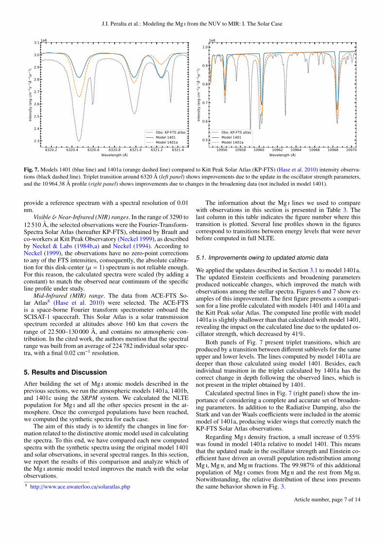
Fig. 6. Models 1401 (blue line) and 1401a (orange dashed line) com-pared to Kitt Peak Solar Atlas (KP-FTS) (Hase et al. 2010) intensityobservations (black dotted line). Transition 4 572.4 Å shows a small im-provement due to an update in the oscillator strength parameter, whosevalue decreased by 41%.

A qualitative comparison of the effective collision strengthdata sets considered in this work is presented in Fig. 5. The figureshows the comparison of the Υi j values at T = 6000 K given bythe semi-empirical models considered (left panel) and the per-turbation distorted wave calculations (right panel) with respectto the benchmark data (CCC) for the first 25 levels. The datasets from the semi-empirical model by SEA give a poor descrip-tion for small and large transitions, while the VRM model iseven worse, tending to underestimate the CCC values by severalorders of magnitude with an opposite trend to the benchmarkones. The use of VRM formula has proven to be a generally badapproximation for the electron impact excitation cross-sections(Sampson & Zhang 1992). On the other hand, as expected, theperturbation calculations are systematically larger than the CCCresults by a factor of 5. The ratio Υ/ΥCCC for the perturbationmethod present a log-normal distribution, and the correspond-ing statistical parameters for all the approximations are shownin Table 2. Inspecting the DW and the semi-empirical valuesfrom model 1401c, we found that the results employed followa similar statistical behaviour.

4. Observations

The SRPM system produces a synthetic spectrum with an infi-nite spectral resolution that needs to be reduced to match the ob-served resolution data. To this end, the synthetic spectrum wasconvolved with a Gaussian function using a resolving power thatdepends on the resolution of observations used for comparison.In order to fairly judge the quality of the model and to take ad-vantage of the information provided by the synthetic spectra,observations of mid to high resolution are required. The bestsolar observations we could obtain for each spectral range aredescribed below.

Near-UV (NUV) range. Solar observations spanning a widerange in the NUV, not only in specific spectral lines like theones observed by IRIS spacecraft, are not easy to find. We usedirradiance data from 200 to 310 nm from Hall & Anderson(1991) (hereafter H&A). These observations were obtained froma stratospheric balloon that flew ∼40 km in the stratosphere.Although these data are difficult to calibrate, because the UVFraunhofer spectrum is extremely rich in absorption lines, H&Amanaged to combine and extrapolate it to zero optical depth to

Article number, page 6 of 14

J.I. Peralta et al.: Modeling the Mg i from the NUV to MIR: I. The Solar Case

6320.2 6320.4 6320.6 6320.8 6321.0 6321.2 6321.4Wavelength (Å)

2.3

2.4

2.5

2.6

2.7

2.8

2.9

3.0

3.1

Inte

nsity

(erg

cm2 s

1 Å1 s

r1 )

1e6

Obs: KP-FTS atlasModel 1401Model 1401a

10956 10958 10960 10962 10964 10966 10968 10970Wavelength (Å)

0.5

0.6

0.7

0.8

0.9

1.0

Inte

nsity

(erg

cm2 s

1 Å1 s

r1 )

1e6

Obs: KP-FTS atlasModel 1401Model 1401a

Fig. 7. Models 1401 (blue line) and 1401a (orange dashed line) compared to Kitt Peak Solar Atlas (KP-FTS) (Hase et al. 2010) intensity observa-tions (black dashed line). Triplet transition around 6320 Å (left panel) shows improvements due to the update in the oscillator strength parameters,and the 10 964.38 Å profile (right panel) shows improvements due to changes in the broadening data (not included in model 1401).

provide a reference spectrum with a spectral resolution of 0.01nm.

Visible&Near-Infrared (NIR) ranges. In the range of 3290 to12 510 Å, the selected observations were the Fourier-Transform-Spectra Solar Atlas (hereafter KP-FTS), obtained by Brault andco-workers at Kitt Peak Observatory (Neckel 1999), as describedby Neckel & Labs (1984b,a) and Neckel (1994). According toNeckel (1999), the observations have no zero-point correctionsto any of the FTS intensities, consequently, the absolute calibra-tion for this disk-center (µ = 1) spectrum is not reliable enough.For this reason, the calculated spectra were scaled (by adding aconstant) to match the observed near continuum of the specificline profile under study.

Mid-Infrared (MIR) range. The data from ACE-FTS So-lar Atlas8 (Hase et al. 2010) were selected. The ACE-FTSis a space-borne Fourier transform spectrometer onboard theSCISAT-1 spacecraft. This Solar Atlas is a solar transmissionspectrum recorded at altitudes above 160 km that covers therange of 22 500–130 000 Å, and contains no atmospheric con-tribution. In the cited work, the authors mention that the spectralrange was built from an average of 224 782 individual solar spec-tra, with a final 0.02 cm−1 resolution.

5. Results and Discussion

After building the set of Mg i atomic models described in theprevious sections, we run the atmospheric models 1401a, 1401b,and 1401c using the SRPM system. We calculated the NLTEpopulation for Mg i and all the other species present in the at-mosphere. Once the converged populations have been reached,we computed the synthetic spectra for each case.

The aim of this study is to identify the changes in line for-mation related to the distinctive atomic model used in calculatingthe spectra. To this end, we have compared each new computedspectra with the synthetic spectra using the original model 1401and solar observations, in several spectral ranges. In this section,we report the results of this comparison and analyze which ofthe Mg i atomic model tested improves the match with the solarobservations.8 http://www.ace.uwaterloo.ca/solaratlas.php

The information about the Mg i lines we used to comparewith observations in this section is presented in Table 3. Thelast column in this table indicates the figure number where thistransition is plotted. Several line profiles shown in the figurescorrespond to transitions between energy levels that were neverbefore computed in full NLTE.

5.1. Improvements owing to updated atomic data

We applied the updates described in Section 3.1 to model 1401a.The updated Einstein coefficients and broadening parametersproduced noticeable changes, which improved the match withobservations among the stellar spectra. Figures 6 and 7 show ex-amples of this improvement. The first figure presents a compari-son for a line profile calculated with models 1401 and 1401a andthe Kitt Peak solar Atlas. The computed line profile with model1401a is slightly shallower than that calculated with model 1401,revealing the impact on the calculated line due to the updated os-cillator strength, which decreased by 41%.

Both panels of Fig. 7 present triplet transitions, which areproduced by a transition between different sublevels for the sameupper and lower levels. The lines computed by model 1401a aredeeper than those calculated using model 1401. Besides, eachindividual transition in the triplet calculated by 1401a has thecorrect change in depth following the observed lines, which isnot present in the triplet obtained by 1401.

Calculated spectral lines in Fig. 7 (right panel) show the im-portance of considering a complete and accurate set of broaden-ing parameters. In addition to the Radiative Damping, also theStark and van der Waals coefficients were included in the atomicmodel of 1401a, producing wider wings that correctly match theKP-FTS Solar Atlas observations.

Regarding Mg i density fraction, a small increase of 0.55%was found in model 1401a relative to model 1401. This meansthat the updated made in the oscillator strength and Einstein co-efficient have driven an overall population redistribution amongMg i, Mg ii, and Mg iii fractions. The 99.987% of this additionalpopulation of Mg i comes from Mg ii and the rest from Mg iii.Notwithstanding, the relative distribution of these ions presentsthe same behavior shown in Fig. 3.

Article number, page 7 of 14

A&A proofs: manuscript no. aa

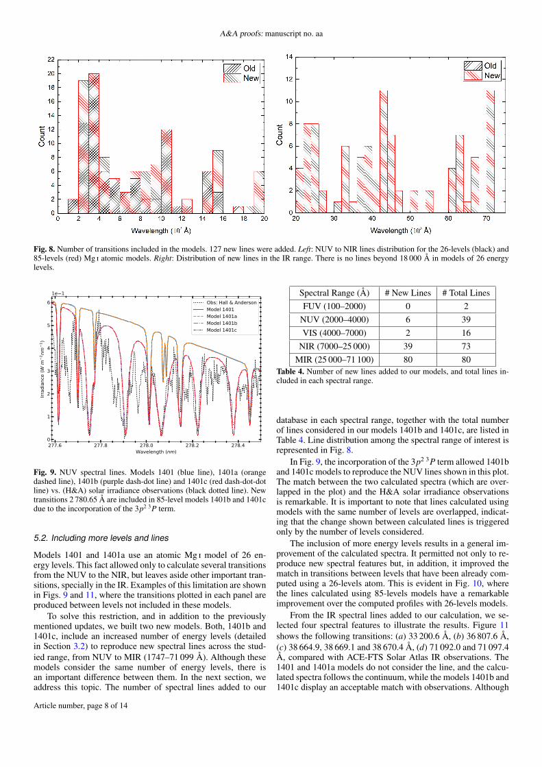
Fig. 8. Number of transitions included in the models. 127 new lines were added. Left: NUV to NIR lines distribution for the 26-levels (black) and85-levels (red) Mg i atomic models. Right: Distribution of new lines in the IR range. There is no lines beyond 18 000 Å in models of 26 energylevels.

277.6 277.8 278.0 278.2 278.4Wavelength (nm)

0

1

2

3

4

5

6

Irrad

ianc

e (W

m2 n

m1 )

1e 1Obs: Hall & AndersonModel 1401Model 1401aModel 1401bModel 1401c

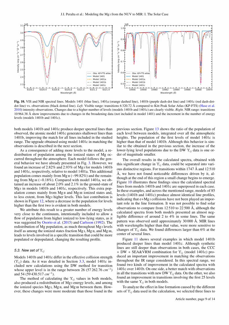
Fig. 9. NUV spectral lines. Models 1401 (blue line), 1401a (orangedashed line), 1401b (purple dash-dot line) and 1401c (red dash-dot-dotline) vs. (H&A) solar irradiance observations (black dotted line). Newtransitions 2 780.65 Å are included in 85-level models 1401b and 1401cdue to the incorporation of the 3p2 3P term.

5.2. Including more levels and lines

Models 1401 and 1401a use an atomic Mg i model of 26 en-ergy levels. This fact allowed only to calculate several transitionsfrom the NUV to the NIR, but leaves aside other important tran-sitions, specially in the IR. Examples of this limitation are shownin Figs. 9 and 11, where the transitions plotted in each panel areproduced between levels not included in these models.

To solve this restriction, and in addition to the previouslymentioned updates, we built two new models. Both, 1401b and1401c, include an increased number of energy levels (detailedin Section 3.2) to reproduce new spectral lines across the stud-ied range, from NUV to MIR (1747–71 099 Å). Although thesemodels consider the same number of energy levels, there isan important difference between them. In the next section, weaddress this topic. The number of spectral lines added to our

Spectral Range (Å) # New Lines # Total LinesFUV (100–2000) 0 2

NUV (2000–4000) 6 39VIS (4000–7000) 2 16

NIR (7000–25 000) 39 73MIR (25 000–71 100) 80 80

Table 4. Number of new lines added to our models, and total lines in-cluded in each spectral range.

database in each spectral range, together with the total numberof lines considered in our models 1401b and 1401c, are listed inTable 4. Line distribution among the spectral range of interest isrepresented in Fig. 8.

In Fig. 9, the incorporation of the 3p2 3P term allowed 1401band 1401c models to reproduce the NUV lines shown in this plot.The match between the two calculated spectra (which are over-lapped in the plot) and the H&A solar irradiance observationsis remarkable. It is important to note that lines calculated usingmodels with the same number of levels are overlapped, indicat-ing that the change shown between calculated lines is triggeredonly by the number of levels considered.

The inclusion of more energy levels results in a general im-provement of the calculated spectra. It permitted not only to re-produce new spectral features but, in addition, it improved thematch in transitions between levels that have been already com-puted using a 26-levels atom. This is evident in Fig. 10, wherethe lines calculated using 85-levels models have a remarkableimprovement over the computed profiles with 26-levels models.

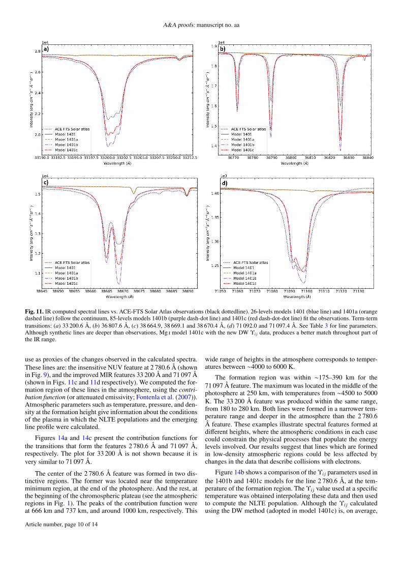
From the IR spectral lines added to our calculation, we se-lected four spectral features to illustrate the results. Figure 11shows the following transitions: (a) 33 200.6 Å, (b) 36 807.6 Å,(c) 38 664.9, 38 669.1 and 38 670.4 Å, (d) 71 092.0 and 71 097.4Å, compared with ACE-FTS Solar Atlas IR observations. The1401 and 1401a models do not consider the line, and the calcu-lated spectra follows the continuum, while the models 1401b and1401c display an acceptable match with observations. Although

Article number, page 8 of 14

J.I. Peralta et al.: Modeling the Mg i from the NUV to MIR: I. The Solar Case

6320.2 6320.4 6320.6 6320.8 6321.0 6321.2 6321.4Wavelength (Å)

2.3

2.4

2.5

2.6

2.7

2.8

2.9

3.0

3.1

Inte

nsity

(erg

cm2 s

1 Å1 s

r1 )

1e6

Obs: KP-FTS atlasModel 1401Model 1401aModel 1401bModel 1401c

10956 10958 10960 10962 10964 10966 10968 10970Wavelength (Å)

0.5

0.6

0.7

0.8

0.9

1.0

Inte

nsity

(erg

cm2 s

1 Å1 s

r1 )

1e6

Obs: KP-FTS atlasModel 1401Model 1401aModel 1401bModel 1401c

Fig. 10. VIS and NIR spectral lines. Models 1401 (blue line), 1401a (orange dashed line), 1401b (purple dash-dot line) and 1401c (red dash-dot-dot line) vs. observations (black dotted line). Left. Visible range: transitions 6 320.72 Å compared to Kitt Peak Solar Atlas (KP-FTS) (Hase et al.2010) intensity observations. Changes due to a higher number of levels (models 1401b and 1401c) are clearly visible. Right. NIR range: transitions10 964.38 Å show improvements due to changes in the broadening data (not included in model 1401) and the increment in the number of energylevels (models 1401b and 1401c).

both models 1401b and 1401c produce deeper spectral lines thanobserved, the atomic model 1401c generates shallower lines than1401b, improving the match for all lines included in the studiedrange. The upgrade obtained using model 1401c in matching theobservations is described in the next section.

As a consequence of adding more levels to the model, a re-distribution of population among the ionized states of Mg oc-curred throughout the atmosphere. Each model follows the gen-eral behavior we have already presented in Fig. 3. However, wefound an increase of 2.82% and 2.93% of Mg i for models 1401band 1401c, respectively, relative to model 1401a. This additionalpopulation comes mainly from Mg ii (∼99.82%) and the remain-ing from Mg iii (∼0.18%). Compared with model 1401a, we ob-tained an increase of about 2.0% and 2.1% in the ground-state ofMg i in models 1401b and 1401c, respectively. This extra pop-ulation comes mainly from Mg ii and Mg iii ionized states and,to less extent, from Mg i higher levels. This last contribution isshown in Figure 12, where a decrease in the population for levelshigher than the first two is evident in both models.

We attribute this result to a greater number of energy levelsvery close to the continuum, intentionally included to allow aflow of population from higher ionized to low-lying states, as itwas suggested by Osorio et al. (2015) and Carlsson (1992). Theredistribution of Mg population, as much throughout Mg i levelsitself as among the ionized states fraction Mg i, Mg ii, and Mg iii,leads to levels involved in a specific transition that could be morepopulated or depopulated, changing the resulting profile.

5.3. New set of Υi j

Models 1401b and 1401c differ in the effective collision strength(Υi j) data. As it was detailed in Section 3.3, model 1401c in-cluded new calculations using the DW method for transitionwhose upper level is in the range between 26 (57 262.76 cm−1)and 54 (59 430.517 cm−1).

The method of calculating the Υi j values in both models,also produced a redistribution of Mg i energy levels, and amongthe ionized species Mg i, Mg ii, and Mg iii between them. How-ever, these changes were more moderate than those found in the

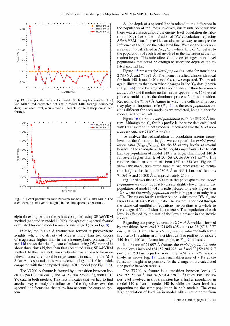
previous section. Figure 13 shows the ratio of the population ofeach level between models, integrated over all the atmosphericheights. The population of the first levels of model 1401c ishigher than that of model 1401b. Although this behavior is sim-ilar to the obtained in the previous section, the increase of thelower-lying level populations due to the DW Υi j data is one or-der of magnitude smaller.

The overall results in the calculated spectra, obtained withthis significant change in Υi j data, could be separated into vari-ous distinctive regions. For transitions within 1747 Å and 12 510Å, we have not found noticeable differences driven by it, al-though at the end of this region a small change begins to emerge.Figure 10 illustrates these findings since the calculated spectrallines from models 1401b and 1401c are superposed in each case.In these examples, and across the mentioned range, models of 85levels (1401b and 1401c) produce almost identical line profiles,indicating that e+Mg i collisions have not been played an impor-tant role in the line formation. It was not possible to find solarobservations to compare from 12 510 to 22 500 Å, although thecalculated spectra from both models presented an almost neg-ligible difference of around 2 to 4% in some lines. The samepattern was observed until approximately 30 000 Å. MIR lineswith wavelengths higher than that value, were more sensitive tochanges of Υi j data. We found differences larger than 6% at thecenter of several lines.

Figure 11 shows several examples in which model 1401bproduced deeper lines than model 1401c. Although syntheticlines are still deeper than observations in both cases, the CCC+ DW + SEA&VRM combination for Υi j (model 1401c) pro-duced an important improvement in matching the observationsthroughout the IR range considered. In this spectral range, wefound two kinds of improvement in the calculated spectra with1401c over 1401b. On one side, a better match with observationsin all the transitions with new DW Υi j data. On the other, we alsofound an improvement in transitions involving the first 25 levelswith the same Υi j in both models.

To analyze the effect in line formation caused by the differentsets of Υi j data used in the calculation, we selected three lines to

Article number, page 9 of 14

A&A proofs: manuscript no. aa

Fig. 11. IR computed spectral lines vs. ACE-FTS Solar Atlas observations (black dottedline). 26-levels models 1401 (blue line) and 1401a (orangedashed line) follow the continuum, 85-levels models 1401b (purple dash-dot line) and 1401c (red dash-dot-dot line) fit the observations. Term-termtransitions: (a) 33 200.6 Å, (b) 36 807.6 Å, (c) 38 664.9, 38 669.1 and 38 670.4 Å, (d) 71 092.0 and 71 097.4 Å. See Table 3 for line parameters.Although synthetic lines are deeper than observations, Mg i model 1401c with the new DW Υi j data, produces a better match throughout part ofthe IR range.

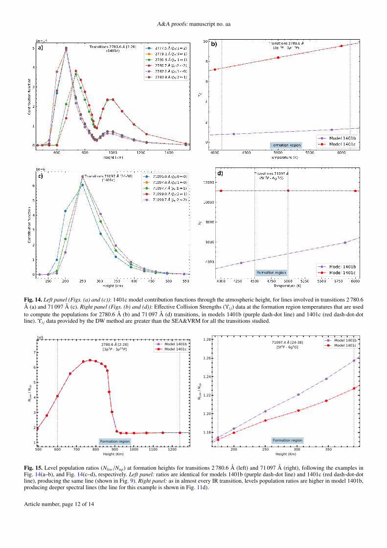
use as proxies of the changes observed in the calculated spectra.These lines are: the insensitive NUV feature at 2 780.6 Å (shownin Fig. 9), and the improved MIR features 33 200 Å and 71 097 Å(shown in Figs. 11c and 11d respectively). We computed the for-mation region of these lines in the atmosphere, using the contri-bution function (or attenuated emissivity; Fontenla et al. (2007)).Atmospheric parameters such as temperature, pressure, and den-sity at the formation height give information about the conditionsof the plasma in which the NLTE populations and the emergingline profile were calculated.

Figures 14a and 14c present the contribution functions forthe transitions that form the features 2 780.6 Å and 71 097 Å,respectively. The plot for 33 200 Å is not shown because it isvery similar to 71 097 Å.

The center of the 2 780.6 Å feature was formed in two dis-tinctive regions. The former was located near the temperatureminimum region, at the end of the photosphere. And the rest, atthe beginning of the chromospheric plateau (see the atmosphericregions in Fig. 1). The peaks of the contribution function wereat 666 km and 737 km, and around 1000 km, respectively. This

wide range of heights in the atmosphere corresponds to temper-atures between ∼4000 to 6000 K.

The formation region was within ∼175–390 km for the71 097 Å feature. The maximum was located in the middle of thephotosphere at 250 km, with temperatures from ∼4500 to 5000K. The 33 200 Å feature was produced within the same range,from 180 to 280 km. Both lines were formed in a narrower tem-perature range and deeper in the atmosphere than the 2 780.6Å feature. These examples illustrate spectral features formed atdifferent heights, where the atmospheric conditions in each casecould constrain the physical processes that populate the energylevels involved. Our results suggest that lines which are formedin low-density atmospheric regions could be less affected bychanges in the data that describe collisions with electrons.

Figure 14b shows a comparison of the Υi j parameters used inthe 1401b and 1401c models for the line 2 780.6 Å, at the tem-perature of the formation region. The Υi j value used at a specifictemperature was obtained interpolating these data and then usedto compute the NLTE population. Although the Υi j calculatedusing the DW method (adopted in model 1401c) is, on average,

Article number, page 10 of 14

J.I. Peralta et al.: Modeling the Mg i from the NUV to MIR: I. The Solar Case

0 5 10 15 20 25Level Number

0.995

1.000

1.005

1.010

1.015

1.020

Nm

odel

/ N

1401

a

Model 1401aModel 1401bModel 1401c

Fig. 12. Level population ratio for model 1401b (purple connected dots)and 1401c (red connected dots) with model 1401 (orange connecteddots). For each level, a sum over all heights in the atmosphere is per-formed.

0 20 40 60 80Level Number

0.9998

1.0000

1.0002

1.0004

1.0006

1.0008

1.0010

1.0012

N14

01c /

N14

01b

Model 1401bModel 1401c

Fig. 13. Level population ratio between models 1401c and 1401b. Foreach level, a sum over all heights in the atmosphere is performed.

eight times higher than the values computed using SEA&VRMmethod (adopted in model 1401b), the synthetic spectral featurecalculated for each model remained unchanged (see in Fig. 9).

Instead, the 71 097 Å feature was formed at photosphericheights, where the density of Mg i is more than two ordersof magnitude higher than in the chromospheric plateau. Fig-ure 14d shows that the Υi j data calculated using DW method isabout three times higher than that computed using SEA&VRMmethod. In this case, collisions with electron appear to be morerelevant since a remarkable improvement in matching the ACESolar Atlas spectral lines was reached using the 1401c model,compared with that computed using 1401b model (see Fig. 11d).

The 33 200 Å feature is formed by a transition between lev-els 13 (54 192.256 cm−1) and 24 (57 204.228 cm−1), with CCCΥi j data in both models. This fact indicates that we had to findanother way to study the influence of the Υi j values over thespectral line formation that takes into account the coupled sys-tem.

As the depth of a spectral line is related to the difference inthe population of the levels involved, our results point out thatthere was a change among the energy level population distribu-tion of Mg i due to the inclusion of DW calculations replacingSEA&VRM data. It provides an alternative way to analyze theinfluence of the Υi j on the calculated line. We used the level pop-ulation ratio calculated as Nlow/Nup, where Nlow or Nup refers tothe populations of each level involved in the transition at the for-mation height. This ratio allowed to detect changes in the levelpopulations that could be enough to affect the depth of the re-lated spectral line.

Figure 15 presents the level population ratio for transitions2 780.6 Å and 71 097 Å. The former resulted almost identicalfor both 1401b and 1401c models, as we expected. This resultagain illustrates that even when changes in the Υi j data (shownin Fig. 14b) could be large, it has no influence in their level popu-lation ratio and therefore neither in the spectral line. Collisionalprocess could not be the dominant process for this transition.Regarding the 71 097 Å feature in which the collisional processmay play an important role (Fig. 14d), the level population ra-tio is different for each model as we predicted, being higher formodel 1401b than 1401c.

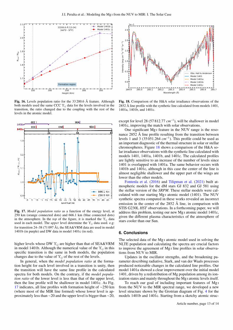
Figure 16 shows the level population ratio for 33 200 Å fea-ture. Although the Υi j for this profile is the same data calculatedwith CCC method in both models, it behaved like the level pop-ulations ratio for 71 097 Å profile.

To analyze the redistribution of population among energylevels at the formation height, we computed the model popu-lation ratio (N1401c/N1401b) for the 85 energy levels, at severalheights in the atmosphere. In the height range from ∼175 to 550km, the population of model 1401c is larger than model 1401bfor levels higher than level 20 (5d 1D, 56 308.381 cm−1). Thisratio reaches a maximum of about 12% at 350 km. Figure 17shows the model population ratio at two representative forma-tion heights, for feature 2 780.6 Å at 666.1 km, and features71 097 Å and 33 200 Å at approximately 250 km.

Fig. 17 shows that at 250 km in the photosphere, the modelpopulation ratio for the first levels are slightly lower than 1. Thepopulation of model 1401c is redistributed to levels higher than∼20, where the model population ratio is bigger than unity in a∼7%. The reason for this redistribution is due to the DW Υi j arelarger than SEA&VRM Υi j data. The system is coupled throughthe statistical equilibrium equations, responding as a whole tothe change of Υi j collisional parameters. The population of eachlevel is affected by the rest of the levels present in the atomicmodel.

Regarding our proxy features, the 2 780.6 Å profile is formedby transitions from level 2 (21 850.405 cm−1) to 28 (57 812.77cm−1) at 666.1 km. The model population ratio for both levelsis close to 1 resulting in almost identical line profiles for models1401b and 1401c at formation height, as Fig. 9 indicates.

In the case of 71 097 Å feature, the model population ratiofor the levels involved (24 | 57 204.228 cm−1 and 38 | 59 430.517cm−1) at 250 km, departes from unity ∼6%, and ∼7% respec-tively, as shows Fig. 17. This small difference of ∼1% at theformation height is responsible for the change on the calculatedline profile between models.

The 33 200 Å feature is a transition between levels 13(54 192.256 cm−1) and 24 (57 204.228 cm−1) at 250 km. The up-per level involved in this transition has a higher population inmodel 1401c than in model 1401b, while the lower level hasapproximated the same population in both models. The extraMg i population of level 24 in model 1401c, could come from

Article number, page 11 of 14

A&A proofs: manuscript no. aa

Fig. 14. Left panel (Figs. (a) and (c)): 1401c model contribution functions through the atmospheric height, for lines involved in transitions 2 780.6Å (a) and 71 097 Å (c). Right panel (Figs. (b) and (d)): Effective Collision Strengths (Υi j) data at the formation region temperatures that are usedto compute the populations for 2780.6 Å (b) and 71 097 Å (d) transitions, in models 1401b (purple dash-dot line) and 1401c (red dash-dot-dotline). Υi j data provided by the DW method are greater than the SEA&VRM for all the transitions studied.

500 600 700 800 900 1000 1100 1200Height (Km)

1

2

3

4

5

6

7

NLo

w /

NU

p

1e5

Formation region

2780.6 Å [2-28][3p3P - 3p23P]

Model 1401bModel 1401c

200 250 300 350Height (Km)

1.18

1.20

1.22

1.24

1.26

1.28

NLo

w /

NU

p

Formation region

71097.4 Å [24-38][5f3F - 6g3G]

Model 1401bModel 1401c

Fig. 15. Level population ratios (Nlow/Nup) at formation heights for transitions 2 780.6 Å (left) and 71 097 Å (right), following the examples inFig. 14(a–b), and Fig. 14(c–d), respectively. Left panel: ratios are identical for models 1401b (purple dash-dot line) and 1401c (red dash-dot-dotline), producing the same line (shown in Fig. 9). Right panel: as in almost every IR transition, levels population ratios are higher in model 1401b,producing deeper spectral lines (the line for this example is shown in Fig. 11d).

Article number, page 12 of 14

J.I. Peralta et al.: Modeling the Mg i from the NUV to MIR: I. The Solar Case

150 200 250 300 350Height (Km)

1.7

1.8

1.9

2.0

2.1

NLo

w /

NU

p

Formation region

33200.6 Å [13-24][4d3D - 5f3F]

Model 1401bModel 1401c

Fig. 16. Levels population ratio for the 33 200.6 Å feature. Althoughboth models used the same CCC Υi j data for the levels involved in thetransition, the ratio changed due to the coupling with the rest of thelevels in the atomic model.

Fig. 17. Model population ratio as a function of the energy level, at250 km (orange connected dots) and 666.1 km (blue connected dots)in the atmosphere. In the top of the figure, it is marked the Υi j dataused in each model. The upper level determine the Υi j data used. e.g:for transition 24–38 (71 097 Å), the SEA&VRM data are used in model1401b (in purple) and DW data in model 1401c (in red).

higher levels whose DW Υi j are higher than that of SEA&VRMin model 1401b. Although the numerical value of the Υi j in thisspecific transition is the same in both models, the populationchanges due to the value of Υi j of the rest of the levels.

In general, when the model population ratio at the forma-tion height for each level involved in a transition is unity, thenthe transition will have the same line profile in the calculatedspectra for both models. On the contrary, if the model popula-tion ratio of the lower level is less than that of the upper level,then the line profile will be shallower in model 1401c. As Fig.17 indicates, all line profiles with formation height of ∼250 km(where most of the MIR line formed) whose lower level is ap-proximately less than ∼20 and the upper level is bigger than ∼20,

284.9 285.0 285.1 285.2 285.3 285.4 285.5 285.6 285.7Wavelength (Å)

0.0

0.5

1.0

1.5

2.0

2.5

Inte

nsity

(erg

cm2 s

1 Å1 s

r1 )

1e 1

Obs: Hall & AndersonModel 1401Model 1401aModel 1401bModel 1401c

Fig. 18. Comparison of the H&A solar irradiance observations of the2852 Å line profile with the synthetic line calculated from models 1401,1401a, 1401b, and 1401c.

except for level 28 (57 812.77 cm−1), will be shallower in model1401c, improving the match with solar observations.

One significant Mg i feature in the NUV range is the reso-nance 2852 Å line profile resulting from the transition betweenlevels 1 and 3 (35 051.264 cm−1). This profile could be used asan important diagnostic of the thermal structure in solar or stellarchromospheres. Figure 18 shows a comparison of the H&A so-lar irradiance observations with the synthetic line calculated withmodels 1401, 1401a, 1401b, and 1401c. The calculated profilesare lightly sensitive to an increase of the number of levels since1401 is overlapped with 1401a. The same behavior occurs with1401b and 1401c, although in this case the center of the line isalmost negligible shallower and the upper part of the wings arelower than the other models.

Fontenla et al. (2016) and Tilipman et al. (2021) built at-mospheric models for the dM stars GJ 832 and GJ 581 usingthe stellar version of the SRPM. These stellar models were cal-culated with our starting Mg i atomic model (1401). The NUVsynthetic spectra computed in these works revealed an incorrectemission in the center of the 2852 Å line, in comparison withSTIS G230L HST observations. In a forthcoming paper, we willaddress this problem, testing our new Mg i atomic model 1401c,given the different plasma characteristics of the atmosphere ofstars cooler than our Sun.

6. Conclusions

The selected data of the Mg i atomic model used in solving theNLTE population and calculating the spectra are crucial factorsto improve the agreement of Mg i line profiles in solar observa-tions from NUV to MIR.

Updates in the oscillator strengths, and the broadening pa-rameter describing radiative, Stark, and van der Waals processesproduced noticeable changes in the calculated line profiles. Ourmodel 1401a showed a clear improvement over the initial model1401, driven by a redistribution of Mg population among its ion-ization states and mainly throughout the Mg i atomic levels itself.

To reach our goal of including important features of Mg ifrom the NUV to the MIR spectral range, we developed a newlevel structure shown by the Grotrian diagram of Fig. 4 for themodels 1401b and 1401c. Starting from a sketchy atomic struc-

Article number, page 13 of 14

A&A proofs: manuscript no. aa

ture of 26 levels, we ended with a robust structure of 85 levelscapable of reproducing a long list of transitions, many of whichhave never been calculated in NLTE and studied in detail before.

Regarding the effective collision strength Υi j parameter, wemade use of the latest CCC calculation by Barklem et al. (2017)for the first 25 levels. For the following levels, we consid-ered the widely used formulation of SEA&VRM (yielding themodel 1401b). To find a better agreement in the line profiles, weperformed a new calculation for these parameters from levels26 (57 262.76 cm−1) to 54 (59 430.517 cm−1) with the multi-configuration Breit–Pauli distorted–wave (DW) method (usedby model 1401c). This method has seldom been used in stellarastrophysics. We found an additional improvement to that ob-tained updating and expanding the level structure due to the DWΥi j calculation. The synthetic spectra obtained using the model1401c reached a better agreement with solar observations fromNUV to MIR (1747–71 099 Å) than the other models consid-ered. Nevertheless, the observed profiles are still shallower thanthe calculated lines.

These results open new challenges for future work. We willcontinue improving the calculation of the Υi j data from level 55to 85 using the DW method. The inclusion of this new data in thestatistical equilibrium equations could produce a redistributionof the Mg population similar to that obtained in the present work.It could imply even shallower line profiles than those obtainedwith the model 1401c, potentially achieving an excellent matchwith solar observations.

The DW method has shown to be a better alternative toSEA&VRM for calculating the Υi j parameters of Mg i whenclose-coupling methods are impracticable or data are not avail-able. We suggest that its application to other atomic speciesshould be a more reliable option to semi-empirical calculations.

As the effective collision strength parameters depend on thetemperature, the plasma characteristics of the region in whicha transition is formed determine the NLTE population and theresulting line profile. Forthcoming work will mainly cover theNLTE Mg i line formation in stars with different spectral types,with a special interest in stars cooler than our Sun with planetsin its habitable zone.Acknowledgements. We wish to sincerely thank to Dr. Jeffrey Linsky for hisdetailed revision of our manuscript since it has helped us improve our work.This work has made use of the VALD database, operated at Uppsala University,the Institute of Astronomy RAS in Moscow, and the University of Vienna. Weacknowledge to 1995 Atomic Line Data (R.L. Kurucz and B. Bell) Kurucz CD-ROM No. 23. Cambridge, Mass.: Smithsonian Astrophysical Observatory.

ReferencesAlexeeva, S., Ryabchikova, T., Mashonkina, L., & Hu, S. 2018, ApJ, 866, 153Badnell, N. R. 2011, Computer Physics Communications, 182, 1528Barklem, P. S., Osorio, Y., Fursa, D. V., et al. 2017, A&A, 606, A11Bergemann, M., Kudritzki, R.-P., Gazak, Z., Davies, B., & Plez, B. 2015, ApJ,

804, 113Butler, K. & Giddings, J. 1985, Newsletter on the analysis of astronomical spec-

tra, University of London, 9, 9Carlsson, M. 1992, in Astronomical Society of the Pacific Conference Series,

Vol. 26, Cool Stars, Stellar Systems, and the Sun, ed. M. S. Giampapa & J. A.Bookbinder, 499

Cunto, W., Mendoza, C., Ochsenbein, F., & Zeippen, C. J. 1993, A&A, 275, L5Fontenla, J. & Harder, G. 2005, Mem. Soc. Astron. Italiana, 76, 826Fontenla, J. M., Avrett, E., Thuillier, G., & Harder, J. 2006, ApJ, 639, 441Fontenla, J. M., Avrett, E. H., & Loeser, R. 1990, ApJ, 355, 700Fontenla, J. M., Avrett, E. H., & Loeser, R. 1991, ApJ, 377, 712Fontenla, J. M., Balasubramaniam, K. S., & Harder, J. 2007, ApJ, 667, 1243Fontenla, J. M. & Landi, E. 2018, ApJ, 861, 120Fontenla, J. M., Linsky, J. L., Witbrod, J., et al. 2016, arXiv e-prints,

arXiv:1608.00934

Fontenla, J. M. & Rovira, M. 1985, Sol. Phys., 96, 53Fontenla, J. M., Rovira, M., Vial, J. C., & Gouttebroze, P. 1996, ApJ, 466, 496Fontenla, J. M., Stancil, P. C., & Landi, E. 2015, ApJ, 809, 157Hall, L. A. & Anderson, G. P. 1991, J. Geophys. Res., 96, 12,927Hase, F., Wallace, L., McLeod, S., Harrison, J., & Bernath, P. 2010, Journal of

Quantitative Spectroscopy and Radiative Transfer, 111, 111Kramida, A., Yu. Ralchenko, Reader, J., & and NIST ASD Team. 2004,

NIST Atomic Spectra Database (ver. 3.0.beta), [Online]. Available:https://physics.nist.gov/asd [2004]. National Institute of Standardsand Technology, Gaithersburg, MD.

Kramida, A., Yu. Ralchenko, Reader, J., & and NIST ASD Team.2020, NIST Atomic Spectra Database (ver. 5.7.1), [Online]. Available:https://physics.nist.gov/asd [2020, October 27]. National Instituteof Standards and Technology, Gaithersburg, MD.

Kupka, F. G., Ryabchikova, T. A., Piskunov, N. E., Stempels, H. C., & Weiss,W. W. 2000, Baltic Astronomy, 9, 590

Kurucz, R. L. & Bell, B. 1995, Atomic Line Data, Kurucz CD-ROM No. 23.,www.cfa.harvard.edu/amp/ampdata/kurucz23/sekur.html, [Online; accessed:2020, October 27]

Landi, E., Del Zanna, G., Young, P. R., Dere, K. P., & Mason, H. E. 2012, ApJ,744, 99

Neckel, H. 1994, in Invited Papers from IAU Colloquium 143: The Sun as a Vari-able Star: Solar and Stellar Irradiance Variations, ed. J. M. Pap, C. Frohlich,H. S. Hudson, & S. K. Solanki, 37

Neckel, H. 1999, Sol. Phys., 184, 421Neckel, H. & Labs, D. 1984a, Sol. Phys., 92, 391Neckel, H. & Labs, D. 1984b, Sol. Phys., 90, 205NRL Plasma Formulary, D. L. 2005, NRL (Naval Research Laboratory) plasma

formulary, revised, Naval Research Lab. ReportOsorio, Y. & Barklem, P. S. 2016, A&A, 586, A120Osorio, Y., Barklem, P. S., Lind, K., et al. 2015, A&A, 579, A53Sampson, D. H. & Zhang, H. L. 1992, Phys. Rev. A, 45, 45Scott, P., Grevesse, N., Asplund, M., et al. 2015, A&A, 573, A25Seaton, M. J. 1962, Proceedings of the Physical Society, 79, 1105Tilipman, D., Vieytes, M., Linsky, J. L., Buccino, A. P., & France, K. 2021, ApJ,

909, 61van Regemorter, H. 1962, ApJ, 136, 906Vieytes, M. C. & Fontenla, J. M. 2013, ApJ, 769, 103Zhao, G., Butler, K., & Gehren, T. 1998, A&A, 333, 219Zhao, G. & Gehren, T. 2000, A&A, 362, 1077

Article number, page 14 of 14