Supplementary Material

Modeling the Effect of Tilting,Passive Leg Exercise, and

Functional Electrical Stimulationon the Human Cardiovascular

System

1

Chapter 1

FES intensities

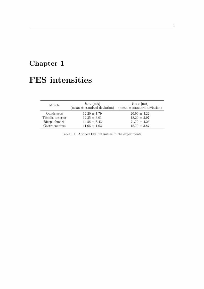
Muscle IMIN [mA] IMAX [mA](mean ± standard deviation) (mean ± standard deviation)

Quadriceps 12.20 ± 1.79 20.90 ± 4.22Tibialis anterior 12.35 ± 3.01 18.20 ± 3.97Biceps femoris 14.55 ± 3.43 21.70 ± 4.26Gastrocnemius 11.65 ± 1.63 18.70 ± 3.87

Table 1.1: Applied FES intensties in the experiments.

2

Chapter 2

Performance evaluation insimulation

We evaluated the performance of the system identification algorithm in simulation using two sys-tems G1 and G2. Based on some pre-tests, these systems were similar to the ones that wereexpected to be encountered in the experiments. G1 and G2 are first-order and second-order sys-tems, respectively, with following discrete-time representations (Ts = 0.3s):

G1 =0.2z−27

1− 0.95z−1(2.1)

G2 =0.3 + 0.01z−1 − 0.3z−2

1− 2 · 0.95z−1 + 0.952z−2z−27 (2.2)

and the continuous-time representations (zero-order hold transformation):

G1 =0.2s+ 0.6838

s+ 0.171· e−8.1s (2.3)

G2 =0.3s2 + 2.121s+ 0.1169

(s+ 0.171)2· e−8.1s (2.4)

The responses of G1 and G2 were perturbed by addition of the noise derived from H1 and H2,respectively, which were based on a second-order noise model H driven by white noise ei ∼ N (0, 1):

H1 = 1.5H (2.5)

H2 = H (2.6)

H = 0.031− 0.1z−1

1− 2.012 · 0.85z−1 + 0.852z−2(2.7)

The noise model H was chosen similar to G2, such that for G2 the perturbation was compatiblewith the ARX-structure noise model assumption. Accordingly, the perturbed output was:

ym,i = 60 + yi + ni (2.8)

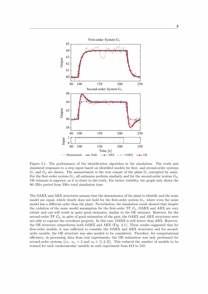
where i = 1, 2 is the index of the corresponding system G, ym,i is the measured output, yi theoutput of the TF Gi, and ni the noise from the noise model Hi. For the output offset, the reasonablevalue of 60 was considered.To evaluate the capability of the identification algorithm in determining the true underlying system,the algorithm was applied on the perturbed output (i.e., ym) of the systems, and simulated outputsfrom the estimated models and the true systems G1 and G2 were compared. A sample responseand predicted outputs of the estimated models by the estimation algorithm are presented in Fig.2.1.

3

OEOARXARXTruthMeasurement

Inpu

t

Second-order System G2

Out

put

First-order System G1

80 100 150 200 250

80 100 150 200 250

80 100 150 200 250

01

58

60

62

64

66

60

61

62

63

64

65

Out

put

Time [s]

Figure 2.1: The performance of the identification algorithm in the simulation. The truth andsimulated responses to a step input based on identified models for first- and second-order systemsG1 and G2 are shown. The measurement is the true output of the plant Gi corrupted by noise.For the first-order system G1, all estimates perform similarly and for the second-order system G2,OE estimate is superior, as it is closer to the truth. For better visibility, the graph only shows the80–250 s period from 330 s total simulation time.

The OARX and ARX structures assume that the denominator of the plant to identify and the noisemodel are equal, which clearly does not hold for the first-order system G1, where even the noisemodel has a different order than the plant. Nevertheless, the simulation result showed that despitethe violation of the noise model assumption for the first-order TF G1, OARX and ARX are veryrobust and can still result in quite good estimates, similar to the OE estimate. However, for thesecond-order TF G2, in spite of good estimation of the gain, the OARX and ARX structures werenot able to capture the overshoot properly. In this case, OARX is still better than ARX. However,the OE structure outperforms both OARX and ARX (Fig. 2.1). These results suggested that forfirst-order models, it was sufficient to consider the OARX and ARX structures and for second-order models, the OE structure was also needed to be considered. Therefore, for computationalefficiency, in processing data from real experiments, the OE estimation was only performed forsecond-order systems (i.e., na = 2 and nb ∈ [1, 2, 3]). This reduced the number of models to betrained for each cardiovascular variable in each experiment from 612 to 510.

4

Chapter 3

Proof of linear and nonlinear partdecoupling in Hammerstein modelstructure under step input

Similar as the proof in [1], consider f(u) to be an unknown nonlinear function (see Fig. 2 in themanuscript) and a step input u(k) = (0 ∨ 1). As a result, f(u) can be represented by a linearaffine function u(k) = f(u(k)) = η0 + η1u(k) ∀k with u(k) = 0∨ 1. Although η0 and η1 depend onunknown f(.), they are well-defined and can be determined uniquely:(

f(0)f(1)

)=

(η0 + η1.0η0 + η1.1

)=

(η0

η0 + η1

)

⇒(η0η1

)=

(f(0)

f(1)− f(0)

) (3.1)

with assumption that identification is feasible f(0) 6= f(1) and thus η1 6= 0. Since the TF ofa casual discrete-time system can be defined as unilateral z-transform of its unit pulse responseh = (θ0, θ1, ...) [2], G(z) =

∑∞i=0 θiz

−i. Accordingly, by normalizing the gain of f(u) to be unit(i.e., η1 = 1) the Hammerstein model can be reformulated as [1]:

y(k) = G(~θ, z)u(k) + v(k)

=∑∞

i=0θiz−i(η0 + η1u(k)) + v(k)

=∑∞

i=0θi(η0 + 1.u(k − i)) + v(k) (3.2)

= d+∑∞

i=0θiu(k − i) + v(k)

where d = η0∑∞

i=0 θi. Apparently Eq. 3.2 is an affine equation between y and u independent ofthe nonlinear function f(.), and without the constant offset term d, it turns into a linear equation.Therefore similar to PRBS, under a step input, after estimation and correction of the offset d,identification of the linear part of the Hammerstein model can be treated as a linear problem andthe unknown nonlinearity f(.) can be ignored.

5

Chapter 4

Signal-difference-to-noise ratio(SDNR)

In the context of the cardiovascular parameters, we defined SDNR as the ratio between meanchange introduced by the stimuli to the cardiovascular biosignal, and the average natural oscillationobserved in the biosignal:

SDNR =µ2 − µ1

σ1&2(4.1)

where µ1 and µ2 are respectively mean of the biosignal at zero and full stimuli computed duringcertain intervals where steady-state was expected (see Section II.D7 Input Design in the paper).σ1&2 is the average natural oscillation observed in the biosignal, and it is calculated by averagingthe standard deviation of the biosignal during the two intervals. For study protocol 1 (inclination),the first interval was chosen as the last 90 s before tilt-up and the second interval as the last 90 sbefore tilt-down. For study protocols 2 and 3 (stepping protocols), SDNR was calculated based onthe biosignal values during the last 2 min before stepping and the last 2 min of the stepping. TheSDNR was calculated once for the identification (training and validation) set (SDNR(ID)) andonce for the testing set (SDNR(test)). Similarly for study protocol 4 (FES amplitude change),SDNR was calculated for two occasions, first for the step-up phase using the last 2 min beforemaximum FES amplitude and the last 2 min of maximum amplitude (SDNR (up)), and second forthe step-down phase using the last 2 min of maximum FES amplitude and the last 2 min of thestudy protocol (SDNR (down)). The results are detailed in corresponding tables of Chapter 5.The average absolute SDNR values over all the outputs on the identification set SDNR (ID) were(Mean±SD): 5.21±4.03, 1.15±0.82, 1.32±1.20, and 0.97±0.79 for inclination, stepping withoutFES, stepping with FES, and FES amplitude inputs, respectively. This suggests that for theinputs except the inclination input, the steady-state change is as big as the natural oscillationsand in the case of FES amplitude even smaller.

6

Chapter 5

Identified transfer functions

This chapter provides information regarding the identified models for each subject in response toeach applied external stimuli.

7

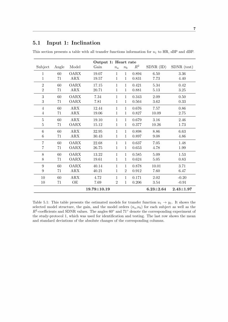
5.1 Input 1: Inclination

This section presents a table with all transfer functions information for u1 to HR, sBP and dBP.

Output 1: Heart rateSubject Angle Model Gain na nb R2 SDNR (ID) SDNR (test)

1 60 OARX 19.07 1 1 0.894 6.50 3.361 71 ARX 19.57 1 1 0.831 7.73 4.40

2 60 OARX 17.15 1 1 0.421 5.34 0.422 71 ARX 20.71 1 1 0.881 5.13 3.25

3 60 OARX 7.34 1 1 0.343 2.09 0.503 71 OARX 7.81 1 1 0.564 3.62 0.33

4 60 ARX 12.44 1 1 0.676 7.57 0.864 71 ARX 19.06 1 1 0.827 10.09 2.75

5 60 ARX 19.10 1 1 0.679 3.16 2.465 71 OARX 15.12 1 1 0.377 10.26 1.73

6 60 ARX 32.95 1 1 0.898 8.86 6.636 71 ARX 30.43 1 1 0.897 9.08 4.86

7 60 OARX 22.68 1 1 0.637 7.05 1.487 71 OARX 26.75 1 1 0.653 4.78 1.99

8 60 OARX 13.22 1 1 0.585 5.09 1.538 71 OARX 19.61 1 1 0.624 5.05 0.83

9 60 OARX 40.14 1 1 0.878 10.01 3.719 71 ARX 40.21 1 2 0.912 7.60 6.47

10 60 ARX 4.72 1 1 0.171 2.02 -0.2010 71 OE 7.69 2 1 0.206 3.54 -0.91

19.79±10.19 6.23±2.64 2.43±1.97

Table 5.1: This table presents the estimated models for transfer function u1 → y1. It shows theselected model structure, the gain, and the model orders (na,nb) for each subject as well as theR2-coefficients and SDNR values. The angles 60◦ and 71◦ denote the corresponding experiment ofthe study-protocol 1, which was used for identification and testing. The last row shows the meanand standard deviations of the absolute changes of the corresponding columns.

8

Output 2: Systolic blood pressureSubject Angle Model Gain na nb R2 SDNR (ID) SDNR (test)

1 60 OE -5.50 2 1 -0.758 -0.74 -1.631 71 ARX -3.76 1 1 0.646 -4.16 -2.98

2 60 ARX 3.51 1 2 -0.179 2.08 2.352 71 ARX 12.94 1 1 -0.718 3.59 2.05

3 60 ARX -5.81 1 1 0.261 -1.37 -0.193 71 Mean 0.00 0 0 0.020 -1.20 -1.77

4 60 OARX 18.87 1 2 0.588 10.92 5.544 71 OARX 16.29 1 1 0.842 12.63 5.21

5 60 ARX -5.10 1 1 0.237 -1.70 -0.295 71 Mean 0.00 0 0 0.003 -0.09 1.02

6 60 Mean 0.00 0 0 -0.020 -0.61 0.116 71 Mean 0.00 0 0 0.007 0.12 -0.28

7 60 OARX 17.71 1 1 0.753 5.01 1.937 71 ARX 14.49 1 1 0.383 2.64 1.55

8 60 OARX -9.42 1 2 -0.323 -2.27 -1.438 71 OE -1.71 2 1 0.204 -1.95 -0.08

9 60 OARX -11.49 1 1 -0.018 -1.97 -3.149 71 ARX -23.90 1 2 0.716 -2.63 -2.08

10 60 ARX 10.04 1 1 0.707 1.96 2.4110 71 ARX 20.96 1 1 0.872 7.21 5.82

9.07±7.67 3.24±3.39 2.09±1.75

Table 5.2: This table presents the estimated models for the transfer function u1 → y2 in the samestructure as table 5.1.

9

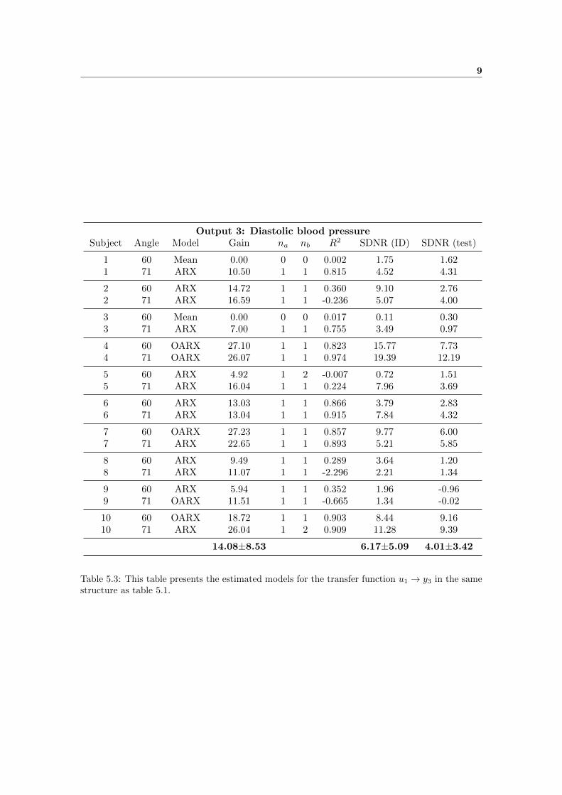
Output 3: Diastolic blood pressureSubject Angle Model Gain na nb R2 SDNR (ID) SDNR (test)

1 60 Mean 0.00 0 0 0.002 1.75 1.621 71 ARX 10.50 1 1 0.815 4.52 4.31

2 60 ARX 14.72 1 1 0.360 9.10 2.762 71 ARX 16.59 1 1 -0.236 5.07 4.00

3 60 Mean 0.00 0 0 0.017 0.11 0.303 71 ARX 7.00 1 1 0.755 3.49 0.97

4 60 OARX 27.10 1 1 0.823 15.77 7.734 71 OARX 26.07 1 1 0.974 19.39 12.19

5 60 ARX 4.92 1 2 -0.007 0.72 1.515 71 ARX 16.04 1 1 0.224 7.96 3.69

6 60 ARX 13.03 1 1 0.866 3.79 2.836 71 ARX 13.04 1 1 0.915 7.84 4.32

7 60 OARX 27.23 1 1 0.857 9.77 6.007 71 ARX 22.65 1 1 0.893 5.21 5.85

8 60 ARX 9.49 1 1 0.289 3.64 1.208 71 ARX 11.07 1 1 -2.296 2.21 1.34

9 60 ARX 5.94 1 1 0.352 1.96 -0.969 71 OARX 11.51 1 1 -0.665 1.34 -0.02

10 60 OARX 18.72 1 1 0.903 8.44 9.1610 71 ARX 26.04 1 2 0.909 11.28 9.39

14.08±8.53 6.17±5.09 4.01±3.42

Table 5.3: This table presents the estimated models for the transfer function u1 → y3 in the samestructure as table 5.1.

10

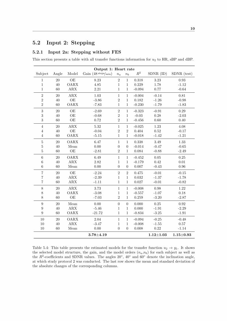
5.2 Input 2: Stepping

5.2.1 Input 2a: Stepping without FES

This section presents a table with all transfer functions information for u2 to HR, sBP and dBP.

Output 1: Heart rateSubject Angle Model Gain (48 steps/min) na nb R2 SDNR (ID) SDNR (test)

1 20 OE 8.23 2 1 0.318 3.23 0.931 40 OARX 4.85 1 1 0.229 1.78 -1.121 60 ARX 2.21 1 1 -0.094 0.77 -0.64

2 20 ARX 1.03 1 1 -0.004 -0.14 0.812 40 OE -3.86 2 1 0.182 -1.26 -0.982 60 OARX -7.83 1 1 -0.230 -1.79 -1.83

3 20 OE -2.69 2 1 -0.323 -0.91 0.293 40 OE -0.68 2 1 -0.03 0.28 -2.033 60 OE 0.72 2 1 -0.456 0.60 0.40

4 20 ARX 5.32 1 1 -0.025 1.23 4.084 40 OE -0.04 2 2 0.404 0.52 -0.174 60 OARX -5.15 1 1 -0.018 -1.42 -1.21

5 20 OARX 6.47 1 1 0.338 3.49 1.335 40 Mean 0.00 0 0 -0.014 -0.47 -0.655 60 OE -2.81 2 1 0.084 -0.88 -2.49

6 20 OARX 6.49 1 1 -0.452 0.05 0.256 40 ARX 2.82 1 1 -0.179 0.42 0.016 60 Mean 0.00 0 0 0.007 -0.43 0.96

7 20 OE -2.24 2 2 0.475 -0.01 -0.157 40 ARX -2.39 1 1 0.032 -1.37 -1.787 60 ARX -1.11 1 1 0.027 -0.01 -0.82

8 20 ARX 3.73 1 1 -0.008 0.98 1.228 40 OARX -3.08 1 1 -0.557 -1.07 0.188 60 OE -7.03 2 1 0.259 -3.20 -2.87

9 20 Mean 0.00 0 0 0.000 0.25 0.929 40 ARX -5.46 1 1 0.000 -1.91 -2.299 60 OARX -21.72 1 1 -0.834 -3.25 -1.91

10 20 OARX 2.04 1 1 -0.094 -0.25 -0.4810 40 ARX -3.47 1 1 -0.008 -1.55 0.5710 60 Mean 0.00 0 0 0.008 0.22 -1.14

3.78±4.19 1.12±1.03 1.15±0.93

Table 5.4: This table presents the estimated models for the transfer function u2 → y1. It showsthe selected model structure, the gain, and the model orders (na,nb) for each subject as well asthe R2-coefficients and SDNR values. The angles 20◦, 40◦ and 60◦ denote the inclination angle,at which study protocol 2 was conducted. The last row shows the mean and standard deviation ofthe absolute changes of the corresponding columns.

11

Output 2: Systolic blood pressureSubject Angle Model Gain (48 steps/min) na nb R2 SDNR (ID) SDNR (test)

1 20 Mean 0.00 0 0 0.004 -0.42 -0.131 40 ARX 6.04 1 1 0.116 1.02 2.471 60 OE 8.37 2 1 0.244 2.48 1.21

2 20 Mean 0.00 0 0 0.002 -1.67 2.162 40 Mean 0.00 0 0 0.013 0.00 -0.192 60 OARX 3.23 1 1 0.039 0.52 -0.49

3 20 ARX -3.44 1 1 -0.210 -1.10 0.783 40 OE 2.37 2 1 0.102 0.72 -1.483 60 ARX 4.32 1 1 0.182 2.11 -1.03

4 20 Mean 0.00 0 0 0.009 -0.96 -0.814 40 Mean 0.00 0 0 0.016 0.34 2.364 60 Mean 0.00 0 0 -0.005 0.92 0.94

5 20 ARX 1.31 1 1 0.194 0.86 1.555 40 ARX 5.33 1 1 0.495 1.64 3.315 60 ARX 12.41 1 1 -0.935 3.57 1.88

6 20 OARX -4.79 1 1 -0.150 -1.50 0.076 40 OARX -2.00 1 1 -0.014 -0.96 0.256 60 ARX 3.11 1 1 -0.168 1.54 1.24

7 20 Mean 0.00 0 0 -0.001 -0.13 -1.387 40 ARX 3.76 1 1 0.062 1.64 1.407 60 ARX 5.29 1 1 0.359 1.71 1.37

8 20 ARX -1.98 1 1 -0.027 -0.83 -0.948 40 Mean 0.00 0 0 0.000 -0.81 0.788 60 ARX -0.61 1 1 -0.027 0.38 1.34

9 20 ARX -0.25 1 1 0.000 -0.39 -1.419 40 ARX 6.54 1 1 0.536 1.57 1.999 60 OARX 7.60 1 1 0.208 0.90 0.87

10 20 ARX 1.30 1 1 0.066 1.76 -0.0510 40 Mean 0.00 0 0 -0.003 -1.35 -3.2610 60 ARX 4.08 1 1 0.165 1.87 5.10

2.94±3.11 1.19±0.76 1.41±1.10

Table 5.5: This table presents the estimated models for the transfer function u2 → y2 in the samestructure as table 5.4.

12

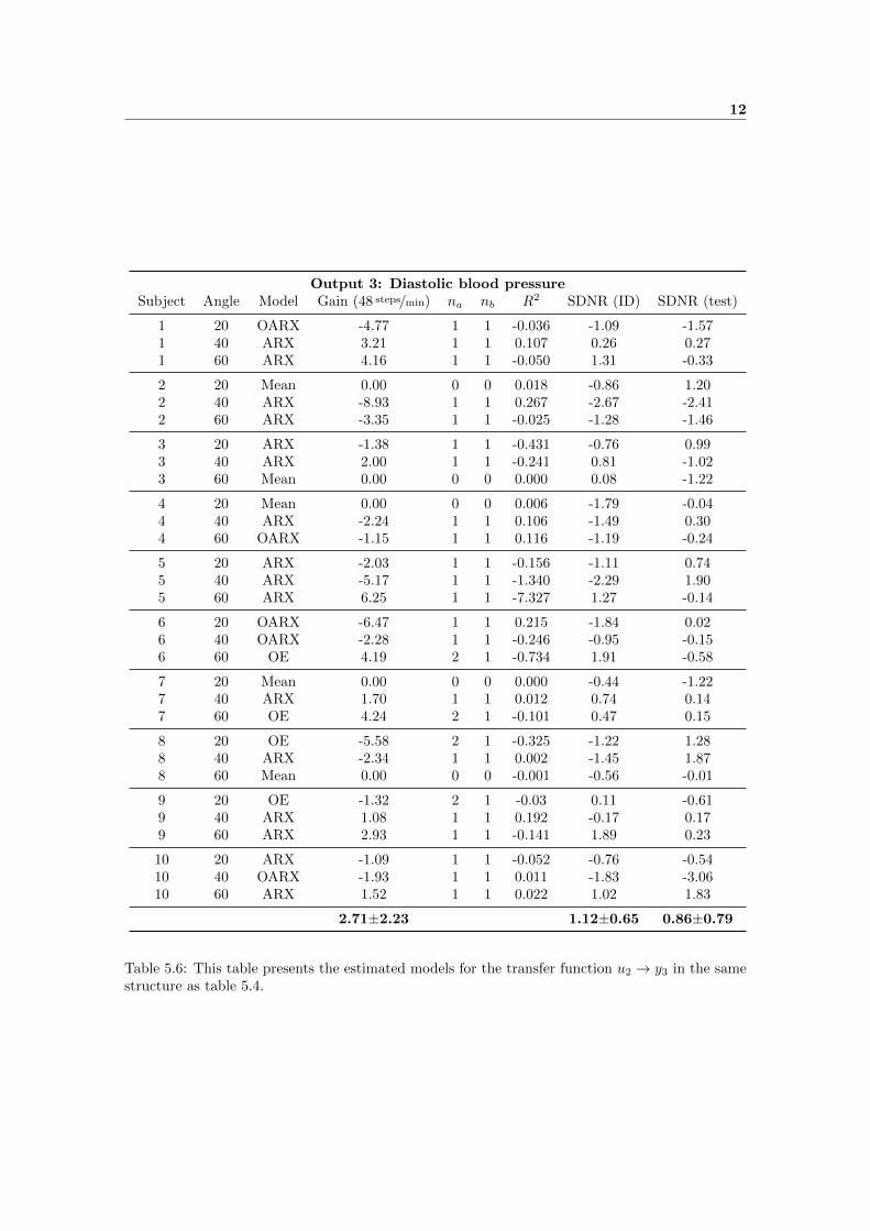
Output 3: Diastolic blood pressureSubject Angle Model Gain (48 steps/min) na nb R2 SDNR (ID) SDNR (test)

1 20 OARX -4.77 1 1 -0.036 -1.09 -1.571 40 ARX 3.21 1 1 0.107 0.26 0.271 60 ARX 4.16 1 1 -0.050 1.31 -0.33

2 20 Mean 0.00 0 0 0.018 -0.86 1.202 40 ARX -8.93 1 1 0.267 -2.67 -2.412 60 ARX -3.35 1 1 -0.025 -1.28 -1.46

3 20 ARX -1.38 1 1 -0.431 -0.76 0.993 40 ARX 2.00 1 1 -0.241 0.81 -1.023 60 Mean 0.00 0 0 0.000 0.08 -1.22

4 20 Mean 0.00 0 0 0.006 -1.79 -0.044 40 ARX -2.24 1 1 0.106 -1.49 0.304 60 OARX -1.15 1 1 0.116 -1.19 -0.24

5 20 ARX -2.03 1 1 -0.156 -1.11 0.745 40 ARX -5.17 1 1 -1.340 -2.29 1.905 60 ARX 6.25 1 1 -7.327 1.27 -0.14

6 20 OARX -6.47 1 1 0.215 -1.84 0.026 40 OARX -2.28 1 1 -0.246 -0.95 -0.156 60 OE 4.19 2 1 -0.734 1.91 -0.58

7 20 Mean 0.00 0 0 0.000 -0.44 -1.227 40 ARX 1.70 1 1 0.012 0.74 0.147 60 OE 4.24 2 1 -0.101 0.47 0.15

8 20 OE -5.58 2 1 -0.325 -1.22 1.288 40 ARX -2.34 1 1 0.002 -1.45 1.878 60 Mean 0.00 0 0 -0.001 -0.56 -0.01

9 20 OE -1.32 2 1 -0.03 0.11 -0.619 40 ARX 1.08 1 1 0.192 -0.17 0.179 60 ARX 2.93 1 1 -0.141 1.89 0.23

10 20 ARX -1.09 1 1 -0.052 -0.76 -0.5410 40 OARX -1.93 1 1 0.011 -1.83 -3.0610 60 ARX 1.52 1 1 0.022 1.02 1.83

2.71±2.23 1.12±0.65 0.86±0.79

Table 5.6: This table presents the estimated models for the transfer function u2 → y3 in the samestructure as table 5.4.

13

5.2.2 Input 2b: Stepping with minimum FES

This section presents a table with all transfer functions information for u2 to HR, sBP and dBP.

Output 1: Heart rateSubject Angle Model Gain (48 steps/min) na nb R2 SDNR (ID) SDNR (test)

1 20 ARX 2.37 1 1 -0.167 0.55 1.111 40 OARX -2.38 1 1 0.100 -0.34 -1.081 60 OARX 2.35 1 1 -0.435 -0.13 -0.16

2 20 ARX 2.06 1 1 0.071 0.91 0.582 40 Mean 0.00 0 0 0.002 -1.49 -1.002 60 ARX -7.50 1 1 0.500 -3.32 -1.21

3 20 OE -0.51 2 1 -0.048 -0.33 -0.413 40 OARX -2.23 1 1 -0.043 -1.40 -0.223 60 OARX -2.59 1 1 0.189 -0.28 -0.98

4 20 ARX 2.81 1 1 0.033 0.24 0.614 40 ARX 1.82 1 1 0.101 -0.04 0.884 60 OARX 4.52 1 1 0.489 1.41 0.52

5 20 OE -0.15 2 2 0.632 0.69 1.495 40 Mean 0.00 0 0 0.002 -0.47 0.565 60 ARX -5.36 1 1 0.434 -1.95 -1.23

6 20 ARX -1.03 1 1 -0.028 -0.40 -2.746 40 OARX -5.32 1 1 0.065 -0.95 -2.906 60 ARX 1.30 1 1 -0.098 0.77 -0.60

7 20 OE -4.84 2 1 0.059 -1.01 0.417 40 OE -2.65 2 1 -0.131 0.04 0.247 60 Mean 0.00 0 0 0.001 -0.02 0.21

8 20 ARX 0.93 1 1 -0.011 -0.03 -0.028 40 OARX -4.70 1 1 -0.414 -1.64 -1.358 60 OARX -5.47 1 1 0.649 -2.79 -1.27

9 20 OARX 3.39 1 1 -0.342 1.78 -1.979 40 OE -9.01 2 1 0.135 -2.88 -2.339 60 OE -10.68 2 1 -0.026 -2.07 -1.05

10 20 OARX -3.36 1 1 -0.213 -1.78 -0.5810 40 OARX 0.94 1 1 -0.074 0.91 0.9210 60 OARX -2.79 1 1 0.103 -1.07 -0.47

3.10±2.64 1.06±0.91 0.97±0.73

Table 5.7: This table presents the estimated models for transfer function u2 → y1 in the samestructure as table 5.4 but for the case, where minimum FES is applied (i.e., study protocol 3).

14

Output 2: Systolic blood pressureSubject Angle Model Gain (48 steps/min) na nb R2 SDNR (ID) SDNR (test)

1 20 OE 3.31 2 1 0.220 1.58 0.711 40 ARX 3.86 1 1 0.394 0.93 1.231 60 ARX 5.72 1 1 0.092 3.05 -0.08

2 20 ARX 2.09 1 1 0.036 -0.34 -0.072 40 Mean 0.00 0 0 -0.007 0.25 -0.082 60 OARX 2.97 1 1 -0.125 1.09 -1.01

3 20 Mean 0.00 0 0 0.010 -0.28 0.203 40 Mean 0.00 0 0 0.006 0.87 -1.003 60 ARX -1.62 1 1 -0.074 -0.39 1.22

4 20 Mean 0.00 0 0 0.003 -0.88 -1.124 40 OARX 4.41 1 1 -0.028 1.49 -0.014 60 OARX 4.83 1 1 0.059 1.47 0.35

5 20 OARX -8.43 1 1 -0.681 -6.48 1.755 40 ARX 5.65 1 1 0.296 1.31 1.595 60 OARX 13.60 1 1 -0.434 4.45 0.88

6 20 ARX -5.13 1 1 -0.218 -0.56 -1.116 40 Mean 0.00 0 0 -0.005 -0.79 -0.816 60 ARX 4.58 1 1 0.119 2.39 1.05

7 20 Mean 0.00 0 0 0.007 -0.51 0.847 40 ARX 7.53 1 1 0.471 0 1.49 1.287 60 Mean 0.00 0 0 -0.012 -0.61 1.09

8 20 ARX -5.73 1 1 0.012 -1.02 -0.458 40 Mean 0.00 0 0 0.004 -0.48 -1.768 60 ARX -1.27 1 1 -0.086 -0.11 0.98

9 20 ARX -2.27 1 1 -0.020 -0.98 -1.309 40 ARX -3.23 1 1 -0.480 -2.14 0.799 60 OARX 6.59 1 1 0.070 1.95 2.28

10 20 Mean 0.00 0 0 -0.007 0.79 -1.6410 40 ARX -1.90 1 1 -0.156 -0.10 1.0610 60 ARX 5.66 1 1 -0.019 5.03 -3.19

3.35±3.23 1.46±1.51 1.03±0.69

Table 5.8: This table presents the estimated models for the transfer function u2 → y2 in the samestructure as table 5.4 but for the case, where FES is on.

15

Output 3: Diastolic blood pressureSubject Angle Model Gain (48 steps/min) na nb R2 SDNR (ID) SDNR (test)

1 20 OE 2.72 2 1 0.041 1.64 0.541 40 ARX 2.08 1 1 0.214 0.51 0.721 60 OE 6.48 2 1 -0.303 2.07 -0.61

2 20 Mean 0.00 0 0 0.008 -0.91 0.472 40 ARX -3.12 1 1 -0.289 -2.32 0.232 60 OARX -3.01 1 1 0.382 -2.60 -2.27

3 20 ARX -0.56 1 1 -0.044 0.10 -0.133 40 ARX -0.77 1 1 0.002 -1.11 -0.693 60 ARX -2.27 1 1 -0.096 -1.01 0.33

4 20 ARX -4.25 1 1 -0.177 -2.64 -0.664 40 OE 2.87 2 1 0.021 -0.10 0.414 60 OE -0.96 2 1 -0.018 -0.36 0.82

5 20 ARX -6.53 1 1 -0.352 -4.47 1.035 40 Mean 0.00 0 0 -0.001 0.52 0.525 60 OARX 6.66 1 1 -0.461 3.28 -0.67

6 20 ARX -7.31 1 1 -0.446 -2.46 -1.626 40 ARX -2.34 1 1 -0.054 -1.88 -1.076 60 Mean 0.00 0 0 0.022 0.87 0.15

7 20 ARX -3.36 1 1 -0.060 -1.45 0.397 40 ARX -0.18 1 1 -0.020 -0.60 0.857 60 Mean 0.00 0 0 -0.012 -0.83 0.62

8 20 ARX -2.50 1 1 0.006 -1.13 -2.568 40 OARX -4.60 1 1 -0.254 -1.75 -2.318 60 ARX -3.58 1 1 -0.286 -1.80 0.34

9 20 OE -2.25 2 1 -0.085 -0.33 -1.519 40 OARX -4.30 1 1 0.138 -3.52 -0.799 60 OARX 2.25 1 1 0.237 1.44 1.39

10 20 OARX -2.31 1 1 0.559 -0.08 -1.9610 40 ARX -0.18 1 1 -0.023 -0.38 0.2410 60 OARX 1.47 1 1 0.015 0.98 -2.35

2.63±2.13 1.44±1.10 0.94±0.72

Table 5.9: This table presents the estimated models for the transfer function u2 → y3 in the samestructure as table 5.4 but for the case, where FES is on.

16

5.3 Input 3: FES amplitude

This section presents a table with all transfer functions information for u3 to HR, sBP and dBP.

17

Output 1: Heart rateSubject Angle Model Gain na nb R2 SDNR (up) SDNR (down)

1 0 Mean 0.00 0 0 -0.004 0.37 -1.411 20 OARX 3.18 1 1 0.292 1.79 -1.201 40 ARX 2.26 1 1 -0.418 0.89 0.011 60 ARX 3.44 1 1 0.152 0.13 -1.12

2 0 Mean 0.00 0 0 -0.004 -1.26 0.372 20 ARX 2.65 1 1 -0.420 1.15 0.152 40 ARX 6.70 1 1 -1.250 0.46 1.032 60 ARX 2.18 1 1 0.211 0.41 -0.76

3 0 Mean 0.00 0 0 -0.025 0.02 -0.743 20 ARX 0.75 1 1 0.468 0.51 -0.663 40 ARX -1.13 1 1 -0.704 -0.94 -0.493 60 OARX 2.51 1 1 -0.262 0.63 -0.09

4 0 Mean 0.00 0 0 -0.002 2.40 0.164 20 OARX -4.51 1 1 -0.461 -1.41 -2.364 40 ARX -1.81 1 1 -0.552 -0.86 0.724 60 ARX 2.91 1 1 -1.915 1.83 -0.67

5 0 Mean 0.00 0 0 -0.041 -0.29 1.875 20 OARX -7.06 1 1 -7.294 -4.03 1.515 40 Mean 0.00 0 0 0.002 0.31 0.855 60 Mean 0.00 0 0 0.037 0.87 0.51

6 0 Mean 0.00 0 0 0.028 0.11 -0.866 20 ARX -1.95 1 1 -0.636 -1.35 -0.156 40 OARX -15.11 1 1 -0.617 -3.26 0.116 60 ARX -20.14 1 1 0.590 -2.39 4.88

7 0 OARX 1.64 1 1 0.677 0.42 -1.397 20 OARX 3.12 1 1 0.786 1.07 -1.327 40 ARX 4.40 1 1 0.021 0.79 -1.027 60 ARX -1.77 1 1 -0.142 -0.59 -0.23

8 0 ARX -2.22 1 1 -0.921 -1.17 1.878 20 Mean 0.00 0 0 0.007 -0.06 0.408 40 ARX 1.78 1 1 0.595 0.94 -1.538 60 ARX 1.14 1 1 -0.778 1.01 -0.69

9 0 ARX 0.54 1 1 0.373 0.69 -0.179 20 ARX 4.43 1 1 0.763 1.63 -1.469 40 OARX 3.52 1 1 -0.208 0.71 -0.589 60 ARX 1.65 1 1 0.400 0.57 -1.33

10 0 OARX 1.60 1 1 0.448 0.16 0.4610 20 Mean 0.00 0 0 -0.005 0.27 -0.0110 40 ARX -1.89 1 1 0.084 0.06 -0.0110 60 OARX -2.91 1 1 -0.232 -1.46 0.63

2.77±3.92 0.98±0.87 0.89±0.87

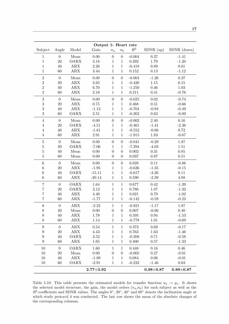
Table 5.10: This table presents the estimated models for transfer function u3 → y1. It showsthe selected model structure, the gain, the model orders (na,nb) for each subject as well as theR2-coefficients and SDNR values. The angles 0◦, 20◦, 40◦ and 60◦ denote the inclination angle atwhich study protocol 4 was conducted. The last row shows the mean of the absolute changes ofthe corresponding columns.

18

Output 2: Systolic blood pressureSubject Angle Model Gain na nb R2 SDNR (up) SDNR (down)

1 0 ARX 6.83 1 1 -1.539 1.82 -0.971 20 Mean 0.00 0 0 -0.010 1.00 -0.281 40 OARX 3.13 1 1 -2.492 0.75 -0.031 60 Mean 0.00 0 0 -0.005 -0.36 -1.84

2 0 ARX 1.53 1 1 -0.518 0.26 0.902 20 OARX 3.21 1 1 0.663 1.80 -1.952 40 ARX 0.91 1 1 0.248 0.83 -0.642 60 Mean 0.00 0 0 -0.001 -0.26 -0.19

3 0 Mean 0.00 0 0 0.058 0.35 -0.493 20 ARX 2.53 1 1 0.619 0.79 -0.723 40 OARX -3.29 1 1 -5.766 -2.06 0.853 60 ARX -0.80 1 1 -0.484 -1.09 -0.94

4 0 Mean 0.00 0 0 0.008 1.26 0.084 20 ARX -6.01 1 1 0.614 -2.60 2.254 40 ARX -4.33 1 1 -1.509 -1.42 -2.524 60 ARX -5.06 1 1 -0.364 -0.88 2.54

5 0 OARX -2.65 1 1 0.329 0.12 0.005 20 ARX -2.19 1 1 0.336 -1.69 5.015 40 ARX -0.05 1 1 -0.031 -2.28 1.585 60 ARX 3.81 1 1 -0.578 1.17 1.83

6 0 ARX -1.88 1 1 -1.769 -0.14 -0.826 20 ARX -1.12 1 1 -0.507 -0.72 -0.216 40 Mean 0.00 0 0 -0.076 0.49 0.106 60 Mean 0.00 0 0 0.000 -0.28 0.97

7 0 ARX 4.65 1 1 -0.629 1.31 -1.337 20 Mean 0.00 0 0 0.001 -0.75 -1.067 40 ARX 2.47 1 1 -0.791 0.54 -0.357 60 Mean 0.00 0 0 -0.001 0.50 -0.59

8 0 Mean 0.00 0 0 -0.015 1.26 1.578 20 Mean 0.00 0 0 -0.007 0.70 0.528 40 Mean 0.00 0 0 -0.005 -1.28 -1.938 60 Mean 0.00 0 0 -0.008 0.35 -1.06

9 0 Mean 0.00 0 0 -0.011 -0.89 -2.669 20 Mean 0.00 0 0 -0.006 0.11 0.359 40 ARX -0.39 1 1 -0.133 -0.77 -1.339 60 ARX 3.93 1 1 0.751 1.63 -1.86

10 0 Mean 0.00 0 0 0.000 -0.21 -0.1710 20 ARX -5.78 1 1 -1.905 -3.32 1.1310 40 ARX -2.86 1 1 -0.435 -1.26 -2.4710 60 Mean 0.00 0 0 -0.012 .78 -5.18

1.73±2.05 1.03±0.73 1.28±1.18

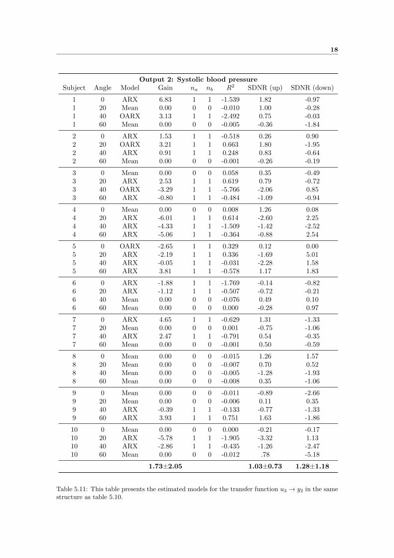
Table 5.11: This table presents the estimated models for the transfer function u3 → y2 in the samestructure as table 5.10.

19

Output 3: Diastolic blood pressureSubject Angle Model Gain na nb R2 SDNR (up) SDNR (down)

1 0 ARX 4.13 1 1 0.046 1.68 -1.071 20 Mean 0.00 0 0 -0.012 0.67 0.111 40 Mean 0.00 0 0 0.000 -0.10 -0.251 60 Mean 0.00 0 0 0.003 -0.78 -1.31

2 0 OARX 3.97 1 1 -0.288 0.18 0.562 20 Mean 0.00 0 0 -0.013 1.52 -2.342 40 Mean 0.00 0 0 0.002 0.40 0.002 60 Mean 0.00 0 0 -0.006 -0.11 -0.51

3 0 ARX -0.76 1 1 0.447 0.03 0.573 20 ARX -0.22 1 1 -0.143 -1.13 0.273 40 OARX -0.86 1 1 -1.521 -0.84 0.043 60 ARX 1.04 1 1 0.378 0.20 -1.84

4 0 Mean 0.00 0 0 0.022 0.71 0.984 20 ARX -1.31 1 1 0.349 -1.70 1.294 40 ARX -1.77 1 1 -0.661 -0.76 -3.604 60 ARX -1.66 1 1 -0.126 -2.22 3.32

5 0 OARX -1.93 1 1 -1.295 -0.14 -0.895 20 ARX -2.18 1 1 0.491 -2.15 2.445 40 Mean 0.00 0 0 -0.009 -1.93 0.355 60 Mean 0.00 0 0 0.003 1.15 2.23

6 0 ARX -1.06 1 1 -0.705 -0.01 -0.646 20 ARX -0.96 1 1 -0.399 -0.94 -0.096 40 Mean 0.00 0 0 -0.023 -0.30 0.426 60 ARX -1.09 1 1 0.419 -0.45 0.67

7 0 ARX 1.30 1 1 0.786 1.01 -1.677 20 ARX -3.67 1 1 -0.497 -1.14 -1.577 40 Mean 0.00 0 0 -0.028 0.27 -0.237 60 Mean 0.00 0 0 -0.002 0.26 -0.55

8 0 ARX 3.95 1 1 -0.936 1.73 0.368 20 ARX -1.31 1 1 0.338 -0.25 0.258 40 Mean 0.00 0 0 -0.001 -1.51 -0.218 60 Mean 0.00 0 0 0.002 -0.23 -0.14

9 0 Mean 0.00 0 0 -0.003 -1.23 -4.849 20 ARX 2.38 1 1 0.173 0.92 -0.579 40 OARX -2.58 1 1 -1.169 -1.96 0.989 60 ARX 3.35 1 1 0.732 0.90 -1.93

10 0 Mean 0.00 0 0 0.004 -0.44 0.2710 20 ARX -2.80 1 1 -3.073 -3.42 1.3510 40 OARX -0.26 1 1 -0.035 -0.09 -2.0310 60 Mean 0.00 0 0 0.017 0.87 -5.27

1.11±1.33 0.91±0.76 1.20±1.27

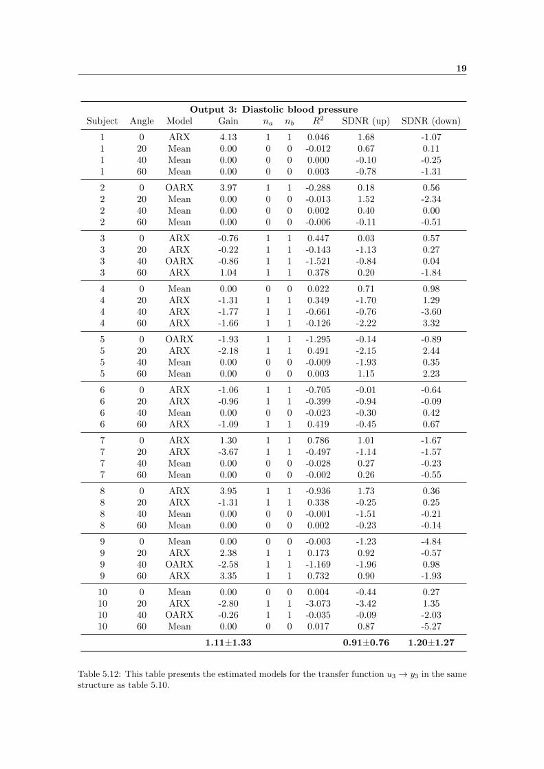
Table 5.12: This table presents the estimated models for the transfer function u3 → y3 in the samestructure as table 5.10.

20

Bibliography

[1] Er-Wei Bai. Decoupling the linear and nonlinear parts in hammerstein model identification.Automatica, 40(4):671–676, 2004.

[2] William S Levine. The control handbook. CRC press, 1996.