Modeling the 20 November 2003 Ionosphere Storm withGRACE

Seebany Datta-Barua, Todd Walter, Sam Pullen, and Per EngeStanford University

ABSTRACT

The Local Area Augmentation System (LAAS) providesdifferential GPS corrections for Category I precisionapproach to aviation users within tens of kilometers ofthe LAAS Ground Facility (LGF). To ensure integrity,any circumstance that may lead to hazardously misleadinginformation (HMI) being transmitted to the user must beidentified. If the probability of the situation exceeds theallocated integrity risk, its maximum user errors must bebounded by one or more user-computed protection levels.Over short baselines, the differential ionosphere errorbetween a user and LGF can pose one such threat.

This work examines how the spatial rate of change ofthe ionosphere over baselines of tens of kilometers canbe modeled to provide insight into hazardous conditions.We develop a static spatial model of the ionosphere basedon a technique developed for understanding the impacton WAAS of the 31 October 2003 localized nighttimeionosphere enhancement. In this work we apply themethod to the 20 November 2003 ionosphere storm, a dayon which GPS observations of the disturbed ionospherewere previously used to populate the space of possibleionosphere threats to LAAS users.

This 3-D model assigns vertical profiles to latitude andlongitude regions. The horizontal “enhancement” and“background” ionosphere regions are identified basedon measurements made by the Continuously OperatingReference Stations (CORS). Since observations of verticaldensity variations are limited with GPS receivers on theground, space-based GPS data from on board one of theGRACE satellites passing through the disturbed iono-sphere around 19:40 UT is used to test a range of verticalelectron density profiles. The 500 km orbital altitude ofthe GRACE satellites effectively limits the contribution tothe total electron content of the topside and plasmasphere.After finding the electron density model that minimizes

the mean squared error, we then integrate through thelines of sight of a set of CORS receivers located in Ohioand separated by baselines as short as 50-75 km. Pairs ofthese stations mimic user-LGF pairs and were used in theliterature to estimate the possible spatial decorrelation overLAAS baselines. We integrate through the CORS lines ofsight (LOS) to compute the differential ionosphere overtens-of-kilometer baselines.

We find that a 3-D static model of the ionosphere cannotreproduce the 350-400 mm/km spatial rates of change inionosphere error that have been verified with data. How-ever, we find that allowing the ionosphere anomaly tosweep westward at 300 m/s, as has been estimated fromdata, can in fact reproduce rates of change between neigh-boring CORS stations on the order of 400 mm/km. Furtherrefinements are needed to optimize the model-predicted de-lay over the three-hour timespan of the terrestrial observa-tions, though the gross features are similar. This work con-firms that the relative velocity of the ionosphere structureand the lines of sight are an important factor in apparentgradients in the ionosphere and also helps to further val-idate the estimates made from the CORS observations ofshort baseline spatial rates of change in ionosphere delay.

INTRODUCTION

The Federal Aviation Administration’s Local AreaAugmentation System (LAAS) is a Ground-Based Aug-mentation System (GBAS) designed to provide differentialGPS corrections to users within tens of kilometers of asingle airport [6]. LAAS must meet the demands in accu-racy, availability, and integrity needed for Category II/IIIlandings. The LAAS architecture consists of the LAASGround Facility (LGF), which is a reference locationequipped with four dual-frequency GPS receivers typicallyplaced near the runway. As a DGPS system it broadcastsionosphere corrections and bounds to the user via a VHFdata broadcast (VDB).

Bounds must be placed on the difference in ionosphericerrors between an incoming aircraft and the LGF withminimal loss in availability. The ionosphere delay at areceiver is proportional to the total electron content (TEC),the integral of the electron density along the signal raypath.Because the ionosphere typically varies smoothly for auser and LGF separated by only a few kilometers, thenominal ionospheric error correction broadcast is 2-5 mmof delay difference per km of user-LGF separation distance[11]. However, to ensure user safety, what matters is notthe typical so much as the near-worst-case ionosphereconditions. Such circumstances occurred on 20 November2003.

During this event a coronal mass ejection from the sunarrived at the earth and caused extremely stormy behaviorin the ionosphere. In the North American sector a largestorm-enhanced density (SED) with equivalent verticaldelays greater than 20 m developed over the southernConterminous U.S. (CONUS) in the daytime. A long,narrow filament of enhanced electron density stretchingfrom the SED northwest toward the magnetic pole wasalso observed. Foster et al. suggested this large “tongue ofionization” (TOI) was created by electric fields effectivelychanneling electrons poleward and that it was connectedwith plasmasphere erosion [7]. This TOI region is ofinterest for the LAAS ionosphere threat model becauseobservations of some of the highest recorded spatial ratesof change over short baselines were made during itspassage over the midwestern US [4].

Extensive work has been done by Luo et al. in developingand parameterizing a threat model to represent it [12] and[13]. The anomalous ionosphere was modeled by a linearspatial rate of change of ionosphere error, a horizontaldistance over which the spatial rate of change occurs, aground speed of the anomaly, and the elevation at whichthe anomalous ionosphere is viewed. Ene et al. used datato characterize and validate events that have been observedto occur within this parameter space [5]. Lee et al. ransimulations to quantify the impact of the boundaries of thisparameter space on LAAS Cat I availability [10]. Morerecently, Park et al. have run a LAAS-like differential GPScorrections between a pseudo-user/LGF pair of stationsto confirm that the vertical position error could in factbe many meters beyond the vertical protection level, andtherefore that the conservatism built into the threat modelis justified [15].

The goal of this paper is to use ground station GPS dataover CONUS and space-borne GPS data to develop a spa-tial model of the electron density that is consistent with thespatial decorrelation rates of 400 mm/km verified in the lit-erature. We use the ground-based CORS GPS network and

the GRACE satellites with their onboard GPS receivers.The terrestrial data are used to develop a density field that ispiecewise continuous horizontally between the SED, TOI,and background regions. In each region of the model, weassign a possible vertical electron density profile. We inte-grate through the space-based GRACE GPS receiver linesof sight to find the choice of density profiles that minimizesthe mean squared error. With this three-dimensional model,we then integrate through the lines of sight in a region ofCORS with a high density of stations to predict possiblespatial gradients. In the last section we will show that a3-D electron density model cannot produce the gradientson the order of 400 mm/km that have been observed. Onthe other hand, we provide evidence that, by allowing for atime variation of the ionosphere by sweeping the TOI west-ward at 300 m/s, a simple 4-D extension of the model canin fact predict gradients of hundreds of mm of differentialdelay per km of receiver separation distance.

DATA

The Continuously Operating Reference Stations (CORS)are a network of almost 400 GPS receivers in the U.S.whose data are made publicly available in the ReceiverINdependent EXchange (RINEX) format by the NationalGeodetic Survey [16]. The CORS sites considered inparticular in this work are dual-frequency GPS receiversoperated by the Ohio Department of Transportation [14].The observations from these stations made during the 20November 2003 storm have been assimilated and leveledby the use of the Global Ionospheric Mapping (GIM)software at NASA’s Jet Propulsion Laboratory (JPL). Withthe additional use of the publicly available InternationalGNSS Service station data worldwide, GIM estimatesand removes satellite and receiver interfrequency biasesto provide high precision ionosphere measurements. Theprocessing is described in detail by Komjathy et al. [9].The data are provided at 5-minute intervals.

The Gravity Recovery and Climate Experiment (GRACE)is a NASA and DLR (Germany) science mission satellitesystem established to measure variations in earth’s gravityfield [1]. The system consists of two satellites in a near-polar orbit at 500 km altitude in the same orbital plane220 km apart. Dual-frequency Blackjack GPS receiversdeveloped at JPL are used for precise orbit determinationand atmospheric occultation on each [18]. The GPS datafrom each of the two satellites is made publicly availablefor download in RINEX format.

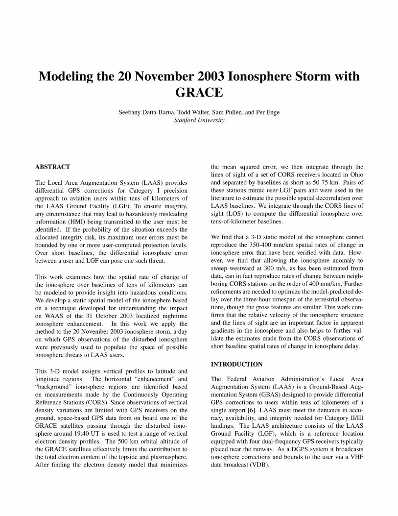
A map of the equivalent vertical delay assuming a 350km ionosphere shell height over the eastern U.S. basedon dual frequency CORS measurements on 20 November2003 at 19:38 UT are plotted in Figure 1. The color ateach point on the map corresponds to the ionosphere delay

at GPS L1 frequency, in meters from 0 (blue) to 20 (red).Figure 1a shows the ground track of the GRACE leadsatellite “A” from 19:33–19:43 UT in black as it travelsfrom south to north, and Figure 1b shows the same forGRACE-B. The satellites’ positions at 19:36:30, 19:38:00,and 19:39:00 UT are marked with a square, triangle, andcircle, respectively. From 19:33-19:43 UT GRACE-A and-B tracked several GPS satellites. Shadowed broken linesegments point from the position of each GRACE satelliteat 19:38 UT toward the GPS satellites identified by theirPRN numbers: 1, 2, 3, 7, 8, 11, 13, 27, 28, and 31. Shorterline segments point toward higher elevation satellites.

The map of delays over the eastern U.S. show the storm-enhanced density (SED) region over the southeast, Gulf ofMexico, and mid-Atlantic. Also prominent is the tongue ofionization (TOI) extending from the SED northwest overVirginia, through Ohio, and beyond. The timing of theGRACE orbit is so fortuitous that it passes through the TOIas well as the SED during these few minutes.

With code measurements ρ1 and ρ2 and carrier phase mea-surements φ1 and φ2 at the two frequencies L1 and L2, theslant ionosphere delay Is can be estimated directly from theGRACE GPS receivers. The dual frequency estimate of theionosphere is formed from the GPS observables as

Iρ =ρ2 − ρ1

γ − 1(1)

= Is +γ

γ − 1(IFB + τgd) (2)

+1

γ − 1(ερ2 − ερ1) (3)

Iφ =φ1 − φ2

γ − 1(4)

= Is +γ

γ − 1(IFB + τgd) (5)

− 1γ − 1

(N2λ2 −N1λ1) (6)

− 1γ − 1

(εφ2 − εφ1) (7)

The estimate of the ionosphere formed from the code phasedoes not contain the unknown integer number of cycles atL1 N1 and at L2 N2, but it is noisy because ερi

>> εφi.

Both estimates Iρ and Iφ contain the satellite hardware biasτgd and receiver interfrequency bias IFB. The GRACEslant TEC measurements Is are formed from the GPS dualfrequency code and carrier measurements Iρ and Iφ withthe broadcast satellite bias, receiver interfrequency bias,and integer ambiguities estimated and removed such thatthe background delay outside of the TOI and SED regionsis only a couple meters.

(a) GRACE-A

(b) GRACE-B

Fig. 1: Map of ionosphere vertical delay based on CORSdata and GRACE satellites’ ground track. Line segmentspoint toward GPS PRNs’ positions at 19:38 UT.

The ionosphere slant delay at L1 frequency from 19:33–19:43 UT for GRACE-A and -B are shown in the upper andlower plots, respectively, of Figure 2. The times 19:36:30,19:38:00, and 19:39:00 UT are marked by vertical lineswith squares, triangles, and circles, respectively, at theendpoints. The position of GRACE at these times aredenoted with the corresponding symbol on the TEC map inFigure 1. Data for a line of sight below 0 degree elevationare not plotted. These lines of sight below the GRACEorbit altitude would graze through the ionosphere twice.For clarity, we choose to consider only upward lines ofsight. The data during which cycle slips were detected,e.g.from 19:39–19:43 UT for PRN 28 (red dashed line),were removed.

The slant delays begin at 10 - 50 m, depending on the lineof sight. As the GRACE satellites travel north through theSED, the delays tend to decrease. The exception is the

southward line of sight (LOS) to PRN 1 (dashed blue line),whose delay holds steady at about 38 m for the first threeminutes. By 19:36:30 UT, most of the LOSs have droppedto a local minimum delay around 5 - 10 m. The excep-tions are PRNs 2 and 3 to the east and northeast, whose de-lays reach an inflection point but are upwards of 15 m. ForGRACE-A, PRNs 1 and 7 to the south and southwest alsohave delays greater than 15 m. In contrast PRN 13, whichis also to the southwest (see Figure 1) does not have delaysas high as PRNs 1 and 7. For GRACE-A most of the slantdelays start to rise again after 19:36:30 UT, peaking at 20–40 m two minutes later as the satellite passes through theTOI, and then fall again to quiet 0 - 5 m delays. The delaypeak due to the TOI is not quite symmetric; the falling edgeis very slightly steeper than the rising edge. The LOS look-ing southwest at low elevation to PRN 13 does not drop, butremains at 25 m delay before the GPS satellite sets below0 degree elevation at 19:42 UT. For GRACE-B a similarpattern of passage through the SED followed by the TOIoccurs, offset by about 30 s. In the remaining sections wefocus on only the GRACE-A measurements.

Fig. 2: Dual-frequency code-leveled carrier phase GPSmeasurements of slant ionosphere delay at L1 fromGRACE-A (upper plot) and GRACE-B receivers from19:33-19:43 UT.

THREE-DIMENSIONAL DENSITY MODEL

In this section we build a model of the electron density ofthe TOI, SED, and background regions that then can repro-duce the observations of the GRACE-A satellite. The tech-nique is two identify three regions horizontally – the TOIenhancement, the SED enhancement, and the background –based on the CORS ground network data. We identify lat-itude and longitude boundaries to these regions and assigneach of the regions a vertical electron density profile. Then,knowing the position of GRACE-A and the GPS satellites,we integrate the electron density through the straight line

raypath between them to compute the total electron con-tent. This is the model prediction of the ionosphere delaysthat GRACE-A would experience. The cartoon in Figure 3illustrates this method for one enhancement region and oneLOS.

Fig. 3: Illustration of three-dimensional electron densitymodeling technique. Figure not to scale.

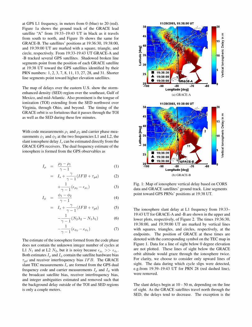
We define each CORS measurement to be within theenhancement or not based on whether the magnitude ofits equivalent vertical delay at 350 km shell height isgreater than a threshold of 12 m. Then, for a given choiceof altitude, the convex hull formed from the ionospherepierce points (IPPs) whose measurements were definedto be inside the enhancement has a certain area. As thealtitude increases, the area decreases, reaches a minimum,then increases again. Effectively, the enhancement region“comes into focus” at the altitude where the area is mini-mum and then “goes out of focus” as the altitude continuesto increase. By minimizing the area we hope to producethe high spatial rates of change of the ionosphere withthe model that were observed in the data. To distinguishbetween the SED and the TOI enhancements, we enforce aboundary at 35 degrees north latitude. The map in Figure 4shows the SED and TOI regions colored black and outlinedin white. For the TOI region, we define a center linerunning NNW-SSE that represents the axis through thecentroid. For the SED, we define a center line runningWNW-ESE through the centroid. These axes are depictedin white in Figure 4, and neglect earth-curvature effects.Recalling the asymmetry of the GRACE measurementsthrough the TOI, we shift its center line east one degree oflongitude from the position shown in Figure 4.

At each point of latitude and longitude, we assign a ver-tical electron density profile. For the background region,this electron density profile is based on the InternationalReference Ionosphere (IRI) 2000 model. The IRI model isa global climatological model that produces electron den-sity profiles for a specified place and time [2]. Since theenhancement regions are not predicted by the IRI modelalone, we test a range of Chapman functions. The Chapman

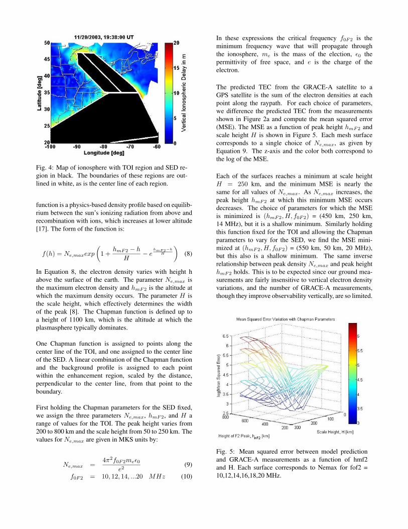
Fig. 4: Map of ionosphere with TOI region and SED re-gion in black. The boundaries of these regions are out-lined in white, as is the center line of each region.

function is a physics-based density profile based on equilib-rium between the sun’s ionizing radiation from above andrecombination with ions, which increases at lower altitude[17]. The form of the function is:

f(h) = Ne,maxexp

(1 +

hmF2 − h

H− e

hmF2−h

H

)(8)

In Equation 8, the electron density varies with height habove the surface of the earth. The parameter Ne,max isthe maximum electron density and hmF2 is the altitude atwhich the maximum density occurs. The parameter H isthe scale height, which effectively determines the widthof the peak [8]. The Chapman function is defined up toa height of 1100 km, which is the altitude at which theplasmasphere typically dominates.

One Chapman function is assigned to points along thecenter line of the TOI, and one assigned to the center lineof the SED. A linear combination of the Chapman functionand the background profile is assigned to each pointwithin the enhancement region, scaled by the distance,perpendicular to the center line, from that point to theboundary.

First holding the Chapman parameters for the SED fixed,we assign the three parameters Ne,max, hmF2, and H arange of values for the TOI. The peak height varies from200 to 800 km and the scale height from 50 to 250 km. Thevalues for Ne,max are given in MKS units by:

Ne,max =4π2f0F2meε0

e2(9)

f0F2 = 10, 12, 14, ...20 MHz (10)

In these expressions the critical frequency f0F2 is theminimum frequency wave that will propagate throughthe ionosphere, me is the mass of the election, ε0 thepermittivity of free space, and e is the charge of theelectron.

The predicted TEC from the GRACE-A satellite to aGPS satellite is the sum of the electron densities at eachpoint along the raypath. For each choice of parameters,we difference the predicted TEC from the measurementsshown in Figure 2a and compute the mean squared error(MSE). The MSE as a function of peak height hmF2 andscale height H is shown in Figure 5. Each mesh surfacecorresponds to a single choice of Ne,max, as given byEquation 9. The z-axis and the color both correspond tothe log of the MSE.

Each of the surfaces reaches a minimum at scale heightH = 250 km, and the minimum MSE is nearly thesame for all values of Ne,max. As Ne,max increases, thepeak height hmF2 at which this minimum MSE occursdecreases. The choice of parameters for which the MSEis minimized is (hmF2,H, f0F2) = (450 km, 250 km,14 MHz), but it is a shallow minimum. Similarly holdingthis function fixed for the TOI and allowing the Chapmanparameters to vary for the SED, we find the MSE mini-mized at (hmF2,H, f0F2) = (550 km, 50 km, 20 MHz),but this also is a shallow minimum. The same inverserelationship between peak density Ne,max and peak heighthmF2 holds. This is to be expected since our ground mea-surements are fairly insensitive to vertical electron densityvariations, and the number of GRACE-A measurements,though they improve observability vertically, are so limited.

Fig. 5: Mean squared error between model predictionand GRACE-A measurements as a function of hmf2and H. Each surface corresponds to Nemax for fof2 =10,12,14,16,18,20 MHz.

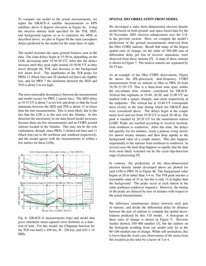
To compare our model to the actual measurements, wereplot the GRACE-A satellite measurements to GPSsatellites above 0 degrees elevation in Figure 6a. Usingthe electron density field specified for the TOI, SED,and background regions so as to minimize the MSE asdescribed above, we plot in Figure 6b the slant ionospheredelays predicted by the model for the same lines of sight.

The model recreates the same general features seen in thedata. The slant delays begin at 15-50 m, depending on theLOS, decreasing until 19:36:30 UT. After this the delaysincrease until they peak right around 19:38:00 UT as theytravel through the TOI, and decrease to the backgroundfew meter level. The amplitudes of the TOI peaks forPRNs 11 (black line) and 28 (dashed red lines) are slightlylow, and for PRN 7 the minimum between the SED andTOI is about 5 m too high.

The most noticeable discrepancy between the measurementand model occurs for PRN 2 (green line). The SED delayat 19:33 UT is about 7 m too low and drops so that the localminimum between the SED and TOI is about 15 m lowerthan the true measurements. This is most likely due to thefact that the LOS is to the east over the Atlantic. In thisdirection the uncertainty in our data-based model increasesbecause there are few measurements and no CORS groundstations located in the Atlantic. This may not be the soleexplanation, though, since PRNs 3 (dotted red line) and 11(black line) are to the northeast and southeast respectively,and the model agrees with the measurements to within afew meters for these LOSs.

Fig. 6: GRACE-A measurements (top) and model thatgives minimum mean squared error (bottom) as a func-tion of time. For this model, the Chapman function forthe TOI was hmf2 = 450 km, H - 250 km, and fof2 = 14MHz.

SPATIAL DECORRELATION FROM MODEL

We developed a static three-dimensional electron densitymodel based on both ground- and space-based data for the20 November 2003 electron enhancement over the U.S.in the previous section. Here, we compute the model’spredictions of the ground measurements observed fromthe Ohio CORS stations. Recall that many of the largestspatial rates of change, on the order of 350-400 mm ofdifferential delay per km of receiver separation, wereobserved from these stations [5]. A map of these stationsis shown in Figure 7. The nearest stations are separated by50-75 km.

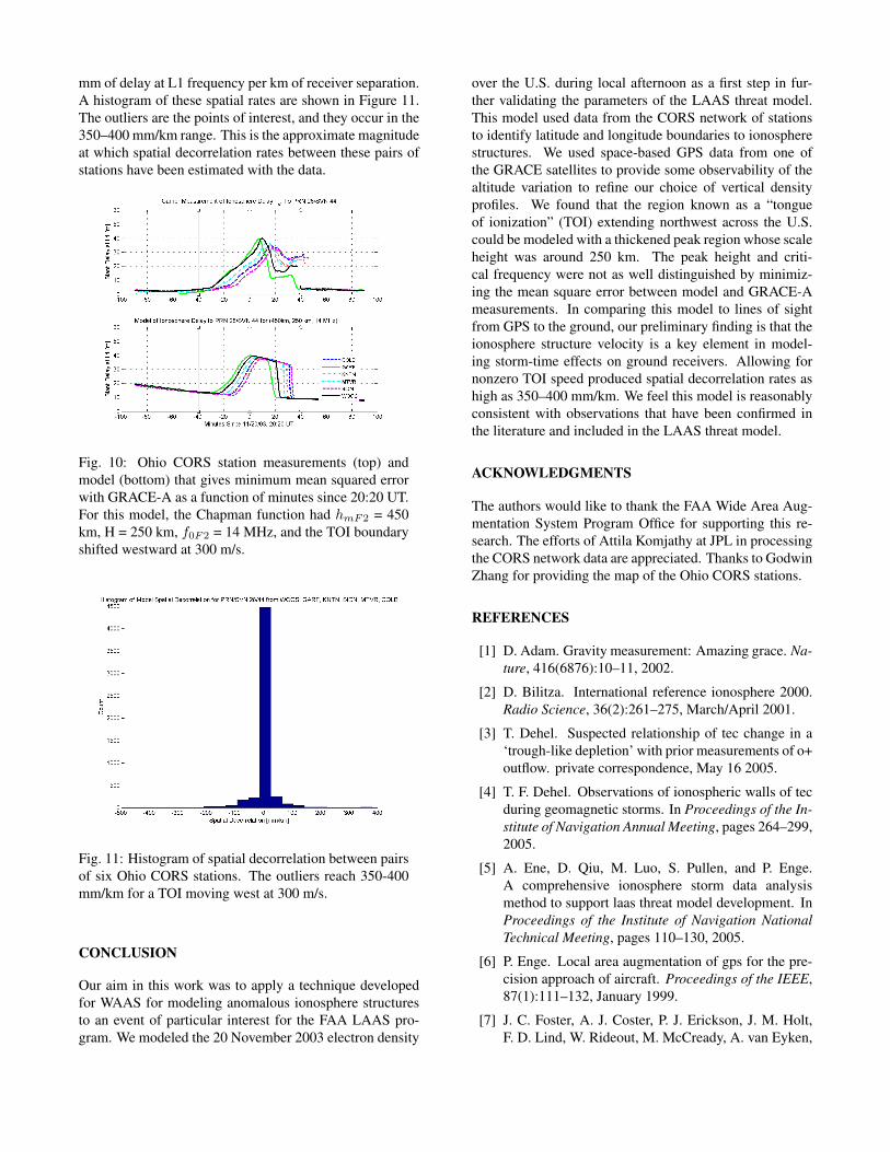
As an example of the Ohio CORS observations, Figure8a shows the JPL-processed, dual-frequency CORSmeasurements from six stations in Ohio to PRN 28 from18:50–21:50 UT. This is a three-hour time span, unlikethe ten-minute time window considered for GRACE.Vertical line segments at 19:40, 20:20, and 21:00 UT aremarked with a square, triangle, and circle respectively atthe endpoints. The vertical bar at 19:40 UT correspondsmost closely to the time during which the GRACE datawere considered above. The delays begin at the couplemeter level and rise from 19:50 UT to reach 30–40 m. Thepeak is reached by 20:30 UT for the easternmost stationGARF. Peaks are reached according to receiver location,from northeast to southwest. After this time, the delaysfall quickly for ten minutes, reach a plateau rising slowlyfor almost twenty minutes and then drop rapidly to thebackground value of a couple meters. This also happenssequentially to the stations from northeast to southwest. Inseveral cases the final drop happens so rapidly that the datawere most likely screened out by the cycle-slip-detectionstage of processing [9].

In contrast, the predictions of the three-dimensionalelectron density model developed above are plotted foreach LOS to PRN 28 in Figure 8b. The background valuebegins at 20 m rather than 3-4 m. The TOI peak reaches areasonable value of 35 m, but this is only 15 m higher thanthe background. The peaks occur at each station in thesame northeast-southwest sequence. However, the timingof the peaks are delayed by tens of minutes with respect tothe actual measurements.

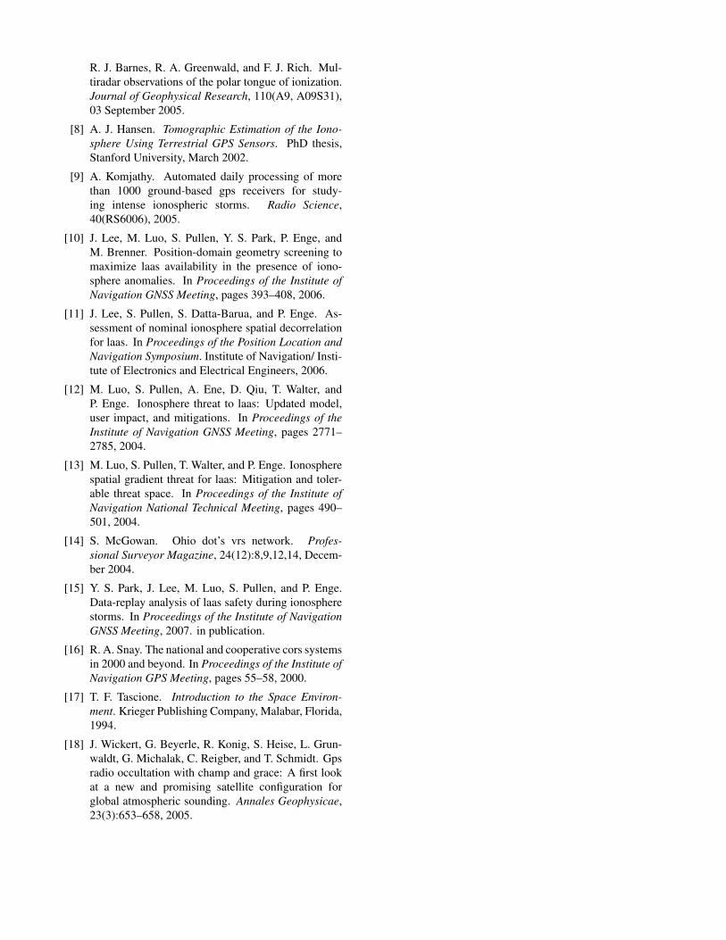
We difference simultaneous delays between each pairof stations, and divide the differential delay by distancebetween the pair of stations to compute the spatial decor-relation predicted by this 3-D model. A histogram ofthese rates of change is shown in Figure 9. Previousstudies showed 350–400 mm/km [3], but the outliers onthe histogram resulting from our model only lie in the80–100 mm/km rate of change. While still anomalous, thisis lower than the worst case observations of the storm fromthis location at this time by a factor of 3 or 4.

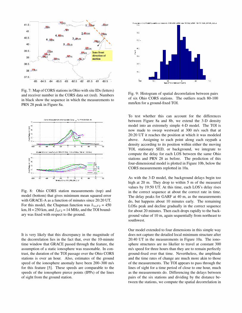
Fig. 7: Map of CORS stations in Ohio with site IDs (letters)and receiver number in the CORS data set (red). Numbersin black show the sequence in which the measurements toPRN 28 peak in Figure 8a.

Fig. 8: Ohio CORS station measurements (top) andmodel (bottom) that gives minimum mean squared errorwith GRACE-A as a function of minutes since 20:20 UT.For this model, the Chapman function was hmF2 = 450km, H = 250 km, and f0F2 = 14 MHz, and the TOI bound-ary was fixed with respect to the ground.

It is very likely that this discrepancy in the magnitude ofthe decorrelation lies in the fact that, over the 10-minutetime window that GRACE passed through the feature, theassumption of a static ionosphere was reasonable. In con-trast, the duration of the TOI passage over the Ohio CORSstations is over an hour. Also, estimates of the groundspeed of the ionosphere anomaly have been 200–300 m/sfor this feature [5]. These speeds are comparable to thespeeds of the ionosphere pierce points (IPPs) of the linesof sight from the ground station.

Fig. 9: Histogram of spatial decorrelation between pairsof six Ohio CORS stations. The outliers reach 80-100mm/km for a ground-fixed TOI.

To test whether this can account for the differencesbetween Figure 8a and 8b, we extend the 3-D densitymodel into an extremely simple 4-D model. The TOI isnow made to sweep westward at 300 m/s such that at20:20 UT it reaches the position at which it was modeledabove. Assigning to each point along each raypath adensity according to its position within either the movingTOI, stationary SED, or background, we integrate tocompute the delay for each LOS between the same Ohiostations and PRN 28 as before. The prediction of thisfour-dimensional model is plotted in Figure 10b, below theCORS measurements replotted in 10a.

As with the 3-D model, the background delays begin toohigh at 20 m. They drop to within 5 m of the measuredvalues by 19:50 UT. At this time, each LOS’s delay risesin the correct sequence at about the correct rate in time.The delay peaks for GARF at 40 m, as the measurementsdo, but happens about 10 minutes early. The remainingLOSs peak and decline gradually in the correct sequencefor about 20 minutes. Then each drops rapidly to the back-ground value of 10 m, again sequentially from northeast tosouthwest.

Our model extended to four dimensions in this simple waydoes not capture the detailed local minimum structure after20:40 UT in the measurements in Figure 10a. The iono-sphere structures are no likelier to travel at constant 300m/s speed for three hours than they are to remain perfectlyground-fixed over that time. Nevertheless, the amplitudeand the time rates of change are much more akin to thoseof the measurements. The TOI appears to pass through thelines of sight for a time period of close to one hour, muchas the measurements do. Differencing the delays betweenpairs of the six stations and dividing by the distance be-tween the stations, we compute the spatial decorrelation in

mm of delay at L1 frequency per km of receiver separation.A histogram of these spatial rates are shown in Figure 11.The outliers are the points of interest, and they occur in the350–400 mm/km range. This is the approximate magnitudeat which spatial decorrelation rates between these pairs ofstations have been estimated with the data.

Fig. 10: Ohio CORS station measurements (top) andmodel (bottom) that gives minimum mean squared errorwith GRACE-A as a function of minutes since 20:20 UT.For this model, the Chapman function had hmF2 = 450km, H = 250 km, f0F2 = 14 MHz, and the TOI boundaryshifted westward at 300 m/s.

Fig. 11: Histogram of spatial decorrelation between pairsof six Ohio CORS stations. The outliers reach 350-400mm/km for a TOI moving west at 300 m/s.

CONCLUSION

Our aim in this work was to apply a technique developedfor WAAS for modeling anomalous ionosphere structuresto an event of particular interest for the FAA LAAS pro-gram. We modeled the 20 November 2003 electron density

over the U.S. during local afternoon as a first step in fur-ther validating the parameters of the LAAS threat model.This model used data from the CORS network of stationsto identify latitude and longitude boundaries to ionospherestructures. We used space-based GPS data from one ofthe GRACE satellites to provide some observability of thealtitude variation to refine our choice of vertical densityprofiles. We found that the region known as a “tongueof ionization” (TOI) extending northwest across the U.S.could be modeled with a thickened peak region whose scaleheight was around 250 km. The peak height and criti-cal frequency were not as well distinguished by minimiz-ing the mean square error between model and GRACE-Ameasurements. In comparing this model to lines of sightfrom GPS to the ground, our preliminary finding is that theionosphere structure velocity is a key element in model-ing storm-time effects on ground receivers. Allowing fornonzero TOI speed produced spatial decorrelation rates ashigh as 350–400 mm/km. We feel this model is reasonablyconsistent with observations that have been confirmed inthe literature and included in the LAAS threat model.

ACKNOWLEDGMENTS

The authors would like to thank the FAA Wide Area Aug-mentation System Program Office for supporting this re-search. The efforts of Attila Komjathy at JPL in processingthe CORS network data are appreciated. Thanks to GodwinZhang for providing the map of the Ohio CORS stations.

REFERENCES

[1] D. Adam. Gravity measurement: Amazing grace. Na-ture, 416(6876):10–11, 2002.

[2] D. Bilitza. International reference ionosphere 2000.Radio Science, 36(2):261–275, March/April 2001.

[3] T. Dehel. Suspected relationship of tec change in a‘trough-like depletion’ with prior measurements of o+outflow. private correspondence, May 16 2005.

[4] T. F. Dehel. Observations of ionospheric walls of tecduring geomagnetic storms. In Proceedings of the In-stitute of Navigation Annual Meeting, pages 264–299,2005.

[5] A. Ene, D. Qiu, M. Luo, S. Pullen, and P. Enge.A comprehensive ionosphere storm data analysismethod to support laas threat model development. InProceedings of the Institute of Navigation NationalTechnical Meeting, pages 110–130, 2005.

[6] P. Enge. Local area augmentation of gps for the pre-cision approach of aircraft. Proceedings of the IEEE,87(1):111–132, January 1999.

[7] J. C. Foster, A. J. Coster, P. J. Erickson, J. M. Holt,F. D. Lind, W. Rideout, M. McCready, A. van Eyken,

R. J. Barnes, R. A. Greenwald, and F. J. Rich. Mul-tiradar observations of the polar tongue of ionization.Journal of Geophysical Research, 110(A9, A09S31),03 September 2005.

[8] A. J. Hansen. Tomographic Estimation of the Iono-sphere Using Terrestrial GPS Sensors. PhD thesis,Stanford University, March 2002.

[9] A. Komjathy. Automated daily processing of morethan 1000 ground-based gps receivers for study-ing intense ionospheric storms. Radio Science,40(RS6006), 2005.

[10] J. Lee, M. Luo, S. Pullen, Y. S. Park, P. Enge, andM. Brenner. Position-domain geometry screening tomaximize laas availability in the presence of iono-sphere anomalies. In Proceedings of the Institute ofNavigation GNSS Meeting, pages 393–408, 2006.

[11] J. Lee, S. Pullen, S. Datta-Barua, and P. Enge. As-sessment of nominal ionosphere spatial decorrelationfor laas. In Proceedings of the Position Location andNavigation Symposium. Institute of Navigation/ Insti-tute of Electronics and Electrical Engineers, 2006.

[12] M. Luo, S. Pullen, A. Ene, D. Qiu, T. Walter, andP. Enge. Ionosphere threat to laas: Updated model,user impact, and mitigations. In Proceedings of theInstitute of Navigation GNSS Meeting, pages 2771–2785, 2004.

[13] M. Luo, S. Pullen, T. Walter, and P. Enge. Ionospherespatial gradient threat for laas: Mitigation and toler-able threat space. In Proceedings of the Institute ofNavigation National Technical Meeting, pages 490–501, 2004.

[14] S. McGowan. Ohio dot’s vrs network. Profes-sional Surveyor Magazine, 24(12):8,9,12,14, Decem-ber 2004.

[15] Y. S. Park, J. Lee, M. Luo, S. Pullen, and P. Enge.Data-replay analysis of laas safety during ionospherestorms. In Proceedings of the Institute of NavigationGNSS Meeting, 2007. in publication.

[16] R. A. Snay. The national and cooperative cors systemsin 2000 and beyond. In Proceedings of the Institute ofNavigation GPS Meeting, pages 55–58, 2000.

[17] T. F. Tascione. Introduction to the Space Environ-ment. Krieger Publishing Company, Malabar, Florida,1994.

[18] J. Wickert, G. Beyerle, R. Konig, S. Heise, L. Grun-waldt, G. Michalak, C. Reigber, and T. Schmidt. Gpsradio occultation with champ and grace: A first lookat a new and promising satellite configuration forglobal atmospheric sounding. Annales Geophysicae,23(3):653–658, 2005.