1

Modeling Temperature in a Breast Cancer Tumor for

Ultrasound-Based Hyperthermia Treatment

Brian Ho

Kanmani Kannayiram

Ryan Tam

Harrison Yang

2

Introduction

Hyperthermia, also called thermal therapy or thermotherapy, is a type of cancer treatment in

which body tissue is exposed to high temperatures of up to 113 ºF to damage and/or kill cancer

cells. Research has shown that high temperatures can damage and kill cancer cells with minimal

injury to the surrounding tissue, making it much safer than traditional treatment therapies.

Hyperthermia is most commonly used in conjunction with other forms of cancer therapy, such

as radiation and chemotherapy. Furthermore, many clinical studies show that high temperature

hyperthermia alone can be used for selective tissue destruction as an alternative to

conventional invasive surgery. Due to the heterogeneous and dynamic properties of tissues,

including blood perfusion and metabolic heat generation, it is important to present models of

the temperature change during the treatment of tumors. The method of hyperthermia we will

be looking at is local hyperthermia, in which heat is applied to a small area using a focused

ultrasound beam. This will be an external approach where the applicator is positioned around

the appropriate region.

The effectiveness of hyperthermia depends greatly on the temperature achieved during the

treatment. Another important factor is the duration of the treatment and temperature of the

surrounding tissue. This application can easily be done, but monitoring of the temperature

requires invasive needles with tiny thermometers to be inserted in the treatment area to

ensure that the desired temperature is reached and the surrounding tissue will not be

damaged. Imaging techniques such as CT scans are also required and can be expensive to use

for clinical study purposes. Thus, a mathematical model is better used for understanding the

temperature profile of the tumor.

Problem Formulation, Assumptions and Values

In this study, we will be modeling the heat transfer of an ultrasound beam on a breast cancer

tumor. This is more commonly known as a hyperthermia treatment for cancer. Literature has

described that in order to have an effective treatment, resulting in a reduction of tumor size,

the tumor must reach a temperature of approximately 45 ºC. To simply our model, we will be

analyzing the tumor as a perfect sphere with radius R = 1 cm = 0.01 m. We will also be

simplifying the ultrasound beam to be perfectly focused, in other words, the beam only applies

heat at a point in the center tumor and any other heat energy from the beam is negligible.

For the purposes of this model we will be utilizing the Pennes bioheat equation (which is the

general heat diffusion equation with additional terms for perfusion of blood and metabolic

heat), in spherical coordinates, as follows:

=

(

)+qp+

3

Where is density of the tumor, Cp is the heat capacity of the tissue, k is thermal conductivity

of tissue and is the metabolic heat term (or heat that the tumor generates from its

metabolic processes). qp is defined as heat perfusion or the heat that is carried away from the

tumor site by arterial blood flow and is defined as:

where = perfusion rate

of blood, = arterial temperature, T = local tissue temperature, = density of blood and

= heat capacity of blood. This means that the temperature profile with respect to time is

dependent on the diffusivity of heat through the tumor as well as how much heat is exchanged

through the arteries and metabolic heat generation.

In this situation, we will be neglecting the qp (the heat perfusion term) in an attempt to simplify

the model. This means that we will be modeling the two remaining scenarios: the basic scenario

without considering metabolic heat (Scenario 1) and then one considering the metabolic heat

term (Scenario 2). This means that the equation to be modeled is reduced to (after dividing by

on both sides and simplifying):

= D

) [Scenario 1]

= D

) +

[Scenario 2]

Where D =

We will analytically solve these equations to get the two respective temperature profiles. The

boundary conditions applied are:

= 45 [Temperature at the center of the tumor, applied point source

temperature]

= 37 [Temperature at the boundary of the tumor, physiological temperature]

And the initial condition used is:

37 [Initial temperature of tumor at time t = 0, physiological temperature]

The physiological constant values used in the model (derived from literature) are:

= 0.42

[Thermal conductivity of tumor]

= 920

[Density of tumor]

Cp = 3600

[Heat capacity of tumor]

4

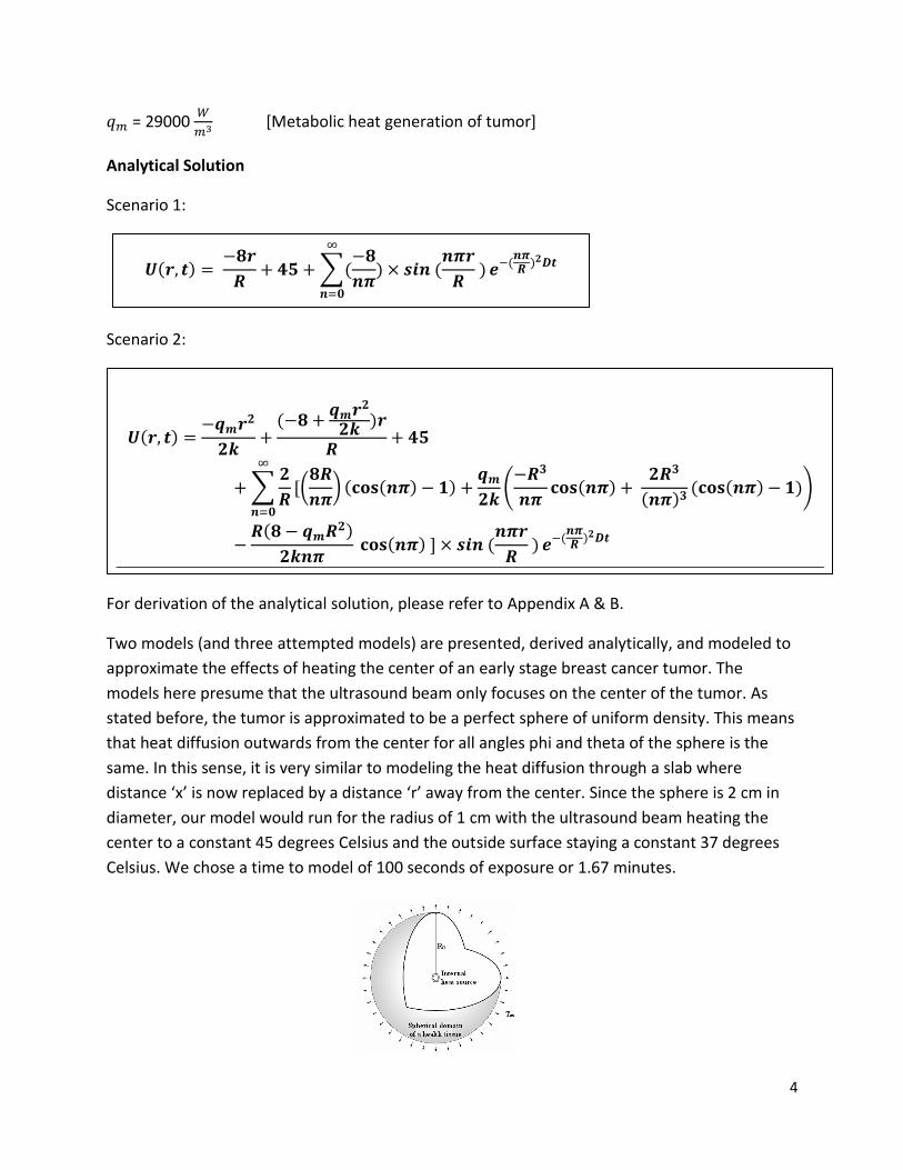
= 29000

[Metabolic heat generation of tumor]

Analytical Solution

Scenario 1:

Scenario 2:

For derivation of the analytical solution, please refer to Appendix A & B.

Two models (and three attempted models) are presented, derived analytically, and modeled to

approximate the effects of heating the center of an early stage breast cancer tumor. The

models here presume that the ultrasound beam only focuses on the center of the tumor. As

stated before, the tumor is approximated to be a perfect sphere of uniform density. This means

that heat diffusion outwards from the center for all angles phi and theta of the sphere is the

same. In this sense, it is very similar to modeling the heat diffusion through a slab where

distance ‘x’ is now replaced by a distance ‘r’ away from the center. Since the sphere is 2 cm in

diameter, our model would run for the radius of 1 cm with the ultrasound beam heating the

center to a constant 45 degrees Celsius and the outside surface staying a constant 37 degrees

Celsius. We chose a time to model of 100 seconds of exposure or 1.67 minutes.

5

First Model

The first model shows the heating profile of a tumor in an isolated system, which means there

are no external factors to consider. This is to show the diffusion of heat through the tumor if no

means of heat loss were present.

Figure 1: Temperature profile for a

tumor isolated from the body, for

100 seconds.

The temperature at the center of

the tumor is a constant 45 .

Overtime the temperature of the

tumor gradually increases.

Figure 2: Temperature profile for a

tumor isolated from the body, for

10000 seconds.

The temperature throughout the

tumor is higher than the previous

model which makes sense since a

longer time is allotted for the tumor

to heat.

6

Figure 3: Effect of time on the

analytical solution.

Confirms that as time goes on, the

temperature of the tumor increases

gradually with time.

Second Model

The second model is the same as the first but takes into account the metabolic heat generated

by the cells themselves. The metabolic heat constant we used is 29000

. The expectation is

that the heat generated by the living tissue would have an additive effect to the external heat

generated by the ultrasound. So the hypothesis would be that the tumor would reach an overall

higher temperature and also heat at a faster rate.

Figure 4: Temperature profile for a

tumor in the body, taking into

account metabolic heat generated,

for 100 seconds.

The heat source at 45 is heats the

tumor to a different gradient as the

isolated tumor, but still increases

the overall temperature.

7

Figure 5: Temperature profile for a

tumor in the body, taking into

account metabolic heat generated,

for 10000 seconds.

The overall temperature of the

tumor improves with an increased

duration of treatment, as observed

by the final temperature profile

compared to the previous figure.

Figure 6: Effect of varying exposure

times on the analytical solution.

As expected, at time = 100 seconds,

it can be seen that the temperature

is higher at all points throughout

the radius of the spherical tumor

model. Although for lower time

models this is not always the case.

Comparing Figure 3 to Figure 6, perhaps the most unusual observation from these plots is that

with the metabolic heat term introduced into the system, the temperature is lower for shorter

exposure periods to the ultrasound. We originally expected a uniform shift upwards but this is

only seen at the final time point of 100 seconds. We can only observe that the introduction of

8

metabolic heat affects the effectiveness of the ultrasound beam in some way that the

temperature is lower than without the additional heat generation.

Conclusion

Ultrasound presents a new way to treat cancerous tumors by hyperthermia, or heating the

tumor, with minimal damage to surrounding tissues. Most normal tissues are not damaged

during hyperthermia if the temperature remains under 43.9 ºC, however, due to regional

differences in tissue characteristics, higher temperatures may occur in various spots that result

in burns, blisters, discomfort, or pain. Ultrasound reduces the damage to surrounding tissue by

having a less pronounced effect on less dense tissue.

Our model shows that for a relatively small tumor (2 cm in diameter) and a point heat source

set at 45 ºC, only a small part in the interior of the tumor would be damaged and/or destroyed

within a period of approximately 100 seconds. However, it is good to note that this is a

simplified model that is not taking into account arterial heat perfusion. The selected heat

source temperature is a relatively low and to achieve better results, a point heat source at a

higher temperature would be more effective at generating a sufficient temperature throughout

the tumor faster. However, this comes at the risk of damaging the surrounding tissue even with

the relative safety of ultrasound.

In conclusion, the results of this very simplified model form a basic foundation for a better

understanding for the use of ultrasound for hyperthermia treatment and how heat diffusion

works in tumors in general. To further our understanding of the effect of ultrasound, more

complex and extensive analytical methods including all aspects of heat conduction, perfusion

and metabolic heat terms should be considered to form a more complete picture of the

phenomena that occurs in vivo when ultrasound is applied.

9

References

Gutierrez, Gustavo. "Study of the Bioheat Equation with a Spherical Heat Source for Local

Magnetic Hyperthermia." XVI Congress on Numerical Methods and Their Applications (2007): n.

pag. Web. 17 Oct. 2012.

"National Cancer Institute." Hyperthermia in Cancer Treatment -. N.p., n.d. Web. 17 Oct. 2012.

<http://www.cancer.gov/cancertopics/factsheet/Therapy/hyperthermia>.

Hassan, Osama et. al. "Modeling of Ultrasound Hyperthermia Treatment of Breast Tumors."

26th National Radio Science Conference (2009): n. pag. 17 Mar. 2009. Web. 17 Oct. 2012.

Shih, Tzu-Ching et. al. "Analytical Analysis of the Pennes Bioheat Transfer Equation with

Sinusoidal Heat flux Condition on Skin Surface." Medical Engineering & Physics (2007): n. pag.

Web. 17 Oct. 2012.

Umadevi, V. et. al "Framework for Estimating Tumour Parameters Using Thermal Imaging."

Indian Journal of Medical Research (2011): n. pag. Web. 17 Oct. 2012.

Special Thanks to:

Dr. Jakob Nebeker for providing the inspiration for this project

Dr. Guy Cohen for assistance with analytical methods

10

Appendix A: Analytical Solution For Model Without External

Heat Sources

Assuming no perfusion of heat from the tumor and blood ( , and no metabolic heat

released , the simplified diffusion equation is attained, where u is temperature (in degrees

Celsius) and t is time (in seconds) and r is the distance (in meters):

The complete solution is based on the summation of the homogeneous ( ) and steady state

terms ( ):

(0)

The boundary conditions are determined to be:

Initial Condition #1: U(r,0) = 37 C

Boundary Condition #1: U(0,t) = 45 C

Boundary Condition #2: U(R,t) = 37 C

These boundary conditions reflect the fact that the tumor temperature is initially at

physiological body temperature, which is 37 C. The ultrasound laser heats the center of the

tumor, at r=0, to 45 C, and that comprises our first boundary condition. The edge of the

tumor at r=R is modeled to be at body temperature, 37 C.

Solve the steady state term ( ) and plug boundary conditions to it:

=

;

(1)

Rescale to homogeneous initial and boundary conditions:

New IC:

(2)

New BCs:

11

Use separation of variables:

(3)

Upon solving, this gets (4)

And for cases of (other cases proven to be trivial solutions) the characteristic equation of

is attained. Plugging in the boundary conditions yields

and

(5)

Plug (5) and (4) to (3) yields

(6)

Where

(7)

Plug in (2) to (7) and integrate the term, and replug B to (6) to get the final

(8)

And replug (8) and (1) to (0) to get the complete temperature profile:

12

Appendix B: Analytical Solution For Model with Addition of

Metabolic Heat Term

Assuming no perfusion of heat from the tumor and blood ( , and no metabolic heat released

, the simplified diffusion equation is attained, where u is temperature (in degrees Celsius)

and t is time (in seconds) and r is the distance (in meters):

The complete solution is based on the summation of the homogeneous ( ) and steady state

terms ( ):

(0)

The boundary conditions, as in Appendix A, are determined to be:

Initial Condition #1: U(r,0) = 37 C

Boundary Condition #1: U(0,t) = 45 C

Boundary Condition #2: U(R,t) = 37 C

Solve the steady state term ( ) and plug boundary conditions to it:

=

; know

so solve:

(1)

Rescale to homogeneous initial and boundary conditions:

New IC:

(2)

New BCs:

13

Use separation of variables:

(3)

Upon solving, this gets (4)

And for cases of (other cases proven to be trivial solutions) the characteristic equation of

is attained. Plugging in the boundary conditions yields

and

(5)

Plug (5) and (4) to (3) yields

(6)

Where

(7)

Plug in (2) to (7) and integrate the term, and replug B to (6) to get the final

(8)

And replug (8) and (1) to (0) to get the complete temperature profile:

14

Appendix C: MATLAB Code

Part I: MATLAB Code For Model Without External Heat

Sources

%Ryan Tam %Ultrasound beam focused on center of spherical tumor %Modeled outside of tumor (length R away from the tumor on all sides) at %body temperature, 37 degrees Celsius %Assume no heat generation or perfusion in idealized model, but ultrasound

beam %heats the center of the tumor at 45 degrees. Initial temperature is 37 %degrees throughout sphere (only affected by the body temperature).

clear all close all clc

%tissue refers to the tumor; tissue constants K_tissue= 0.42; %in W/m, thermal conductivity of the tissue density_tissue = 920; %in kg/m^3, density of the tissue specificheat_tissue= 3600; %in J/kg*degrees Celsius, specific heat of tissue,

3600 is another option from another source diffusivity_tissue=K_tissue/(density_tissue*specificheat_tissue);

radius_tumor=0.01; %1 cm, converted to m; because tumor diameter is 2 cm,

which is a early stage 2 breast cancer tumor r_distance=radius_tumor*2;

time_total=100; %100 seconds dr=r_distance/10; %step size in for r distance (along radius of tumor) dt=0.1; %step size in the t direction (time in seconds)

rmesh=0:dr:r_distance; %iterates to 2X the radius of the tumor, past the

tumor's surface and a distance r from the tumor surface tmesh=0:dt:time_total; %iterates up to 100 seconds rskip=2; tskip=2;

number_iterations=10;

nr=length(rmesh); nt=length(tmesh);

V=zeros(nt,nr);

for i=1:nr for j=1:nt

15

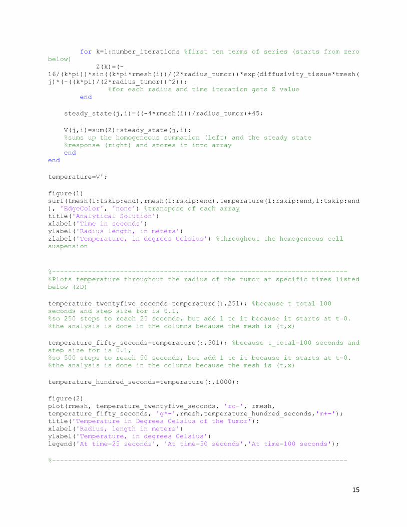
for k=1:number_iterations %first ten terms of series (starts from zero

below) Z(k)=(-

16/(k*pi))*sin((k*pi*rmesh(i))/(2*radius_tumor))*exp(diffusivity_tissue*tmesh(

j)*(-((k*pi)/(2*radius_tumor))^2)); %for each radius and time iteration gets Z value end

steady_state(j,i)=((-4*rmesh(i))/radius_tumor)+45;

V(j,i)=sum(Z)+steady_state(j,i); %sums up the homogeneous summation (left) and the steady state %response (right) and stores it into array end end

temperature=V';

figure(1) surf(tmesh(1:tskip:end),rmesh(1:rskip:end),temperature(1:rskip:end,1:tskip:end

), 'EdgeColor', 'none') %transpose of each array title('Analytical Solution') xlabel('Time in seconds') ylabel('Radius length, in meters') zlabel('Temperature, in degrees Celsius') %throughout the homogeneous cell

suspension

%-------------------------------------------------------------------------- %Plots temperature throughout the radius of the tumor at specific times listed

below (2D)

temperature_twentyfive_seconds=temperature(:,251); %because t_total=100

seconds and step size for is 0.1, %so 250 steps to reach 25 seconds, but add 1 to it because it starts at t=0. %the analysis is done in the columns because the mesh is (t,x)

temperature_fifty_seconds=temperature(:,501); %because t_total=100 seconds and

step size for is 0.1, %so 500 steps to reach 50 seconds, but add 1 to it because it starts at t=0. %the analysis is done in the columns because the mesh is (t,x)

temperature_hundred_seconds=temperature(:,1000);

figure(2) plot(rmesh, temperature_twentyfive_seconds, 'ro-', rmesh,

temperature_fifty_seconds, 'g*-',rmesh,temperature_hundred_seconds,'m+-'); title('Temperature in Degrees Celsius of the Tumor'); xlabel('Radius, length in meters') ylabel('Temperature, in degrees Celsius') legend('At time=25 seconds', 'At time=50 seconds','At time=100 seconds');

%--------------------------------------------------------------------------

16

Part II: MATLAB Code For Model with Addition of Metabolic

Heat Term

%Ryan Tam %Ultrasound beam focused on center of spherical tumor %Modeled outside of tumor (length R away from the tumor on all sides) at %body temperature, 37 degrees Celsius %Assume no heat generation or perfusion in idealized model, but ultrasound

beam %heats the center of the tumor at 45 degrees. Initial temperature is 37 %degrees throughout sphere (only affected by the body temperature).

clear all close all clc

%tissue refers to the tumor; tissue constants K_tissue= 0.42; %in W/m, thermal conductivity of the tissue density_tissue = 920; %in kg/m^3, density of the tissue specificheat_tissue= 3600; %in J/kg*degrees Celsius, specific heat of tissue,

3600 is another option from another source diffusivity_tissue=K_tissue/(density_tissue*specificheat_tissue);

%blood constants perfusion_blood=9*10^-6; %tumor perfusion rate, in L/s density_blood=1000; %1000 kg/m^3 specificheat_blood=3000; %in J/kg*degrees Celsius, blood_constant=(perfusion_blood*density_blood*specificheat_blood)/K_tissue;

temperature_arteries=37; %given arterial temperature, degrees Celsius

radius_tumor=0.01; %1 cm, converted to m; because tumor diameter is 2 cm,

which is a early stage 2 breast cancer tumor r_distance=radius_tumor*2;

time_total=100; %100 seconds dr=r_distance/10; %step size in for r distance (along radius of tumor) dt=0.1; %step size in the t direction (time in seconds)

rmesh=0:dr:r_distance; %iterates to 2X the radius of the tumor, past the

tumor's surface and a distance r from the tumor surface tmesh=0:dt:time_total; %iterates up to 100 seconds rskip=2; tskip=2;

number_iterations=10;

nr=length(rmesh); nt=length(tmesh);

V=zeros(nt,nr);

17

for i=1:nr for j=1:nt for k=1:number_iterations %first ten terms of series (starts from zero

below)

first_term=(-8+temperature_arteries)*((-

2*radius_tumor)/(k*pi))*(cos(k*pi)-1);

second_term_one=(1/(2*sqrt(blood_constant))*sin((k*pi*sqrt(blood_constant))/(2

*radius_tumor))*cosint((k*pi*(2*radius_tumor-

sqrt(blood_constant)))/(2*radius_tumor)));

second_term_two=sin((k*pi*sqrt(blood_constant))/(2*radius_tumor))*cosint((k*pi

*(2*radius_tumor+sqrt(blood_constant)))/(2*radius_tumor));

second_term_three=cos((k*pi*sqrt(blood_constant))/(2*radius_tumor))*(sinint((k

*pi*(sqrt(blood_constant)-

2*radius_tumor))/(2*radius_tumor))+sinint((k*pi*(2*radius_tumor+sqrt(blood_con

stant)))/(2*radius_tumor)));

second_term_four=(1/(2*sqrt(blood_constant))*sin((k*pi*sqrt(blood_constant))/(

2*radius_tumor))*cosint((k*pi*(-sqrt(blood_constant)))/(2*radius_tumor)));

second_term_five=sin((k*pi*sqrt(blood_constant))/(2*radius_tumor))*cosint((k*p

i*(sqrt(blood_constant)))/(2*radius_tumor));

second_term_six=cos((k*pi*sqrt(blood_constant))/(2*radius_tumor))*(sinint((k*p

i*(sqrt(blood_constant)))/(2*radius_tumor))+sinint((k*pi*(sqrt(blood_constant)

))/(2*radius_tumor)));

second_term=(blood_constant*temperature_arteries)*(second_term_one+second_term

_two-second_term_three-second_term_four-second_term_five+second_term_six);

third_term=((8-temperature_arteries-

((blood_constant*temperature_arteries)/((4*radius_tumor^2)-

blood_constant)))/(2*radius_tumor))*((-4*cos(k*pi)*radius_tumor^2)/(k*pi));

b_term=(1/radius_tumor)*(first_term+second_term+third_term);

Z(k)=b_term*sin((k*pi*rmesh(i))/(2*radius_tumor))*exp(diffusivity_tissue*tmesh

(j)*(-((k*pi)/(2*radius_tumor))^2)); %for each radius and time iteration gets Z value end

steady_state(j,i)=(45-temperature_arteries)+((-

blood_constant*temperature_arteries)/(((rmesh(i))^2)-

blood_constant))+(rmesh(i)/(2*radius_tumor))*(-

8+temperature_arteries+((blood_constant*temperature_arteries)/((4*radius_tumor

^2)-blood_constant)));

V(j,i)=sum(Z)+steady_state(j,i);

18

%sums up the homogeneous summation (left) and the steady state %response (right) and stores it into array end end

temperature=V';

figure(1) surf(tmesh(1:tskip:end),rmesh(1:rskip:end),temperature(1:rskip:end,1:tskip:end

), 'EdgeColor', 'none') %transpose of each array title('Analytical Solution, with Heat Perfusion to Arteries') xlabel('Time in seconds') ylabel('Radius length, in meters') zlabel('Temperature, in degrees Celsius') %throughout the homogeneous cell

suspension

%-------------------------------------------------------------------------- %Plots temperature throughout the radius of the tumor at specific times listed

below (2D)

temperature_twentyfive_seconds=temperature(:,251); %because t_total=100

seconds and step size for is 0.1, %so 250 steps to reach 25 seconds, but add 1 to it because it starts at t=0. %the analysis is done in the columns because the mesh is (t,x)

temperature_fifty_seconds=temperature(:,501); %because t_total=100 seconds and

step size for is 0.1, %so 500 steps to reach 50 seconds, but add 1 to it because it starts at t=0. %the analysis is done in the columns because the mesh is (t,x)

temperature_hundred_seconds=temperature(:,1000);

figure(2) plot(rmesh, temperature_twentyfive_seconds, 'ro-', rmesh,

temperature_fifty_seconds, 'g*-',rmesh,temperature_hundred_seconds,'m+-'); title('Temperature in Degrees Celsius of the Tumor'); xlabel('Radius, length in meters') ylabel('Temperature, in degrees Celsius') legend('At time=5 seconds', 'At time=25 seconds', 'At time=50 seconds','At

time=100 seconds');

%--------------------------------------------------------------------------