Modeling Steady Sea Water Intrusion with Single-Density Groundwater Codes

Modeling Steady Sea Water Intrusionwith Single-Density Groundwater Codesby Mark Bakker1 and Frans Schaars2

AbstractSteady interface flow in heterogeneous aquifer systems is simulated with single-density groundwater codes by

using transformed values for the hydraulic conductivity and thickness of the aquifers and aquitards. For example,unconfined interface flow may be simulated with a transformed model by setting the base of the aquifer tosea level and by multiplying the hydraulic conductivity with 41 (for sea water density of 1025 kg/m3). Similartransformations are derived for unconfined interface flow with a finite aquifer base and for confined multi-aquiferinterface flow. The head and flow distribution are identical in the transformed and original model domains. Thelocation of the interface is obtained through application of the Ghyben-Herzberg formula. The transformed problemmay be solved with a single-density code that is able to simulate unconfined flow where the saturated thicknessis a linear function of the head and, depending on the boundary conditions, the code needs to be able to simulatedry cells where the saturated thickness is zero. For multi-aquifer interface flow, an additional requirement is thatthe code must be able to handle vertical leakage in situations where flow in an aquifer is unconfined while thereis also flow in the aquifer directly above it. Specific examples and limitations are discussed for the application ofthe approach with MODFLOW. Comparisons between exact interface flow solutions and MODFLOW solutionsof the transformed model domain show good agreement. The presented approach is an efficient alternative torunning transient sea water intrusion models until steady state is reached.

IntroductionSea water intrusion in coastal aquifers may be

simulated with computer codes that combine groundwaterflow, contaminant transport, and density effects, suchas SEAWAT (Langevin et al. 2008), SUTRA (Voss andProvost 2010), and FEFLOW (Diersch and Kolditz 2002).Application of these codes requires a three-dimensionaldiscretization of the aquifer system to keep track ofthe density distribution, and sufficiently small time stepsto keep numerical dispersion at bay. As a result, the

1Corresponding author: Water Resources Section, Faculty ofCivil Engineering and Geosciences, Delft University of Technology,Delft, The Netherlands; [email protected]

2Artesia, Schoonhoven, The Netherlands; [email protected]

Received November 2011, accepted May 2012.© 2012, The Author(s)Ground Water © 2012, National Ground Water Association.doi: 10.1111/j.1745-6584.2012.00955.x

computational effort involved is large, especially whensimulations are run until steady-state conditions arereached.

Alternatively, sea water intrusion may be simulatedwith the SWI package for MODFLOW (Bakker andSchaars 2005), which is based on the Dupuit formulationfor modeling sea water intrusion presented by Bakker(2003). SWI does not require a vertical discretization ofan aquifer, as it applies the Dupuit approximation for flowwithin an aquifer. The evolution of the salinity distributionthrough time is computed by application of continuityof flow for water of different salinities, while neglectingany additional mixing of different salinities during thesimulation. As a result, SWI simulations require muchless computational effort, typically at least three ordersof magnitude less than the aforementioned codes thatsolve the combined flow and transport equations (Bakkeret al. 2004; Dausman et al. 2010). Dausman et al. (2010)investigated the differences between transient sea water

NGWA.org GROUND WATER 1

intrusion simulations with SWI (in interface mode) andSEAWAT. They concluded that results were similar exceptfor cases where the dispersion across the interface islarge, when the vertical hydraulic conductivity is lessthan 1% of the horizontal hydraulic conductivity, and insome cases of inversion. For simulations where SWI andSEAWAT results diverged, the interface simulated withSWI tended to be more landward than the transition zonesimulated with SEAWAT. Similarly, Pool and Carrera(2011) showed that the transition zone is wider andmore seaward than an interface when larger transversedispersivity values are used.

Final steady-state conditions are of interest in largeregional models that include a coastal boundary inorder to estimate pre-development conditions in anaquifer, to design well fields in coastal aquifers, or toevaluate proposed designs to limit sea water intrusion.For such simulations, it is often sufficient to simulateflow in an aquifer as interface flow (Cheng et al. 2000;Mantoglou 2003). Codes that combine groundwater flowand transport are not well suited to simulate interfaceflow as requirements for vertical discretization and timesteps lead to prohibitively large computation times. SWIis better suited to compute the steady position of theinterface, but it is inconvenient as it requires specificationof the initial interface position as well as some algorithm-specific parameters. In addition, it may take a significantsimulation time before steady state is reached.

The steady position of an interface between freshand salt water may be computed from the head withthe well-known Ghyben-Herzberg equation (Bear 1972;Strack 1989; Fitts 2002). Application of the potentialintroduced by Strack (1976) is a common approach forthe simulation of steady interface flow in a single aquifer.The Strack potential is implemented in the analyticelement codes Gflow (www.haitjema.com) and AnAqSym(www.fittsgeosolutions.com), which allow for modelingof interface flow in single aquifers. Strack’s potentialis applicable to aquifers with piecewise homogeneousproperties. Although it is, in theory, applicable to multi-aquifer systems, it is inconvenient as it leads to a systemof linked, nonlinear differential equations (Sikkema andVan Dam 1982; Bakker 2006).

For simulation of steady interface flow in multi-aquifersystems with variable properties, it seems necessary toapply a numerical solution technique. The objective of thispaper is to present an approach to simulate the steady-stateposition of the interface in a heterogeneous multi-aquifersystem with a standard single-density groundwater code.At steady state, the salt water is stagnant and the saltwater head is constant everywhere in the salt water zone.No sinks or sources may be present in the salt water. Thesimplest case of unconfined interface flow is discussedfirst, after which the approach is extended to unconfinedinterface flow with a finite base, and to interface flow inmulti-aquifer systems. A number of examples are pre-sented and solved using MODFLOW (Harbaugh et al.2000; Harbaugh 2005). The limitations of the approachare discussed.

h

zs

D H

sealevel

datumx

z

salt

flowingfresh water

h

zs

D H

sealevel

datumx

z

zb

salt

flowingfresh water

(a)

(b)

interface toe

Figure 1. (a) Unconfined interface flow and (b) Combinedunconfined interface flow and unconfined flow.

Steady Unconfined Interface Flow in a DeepAquifer

Consider steady unconfined interface flow in a deepaquifer so that the interface does not touch the bottomof the aquifer anywhere, as illustrated in Figure 1a. ACartesian x, y, z coordinate system is adopted with the z-axis pointing vertically upward. The origin of the z-axisis at an arbitrary reference level referred to as the datum.Heads and elevations are measured with respect to thedatum; the elevation of sea level is zs . The salt water is atrest. The density of the fresh water is ρf and of the saltwater ρs . The Dupuit approximation is adopted so that thedepth D of the steady interface below sea level may becomputed with the standard Ghyben-Herzberg equation as(Bear 1972; Strack 1989; Fitts 2002)

D = α(h − zs) (1)

where h is the fresh water head defined as (Post et al.2007)

h = p

ρf g+ z (2)

where p is the pressure in the water. The factor α isdefined as

α = ρf

ρs − ρf

. (3)

2 M. Bakker and F. Schaars GROUND WATER NGWA.org

Note that when the datum is equal to sea level, Equation 1simplifies to D = αh, which is the form of the equationfound in many textbooks. As the salt water is stagnant, thepressure is hydrostatic and the fresh water head increaseswith depth as

h(z) = zs + (zs − z)/α in salt water. (4)

The thickness of the fresh water zone may becomputed as (using Equation 1)

H = D + (h − zs) = (α + 1)(h − zs) (5)

so that the transmissivity becomes

T = (α + 1)k(h − zs) (6)

where k is the hydraulic conductivity. This linearrelationship between head and transmissivity may besimulated with a single-density groundwater code that isable to simulate unconfined flow where the transmissivityis a linear function of the head, provided the hydraulicconductivity and bottom of the aquifer are transformed as

k̃ = (α + 1)k

z̃b = zs(7)

where the tilde indicates the transformed parameters tobe used in the single-density code and z̃b is the bottomelevation of the aquifer in the transformed domain.The model must be setup such that flow is unconfinedeverywhere. Application of these transformed parametersguarantees that the transmissivity in the transformeddomain is the same as in the real domain (T̃ = k̃(h −z̃b) = T ), and thus the head solution and the verticallyintegrated flow in the transformed domain are the sameas in the real interface flow problem.

The outlined approach is applied to the problem ofa circular island with uniform areal recharge (Figure 2a).The radius of the island is R = 1000 m, the hydraulicconductivity is k = 10 m/d, the head is equal to h0 alongthe shore, sea level is zs = 0, and ρs = 1025 kg/m3 sothat α = 40. Areal infiltration is uniform and equal toN = 1 mm/d. A well is located at a distance p = 200 mto the right of the center of the island. The discharge ofthe well is Q and the radius of the well is rw = 0.3 m.The exact solution to this problem may be obtained withthe method of images for a circle (Strack 1989, equation20.10), which gives

� = −N

4(x2 + y2 − R2) + Q

4πln

r2R2

[(x − R2/p)2 + y2]p2

+ k(α + 1)

2h2

0 (8)

where �(x, y) is the potential and the radial distance r

from the well is at least rw:

r = Max(√

(x − p)2 + y2, rw

). (9)

zs = 0

zb = 0~

(a)

(b)

fresh

salt

dry

wet

k = 10 m/d

k = 410 m/d~

z

x

z

x

salt

dry

N

N

Figure 2. (a) Cross section of unconfined interface flow ona circular island with infiltration rate N , (b) equivalentunconfined flow problem in transformed model domain(vertical exaggeration much larger in bottom figure than intop figure).

The head may be obtained from the potential solution as

h = zs +√

2

k(α + 1)� (10)

and the depth of the interface D may obtained withGhyben-Herzberg (Equation 1).

The transformed parameters are computed with(Equation 7) to give k̃ = 410 m/d, and z̃b = 0. Thetransformed model domain is shown in Figure 2b andis solved with MODFLOW using grid cells of 20 by20 m. The MODFLOW layer type in the BCF packageis set to 1 (unconfined). The head is set to h0 = 1/41along the shore, which corresponds to an interface depthof D0 = 1 m. (The head along the shore cannot be 0, asMODFLOW cannot simulate constant head cells with azero saturated thickness.) Interface depth is shown in anEast-West cross section through the center of the islandfor the case without pumping (Q = 0) in Figure 3a.The numerical solution is sensitive to the method usedto compute the intercell transmissivity as the interfacedrops more than 8 m within one cell size from the shore.The commonly used harmonic mean yields an intercelltransmissivity along the shore that is too small so that theinterface is too deep in the first cell next to the shore. Thebest result is obtained using the arithmetic mean, whichresults in an interface that is 0.3 to 0.4 m too deep in mostcells; at the center of the island the error is 0.6%.

The solution for a well with discharge Q = 200m3/d is computed next (approximately 6% of the totalrecharge on the island). A comparison along an East-Westcross section through the well is shown in Figure 3b.A comparison of contours in plan view is shown inFigure 3c, where the exact solution is shown in the tophalf of the figure and the MODFLOW solution in thebottom half. As expected, the upconing below the well isless in the MODFLOW solution than in the exact solution,

NGWA.org M. Bakker and F. Schaars GROUND WATER 3

(a)

(b)

(c)

Figure 3. Fresh water lens below a circular island (a) crosssection with recharge only exact (line) vs. MODFLOW (dots),(b) cross section with recharge and pumping well exact (line)vs. MODFLOW (dots), (c) contours of interface elevation inplan view with recharge and pumping well exact (top half)vs. MODFLOW (bottom half).

as the cell size is 20 m, while the radius of the well is0.3 m. Other than that, the MODFLOW solution of thetransformed model domain compares well to the exactsolution.

Steady Unconfined Interface Flowin an Aquifer with a Finite Bottom

The presented approach is extended to deal withsteady interface flow in unconfined aquifers where theinterface intersects the bottom of the aquifer with ele-vation zb(x, y) (Figure 1b) so that there is unconfinedinterface flow in part of the domain and regular uncon-fined flow in other parts of the domain. At the intersectionof the interface and the aquifer bottom, the depth of theinterface is D = zs − zb corresponding to a head h = zs +

Figure 4. Relationship between transmissivity T and head hfor combined unconfined interface flow and unconfined flow.

(zs − zb)/α. The relationship between head and transmis-sivity is now piecewise linear and equal to Equation 6 inthe region of interface flow and equal to k(h − zb) in theregion of regular unconfined flow

T = (α + 1)k(h − zs) when zs ≤ h < zs + (zs − zb)/α

(11)

T = k(h − zb) when h ≥ zs + (zs − zb)/α.

This relationship between transmissivity and head isillustrated in Figure 4 and may be simulated with a two-layer model with the following transformed parameters

k̃1 = k z̃b1 = zs + (zs − zb)/α (12)

k̃2 = (α + 1)k z̃b2 = zs z̃t2 = zs + (zs − zb)/α

(13)

The resistance between the two model layers must besmall such that the head is approximately equal in bothlayers. Layer 1 must again be setup such that flow isunconfined everywhere.

As an example, consider the circular island withinfiltration of the previous example, but without thepumping well. All parameters are the same except thatthe bottom of the aquifer is at zb = −30 m. The potentialfor the exact solution is given by Equation 8 with Q = 0.The relationship between head and potential in the zoneof interface flow is still given by Equation 10 and is validwhen the potential is smaller than �toe

�toe = k(α + 1)

2α2(zs − zb)

2. (14)

When the potential is larger than �toe, flow is regularunconfined and the relationship between head and poten-tial is

h =√

2

k

[� − α + 1

α(zs − zb)2

](15)

The problem is solved with MODFLOW using thetransformed parameters computed with Equation 12.The first layer has a bottom z̃b1 = 0.75 m and a hydraulic


Figure 5. Fresh water lens below a circular island withinfiltration and a bottom at z = −30 m. Comparison alongcenterline for exact solution (line) vs. MODFLOW solution(dots).

conductivity k̃1 = 10 m/d. The second layer has a bottomz̃b2 = 0 m, a top z̃t2 = 0.75 m, and a hydraulic conductiv-ity of k̃2 = 410 m/d. The vertical leakance is set to 1 d−1,equivalent to a vertical resistance of 1 d. The transformeddomain is solved with MODFLOW using the same dis-cretization as in the previous example. The layer type inthe BCF package is set to 1 (unconfined) for Layer 1 andto 3 (unconfined/confined) for Layer 2.

The result is shown in Figure 5. The highest headoccurs at the center of the island and is 1.19 m abovesea level. The MODFLOW solution gives a head that isonly 0.7% higher than the exact solution at the center ofthe island as obtained with Equations 8 and 15. Near theshore, the head drops below 0.75 m, and thus the cellsin Layer 1 go dry. The location of the interface toe isat r = 734 m in the exact solution. In the MODFLOWsolution the toe is located between the 13th and 14th cellfrom the shore along the centerline of the model. Linearinterpolation between cell centers gives a toe location ofr = 741 m, 1% different from the exact solution.

Steady Confined Interface FlowThe approach is extended to steady confined interface

flow in a single aquifer as shown in Figure 6. The aquifer

h

zs

D

H

zt

zs-zt

sealevel

datumx

z

zb

aquitard

aquifer

salt

flowingfresh water

Figure 6. Problem definition of interface flow in a semicon-fined aquifer.

is semiconfined, so that leakage may enter or leave theaquifer through the top or bottom. The elevations ofthe aquifer top and bottom may vary and are equal tozt (x, y) and zb(x, y), respectively. The thickness of thefresh water zone is (see Figure 6)

H = D − (zs − zt ) (16)

which may be combined with Equation 1 for D to yield

H = α

(h − zs − zs − zt

α

). (17)

Equation 17 is valid when the interface is between thetop and bottom of the aquifer. The interface is at the topof the aquifer when D is equal to zs − zt (see Figure 6),which is equivalent to a head (using Equation 1)

h = zs + zs − zt

α. (18)

Similarly, the interface is at the bottom of the aquiferwhen D equals zs − zb, which is equivalent to a head

h = zs + zs − zb

α(19)

The following equations may now be compiled to computethe transmissivity T of the aquifer

T = 0 when h < zs + zs − zt

α

T = αk

(h − zs − zs − zt

α

)when

zs + zs − zt

α≤ h < zs + zs − zb

α

T = αk

(zt − zb

α

)when h ≥ zs + zs − zb

α.

(20)

The transmissivity is a function of the head in theaquifer, again identical in form to the relationship betweentransmissivity and head for unconfined flow in aquiferswith single density. For unconfined flow in a single-density model, the saturated thickness is 0 when the headis below the base of the aquifer, the saturated thickness isequal to (h − z̃b) when the head is between the base andthe top of the aquifer, and the saturated thickness is equalto the aquifer thickness (z̃t − z̃b) when the head is abovethe top of the aquifer, which may be summarized as

T̃ = 0 when h < z̃b

T̃ = k̃(h − z̃b) when z̃b ≤ h < z̃t (21)

T̃ = k̃(z̃t − z̃b) when h ≥ z̃t .

Recall that the tilde indicates the aquifer parameters in thesingle-density model.

Comparison of Equations 21 and 20 shows thatsteady confined interface flow may be simulated when


the following transformed parameters are used in a codethat simulates single-density unconfined flow

k̃ = αk

z̃b = zs + (zs − zt )/α

z̃t = zs + (zs − zb)/α.

(22)

A solution may be obtained in the regular fashion whenthese three parameters are modified, without having tochange anything else in the groundwater model. Throughthis transformation, the model domain is put upside downand scaled vertically, resulting in an equivalent unconfinedflow problem. A head solution of the transformed domainis identical to the head solution of the original interfaceflow problem. The depth of the interface may be computedwith Equation 1 for heads that fall in the following range(compare Equation 20)

D = α(h − zs) when zs + zs − zt

α≤ h < zs + zs − zb

α.

(23)

This procedure may also be applied to simulate multi-aquifer interface flow, as explained in the next section.

As an example, consider one-dimensional interfaceflow to the coast, as shown in Figure 7a. Sea level isat zs = 0 m, the top of the aquifer is at zt = 0 m, thebottom of the aquifer is at zb = −40 m, and the hydraulicconductivity is k = 10 m/d. The density of the sea wateris 1025 kg/m3, so that the factor α equals 40. Thecoastline is approximated as vertical. The head at thecoast is specified to be h0 = 0.025 m so that the interfacedepth at the coast line is D0 = 1 m below the top ofthe aquifer. Inflow on the right side of the model isQ0 = 0.2 m2/d, which is equivalent to a confined headgradient of Q0/T = 5E − 4.

The exact solution to this problem may be obtainedwith the Strack potential as

k(D2 − D20)

2α= Q0x. (24)

The interface toe is located at the point where D = −40m, which is at x = 999.375 m. Next, the problem issolved with the approach presented above. Applicationof Equation 22 gives k̃ = 400 m/d, z̃b = 0 m, and z̃t =1 m. Flow in the transformed model domain is shownin Figure 7b and is solved using MODFLOW. The modeldomain is 1500 m long, divided into 150 cells of �x = 10m long. The head is fixed to h0 in the first cell. Theresulting heads are converted to interface depth usingEquation 23. The approach gives good results comparedto the exact solution (dots in Figure 8a); the interface toeis located in the cell centered at x = 1000 m.

Next, the same problem is solved, but with a slopingbase with a gradient of 0.004; the sloping base cannotbe solved straightforwardly with the Strack potential,as no potential exists for an aquifer with a linearlyvarying thickness. The aquifer thickness is 40 m at thecoastline and increases in Figure 8b, resulting in a 27%

vertical exaggeration: 5

vertical exaggeration: 200

zb = -40

zt = 0

zb = 0

zt = 1~

~

Q0

Q0

(a)

(b)

fresh

salt

dry

wet

k = 10 m/d

k = 400 m/d~

z

x

z

x

Figure 7. (a) Confined interface flow problem, (b) equivalentunconfined flow problem in transformed model domain.

(a)

(b)

(c)

Figure 8. Interface position in confined aquifer with hori-zontal aquifer top. (a) Horizontal base MODFLOW solution(line) and exact solution (dots), (b) MODFLOW solution foraquifer with base sloping away from coastline, and (c)MODFLOW solution for aquifer with base sloping towardcoastline.

larger intrusion of the interface toe. The aquifer thicknessdecreases away from the coast in Figure 8c, resulting ina 16% smaller intrusion of the interface toe.

Steady Interface Flow in Multi-Layer SystemsSteady interface flow in a multi-aquifer system may

be simulated using the same transformation definedby Equation 22. The top aquifer becomes the bottom


zt1

zb1zt2

zb2

zt1

zb1zt2

zb2

~

~

~

~

fresh

salt

dry

wetdry

wet

fresh

saltAB

AB

(a)

(b)

Figure 9. Two-aquifer system. (a) Interface flow problem,(b) transformed model domain that may be solved withsingle-density code.

aquifer in the transformed model domain and the bot-tom aquifer becomes the top aquifer, as shown for atwo-aquifer system in Figure 9. For a system with M

aquifers, the parameters for aquifer i in the transformedmodel domain may be obtained from the parameters ofaquifer j = M + 1 − i in the original problem as

k̃i = αkj

z̃bi = zs + (zs − ztj )/α

z̃ti = zs + (zs − zbj )/α.

(25)

The vertical leakage between aquifers 1 and 2 in thereal system (Figure 9a) is computed using the standardequation

qz = kv(ht2 − hb1)/Hv (26)

where ht2 is the fresh water head at the top of Aquifer 2,hb1 is the fresh water head at the bottom of Aquifer 1,and Hv and kv are the thickness and vertical hydraulicconductivity of the separating layer, respectively. Someformulations combine kv and Hv into a resistance c

c = Hv/kv (27)

while others combine them into a leakance L

L = kv/Hv. (28)

Either way, care must be taken that the same resistanceor leakance is used in the transformed model domainas in the real system. When the model computes theresistance or leakance from the thickness and verticalhydraulic conductivity of the separating layer, a scaledvertical hydraulic conductivity k̃v needs to be specified.Since the leaky layer thickness is scaled as (Equation 22)

H̃v = Hv/α (29)

the vertical hydraulic conductivity kv must also be scaled

k̃v = kv/α. (30)

Computation of the vertical leakage with Equation 26works fine in the parts of the model where fresh waterexists at the top of the lower aquifer and at the bottom ofthe higher aquifer, as at point A in Figure 9a. Wherethis is not the case, such as at point B in Figure 9a,fresh water leaks upward below salt water. In reality,this may cause mixing of fresh water and salt waterand/or the upward growth of fresh water fingers (Wooding1969). Such processes are neglected in interface models.Fresh water that leaks upward below salt water is addedto the fresh water zone (this may be interpreted tomean that fingers grow instantaneously and mixing isneglected). The upward leakage at point B in Figure 9amay be computed with Equation 26 when the waterin the separating layer is fresh. The fresh water headhb1 in the salt water at the bottom of Aquifer 1 may becomputed with Equation 4 as

hb1 = zs + (zs − zb1)/α at B. (31)

Comparison of Equation 31 with Equation 25 shows thathb1 is equal to the top of the lower aquifer z̃t2 in thetransformed model. Hence, the downward vertical leakageat point B in the transformed model of Figure 9b equals

qz = (h1 − z̃t2)/c = L(h1 − z̃t2). (32)

This is exactly the vertical leakage at point B that iscomputed by a single-density code when Layer 2 isunconfined at point B (Figure 9b) (Harbaugh 2005,equations 5 to 28). Hence, steady interface flow in amulti-layer system may indeed be simulated with a single-density code using the approach outlined above, providedthat the single-density code is able to simulate leakagecorrectly when unconfined conditions occur in a loweraquifer.

As an example, consider flow in a vertical crosssection of a two-aquifer system as shown in Figure 10.Both aquifers have a thickness of 20 m and a hydraulicconductivity of k = 10 m/d, and are separated by anaquitard with a thickness of 4 m and a vertical hydraulicconductivity that varies from 4E-3 m/d to 5E-5 m/d fordifferent simulations (equivalent to a resistance c thatranges from 1000 to 80,000 d). The inflow on the rightside of the model is 0.2 m2/d in each aquifer. The bottomof the ocean is simulated in the top aquifer by fixing thehead to sea level (zs = 0). The density of sea water is1025 kg/m3, so that α = 40.

In the transformed model, the aquifers have athickness of 0.5 m and hydraulic conductivity of 400 m/d,and the aquitard has a thickness of 0.1 m and resistancec (leakance L = c−1), as computed with Equation 25.The transformed model is solved with MODFLOW using50 cells of 40 m; half the model extends below theocean bottom. Computational complications arise with dry


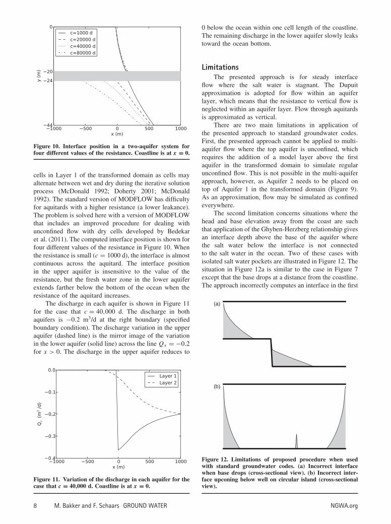
Figure 10. Interface position in a two-aquifer system forfour different values of the resistance. Coastline is at x = 0.

cells in Layer 1 of the transformed domain as cells mayalternate between wet and dry during the iterative solutionprocess (McDonald 1992; Doherty 2001; McDonald1992). The standard version of MODFLOW has difficultyfor aquitards with a higher resistance (a lower leakance).The problem is solved here with a version of MODFLOWthat includes an improved procedure for dealing withunconfined flow with dry cells developed by Bedekaret al. (2011). The computed interface position is shown forfour different values of the resistance in Figure 10. Whenthe resistance is small (c = 1000 d), the interface is almostcontinuous across the aquitard. The interface positionin the upper aquifer is insensitive to the value of theresistance, but the fresh water zone in the lower aquiferextends farther below the bottom of the ocean when theresistance of the aquitard increases.

The discharge in each aquifer is shown in Figure 11for the case that c = 40,000 d. The discharge in bothaquifers is −0.2 m3/d at the right boundary (specifiedboundary condition). The discharge variation in the upperaquifer (dashed line) is the mirror image of the variationin the lower aquifer (solid line) across the line Qx = −0.2for x > 0. The discharge in the upper aquifer reduces to

Figure 11. Variation of the discharge in each aquifer for thecase that c = 40,000 d. Coastline is at x = 0.

0 below the ocean within one cell length of the coastline.The remaining discharge in the lower aquifer slowly leakstoward the ocean bottom.

LimitationsThe presented approach is for steady interface

flow where the salt water is stagnant. The Dupuitapproximation is adopted for flow within an aquiferlayer, which means that the resistance to vertical flow isneglected within an aquifer layer. Flow through aquitardsis approximated as vertical.

There are two main limitations in application ofthe presented approach to standard groundwater codes.First, the presented approach cannot be applied to multi-aquifer flow where the top aquifer is unconfined, whichrequires the addition of a model layer above the firstaquifer in the transformed domain to simulate regularunconfined flow. This is not possible in the multi-aquiferapproach, however, as Aquifer 2 needs to be placed ontop of Aquifer 1 in the transformed domain (Figure 9).As an approximation, flow may be simulated as confinedeverywhere.

The second limitation concerns situations where thehead and base elevation away from the coast are suchthat application of the Ghyben-Herzberg relationship givesan interface depth above the base of the aquifer wherethe salt water below the interface is not connectedto the salt water in the ocean. Two of these cases withisolated salt water pockets are illustrated in Figure 12. Thesituation in Figure 12a is similar to the case in Figure 7except that the base drops at a distance from the coastline.The approach incorrectly computes an interface in the first

(a)

(b)

Figure 12. Limitations of proposed procedure when usedwith standard groundwater codes. (a) Incorrect interfacewhen base drops (cross-sectional view). (b) Incorrect inter-face upconing below well on circular island (cross-sectionalview).


section of the dropped base, where the salt water belowthe interface is not connected to the ocean. The situationin Figure 12b is equal to the situation in Figure 5, butwith a well with such a high discharge that the head atthe well is low enough that application of the Ghyben-Herzberg relationship gives an interface elevation abovethe base of the aquifer. This is not realistic, of course, asthere is no way for the salt water to reach the well.

To prevent the occurrence of these isolated pocketsof salt water, the relationship between transmissivity andhead needs to be modified such that the transmissivityis reduced only when the cell is connected to the oceanthrough other cells with a reduced transmissivity. Suchan algorithm is not currently implemented in standardgroundwater codes, but implementation seems feasible.Note that both cases in Figure 12 may be solved withthe Strack potential and will result in the correct interfacenear the coastline. A straightforward implementation ofthe Strack potential will compute similar isolated pocketsof salt water, however, unless an algorithm similar to theone discussed above is implemented.

In conclusion, isolated pockets of salt water need tobe evaluated carefully. When it is concluded that theycannot exist, a workaround may be to raise the base ofthe aquifer while simultaneously increasing the hydraulicconductivity in the area of the isolated pocket in such away that the transmissivity remains the same. Such anad-hoc approach must be applied with caution.

ConclusionsAn approach was presented to simulate steady Dupuit

interface flow in heterogeneous multi-aquifer systems withstandard single-density groundwater codes. Such casescannot be solved with codes that implement the moreelegant Strack potential, which is applicable to piecewisehomogeneous aquifers only. The approach is an efficientalternative to running transient sea water intrusion modelssuch as SEAWAT or SWI for a long time until steady stateis reached. Accuracy of the approach was demonstratedthrough comparison with exact interface flow solutions forhomogeneous aquifers obtained with Strack’s potential.An interesting next step may be to compare solutionsfor heterogeneous aquifers with results from a code thatsolves the combined flow and transport equations. Such acomparison needs to be carried out with caution, however,as deviations may be caused by a number of factors,including the vertical discretization and the (numerical)dispersion across the interface (Dausman et al. 2010).

The basic idea of the approach presented in this paperis to transform the domain such that it is identical to anunconfined flow problem. Explicit equations are given fordifferent flow types by Equations 7, 11, 22, and 25. Thevertical resistance or leakance of separating layers doesnot need to be scaled, except when the vertical resistanceor leakance is computed by the computer code, in whichcase the vertical hydraulic conductivity of the separatinglayer needs to be scaled according to Equation 30.The head and vertically integrated flow distribution are

identical in the original interface flow problem and thetransformed flow problem. Once the head is obtainedthrough the solution of the transformed flow problem,the depth of the interface may be computed from thehead with the Ghyben-Herzberg formula. Note, however,that the velocity in the real problem and the transformedmodel domain are not the same. Path line tracing cannotbe done in the transformed domain, but needs to be donein a separate model where the saturated thickness of theaquifer is set equal to the computed thickness of the freshwater zone.

Application of standard finite difference and finiteelement codes to solve for flow in the transformed domainallows for the simulation of steady interface flow in multi-aquifer systems with spatially variable aquifer properties.The codes need to be able to simulate unconfined flowwith a saturated thickness that is a linear function ofthe head, dry cells, and multi-aquifer systems whereflow in aquifers may become unconfined while there isstill flow in the aquifer directly above it. The iterativeschemes in standard groundwater codes may not always besophisticated enough to handle these nonlinear conditionsaccurately. When the standard procedures in MODFLOWfailed, the authors obtained good results using themethodology developed by Bedekar et al. (2011).

AcknowledgmentThe authors thank Vivek Bedekar for assistance with

his improved version of MODFLOW to perform thesimulations for Figures 10 and 11.

ReferencesBakker, M. 2006. Analytic solutions for interface flow in

combined confined and semi-confined, coastal aquifers.Advances in Water Resources 29, no. 3: 417–425.

Bakker, M. 2003. A Dupuit formulation for modeling seawaterintrusion in regional aquifer systems. Water ResourcesResearch 39, no. 5: 1131–1140.

Bakker, M., and F. Schaars. 2005. The Sea Water Intrusion(SWI) package manual part I. Theory, user manual, andexamples version 1.2. www.modflowswi.googlecode.com(accessed June 3, 2012).

Bakker, M., G.H.P. Oude Essink, and C.D. Langevin. 2004.The rotating movement of three immiscible fluids—abenchmark problem. Journal of Hydrology 278: 270–278.

Bear, J. 1972. Dynamics of Fluids in Porous Media. New York:Dover.

Bedekar, V., R.G. Niswonger, K. Kipp, S. Panday, andM. Tonkin. 2011. Approaches to the simulation of uncon-fined flow and perched groundwater flow in MODFLOW.Ground Water 50, no. 2: 187–198. DOI: 10.1111/j.1745-6584.2011.00829.x.

Cheng, A.H.D., D. Halhal, A. Naji, and D. Ouazar. 2000. Pump-ing optimization in saltwater-intruded coastal aquifers.Water Resources Research 36, no. 8: 2155–2165.

Dausman, A.M., C.D. Langevin, M. Bakker, and F. Schaars.2010. A comparison between SWI and SEAWAT—theimportance of dispersion, inversion and vertical anisotropy.In Proceedings of the 21st Salt Water Intrusion Meeting,June 21–26, Azores, Portugal, 2010. www.swim-site.org(accessed June 3, 2012).


Diersch, H.J.G., and O. Kolditz. 2002. Variable-density flowand transport in porous media: approaches and challenges.White Papers Vol. II. http://www.feflow.info/manuals.html(accessed June 3, 2012).

Doherty, J. 2001. Improved calculations for dewatered cells inMODFLOW. Ground Water 39, no. 6: 863–869.

Fitts, C.R. 2002. Groundwater Science. San Diego, California:Academic.

Harbaugh, A.W. 2005. MODFLOW-2005, the US GeologicalSurvey modular ground-water model—the ground-waterflow process: U.S. Geological Survey. Techniques andMethods, vol. 6-A16 (variously paginated).

Harbaugh, A.W., E.R. Banta, M.C. Hill, and M.G. McDonald.2000. MODFLOW-2000, The US Geological Survey mod-ular ground-water model—user guide to modularizationconcepts and the ground-water flow process. US GeologicalSurvey, Open-File Report 00-92.

Langevin, C.D., D.T. Thorne Jr., A.M. Dausman, M.C. Sukop,and W. Guo. 2008. SEAWAT Version 4: A ComputerProgram for Simulation of Multi-Species Solute andHeat Transport. U.S. Geological Survey. Techniques andMethods Book 6, Chapter A22, 39–p.

Mantoglou, A. 2003. Pumping management of coastal aquifersusing analytical models of saltwater intrusion. WaterResources Research 39, no. 12: 1335. DOI: 10.1029/2002WR001891.

McDonald, M.G., A.W. Harbaugh, B.R. Orr, and D.J. Ack-erman. 1992. A method of converting no-flow cells to

variable-head cells for the U.S. Geological Survey modularfinite-difference ground-water flow model. U.S. GeologicalSurvey. Open-File Report 91-536.

Pool, M., and J. Carrera. 2011. A correction factor toaccount for mixing in Ghyben-Herzberg and criticalpumping rate approximations of seawater intrusion incoastal aquifers. Water Resources Research 47, W05506.DOI: 10.1029/2010WR010256.

Post, V., H. Kooi, and C. Simmons. 2007. Using hydraulichead measurements in variable-density ground water flowanalyses. Ground Water 45, no. 6: 664–671.

Sikkema, P.C., and J.C. van Dam. 1982. Analytical formulasfor the shape of the interface in a semi-confined aquifer.Journal of Hydrology 56, no. 3–4: 201–220.

Strack, O.D.L. 1989. Groundwater Mechanics. EnglewoodCliffs, New Jersey: Prentice Hall. www.strackconsulting.com

Strack, O.D.L. 1976. A single-potential solution for regionalinterface problems in coastal aquifers. Water ResourcesResearch 12, no. 6: 1165–1174.

Voss, C.I., and A. Provost. 2010. SUTRA, a model forsaturated-unsaturated variable-density ground-water flowwith solute or energy transport. U.S. Geological SurveyWater Resources Investigation Report 02-4231, Version ofSeptember 22, 2010 (SUTRA Version 2.2).

Wooding, R.A. 1969. Growth of fingers at an unstable diffusinginterface in a porous medium or Hele-Shaw cell. Journalof Fluid Mechanics 39, no. 3: 477–495.


Documents

Modeling Steady Sea Water Intrusion with Single-Density Groundwater Codes