Embed Size (px)
Citation preview

Portland State University Portland State University
PDXScholar PDXScholar
Dissertations and Theses Dissertations and Theses
Fall 1-14-2020
Modeling Spatiotemporal Patterns of PM2.5 at the Modeling Spatiotemporal Patterns of PM2.5 at the
Sub-Neighborhood Scale Using Low-Cost Sensor Sub-Neighborhood Scale Using Low-Cost Sensor
Networks Networks
Philip Jeffrey Orlando Portland State University
Follow this and additional works at: https://pdxscholar.library.pdx.edu/open_access_etds
Part of the Environmental Sciences Commons
Let us know how access to this document benefits you.
Recommended Citation Recommended Citation Orlando, Philip Jeffrey, "Modeling Spatiotemporal Patterns of PM2.5 at the Sub-Neighborhood Scale Using Low-Cost Sensor Networks" (2020). Dissertations and Theses. Paper 5366. https://doi.org/10.15760/etd.7239
This Thesis is brought to you for free and open access. It has been accepted for inclusion in Dissertations and Theses by an authorized administrator of PDXScholar. Please contact us if we can make this document more accessible: [email protected].

Modeling Spatiotemporal Patterns of PM2.5 at the Sub-Neighborhood Scale
Using Low-Cost Sensor Networks
by
Philip Jeffrey Orlando
A thesis submitted in partial fulfillment of therequirements for the degree of
Master of Sciencein
Environmental Science and Management
Thesis Committee:Linda George, Chair
Meenakshi RaoKelly GleasonLynne Messer
Portland State University2019

i
Abstract
Epidemiological research has demonstrated an adverse relationship between
fine particulate matter (PM2.5) and human health. While PM2.5 continues to pose
a signficant global health risk, there is still the need to further characterize expo-
sures at the intra-urban scale. Land use regression is a statistical modeling tech-
nique which is used to predict air pollution concentrations at high resolution
from a limited number of monitoring sites. However, the existing regulatory
monitoring networks are typically not dense enough to apply these techniques.
We explored the potential of using low-cost PM2.5 sensor networks to overcome
the limitations of the existing regulatory monitoring infrastructure, and identi-
fied the need to determine sensor-specific correction factors based on the local
PM2.5 source profile. Once calibrated, a land use regression model (R2 = 0.89)
was developed using the low-cost sensor network (n ≈ 20), alongside several
land use and meteorological variables, to predict daily particulate matter con-
centrations at a 50 m spatial resolution during a two year period within Port-
land, Oregon. From this model, we assessed the relative strengths of expected
sources and sinks of fine particulate matter, focusing specifically on the role that
the urban canopy may play in mitigating PM2.5 exposure. This model showed
a modest but observable spatial pattern in PM2.5, but attributed the majority of
PM2.5 variation to temporal predictors (e.g. ambient background PM2.5, wind
speed, temperature). Neither proxies for traffic-related sources, or vegetation-
related sinks were identified as significant predictors of PM2.5. Our research also
demonstrated the importance of sensor placement, as a considerably different
set of predictors was selected after the inclusion of four additional monitoring

ii
sites. Future work will apply this method to four cities with a varying degree
of canopy cover to assess differences in intra-urban gradients of PM2.5 and to
further characterize the influence of vegetation.

iii
Acknowledgements
First of all, I would like to express my sincere gratitude to my advisor Dr.
Linda George for her continuous patience, guidance, and expertise throughout
my graduate study and research. I never would have imagined pursuing a grad-
uate degree without her inspiring wisdom and dedication to science.
Besides my advisor, I would like to thank the rest of my thesis committee:
Dr. Meenakshi Rao, Dr. Kelly Gleason, and Dr. Lynne Messer for their time,
encouragement, and insightful feedback.
My sincere thanks also goes to the remaining members of the Canopy Con-
tinuum project: Dr. Vivek Shandas and Dr. Todd Rosenstiel for their helpful
comments and support.
Another special thanks goes to Meenakshi Rao, as well as, Dr. Yangdong Pan
and Jackson Voelkel for cultivating my appreciation of computer science and for
teaching me how to harness it to tackle environmental problems.
I thank my fellow labmates in the Sustainable Atmospheres Research lab:
Devin Wilde, Dat Vo, Kirsten Sarle, Modi Raduma, Patrick Léon Gross, and
Kellen McInerney for their field and laboratory assistance.
I would like to thank my partner, Judit Takács, for her continual moral sup-
port and patience while I was often absorbed by my graduate work.

iv
Last but not least, I would like to thank my parents: Shannon and Jeff Or-
lando for their endless encouragement and support throughout my entire life.

v
Contents
Abstract i
Acknowledgements iii
List of Tables viii
List of Figures ix
1 Introduction 11.1 Background . . . . . . . . . . . . . . . . . . . . . . . . . . . . . . . 1
1.1.1 Particulate Matter and Human Health . . . . . . . . . . . . 11.1.2 Characterizing Particulate Matter Pollution . . . . . . . . . 21.1.3 Urban Air Quality and Traffic . . . . . . . . . . . . . . . . . 41.1.4 Influence of Vegetation on Air Quality . . . . . . . . . . . . 5
1.2 Modeling Intra-Urban PM2.5 . . . . . . . . . . . . . . . . . . . . . . 71.2.1 The Lack of Spatially Resolved PM2.5 . . . . . . . . . . . . 71.2.2 Land Use Regression Modeling of PM2.5 . . . . . . . . . . 91.2.3 Opportunities and Challenges of Low-Cost Sensors . . . . 12
1.3 Research Objectives . . . . . . . . . . . . . . . . . . . . . . . . . . . 14
2 Methodology 152.1 Low-Cost Sensor Selection . . . . . . . . . . . . . . . . . . . . . . . 15
2.1.1 Sensor Performance . . . . . . . . . . . . . . . . . . . . . . 152.1.2 PurpleAir Device Ownership and Open Data Philosophy . 17
2.2 Laboratory Evaluations . . . . . . . . . . . . . . . . . . . . . . . . . 172.3 PurpleAir Data Acquisition and Storage . . . . . . . . . . . . . . . 192.4 Opportunistic Ambient Calibration of PurpleAir Networks . . . . 212.5 Data Recovery and Sensor Lifetime . . . . . . . . . . . . . . . . . . 232.6 Sensor Allocation . . . . . . . . . . . . . . . . . . . . . . . . . . . . 232.7 Data Compilation . . . . . . . . . . . . . . . . . . . . . . . . . . . . 31
2.7.1 Spatial and Temporal Predictors of PM2.5 . . . . . . . . . . 33

vi
Road and Rail Density . . . . . . . . . . . . . . . . . . . . . 34NDVI and EVI . . . . . . . . . . . . . . . . . . . . . . . . . 34Population Density . . . . . . . . . . . . . . . . . . . . . . . 36GridMET Meteorological Variables . . . . . . . . . . . . . . 36Land Use and Land Cover . . . . . . . . . . . . . . . . . . . 37Planetary Boundary Layer Height . . . . . . . . . . . . . . 38Nephelometer PM2.5 . . . . . . . . . . . . . . . . . . . . . . 38Latitude and Longitude . . . . . . . . . . . . . . . . . . . . 39
2.7.2 Focal Statistics . . . . . . . . . . . . . . . . . . . . . . . . . . 392.7.3 Data Extraction . . . . . . . . . . . . . . . . . . . . . . . . . 41
2.8 Predictor Selection . . . . . . . . . . . . . . . . . . . . . . . . . . . 422.9 Modeling and Validation . . . . . . . . . . . . . . . . . . . . . . . . 44
3 Results and Discussion 473.1 Laboratory Evaluations . . . . . . . . . . . . . . . . . . . . . . . . . 473.2 Opportunistic Ambient Calibration . . . . . . . . . . . . . . . . . . 533.3 Predictor Selection . . . . . . . . . . . . . . . . . . . . . . . . . . . 593.4 Leave-One-Out-Cross-Validation . . . . . . . . . . . . . . . . . . . 603.5 Model Validation . . . . . . . . . . . . . . . . . . . . . . . . . . . . 623.6 Standardized Regression Coefficients . . . . . . . . . . . . . . . . . 69
3.6.1 Temporal Predictors . . . . . . . . . . . . . . . . . . . . . . 69Nephelometer PM2.5 . . . . . . . . . . . . . . . . . . . . . . 69Planetary Boundary Layer Height . . . . . . . . . . . . . . 70Season . . . . . . . . . . . . . . . . . . . . . . . . . . . . . . 70
3.6.2 Spatiotemporal Predictors . . . . . . . . . . . . . . . . . . . 71Temperature . . . . . . . . . . . . . . . . . . . . . . . . . . . 71Wind Speed . . . . . . . . . . . . . . . . . . . . . . . . . . . 72Relative Humidity . . . . . . . . . . . . . . . . . . . . . . . 72
3.6.3 Spatial Predictors . . . . . . . . . . . . . . . . . . . . . . . . 73Elevation . . . . . . . . . . . . . . . . . . . . . . . . . . . . . 73Developed Medium Intensity LULC . . . . . . . . . . . . . 73Longitude . . . . . . . . . . . . . . . . . . . . . . . . . . . . 74
3.7 Spatial Patterns of Model Residuals . . . . . . . . . . . . . . . . . 763.8 The Importance of Sensor Placement . . . . . . . . . . . . . . . . . 783.9 Predictions . . . . . . . . . . . . . . . . . . . . . . . . . . . . . . . . 83
3.9.1 Land Use Regression . . . . . . . . . . . . . . . . . . . . . . 833.9.2 Random Forest . . . . . . . . . . . . . . . . . . . . . . . . . 853.9.3 Final Model Predictions Over Time . . . . . . . . . . . . . 89
vii
4 Summary and Future Work 924.1 Summary . . . . . . . . . . . . . . . . . . . . . . . . . . . . . . . . . 924.2 Future Work . . . . . . . . . . . . . . . . . . . . . . . . . . . . . . . 94
Bibliography 97
Appendix A Source Code 117
Appendix B ThingSpeak PurpleAir Field Descriptions 346B.1 Channel A . . . . . . . . . . . . . . . . . . . . . . . . . . . . . . . . 346
B.1.1 PrimaryData . . . . . . . . . . . . . . . . . . . . . . . . . . . 346B.1.2 SecondaryData . . . . . . . . . . . . . . . . . . . . . . . . . 347
B.2 Channel B . . . . . . . . . . . . . . . . . . . . . . . . . . . . . . . . 347B.2.1 PrimaryData . . . . . . . . . . . . . . . . . . . . . . . . . . . 347B.2.2 SecondaryData . . . . . . . . . . . . . . . . . . . . . . . . . 348

viii
List of Tables
2.1 Table of Predictors . . . . . . . . . . . . . . . . . . . . . . . . . . . 46
3.1 Lab Evaluations Summary Statistics . . . . . . . . . . . . . . . . . 493.2 VIF Scores . . . . . . . . . . . . . . . . . . . . . . . . . . . . . . . . 603.3 LOOCV Summary Table . . . . . . . . . . . . . . . . . . . . . . . . 633.4 Beta Coefficients of Final Model . . . . . . . . . . . . . . . . . . . . 753.5 Beta Coefficients of Additional Model . . . . . . . . . . . . . . . . 82
ix
List of Figures
2.1 PurpleAir R2 as a Function of Distance . . . . . . . . . . . . . . . . 252.2 Albuquerque Site Map . . . . . . . . . . . . . . . . . . . . . . . . . 272.3 Boise Site Map . . . . . . . . . . . . . . . . . . . . . . . . . . . . . . 282.4 Sacramento Site Map . . . . . . . . . . . . . . . . . . . . . . . . . . 292.5 Tacoma Site Map . . . . . . . . . . . . . . . . . . . . . . . . . . . . 302.6 Workflow Diagram . . . . . . . . . . . . . . . . . . . . . . . . . . . 332.7 Focal Buffers of RLIS Streets . . . . . . . . . . . . . . . . . . . . . . 41
3.1 R2 Distributions from Lab Evaluations . . . . . . . . . . . . . . . . 493.2 Slope Distributions from Lab Evaluations . . . . . . . . . . . . . . 503.3 Scatter Plot of PurpleAir Primary Sensor and DustTrak . . . . . . 513.4 Scatter Plot of PurpleAir Secondary Sensor and DustTrak . . . . . 523.5 R2 Distributions from Field Evaluations . . . . . . . . . . . . . . . 553.6 Slope Distributions from Field Evaluations . . . . . . . . . . . . . 563.7 Scatter Plot of PurpleAir Primary Sensor and Nephelometer . . . 573.8 Scatter Plot of PurpleAir Secondary Sensor and Nephelometer . . 583.9 LOOCV Observation Bar Plot . . . . . . . . . . . . . . . . . . . . . 623.10 Scatter Plot Comparing Test Data and LUR Predictions . . . . . . 663.11 LUR Test Assumptions . . . . . . . . . . . . . . . . . . . . . . . . . 673.12 Scatter Plot Comparing Test Data and RF Predictions . . . . . . . 683.13 Map of LUR Standard Error . . . . . . . . . . . . . . . . . . . . . . 773.14 PM2.5 from both LUR Model Predictions . . . . . . . . . . . . . . . 873.15 Scatter Plot Comparing LUR Model Predictions . . . . . . . . . . 883.16 PM2.5 from both Random Forest Model Predictions . . . . . . . . 893.17 Predictions During the Wildfire Season . . . . . . . . . . . . . . . 903.18 Predictions During the Winter Season . . . . . . . . . . . . . . . . 91

1
Chapter 1
Introduction
1.1 Background
1.1.1 Particulate Matter and Human Health
Epidemiological studies have demonstrated an adverse relationship between
ambient particulate matter (PM) exposure and human health (Kloog et al., 2013;
Brunekreef and Holgate, 2002; Dockery et al., 1993). Adverse health effects
from PM exposure include cardiovascular and respiratory morbidity and mor-
tality (Le Tertre et al., 2002; Schwartz, 1994; Pope and Dockery, 2006). The
Global Burden of Disease (GBD) comparative risk assessment conducted by the
World Health Organization (WHO) attributed approximately 3.2 million year-
2010 deaths to ambient PM2.5 (PM with a diameter of 2.5 µm or smaller) expo-
sure, and ranked this pollutant as the sixth largest overall risk factor for short-
ened life expectancy globally (Lim et al., 2012; Apte et al., 2015; Fann et al.,
2012; Cohen et al., 2005). To provide further context, the global health burden
from ambient PM2.5 is greater than the cumulative health risks of other well-
established global health threats including HIV-AIDS and malaria which con-
tributed 1.5 million and 1.2 million year-2010 deaths respectively (Lim et al.,

Chapter 1. Introduction 2
2012; Apte et al., 2015). While ambient PM continues to pose a significant global
health burden, there is the need to further characterize higher granularity PM
exposure gradients, specifically at the intra-urban scale. Health studies typi-
cally rely on inter-city estimates from a limited number of monitoring sites to
develop a single exposure estimate for a given city. These single estimates are
then assigned to an entire metropolitan area, despite the potential for intra-city
heterogeneity in PM sinks and sources. This likely contributes to the underesti-
mation of PM-related health effects in the vicinity of sources (Ross et al., 2007;
Jerrett et al., 2005; Hoek et al., 2002).
1.1.2 Characterizing Particulate Matter Pollution
PM is a mixture of solid and liquid particles suspended in the air that vary in
shape, number, chemical composition and size. PM is often described by three
major size categories, the largest being coarse respirable PM, or PM10. These
are particles with a diameter less than 10 µm but greater than 2.5 µm, and are
mostly derived from biogenic or geogenic sources including the suspension or
resuspension of dust, soil, windstorms, volcanoes, pollen, mold, spores, and
sea salt. PM10 is also attributed to anthropogenic sources including agricultural
activities and mining (Pope and Dockery, 2006). Smaller than coarse PM are
fine PM, or PM2.5. These are particles that have a diameter less than or equal
to 2.5 µm. Fine PM are derived primarily from anthropogenic sources, usually
the direct result from some form of combustion. This includes vehicle emis-
sions, wood burning, coal burning, and industrial processes (steel mills, cement
plants, paper mills). In addition to primary sources of fine PM, there are also

Chapter 1. Introduction 3
secondary sources, where particles form as the result of some chemical trans-
formation in the atmosphere. Secondary fine PM is often the result of nitrogen
and sulfur oxides transforming into nitrates and sulfates, or through the for-
mation of secondary organic aerosols (SOAs) from volatile organic compound
emissions (VOCs) (Pope and Dockery, 2006). Even smaller than fine PM are
the ultrafine PM. While their definition appears to range slightly throughout
the literature, these are typically particles which have an aerodynamic diam-
eter less than 0.1 µm (Pope and Dockery, 2006; Oberdorster, Oberdorster, and
Oberdorster, 2005; EPA, 2004). Similar to fine PM, ultrafines are primarily de-
rived from some source of combustion. However, ultrafines have an extremely
short lifetime (minutes to hours), and will rapidly coagulate or condense to form
larger PM2.5 particles, which can remain suspended in the atmosphere and have
much longer residence time (days to weeks). Due to these properties, ultrafine
PM are often indicative of freshly-emitted PM from local sources.
The human health impacts from PM exposure have been shown to vary
depending on the size of the particle. Generally, the smaller the particles, the
deeper into the lungs they can infiltrate, leading to more severe health effects.
While ultrafine PM may be more capable than fine PM of transferring from the
lung to the blood and other parts of the body, there has been a focus on moni-
toring only fine and coarse PM throughout regulatory agencies due to the cost
and reproducibility of ultrafine measurements. Fine PM, in contrast to larger
particles, can remain suspended in the atmosphere for longer periods of time,
can be breathed more deeply into the lungs, and are more capable of infiltrating
indoor environments. In addition, PM10 levels throughout the US are generally

Chapter 1. Introduction 4
within compliance, whereas PM2.5 remains a regulatory challenge.
1.1.3 Urban Air Quality and Traffic
Air pollution can vary across spatiotemporal scales (Gilliland Frank et al., 2005;
Beckerman et al., 2013). Spatially, local-scale variations are the result of pri-
mary sources, whereas regional-scale variations occur from secondary reactions
and transport mechanisms. The majority of temporal variation is the result of
diurnal traffic patterns or meteorology (Beckerman et al., 2013). Generally, pol-
lutants directly emitted from mobile sources (traffic-related emissions), or in-
directly via photochemical reactions, still dominate the urban environment de-
spite significant improvements in fuel, engine, and emission control technology
over the last few decades (Fenger, 1999; Hoek et al., 2000; Nyberg et al., 2000).
It is imperative that we characterize air pollution gradients within cities as pop-
ulation density and traffic emissions are high within these environments and
exposure is not expected to be experienced evenly (Vardoulakis et al., 2003; Rao
et al., 2014). The spatial variability of primary air pollution is higher near major
intersections and busy streets within the built environment, where traffic emis-
sions are higher and ventilation is reduced due to the local topography (Har-
rison, Jones, and Barrowcliffe, 2004; Vardoulakis et al., 2003). In contrast, the
spatial variability of secondary pollutants is driven by meteorology and gen-
erally regional in scale. Many studies have identified an increase in respira-
tory and cardiovascular problems from living near major roadways (Jerrett et
al., 2008; Brugge, Durant, and Rioux, 2007; Zhou and Levy, 2007). Identifying
intra-urban pollution gradients will become increasingly relevant as rising rates

Chapter 1. Introduction 5
of urbanization and high density development result in greater human expo-
sure to near-road environments. Currently, roughly 80% of the US population
currently live within metropolitan areas (and approximately half of the global
population), and the global urban population is expected to increase to approx-
imately 68% by the year 2050 (Bureau, 2012; United Nations, 2018).
A meta-analysis conducted by Karner, Eisinger, and Niemeier, 2010 found
that many air pollutants within cities have strong pollution gradients, decaying
within 150 m - 200 m from the source, and reaching background levels between
200 m - 1000 m (Karner, Eisinger, and Niemeier, 2010). These fine-scale gradi-
ents from road sources are well documented for NO, NO2, PNC, CO, and PM10
(Karner, Eisinger, and Niemeier, 2010; Rao et al., 2014; Zhou and Levy, 2007).
However, patterns in PM2.5 mass concentration as distance from road sources
increases are less pronounced. While PM2.5 is a component of traffic-related
emissions, mass-based measurements do not always capture this influence. The
spatial patterns of PM2.5 are mixed, either decreasing very gradually from traffic
sources, or showing no clear trend at all (Karner, Eisinger, and Niemeier, 2010;
Kendrick, Koonce, and George, 2015).
1.1.4 Influence of Vegetation on Air Quality
There is an increasing body of evidence that suggests that access to greenery
can improve human health. A pioneering study conducted by Ulrich showed
that hospital patients recovering from surgery were discharged sooner and re-
quired less pain medication if they had a view of greenspace from their hos-
pital bed. This was in comparison to patients whose hospital room window

Chapter 1. Introduction 6
only provided a view of a brick wall (Ulrich, 1984). Subsequent studies have
shown that access to greenspace is associated with reduced morbidity (Maas et
al., 2009), mortality (Mitchell and Popham, 2007), and lower obesity rates (Bell,
Wilson, and Liu, 2008). In addition, recent studies have shown an association
between urban greenery (specifically trees) and air quality, suggesting that the
urban canopy has a small yet significant effect on reducing pollutants includ-
ing NO2, PM10, O3, and SO2 (Donovan et al., 2011; Rao et al., 2014; Nowak,
Crane, and Stevens, 2006). While some studies found that vegetation may only
improve the average air quality by <1-2%, this statistic accounts for multiple
pollutants, and the actual magnitude of pollution mitigation can be substantial,
typically on the order of 102 - 103 metric tons per year in a given city (Nowak,
Crane, and Stevens, 2006). Even when focusing on just a single pollutant, for
example NO2, a recent study in Portland, Oregon attributed pollution removal
by trees to providing a $7 million USD annual benefit in reduced occurrences
of respiratory complications (Rao et al., 2014). Given that trees are a fundamen-
tal component of the urban environment, with a 35% average tree cover in US
cities (Nowak and Greenfield, 2012), and that rates of urbanization are expected
to rapidly increase over the next several decades, it is crucial that we continue
to assess the potential role the urban canopy may play in reducing even more
harmful air pollutants such as PM2.5.
Trees can affect atmospheric PM concentrations by removal (Beckett, Freer-
Smith, and Taylor, 2000) and emission (e.g. pollen). Particles that physically
deposit on the leaf surface can also be resuspended, often by precipitation or
when leaves, twigs, and branches fall to the ground. While some of the particles
Chapter 1. Introduction 7
can be absorbed into the tree, most are confined to the plant surface and are ulti-
mately resuspended. As a result, trees are considered only temporary sinks for
many atmospheric particles (Nowak et al., 2013). Most of the studies related to
PM and urban trees have focused on PM10 (Nowak et al., 2013), and while some
studies have evaluated the removal rate and suspension of PM2.5 by specific
tree species (Beckett, Freer-Smith, and Taylor, 2000; Freer-Smith, El-Khatib, and
Taylor, 2004; Freer-Smith, Beckett, and Taylor, 2005; Pullman, 2008), few have
estimated the effect of trees on PM2.5 concentrations at the city-scale (Nowak
et al., 2013). There is some evidence suggesting PM2.5 mitigation by urban trees
is considerably lower relative to PM10 in terms of mass, but the health benefits
are significantly higher (Nowak, Crane, and Stevens, 2006; Nowak et al., 2013).
The benefits the urban canopy provides with PM2.5 removal is still not well un-
derstood, and only a limited number of studies have attempted to evaluate this
effect at the intra-urban scale (Nowak et al., 2013; Jeanjean, Monks, and Leigh,
2016; Tallis et al., 2011). This is due, in part, to the challenges inherent to creating
spatially resolved PM2.5 exposures surfaces at this resolution.
1.2 Modeling Intra-Urban PM2.5
1.2.1 The Lack of Spatially Resolved PM2.5
The lack of spatially resolved PM2.5 at the city-scale is mostly due to the practical
constraints of air quality monitoring networks. Due to the high cost, cumber-
some design, and the skilled labor required to establish and maintain research-
grade air quality instrumentation, the current distribution of monitoring sta-
tions is confined to a limited number of near-road and urban background sites

Chapter 1. Introduction 8
within a given city (Vardoulakis, Solazzo, and Lumbreras, 2011). For exam-
ple, within our Portland, Oregon study area, approximately 4-6 PM2.5 monitor-
ing stations were operational during the two year study period. This network,
maintained by Oregon Department of Environmental Quality (ODEQ) consisted
of a couple rural ambient background sites, urban ambient background sites,
and a single near-road site. Reference monitoring stations, typically maintained
by local or regional air quality management agencies, are primarily established
to assess regulatory compliance and develop a regional air quality index. How-
ever, the use of these monitors in epidemiological research, specifically their use
in modeling spatially resolved PM surfaces at sub-neighborhood scales (0.01 -
1.0 km), is largely an afterthought. This focus on compliance ultimately results
in the potential lack of representativeness of fixed air quality monitoring sites in
epidemiological studies. In order to account for the spatial heterogeneity of air
pollution sources in urban areas, several modeling techniques have been devel-
oped to spatially interpolate PM2.5 in order to better estimate the human health
effects from PM2.5 exposure (Vardoulakis, Solazzo, and Lumbreras, 2011). These
include land use regression (LUR) and dispersion modeling techniques (Briggs
et al., 2000; Vardoulakis, Solazzo, and Lumbreras, 2011; Hoek et al., 2008; Zhou
and Levy, 2008). For the purpose of this study, we applied LUR techniques to
develop spatially resolved PM2.5 exposures necessary for assessing the relative
power of land use sources and sinks, with a focus on the influence of vegetation.

Chapter 1. Introduction 9
1.2.2 Land Use Regression Modeling of PM2.5
Land use regression (LUR) is a statistical modeling approach which is used to
spatially predict continuous air pollution concentrations at high resolution from
a limited number of monitoring sites (Briggs et al., 2000; Rao et al., 2014). Land-
use and land-cover (LULC) variables are extracted within an appropriate buffer
distance from each monitoring location using spatial analysis software. A multi-
ple linear regression model is then developed using the monitored air pollution
data as a response variable. The model is then assessed to see how well it meets
its test assumptions. These assumptions include (1) a linear relationship exists
between the response variable and predictors, (2) model residuals are normally
distributed, (3) variation of observations around the line of best fit is constant
(homoscedasicity), (4) and strong multicollinearity among predictors is not ob-
served. This method is rooted in the principles that the environmental condi-
tions for the air pollutant response variable of interest can be determined from
a limited number of readily available predictors; and that the relationship be-
tween the response variable and predictors can be evaluated using a small sam-
ple of ’training’ data (Briggs et al., 2000). After validation, the LUR model can
be used to make spatial predictions of air pollution in between and beyond the
original monitoring network used during the training phase. Briefly, LUR mod-
els of air pollutants typically rely on predictors including population density,
land use, and traffic-related variables to characterize mean pollutant concentra-
tions within several buffer distances at specific monitoring sites. Typical buffer
sizes range between 50 m - 3000 m (Eeftens et al., 2012; Jerrett et al., 2007; Rao et
al., 2014; Liu et al., 2016). Once the model performance has been evaluated, this

Chapter 1. Introduction 10
technique can be used to make air quality predictions without the presence of a
monitoring station, essentially extrapolating pollutant exposure throughout the
remaining study area by relying on the patterns observed within the predictor
variables.
While land use regression models are capable of providing spatially resolved
air pollutant surfaces at fine scales, they still rely on observational data from a
limited number of monitoring sites for model development, calibration, and
validation (Jerrett et al., 2005; Vardoulakis, Solazzo, and Lumbreras, 2011). As a
result, the performance of LUR models depends on monitoring locations which
provide a representative sample for the remaining study area that is to be pre-
dicted. In addition, regression mapping techniques are based on assumptions
regarding their predictors, or independent variables.
Numerous LUR studies have been conducted to assess fine-scale spatially
resolved NO2 exposures because low-cost passive sampler technology has en-
abled the deployment of high-density monitoring networks (Rao et al., 2014;
Briggs et al., 2000; Eeftens et al., 2012; Hoek et al., 2008). In contrast, LUR mod-
els for particulate matter are less numerous because they necessitate a more in-
tensive monitoring campaign, despite evidence suggesting that adverse health
effects are tied more closely to PM exposure than nitrogen oxides (Eeftens et
al., 2012; Hoek et al., 2008; Pope et al., 2002; Sarnat et al., 2001). The ESCAPE
Project (European Study of Cohorts for Air Pollution Effects), a pioneering LUR
study focusing on PM2.5, produced one of the largest spatially resolved PM
databases in Europe, and relied on a total of 20 - 40 monitoring sites within
Chapter 1. Introduction 11
each of the 20 European cities examined (Eeftens et al., 2012). However, ex-
isting regulatory monitoring networks throughout our five US cities of interest
within this study are not dense enough to develop LUR models predicting intra-
urban PM2.5 (e.g. Portland n = 4, Boise n = 2, Albuquerque n = 5, Tacoma n = 2,
and Sacramento n = 7) (according to the EPA’s AirData Active PM2.5 Map) (US
EPA, 2016). Due to the aforementioned limitations of deploying high-density
networks with research-grade monitoring equipment, we opted to explore the
potential of commercially available low-cost PM2.5 sensors to achieve the rec-
ommended network density of ≥20 per city.
Previously developed LUR models of PM2.5 within the ESCAPE project have
shown moderate to good explained variance, ranging from R2 = 35%, to R2 =
94%, with a median of R2 = 71% (Eeftens et al., 2012). This range in variance
explained is partially due to limited availability of relevant GIS predictor vari-
ables across cities. As a result, no single model could be applied to each city.
Instead, area-specific predictors were selected for each city’s model due to these
differences in available predictors. Better performing models were observed to
have local traffic data available, specifically traffic intensity, and models with-
out local or limited traffic data performed below the median variance explained
(71%). Traffic variables were selected in 18 of the 20 models developed. Less im-
portant predictors included residential land use, population density, industrial
land use and ports, and natural land use (Eeftens et al., 2012). The differences
between final model R2 and Leave-One-Out Cross-Validation (LOOCV) R2 was
less than 15% for most models, indicating overall model stability (Eeftens et al.,
2012).
Chapter 1. Introduction 12
1.2.3 Opportunities and Challenges of Low-Cost Sensors
Optical Particle Counters (OPCs), also referred to as photometers, are com-
monly used for particle monitoring because of their ability to provide contin-
uous data, ease of operation, small size, and relatively low cost. This is in con-
trast to gravimetric techniques which, despite being the most accurate form of
measurement, do not provide continuous data and are costly to routinely oper-
ate and maintain. Briefly, gravimetric PM samplers actively pull an air sample
at a constant flow rate through a series of impactors to collect size-selected PM
(e.g. PM2.5 or PM10) on a filter paper over a sample period of ≥24 hours. Once
a measurable amount of PM2.5 has been collected after this sample period, the
filters are processed and weighed in a lab. The total PM2.5 mass is divided by
the total volume of air that was sampled throughout the entire sample interval
to determine a mean mass density (e.g. 10 µgm−3). This method requires a tech-
nician to routinely install and collect filters at the beginning and end of each
sample period. In contrast to collecting and weighing PM samples, OPCs rely
on a laser beam and light receptor (usually a photodiode) to measure the light
scattered from an individual illuminated aerosol particle due to Mie scattering
(Chun et al., 2001; Kim, 2004; Kohli and Mittal, 2015). The particle number
concentration (PNC) is then determined by counting the number of scattered
light pulses within a specific time interval. The particle diameter is also de-
termined by measuring the height of these light pulses. The PNC is typically
discretized into regulatory or epidemiologically relevant size bins (e.g. PM2.5,
PM10). Once discretized, PNC can be used to approximate PM mass density, but
these standalone values should be interpreted carefully. OPCs cannot be used to

Chapter 1. Introduction 13
determine aerosol type and some concessions must be made before PNC can be
converted into a mass density measurement. For example, OPCs are not able to
account for several aerosol properties, including particle density, shape, refrac-
tive index, and absorption. As a result, assumptions are made regarding each of
these properties, as OPCs report light-scattering equivalent diameters instead of
the true physical diameter and mass density (Kobayashi et al., 2014; Kohli and
Mittal, 2015). Examples of some of these assumptions include aerosol particles
having an aerodynamic diameter (particles are assumed to be spherical), with
a constant density of 1 g cm-3 (density of water), and a constant refractive in-
dex or absorption. As a result, OPCs may be more adept at approximating PM
mass of certain sources than others, which often depends on source of PM used
during the factory calibration. This information is often not disclosed by OPC
manufacturers, as the exact algorithms used to convert PNC to particle mass are
proprietary.
Despite the challenges of using OPCs to derive PM2.5 mass density, the po-
tential of these low-cost sensor networks in producing spatially resolved ex-
posure maps at finer scales relative to the existing monitoring infrastructure is
promising. If individual correction factors can be established which correspond
to the ambient PM2.5 source profile of a specific urban area, then low-cost sensor
networks may provide an advantage over traditional monitoring techniques for
LUR modeling.

Chapter 1. Introduction 14
1.3 Research Objectives
This thesis focuses on the development of (a) an opportunistic ambient calibra-
tion method for correcting low-cost PM2.5 sensor networks in order to use them
for intra-urban modeling and (b) a LUR modeling technique which relies on this
corrected sensor network data to predict spatially resolved PM2.5 throughout
Portland, Oregon in order to assess the drivers of PM2.5 intra-urban variability,
with focus on vegetation. This thesis is part of a larger epidemiological study
entitled the Canopy Continuum Project, funded by the USFS. The method de-
veloped within this thesis will be subsequently applied to four additional cities
within the USFS Canopy Continuum study (Albuquerque, New Mexico, Boise,
Idaho, Sacramento, California, and Tacoma, Washington).
The analytical goal of this study is to develop a predictive model to produce
spatially resolved PM2.5 surfaces at a spatial resolution of 50 m and a daily tem-
poral resolution throughout a 2 year period. These fine-scale exposures will be
developed for later use in an epidemiological study which characterizes the ef-
fects of several environmental stressors, including urban heat, NO2, and PM2.5
on prenatal health, and assesses the extent the urban canopy may play in help-
ing mitigate prenatal exposure to these environmental stressors.

15
Chapter 2
Methodology
2.1 Low-Cost Sensor Selection
2.1.1 Sensor Performance
We selected the PurpleAir-II SD (PurpleAir) for this study due to their pre-
viously demonstrated performance and relatively low-cost ($250). The South
Coast Air Quality Management District’s (SCAQMD) Air Quality Sensor Per-
formance Evaluation Center (AQ-SPEC) has created both lab and field evalua-
tion reports comparing several PurpleAir monitors against Federal Equivalent
Methods (FEM). They observed good correlations with FEMs during lab (R2
≈ 0.99) and field (R2 ≈ 0.95) evaluations of PM1 and PM2.5 (AQ-SPEC South
Coast AQMD, 2017b; AQ-SPEC South Coast AQMD, 2017a). AQ-SPEC also
observed moderate to good accuracy within the 0-250 µgm-3 range from the
PurpleAir monitors across multiple temperature and relative humidity profiles.
The PurpleAir monitors outperformed competing sensors that cost 2-4 times
more (MetOne E-Sampler, Alphasense OPC-N2, Dylos). The low-cost and good
accuracy of the PurpleAir monitors allowed us to installed a higher density net-
work in each of the five cities. The PurpleAir monitors are also WiFi capable,

Chapter 2. Methodology 16
and transmit data to the ThingSpeak IoT cloud platform every minute. This en-
abled the real-time monitoring of the network via a Python script which notified
us when a specific sensor lost WiFi connection or power, and data collection was
interrupted (Appendix A: purpleair_watchdog.py). We could then notify the
appropriate volunteer monitor hosts to troubleshoot the device and establish
a connection, improving long-term data recovery. The PurpleAir-II SD model
also includes local storage in the form of a micro-SD card, providing a backup if
the device loses connection to its WiFi network, or was not available at a specific
location altogether. While this appeared to be a promising feature, the current
firmware version (2.50i) of the PurpleAir-II SD had issues with data logging,
and the microcontroller would intermittently lose connection with the SD card
module. This produced data gaps and error messages were logged within the
main data file, creating further data processing issues during analysis. Upon
this discovery, we modified our sensor hosting requirements to require a WiFi
connection to avoid local storage issues.
Each PurpleAir monitor contains two Plantower PMS5003 sensors. These
are low-cost sensors ($20-$40) that approximate PM mass using an optical scat-
tering technique. The sensors record PM mass density concentrations for 1.0
µm, 2.5 µm, 5.0 µm, and 10 µm size categories using a proprietary algorithm and
come pre-calibrated from factory. The PMS5003 has additional fields that re-
port number density concentrations of particles ranging in size from 0.3 to 10.0
µm. In addition to the two Plantower PMS5003 sensors, the PurpleAir monitors
contain a Arduino ESP8266 microcontroller for wireless data communication
and logging, a BME280 pressure, temperature, and humidity sensor, an SD card

Chapter 2. Methodology 17
reader, and a real time clock to keep time while disconnected from the main
power supply. The devices also have an IP68 waterproof rating, and are de-
signed for long-term outdoor use.
2.1.2 PurpleAir Device Ownership and Open Data Philosophy
PurpleAir upholds an open data philosophy that is not matched by competing
low-cost air quality sensor manufacturers. Many sensor companies consider
data as a service, renting monitors and providing data access via monthly sub-
scription (AirAdvice, Apis Inc, MetOne, Alphasense OPC-N2, etc.). While this
may benefit the use-cases of some consumers (device troubleshooting/mainte-
nance is often included within this service), this was disadvantageous for our
research purposes. In contrast, any data collected from PurpleAir monitors is
freely available to all users, independent of device ownership. Data from third
party monitors are accessible via their application program interface (API). Af-
ter field calibration, this allowed us to incorporate data from additional third
party PurpleAir monitors into our existing network.
2.2 Laboratory Evaluations
We conducted laboratory evaluations of 65 PurpleAir monitors within a 25 °C
temperature controlled chamber at ambient humidity, and measured their re-
sponse to multiple PM sources. The low-cost PurpleAir monitors were com-
pared against a TSI DustTrak DRX 8433 Aerosol Monitor (also an optical scat-
tering instrument). PurpleAir monitors were exposed to PM generated from
smoke generated from lit matches, and smoke created by snuffing a candle
Chapter 2. Methodology 18
within the test chamber. Only one specific PM source was evaluated during
a given test. Approximately 8-10 PurpleAir monitors were suspended from the
lid of the 160L stainless steel test chamber using baling wire. The DustTrak
reference monitor was placed on the floor of the chamber to ensure adequate
ventilation between itself and the sensors hanging above. During the candle
and match smoke tests, a 100 mL beaker was placed on the floor of the cham-
ber, opposite to the sampling inlet of the DustTrak monitor. A match or candle
was lit and snuffed inside of the beaker and the chamber lid was immediately
closed. The chamber would rapidly saturate with PM well above the maximum
effective range reported by the low-cost sensor (500 µgm−3) manufacturer. The
PM would then slowly decay to zero as it was ventilated with particle-free air
(zero-air pushed through a 0.3 µm particle filter) at a constant flow-rate (inlet
pressure of 30 psi). During this time, the PM levels within the chamber were
monitored using the analog port on the DustTrak, an analog to digital convert
(A/D converter), and a Python script which provided a real-time 1-second es-
timate of the PM2.5 mass density. The entire process, from PM saturation to
below-ambient concentration, required approximately 1-2 hours per test. The
slow and steady decay of the PM within the chamber allowed us to compare
each PurpleAir monitor to the DustTrak reference across a wide range of PM
concentrations, throughout the entirety of the low-cost sensors’ effective range
(0 - 500 µgm−3). However, since we were primarily interested in sensor perfor-
mance across a environmentally relevant range, we developed individual linear
models for each sensor by comparing 1-minute averages against the reference

Chapter 2. Methodology 19
instrument between 0 - 150 µgm−3. This method allowed us to capture a near-
continuous concentration range instead of just a few discrete points that a typ-
ical span calibration would provide. Comparing the low-cost sensors across a
continuous PM range from multiple PM sources helped characterize the linear-
ity of the low-cost sensors against our reference monitor.
2.3 PurpleAir Data Acquisition and Storage
PurpleAir provides a lightweight JSON API (http://www.purpleair.com/json)
for requesting the most recent observation from each monitor, but accessing
historical data is not as straightforward. While historical data is stored by Pur-
pleAir and made available via a wagtail which requires a manual download
(http://www.purpleair.com/sensorlist), they do not provide a programmatic
interface for downloading historical data from their platform. Instead, historical
data is accessible through the ThingSpeak cloud platform. Programmatically
downloading historical data is still free and open, but it is significantly more
challenging than accessing the real-time data from the PurpleAir JSON API.
This added difficulty can be explained by two main factors. The primary fac-
tor is the API rate limit set by ThingSpeak. The size of each request is limited to a
maximum of 8000 observations. This equates to about one week’s worth of data
from a single node per request. Therefore, accessing historical data from multi-
ple devices over a long period of time (especially in the case of initial database
population) required a dynamic method of scheduling a sequence of API re-
quests based on a given start and end date. To overcome this obstacle, we de-
veloped a suite of R/Python/Bash/SQL software which dynamically identified
Chapter 2. Methodology 20
new sensors as they are installed within our study areas, and included them
into our data acquisition queue. Our system then iteratively made requests no
larger than 8000 observations across the entire lifetime of each monitor within
the network. The results from each request were then processed and stored in
our PostgreSQL database with the PostGIS extension. This preserved the spatial
coordinates associated with each PurpleAir monitor, and allowed us to perform
spatial SQL queries throughout analysis. Once our initial database was popu-
lated, a similar script was executed from a Linux server (Xubuntu 18.04) each
day at 1:00 AM using the ‘cron’ task-scheduling software. This script would up-
load the previous day’s data into the database, including any new sensors that
were installed throughout the network. It is worth noting that there are no API
rate limits in terms of request frequency (requests per unit time), and we found
success through multi-threading our pull requests. So long as each request was
no larger than 8000 observations, we could pull ThingSpeak data from every
available processor core simultaneously. This reduced our initial database pop-
ulation time by 1/8th - 1/12th depending on the available hardware (8 cores
versus 12 cores).
In addition to the API request size limit, another challenge we encountered
was the field encoding and total field limit of the PurpleAir data when stored
on the ThingSpeak platform. Relations within the ThingSpeak API are limited
to a total of eight fields, and their names are encoded (e.g. ‘field1’ instead of
‘PM1.0 (CF=ATM) ug/m3’). However, the PurpleAir monitors record 32 fields.
Therefore, requesting all of the available data from a given PurpleAir moni-
tor required four separate API requests, achieved through a combination of

Chapter 2. Methodology 21
ThingSpeak primary and secondary API keys included within the PurpleAir
JSON API. These four subsets were combined through SQL-like table joins us-
ing an R script. A key provided by PurpleAir’s technical support team was
required before these data could be fully processed (Appendix B). Once these
fields were decoded, our suite of R/Python/Bash/SQL software automated
the acquisition, processing, and storage of historical PurpleAir data (Appendix
A: purpleair_id_key.py; create_observation.sql; thingspeakCollect.R;
uploadDailyThingspeak.R; uploadHistoricalThingspeak.R).
2.4 Opportunistic Ambient Calibration of PurpleAir Networks
Since the response of each PMS5003 sensor is dependent on the PM source (in
addition to the intra-model variation observed), an opportunistic ambient cali-
bration method was developed with the goal of applying regionally-specific cor-
rection factors to each individual PMS5003 sensor within the PurpleAir network
(Portland, OR). Given that PM2.5 is not just a single pollutant, but a complex
mixture of particles from multiple primary and secondary sources, an ambient
field calibration method was required to best reflect the local PM source profile
throughout each city. To determine locally relevant correction factors for each
PMS5003 sensor in the Portland network, we compiled 5-minute nephelometer-
derived PM2.5 data provided by the Oregon Department of Environmental
Quality (ODEQ) throughout the duration of our study period (September 2017
- March 2019). Nephelometers, being an optical scattering instrument them-
selves, initially provide only a Bscat value (the extinction of light due to back

Chapter 2. Methodology 22
scattering), and are subject to the same response issues as any other optical-
based PM measurement (e.g. PurpleAir). However, a linear model was devel-
oped by ODEQ to correct these Bscat values. Nephelometers and 24 hour PM2.5
gravimetric samplers (FRM) were co-located to develop these correction fac-
tors. We used the 5-minute PM2.5 data provided by the ODEQ’s FRM-corrected
nephelometers to compare with our low-cost sensor network as a means of qual-
ity scaffolding. Depending on the day, there were 4-6 active nephelometers
throughout the entire study period. We used these nephelometers to identify pe-
riods of time where PM2.5 levels were regionally homogeneous. This consisted
of 15-minute periods (a total of three 5-minute observations per nephelometer)
where the relative standard deviation (RSD) of the ODEQ reference monitors
was less than or equal to 10%. Once windows of regionally homogeneous PM
were identified, we compared the atmospheric PM2.5 channels (‘pm2_5_atm’
as opposed to ‘pm2_5_cf_1’ which is recommended for indoor use) from both
PMS5003 sensors within a given PurpleAir monitor against the ambient back-
ground concentration (the mean of the active nephelometers) using an Ordinary
Least Squares regression (OLS) to determine sensor-specific correction factors.
These correction factors were stored as a new relation in our Postgres database
to be queried during the modeling phase. Sensors with an R2 value below 0.90
were deemed faulty or unreliable, and were excluded from the modeling phase.
This method incorporated periods of time throughout the entire study dura-
tion, allowing us to capture PM across a range of seasonal sources (wildfires,
wood heating, traffic, temperature inversions, etc.) and develop comprehensive
correction factors that account for all regionally relevant sources.

Chapter 2. Methodology 23
2.5 Data Recovery and Sensor Lifetime
Between July 2017 and December 2018 data quality issues from 7% of the
PurpleAir network were observed. While this was an improvement over the
Shinyei sensors (AirAdvice monitors) we have used during previous studies,
the PMS5003 within the PurpleAir are not immune to optical contamination
and laser diode degradation. PurpleAir’s technical support team recommended
cleaning the optics with compressed air and/or applying a vacuum to the sam-
ple inlets. Compressed air revived one out of three faulty sensors. Data re-
covery over this period was greater than 90% and the remaining network has
shown no signs of further degradation. Plantower now provides a dual-laser
model (PMS6003) which has effectively doubled the lifetime of the sensor by
alternating diodes between measurements. Modifications to the sensor chassis
and sampling path design have also demonstrated improvements to mitigating
dust accumulation in the optics in the previous models (PMS1003, PMS3003).
2.6 Sensor Allocation
The Portland, Oregon sensor network was the first in the Canopy Contin-
uum study, and PurpleAir monitors were placed opportunistically. A sensor
allocation and volunteer recruitment method was developed for the remain-
ing four cities (Albuquerque, New Mexico, Boise, Idaho, Tacoma, Washington,
and Sacramento, California). These cities were previously selected within the
Canopy Continuum project because they represent a varying degree of canopy
Chapter 2. Methodology 24
cover necessary to characterize the potential role of vegetation in mitigating en-
vironmental stressors. Our sensor allocation approach first characterized the
spatial autocorrelation of the existing Portland PurpleAir network to identify
the minimum distance necessary to capture spatially heterogeneous PM2.5. In
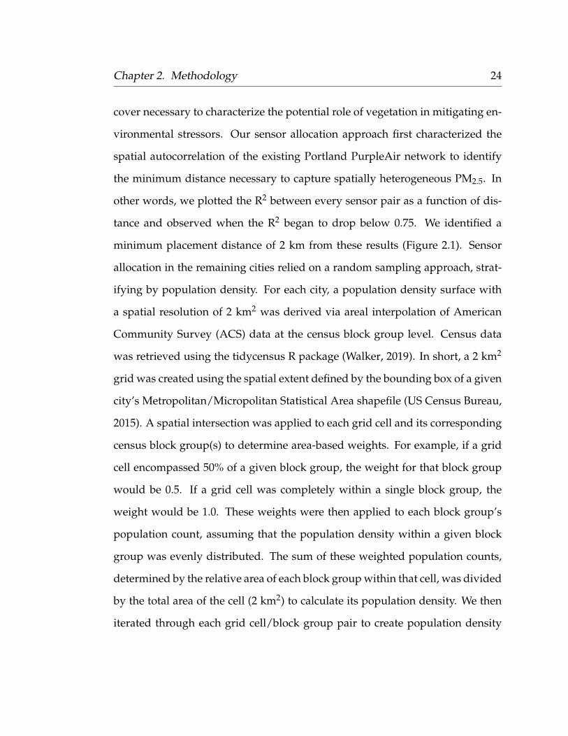
other words, we plotted the R2 between every sensor pair as a function of dis-
tance and observed when the R2 began to drop below 0.75. We identified a
minimum placement distance of 2 km from these results (Figure 2.1). Sensor
allocation in the remaining cities relied on a random sampling approach, strat-
ifying by population density. For each city, a population density surface with
a spatial resolution of 2 km2 was derived via areal interpolation of American
Community Survey (ACS) data at the census block group level. Census data
was retrieved using the tidycensus R package (Walker, 2019). In short, a 2 km2
grid was created using the spatial extent defined by the bounding box of a given
city’s Metropolitan/Micropolitan Statistical Area shapefile (US Census Bureau,
2015). A spatial intersection was applied to each grid cell and its corresponding
census block group(s) to determine area-based weights. For example, if a grid
cell encompassed 50% of a given block group, the weight for that block group
would be 0.5. If a grid cell was completely within a single block group, the
weight would be 1.0. These weights were then applied to each block group’s
population count, assuming that the population density within a given block
group was evenly distributed. The sum of these weighted population counts,
determined by the relative area of each block group within that cell, was divided
by the total area of the cell (2 km2) to calculate its population density. We then
iterated through each grid cell/block group pair to create population density
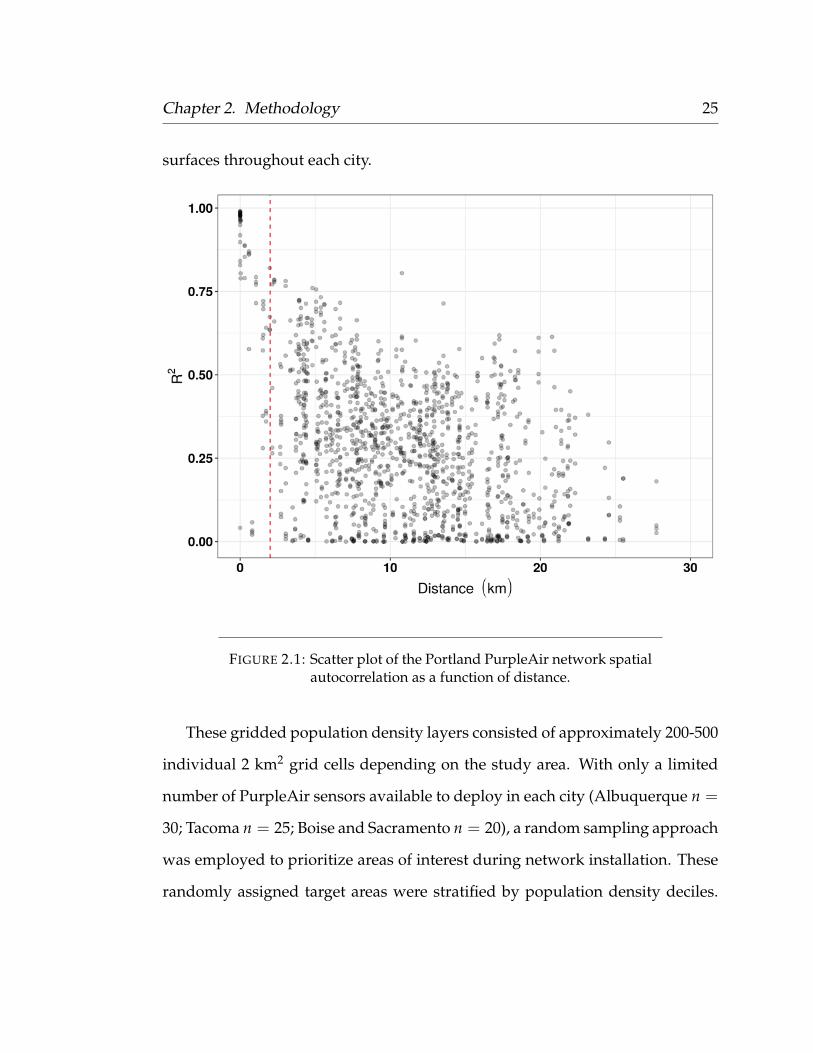
Chapter 2. Methodology 25
surfaces throughout each city.
FIGURE 2.1: Scatter plot of the Portland PurpleAir network spatialautocorrelation as a function of distance.
These gridded population density layers consisted of approximately 200-500
individual 2 km2 grid cells depending on the study area. With only a limited
number of PurpleAir sensors available to deploy in each city (Albuquerque n =
30; Tacoma n = 25; Boise and Sacramento n = 20), a random sampling approach
was employed to prioritize areas of interest during network installation. These
randomly assigned target areas were stratified by population density deciles.

Chapter 2. Methodology 26
Given that the primary goal of this study was to generate PM exposure maps for
future analysis in an epidemiological study, the majority of the target areas were
randomly assigned to the most densely populated deciles. In other words, we
attempted to recruit more volunteers to host PurpleAir monitors who lived in
more densely populated neighborhoods, and fewer volunteers from suburban
and rural neighborhoods. The total number of monitors deployed in a given city
was determined by the size of its Metropolitan Statistical Area (MSA), as well
as, the number of pre-existing 3rd party PurpleAir monitors. After the random
stratified selection process, target areas were manually adjusted for adjacency
to other target areas, as well as, any existing 3rd party PurpleAir monitors.
While this method provided a quantifiable approach to sensor allocation, the
structure of each city’s network was ultimately limited by volunteer availabil-
ity. We adopted the ‘some data is better than no data’ philosophy, and placed
the majority of our sensors wherever there were willing and able participants.
Sensors were typically installed 6-8 ft above ground in the front or backyard of
a volunteer residence. Occasionally, sensors were sited outside commercial or
government offices. This was especially the case in target areas with relatively
low population densities. Sensors were placed at least 30 ft away from hyper-
local sources including barbeques, laundry vents, and fireplaces.
Web maps with the gridded population density and sensor target areas (out-
lined in bold) were developed using leaflet R package (Cheng, Karambelkar,
and Xie, 2018). Static maps are included below and hyperlinks to the original
web maps are included within the figure captions (Figure 2.2; Figure 2.3; Figure
2.4; Figure 2.5).
Chapter 2. Methodology 27
FIGURE 2.2: Sensor allocation map developed for Albuquerque,New Mexico. Areas prioritized for sensor allocation are high-lighted in bold. The web map can be viewed here: http://web.
pdx.edu/~porlando/albuquerque.html
Chapter 2. Methodology 28
FIGURE 2.3: Sensor allocation map developed for Boise, Idaho. Ar-eas prioritized for sensor allocation are highlighted in bold. Theweb map can be viewed here: http://web.pdx.edu/~porlando/
boise.html
Chapter 2. Methodology 29
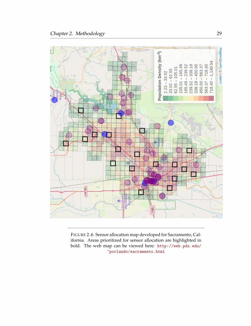
FIGURE 2.4: Sensor allocation map developed for Sacramento, Cal-ifornia. Areas prioritized for sensor allocation are highlighted inbold. The web map can be viewed here: http://web.pdx.edu/
~porlando/sacramento.html
Chapter 2. Methodology 30
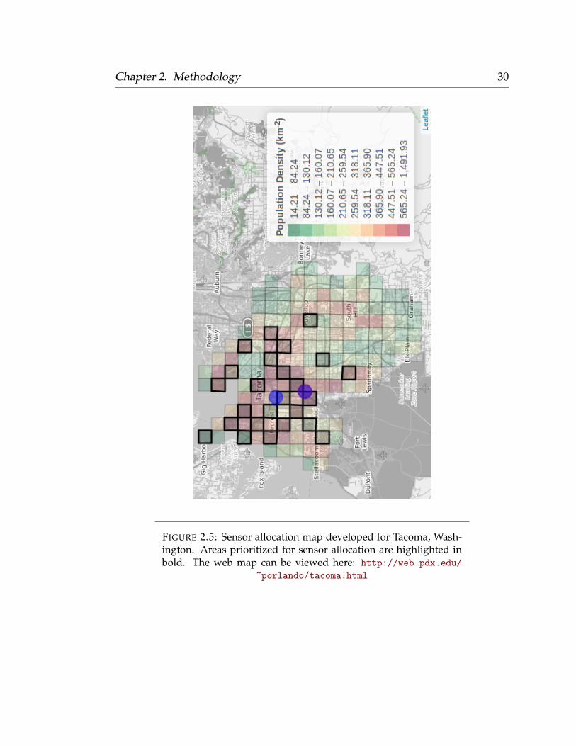
FIGURE 2.5: Sensor allocation map developed for Tacoma, Wash-ington. Areas prioritized for sensor allocation are highlighted inbold. The web map can be viewed here: http://web.pdx.edu/
~porlando/tacoma.html

Chapter 2. Methodology 31
2.7 Data Compilation
All data compilation and spatial analysis were performed using the R Statis-
tical Programming Language (R Core Team, 2019), and its corresponding spa-
tial libraries. These include ‘sp’ (Pebesma and Bivand, 2005), ‘sf’ (Pebesma,
2018), ‘raster’ (Hijmans, 2019), ‘rgdal’ (Bivand, Keitt, and Rowlingson, 2019),
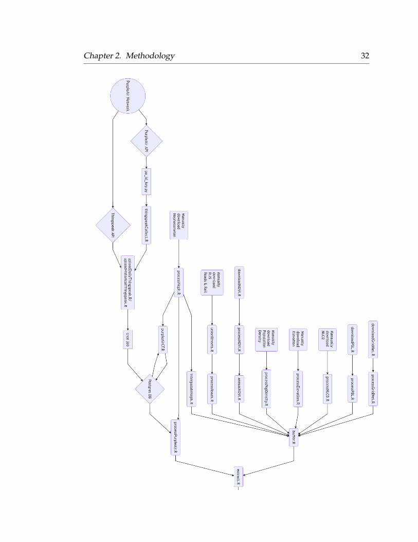
and ‘rgeos’ (Bivand and Rundel, 2019). The following workflow diagram high-
lights the various data acquisition and processing scripts necessary to develop
LUR models with corrected PurpleAir network data (Figure 2.6).
Chapter 2. Methodology 32

Chapter 2. Methodology 33
FIGURE 2.6: A workflow diagram highlighting the various datacompilation scripts necessary to develop a LUR model with cor-rected PurpleAir data. All relevant source code is included within
Appendix A.
2.7.1 Spatial and Temporal Predictors of PM2.5
Several land-use (LU) and meteorological variables were evaluated to predict
daily PM2.5 surfaces at a spatial resolution of 50 m. Land-use variables were
included as surrogates for potential PM sources in attempt to characterize the
spatial heterogeneity of PM within the study area. This included proxies of
traffic-related PM such as road (freeways, major arterials, streets, etc.) and rail
density. Other spatial predictors were included to account for potential area
sources (population density, LULC), or sinks (NDVI, EVI). Meteorological vari-
ables were included to characterize the temporal variation of PM. For example,
PM concentrations typically increase as the planetary boundary layer (PBL) de-
creases as the effective mixing volume for PM dilution decreases during low
boundary height scenarios. In addition, wind speed has been shown to affect
PM concentrations. As wind speed increases, PM generated from urban sources

Chapter 2. Methodology 34
is readily removed, diluting overall PM levels throughout the urban core (Chud-
novsky et al., 2014). The network of ODEQ PM monitors (nephelometers) were
also included as a temporal scaling factor of PM. This allowed us to capture
temporal patterns in PM that would otherwise be unaccounted for by meteoro-
logical variables alone (e.g. wildfires).
Road and Rail Density
Road and rail data were obtained from Metro’s Regional Land Information Sys-
tem (RLIS) data resource center (Oregon Metro, 2018). This included GIS shape-
files of the ‘Streets’, ‘Arterials’ ‘Major Arterials’, ‘Freeways’, ‘Railroads’, and
‘Railyards’ feature classes. Originally vector data, each feature class was dis-
cretized into a new raster layer with a spatial resolution of 50 m. These data
were also reprojected to match the Coordinate Reference System (CRS) of the
study area, and clipped by its extent (Appendix A: processRoads.R). For Port-
land, the bounding box was defined by Metro’s urban growth boundary extent
(UGB). RLIS data is not available for the other study areas, and a national-scale
data sources should be used instead during future modeling endeavors.
NDVI and EVI
Satellite-derived Normalized Difference Vegetation Index (NDVI) and En-
hanced Vegetation Index (EVI) data were obtained from the 250 m MODIS
16-day product (MOD13Q1) (Didan, 2015b).These data were programmatically
downloaded using the MODIS R package (Mattiuzzi and Detsch, 2019) (Ap-
pendix A: downloadNDVI.R). The NDVI was determined using red and near

Chapter 2. Methodology 35
infrared surface reflectances, which has been shown to provide a temporal in-
dication of vegetation cover and its phenological state (Tucker, 1979; Tucker
and Sellers, 1986). The EVI layer is more sensitive over densely vegetated ar-
eas, explaining further variation in vegetation density beyond the range of the
NDVI. Both of these layers are derived from bi-directional surface reflectances,
with masking algorithms for water, clouds (and their shadows), and aerosols
(Didan, 2015b). Each MODIS layer was reprojected to match the CRS of the
study area, clipped by the study extent, and resampled via bilinear interpola-
tion to match the 50 m spatial resolution of the model. Originally, we explored a
temporal cubic spline interpolation method to derive daily NDVI/EVI observa-
tions from each 16-day MODIS overpass (Fritsch and Carlson, 1980). While this
technique produced promising results with the 1 km resolution MODIS product
(MOD13A2), (Didan, 2015a), it did not scale to the 250 m resolution product, and
our processing script unexpectedly terminated without explanation (Appendix
A: interpolateNDVI.R). This was likely due to issues with cloud masking and
excessive missing values at this resolution. Instead of interpolating daily ND-
VI/EVI from the 250 m product, we opted to develop annual aggregates (Ap-
pendix A: annualNDVI.R).
Elevation data were retrieved from NASA’s Advanced Spaceborne Ther-
mal Emission and Reflection Radiometer (ASTER) digital elevation map (DEM)
product. This is a global DEM with a spatial resolution of 30 m provided in
GeoTiff format (NASA, 2009). This layer was reprojected to match the CRS of
our study area, clipped by our study extent, and resampled from 30 m to 50 m
(Appendix A: processElevation.R).

Chapter 2. Methodology 36
Population Density
Population density data was obtained from NASA’s Gridded Population of the
World (GPW) collection (version 4) (Doxsey-Whitfield et al., 2015). This product
models the distribution of the global human population on a continuous raster
layer for use in social, economic, and Earth science disciplines. This is a 30-arc
second resolution product (approximately 1 km) provided in GeoTIFF format.
This global raster layer was reprojected to match the CRS of our study area, and
then clipped by its extent. It was also resampled from 1 km to 50 m via bilinear
interpolation (Appendix A: processPopDensity.R).
GridMET Meteorological Variables
Meteorological data was obtained from the University of Idaho’s Gridded Sur-
face Meteorological Data (GridMET). The GridMET data is a combination of
high-resolution spatial data (4 km) from the Parameter-elevation Regressions
on Independent Slopes Model (PRISM) and the high-temporal resolution data
from the National Land Data Assimilation System (NLDAS) which generates
spatially and temporally continuous fields of several meteorological variables
(Abatzoglou, 2013; Daly, 2006; Mesinger et al., 2006). The GridMET product
provides estimates of daily precipitation totals, minimum and maximum air
temperature and relative humidity, specific humidity, mean wind direction and
mean wind speed. However, the GridMET product was not designed to capture
microclimates that occur at more granular resolutions than its native resolution
of the two parent data sources (Abatzoglou, 2013). The wind variables are lim-
ited to a 32 km spatial resolution and are not capable of capturing any influences

Chapter 2. Methodology 37
of terrain on wind fields (Abatzoglou, 2013). An R script was developed to pro-
grammatically download daily GridMET data via wget calls to a HTTP server
(Appendix A: downloadGridMET.R). As with the previous predictors, the Grid-
MET data was reprojected to match the CRS of our study area, clipped by our
study extent, and resampled to 50 m to match the resolution of our modeled sur-
faces. A bilinear interpolation was applied to all scalar variables, however, wind
direction was resampled using the nearest neighbor method because the bilin-
ear method is incapable of vector averaging (Appendix A: processGridMET.R).
Land Use and Land Cover
Land Use and Land Cover (LULC) data was obtained from the USGS’s National
Land Cover Database (NLCD) 2011 product. The NLCD provides a 30 m spatial
resolution categorical raster layer with fifteen different LULC attributes. This
includes open water, low, medium, and high intensity developed land, decid-
uous, evergreen, and mixed forest lands (Homer et al., 2015). This raster was
reprojected to match the CRS of our study area, clipped by its extent, and re-
sampled from 30 m to 50 m using the nearest neighbor method. This single
categorical layer was decomposed into individual presence/absence rasters for
each LULC attribute via one-hot encoding. For example, if the ‘open water’
LULC was observed within a raster cell, a value of 1 would be assigned to this
cell. If a LULC was not observed within a cell, then a value of 0 would be as-
signed. One-hot encoding the NLCD raster into individual layers was necessary
for creating focal statistics (Appendix A: processNLCD.R).

Chapter 2. Methodology 38
Planetary Boundary Layer Height
Planetary boundary layer height (PBL) data was obtained from NOAA’s NARR
product (Mesinger et al., 2006). An R script was used to programmatically
download 3-hourly PBL netCDF data throughout the study duration (Septem-
ber 2017 - March 2019) via wget calls to NOAA’s FTP server (Appendix A:
downloadPBL.R). The NARR PBL grid resolution is approximately 0.3 degrees,
which corresponds to 32 km at the lowest latitudes. Each 3-hourly grid was
aggregated into a single mean value throughout the study area. These 3-hour
means were then used to determine the daily maximum and minimum PBL
height values. The minimum and maximum PBL values were used as tempo-
ral scaling factors, and were extrapolated into continuous 50 m resolution spa-
tial grids corresponding to the extent and CRS of our study area (Appendix A:
processPBL.R).
Nephelometer PM2.5
Nephelometer-derived PM2.5 data with a 5-minute temporal resolution were
provided by ODEQ. In addition to the use of these data for determining cor-
rection factors for our PurpleAir sensor network, these data were also included
as a temporal scaling factor to account for changes in the ambient background
concentration due to regional sources (e.g. wildfires). The 5-minute PM2.5 val-
ues from 4-6 active nephelometers were aggregated into daily mean and median
values (Appendix A: processNeph.R). Similar to the PBL compilation, these val-
ues were extrapolated into a continuous 50 m resolution surface corresponding
to the extent and CRS of our study area (Appendix A: interpolateNeph.R).

Chapter 2. Methodology 39
Latitude and Longitude
Continuous fields for both latitude and longitude were generated using R and
its spatial libraries (raster, rgdal, rgeos, sp, sf, etc.). These variables were in-
cluded to account for the potential effects of spatial autocorrelation described
by Tobler’s 1st law of geography (Tobler, 1970).
2.7.2 Focal Statistics
Focal statistics were determined for each spatial (and temporal-spatial) pre-
dictor at 50 m, 100 m, 300 m, 500 m, and 1000 m buffer sizes (Appendix A:
buffer.R). These buffer distances were adopted from the LUR methods devel-
oped by the ESCAPE Project (Eeftens et al., 2012). The population density vari-
able also included 1250 m, 1500 m, 2000 m, and 2500 m focal buffer distances.
Briefly, this method iterates through each cell within a given 50 m resolution
spatial grid and determines the mean value of all adjacent cells within a pre-
scribed radius (neighborhood). The target cell is then assigned the mean value
of this neighborhood. This process is then repeated across the sequence of de-
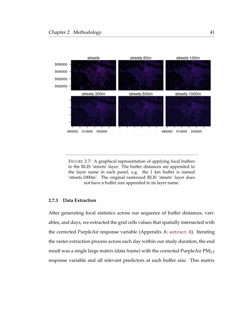
sired buffer distances. For a graphical representation of the new layers created
from applying focal statistics to the ‘Streets’ layer, see Figure 2.7. For the predic-
tors which are purely spatial (NLCD, Roads and Rail, Elevation) focal statistics
at each neighborhood size were performed only once. However, for the tem-
poral spatial-predictors (NDVI, EVI, GridMET), this operation was repeated for
each daily observation. This resulted in a total of 33 thousand individual raster
layers, stored as GeoTIFFs, which consumed approximately 100 GB of local disk

Chapter 2. Methodology 40
storage. Despite being rasterized, this method was also computationally expen-
sive. Determining thousands of focal buffers required the use of a high-memory
compute server provided by PSU Research Computing, and consumed geq500
GB of memory while running on all 24 available processor cores. Processing
time was on the order of 4-6 hours depending on the total number of predictors
selected for modeling.
The temporal predictors lacking any spatial component (e.g. scaling factors
including PBL and Nephelometer PM) were not included in the focal statistics
pipeline, as these layers only consisted of a single mean value for each day.
Focal statistics for the GridMET wind direction data were handled differ-
ently than the other variables. This layer, with the inclusion of wind speed, was
converted from degrees to radians, and then transposed into its respective u
(zonal velocity) and v (meridional velocity) components. Focal statistics were
then performed on the u and v components (unit-vector averaging), and con-
verting back into degrees using the arc-tangent (Appendix A: buffer.R).
Chapter 2. Methodology 41
FIGURE 2.7: A graphical representation of applying focal buffersto the RLIS ‘streets’ layer. The buffer distances are appended tothe layer name in each panel, e.g. the 1 km buffer is named‘streets.1000m’. The original rasterized RLIS ‘streets’ layer does
not have a buffer size appended to its layer name.
2.7.3 Data Extraction
After generating focal statistics across our sequence of buffer distances, vari-
ables, and days, we extracted the grid cells values that spatially intersected with
the corrected PurpleAir response variable (Appendix A: extract.R). Iterating
the raster extraction process across each day within our study duration, the end
result was a single large matrix (data frame) with the corrected PurpleAir PM2.5
response variable and all relevant predictors at each buffer size. This matrix

Chapter 2. Methodology 42
consisted of 211 variables and 11,546 observations. Additional categorical vari-
ables were added to this matrix including ‘Weekday/Weekend’, ‘Day of Week’,
‘Season’, and ‘Month’. This matrix was used during the modeling phase. The
study duration consisted of 575 consecutive days and, given the 11,546 unique
observations, the average number of active PurpleAir monitors on a given day
was approximately 20. This is comparable to the network sizes within the ES-
CAPE Project (Eeftens et al., 2012). The Portland network did grow overtime
as PurpleAir monitors were incrementally added by our research group as well
as other 3rd parties. The network size was closer to 10 active nodes during the
first few months of the study, and grew to more than 35 nodes by its end. Some
of these were active for a short period of time, but most remained active once
initially established.
2.8 Predictor Selection
To avoid issues of multicollinearity, only a single focal buffer distance was se-
lected for each predictor variable during the modeling phase. A correlation
matrix was produced for each variable against the response data and the fo-
cal buffer with the strongest correlation with the response variable was then
selected for modeling. If multiple focal buffers had the same correlation coef-
ficient, then the finest spatial resolution buffer was chosen to capture as much
spatial heterogeneity as possible. Variables with nonintuitive correlations, e.g.
expected sources yielding a negative correlation, or expected sinks yielding a
positive correlation, were excluded from the model.

Chapter 2. Methodology 43
An additional correlation matrix which compared all of the previously se-
lected predictors was generated to explore groups which covaried. A complete
linkage hierarchical clustering algorithm, a built-in parameter within the R ‘cor-
rplot’ library (Wei and Simko, 2017), was used to identify clustered predictors
(Defays, 1977). Once these groups were identified, only a single predictor within
each group was selected for the modeling phase. For example, if the NLCD-
derived ‘Deciduous Forest’, ‘Mixed Forest’, ‘Evergreen Forest’ were clustered
with ‘NDVI’, then the most generalizeable predictor was selected for the final
model (e.g. the NDVI layer can be used to explain all of the other vegetation
layers).
These predictor selection criteria were established to meet the multi-
collinearity assumption of a traditional multiple linear regression. We relied
on a Variance Inflation Factor (VIF) below 5 to meet this assumption. VIF scores
were determined using the ‘car’ R library to assess multicollinearity (Fox et al.,
2007). Although the multicollinearity assumption only applies to multiple lin-
ear regression model, the same variable selection procedure was applied to the
Random Forest model for direct comparison. Model variables were also tested
for significance, and only predictor coefficient’s p-value less than 0.1 were se-
lected for the final model (Appendix A: modeling.R).
The initial predictors selected for the modeling phase are included within
Table 2.1. This table details the variable description, abbreviation, and respec-
tive data sources. The expected source and sink proxies for each predictor are
also included.
Chapter 2. Methodology 44
2.9 Modeling and Validation
For this study, we compared the performance of a traditional LUR model (mul-
tiple linear regression) against a decision-tree-based machine learning model
(Random Forest) (Liaw and Wiener, 2002; Breiman, 2001). Of the 11,546 to-
tal observations, we randomly subset 70% during the training phase for each
model. The remaining 30%, or ’test’ data, was reserved for model validation.
In addition to this 70/30 holdout approach, we also employed a leave-one-
out cross-validation (LOOCV) method which has been widely used in previous
LUR studies (Yang et al., 2017; Eeftens et al., 2012; Saucy et al., 2018). With this
approach, a single PurpleAir node was excluded from the training data and a
model was developed using the n − 1 remaining sites. The subsequent model
was then used to predict all of the observations for this single node, and the
model performance was evaluated by observing the cross validation (CV) R2
and CV RMSE. This process was then repeated for each individual node, ex-
cluding nodes with fewer than 100 observations. The LOOCV method allowed
us to evaluate how well a given model predicted for a specific sensor over a
consecutive period of time, instead of predicting a random subset of days and
sensors simultaneously. In addition, this method allowed us to compare an en-
tire ensemble of predictions (a new model was developed for each node that was
left out), and identify any locations that a model was consistently under/over
predicting.
An ensemble method was used during the LUR model prediction phase.
Specifically, each of the n − 1 models developed during the LOOCV phase were

Chapter 2. Methodology 45
used to predict an individual PM2.5 surface. This ensemble of predictions was
then aggregated to determine a single mean PM2.5 surface each day. The Ran-
dom Forest method was too computationally expensive to rely on the LOOCV
technique when making predictions. Instead, the results from the single model
which included all available monitoring sites generated from the 70/30 holdout
process was used during the prediction phase.
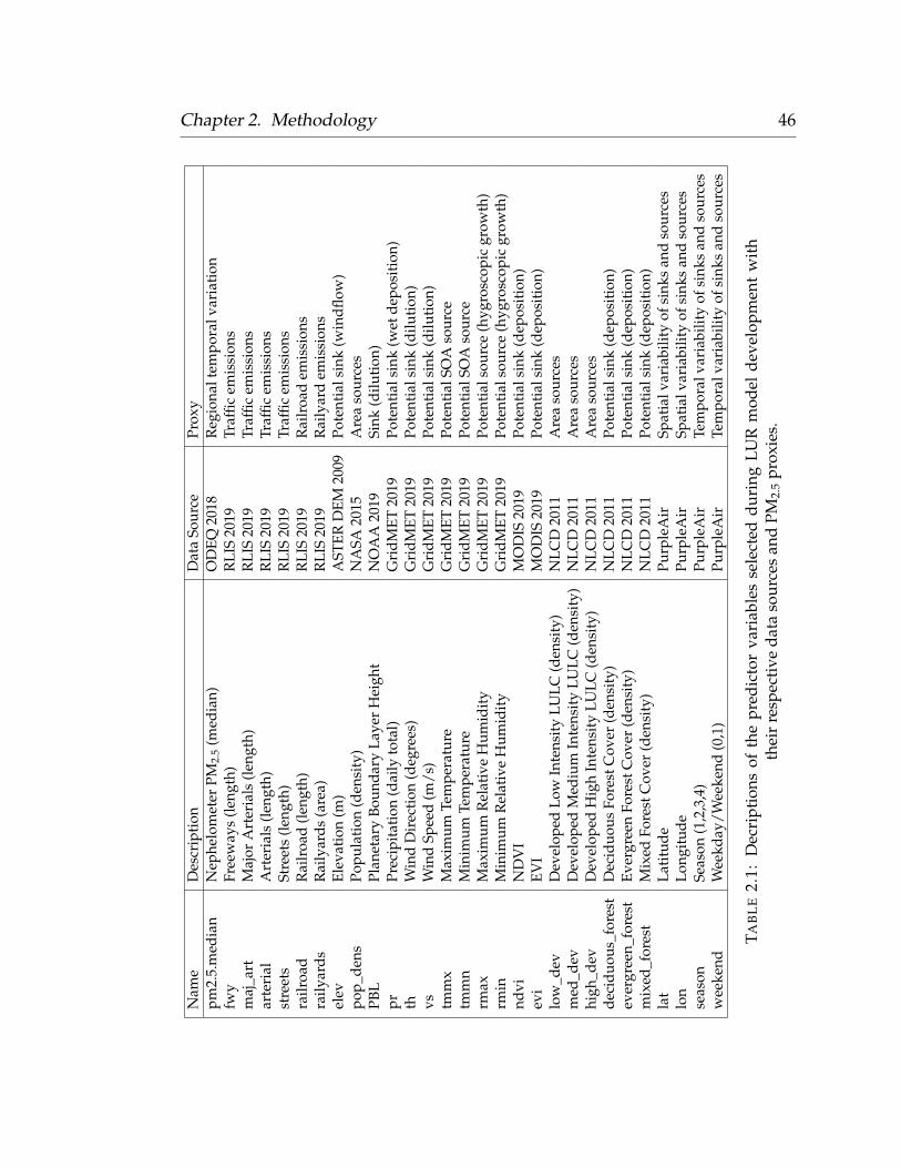
Chapter 2. Methodology 46
Nam
eD
escr
ipti
onD
ata
Sour
cePr
oxy
pm2.
5.m
edia
nN
ephe
lom
eter
PM2.
5(m
edia
n)O
DEQ
2018
Reg
iona
ltem
pora
lvar
iati
onfw
yFr
eew
ays
(len
gth)
RLI
S20
19Tr
affic
emis
sion
sm
aj_a
rtM
ajor
Art
eria
ls(l
engt
h)R
LIS
2019
Traf
ficem
issi
ons
arte
rial
Art
eria
ls(l
engt
h)R
LIS
2019
Traf
ficem
issi
ons
stre
ets
Stre
ets
(len
gth)
RLI
S20
19Tr
affic
emis
sion
sra
ilroa
dR
ailr
oad
(len
gth)
RLI
S20
19R
ailr
oad
emis
sion
sra
ilyar
dsR
aily
ards
(are
a)R
LIS
2019
Rai
lyar
dem
issi
ons
elev
Elev
atio
n(m
)A
STER
DEM
2009
Pote
ntia
lsin
k(w
indfl
ow)
pop_
dens
Popu
lati
on(d
ensi
ty)
NA
SA20
15A
rea
sour
ces
PBL
Plan
etar
yBo
unda
ryLa
yer
Hei
ght
NO
AA
2019
Sink
(dilu
tion
)pr
Prec
ipit
atio
n(d
aily
tota
l)G
ridM
ET20
19Po
tent
ials
ink
(wet
depo
siti
on)
thW
ind
Dir
ecti
on(d
egre
es)
Gri
dMET
2019
Pote
ntia
lsin
k(d
iluti
on)
vsW
ind
Spee
d(m
/s)
Gri
dMET
2019
Pote
ntia
lsin
k(d
iluti
on)
tmm
xM
axim
umTe
mpe
ratu
reG
ridM
ET20
19Po
tent
ialS
OA
sour
cetm
mn
Min
imum
Tem
pera
ture
Gri
dMET
2019
Pote
ntia
lSO
Aso
urce
rmax
Max
imum
Rel
ativ
eH
umid
ity
Gri
dMET
2019
Pote
ntia
lsou
rce
(hyg
rosc
opic
grow
th)
rmin
Min
imum
Rel
ativ
eH
umid
ity
Gri
dMET
2019
Pote
ntia
lsou
rce
(hyg
rosc
opic
grow
th)
ndvi
ND
VI
MO
DIS
2019
Pote
ntia
lsin
k(d
epos
itio
n)ev
iEV
IM
OD
IS20
19Po
tent
ials
ink
(dep
osit
ion)
low
_dev
Dev
elop
edLo
wIn
tens
ity
LULC
(den
sity
)N
LCD
2011
Are
aso
urce
sm
ed_d
evD
evel
oped
Med
ium
Inte
nsit
yLU
LC(d
ensi
ty)
NLC
D20
11A
rea
sour
ces
high
_dev
Dev
elop
edH
igh
Inte
nsit
yLU
LC(d
ensi
ty)
NLC
D20
11A
rea
sour
ces
deci
duou
s_fo
rest
Dec
iduo
usFo
rest
Cov
er(d
ensi
ty)
NLC
D20
11Po
tent
ials
ink
(dep
osit
ion)
ever
gree
n_fo
rest
Ever
gree
nFo
rest
Cov
er(d
ensi
ty)
NLC
D20
11Po
tent
ials
ink
(dep
osit
ion)
mix
ed_f
ores
tM
ixed
Fore
stC
over
(den
sity
)N
LCD
2011
Pote
ntia
lsin
k(d
epos
itio
n)la
tLa
titu
dePu
rple
Air
Spat
ialv
aria
bilit
yof
sink
san
dso
urce
slo
nLo
ngit
ude
Purp
leA
irSp
atia
lvar
iabi
lity
ofsi
nks
and
sour
ces
seas
onSe
ason
(1,2
,3,4
)Pu
rple
Air
Tem
pora
lvar
iabi
lity
ofsi
nks
and
sour
ces
wee
kend
Wee
kday
/Wee
kend
(0,1
)Pu
rple
Air
Tem
pora
lvar
iabi
lity
ofsi
nks
and
sour
ces
TAB
LE
2.1:
Dec
ript
ions
ofth
epr
edic
tor
vari
able
sse
lect
eddu
ring
LUR
mod
elde
velo
pmen
tw
ith
thei
rre
spec
tive
data
sour
ces
and
PM2.
5pr
oxie
s.
47
Chapter 3
Results and Discussion
3.1 Laboratory Evaluations
Strong linear relationships between the low-cost PurpleAir monitors and the
reference DustTrak DRX Aerosol Monitor Model 8533 were observed for both
the match and candle smoke tests. The mean R2 of the candle smoke evalua-
tions was 0.958 ± 0.14, whereas the mean R2 of the match smoke evaluations
was 0.942 ± 0.17 Table 3.1. Despite following the same protocol between tests,
some sensors did not perform linearly with the reference instrument (Figure
3.1). However, these cases occurred infrequently and meaningful calibrations
with R2 values greater than 0.90 occurred for more than 80% of all test peri-
ods. While the strength of DustTrak-PurpleAir relationship was independent
of the PM source, the slopes differed depending on the PM source. The mean
slope of the models generated from the match smoke tests was 1.35 ± 0.64. This
was approximately half the value observed from the candle smoke tests which
yielded a mean slope of 2.66 ± 0.75 (Figure 3.2). These results indicate two
challenges with low-cost PM sensors for LUR. The first was that intra-model
Chapter 3. Results and Discussion 48
variation does occur with the Plantower sensors, despite the manufacturer’s ef-
fort to pre-calibrate each sensor. This means that two sensors, when exposed
to the same PM sample, will produce a slightly different response. The slopes
from the match smoke tests are more narrowly distributed, while the candle
smoke tests have a wider distribution ranging from 2-3 and appear bimodal.
This was somewhat unexpected because multiple different types of matches
were used throughout these laboratory evaluations, whereas only a single can-
dle was used. This could potentially be explained by match smoke PM having
similar physical properties as Plantower’s PM source during factory calibra-
tion (e.g. absorption, profile, shape, etc.). The second challenge presented by
these results is that the Plantower/PurpleAir response is dependent on the PM
source. This suggests that laboratory calibrations alone, while a reliable screen-
ing tool for faulty sensors, are not enough to determine meaningful correction
factors for field-deployed sensors necessary to produce epidemiologically rel-
evant PM2.5 concentrations. These results support the development of an am-
bient calibration method of PurpleAir networks for determining field-specific
correction factors. Two scatter plots were included to highlight the PurpleAir’s
response across the entire PM range of a typical test for both the primary and
secondary sensors (A and B sensors) (Figure 3.3; Figure 3.4).
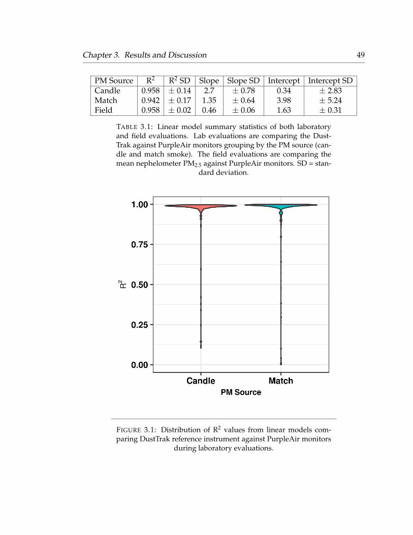
Chapter 3. Results and Discussion 49
PM Source R2 R2 SD Slope Slope SD Intercept Intercept SDCandle 0.958 ± 0.14 2.7 ± 0.78 0.34 ± 2.83Match 0.942 ± 0.17 1.35 ± 0.64 3.98 ± 5.24Field 0.958 ± 0.02 0.46 ± 0.06 1.63 ± 0.31
TABLE 3.1: Linear model summary statistics of both laboratoryand field evaluations. Lab evaluations are comparing the Dust-Trak against PurpleAir monitors grouping by the PM source (can-dle and match smoke). The field evaluations are comparing themean nephelometer PM2.5 against PurpleAir monitors. SD = stan-
dard deviation.
FIGURE 3.1: Distribution of R2 values from linear models com-paring DustTrak reference instrument against PurpleAir monitors
during laboratory evaluations.
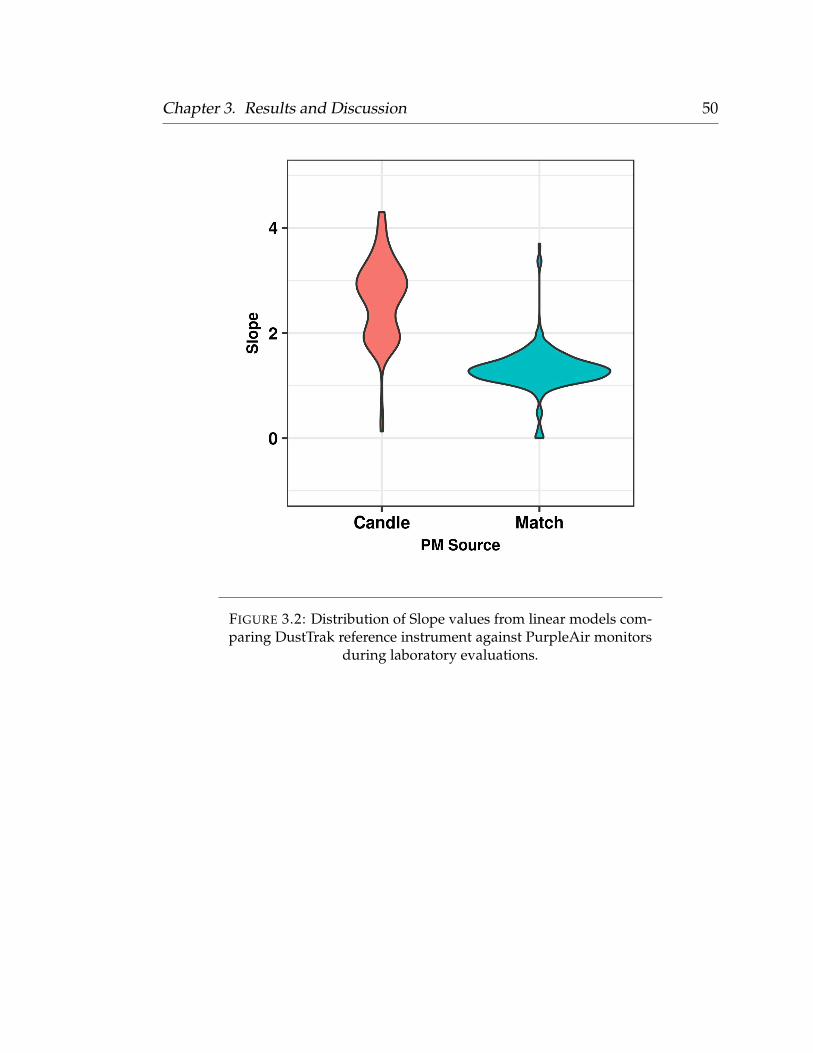
Chapter 3. Results and Discussion 50
FIGURE 3.2: Distribution of Slope values from linear models com-paring DustTrak reference instrument against PurpleAir monitors
during laboratory evaluations.
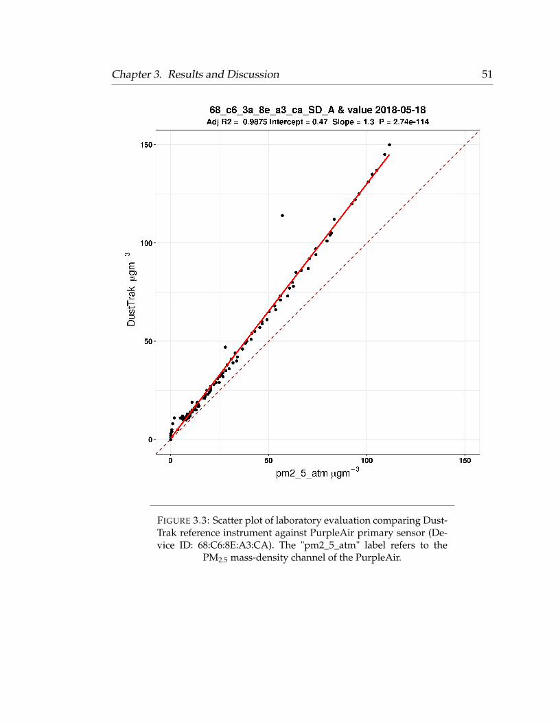
Chapter 3. Results and Discussion 51
FIGURE 3.3: Scatter plot of laboratory evaluation comparing Dust-Trak reference instrument against PurpleAir primary sensor (De-vice ID: 68:C6:8E:A3:CA). The "pm2_5_atm" label refers to the
PM2.5 mass-density channel of the PurpleAir.
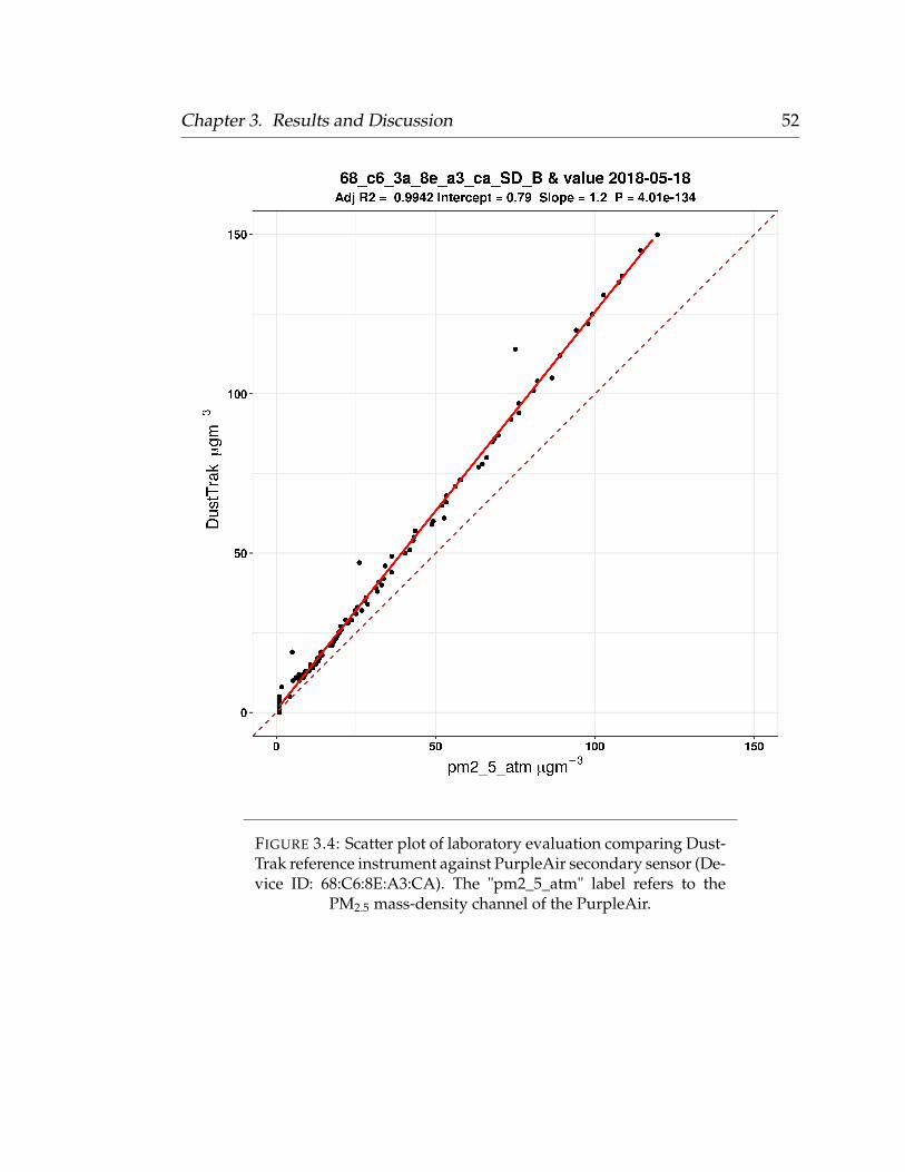
Chapter 3. Results and Discussion 52
FIGURE 3.4: Scatter plot of laboratory evaluation comparing Dust-Trak reference instrument against PurpleAir secondary sensor (De-vice ID: 68:C6:8E:A3:CA). The "pm2_5_atm" label refers to the
PM2.5 mass-density channel of the PurpleAir.

Chapter 3. Results and Discussion 53
3.2 Opportunistic Ambient Calibration
Based on the laboratory calibration findings, we sought a way to calibrate sen-
sors in-situ with ambient particulate matter. Based on other studies (Eeftens et
al., 2012; Zhou and Levy, 2007), PM2.5 levels can be mainly driven by regional
sources thereby limiting small-scale variability. We tested the idea of calibrating
the sensors during regional homogeneity events. Homogeneity was assessed
using the 4-6 ODEQ nephelometers in the Portland metro area. These neph-
elometers have been calibrated against the federal reference method. Originally
5-minute resolution data, the nephelometers were aggregated to 15-minute
means to identify periods when PM2.5 was determined to be regionally homo-
geneous (the relative standard deviation of all active nephelometers within the
Portland metropolitan area was ≤ 10%). Once these periods were identified,
linear models were generated for each sensor, and those with an R2 < 0.90, or
those with < 100 observations were excluded from the modeling phase (Ap-
pendix A: homogeneousPM.R). Violin plots were created to graphically assess the
distribution of R2 and slope values during the field calibrations. The R2 values
from the field evaluations were not as narrowly distributed below 1.0 relative
to the laboratory evaluations, and considerable left-skew of the R2 distribution
was observed. This suggests that the some sensors were affected by local PM
sources that were otherwise not captured by the network of nephelometers. Fig-
ure 3.5 shows the distribution of R2 for the 138 sensors with the nephelometers
during homogeneity events. We chose an R2 of 0.90 as our quality filter. Af-
ter applying the quality filter to the 138 unique sensors observed throughout
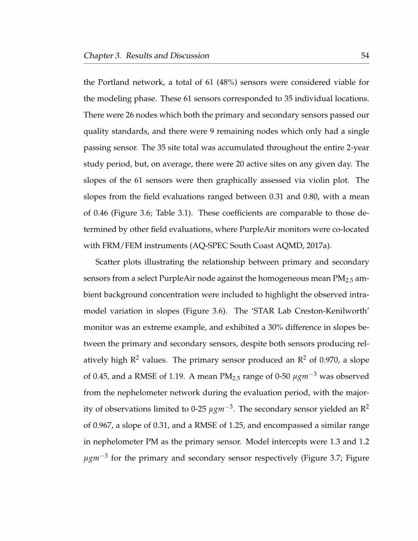
Chapter 3. Results and Discussion 54
the Portland network, a total of 61 (48%) sensors were considered viable for
the modeling phase. These 61 sensors corresponded to 35 individual locations.
There were 26 nodes which both the primary and secondary sensors passed our
quality standards, and there were 9 remaining nodes which only had a single
passing sensor. The 35 site total was accumulated throughout the entire 2-year
study period, but, on average, there were 20 active sites on any given day. The
slopes of the 61 sensors were then graphically assessed via violin plot. The
slopes from the field evaluations ranged between 0.31 and 0.80, with a mean
of 0.46 (Figure 3.6; Table 3.1). These coefficients are comparable to those de-
termined by other field evaluations, where PurpleAir monitors were co-located
with FRM/FEM instruments (AQ-SPEC South Coast AQMD, 2017a).
Scatter plots illustrating the relationship between primary and secondary
sensors from a select PurpleAir node against the homogeneous mean PM2.5 am-
bient background concentration were included to highlight the observed intra-
model variation in slopes (Figure 3.6). The ‘STAR Lab Creston-Kenilworth’
monitor was an extreme example, and exhibited a 30% difference in slopes be-
tween the primary and secondary sensors, despite both sensors producing rel-
atively high R2 values. The primary sensor produced an R2 of 0.970, a slope
of 0.45, and a RMSE of 1.19. A mean PM2.5 range of 0-50 µgm−3 was observed
from the nephelometer network during the evaluation period, with the major-
ity of observations limited to 0-25 µgm−3. The secondary sensor yielded an R2
of 0.967, a slope of 0.31, and a RMSE of 1.25, and encompassed a similar range
in nephelometer PM as the primary sensor. Model intercepts were 1.3 and 1.2
µgm−3 for the primary and secondary sensor respectively (Figure 3.7; Figure
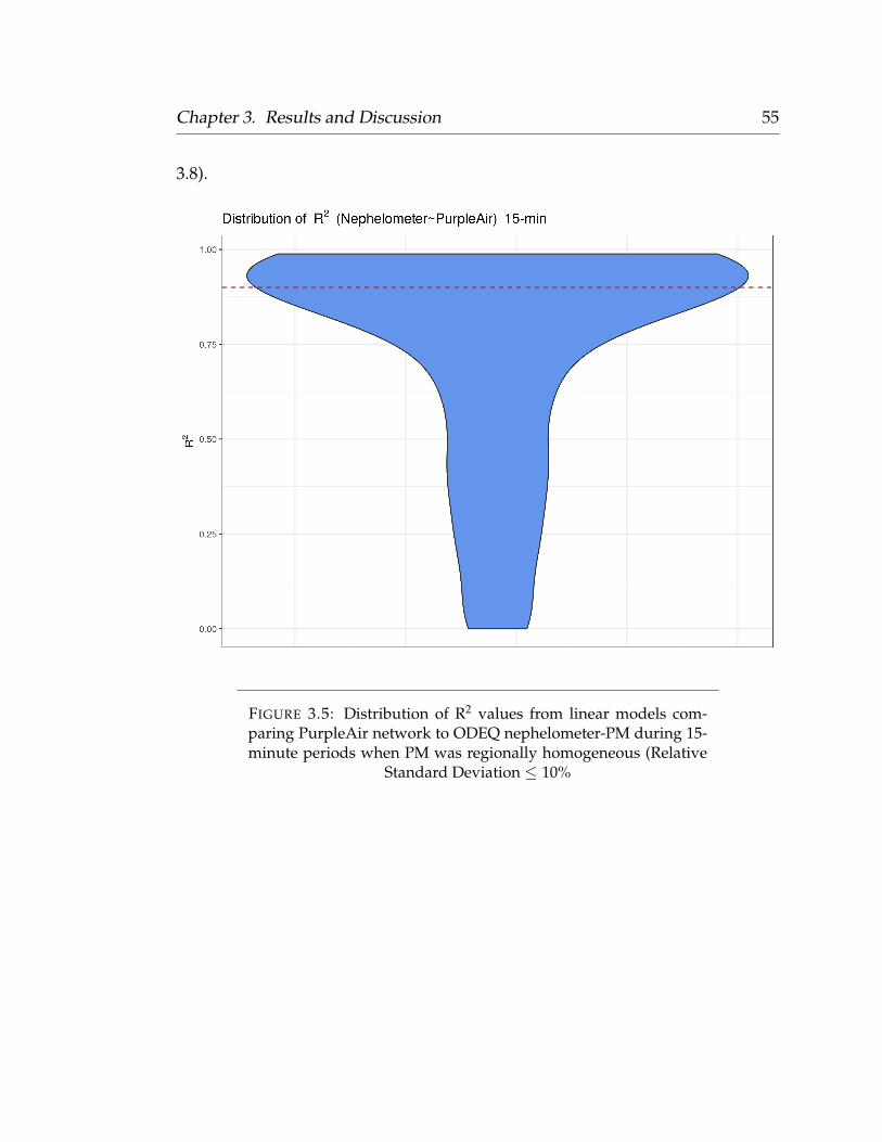
Chapter 3. Results and Discussion 55
3.8).
FIGURE 3.5: Distribution of R2 values from linear models com-paring PurpleAir network to ODEQ nephelometer-PM during 15-minute periods when PM was regionally homogeneous (Relative
Standard Deviation ≤ 10%
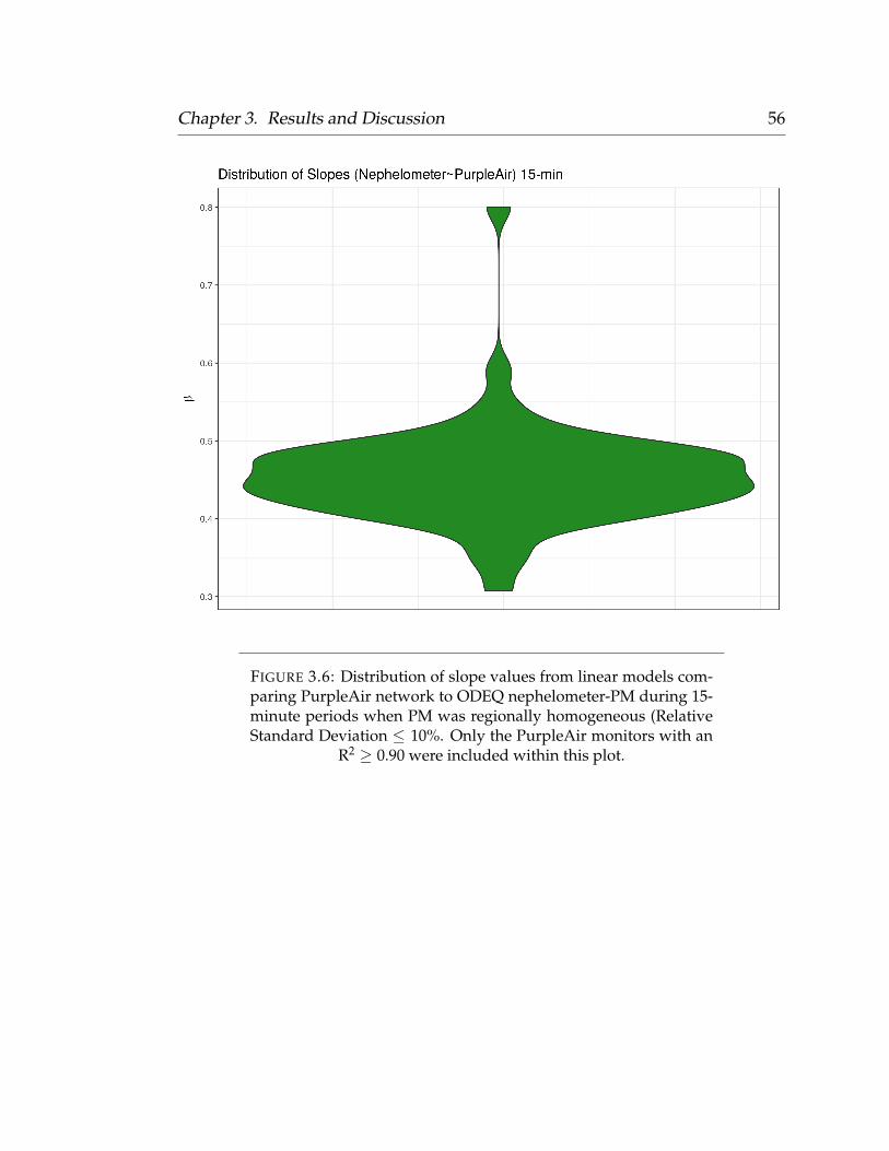
Chapter 3. Results and Discussion 56
FIGURE 3.6: Distribution of slope values from linear models com-paring PurpleAir network to ODEQ nephelometer-PM during 15-minute periods when PM was regionally homogeneous (RelativeStandard Deviation ≤ 10%. Only the PurpleAir monitors with an
R2 ≥ 0.90 were included within this plot.
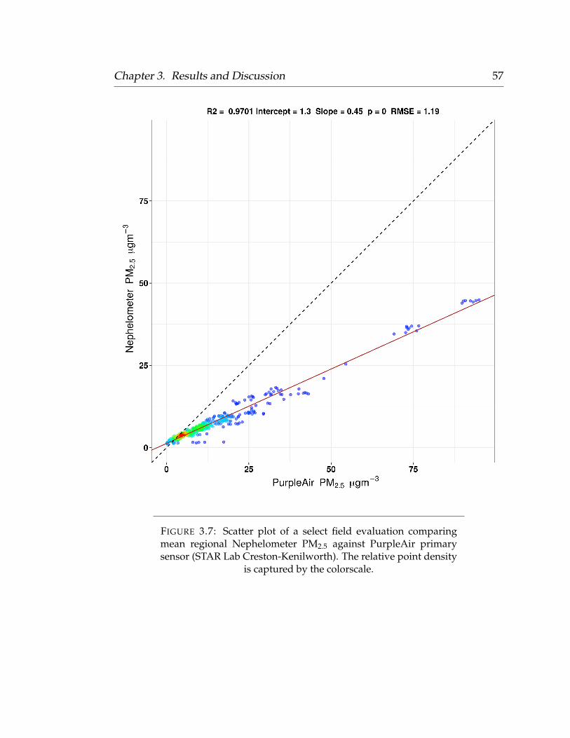
Chapter 3. Results and Discussion 57
FIGURE 3.7: Scatter plot of a select field evaluation comparingmean regional Nephelometer PM2.5 against PurpleAir primarysensor (STAR Lab Creston-Kenilworth). The relative point density
is captured by the colorscale.
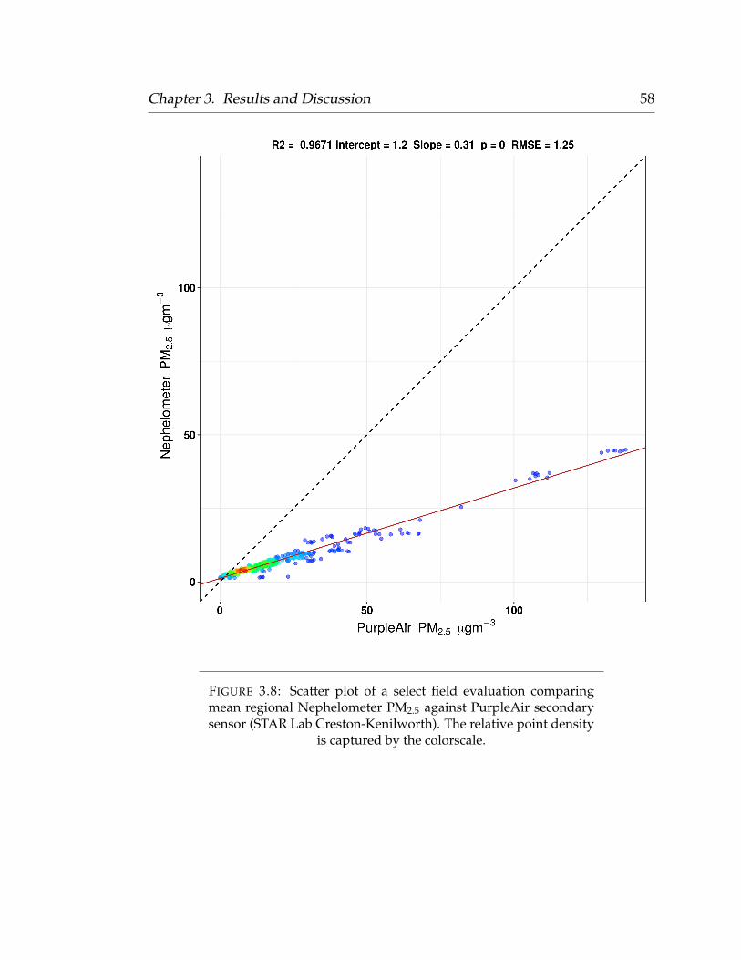
Chapter 3. Results and Discussion 58
FIGURE 3.8: Scatter plot of a select field evaluation comparingmean regional Nephelometer PM2.5 against PurpleAir secondarysensor (STAR Lab Creston-Kenilworth). The relative point density
is captured by the colorscale.

Chapter 3. Results and Discussion 59
3.3 Predictor Selection
The goal of the modeling effort is to predict PM2.5 at high spatial resolution and
identify the land-use or physical drivers of variability. The next step for model
development was to identify variables for the inclusion in the model. Purpose-
ful variable selection was performed partly by software and partly by hand. We
relied on previous literature and our understanding of the physical properties
of PM2.5 to derive our set of proxies for expected sources and sinks (Eeftens et
al., 2012; Rao et al., 2014; Brokamp et al., 2017; Saucy et al., 2018; Wang and
Ogawa, 2015; Chudnovsky et al., 2014). A list of all initial predictors that were
considered are outlined in Table 2.1. Only a single buffer for each spatial predic-
tor was selected for the subsequent modeling phases to avoid issues regarding
multicollinearity. We then narrowed down our selected predictors by explor-
ing clusters which covaried. Finally, a stepwise Akaike Information Criterion
(AIC) reduction method was employed to further narrow the set of predictors
into a final parsimonious model, referred to as the ‘final model’. We relied on
the hybrid selection method, which is a combination of both forward and back-
ward selection techniques (Venables and Ripley, 2002). Of the 28 predictors ini-
tially considered, only 9 were included within our final explanatory model. It
is worth noting that the spatial and spatiotemporal variables each had multi-
ple buffer distances, and the total number of initial predictors was considerably
higher than 28 prior to the selection of a single buffer per variable. The 9 final
predictors were selected based on correlation strength with the response vari-
able, VIF scores below 5, intuitive signs of model coefficients (i.e. potential sinks
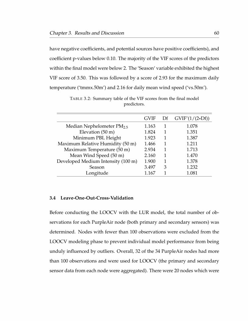
Chapter 3. Results and Discussion 60
have negative coefficients, and potential sources have positive coefficients), and
coefficient p-values below 0.10. The majority of the VIF scores of the predictors
within the final model were below 2. The ‘Season‘ variable exhibited the highest
VIF score of 3.50. This was followed by a score of 2.93 for the maximum daily
temperature (‘tmmx.50m’) and 2.16 for daily mean wind speed (‘vs.50m’).
TABLE 3.2: Summary table of the VIF scores from the final modelpredictors.
GVIF Df GVIFˆ(1/(2*Df))
Median Nephelometer PM2.5 1.163 1 1.078Elevation (50 m) 1.824 1 1.351
Minimum PBL Height 1.923 1 1.387Maximum Relative Humidity (50 m) 1.466 1 1.211
Maximum Temperature (50 m) 2.934 1 1.713Mean Wind Speed (50 m) 2.160 1 1.470
Developed Medium Intensity (100 m) 1.900 1 1.378Season 3.497 3 1.232
Longitude 1.167 1 1.081
3.4 Leave-One-Out-Cross-Validation
Before conducting the LOOCV with the LUR model, the total number of ob-
servations for each PurpleAir node (both primary and secondary sensors) was
determined. Nodes with fewer than 100 observations were excluded from the
LOOCV modeling phase to prevent individual model performance from being
unduly influenced by outliers. Overall, 32 of the 34 PurpleAir nodes had more
than 100 observations and were used for LOOCV (the primary and secondary
sensor data from each node were aggregated). There were 20 nodes which were
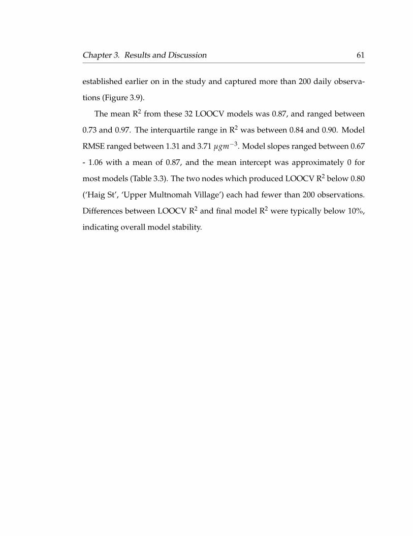
Chapter 3. Results and Discussion 61
established earlier on in the study and captured more than 200 daily observa-
tions (Figure 3.9).
The mean R2 from these 32 LOOCV models was 0.87, and ranged between
0.73 and 0.97. The interquartile range in R2 was between 0.84 and 0.90. Model
RMSE ranged between 1.31 and 3.71 µgm−3. Model slopes ranged between 0.67
- 1.06 with a mean of 0.87, and the mean intercept was approximately 0 for
most models (Table 3.3). The two nodes which produced LOOCV R2 below 0.80
(‘Haig St’, ‘Upper Multnomah Village’) each had fewer than 200 observations.
Differences between LOOCV R2 and final model R2 were typically below 10%,
indicating overall model stability.
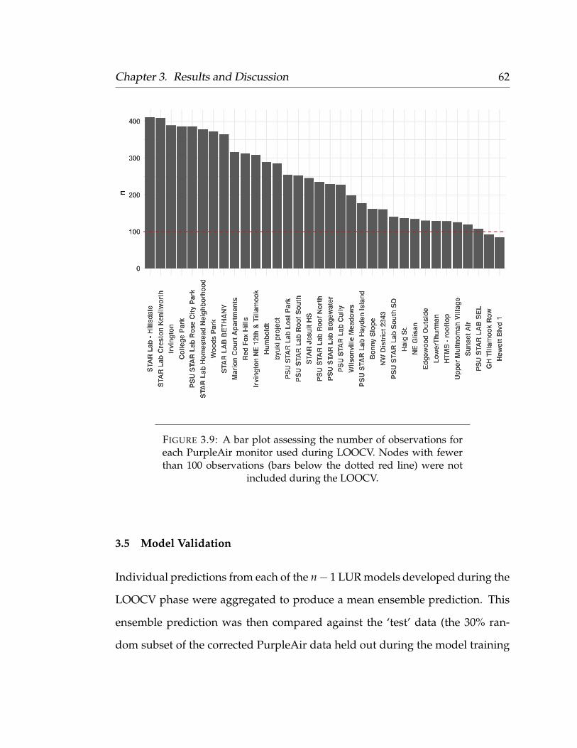
Chapter 3. Results and Discussion 62
FIGURE 3.9: A bar plot assessing the number of observations foreach PurpleAir monitor used during LOOCV. Nodes with fewerthan 100 observations (bars below the dotted red line) were not
included during the LOOCV.
3.5 Model Validation
Individual predictions from each of the n− 1 LUR models developed during the
LOOCV phase were aggregated to produce a mean ensemble prediction. This
ensemble prediction was then compared against the ‘test’ data (the 30% ran-
dom subset of the corrected PurpleAir data held out during the model training
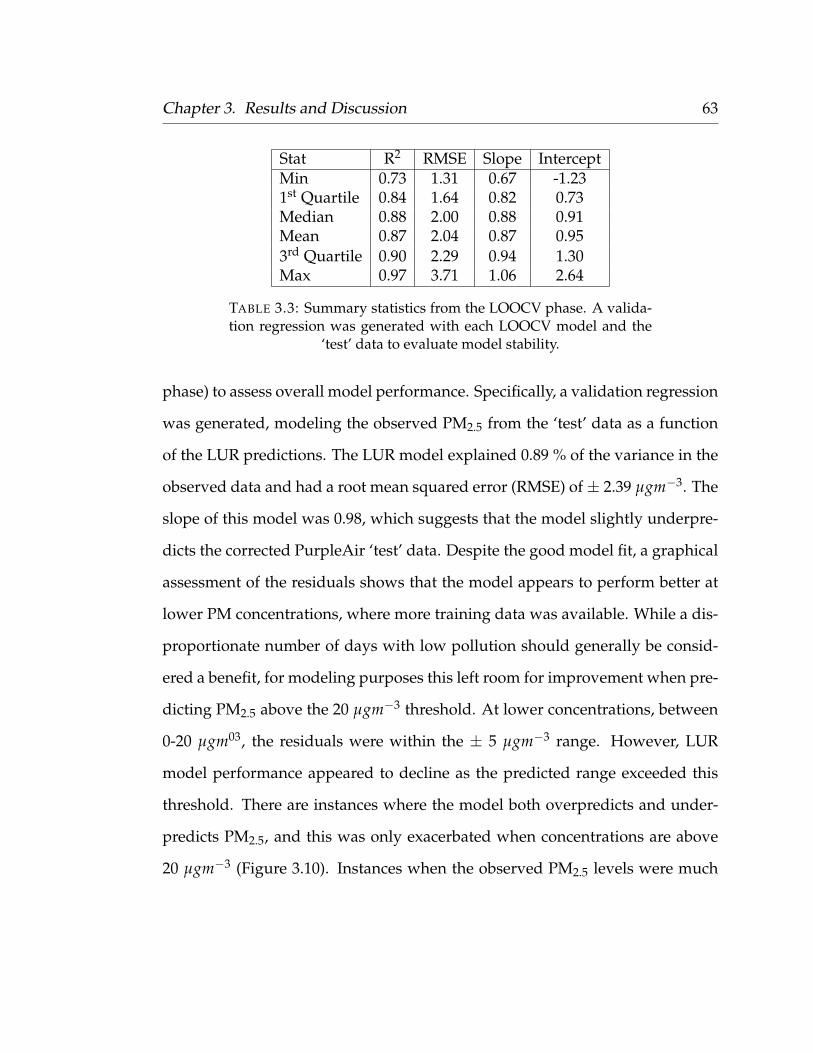
Chapter 3. Results and Discussion 63
Stat R2 RMSE Slope InterceptMin 0.73 1.31 0.67 -1.231st Quartile 0.84 1.64 0.82 0.73Median 0.88 2.00 0.88 0.91Mean 0.87 2.04 0.87 0.953rd Quartile 0.90 2.29 0.94 1.30Max 0.97 3.71 1.06 2.64
TABLE 3.3: Summary statistics from the LOOCV phase. A valida-tion regression was generated with each LOOCV model and the
‘test’ data to evaluate model stability.
phase) to assess overall model performance. Specifically, a validation regression
was generated, modeling the observed PM2.5 from the ‘test’ data as a function
of the LUR predictions. The LUR model explained 0.89 % of the variance in the
observed data and had a root mean squared error (RMSE) of ± 2.39 µgm−3. The
slope of this model was 0.98, which suggests that the model slightly underpre-
dicts the corrected PurpleAir ‘test’ data. Despite the good model fit, a graphical
assessment of the residuals shows that the model appears to perform better at
lower PM concentrations, where more training data was available. While a dis-
proportionate number of days with low pollution should generally be consid-
ered a benefit, for modeling purposes this left room for improvement when pre-
dicting PM2.5 above the 20 µgm−3 threshold. At lower concentrations, between
0-20 µgm03, the residuals were within the ± 5 µgm−3 range. However, LUR
model performance appeared to decline as the predicted range exceeded this
threshold. There are instances where the model both overpredicts and under-
predicts PM2.5, and this was only exacerbated when concentrations are above
20 µgm−3 (Figure 3.10). Instances when the observed PM2.5 levels were much

Chapter 3. Results and Discussion 64
higher than the predicted levels suggest days when the regional monitoring net-
work was unable to capture some local PM source at a given PurpleAir node.
The test assumptions of the LUR model were graphically assessed and can
be viewed in Figure 3.11. The ‘Residuals vs Fitted’ panel shows the red trendline
appears to approximate the zero line, which indicates that the linearity assump-
tion is being met. The ‘Normal Q-Q’ panel shows that the residuals are nor-
mally distributed between the -2 and 2 theoretical quantiles, but the normality
assumption is not met across the entire range of model residuals. The ‘Scale-
Location’ panel shows the red trendline increasing as the fitted values increase.
This means that the LUR model does not meet the homoscedascity assumption.
However, since we were mostly interested in our ability to predict PM2.5 concen-
trations that typically occur within the urban environment (0 - 20 µgm−3), we
were willing to move forward with the model prediction phase, acknowledg-
ing that the spatial variability of exceptionally high PM events (e.g. forest fires)
must be interpreted with caution. Finally, the ‘Residuals vs Leverage’ panel is
used to evaluate potenitally influential outliers that located beyond Cook’s dis-
tance. Despite our lack of normally distributed residuals, no data points were
observed to exceed this distance.
In addition to the LUR model, we explored using a random forest (RF)
model for its expectedly higher predictive power and its ability to account for
some of the limitations inherent to LUR. Land use regression models have diffi-
culty capturing non-linear relationships and complex interactions, but random
forests (RF) are resistant to these problems. Random forests are often preferred
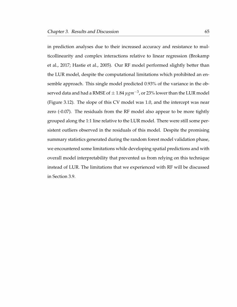
Chapter 3. Results and Discussion 65
in prediction analyses due to their increased accuracy and resistance to mul-
ticollinearity and complex interactions relative to linear regression (Brokamp
et al., 2017; Hastie et al., 2005). Our RF model performed slightly better than
the LUR model, despite the computational limitations which prohibited an en-
semble approach. This single model predicted 0.93% of the variance in the ob-
served data and had a RMSE of ± 1.84 µgm−3, or 23% lower than the LUR model
(Figure 3.12). The slope of this CV model was 1.0, and the intercept was near
zero (-0.07). The residuals from the RF model also appear to be more tightly
grouped along the 1:1 line relative to the LUR model. There were still some per-
sistent outliers observed in the residuals of this model. Despite the promising
summary statistics generated during the random forest model validation phase,
we encountered some limitations while developing spatial predictions and with
overall model interpretability that prevented us from relying on this technique
instead of LUR. The limitations that we experienced with RF will be discussed
in Section 3.9.
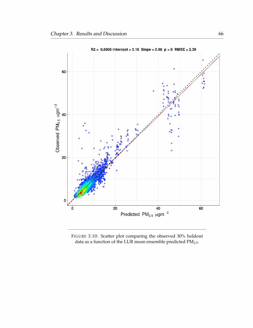
Chapter 3. Results and Discussion 66
FIGURE 3.10: Scatter plot comparing the observed 30% holdoutdata as a function of the LUR mean ensemble predicted PM2.5.
Chapter 3. Results and Discussion 67
FIGURE 3.11: A graphical assessement of the LUR model’s abilityto meet multiple linear regression test assumptions.
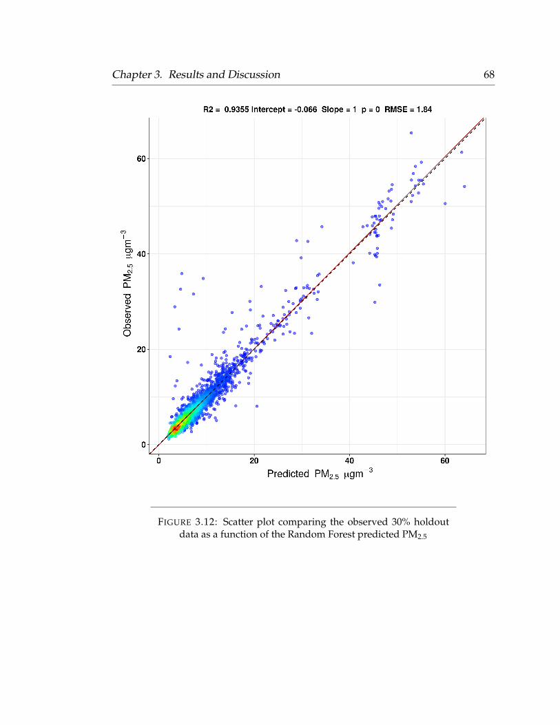
Chapter 3. Results and Discussion 68
FIGURE 3.12: Scatter plot comparing the observed 30% holdoutdata as a function of the Random Forest predicted PM2.5

Chapter 3. Results and Discussion 69
3.6 Standardized Regression Coefficients
3.6.1 Temporal Predictors
Nephelometer PM2.5
The final model included the median PM2.5 of the nephelometer network
(the ODEQ regional monitoring network), elevation, the minimum planetary
boundary layer height, the maximum relative humidity and temperature, mean
wind speed, developed medium intensity LULC, season, and longitude. The
standardized regression coefficients (betas) of the final LUR model show that
the median nephelometer PM2.5 value (‘pm2.5.median’) had the strongest asso-
ciation with PM2.5 concentrations observed from the PurpleAir network. A one
standard deviation increase in median nephelometer PM2.5 corresponded to a
0.908 increase in standard deviation of the PurpleAir network. The unstandard-
ized coefficient for the median nephelometer PM2.5 indicates a 0.834 increase in
PurpleAir PM2.5 for every 1.0 µgm−3 increase in the ambient background con-
centration. The daily median nephelometer PM2.5 concentration can be inter-
preted as a temporal scaling factor, and the variation in the PurpleAir network
can largely be explained simply by the variation in the ambient background con-
centration. This was not surprising, as Karner et al. previously identified little
to no spatial variation with intra-urban PM2.5 (Karner, Eisinger, and Niemeier,
2010). Instead, meteorology mostly drives the temporal variation, while the
spatial variability of this pollutant typically occurs at regional scales (Table 3.4).
The association of the remaining 8 predictors and PM2.5 was much weaker, each
with beta values below 0.10.
Chapter 3. Results and Discussion 70
Planetary Boundary Layer Height
The minimum planetary boundary layer height (‘pbl.min’) was shown to have
the 7th highest beta value. An increase in one standard deviation in minimum
PBL height resulted in a 0.015 decrease in the standard deviation of our re-
sponse network. This variable corresponds to the minimum atmospheric vol-
ume available for dilution of urban sources. PBL was primarily included to cap-
ture days when meteorological conditions were stable, and temperature inver-
sions were expected to trap surface-emitted PM2.5, resulting in elevated concen-
trations during the cold season (Table 3.4). It was surprising that this variable
did not have as strong an association with PM2.5 as some of the other temporal
predictors (e.g. wind speed and maximum daily temperature).
Season
A categorical ‘Season’ variable was included to account for recurring seasonal
patterns in PM2.5 variation over the 2 year study period. While the the fall sea-
son had the fourth highest beta coefficient in the final model, the other two
seasons (spring and summer) had some of the lowest associations with the Pur-
pleAir response network (Table 3.4).
Another categorical variable was considered during the initial predictor se-
lection phase to account for patterns in human activity (traffic, area sources)
on weekends versus weekdays. This variable was also included to account for
the lack of traffic intensity data that has been widely used throughout previ-
ous LUR studies. Weekdays were expected to have higher PM2.5 levels due to
increase traffic intensity during the work week commute relative to weekends.
Chapter 3. Results and Discussion 71
However, this variable was not determined to be significant during the LUR
model development.
3.6.2 Spatiotemporal Predictors
Temperature
The daily maximum temperature at a 50 m resolution had the second highest
beta value. A one standard deviation increase in maximum daily temperature
at 50 m (‘tmmx.50m’) resulted in a 0.073 decrease in standard deviation of the
PM2.5 levels from our response network. Several potential proxies were con-
sidered with the inclusion of temperature data in the final LUR model. On the
one hand, higher temperatures correspond with a larger mixing volume, pro-
viding a surrogate for increased dilution. However, on the other hand, higher
temperatures also enable higher rates of secondary organic aerosol formation,
potentially leading to higher PM2.5 levels in our response network (Wang and
Ogawa, 2015). Additionally, higher temperatures are also associated with the
wild fire season within the Portland, Oregon, and some of the most polluted
days observed within the training data occurred during the warm season. De-
spite the uncertainties regarding which proxy would potentially drive the asso-
ciation between temperature and PM2.5, we chose to include ‘tmmx.50m’ in the
final LUR model due to its coefficient’s significance. Here, we can interpret this
negative beta coefficient to be due to the influence from wildfires, and perhaps
slightly by SOA formation. It is worth noting that although temperature was
the second most important predictor its beta was only 8% of the nephelometer-
derived PM2.5 beta (Table 3.4). In other words, the majority of the variation in

Chapter 3. Results and Discussion 72
our PurpleAir data was explained by the ambient background concentration of
the nephelometers.
Wind Speed
Wind speed was identified to be somewhat associated with PM2.5, and had the
3rd highest beta coefficient. This predictor was included as a surrogate for dilu-
tion, as PM2.5 from local sources are readily removed from the urban environ-
ment was wind speeds increase. As this predictor increased by one standard
deviation, the response variable was observed to decrease by 0.063 standard de-
viations (Table 3.4). During data compilation, wind direction was determined to
be too coarse of a spatial resolution and was excluded from the modeling phase.
Relative Humidity
The maximum relative humidity at 50 m (‘rmax’) was shown to be one of the
least associated predictors with the PurpleAir PM2.5. An increase of one stan-
dard deviation of this variable was associated with only a 0.011 decrease in the
response network. Similar to the maximum temperature layer, relative humid-
ity was included to account for multiple potential affects on PM2.5 concentra-
tions. Generally, when relative humidity increases, PM2.5 mass density is ob-
served to also increase due to hygroscopic growth. However, after a certain
relative humidity threshold, PM2.5 levels have been observed to decline as hy-
groscopic growth produces particles which are too large to remain suspended in
Chapter 3. Results and Discussion 73
the air, ultimately depositing (Wang and Ogawa, 2015). Despite these uncertain-
ties, this variable was included within the final LUR model due to its significant
p-value (Table 3.4).
3.6.3 Spatial Predictors
Elevation
Elevation at a 50 m resolution (‘elev.50m’) was shown to be the most influential
spatial predictor within the final LUR model. Most of the spatial variation ob-
served in the model predictions approximated this elevation layer. This predic-
tor had the 5th highest beta value, and an increase by one standard deviation in
elevation resulted in a 0.03 decrease in standard deviation of our response net-
work. This variable was a proxy for dilution, as wind speeds are typically higher
at higher elevations and less shielded by surface roughness. The inclusion of
this variable was an effort to capture some of the finer-scale topographical ef-
fects on PM2.5 that were unaccounted for by the GridMET wind speed product.
The majority of primary urban PM2.5 is emitted near the surface, and can be-
come trapped at lower elevations during stable meteorological conditions.
Developed Medium Intensity LULC
The developed medium intensity LULC variable at the 100 m buffer size
(‘med_dev’ or ‘developed_medium_intensity.100m’) was shown to have the 6th
highest beta. A one standard deviation increase in medium developed LULC
corresponded to a 0.023 increase in standard deviation of the response network.
In other words, the more medium developed LULC observed within 100 m of
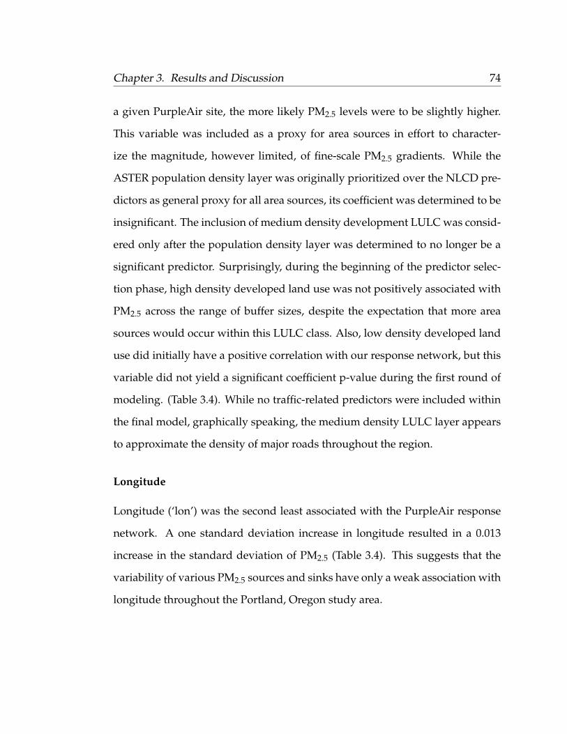
Chapter 3. Results and Discussion 74
a given PurpleAir site, the more likely PM2.5 levels were to be slightly higher.
This variable was included as a proxy for area sources in effort to character-
ize the magnitude, however limited, of fine-scale PM2.5 gradients. While the
ASTER population density layer was originally prioritized over the NLCD pre-
dictors as general proxy for all area sources, its coefficient was determined to be
insignificant. The inclusion of medium density development LULC was consid-
ered only after the population density layer was determined to no longer be a
significant predictor. Surprisingly, during the beginning of the predictor selec-
tion phase, high density developed land use was not positively associated with
PM2.5 across the range of buffer sizes, despite the expectation that more area
sources would occur within this LULC class. Also, low density developed land
use did initially have a positive correlation with our response network, but this
variable did not yield a significant coefficient p-value during the first round of
modeling. (Table 3.4). While no traffic-related predictors were included within
the final model, graphically speaking, the medium density LULC layer appears
to approximate the density of major roads throughout the region.
Longitude
Longitude (‘lon’) was the second least associated with the PurpleAir response
network. A one standard deviation increase in longitude resulted in a 0.013
increase in the standard deviation of PM2.5 (Table 3.4). This suggests that the
variability of various PM2.5 sources and sinks have only a weak association with
longitude throughout the Portland, Oregon study area.
Chapter 3. Results and Discussion 75
TABLE 3.4: Coefficients (1) and standardized (beta) coefficients (2)of the final model with standard error in parentheses
Dependent variable:
Y
(1) (2)
Median Nephelometer PM2.5 0.834∗∗∗ 0.908∗∗∗
(0.004) (0.004)
Elevation (50 m) −0.003∗∗∗ −0.030∗∗∗
(0.001) (0.001)
Minimum PBL Height −0.0003∗∗∗ −0.015∗∗∗
(0.0001) (0.0001)
Maximum Relative Humidity (50 m) 0.007∗∗ 0.011∗∗∗
(0.003) (0.003)
Maximum Temperature (50 m) −0.058∗∗∗ −0.073∗∗∗
(0.005) (0.005)
Mean Wind Speed (50m) −0.242∗∗∗ −0.063∗∗∗
(0.022) (0.022)
Developed Medium Intensity (100 m) 0.555∗∗∗ 0.023(0.132) (0.132)
Season (Spring) −0.186∗∗ −0.011(0.090) (0.090)
Season (Summer) −0.232∗ −0.014(0.131) (0.131)
Season (Fall) 0.718∗∗∗ 0.051(0.073) (0.073)
Longitude 0.00001∗∗∗ 0.013∗∗∗
(0.00000) (0.00000)

Chapter 3. Results and Discussion 76
Constant 11.775∗∗∗ 0.000(2.705) (2.705)
Observations 8,082 8,082R2 0.874 0.874Adjusted R2 0.874 0.874Residual Std. Error (df = 8070) 2.295 2.295F Statistic (df = 11; 8070) 5,091.712∗∗∗ 5,091.712∗∗∗
Note: ∗p<0.1; ∗∗p<0.05; ∗∗∗p<0.01
3.7 Spatial Patterns of Model Residuals
The global Moran’s I of the residuals from each predicted raster was evaluated
for spatial autocorrelation. On average, this statistic was 0.99 ± 0.0005, indi-
cating a lack of complete spatial randomness in model residuals. Instead, the
model error was significantly spatially clustered (a Moran’s I value of 1.0 indi-
cates perfect clustering of similar values). Therefore, some predictors are con-
tributing to the spatially consistent overprediction/underprediction of PM2.5
throughout the Portland study area. Specifically, high model standard error
was observed at both the global maximum and minimum elevations. Model
standard error can also be seen increasing towards the Eastern and Western
extents of the study area, suggesting potential edge effects, or an undesirable
influence from including longitude as a predictor. Areas with consistently low
modeled standard error were observed within the developed medium intensity
LULC (Figure 3.13). Most of the PurpleAir monitors were located within this
LULC which may explain the lower residuals within the urban core. Overall,
the LUR model residuals ranged between 0.05 and 0.25 µgm−3.
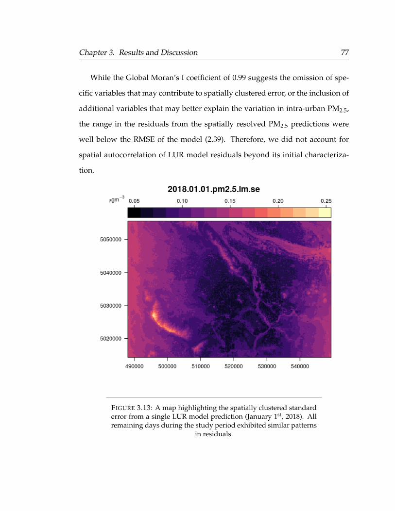
Chapter 3. Results and Discussion 77
While the Global Moran’s I coefficient of 0.99 suggests the omission of spe-
cific variables that may contribute to spatially clustered error, or the inclusion of
additional variables that may better explain the variation in intra-urban PM2.5,
the range in the residuals from the spatially resolved PM2.5 predictions were
well below the RMSE of the model (2.39). Therefore, we did not account for
spatial autocorrelation of LUR model residuals beyond its initial characteriza-
tion.
FIGURE 3.13: A map highlighting the spatially clustered standarderror from a single LUR model prediction (January 1st, 2018). Allremaining days during the study period exhibited similar patterns
in residuals.

Chapter 3. Results and Discussion 78
3.8 The Importance of Sensor Placement
While we were primarily focused on the anthropogenic drivers of fine-scale
PM2.5 spatial gradients, and the influence that vegetation may have on mitigat-
ing these exposures, ultimately no clear patterns between traffic or vegetation
variables could be established. Our assessment of the relative strengths of the
various sources and sinks of PM2.5 has shown that the median ambient back-
ground concentration provided by the ODEQ nephelometer network had the
strongest association with PM2.5, and the remaining variables were only weakly
associated. When comparing the relative strengths of the remaining variables,
the effect size of the temporal and spatiotemporal predictors was relatively
higher compared to the spatial variables, indicating that the spatial variation
of urban PM2.5 is primarily driven by meteorology and regional sources at the
50 m scale.
In addition to the observed spatial clustering in our model error, we found
the LUR model development to be extremely sensitive to the initial placement
of the PurpleAir response network. During the opportunistic ambient calibra-
tion phase, we explored several different time aggregations of the nephelometer
network in order to identify periods when PM2.5 was regionally homogeneous.
While we initially selected a 15-minute time resolution to evaluate the RSD of
the nephelometer network, we also explored a 1-hour resolution, which pro-
duced another set of reasonable correction factors. By implementing a coarser
time resolution during the opportunistic ambient calibration, we observed an
additional 9 sensors which passed our quality control criterion (R2 > 0.90 and

Chapter 3. Results and Discussion 79
n ≥ 50). This corresponded to approximately 5 additional locations (each node
contains both a primary and secondary sensor) and an increase in the total num-
ber of sensors from 61 to 70. The number of observations used during model
development subsequently rose from 11,546 to 12,388 during model develop-
ment. A new LUR model was developed with these data, and a different set of
predictors was selected (despite following the same predictor selection protocol
as with the previous model) (Table 3.5). For example, an additional proxy for
an anthropogenic source, railroad density, was determined to be a statistically
significant predictor with the new data. The log of the railroad density at 500
m produced a beta of 0.015. In addition, a vegetation variable, deciduous for-
est cover, was also identified as a significant predictor. The deciduous forest
predictor had a beta of 0.008, which was the lowest in this model. The relation-
ship between many of the spatial predictors and PM2.5 were weak, often with
beta coefficients below 0.05. Due to the spatial predictors being weakly associ-
ated with PM2.5, the addition or removal of a small subset of our response net-
work can lead to a major difference in the predictors selected for the final model.
When there are only a few sensors at each LULC to begin with, it becomes dif-
ficult to effectively capture the entire variation in each proxy, and model bias
increases. The correlations for many of the proxies for anthropogenic sources,
e.g. freeways, major arterials, railroads, developed LULC, and PM2.5 were tee-
tering above and below 0. The sign of the correlation coefficients for some pre-
dictors were observed to flip depending on whether the 15-minute or 1-hour
RSD nephelometer data were used to correct the response network. For exam-
ple, freeways at the 50 m buffer size flipped from a correlation coefficient of 0.01
Chapter 3. Results and Discussion 80
for the 15-minute data, to -0.01 for the 1-hour data. In reality, this relationship is
effectively null.
Patterns in PM2.5 were predominately explained by temporal factors over
spatial ones. Spatially, PM2.5 only varied by 0-5 µgm−3. Temporally, however,
PM2.5 levels were observed to increase by tens of micrograms per cubic meter
from day to day, especially during wildfire PM events in the summer months,
and temperature inversions in the winter months.
If there is a lack of representativeness with the air quality network used to
train the model, then model bias for predictions in unrepresented areas will be
higher. For example, if only a single sensor is located near railroad that has
elevated PM2.5 levels, then the model will predict that locations with a similar
railroad density will also be elevated, regardless of the train volume on each
particular rail.
In addition to the observed spatial clustering in our model error, we found
the LUR model development to be extremely sensitive to the initial placement
of the PurpleAir response network. During the opportunistic ambient calibra-
tion phase, we explored several different time resolutions of the nephelometer
network in order to identify periods when PM2.5 was regionally homogeneous.
While we initially selected a 15-minute time resolution to evaluate the RSD of
the nephelometer network, we also explored a 1-hour resolution, which pro-
duced another reasonable set of correction factors. By implementing this coarser
1-hour resolution during the opportunistic ambient calibration, we actually ob-
served an additional 9 sensors which passed our quality control criterion (R2
> 0.90 and n ≥ 50). This corresponded to approximately 5 additional locations
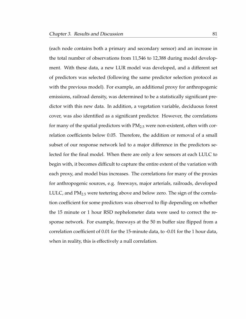
Chapter 3. Results and Discussion 81
(each node contains both a primary and secondary sensor) and an increase in
the total number of observations from 11,546 to 12,388 during model develop-
ment. With these data, a new LUR model was developed, and a different set
of predictors was selected (following the same predictor selection protocol as
with the previous model). For example, an additional proxy for anthropogenic
emissions, railroad density, was determined to be a statistically significant pre-
dictor with this new data. In addition, a vegetation variable, deciduous forest
cover, was also identified as a significant predictor. However, the correlations
for many of the spatial predictors with PM2.5 were non-existent, often with cor-
relation coefficients below 0.05. Therefore, the addition or removal of a small
subset of our response network led to a major difference in the predictors se-
lected for the final model. When there are only a few sensors at each LULC to
begin with, it becomes difficult to capture the entire extent of the variation with
each proxy, and model bias increases. The correlations for many of the proxies
for anthropogenic sources, e.g. freeways, major arterials, railroads, developed
LULC, and PM2.5 were teetering above and below zero. The sign of the correla-
tion coefficient for some predictors was observed to flip depending on whether
the 15 minute or 1 hour RSD nephelometer data were used to correct the re-
sponse network. For example, freeways at the 50 m buffer size flipped from a
correlation coefficient of 0.01 for the 15-minute data, to -0.01 for the 1 hour data,
when in reality, this is effectively a null correlation.
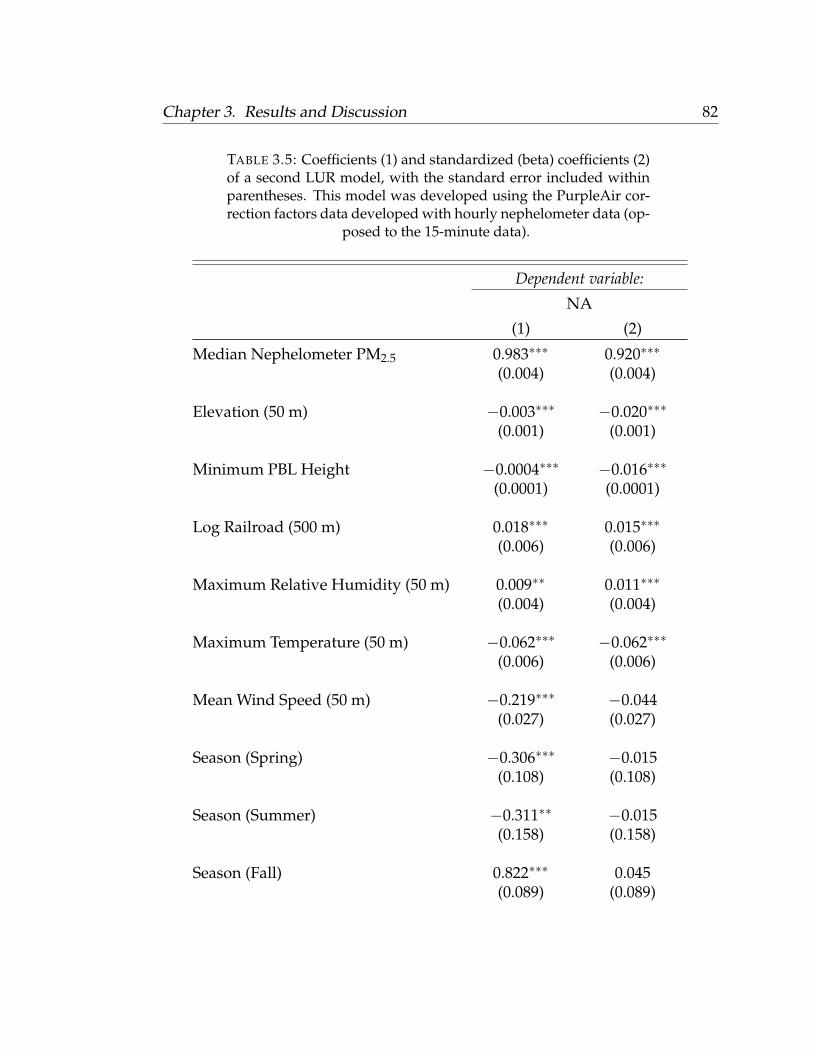
Chapter 3. Results and Discussion 82
TABLE 3.5: Coefficients (1) and standardized (beta) coefficients (2)of a second LUR model, with the standard error included withinparentheses. This model was developed using the PurpleAir cor-rection factors data developed with hourly nephelometer data (op-
posed to the 15-minute data).
Dependent variable:
NA
(1) (2)
Median Nephelometer PM2.5 0.983∗∗∗ 0.920∗∗∗
(0.004) (0.004)
Elevation (50 m) −0.003∗∗∗ −0.020∗∗∗
(0.001) (0.001)
Minimum PBL Height −0.0004∗∗∗ −0.016∗∗∗
(0.0001) (0.0001)
Log Railroad (500 m) 0.018∗∗∗ 0.015∗∗∗
(0.006) (0.006)
Maximum Relative Humidity (50 m) 0.009∗∗ 0.011∗∗∗
(0.004) (0.004)
Maximum Temperature (50 m) −0.062∗∗∗ −0.062∗∗∗
(0.006) (0.006)
Mean Wind Speed (50 m) −0.219∗∗∗ −0.044(0.027) (0.027)
Season (Spring) −0.306∗∗∗ −0.015(0.108) (0.108)
Season (Summer) −0.311∗∗ −0.015(0.158) (0.158)
Season (Fall) 0.822∗∗∗ 0.045(0.089) (0.089)
Chapter 3. Results and Discussion 83
Deciduous Forest (300 m) −3.661∗ −0.008(1.933) (1.933)
Developed Medium Intensity (300 m) 0.967∗∗∗ 0.023(0.255) (0.255)
Longitude −0.00001∗∗ −0.009∗∗∗
(0.00001) (0.00001)
Latitude 0.00001∗∗ 0.009∗∗∗
(0.00001) (0.00001)
Constant −32.782 0.000(26.091) (26.091)
Observations 8,671 8,671R2 0.879 0.879Adjusted R2 0.879 0.879Residual Std. Error (df = 8656) 2.878 2.878F Statistic (df = 14; 8656) 4,500.152∗∗∗ 4,500.152∗∗∗
Note: ∗p<0.1; ∗∗p<0.05; ∗∗∗p<0.01
3.9 Predictions
3.9.1 Land Use Regression
Predictions of a select day, October 10th, 2018, were mapped in order to charac-
terize the differences between the 1-hour RSD network and 15-minute RSD net-
work for both LUR and RF models. The spatial patterns from the 15-minute RSD
LUR model appear to approximate the underlying elevation and developed
medium intensity LULC predictors, despite the betas of these variables being
ranked only the 5th and 6th most associated with PM2.5. Since the general range
Chapter 3. Results and Discussion 84
of PM2.5 levels for any given day is primarily governed by the median neph-
elometer values, and other temporal scaling factors such as wind speed and
temperature, any remaining spatial heterogeneity is typically confined within a
± 5 µgm−3 range from the median. For example, the exact range in predicted
PM2.5 on this day was 6.25 - 8.62 µgm−3, a difference of only 2.37 µgm−3 from
the most to least polluted location. The 1-hour RSD LUR model captures simi-
lar patterns in elevation as the previous model, but the railroad and deciduous
forest variables suggest different hot spots and cold spots. For example, the
Western extent of the study area shows elevated PM2.5 levels due to the pres-
ence of railroads, whereas the previous model indicated this region should have
lower levels. In addition, small pockets of low PM2.5 concentrations scattered
throughout the region correspond to the presence of deciduous forest cover.
From the addition of these two spatial variables, the predicted range in PM2.5
concentration grew to 5.37 - 9.62 µgm−3, a 4.25 µgm−3 difference between most
and least polluted locations (Figure 3.14). The spatial heterogeneity in PM2.5 on
a given day is further limited when the model RMSE is taken into considera-
tion. The 15-minute RSD model, previously referred to as the ‘final model’, had
a RMSE of 2.39. When the RMSE is applied to the range in predicted PM2.5, it
becomes difficult to interpret most spatial patterns. For example, the cold spots
observed on October 10th, 2018 could potentially overlap with the hotspots, and
vice versa (e.g. 6.25 + 2.39 ≈ 8.62 − 2.39). In addition to the graphical assess-
ment, we regressed the 1-hour RSD model against the 15-minute RSD model
to further assess the relationship between the two models (Figure 3.15). The
15-minute RSD model (‘final model’) explained less than 1% of the variation in
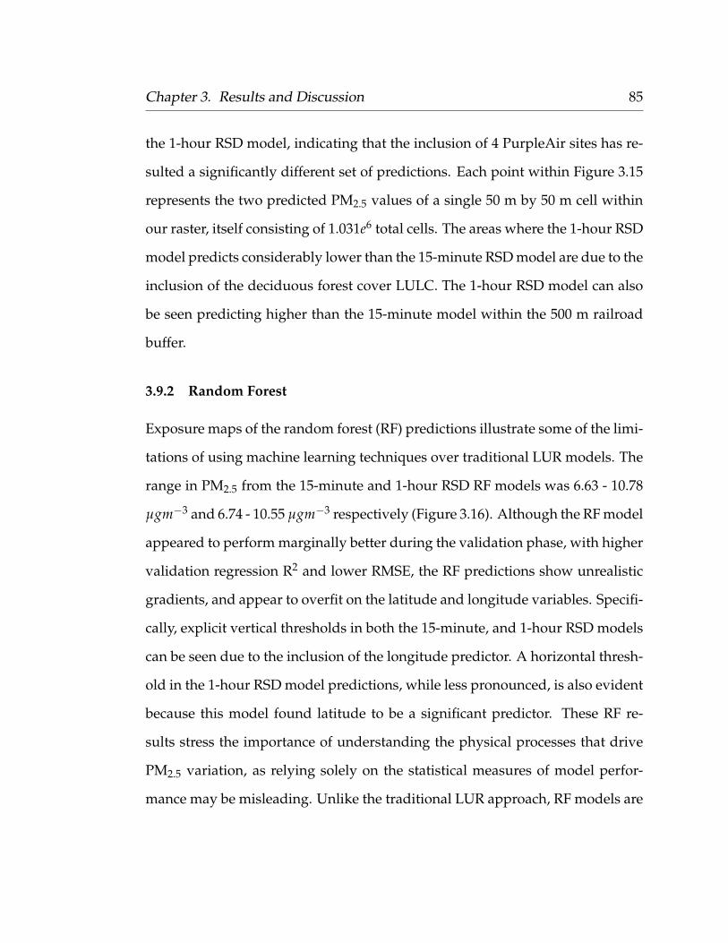
Chapter 3. Results and Discussion 85
the 1-hour RSD model, indicating that the inclusion of 4 PurpleAir sites has re-
sulted a significantly different set of predictions. Each point within Figure 3.15
represents the two predicted PM2.5 values of a single 50 m by 50 m cell within
our raster, itself consisting of 1.031e6 total cells. The areas where the 1-hour RSD
model predicts considerably lower than the 15-minute RSD model are due to the
inclusion of the deciduous forest cover LULC. The 1-hour RSD model can also
be seen predicting higher than the 15-minute model within the 500 m railroad
buffer.
3.9.2 Random Forest
Exposure maps of the random forest (RF) predictions illustrate some of the limi-
tations of using machine learning techniques over traditional LUR models. The
range in PM2.5 from the 15-minute and 1-hour RSD RF models was 6.63 - 10.78
µgm−3 and 6.74 - 10.55 µgm−3 respectively (Figure 3.16). Although the RF model
appeared to perform marginally better during the validation phase, with higher
validation regression R2 and lower RMSE, the RF predictions show unrealistic
gradients, and appear to overfit on the latitude and longitude variables. Specifi-
cally, explicit vertical thresholds in both the 15-minute, and 1-hour RSD models
can be seen due to the inclusion of the longitude predictor. A horizontal thresh-
old in the 1-hour RSD model predictions, while less pronounced, is also evident
because this model found latitude to be a significant predictor. These RF re-
sults stress the importance of understanding the physical processes that drive
PM2.5 variation, as relying solely on the statistical measures of model perfor-
mance may be misleading. Unlike the traditional LUR approach, RF models are

Chapter 3. Results and Discussion 86
essentially a black box and do not provide model coefficients necessary for inter-
preting the relative strengths of sources and sinks. As with many other machine
learning algorithms, random forest is a ‘data hungry’ technique, and relies on
a substantial training set in order to develop a robust stable model. While our
training set included more than 10,000 observations, these were generated from
a limited number (n ≈ 20) of physical locations which repeated over a 2-year
period. In comparison, the study area in which we are attempting to predict
includes over 1.031e6 individual grid cells at the 50 m resolution. We are likely
not capturing enough variation in each of our spatial predictors necessary to
develop a meaningful RF model for predicting intra-urban PM2.5.
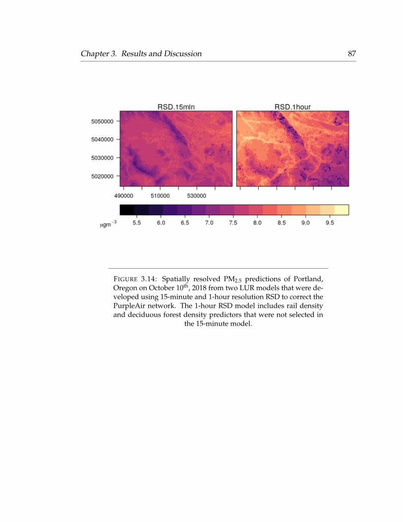
Chapter 3. Results and Discussion 87
FIGURE 3.14: Spatially resolved PM2.5 predictions of Portland,Oregon on October 10th, 2018 from two LUR models that were de-veloped using 15-minute and 1-hour resolution RSD to correct thePurpleAir network. The 1-hour RSD model includes rail densityand deciduous forest density predictors that were not selected in
the 15-minute model.
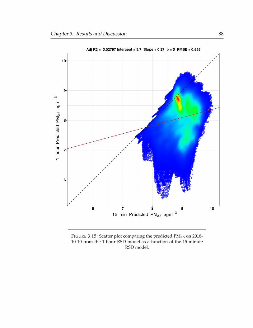
Chapter 3. Results and Discussion 88
FIGURE 3.15: Scatter plot comparing the predicted PM2.5 on 2018-10-10 from the 1-hour RSD model as a function of the 15-minute
RSD model.
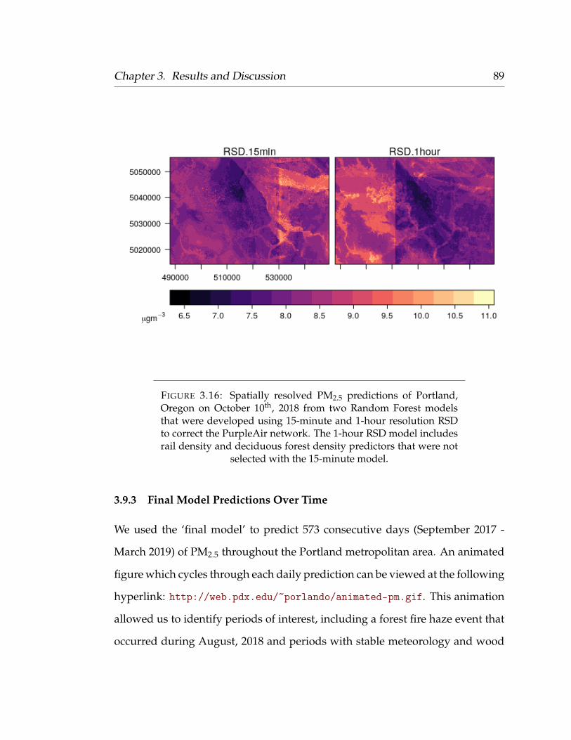
Chapter 3. Results and Discussion 89
FIGURE 3.16: Spatially resolved PM2.5 predictions of Portland,Oregon on October 10th, 2018 from two Random Forest modelsthat were developed using 15-minute and 1-hour resolution RSDto correct the PurpleAir network. The 1-hour RSD model includesrail density and deciduous forest density predictors that were not
selected with the 15-minute model.
3.9.3 Final Model Predictions Over Time
We used the ‘final model’ to predict 573 consecutive days (September 2017 -
March 2019) of PM2.5 throughout the Portland metropolitan area. An animated
figure which cycles through each daily prediction can be viewed at the following
hyperlink: http://web.pdx.edu/~porlando/animated-pm.gif. This animation
allowed us to identify periods of interest, including a forest fire haze event that
occurred during August, 2018 and periods with stable meteorology and wood

Chapter 3. Results and Discussion 90
burning in December, 2017. The spatial pattern appears to be relatively consis-
tent even on the most polluted days (Figures 3.17, 3.18).
FIGURE 3.17: Spatially resolved PM2.5 predictions of Portland,Oregon capturing a forest fire haze event that occurred between
August 17th - 25th, 2018 from the ‘final model’.
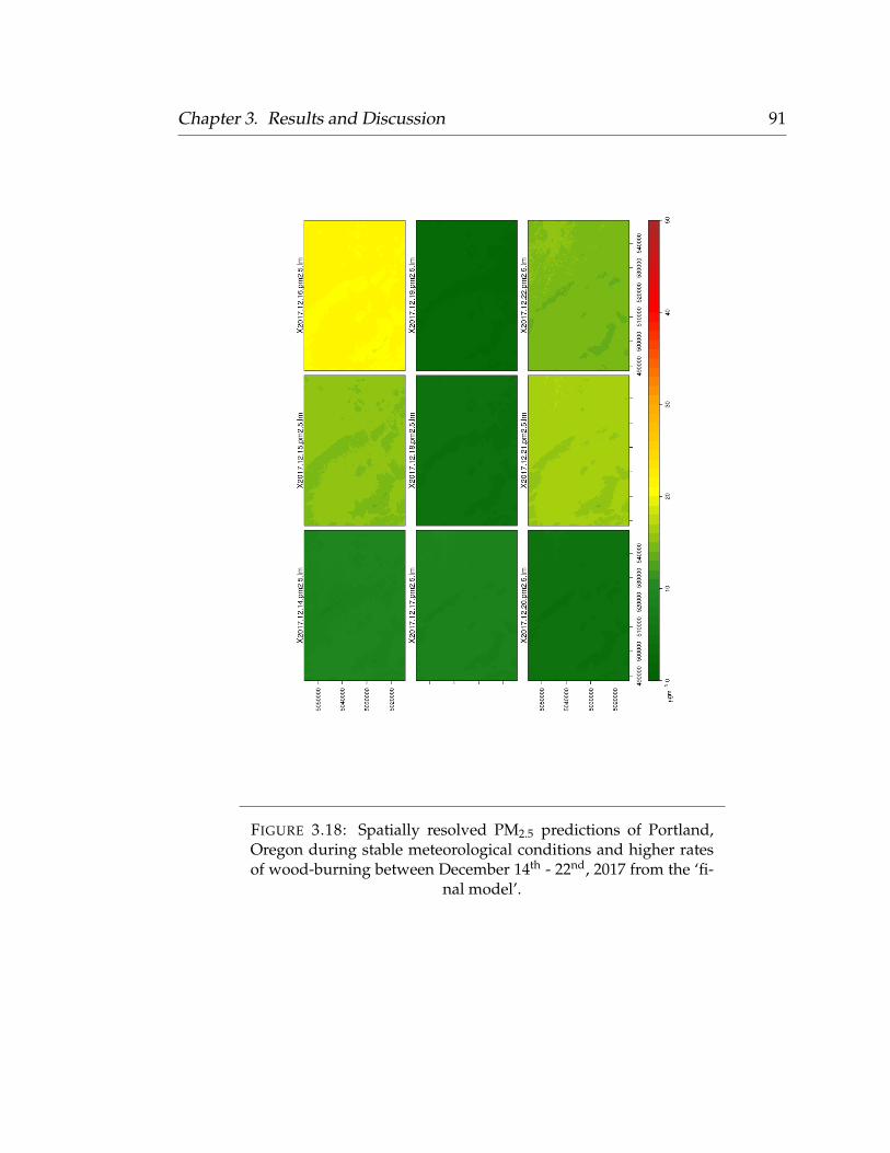
Chapter 3. Results and Discussion 91
FIGURE 3.18: Spatially resolved PM2.5 predictions of Portland,Oregon during stable meteorological conditions and higher ratesof wood-burning between December 14th - 22nd, 2017 from the ‘fi-
nal model’.

92
Chapter 4
Summary and Future Work
4.1 Summary
Spatially resolved PM2.5 concentrations at the intra-urban scale are not well de-
fined throughout US cities. This is due to the practical constraints of deploying
high-density networks using costly research-grade monitoring equipment, and
the focus on compliance at the regional scale from regulatory agencies. Monitor-
ing networks for PM2.5 are scarce, typically between 4-6 monitors per city, and
are often deliberately placed away from local sources in order to assess the am-
bient background concentration. The focus on compliance ultimately results in
the potential lack of representativeness of fixed air quality monitoring sites for
epidemiological studies, and limits studies which aim to characterize the poten-
tial role vegetation may play in mitigating PM2.5 exposure. Land use regression
techniques have been developed to account for the spatial heterogeneity of air
pollution sources within urban areas, in an effort to provide spatially resolved
exposure maps and identify the relative strengths of various sources and sinks.
This thesis explored the potential of using low-cost sensors for modeling spa-
tially resolved PM2.5 exposures within Portland, Oregon at a 50 m resolution
Chapter 4. Summary and Future Work 93
during a 2 year period. The low-cost sensor network increased the density of
the existing monitoring network by a factor of 5, enabling us to better character-
ize the potential patterns in sources and sinks throughout the region necessary
for producing spatially resolved PM2.5 exposures. However, we observed the
spatial predictors of PM2.5 to be only weakly associated with our response net-
work, relative to temporal scaling factors. This was not entirely surprising based
on the lack of fine-scale spatial variability in PM2.5 observed by previous stud-
ies (Karner, Eisinger, and Niemeier, 2010). In addition, the predicted range of
PM2.5 on a given day was typically within the RMSE of the LUR model. While
many air pollutants within cities have strong pollution gradients, typically de-
caying within 150 m - 200 m from the source, spatial patterns of PM2.5 are not
as distinct. As identified by Karner et al., gradients of PM2.5 with increasing
distance from traffic-related sources are mixed, and either decrease very grad-
ually or show no clear trend altogether (Karner, Eisinger, and Niemeier, 2010;
Kendrick, Koonce, and George, 2015). We could not identify a significant as-
sociation between our PurpleAir response network and any of the proxies for
traffic sources. The only anthropogenic source associated with PM2.5 was the
medium intensity developed LULC. This predictor was observed in both the 1-
hour and 15-minute RSD models, which may be a sign of developed land use
as a proxy for area sources. In contrast, no clear associations between proxies
for vegetation and PM2.5 were established during these initial modeling efforts,
and only a single vegetation LULC was identified during the additional 1-hour
RSD model. We characterized the sensitivity to initial sensor placement when
developing LUR models, as an addition of 4 sensors resulted in a considerably

Chapter 4. Summary and Future Work 94
different set of predictions throughout the study period. Despite the challenges
inherent to modeling spatially resolved PM2.5 with low-cost sensor data, this
thesis has developed a method for modeling intra-urban PM2.5 that can be gen-
eralized to many other cities, and produced a set of exposure maps which are
a notable improvement over the alternative exposures generated from spatially
interpolating the existing regulatory monitoring sites.
4.2 Future Work
We have developed a method for modeling spatially resolved PM2.5 at the sub-
neighborhood scale that can be applied to the remaining four cities within the
Canopy Continuum project. Future work will explore the associations between
a similar set of land use and meteorological predictors with each of the cor-
responding low-cost PM2.5 networks deployed throughout Albuquerque, New
Mexico, Boise, Idaho, Sacramento, California, and Tacoma, Washington. Since
these cities exhibit a varying degree of urban canopy cover, the development
of additional LUR models, and the resulting inter-city comparison may provide
further insights regarding the potential role of vegetation as a sink for PM2.5.
The inclusion of some additional key predictors should also be considered with
future models. As outlined by the ESCAPE project, traffic intensity data was
shown to be a crucial variable when predicting spatially resolved PM2.5 across
many European cities, where PM emissions are higher due to higher levels
of diesel engines, and study areas without local traffic intensity resulted in
poorer models. While we incorporated road density data of several road classes
(streets, arterials, freeways, etc.), the average annual daily traffic volume of
Chapter 4. Summary and Future Work 95
each road segment was not accounted for. In addition to traffic-intensity data,
the performance of ESCAPE models for predicting PM absorbance, a marker
of black carbon, were generally higher than that of PM2.5. This suggests that
additional monitoring networks may be required in order to characterize an-
thropogenic sources. While a substantial fraction of European private cars, and
nearly all middle and heavy duty vehicles, use diesel instead of gasoline, the
inclusion of PM absorbance within our LUR models may better reflect the im-
pact that mobile emissions have on fine-scale PM exposures within the urban
environment (Eeftens et al., 2012). The inclusion of particle number concentra-
tion, specifically of ultrafine PM, should also be considered in future modeling
efforts, as this pollutant is another proxy for emissions from local sources. The
two Plantower sensors inside each PurpleAir monitor provide additional mass
density measurements for PM1 and PM10. Plantower sensors are also capable
of measuring the number density of particles as small as 300 nm in diameter
(PM0.3). Future work should consider the inclusion of the various different PM
channels recorded by the PurpleAir network in effort to further characterize the
land-use and physical drivers of intra-urban PM variability (Appendix B).
Sensor placement, as we previously demonstrated, can have a cascading ef-
fect during model development. Two areas of improvement have been identi-
fied from these results: (1) a stratified sensor allocation method and (2) an alter-
native field calibration technique. A stratified sensor allocation method would
better approximate the true variation in each of the relevant spatial predictors.
The opportunistic placement of the PurpleAir sensors in Portland resulted in a
network which overrepresented urban areas near small streets, but lacked data

Chapter 4. Summary and Future Work 96
for both heavily trafficked and heavily vegetated areas, and did not fully cap-
ture the extent of the urban-rural gradient. A previous study which developed
fine-scale exposure maps of NO2 throughout Portland, Oregon relied on a strati-
fied random network of 144 passive samplers (Rao et al., 2014). Unfortunately, a
PM2.5 monitoring campaign of this caliber still poses many logistical challenges
even for low-cost sensors. The PurpleAir monitors are still limited by cost (a
PurpleNetwork with 144 sites would cost $36,000), power and telecommuni-
cation. Identifying remote locations that still provide access to an AC power
source and a WiFi connection would likely be prohibitive with a stratified ran-
dom sensor allocation. Our opportunistic ambient calibration method, while a
major improvement over using the uncorrected sensor data, recovered only 48%
of the PurpleAir network. An alternative field calibration method, for example
a pre- and post-study calibration of each individual sensor against a co-located
FRM in the field may return a higher data recovery rate, while enabling the
assessment of sensor drift overtime. This is especially important as we demon-
strated that the inclusion of a just a few sensors can have a significant impact on
the predicted spatial variability.

97
Bibliography
Abatzoglou, John T. (2013). “Development of gridded surface meteorological
data for ecological applications and modelling”. In: International Journal of
Climatology 33.1, pp. 121–131. ISSN: 1097-0088. DOI: 10.1002/joc.3413. URL:
https://rmets.onlinelibrary.wiley.com/doi/abs/10.1002/joc.3413
(visited on 06/25/2019).
Apte, Joshua S., Julian D. Marshall, Aaron J. Cohen, and Michael Brauer (July 7,
2015). “Addressing Global Mortality from Ambient PM2.5”. In: Environmen-
tal Science & Technology 49.13, pp. 8057–8066. ISSN: 0013-936X. DOI: 10.1021/
acs.est.5b01236. URL: https://doi.org/10.1021/acs.est.5b01236
(visited on 06/28/2019).
AQ-SPEC South Coast AQMD, OAR (Aug. 17, 2017a). Field Evaluation Purple Air
(PA-II) PM Sensor. AQ-SPEC. URL: http://www.aqmd.gov/aq-spec (visited
on 07/09/2019).
— (Aug. 17, 2017b). Laboratory Evaluation Purple Air (PA-II) PM Sensor. AQ-
SPEC. URL: http://www.aqmd.gov/aq-spec (visited on 07/09/2019).
Beckerman, Bernardo S., Michael Jerrett, Marc Serre, Randall V. Martin, Seung-
Jae Lee, Aaron van Donkelaar, Zev Ross, Jason Su, and Richard T. Burnett

Bibliography 98
(July 2, 2013). “A Hybrid Approach to Estimating National Scale Spatiotem-
poral Variability of PM2.5 in the Contiguous United States”. In: Environ-
mental Science & Technology 47.13, pp. 7233–7241. ISSN: 0013-936X. DOI: 10.
1021/es400039u. URL: https://doi.org/10.1021/es400039u (visited on
07/07/2019).
Beckett, K Paul, Peter Freer-Smith, and Gail Taylor (2000). “Effective Tree
Species for Local Air Quality Management”. In: p. 8.
Beckett, K. Paul, P. H. Freer-Smith, and Gail Taylor (2000). “Particulate pollution
capture by urban trees: effect of species and windspeed”. In: Global Change
Biology 6.8, pp. 995–1003. ISSN: 1365-2486. DOI: 10.1046/j.1365-2486.2000.
00376.x. URL: https://onlinelibrary.wiley.com/doi/abs/10.1046/j.
1365-2486.2000.00376.x (visited on 07/04/2019).
Bell, Janice F., Jeffrey S. Wilson, and Gilbert C. Liu (Dec. 1, 2008). “Neighborhood
Greenness and 2-Year Changes in Body Mass Index of Children and Youth”.
In: American Journal of Preventive Medicine 35.6, pp. 547–553. ISSN: 0749-3797.
DOI: 10.1016/j.amepre.2008.07.006. URL: http://www.sciencedirect.
com/science/article/pii/S0749379708007344 (visited on 07/04/2019).
Bivand, Roger, Tim Keitt, and Barry Rowlingson (2019). rgdal: Bindings for the
’Geospatial’ Data Abstraction Library. URL: https://CRAN.R-project.org/
package=rgdal.
Bivand, Roger and Colin Rundel (2019). rgeos: Interface to Geometry Engine - Open
Source (’GEOS’). URL: https://CRAN.R-project.org/package=rgeos.

Bibliography 99
Breiman, Leo (Oct. 1, 2001). “Random Forests”. In: Machine Learning 45.1, pp. 5–
32. ISSN: 1573-0565. DOI: 10.1023/A:1010933404324. URL: https://doi.
org/10.1023/A:1010933404324 (visited on 07/10/2019).
Briggs, David J., Cornelis de Hoogh, John Gulliver, John Wills, Paul Elliott, Si-
mon Kingham, and Kirsty Smallbone (May 15, 2000). “A regression-based
method for mapping traffic-related air pollution: application and testing
in four contrasting urban environments”. In: Science of The Total Environ-
ment 253.1, pp. 151–167. ISSN: 0048-9697. DOI: 10.1016/S0048- 9697(00)
00429-0. URL: http://www.sciencedirect.com/science/article/pii/
S0048969700004290 (visited on 06/26/2019).
Brokamp, Cole, Roman Jandarov, M. B. Rao, Grace LeMasters, and Patrick Ryan
(Feb. 1, 2017). “Exposure assessment models for elemental components of
particulate matter in an urban environment: A comparison of regression and
random forest approaches”. In: Atmospheric Environment 151, pp. 1–11. ISSN:
1352-2310. DOI: 10.1016/j.atmosenv.2016.11.066. URL: http://www.
sciencedirect.com/science/article/pii/S1352231016309566 (visited on
07/17/2019).
Brugge, Doug, John L. Durant, and Christine Rioux (Aug. 9, 2007). “Near-
highway pollutants in motor vehicle exhaust: A review of epidemiologic
evidence of cardiac and pulmonary health risks”. In: Environmental Health
6.1, p. 23. ISSN: 1476-069X. DOI: 10.1186/1476- 069X- 6- 23. URL: https:
//doi.org/10.1186/1476-069X-6-23 (visited on 07/03/2019).
Brunekreef, B. and S. T. Holgate (Oct. 19, 2002). “Air pollution and health”. In:
The Lancet 360.9341, pp. 1233–1242. ISSN: 0140-6736. DOI: 10.1016/S0140-

Bibliography 100
6736(02 ) 11274 - 8. URL: http : / / www . sciencedirect . com / science /
article/pii/S0140673602112748 (visited on 06/22/2019).
Bureau, US Census (2012). “Patterns of metropolitan and micropolitan popula-
tion change: 2000 to 2010”. In: Census Special Reports.
Cheng, Joe, Bhaskar Karambelkar, and Yihui Xie (2018). leaflet: Create Interactive
Web Maps with the JavaScript ’Leaflet’ Library. URL: https://CRAN.R-project.
org/package=leaflet.
Chudnovsky, A. A., P. Koutrakis, I. Kloog, S. Melly, F. Nordio, A. Lyapustin, Y.
Wang, and J. Schwartz (June 1, 2014). “Fine particulate matter predictions us-
ing high resolution Aerosol Optical Depth (AOD) retrievals”. In: Atmospheric
Environment 89, pp. 189–198. ISSN: 1352-2310. DOI: 10.1016/j.atmosenv.
2014.02.019. URL: http://www.sciencedirect.com/science/article/
pii/S1352231014001150 (visited on 03/19/2019).
Chun, Youngsin, Jiyoung Kim, Jae Cheon Choi, Kyung On Boo, Sung Nam
Oh, and Meehye Lee (May 1, 2001). “Characteristic number size distribu-
tion of aerosol during Asian dust period in Korea”. In: Atmospheric Environ-
ment 35.15, pp. 2715–2721. ISSN: 1352-2310. DOI: 10.1016/S1352-2310(00)
00404-0. URL: http://www.sciencedirect.com/science/article/pii/
S1352231000004040 (visited on 07/03/2019).
Cohen, A. J., R. H. Anderson, B. Ostro, K. D. Pandey, M. Krzyzanowski, N Kün-
zli, K. Gutschmidt, A. C. Pope III, I Romieu, J.M. Samet, and K. Smith (July 1,
2005). “The Global Burden of Disease Due to Outdoor Air Pollution”. In:
Journal of Toxicology and Environmental Health, Part A 68.13, pp. 1301–1307.

Bibliography 101
ISSN: 1528-7394. DOI: 10.1080/15287390590936166. URL: https://doi.org/
10.1080/15287390590936166 (visited on 06/22/2019).
Daly, C. (May 2006). “Guidelines for assessing the suitability of spatial climate
data sets”. In: International Journal of Climatology 26.6, pp. 707–721. ISSN: 0899-
8418, 1097-0088. DOI: 10.1002/joc.1322. URL: http://doi.wiley.com/10.
1002/joc.1322 (visited on 06/25/2019).
Defays, D. (Jan. 1, 1977). “An efficient algorithm for a complete link method”.
In: The Computer Journal 20.4, pp. 364–366. ISSN: 0010-4620. DOI: 10.1093/
comjnl/20.4.364. URL: https://academic.oup.com/comjnl/article/20/
4/364/393966 (visited on 07/08/2019).
Didan, K (2015a). MOD13A2 MODIS/Terra Vegetation Indices 16-Day L3 Global
1km SIN Grid V006, NASA EOSDIS LP DAAC.
Didan, K. (2015b). “MOD13Q1 MODIS/Terra vegetation indices 16-day L3
global 250m SIN grid V006”. In: NASA EOSDIS Land Processes DAAC.
Dockery, D.W., A.C. Pope III, X. Xu, J. D. Spengler, J. H. Ware, Martha E.
Fay, Benjamin G. Ferris, and Frank E. Speizer (Dec. 9, 1993). “An Asso-
ciation between Air Pollution and Mortality in Six U.S. Cities”. In: New
England Journal of Medicine 329.24, pp. 1753–1759. ISSN: 0028-4793. DOI:
10 . 1056 / NEJM199312093292401. URL: https : / / doi . org / 10 . 1056 /
NEJM199312093292401 (visited on 06/22/2019).
Donovan, Geoffrey H., Yvonne L. Michael, David T. Butry, Amy D. Sullivan,
and John M. Chase (Jan. 1, 2011). “Urban trees and the risk of poor birth out-
comes”. In: Health & Place. Health Geographies of Voluntarism 17.1, pp. 390–
393. ISSN: 1353-8292. DOI: 10.1016/j.healthplace.2010.11.004. URL: http:

Bibliography 102
//www.sciencedirect.com/science/article/pii/S1353829210001656
(visited on 07/04/2019).
Doxsey-Whitfield, Erin, Kytt MacManus, Susana B. Adamo, Linda Pistolesi,
John Squires, Olena Borkovska, and Sandra R. Baptista (July 3, 2015). “Tak-
ing Advantage of the Improved Availability of Census Data: A First Look at
the Gridded Population of the World, Version 4”. In: Papers in Applied Geogra-
phy 1.3, pp. 226–234. ISSN: 2375-4931. DOI: 10.1080/23754931.2015.1014272.
URL: https : / / doi . org / 10 . 1080 / 23754931 . 2015 . 1014272 (visited on
07/08/2019).
Eeftens, Marloes, Rob Beelen, Kees de Hoogh, Tom Bellander, Giulia Cesaroni,
Marta Cirach, Christophe Declercq, Audrius Dedele, Evi Dons, Audrey de
Nazelle, Konstantina Dimakopoulou, Kirsten Eriksen, Grégoire Falq, Paul
Fischer, Claudia Galassi, Regina Gražuleviciene, Joachim Heinrich, Barbara
Hoffmann, Michael Jerrett, Dirk Keidel, Michal Korek, Timo Lanki, Sarah
Lindley, Christian Madsen, Anna Mölter, Gizella Nádor, Mark Nieuwenhui-
jsen, Michael Nonnemacher, Xanthi Pedeli, Ole Raaschou-Nielsen, Evridiki
Patelarou, Ulrich Quass, Andrea Ranzi, Christian Schindler, Morgane
Stempfelet, Euripides Stephanou, Dorothea Sugiri, Ming-Yi Tsai, Tarja Yli-
Tuomi, Mihály J Varró, Danielle Vienneau, Stephanie von Klot, Kathrin Wolf,
Bert Brunekreef, and Gerard Hoek (Oct. 16, 2012). “Development of Land
Use Regression Models for PM2.5, PM2.5 Absorbance, PM10 and PMcoarse
in 20 European Study Areas; Results of the ESCAPE Project”. In: Environ-
mental Science & Technology 46.20, pp. 11195–11205. ISSN: 0013-936X. DOI:

Bibliography 103
10.1021/es301948k. URL: https://doi.org/10.1021/es301948k (visited on
11/16/2018).
EPA, US (2004). “Air quality criteria for particulate matter”. In: US Environmen-
tal Protection Agency, Research Triangle Park.
Fann, N., A. D. Lamson, S. C. Anenberg, K. Wesson, D. Risley, and B. J. Hubbell
(Jan. 1, 2012). “Estimating the National Public Health Burden Associated
with Exposure to Ambient PM2.5 and Ozone”. In: Risk Analysis 32.1, pp. 81–
95. ISSN: 0272-4332. DOI: 10.1111/j.1539-6924.2011.01630.x. URL: https:
//onlinelibrary.wiley.com/doi/full/10.1111/j.1539-6924.2011.
01630.x (visited on 06/22/2019).
Fenger, Jes (Dec. 1, 1999). “Urban air quality”. In: Atmospheric Environment
33.29, pp. 4877–4900. ISSN: 1352-2310. DOI: 10 . 1016 / S1352 - 2310(99 )
00290-3. URL: http://www.sciencedirect.com/science/article/pii/
S1352231099002903 (visited on 07/03/2019).
Fox, John, Gregor Gorjanc Friendly, Spencer Graves, Richard Heiberger,
Georges Monette, Henric Nilsson, Brian Ripley, Sanford Weisberg, Main-
tainer John Fox, and MASS Suggests (2007). “The car package”. In: R Foun-
dation for Statistical Computing.
Freer-Smith, P. H., K. P. Beckett, and Gail Taylor (Jan. 1, 2005). “Deposition
velocities to Sorbus aria, Acer campestre, Populus deltoides × trichocarpa
‘Beaupré’, Pinus nigra and × Cupressocyparis leylandii for coarse, fine and
ultra-fine particles in the urban environment”. In: Environmental Pollution
133.1, pp. 157–167. ISSN: 0269-7491. DOI: 10 . 1016 / j . envpol . 2004 . 03 .

Bibliography 104
031. URL: http : / / www . sciencedirect . com / science / article / pii /
S0269749104001228 (visited on 07/04/2019).
Freer-Smith, P. H., A. A. El-Khatib, and Gail Taylor (June 1, 2004). “Capture of
Particulate Pollution by Trees: A Comparison of Species Typical of Semi-Arid
Areas (Ficus Nitida and Eucalyptus Globulus) with European and North
American Species”. In: Water, Air, and Soil Pollution 155.1, pp. 173–187. ISSN:
1573-2932. DOI: 10.1023/B:WATE.0000026521.99552.fd. URL: https://doi.
org/10.1023/B:WATE.0000026521.99552.fd (visited on 07/04/2019).
Fritsch, F. and R. Carlson (Apr. 1, 1980). “Monotone Piecewise Cubic Interpola-
tion”. In: SIAM Journal on Numerical Analysis 17.2, pp. 238–246. ISSN: 0036-
1429. DOI: 10.1137/0717021. URL: https://epubs.siam.org/doi/abs/10.
1137/0717021 (visited on 06/25/2019).
Gilliland Frank, Avol Ed, Kinney Patrick, Jerrett Michael, Dvonch Timothy, Lur-
mann Frederick, Buckley Timothy, Breysse Patrick, Keeler Gerald, de Villiers
Tracy, and McConnell Rob (Oct. 1, 2005). “Air Pollution Exposure Assess-
ment for Epidemiologic Studies of Pregnant Women and Children: Lessons
Learned from the Centers for Children’s Environmental Health and Disease
Prevention Research”. In: Environmental Health Perspectives 113.10, pp. 1447–
1454. DOI: 10.1289/ehp.7673. URL: https://ehp.niehs.nih.gov/doi/
full/10.1289/ehp.7673 (visited on 07/07/2019).
Harrison, Roy M., Alan M. Jones, and Roger Barrowcliffe (Dec. 1, 2004). “Field
study of the influence of meteorological factors and traffic volumes upon
suspended particle mass at urban roadside sites of differing geometries”.
In: Atmospheric Environment 38.37, pp. 6361–6369. ISSN: 1352-2310. DOI: 10.

Bibliography 105
1016/j.atmosenv.2004.07.030. URL: http://www.sciencedirect.com/
science/article/pii/S1352231004007058 (visited on 06/28/2019).
Hastie, Trevor, Robert Tibshirani, Jerome Friedman, and James Franklin (2005).
“The elements of statistical learning: data mining, inference and prediction”.
In: The Mathematical Intelligencer 27.2, pp. 83–85.
Hijmans, Robert J. (2019). raster: Geographic Data Analysis and Modeling. URL:
https://CRAN.R-project.org/package=raster.
Hoek, Gerard, Bert Brunekreef, Arnoud Verhoeff, Joop van Wijnen, and Paul
Fischer (Aug. 1, 2000). “Daily Mortality and Air Pollution in the Nether-
lands”. In: Journal of the Air & Waste Management Association 50.8, pp. 1380–
1389. ISSN: 1096-2247. DOI: 10.1080/10473289.2000.10464182. URL: https:
//doi.org/10.1080/10473289.2000.10464182 (visited on 07/03/2019).
Hoek, Gerard, Bert Brunekreef, Sandra Goldbohm, Paul Fischer, and Piet A van
den Brandt (Oct. 19, 2002). “Association between mortality and indicators of
traffic-related air pollution in the Netherlands: a cohort study”. In: The Lancet
360.9341, pp. 1203–1209. ISSN: 0140-6736. DOI: 10.1016/S0140- 6736(02)
11280-3. URL: http://www.sciencedirect.com/science/article/pii/
S0140673602112803 (visited on 07/03/2019).
Hoek, Gerard, Rob Beelen, Kees de Hoogh, Danielle Vienneau, John Gulliver,
Paul Fischer, and David Briggs (Oct. 1, 2008). “A review of land-use regres-
sion models to assess spatial variation of outdoor air pollution”. In: Atmo-
spheric Environment 42.33, pp. 7561–7578. ISSN: 1352-2310. DOI: 10.1016/j.
atmosenv.2008.05.057. URL: http://www.sciencedirect.com/science/
article/pii/S1352231008005748 (visited on 07/05/2019).

Bibliography 106
Homer, C., J. Dewitz, L. Yang, S. Jin, P. Danielson, G. Xian, J. Coul-
ston, N. Herold, J. Wickham, and K. Megown (2015). “Completion of
the 2011 National Land Cover Database for the conterminous United
States–representing a decade of land cover change information”. In: Pho-
togrammetric Engineering & Remote Sensing 81.5, pp. 345–354.
Jeanjean, A. P. R., P. S. Monks, and R. J. Leigh (Dec. 1, 2016). “Modelling the
effectiveness of urban trees and grass on PM2.5 reduction via dispersion and
deposition at a city scale”. In: Atmospheric Environment 147, pp. 1–10. ISSN:
1352-2310. DOI: 10.1016/j.atmosenv.2016.09.033. URL: http://www.
sciencedirect.com/science/article/pii/S1352231016307336 (visited on
07/05/2019).
Jerrett, M., M. A. Arain, P. Kanaroglou, B. Beckerman, D. Crouse, N. L. Gilbert,
J. R. Brook, N. Finkelstein, and M. M. Finkelstein (Feb. 1, 2007). “Modeling
the Intraurban Variability of Ambient Traffic Pollution in Toronto, Canada”.
In: Journal of Toxicology and Environmental Health, Part A 70.3, pp. 200–212.
ISSN: 1528-7394. DOI: 10.1080/15287390600883018. URL: https://doi.org/
10.1080/15287390600883018 (visited on 07/07/2019).
Jerrett, Michael, Richard T Burnett, Renjun Ma, C Arden Pope III, Daniel
Krewski, K Bruce Newbold, George Thurston, Yuanli Shi, Norm Finkelstein,
Eugenia E Calle, and others (2005). “Spatial analysis of air pollution and mor-
tality in Los Angeles”. In: Epidemiology, pp. 727–736.
Jerrett, Michael, Shankardass Ketan, Berhane Kiros, Gauderman W. James,
Künzli Nino, Avol Edward, Gilliland Frank, Lurmann Fred, Molitor Jassy
N., Molitor John T., Thomas Duncan C., Peters John, and McConnell Rob

Bibliography 107
(Oct. 1, 2008). “Traffic-Related Air Pollution and Asthma Onset in Children:
A Prospective Cohort Study with Individual Exposure Measurement”. In:
Environmental Health Perspectives 116.10, pp. 1433–1438. DOI: 10.1289/ehp.
10968. URL: https://ehp.niehs.nih.gov/doi/10.1289/ehp.10968 (visited
on 07/04/2019).
Karner, Alex A., Douglas S. Eisinger, and Deb A. Niemeier (July 15, 2010).
“Near-Roadway Air Quality: Synthesizing the Findings from Real-World
Data”. In: Environmental Science & Technology 44.14, pp. 5334–5344. ISSN:
0013-936X. DOI: 10.1021/es100008x. URL: https://doi.org/10.1021/
es100008x (visited on 06/28/2019).
Kendrick, Christine M., Peter Koonce, and Linda A. George (Dec. 1, 2015). “Di-
urnal and seasonal variations of NO, NO2 and PM2.5 mass as a function
of traffic volumes alongside an urban arterial”. In: Atmospheric Environment
122, pp. 133–141. ISSN: 1352-2310. DOI: 10.1016/j.atmosenv.2015.09.
019. URL: http : / / www . sciencedirect . com / science / article / pii /
S1352231015303605 (visited on 07/03/2019).
Kim, Y. S. (2004). “Dust particles in the free atmosphere over desert areas on
the Asian continent: Measurements from summer 2001 to summer 2002
with balloon-borne optical particle counter and lidar, Dunhuang, China”.
In: Journal of Geophysical Research 109 (D19). ISSN: 0148-0227. DOI: 10.1029/
2002JD003269. URL: http://doi.wiley.com/10.1029/2002JD003269 (visited
on 07/03/2019).
Kloog, I., B. Ridgway, P. Koutrakis, B. A. Coull, and J. D. Schwartz (July 2013).
“Long- and Short-Term Exposure to PM2.5 and Mortality”. In: Epidemiology

Bibliography 108
(Cambridge, Mass.) 24.4, pp. 555–561. ISSN: 1044-3983. DOI: 10.1097/EDE.
0b013e318294beaa. URL: https://www.ncbi.nlm.nih.gov/pmc/articles/
PMC4372644/ (visited on 06/22/2019).
Kobayashi, Hiroshi, Masahiko Hayashi, Koichi Shiraishi, Yoshinobu Nakura,
Takayuki Enomoto, Kazuhiko Miura, Hiroshi Takahashi, Yasuhito Igarashi,
Hiroaki Naoe, Naoki Kaneyasu, Tomoaki Nishizawa, and Nobuo Sugimoto
(Nov. 1, 2014). “Development of a polarization optical particle counter capa-
ble of aerosol type classification”. In: Atmospheric Environment 97, pp. 486–
492. ISSN: 1352-2310. DOI: 10.1016/j.atmosenv.2014.05.006. URL: http:
//www.sciencedirect.com/science/article/pii/S1352231014003537
(visited on 07/03/2019).
Kohli, Rajiv and Kashmiri L. Mittal (Nov. 12, 2015). Developments in Surface Con-
tamination and Cleaning, Vol. 1: Fundamentals and Applied Aspects. Google-
Books-ID: WZDmBQAAQBAJ. William Andrew. 898 pp. ISBN: 978-0-323-
31270-7.
Le Tertre, A., S. Medina, E. Samoli, B. Forsberg, P. Michelozzi, A. Boumghar, J.
M. Vonk, A. Bellini, R. Atkinson, J. G. Ayres, J. Sunyer, J. Schwartz, and K.
Katsouyanni (Oct. 1, 2002). “Short-term effects of particulate air pollution on
cardiovascular diseases in eight European cities”. In: Journal of Epidemiology
& Community Health 56.10, pp. 773–779. ISSN: 0143-005X, 1470-2738. DOI: 10.
1136/jech.56.10.773. URL: https://jech.bmj.com/content/56/10/773
(visited on 06/22/2019).

Bibliography 109
Liaw, Andy and Matthew Wiener (2002). “Classification and Regression by ran-
domForest”. In: R News 2.3, pp. 18–22. URL: https://CRAN.R-project.org/
doc/Rnews/.
Lim, Stephen S, Theo Vos, Abraham D Flaxman, Goodarz Danaei, Kenji
Shibuya, Heather Adair-Rohani, Mohammad A AlMazroa, Markus Amann,
H Ross Anderson, Kathryn G Andrews, and others (2012). “A comparative
risk assessment of burden of disease and injury attributable to 67 risk factors
and risk factor clusters in 21 regions, 1990–2010: a systematic analysis for the
Global Burden of Disease Study 2010”. In: The lancet 380.9859, pp. 2224–2260.
Liu, Chao, Barron H. Henderson, Dongfang Wang, Xinyuan Yang, and Zhong-
ren Peng (Sept. 15, 2016). “A land use regression application into assessing
spatial variation of intra-urban fine particulate matter (PM2.5) and nitro-
gen dioxide (NO2) concentrations in City of Shanghai, China”. In: Science
of The Total Environment 565, pp. 607–615. ISSN: 0048-9697. DOI: 10.1016/j.
scitotenv.2016.03.189. URL: http://www.sciencedirect.com/science/
article/pii/S004896971630609X (visited on 07/07/2019).
Maas, J., R. A. Verheij, S. de Vries, P. Spreeuwenberg, F. G. Schellevis, and P.
P. Groenewegen (Dec. 1, 2009). “Morbidity is related to a green living envi-
ronment”. In: Journal of Epidemiology & Community Health 63.12, pp. 967–973.
ISSN: 0143-005X, 1470-2738. DOI: 10.1136/jech.2008.079038. URL: https:
//jech.bmj.com/content/63/12/967 (visited on 07/04/2019).
Mattiuzzi, Matteo and Florian Detsch (2019). MODIS: Acquisition and Processing
of MODIS Products. URL: https://CRAN.R-project.org/package=MODIS.

Bibliography 110
Mesinger, F., G. DiMego, E. Kalnay, K. Mitchell, P. C. Shafran, W. Ebisuzaki, D.
Jovic, J. Woollen, E. Rogers, E.H. Berbery, M. B. Ek, Y. Fan, R. Grumbine,
W. Higgins, H. Li, Y. Lin, G. Manikin, D. Parrish, and W. Shi (Mar. 1, 2006).
“North American Regional Reanalysis”. In: Bulletin of the American Meteoro-
logical Society 87.3, pp. 343–360. ISSN: 0003-0007. DOI: 10.1175/BAMS-87-3-
343. URL: https://journals.ametsoc.org/doi/abs/10.1175/BAMS-87-3-
343 (visited on 06/25/2019).
Mitchell, Richard and Frank Popham (Aug. 1, 2007). “Greenspace, urbanity and
health: relationships in England”. In: Journal of Epidemiology & Community
Health 61.8, pp. 681–683. ISSN: 0143-005X, 1470-2738. DOI: 10.1136/jech.
2006.053553. URL: https://jech.bmj.com/content/61/8/681 (visited on
07/04/2019).
NASA (2009). ASTER Global Digital Elevation Map. URL: https://asterweb.jpl.
nasa.gov/gdem.asp (visited on 07/10/2019).
Nowak, David J., Daniel E. Crane, and Jack C. Stevens (Apr. 3, 2006). “Air pol-
lution removal by urban trees and shrubs in the United States”. In: Urban
Forestry & Urban Greening 4.3, pp. 115–123. ISSN: 1618-8667. DOI: 10.1016/
j.ufug.2006.01.007. URL: http://www.sciencedirect.com/science/
article/pii/S1618866706000173 (visited on 07/04/2019).
Nowak, David J. and Eric J. Greenfield (July 1, 2012). “Tree and impervious
cover in the United States”. In: Landscape and Urban Planning 107.1, pp. 21–
30. ISSN: 0169-2046. DOI: 10.1016/j.landurbplan.2012.04.005. URL: http:
//www.sciencedirect.com/science/article/pii/S0169204612001193
(visited on 07/04/2019).

Bibliography 111
Nowak, David J., Satoshi Hirabayashi, Allison Bodine, and Robert Hoehn
(July 1, 2013). “Modeled PM2.5 removal by trees in ten U.S. cities and as-
sociated health effects”. In: Environmental Pollution 178, pp. 395–402. ISSN:
0269-7491. DOI: 10 . 1016 / j . envpol . 2013 . 03 . 050. URL: http : / / www .
sciencedirect.com/science/article/pii/S0269749113001838 (visited
on 07/04/2019).
Nyberg, Fredrik, Per Gustavsson, Lars Järup, Tom Bellander, Niklas Berglind,
Robert Jakobsson, and Göran Pershagen (2000). “Urban Air Pollution and
Lung Cancer in Stockholm”. In: Epidemiology 11.5, pp. 487–495. ISSN: 1044-
3983. URL: https : / / www . jstor . org / stable / 3703988 (visited on
07/03/2019).
Oberdorster, G., E. Oberdorster, and J. Oberdorster (2005). Nanotoxicology: an
emerging discipline evolving from studies of ultrafine particles. Environ Health Per-
spect 113:823–839.
Oregon Metro (2018). RLIS Discovery: Home. Regional Land Information System.
URL: http://rlisdiscovery.oregonmetro.gov/ (visited on 07/10/2019).
Pebesma, Edzer (2018). “Simple Features for R: Standardized Support for Spatial
Vector Data”. In: The R Journal 10.1, pp. 439–446. DOI: 10.32614/RJ-2018-
009. URL: https://doi.org/10.32614/RJ-2018-009.
Pebesma, Edzer J. and Roger S. Bivand (Nov. 2005). “Classes and methods for
spatial data in R”. In: R News 5.2, pp. 9–13. URL: https://CRAN.R-project.
org/doc/Rnews/.

Bibliography 112
Pope, A. C. III and D. W. Dockery (June 1, 2006). “Health Effects of Fine Particu-
late Air Pollution: Lines that Connect”. In: Journal of the Air & Waste Manage-
ment Association 56.6, pp. 709–742. ISSN: 1096-2247. DOI: 10.1080/10473289.
2006.10464485. URL: https://doi.org/10.1080/10473289.2006.10464485
(visited on 06/22/2019).
Pope, C. Arden III, Richard T. Burnett, Michael J. Thun, Eugenia E. Calle, Daniel
Krewski, Kazuhiko Ito, and George D. Thurston (Mar. 6, 2002). “Lung Can-
cer, Cardiopulmonary Mortality, and Long-term Exposure to Fine Particu-
late Air Pollution”. In: JAMA 287.9, pp. 1132–1141. ISSN: 0098-7484. DOI:
10.1001/jama.287.9.1132. URL: https://jamanetwork.com/journals/
jama/fullarticle/194704 (visited on 07/06/2019).
Pullman, Marcie (Aug. 21, 2008). “Conifer PM2.5 Deposition and Resuspension
in Wind and Rain Events”. In: URL: https : / / ecommons . cornell . edu /
handle/1813/11239 (visited on 07/04/2019).
R Core Team (2019). R: A Language and Environment for Statistical Computing.
Vienna, Austria: R Foundation for Statistical Computing. URL: https://www.
R-project.org/.
Rao, Meenakshi, Linda A. George, Todd N. Rosenstiel, Vivek Shandas, and
Alexis Dinno (Nov. 1, 2014). “Assessing the relationship among urban
trees, nitrogen dioxide, and respiratory health”. In: Environmental Pollution
194, pp. 96–104. ISSN: 0269-7491. DOI: 10 . 1016 / j . envpol . 2014 . 07 .
011. URL: http : / / www . sciencedirect . com / science / article / pii /
S0269749114003030 (visited on 03/26/2019).

Bibliography 113
Ross, Zev, Michael Jerrett, Kazuhiko Ito, Barbara Tempalski, and George D.
Thurston (Apr. 1, 2007). “A land use regression for predicting fine particulate
matter concentrations in the New York City region”. In: Atmospheric Environ-
ment 41.11, pp. 2255–2269. ISSN: 1352-2310. DOI: 10.1016/j.atmosenv.2006.
11.012. URL: http://www.sciencedirect.com/science/article/pii/
S1352231006011150 (visited on 06/28/2019).
Sarnat, J. A., Schwartz J, Catalano P J, and Suh H H (Oct. 1, 2001). “Gaseous
pollutants in particulate matter epidemiology: confounders or surrogates?”
In: Environmental Health Perspectives 109.10, pp. 1053–1061. DOI: 10.1289/
ehp.011091053. URL: https://ehp.niehs.nih.gov/doi/abs/10.1289/ehp.
011091053 (visited on 07/06/2019).
Saucy, Apolline, Martin Röösli, Nino Künzli, Ming-Yi Tsai, Chloé Sieber, Toyib
Olaniyan, Roslynn Baatjies, Mohamed Jeebhay, Mark Davey, Benjamin
Flückiger, Rajen Naidoo, Mohammed Dalvie, Mahnaz Badpa, and Kees de
Hoogh (July 10, 2018). “Land Use Regression Modelling of Outdoor NO2
and PM2.5 Concentrations in Three Low Income Areas in the Western Cape
Province, South Africa”. In: International Journal of Environmental Research and
Public Health 15.7, p. 1452. ISSN: 1660-4601. DOI: 10.3390/ijerph15071452.
URL: http://www.mdpi.com/1660-4601/15/7/1452 (visited on 03/19/2019).
Schwartz, J. (Sept. 1, 1994). “Air pollution and hospital admissions for the el-
derly in Detroit, Michigan.” In: American Journal of Respiratory and Critical
Care Medicine 150.3, pp. 648–655. ISSN: 1073-449X. DOI: 10.1164/ajrccm.
150.3.8087333. URL: https://www.atsjournals.org/doi/abs/10.1164/
ajrccm.150.3.8087333 (visited on 06/22/2019).

Bibliography 114
Tallis, Matthew, Gail Taylor, Danielle Sinnett, and Peter Freer-Smith (Nov. 30,
2011). “Estimating the removal of atmospheric particulate pollution by the
urban tree canopy of London, under current and future environments”. In:
Landscape and Urban Planning 103.2, pp. 129–138. ISSN: 0169-2046. DOI: 10.
1016/j.landurbplan.2011.07.003. URL: http://www.sciencedirect.com/
science/article/pii/S0169204611002349 (visited on 07/05/2019).
Tobler, W. R. (June 1, 1970). “A Computer Movie Simulating Urban Growth in
the Detroit Region”. In: Economic Geography 46 (sup1), pp. 234–240. ISSN:
0013-0095. DOI: 10.2307/143141. URL: https://www.tandfonline.com/
doi/abs/10.2307/143141 (visited on 06/25/2019).
Tucker, C. J. and P. J. Sellers (Nov. 1, 1986). “Satellite remote sensing of primary
production”. In: International Journal of Remote Sensing 7.11, pp. 1395–1416.
ISSN: 0143-1161. DOI: 10.1080/01431168608948944. URL: https://doi.org/
10.1080/01431168608948944 (visited on 06/25/2019).
Tucker, Compton J. (May 1, 1979). “Red and photographic infrared linear com-
binations for monitoring vegetation”. In: Remote Sensing of Environment 8.2,
pp. 127–150. ISSN: 0034-4257. DOI: 10.1016/0034-4257(79)90013-0. URL:
http://www.sciencedirect.com/science/article/pii/0034425779900130
(visited on 06/25/2019).
Ulrich, R. S. (Apr. 27, 1984). “View through a window may influence recovery
from surgery”. In: Science 224.4647, pp. 420–421. ISSN: 0036-8075, 1095-9203.
DOI: 10.1126/science.6143402. URL: https://science.sciencemag.org/
content/224/4647/420 (visited on 07/04/2019).

Bibliography 115
United Nations, Population Devision of the Department of Economic {and} So-
cial Affairs (2018). World population prospects: the 2019 revision and world ur-
banization prospects: Press Release. UN.
US Census Bureau (2015). TIGER/Line Shapefiles(machine-readable data
files)/preparedby the U.S. Census Bureau, 2015.
US EPA (Aug. 17, 2016). Interactive Map of Air Quality Monitors. US EPA. URL:
https://www.epa.gov/outdoor-air-quality-data/interactive-map-
air-quality-monitors (visited on 07/09/2019).
Vardoulakis, Sotiris, Efisio Solazzo, and Julio Lumbreras (Sept. 1, 2011). “Intra-
urban and street scale variability of BTEX, NO2 and O3 in Birmingham, UK:
Implications for exposure assessment”. In: Atmospheric Environment 45.29,
pp. 5069–5078. ISSN: 1352-2310. DOI: 10 . 1016 / j . atmosenv . 2011 . 06 .
038. URL: http : / / www . sciencedirect . com / science / article / pii /
S1352231011006315 (visited on 06/28/2019).
Vardoulakis, Sotiris, Bernard E. A Fisher, Koulis Pericleous, and Norbert
Gonzalez-Flesca (Jan. 1, 2003). “Modelling air quality in street canyons: a
review”. In: Atmospheric Environment 37.2, pp. 155–182. ISSN: 1352-2310. DOI:
10.1016/S1352-2310(02)00857-9. URL: http://www.sciencedirect.com/
science/article/pii/S1352231002008579 (visited on 06/28/2019).
Venables, W. N. and B. D. Ripley (2002). Modern Applied Statistics with S. Fourth.
New York: Springer. URL: http://www.stats.ox.ac.uk/pub/MASS4.
Walker, Kyle (2019). tidycensus: Load US Census Boundary and Attribute Data as
’tidyverse’ and ’sf’-Ready Data Frames. URL: https://CRAN.R-project.org/
package=tidycensus.

Bibliography 116
Wang, Jianhua and Susumu Ogawa (Aug. 2015). “Effects of Meteorological Con-
ditions on PM2.5 Concentrations in Nagasaki, Japan”. In: International Jour-
nal of Environmental Research and Public Health 12.8, pp. 9089–9101. ISSN: 1661-
7827. DOI: 10.3390/ijerph120809089. URL: https://www.ncbi.nlm.nih.
gov/pmc/articles/PMC4555266/ (visited on 07/08/2019).
Wei, Taiyun and Viliam Simko (2017). R package "corrplot": Visualization of a Cor-
relation Matrix. URL: https://github.com/taiyun/corrplot.
Yang, Xiaofan, Yixuan Zheng, Guannan Geng, Huan Liu, Hanyang Man,
Zhaofeng Lv, Kebin He, and Kees de Hoogh (July 1, 2017). “Development
of PM2.5 and NO2 models in a LUR framework incorporating satellite re-
mote sensing and air quality model data in Pearl River Delta region, China”.
In: Environmental Pollution 226, pp. 143–153. ISSN: 0269-7491. DOI: 10.1016/
j.envpol.2017.03.079. URL: http://www.sciencedirect.com/science/
article/pii/S0269749116312131 (visited on 11/16/2018).
Zhou, Ying and Jonathan I. Levy (May 22, 2007). “Factors influencing the spa-
tial extent of mobile source air pollution impacts: a meta-analysis”. In: BMC
Public Health 7.1, p. 89. ISSN: 1471-2458. DOI: 10.1186/1471-2458-7-89. URL:
https://doi.org/10.1186/1471-2458-7-89 (visited on 07/03/2019).
— (Apr. 1, 2008). “The impact of urban street canyons on population expo-
sure to traffic-related primary pollutants”. In: Atmospheric Environment 42.13,
pp. 3087–3098. ISSN: 1352-2310. DOI: 10 . 1016 / j . atmosenv . 2007 . 12 .
037. URL: http : / / www . sciencedirect . com / science / article / pii /
S1352231007011636 (visited on 07/05/2019).

117
Appendix A
Source Code
Source/animateStack.R1 # load the necessary packages
−−−−−−−−−−−−−−−−−−−−−−−−−−−−−−−−−−−−−−−−−−−−−−−−−−−−−−−−−−−−−2 i f ( ! r equi re ( pacman ) ) {3 i n s t a l l . packages ( " pacman " )4 l i b r a r y ( pacman )5 }678 p_ load ( r a s t e r , r a s t e r V i s , v i r i d i s , animation , c l a s s I n t , pbapply ,
p a r a l l e l )9
10 mods <− c ( " lm"11 , " r f "12 , " xgb "13 )1415 pblapply (mods , funct ion (mod) {1617 s <− s tack ( l i s t . f i l e s ( " . /data/predic ted _ r a s t e r " , paste0 (mod, " \\.
t i f $ " ) , f u l l . names = T ) )18 r <− s [ [ 1 ] ]1920 # breaks <− seq ( 0 , 1 0 0 , 5 )21 breaks <− c ( seq ( 0 , 50 , 1 ) , I n f ) # focus on lower l e v e l v a r i a t i o n22 # c o l s <− colorRampPalette ( c ( " darkgreen " , " l i g h t g r e e n " , " yellow " ,
" orange " , " red " , " maroon " ) ) ( length ( breaks ) −1)23 # c o l s <− magma( length ( breaks ) −1)24 c o l s <− colorRampPalette ( c ( " darkgreen " , " f o r e s t g r e e n " , " yellow " , "
orange " , " red " , " #A62A2A" ) ) ( length ( breaks ) −1)2526
Appendix A. Source Code 118
27 # sequence <− seq ( 0 , 100 , 5 )28 # n <− length ( sequence )2930 # Match EPA PM2. 5 AQI P a l e t t e31 # pal <− c ( " # 0 1 CC01 " , "#66CC00 " , "# FFFF01 " , "# FE9900 " , "# FC0200 " ,
"#A62A2A " )32 # n <− length ( pal )33 # sequence <− c(− Inf , 31 , 61 , 91 , 121 , 250 , 1000)34 # c l a s s e s <− c l a s s I n t e r v a l s ( values ( r )35 # ,n = n36 # , s t y l e = " f i x e d " , p r e c i s i o n = 237 # , f ixedBreaks = sequence38 # # , f ixedBreaks = c ( 5 , seq ( 0 , 100 , 10) )39 # )40 # brks <− c l a s s e s $ brks41 # brks <− round ( brks , 2 )42 # c o l s <− plasma ( n )43 # c o l s <− pal444546 saveGIF ( {4748 # ani . opt ions ( ani . height = 649 # , ani . width = 850 # , ani . re s = 30051 # , ani . u n i t s = " in " ) ,5253 f o r ( i in c ( 1 : n layers ( s ) ) ) {5455 r <− s [ [ i ] ]56 r [ i s . na ( r [ ] ) ] <− 057 r [ r <0] <− 05859 l <− l e v e l p l o t ( r60 , a t = breaks61 , c o l . regions= c o l s62 # , colorkey= l i s t (63 # # a t=breaks64 # a t = seq ( 0 , 5 0 , 1 0 )65 # # , l a b e l s =c ( as . c h a r a c t e r ( breaks
) ) # too many l a b e l s66 # , l a b e l s =c ( as . c h a r a c t e r ( seq ( 0 ,
50 , 10) ) )67 # )68 , colorkey= l i s t ( t i t l e = express ion (mu* g *m^−3) ,
space = " top " )69 # , colorkey= l i s t ( space = " l e f t " )70 , margin=FALSE
Appendix A. Source Code 119
71 , main = gsub ( "^X" , " " , names ( s [ [ i ] ] ) )72 # , ylab = express ion (mu* g/m^3)73 )74 # l <− p l o t ( s [ [ i ] ]75 # , breaks = brks76 # , c o l =magma( 2 5 6 )77 # , main = gsub ( "^X" , " " , names ( s [ [ i ] ] ) )78 # , ylab = " ug/m3"79 # )80 p l o t ( l )81 rm( r )82 gc ( )83 }84 } , i n t e r v a l = 0 . 2 , movie . name=paste0 ( "/home/porlando/Documents/
p u r p l e a i r l u r / f i g u r e s /animations/" , mod, " _ t e s t . g i f " ) )85 dev . o f f ( )86 }87 # , c l =detectCores ( )−188 )89 #
−−−−−−−−−−−−−−−−−−−−−−−−−−−−−−−−−−−−−−−−−−−−−−−−−−−−−−−−−−−−−−−−−−−−−−−−−−−−−−−−−−−−−−−−−−−−−−−−−−−−−−−−−−−−−−−−−−
90 # # Use the r i g h t pat tern f o r each model type ( lm , r f , xgb , se , e t c . )91 # s <− s tack ( l i s t . f i l e s ( " . /data/predic ted _ r a s t e r " , " lm\\. t i f $ " , f u l l .
names = T ) )92 #93 # # This i s taking f o r e v e r !94 # # c l a s s e s <− c l a s s I n t e r v a l s ( values ( s ) , n = 10 , s t y l e =" f i s h e r " ,
p r e c i s i o n = 3)95 #96 # r <− s [ [ 1 ] ]97 # c l a s s e s <− c l a s s I n t e r v a l s ( values ( r ) , n = 10 , s t y l e = " f i x e d " ,
p r e c i s i o n = 298 # , f ixedBreaks = c ( 0 , 5 , 10 , 15 , 20 , 25 ,
30 , 40 , 50 , 75 , 100)99 # )
100 #101 # brks <− c l a s s e s $ brks102 # brks <− round ( brks , 2 )103 #104 # # Absolute path required by ImageMagick?105 # saveGIF ( {106 # f o r ( i in c ( 1 : n layers ( s ) ) ) {107 # l <− l e v e l p l o t ( s [ [ i ] ] , colorkey= l i s t ( a t=brks , l a b e l s =c ( as .
c h a r a c t e r ( brks ) ) )108 # , margin=FALSE109 # , main = gsub ( "^X" , " " , names ( s [ [ i ] ] ) )110 # , ylab = " ug/m3" )
Appendix A. Source Code 120
111 # # l <− p l o t ( s [ [ i ] ]112 # # # , breaks = brks113 # # # , c o l =magma( 2 5 6 )114 # # # , main = gsub ( "^X" , " " , names ( s [ [ i ] ] ) )115 # # # , ylab = " ug/m3"116 # # )117 # p l o t ( l )118 # }119 # } , i n t e r v a l = 0 . 2 , movie . name="/home/porlando/Documents/ p u r p l e a i r l u r /
f i g u r e s /animations/ t e s t . g i f " )120 #121 # # pblapply doesn ’ t work . . .122 # # saveGIF ( {123 # # pblapply ( 1 : n layers ( s ) , func t ion ( i ) {124 # # l <− l e v e l p l o t ( s [ [ i ] ] , colorkey= l i s t ( a t=brks , l a b e l s =c ( as .
c h a r a c t e r ( brks ) ) ) , margin=FALSE)125 # # p l o t ( l )126 # # } , c l =detectCores ( ) −1) } , i n t e r v a l = 0 . 2 , movie . name="/home/porlando
/Documents/ p u r p l e a i r l u r / f i g u r e s /animations/ t e s t . g i f " )
Source/annualNDVI.R1 # load the necessary packages2 i f ( ! r equi re ( pacman ) ) {3 i n s t a l l . packages ( " pacman " )4 l i b r a r y ( pacman )5 }67 p_ load ( rgdal8 , r a s t e r9 , sp
10 , rgeos11 , pbapply12 # , r a s t e r V i s13 , zoo14 , ma gr i t t r15 , p a r a l l e l16 , l u b r i d a t e17 # , greenbrown # sourceforge repo18 )1920 source ( " . / s r c / i n i t . R" )21 source ( " . / s r c /f u n c t i o n s . R" )2223 # Set tmpdir f o r r a s t e r data24 setRasterTempDir ( )25
Appendix A. Source Code 121
26 ndvi <− s tack ( l i s t . f i l e s ( path = " . /output/ndvi/" , pa t te rn = " . t i f $ " ,f u l l . names = T ) )
27 # l e v e l p l o t ( ndvi )2829 evi <− s tack ( l i s t . f i l e s ( path = " . /output/evi/" , pa t te rn = " . t i f $ " ,
f u l l . names = T ) )3031 getDates <− func t ion ( s tack ) {32 names <− names ( s tack )33 dates <− gsub ( " ^ . * ?\\. " , " " , names )34 dates <− gsub ( " \\. " , "−" , dates ) %>% as . Date ( )35 re turn ( dates )36 }3738 getVars <− func t ion ( s tack ) {39 names <− names ( s tack )40 # e x t r a c t v a r i a b l e name ( c h a r a c t e r s before date )41 vars <− gsub ( " \ \ . . * $ " , " " , names )42 re turn ( vars )43 }4445 # Ca l c u l a te annual median r a s t e r f o r NDVI and EVI46 annualNDVI <− func t ion ( stack , pro j = epsg_ 26910) {4748 # 16 day observat ions49 bi _month <− getDates ( s tack )50 vars <− getVars ( s tack )5152 # generate da i ly sequence53 dates <− seq . Date ( from = min ( bi _month ) , to = max( bi _month ) , by = "
day " )54 dates <− gsub ( "−" , " \\. " , dates )55 dai ly _names <− paste0 ( vars , " . " , dates )5657 # Grab the years across our date range58 years <− seq . Date ( from = min ( bi _month ) , to = max( bi _month ) , by = "
year " ) %>% l u b r i d a t e : : year ( )5960 # Compute annual medial r a s t e r s61 pblapply ( years , func t ion ( y ) {62 r <− subset ( stack , grep ( y , names ( s tack ) , value = T ) ) %>% c a l c (
median , na . rm = T )63 annual _median <− r a s t e r : : p r o j e c t R a s t e r ( from = r , r es = sp_ res ,
method = ’ b i l i n e a r ’ , c r s = pro j )64 names ( annual _median ) <− paste0 ( vars [ 1 ] , " . " , y )65 annual _names <− grep ( y , d a i ly _names , value = T )66 # This isn ’ t e f f i c i e n t , but I don ’ t want to r ewr i te my b u f f e r /
e x t r a c t s c r i p t s . . .
Appendix A. Source Code 122
67 s <− lapply ( annual _names , func t ion ( d ) {68 r <− annual _median69 names ( r ) <− d70 re turn ( r )71 } ) %>% stack72 wri teRas ter ( s , f i l e . path ( ’ . /data ’ , unique ( vars ) , paste0 ( names ( s ) ,
" . t i f " ) )73 , overwrite=T74 , bylayer=T75 , format=" GTif f " )76 }77 , c l = detectCores ( )−178 )79 }8081 # Cal l our annual process ing funct ion82 pblapply ( c ( ndvi , evi ) , annualNDVI83 , c l = detectCores ( )−184 )8586 # ndvi2 <− s tack ( l i s t . f i l e s ( " . /data/ndvi " , f u l l . names = T ) )87 # ndvi2 <− readRDS ( " . /data/ndvi_ d a i ly _ composite . RDS" )88 # names ( ndvi2 )89 # p l o t ( ndvi2 )90 # evi2 <− s tack ( l i s t . f i l e s ( " . /data/evi " , f u l l . names = T ) )91 # evi2 <− readRDS ( " . /data/evi _ d a i ly _ composite . RDS" )92 # names ( evi2 )93 # t e s t <− evi2 [ [ 1 7 : 3 2 ] ]94 # p l o t ( t e s t )95 #96 # lapply ( 1 : n layers ( ndvi ) , funct ion ( x ) {97 # p l o t ( ndvi [ [ x ] ] , main = paste ( names ( ndvi [ [ x ] ] ) ) )98 # Sys . s leep ( 0 . 3 )99 # } )
100 #101 # lapply ( 1 : n layers ( ndvi2 ) , funct ion ( x ) {102 # p l o t ( ndvi2 [ [ x ] ] , main = paste ( names ( ndvi2 [ [ x ] ] ) ) )103 # Sys . s leep ( 0 . 3 )104 # } )105 #106 #107 # lapply ( 1 : n layers ( evi ) , funct ion ( x ) {108 # p l o t ( evi [ [ x ] ] , main = paste ( names ( evi [ [ x ] ] ) ) )109 # Sys . s leep ( 0 . 5 )110 # } )111 #112 # lapply ( 1 : n layers ( evi2 ) , funct ion ( x ) {113 # p l o t ( evi2 [ [ x ] ] , main = paste ( names ( evi2 [ [ x ] ] ) ) )

Appendix A. Source Code 123
114 # Sys . s leep ( 0 . 5 )115 # } )
Source/compareCF.R1 # Compare CF from 1 hour and 15 minute data23 # load the necessary packages4 i f ( ! r equi re ( pacman ) ) {5 i n s t a l l . packages ( " pacman " )6 l i b r a r y ( pacman )7 }89 p_ load ( dplyr , ggplot2 )
1011 pm_1h <− readRDS ( " . /data/homogenousPM/lm_ r e s u l t s _1−hour . RDS" ) %>%
dplyr : : s e l e c t ( r . squared , slope , id , n_obs , sigma )12 pm_15m <− readRDS ( ’ . /data/homogenousPM/lm_ r e s u l t s _15−min . RDS ’ ) %>%
dplyr : : s e l e c t ( r . squared , slope , id , n_obs , sigma )13 pm_wide <− f u l l _ j o i n (pm_1h , pm_15m, by = " id " , s u f f i x = c ( " . 1 h" , " . 1 5
m" ) )14 pm_wide$ slope _ d i f f <− abs (pm_wide$ slope . 1 h − pm_wide$ slope . 1 5m)1516 ggplot ( f i l t e r (pm_wide , r . squared . 1 h >= 0 . 9 & r . squared . 1 5m >= 0 . 9 0 ) ,
aes ( x = as . f a c t o r ( id ) , y = slope _ d i f f ) ) + geom_ c o l ( )17 pm_wide %>% f i l t e r ( r . squared . 1 h >= 0 . 9 & r . squared . 1 5m >= 0 . 9 0 ) %>%
dplyr : : s e l e c t ( s lope _ d i f f ) %>% boxplot ( )18 pm_wide %>% f i l t e r ( r . squared . 1 h >= 0 . 9 & r . squared . 1 5m >= 0 . 9 0 ) %>%
dplyr : : s e l e c t ( s lope _ d i f f ) %>% summary ( )19 boxplot (pm_wide$ slope _ d i f f )2021 # Tidy format22 pm_1h$ time _ r es <− " 1_hour "23 pm_15m$ time _ r es <− " 15_min"2425 pm <− bind_rows (pm_1h , pm_15m)2627 pm_group_summary <− pm %>% f i l t e r ( r . squared >= 0 . 9 0 ) %>% group_by (
time _ r es ) %>% summarise ( min_ r2 = min ( r . squared )28
, q1_ r2 = q u a n t i l e ( r . squared , probs = 0 . 2 5 )29
,med_ r2 = median ( r . squared )30
,mean_ r2 = mean( r . squared )31
, q3_ r2 = q u a n t i l e ( r . squared , probs = 0 . 7 5 )
Appendix A. Source Code 124
32,max_ r2 = max( r . squared )
33, q1_ slope = q u a n t i l e ( slope , probs = 0 . 2 5 )
34,med_ slope = median ( s lope )
35,mean_ slope = mean( slope )
36, q3_ slope = q u a n t i l e ( slope , probs = 0 . 7 5 )
37,max_ slope = max( slope )
38,mean_rmse = mean( sigma ) )
3940 pm_group_summary41 saveRDS (pm_group_summary , " . /data/homogenousPM/pm_summary_by_ time _ re s
. RDS" )42 # pm %>% na . omit ( ) %>% ggplot ( aes ( x = as . f a c t o r ( id ) , y = slope , f i l l
= time _ re s ) ) +43 # geom_ boxplot ( )
Source/downloadGridMET.R1 l i b r a r y ( r a s t e r )23 # Load globa l p r o j e c t v a r i a b l e s4 source ( " . / s r c / i n i t . R" )56 # downloads met data f o r 1 year f o r 1 v a r i a b l e7 getGridMetVar <− func t ion ( d i r = d i r8 , year = year9 , var = var ) {
1011 # check i f f i l e e x i s t s12 f i l e _name <− paste0 ( var , " _ " , year , " . nc " )13 f i l e _ path <− paste0 ( " . /" , dir , "/" , f i l e _name)1415 # download f i l e i f i t doesn ’ t e x i s t yet16 i f ( f i l e . e x i s t s ( f i l e _ path ) ) {17 p r i n t ( paste0 ( " Overwriting " , f i l e _ path ) )18 f i l e . remove ( f i l e _ path )19 u r l <− paste0 ( " h t tps : //www. northwestknowledge . net/metdata/data/" ,
f i l e _name)20 system ( paste0 ( " wget −−direc tory−p r e f i x =" , d i r21 , " −−load−cookies ~/ . cookies −−save−cookies ~/ .
cookies −−no−parent " , u r l ) )22 } e l s e {
Appendix A. Source Code 125
23 p r i n t ( paste0 ( " Downloading " , f i l e _ path ) )24 u r l <− paste0 ( " h t tps : //www. northwestknowledge . net/metdata/data/" ,
f i l e _name)25 system ( paste0 ( " wget −−direc tory−p r e f i x =" , d i r26 , " −−load−cookies ~/ . cookies −−save−cookies ~/ .
cookies −−no−parent " , u r l ) )27 }2829 }3031 # downloads met data across l i s t of v a r i a b l e s f o r one year32 getGridMetVars <− func t ion ( dir , vars , year ) {33 lapply ( vars , func t ion ( x ) getGridMetVar ( d i r = di r34 , year = year35 , var = x ) )36 }3738 # downloads many v a r i a b l e s f o r many years39 getGridMetYears <− func t ion ( dir , vars , years ) {40 lapply ( years , func t ion ( x ) getGridMetVars ( d i r = di r41 , year = x42 , vars = vars ) )43 }4445 # c a l l our nested f u n c t i o n s to pul l a l l of the data f o r each v a r i a b l e
f o r each year46 getGridMetYears ( d i r = " gridMET/nc "47 , vars = c ( " pr " # precip48 , " sph " # s p e c i f i c humidity49 , " rmin " # min rh50 , " rmax " # max rh51 , " vs " # wind speed 10m52 , " th " # wind d i r e c t i o n 10m53 , "tmmn" # min temp54 , "tmmx" ) # max temp55 # , years = c ( seq ( 2 0 1 7 , 2019 , 1 ) )56 , years = c ( seq ( l u b r i d a t e : : year ( s t a r t _ date ) , l u b r i d a t e
: : year ( end_ date ) , 1 ) )57 )
Source/downloadNDVI.R1 # load the necessary packages2 # load the necessary packages3 i f ( ! r equi re ( pacman ) ) {4 i n s t a l l . packages ( " pacman " )5 l i b r a r y ( pacman )6 }
Appendix A. Source Code 126
78 p_ load ( rgdal9 , dplyr
10 , ma gr i t t r11 , g d a l U t i l s12 , r a s t e r13 , sp14 , s t r i n g r15 # , s f16 , rgeos17 , l e a f l e t18 ,MODIS19 # , bowerbird20 , p a r a l l e l21 , snow22 , ggplot223 , r t s24 # , rLandsat25 # , wrspathrow26 # , g e t l a n d s a t27 , pbapply28 )2930 source ( " . / s r c /f u n c t i o n s . R" )31 source ( " . / s r c / i n i t . R" )3233 # Working with MODIS data
−−−−−−−−−−−−−−−−−−−−−−−−−−−−−−−−−−−−−−−−−−−−−−−−−−−−−−−−−−−−−−−−−−−−−−−−−−−−−−−−−−−−−
34 # s e t MODIS options ( these can a l s o be passed to ’ . . . ’ in getHdf ( ) )35 MODISoptions ( loca lArcPath = " . /" , qu ie t = FALSE , outDirPath = " . /" )3637 # download the data 1km38 # t f s <− runGdal ( product = "MOD13A2" , c o l l e c t i o n = " 0 0 6 "39 # , t i l e H = 9 , t i l e V = 440 # , begin = s t r _ r e p l a c e _ a l l ( s t a r t _ date , "−" , " . " )41 # , end = s t r _ r e p l a c e _ a l l ( end_ date , "−" , " . " )42 # , job = " temporalComposite "43 # # , SDSstring = "100000000010"44 # , overwrite = TRUE)4546 # 250 m Terra (Aqua i s MYD13Q1)47 getProduct ( "MOD13Q1" )48 getProduct ( "MYD13Q1" )49 p r i n t ( " begin download " )50 t f s <− runGdal ( product = "MOD13Q1" , c o l l e c t i o n = " 006 "51 , t i l e H = 9 , t i l e V = 452 # , begin = " 2 0 1 0 . 0 1 . 0 1 "
Appendix A. Source Code 127
53 , begin = s t r _ r e p l a c e _ a l l ( s t a r t _ date , "−" , " . " )54 , end = s t r _ r e p l a c e _ a l l ( end_ date , "−" , " . " )55 # , end = " 2 0 1 9 . 0 1 . 0 1 "56 , job = " temporalComposite " # prevents new d i r e c t o r y
with timestamp from being crea ted57 # , SDSstring = "100000000010"58 # , outDirPath = " . /MODIS/MOD13Q1. 0 0 6 "59 , overwrite = TRUE)6061 # saveRDS ( t f s , " . /data/ndvi_ t f s . RDS" )626364 # # Working with Landsat data
−−−−−−−−−−−−−−−−−−−−−−−−−−−−−−−−−−−−−−−−−−−−−−−−−−−−−−−−−−−−−−−−−−−−−−−−−−−−−−−−−−−
65 #66 # # rLandsat . . .67 # i f ( ! r equi re ( rLandsat ) ) {68 # devtools : : i n s t a l l _ github ( " soc ia lcopsdev/rLandsat " , upgrade_
dependencies=T )69 # l i b r a r y ( rLandsat )70 # }71 #72 # # devtools : : i n s t a l l _ github ( ’ a z v o l e f f /wrspathrow ’ , upgrade_
dependencies=T )73 #74 # r e s u l t <− l andsat _ search ( min_ date = s t a r t _ date , max_ date = end_ date75 # , row_ master = c ( 2 8 ) # had to google t h i s
. . .76 # , path _ master = c ( 4 6 )77 # )78 #79 # r e s u l t %<>% f i l t e r ( cloudCover <= 10)80 #81 # row_ id <− 2882 # path _ id <− 4683 #84 # downloadLandsat <− func t ion ( s t a r t _ date , end_ date , row_id , path _ id ,
cloud _ cover , d i r ) {85 #86 # # Create output d i r e c t o r y i f i t doesn ’ t e x i s t yet87 # i f ( ! d i r . e x i s t s ( d i r ) ) {88 # d i r . c r e a t e ( d i r )89 # }90 #91 # # Create l i s t of download l i n k s via rLandsat92 # l i n k s <− rLandsat : : l andsat _ search ( min_ date = s t a r t _ date , max_ date
= end_ date
Appendix A. Source Code 128
93 # , row_ master = row_ id # had to google t h i s. . .
94 # , path _ master = path _ id ) %>% f i l t e r (cloudCover <= cloud _ cover )
95 # # l i n k s <− l i n k s [ 1 , ]96 # pblapply ( 1 : nrow ( l i n k s ) , func t ion ( i ) {97 # u r l s <− l i n k s $download_ l i n k s . google [ i ] %>%98 # u n l i s t ( ) %>%99 # grep ( pat tern = ’ * _B2 . TIF|* _B4 . TIF|* _B5 . TIF ’ , value=T ) # NIR
and Red bands100 # pblapply ( ur ls , funct ion ( u r l ) {101 # system ( paste0 ( " wget −c −−direc tory−p r e f i x =" , d i r102 # , " −−load−cookies ~/ . cookies −−save−cookies ~/ .
cookies " , u r l ) )103 # }104 # # , c l = detectCores ( )−1105 # )106 # }107 # # , c l = detectCores ( )−1108 # )109 # }110 #111 #112 # downloadLandsat ( s t a r t _ date = s t a r t _ date , end_ date = end_ date , row_
id = c ( 2 8 ) , path _ id = c ( 4 6 ) ,113 # cloud _ cover = 10 , d i r = " . /data/landsat " )114 #115 # # F i l e i s already f u l l y r e t r i e v e d ; nothing to do .116 # # I s t h i s because of the cookies argument ?117 #118 # # espa _ creds ( " porlando " , scan ( " b a t t e r i e s . espa " , what = " " ) )119 # # prods = espa _ products ( r e s u l t $ product _ id )120 # # prods = prods$ master121 # #122 # # r e s u l t _ order = espa _ order ( r e s u l t $ product _ id123 # # , product = c ( " s r " , " s r _ndvi " )124 # # , p r o j e c t i o n =" l o n l a t "125 # # )126 # #127 # #128 # # # get a l l the product IDs f o r India , a l t e r n a t i v e l y can def ine
path and row129 # # r e s u l t = landsat _ search ( min_ date = "2018−01−01" , max_ date =
"2018−01−16" , country = " India " )130 # #131 # # # input t ing espa creds132 # # espa _ creds ( " porlando " , scan ( " b a t t e r i e s . espa " , what = " " ) )133 # #
Appendix A. Source Code 129
134 # # # g e t t i n g a v a i l a b l e products135 # # prods = espa _ products ( r e s u l t $ product _ id )136 # # prods = prods$ master137 # #138 # # # plac ing an espa order139 # # r e s u l t _ order = espa _ order ( r e s u l t $ product _ id , product = c ( " s r " , " s r
_ndvi " ) ,140 # # p r o j e c t i o n = " l o n l a t " ,141 # # order _ note = " All India Jan 2018"142 # # )143 # # order _ id = r e s u l t _ order $ order _ d e t a i l s $ orderid144 # #145 # # # g e t t i n g order s t a t u s146 # # durl = espa _ s t a t u s ( order _ id = order _ id , g e t S i z e = TRUE)147 # # downurl = durl $ order _ d e t a i l s148 # #149 # # # download ; a f t e r the order i s complete150 # # landsat _download ( download_ u r l = downurl$ product _dload_ url , dest _
f i l e = " . / t e s t " )151 # #152 # # # Download dependencies153 # # # system ( " sudo apt−get update " )154 # # # system ( " sudo apt−get i n s t a l l python−pip python−numpy python−
sc ipy l ibgda l−dev l i b a t l a s −base−dev g f o r t r a n l i b f r e e t y p e 6−dev " )155 # # # system ( " pip i n s t a l l landsat−u t i l " )156 # #157 # # # E x t r a c t coordinates f o r each corner of our study e x t e n t158 # # study _ area <− readRDS ( " . /study _ area/study _ area . RDS" ) %>%
spTransform ( wgs_ 84)159 # # min_ lon <− study _area@bbox [ 1 ]160 # # min_ l a t <− study _area@bbox [ 2 ]161 # # max_ lon <− study _area@bbox [ 3 ]162 # # max_ l a t <− study _area@bbox [ 4 ]163 #164 # # landsat−u t i l s method , 0 items were returned !165 # # system ( paste0 ( " landsat search −−cloud 4"166 # # , " −− l a t " , min_ l a t167 # # , " −−lon " , min_ lon168 # # , " −−s t a r t " , s t a r t _ date169 # # , " −−end " , end_ date170 # # ) )171 # #172 # #173 # # l s a t _ search ( c o l l e c t i o n =" landsat −8" , cloud _ cover=c ( 0 , 2 0 ) , l i m i t =
3) $ f e a t u r e s174 # #175 # # " ht tp : //landsat−pds . s3 . amazonaws . com/L8/003/017/
LC80030172015001LGN00/index . html "
Appendix A. Source Code 130
176 #
Source/downloadPBL.R1 # load the necessary packages2 i f ( ! r equi re ( pacman ) ) {3 i n s t a l l . packages ( " pacman " )4 l i b r a r y ( pacman )5 }67 p_ load ( rgdal8 , rgeos9 , sp
10 , r a s t e r11 , dplyr12 , ma gr i t t r13 , pbapply14 , p a r a l l e l15 , snow )1617 source ( " . / s r c / i n i t . R" )1819 # c r e a t e a year sequence based on our i n i t s t a r t /end data20 # years <− seq . Date ( as . Date ( s t a r t _ date ) , as . Date ( end_ date ) , by = "
year " ) %>% l u b r i d a t e : : year ( )21 years <− seq ( l u b r i d a t e : : year ( s t a r t _ date ) , l u b r i d a t e : : year ( end_ date ) ,
by = 1)2223 getPBL <− func t ion ( d i r = d i r24 , year = year25 , var = var ) {2627 u r l <− paste0 ( " f t p : // f t p . cdc . noaa . gov/Datasets/NARR/monolevel/" ,
var , " . " , year , " . nc " )2829 system ( paste0 ( " wget −c −−direc tory−p r e f i x =" , d i r30 , " −−load−cookies ~/ . cookies −−save−cookies ~/ .
cookies " , u r l ) )3132 }3334 getPBLYears <− func t ion ( dir , var , years ) {3536 # Overwrite f l a g added to wget ( have not confirmed t h a t i t works
. . . )37 # Remove e x i s t i n g f i l e s38 # f <− l i s t . f i l e s ( path = dir , pa t te rn = paste0 ( " * . nc " ) , f u l l . names
= T )
Appendix A. Source Code 131
39 # lapply ( f , f i l e . remove )4041 # Add in new f i l e s42 pblapply ( years , func t ion ( x ) getPBL ( d i r = di r43 , year = x44 , var = var ) )45 }4647 getPBLYears ( d i r = " . /data/PBL/nc "48 , var = c ( " hpbl " )49 , years = years )
Source/edaPredictors.R1 # crea ted by P h i l i p Orlando @ S u s t a i n a b l e Atmospheres Research Lab2 # Canopy Continuum P r o j e c t , USFS3 # PI Dr . Linda George4 # 2019−02−255 # Compare e x t r a c t values to remainder of the study area f o r each
p r e d i c t o r67 # needed f o r nvim−R8 i f ( basename ( getwd ( ) ) == " s r c " ) {9 setwd ( " . . /" )
10 getwd ( )11 }1213 # load the necessary packages
−−−−−−−−−−−−−−−−−−−−−−−−−−−−−−−−−−−−−−−−−−−−−−−−−−−−−−−−−−−−−14 i f ( ! r equi re ( pacman ) ) {15 i n s t a l l . packages ( " pacman " )16 l i b r a r y ( pacman )17 }1819 p_ load ( plyr20 , dplyr21 , t i d y r22 , ma gr i t t r23 , t o o l s24 , rgdal25 , r a s t e r26 , c o r r p l o t27 , sp28 , rgeos29 , ggplot230 , s t r i n g r31 , RColorBrewer32 , pbapply
Appendix A. Source Code 132
33 , p a r a l l e l34 , randomForest35 , ranger36 , s f37 , r a s t e r V i s38 # , c i r c u l a r39 , s c a l e s40 , tmap41 , s h i n y j s42 , tmaptools43 , g r idExtra44 # , g g s f l a b e l45 # , gghighl ight46 , ggrepel47 )4849 # t h i s s c r i p t i s used to compare a g a i n s t a s p e c i f i c modeling s e s s i o n
by i t s c lean _ time5051 # Load in g loba l v a r i a b l e s52 source ( " . / s r c / i n i t . R" )5354 # Load in misc funct ion55 source ( " . / s r c /f u n c t i o n s . R" )5657 c lean _ time <− readRDS ( " . /models/c lean _ time/clean _ time . RDS" )5859 # The fol lowing f u n c t i o n s are a mirror of the e x t r a c t B u f f e r s c r i p t
−−−−−−−−−−−−−−−−−−−−−−−−−6061 # c r e a t e a l i s t of d a i ly p r e d i c t o r v a r i a b l e s ( a b b r e v i a t i o n s )62 vars <− c (63 " pbl . min"64 , " pbl . max"65 # , " pr "66 # , " vs "67 # , " th "68 # , "tmmn"69 # , "tmmx"70 , " rmin "71 , " rmax "72 # , " sph "73 , " ndvi "74 , " ev i "75 # , "pm2 . 5 . mean"76 # , "pm2 . 5 . max"77 # , "pm2 . 5 . min "78 # , "pm2 . 5 . sd "
Appendix A. Source Code 133
79 , "pm2 . 5 . median "80 )8182 # l i s t of s t a t i c p r e d i c t o r s83 s t a t i c <− c (84 " fwy "85 , " s t r e e t s "86 , " maj_ a r t "87 , " a r t e r i a l "88 , " r a i l r o a d "89 , " r a i l y a r d s "90 , " e lev "91 # , " population "92 # , " point "93 # , " nonpoint "94 # , " onroad "95 # , " nonroad "96 )9798 # Define read f u n c t i o n s f o r s t a t i c and dynamic v a r i a b l e s
−−−−−−−−−−−−−−−−−−−−−−−−−−−−−−−−−−−−99 # read f u n c t i o n s f o r d a i ly and s t a t i c p r e d i c t o r s
100 readVar <− func t ion ( var , date , study _ area ) {101 r <− r a s t e r ( l i s t . f i l e s ( " . /data " , pa t te rn = paste0 ( "^" , var , " \\. " ,
date , " \\. t i f $ " )102 , f u l l . names = T103 , r e c u r s i v e = T ) ) %>% resample ( study _ area ,
method = ’ ngb ’ )104 }105106 r e a d S t a t i c <− func t ion ( var , study _ area ) {107 r <− r a s t e r ( l i s t . f i l e s ( " . /data " , pa t te rn = paste0 ( "^" , var , " \\. t i f
$ " )108 , f u l l . names = T109 , r e c u r s i v e = T ) ) %>% resample ( study _ area ,
method = ’ ngb ’ )110 }111112 # Focal Buf fer f u n c t i o n s
−−−−−−−−−−−−−−−−−−−−−−−−−−−−−−−−−−−−−−−−−−−−−−−−−−−−−−−−−−−−−−−−−−−
113 # f o c a l b u f f e r s c r e d i t e d to Jackson Voelkel @ SUPR114 # Buf fer sequence115 # b u f f e r s <− c ( seq ( 5 0 0 , 5 0 0 0 , 5 0 0 ) , seq ( 6 0 0 0 , 10000 , 1000) )116 # b u f f e r s <− c ( 1 0 0 0 , seq ( 0 , 10000 , 2500) ) # 1km b u f f e r isn ’ t the same
as 0km!117118 # Read in b u f f e r s t h a t matched t h e i r c r e a t i o n in e x t r a c t B u f f e r . R
Appendix A. Source Code 134
119 b u f f e r s <− readRDS ( paste0 ( " . /data/ b u f f e r s /" , c lean _time , " _ b u f f e r s .RDS" ) )
120121 # Run a s i n g l e moving window122 f o c a l B u f f e r R a s t e r <− func t ion ( r a s t , b u f f e r D i s t ) {123 # skip wind d i r e c t i o n and PBL during b u f f e r i n g124 i f ( ! grepl ( "^th|pbl . *|pm2\\.5\\. * " , names ( r a s t ) ) ) {125 buf <− f o c a l ( r a s t126 , focalWeight ( ra s t , buf fe rDis t , type=" c i r c l e " )127 # ass igns NA ins tead of 0 to edge e f f e c t s128 , na . rm = T129 )130 names ( buf ) <− paste0 ( names ( r a s t ) , " . " , buf fe rDis t , "m" )131 re turn ( buf )132 }133 }134135136 # Wind Vector Averaging Function
−−−−−−−−−−−−−−−−−−−−−−−−−−−−−−−−−−−−−−−−−−−−−−−−−−−−−−−−−−−s137 focalBufferWind <− func t ion ( stack , b u f f e r D i s t ) {138139 # grab the wind d i r e c t i o n and speed l a y e r s from stack140 wd <− r a s t e r : : subset ( stack , grep ( ’^th \\. * ’ , names ( s tack ) , value = T
) )141 ws <− r a s t e r : : subset ( stack , grep ( ’^vs \\. * ’ , names ( s tack ) , value = T
) )142143 # determine u & v components144 u <− ws * s in (2 * pi *wd/360) * (−1)145 v <− ws * cos (2 * pi *wd/360) * (−1)146147 # fun f o c a l on each component148 mean_u <− f o c a l ( u , focalWeight ( u , buf fe rDis t , type = " c i r c l e " ) )149 mean_v <− f o c a l ( v , focalWeight ( v , buf fe rDis t , type = " c i r c l e " ) )150151 # convert back to degrees152 mean_wd <− ( atan2 (mean_u , mean_v ) * 360/2/pi ) + 180153154 # ass ign wd b u f f e r name to output155 names (mean_wd) <− paste0 ( names (wd) , " . " , buf fe rDis t , "m" )156157 re turn (mean_wd)158 }159160161 # apply f o c a l B u f f e r R a s t e r to e n t i r e s tack
−−−−−−−−−−−−−−−−−−−−−−−−−−−−−−−−−−−−−−−−−−−−−−−−−−−
Appendix A. Source Code 135
162 f o c a l B u f f e r S t a c k <− func t ion ( stack , buf fe rDis t , date ) {163164 s <− pblapply ( 1 : n layers ( s tack ) , func t ion ( x ) {165 f o c a l B u f f e r R a s t e r ( r a s t = s tack [ [ x ] ] , b u f f e r D i s t ) }166 # , c l = f l o o r ( ( detectCores ( ) −1)/2)167 ) %>% u n l i s t %>% stack168169 # wind d i r e c t i o n b u f f e r i n g ( r e q u i r e s wd and ws)170 i f ( ’^th \\. * ’ %in% names ( s tack ) & ’^vs \\. * ’ %in% names ( s tack ) ) {171 wd <− focalBufferWind ( stack , b u f f e r D i s t )172 s %<>% stack (wd)173 }174175 re turn ( s )176 # stackApply ( stack , i n d i c e s = 1 : n layers ( s tack ) , fun = funct ion ( x ) {177 # f o c a l B u f f e r R a s t e r ( r a s t = x , b u f f e r D i s t = b u f f e r D i s t )178 # } )179 }180181 # funct ion resamples and combines a l l GIS p r e d i c t o r s i n t o s i n g l e
r a s t e r s tack −−−−−−−−−−−−−−−182 s t a c k P r e d i c t o r s <− func t ion ( date , crs , study _ area , s t a t i c , vars ) {183184 # Study Area Extent Raster used f o r resampling . . .185 a <− readRDS ( study _ area ) %>% spTransform ( CRSobj = c r s ) %>% r a s t e r (
re s = sp_ res , va l s = 0)186187 # read da i ly p r e d i c t o r s188 r <− lapply ( vars , func t ion ( x ) {189 readVar ( var = x , date = date , study _ area = a )190 }191 # , c l =detectCores ( )−1192 ) %>% stack ( )193194 # read s t a t i c p r e d i c t o r s195 y <− pblapply ( s t a t i c , func t ion ( x ) {196 r e a d S t a t i c ( var = x , study _ area = a )197 }198 # , c l =detectCores ( )−1199 ) %>% r a s t e r : : s tack ( )200201 # combine them202 s <− r a s t e r : : s tack ( r , y )203204 re turn ( s )205 gc ( )206 }207
Appendix A. Source Code 136
208 # End mirror−−−−−−−−−−−−−−−−−−−−−−−−−−−−−−−−−−−−−−−−−−−−−−−−−−−−−−−−−−−−−−−−−−−−−−−−−−−−−−−−−
209210 # Run a l l of the f o c a l b u f f e r s a t once !
−−−−−−−−−−−−−−−−−−−−−−−−−−−−−−−−−−−−−−−−−−−−−−−−−−−−211 c r e a t e B u f f e r s <− func t ion ( stack , buf fers , date ) {212213 # c l e a r buf d i r before wri t ing new f i l e s ?214 # t r y ( system ( paste0 ( " rm . /data/buf/ " , date , " * " , buf fe rDis t , "m. t i f
" ) ) , s i l e n t =T )215 # f i l e . remove ( paste0 ( " . /data/buf/ " , date , " * " , buf fe rDis t , "m. t i f " )
, showWarnings=F )216 # f i l e . remove ( paste0 ( " . /data/buf/ " , date , " . * " , buf fe rDis t , "m\\.
t i f " ) , showWarnings=F )217 # f <− l i s t . f i l e s ( path = " . /data/buf " , pa t te rn = paste0 ( date , " . * .
t i f " ) , f u l l . names = T )218 # lapply ( f , f i l e . remove )219220 pblapply ( b u f f e r s221 , func t ion ( x ) {222 f o c a l B u f f e r S t a c k ( stack , b u f f e r D i s t = x , date = date )223 }224 # , c l = c e i l i n g ( ( detectCores ( ) −1)/2)225 )226 }227228 # Raster process ing f u n c t i o n s
−−−−−−−−−−−−−−−−−−−−−−−−−−−−−−−−−−−−−−−−−−−−−−−−−−−−−−−−−−−−−−229230 # Combine a l l p r e d i c t o r s f o r a given day231 e x t r a c t P r e d i c t o r s <− func t ion ( date , crs , study _ area , bb , vars , s t a t i c
, pm_df , s c a l e _neph = s c a l e _neph ) {232233 # Study Area Extent Raster used f o r resampling . . .234 a <− readRDS ( study _ area ) %>% spTransform ( CRSobj = c r s ) %>% r a s t e r (
re s = sp_ res , va l s = 0)235236 # read PurpleAir data237 pa <− readRDS (pm_ df ) %>% spTransform ( CRSobj = c r s )238239 # F i n a l bounding box240 b <− readRDS ( bb ) %>% spTransform ( CRSobj = c r s ) %>% r a s t e r ( re s = sp_
res , va l s = 0)241242 # Create Raster Stack243 s <− s t a c k P r e d i c t o r s ( date = date244 , c r s = c r s
Appendix A. Source Code 137
245 , study _ area = study _ area246 , vars = vars247 , s t a t i c = s t a t i c )248249 # Buf fer ing
−−−−−−−−−−−−−−−−−−−−−−−−−−−−−−−−−−−−−−−−−−−−−−−−−−−−−−−−−−−−−−−−−−−−−−−−−−−−−−−−
250 s _ buf <− c r e a t e B u f f e r s ( s , b u f f e r s = buf fers , date = date ) %>%u n l i s t %>% stack
251252 # Add PBL and Neph data ( not buffered )253 pbl <− r a s t e r : : subset ( s , grep ( ’^pbl \\. * ’ , names ( s ) , value = T ) )254 # neph <− r a s t e r : : subset ( s , grep ( ’^pm2\\.5\\. * ’ , names ( s ) , value =
T ) )255 neph <− r a s t e r : : subset ( s , grep ( ’^pm2\\.5\\. median * ’ , names ( s ) ,
value = T ) )256 s _ buf %<>% r a s t e r : : s tack ( pbl , neph )257258 # s t r i p date from da i ly p e r d i c t o r l a y e r names259 names ( s _ buf ) <− gsub ( x = names ( s _ buf ) , pa t te rn = paste0 ( " \\. " , date
) , replacement = " " )260261 # Rename 0m b u f f e r to match non−buffered l a y e r s262 names ( s _ buf ) <− gsub ( x = names ( s _ buf ) , pa t te rn = paste0 ( " \\.0m$ " ) ,
replacement = " " )263264 # Crop e x t e n t to o r i g i n a l bounding box (10 times smal ler than
b u f f e r boundary )265 s _ buf %<>% r a s t e r : : crop ( b , snap = ’ near ’ ) %>% resample ( b , method =
’ ngb ’ )266 s _ buf %<>% r a s t e r : : mask ( b )267268 # E x t r a c t PurpleAir data
−−−−−−−−−−−−−−−−−−−−−−−−−−−−−−−−−−−−−−−−−−−−−−−−−−−−−−−−−−−−−−−−−−−
269 pa <− pa [ which ( pa$ date == gsub ( " \\. " , "\\−" , date ) ) , ]270271 # Simple e x t r a c t grabs only the i n t e r s e c t i n g c e l l value272 s _ e x t r a c t <− r a s t e r : : e x t r a c t ( s _buf , pa , method = ’ b i l i n e a r ’ , sp = T
, na . rm = T )273274 # Convert to data . frame
−−−−−−−−−−−−−−−−−−−−−−−−−−−−−−−−−−−−−−−−−−−−−−−−−−−−−−−−−−−−−−−−−−−−
275276 # df <− r a s t e r : : as . data . frame ( s _ e x t r a c t ) %>% na . omit ( )277 df _network <− s _ e x t r a c t %>%278 s t _ as _ s f ( ) %>%
Appendix A. Source Code 138
279 s t _drop_geometry ( ) %>%280 dplyr : : s e l e c t (−node ) %>%281 gather (−date , key = " v a r i a b l e " , value = " value " )282 df _network$ e x t e n t <− " network "283284 # Convert e n t i r e r a s t e r s tack to a new dataframe285 df _ region <− as . data . frame ( as . matrix ( s _ buf ) )286 # Add the date v a r i a b l e287 df _ region $ date <− as . Date ( hyphenDate ( date ) )288 df _ region %<>%289 gather (−date , key = " v a r i a b l e " , value = " value " )290 df _ region $ e x t e n t <− " region "291292 # Combine each t idy d a t a s e t293 df <− bind_rows ( df _network , df _ region )294295 # Create a v a r i a b l e c l a s s vec tor296 df $ v a r i a b l e _group <− sub ( " \\.\\d+m$ " , " " , df $ v a r i a b l e )297 re turn ( df )298 gc ( )299 }300301302 # wrap our s tack ing funct ion i n t o a date sequence generator
−−−−−−−−−−−−−−−−−−−−−−−−−−−−−−−−−303 e x t r a c t D a i l y P r e d i c t o r s <− func t ion ( s t a r t _ date304 , end_ date305 , c r s306 , study _ area307 , bb308 , vars # l i s t of vars309 , s t a t i c # l i s t of s t a t i c vars310 ,pm_ df311 , s c a l e _neph312 ) {313314 dates <− sequenceDates ( s t a r t _ date , end_ date )315316 df <− Reduce ( rbind , pblapply ( dates , funct ion ( x ) {317 e x t r a c t P r e d i c t o r s ( date = x318 , study _ area = study _ area319 , bb = bb320 , c r s = c r s321 , vars = vars322 , s t a t i c = s t a t i c323 ,pm_ df = pm_ df324 , s c a l e _neph = s c a l e _neph ) }325 # p a r a l l e l i z a t i o n takes place within each loop ( f a s t e r )
Appendix A. Source Code 139
326 , c l = detectCores ( )−1327 ) )328 re turn ( df )329 gc ( )330 }331332333 # Running our funct ion on mult ip le days
−−−−−−−−−−−−−−−−−−−−−−−−−−−−−−−−−−−−−−−−−−−−−−−−−−−−−334 i f ( ! f i l e . e x i s t s ( paste0 ( " . /data/df _eda_ p r e d i c t o r s /" , c lean _time , " _ df
_eda_ p r e d i c t o r s . RDS" ) ) ) {335336337 df <− e x t r a c t D a i l y P r e d i c t o r s ( s t a r t _ date = s t a r t _ date338 , end_ date =
end_ date339 # , end_ date =
s t a r t _ date # f o r quick p r o f i l i n g340 , c r s = epsg_
26910341 , study _ area =
study _ area342 , bb = bb343 , vars = vars344 , s t a t i c =
s t a t i c345 ,pm_ df = pm_
df346 , s c a l e _neph =
s c a l e _neph )347 p r i n t ( paste0 ( " Creat ing " , c lean _time , " df _eda_ p r e d i c t o r s . RDS" ) )348 saveRDS ( df , paste0 ( " . /data/df _eda_ p r e d i c t o r s /" , c lean _time , " _ df _eda_
p r e d i c t o r s . RDS" ) )349 } e l s e {350 df <− readRDS ( paste0 ( " . /data/df _eda_ p r e d i c t o r s /" , c lean _time , " _ df _
eda_ p r e d i c t o r s . RDS" ) )351 }352353354 ## Explore s p a t i a l he terogene i ty of p r e d i c t o r s
−−−−−−−−−−−−−−−−−−−−−−−−−−−−−−−−−−−−−−−−−−−−−−−−−−−−355356 # Create a v i o l i n p l o t comparing the d i s t r i b u t i o n of each p r e d i c t o r
across the network and region357 pblapply ( unique ( df $ v a r i a b l e ) , funct ion ( x ) {358 p <− df %>% dplyr : : f i l t e r ( v a r i a b l e == x ) %>%359 ggplot ( aes ( x = extent , y = value , f i l l = e x t e n t ) ) +360 geom_ v i o l i n ( ) +
Appendix A. Source Code 140
361 l a b s ( y = paste0 ( x ) ) +362 theme_minimal ( ) +363 theme ( a x i s . t e x t . x = element _ blank ( )364 , a x i s . t i t l e . x = element _ blank ( )365 )366 ggsave ( f i lename = paste0 ( " . / f i g u r e s / v i o l i n _ p l o t s /" , x , " _
v i o l i n _ p l o t . png " )367 , p l o t = p368 , width = 8369 , he ight = 6370 , u n i t s = " in "371 , dpi = 300372 )373374 rm( p )375 gc ( )376 }377 , c l = detectCores ( )−1378 )379380 # Create a v i o l i n p l o t comparing the d i s t r i b u t i o n of each p r e d i c t o r
group across the network and region381 pblapply ( unique ( df $ v a r i a b l e _group ) , funct ion ( x ) {382 p <− df %>% dplyr : : f i l t e r ( v a r i a b l e _group == x ) %>%383 mutate ( v a r i a b l e = f a c t o r ( var iab le , l e v e l s = c ( paste0 ( x )384 , paste0 ( x , " . 1000m" )385 , paste0 ( x , " . 2500m" )386 , paste0 ( x , " . 5000m" )387 , paste0 ( x , " . 7500m" )388 , paste0 ( x , " . 10000m" )389 ) ) ) %>%390 ggplot ( aes ( x = var iab le , y = value , f i l l = e x t e n t ) ) +391 geom_ v i o l i n ( ) +392 l a b s ( y = paste0 ( x ) ) +393 theme_minimal ( ) +394 theme ( a x i s . t i t l e . x = element _ blank ( ) )395 ggsave ( f i lename = paste0 ( " . / f i g u r e s / v i o l i n _ p l o t s /" , x , " _
group_ v i o l i n _ p l o t . png " )396 , p l o t = p397 , width = 8398 , he ight = 6399 , u n i t s = " in "400 , dpi = 300401 )402403 rm( p )404 gc ( )405 }

Appendix A. Source Code 141
406 , c l = detectCores ( )−1407 )
Source/functions.R1 # crea ted by P h i l i p Orlando @ S u s t a i n a b l e Atmospheres Research Lab2 # Canopy Continuum P r o j e c t , USFS3 # PI Dr . Linda George4 # 2018−09−105 # f u n c t i o n s used to download , process , and v i s u a l i z e MAIAC AOD data678 # Miscel laneous
−−−−−−−−−−−−−−−−−−−−−−−−−−−−−−−−−−−−−−−−−−−−−−−−−−−−−−−−−−9 getHostName <− func t ion ( ) {
10 hostname <− Sys . i n f o ( )11 re turn ( hostname [ " nodename " ] )12 }1314 # Set custom r a s t e r tempdir f o r XPS or Tower ( hardcode new hostname
f o r new machine )15 setRasterTempDir <− func t ion ( ) {16 i f ( getHostName ( ) == "XPS−15−9570 " ) {17 d i r <− "/tmp/"18 } e l s e i f ( getHostName ( ) == " Prec i s ion−Tower−5810 " ) {19 d i r <− "/media/porlando/My Book/"20 } e l s e i f ( getHostName ( ) == " hecate . rc . pdx . edu " ) {21 d i r <− "/workspace/porlando/tmp"22 } e l s e i f ( grepl ( "himem . *|phi . *|compute . * c l u s t e r |login1 . * c l u s t e r |
login2 . * c l u s t e r " , getHostName ( ) ) )23 d i r <− "/ s c r a t c h /porlando/tmp"24 e l s e {25 p r i n t ( paste0 ( getHostName ( ) , " i s not a va l id hostname ! Modify
setRasterTempDir ( ) to accommodate new host . " ) )26 }27 i f ( ! d i r . e x i s t s ( d i r ) ) {28 d i r . c r e a t e ( d i r )29 }30 ras terOpt ions ( tmpdir = di r )31 p r i n t ( paste0 ( " S e t t i n g r a s t e r tempdir " , dir , " f o r " , getHostName ( )
) )32 }333435 # Emulate ggplot d e f a u l t c o l o r p a l e t t e36 gg_ c o l o r _hue <− func t ion ( n ) {37 hues = seq ( 1 5 , 375 , length = n + 1)38 hc l ( h = hues , l = 65 , c = 100) [ 1 : n ]
Appendix A. Source Code 142
39 }4041 # capture o b j e c t name as a c h a r a c t e r42 obj2char <− func t ion ( o b j e c t ) {43 deparse ( s u b s t i t u t e ( o b j e c t ) )44 }4546 # remove geometry from s f o b j e c t , convert to dataframe with only the
elements/ a t t r i b u t e s47 s t _drop_geometry <− func t ion ( x ) {48 i f ( i n h e r i t s ( x , " s f " ) ) {49 x <− s t _ s e t _geometry ( x , NULL)50 c l a s s ( x ) <− ’ data . frame ’51 }52 re turn ( x )53 }5455 # convert s f c to x , y coordinates56 s f c _ as _ c o l s <− func t ion ( x , names = c ( " x " , " y " ) ) {57 s t o p i f n o t ( i n h e r i t s ( x , " s f " ) && i n h e r i t s ( s f : : s t _geometry ( x ) , " s f c _
POINT" ) )58 r e t <− s f : : s t _ coordinates ( x )59 r e t <− t i b b l e : : as _ t i b b l e ( r e t )60 s t o p i f n o t ( length ( names ) == ncol ( r e t ) )61 x <− x [ , ! names ( x ) %in% names ]62 r e t <− setNames ( re t , names )63 dplyr : : bind_ c o l s ( x , r e t )64 }656667 p r i n t _ c lean _ time <− func t ion ( ) {68 s t r _ r e p l a c e _ a l l ( l u b r i d a t e : : now ( ) , " | : " , " _ " )69 }7071 # Grab p−value from model o b j e c t72 lmp <− func t ion ( modelobject ) {73 i f ( c l a s s ( modelobject ) ! = " lm" ) stop ( " Not an o b j e c t of c l a s s ’ lm ’ "
)74 f <− summary ( modelobject ) $ f s t a t i s t i c75 p <− pf ( f [ 1 ] , f [ 2 ] , f [ 3 ] , lower . t a i l =F )76 a t t r i b u t e s ( p ) <− NULL77 re turn ( p )78 }798081 # p l o t dens i ty in ggplot82 get _ densi ty <− func t ion ( x , y , n = 100) {83 dens <− MASS : : kde2d ( x = x , y = y , n = n )
Appendix A. Source Code 143
84 i x <− f i n d I n t e r v a l ( x , dens$x )85 iy <− f i n d I n t e r v a l ( y , dens$y )86 i i <− cbind ( ix , iy )87 re turn ( dens$z [ i i ] )88 }8990 # c r e a t i n g a custon not−in funct ion91 ’%! in%’ <− func t ion ( x , y ) { ! ( ’%in%’ ( x , y ) ) }9293 sequenceDates <− func t ion ( s t a r t _ date , end_ date , i n t e r v a l = " day " ) {94 dates <− seq . Date ( as . Date ( s t a r t _ date ) , as . Date ( end_ date ) , by =
i n t e r v a l ) %>%95 as . c h a r a c t e r ( ) %>%96 gsub ( pat te rn = "\\−" , replacement = " \\. " )97 re turn ( dates )98 }99
100 # Hyphenate dates t h a t are seperated by " . "101 hyphenDate <− func t ion ( date ) {102 gsub ( " \\. " , "\\−" , date )103 }104105 # Season generator funct ion !106 getSeason <− func t ion (DATES) {107 WS <− as . Date ( " 2012−12−15 " , format = "%Y−%m−%d" ) # Winter S o l s t i c e108 SE <− as . Date ( " 2012−3−15 " , format = "%Y−%m−%d" ) # Spring Equinox109 SS <− as . Date ( " 2012−6−15 " , format = "%Y−%m−%d" ) # Summer S o l s t i c e110 FE <− as . Date ( " 2012−9−15 " , format = "%Y−%m−%d" ) # F a l l Equinox111112 # Convert dates from any year to 2012 dates113 d <− as . Date ( s t r f t i m e (DATES, format="2012−%m−%d" ) )114115 i f e l s e ( d >= WS | d < SE , 1 , # Winter116 i f e l s e ( d >= SE & d < SS , 2 , # Spring117 i f e l s e ( d >= SS & d < FE , 3 , 4 ) ) ) # Summer and F a l l118 }119120121122 # downloading s c r i p t
−−−−−−−−−−−−−−−−−−−−−−−−−−−−−−−−−−−−−−−−−−−−−−−−−−−−−−−−−−−−−−−−−−−−−−−−−−
123124 # t r y i n g to download MAIAC data from datapool via R125 getAOD <− func t ion ( user = ’ porlando ’126 ,pw = scan ( " . / b a t t e r i e s . dppss " , what = " " )127 , d i r = ’MAIAC’128 , product = ’MCD19A2 ’
Appendix A. Source Code 144
129 , date = ’ 2 0 1 8 . 0 8 . 2 8 ’130 , t i l e = ’ h09v04 ’131 , c o l l e c t i o n = " 006 " ) {132133 # parse date and j u l i a n date f o r u r l bui lding134 Date <− l u b r i d a t e : : ymd( date )135 j u l i a n D a t e <− paste0 ( l u b r i d a t e : : year ( Date )136 , l u b r i d a t e : : yday ( Date ) )137138 # check i f f i l e e x i s t s139 f o l d e r <− paste0 ( " . /MAIAC/ e 4 f t l 0 1 . c r . usgs . gov/MOTA/MCD19A2. 0 0 6 /" ,
date )140141 # download f i l e i f i t doesn ’ t e x i s t yet142 i f ( length ( d i r ( fo lder , a l l . f i l e s = TRUE, pat te rn = " * . hdf " ) ) == 0) {143144 # e x t r a c t s hdf f i l e s f o r a given t i l e across a l l observat ion
times145 pat tern <− paste0 ( product , " .A" , ju l ianDate , " . " , t i l e , " . " ,
c o l l e c t i o n , " * . hdf " )146147 # base u r l f o r wget148 u r l <− paste0 ( " h t tps : // e 4 f t l 0 1 . c r . usgs . gov/MOTA/" , product , " . " ,
c o l l e c t i o n , "/" , date , "/" )149150 # c a l l wget from command l i n e151 system ( paste0 ( " wget −r −A" , pattern , " −L −−user=" , user152 , " −−password=" , pw153 , " −−direc tory−p r e f i x =" , d i r154 , " −−load−cookies ~/ . cookies −−save−cookies ~/ .
cookies −−no−parent " , u r l ) )155156 }157158 }159160 # c r e a t e a l i s t of c o r r e c t l y formatted dates161 getDates <− func t ion ( s t a r t _ date = " 2017−07−01 " , end_ date = Sys . Date ( )
, by = " days " ) {162 days <− seq . Date ( from = as . Date ( s t a r t _ date ) , to = as . Date ( end_ date )
, by = by )163 s t r i n g r : : s t r _ r e p l a c e _ a l l ( days , "−" , " . " )164 }165166167 # d e l e t e a l l hdf f i l e s and subfo lders CAREFUL!168 purgeAOD <− func t ion ( parent _ d i r = " . /MAIAC" ) {169 system ( paste0 ( "rm −r f " , parent _ dir , "/* " ) )
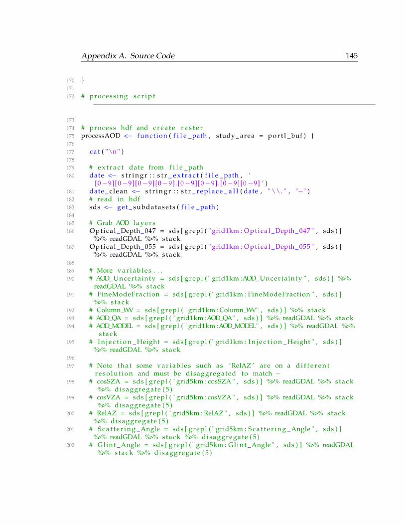
Appendix A. Source Code 145
170 }171172 # process ing s c r i p t
−−−−−−−−−−−−−−−−−−−−−−−−−−−−−−−−−−−−−−−−−−−−−−−−−−−−−−−−−−−−−−−−−−−−−−−
173174 # process hdf and c r e a t e r a s t e r175 processAOD <− func t ion ( f i l e _path , study _ area = p o r t l _ buf ) {176177 c a t ( "\n" )178179 # e x t r a c t date from f i l e _ path180 date <− s t r i n g r : : s t r _ e x t r a c t ( f i l e _path , ’
[0 −9][0 −9][0 −9][0 −9].[0 −9][0 −9].[0 −9][0 −9] ’ )181 date _ c lean <− s t r i n g r : : s t r _ r e p l a c e _ a l l ( date , " \\. " , "−" )182 # read in hdf183 sds <− get _ subdatase ts ( f i l e _ path )184185 # Grab AOD l a y e r s186 Optica l _Depth_047 = sds [ grepl ( " grid1km : Opt ica l _Depth_047 " , sds ) ]
%>% readGDAL %>% stack187 Optica l _Depth_055 = sds [ grepl ( " grid1km : Opt ica l _Depth_055 " , sds ) ]
%>% readGDAL %>% stack188189 # More v a r i a b l e s . . .190 # AOD_ Uncerta inty = sds [ grepl ( " grid1km :AOD_ Uncerta inty " , sds ) ] %>%
readGDAL %>% stack191 # FineModeFraction = sds [ grepl ( " grid1km : FineModeFraction " , sds ) ]
%>% stack192 # Column_WV = sds [ grepl ( " grid1km : Column_WV" , sds ) ] %>% stack193 # AOD_QA = sds [ grepl ( " grid1km :AOD_QA" , sds ) ] %>% readGDAL %>% stack194 # AOD_MODEL = sds [ grepl ( " grid1km :AOD_MODEL" , sds ) ] %>% readGDAL %>%
stack195 # I n j e c t i o n _ Height = sds [ grepl ( " grid1km : I n j e c t i o n _ Height " , sds ) ]
%>% readGDAL %>% stack196197 # Note t h a t some v a r i a b l e s such as ’RelAZ ’ are on a d i f f e r e n t
r e s o l u t i o n and must be disaggregated to match −198 # cosSZA = sds [ grepl ( " grid5km : cosSZA " , sds ) ] %>% readGDAL %>% stack
%>% disaggregate ( 5 )199 # cosVZA = sds [ grepl ( " grid5km : cosVZA " , sds ) ] %>% readGDAL %>% stack
%>% disaggregate ( 5 )200 # RelAZ = sds [ grepl ( " grid5km : RelAZ " , sds ) ] %>% readGDAL %>% stack
%>% disaggregate ( 5 )201 # S c a t t e r i n g _Angle = sds [ grepl ( " grid5km : S c a t t e r i n g _Angle " , sds ) ]
%>% readGDAL %>% stack %>% disaggregate ( 5 )202 # Gl in t _Angle = sds [ grepl ( " grid5km : Gl in t _Angle " , sds ) ] %>% readGDAL
%>% stack %>% disaggregate ( 5 )
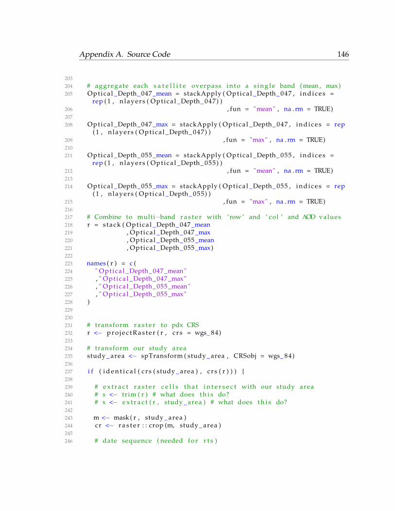
Appendix A. Source Code 146
203204 # aggregate each s a t e l l i t e overpass i n t o a s i n g l e band ( mean , max)205 Optica l _Depth_047_mean = stackApply ( Opt ica l _Depth_ 047 , i n d i c e s =
rep ( 1 , n layers ( Opt ica l _Depth_ 047) )206 , fun = "mean" , na . rm = TRUE)207208 Optica l _Depth_047_max = stackApply ( Opt ica l _Depth_ 047 , i n d i c e s = rep
( 1 , n layers ( Opt ica l _Depth_ 047) )209 , fun = "max" , na . rm = TRUE)210211 Optica l _Depth_055_mean = stackApply ( Opt ica l _Depth_ 055 , i n d i c e s =
rep ( 1 , n layers ( Opt ica l _Depth_ 055) )212 , fun = "mean" , na . rm = TRUE)213214 Optica l _Depth_055_max = stackApply ( Opt ica l _Depth_ 055 , i n d i c e s = rep
( 1 , n layers ( Opt ica l _Depth_ 055) )215 , fun = "max" , na . rm = TRUE)216217 # Combine to multi−band r a s t e r with ’row ’ and ’ col ’ and AOD values218 r = s tack ( Opt ica l _Depth_047_mean219 , Opt ica l _Depth_047_max220 , Opt ica l _Depth_055_mean221 , Opt ica l _Depth_055_max)222223 names ( r ) = c (224 " Opt ica l _Depth_047_mean"225 , " Opt ica l _Depth_047_max"226 , " Opt ica l _Depth_055_mean"227 , " Opt ica l _Depth_055_max"228 )229230231 # transform r a s t e r to pdx CRS232 r <− p r o j e c t R a s t e r ( r , c r s = wgs_ 84)233234 # transform our study area235 study _ area <− spTransform ( study _ area , CRSobj = wgs_ 84)236237 i f ( i d e n t i c a l ( c r s ( study _ area ) , c r s ( r ) ) ) {238239 # e x t r a c t r a s t e r c e l l s t h a t i n t e r s e c t with our study area240 # s <− tr im ( r ) # what does t h i s do?241 # x <− e x t r a c t ( r , study _ area ) # what does t h i s do?242243 m <− mask ( r , study _ area )244 cr <− r a s t e r : : crop (m, study _ area )245246 # date sequence ( needed f o r r t s )
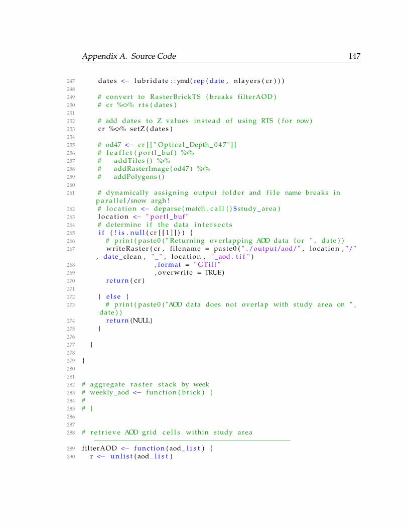
Appendix A. Source Code 147
247 dates <− l u b r i d a t e : : ymd( rep ( date , n layers ( cr ) ) )248249 # convert to RasterBr ickTS ( breaks filterAOD )250 # cr %<>% r t s ( dates )251252 # add dates to Z values ins tead of using RTS ( f o r now)253 cr %<>% setZ ( dates )254255 # od47 <− cr [ [ " Opt ica l _Depth_ 0 4 7 " ] ]256 # l e a f l e t ( p o r t l _ buf ) %>%257 # addTiles ( ) %>%258 # addRasterImage ( od47 ) %>%259 # addPolygons ( )260261 # dynamically ass igning output f o l d e r and f i l e name breaks in
p a r a l l e l /snow argh !262 # l o c a t i o n <− deparse ( match . c a l l ( ) $ study _ area )263 l o c a t i o n <− " p o r t l _ buf "264 # determine i f the data i n t e r s e c t s265 i f ( ! i s . n u l l ( c r [ [ 1 ] ] ) ) {266 # p r i n t ( paste0 ( " Returning overlapping AOD data f o r " , date ) )267 wri teRas ter ( cr , f i lename = paste0 ( " . /output/aod/" , l o c a t i o n , "/"
, date _ clean , " _ " , l o c a t i o n , " _aod . t i f " )268 , format = " GTif f "269 , overwrite = TRUE)270 re turn ( cr )271272 } e l s e {273 # p r i n t ( paste0 ( "AOD data does not overlap with study area on " ,
date ) )274 re turn (NULL)275 }276277 }278279 }280281282 # aggregate r a s t e r s tack by week283 # weekly_aod <− func t ion ( b r i c k ) {284 #285 # }286287288 # r e t r i e v e AOD grid c e l l s within study area
−−−−−−−−−−−−−−−−−−−−−−−−−−−−−−−−−−−−−−−−−−−−−−−−−289 f i l terAOD <− func t ion ( aod_ l i s t ) {290 r <− u n l i s t ( aod_ l i s t )
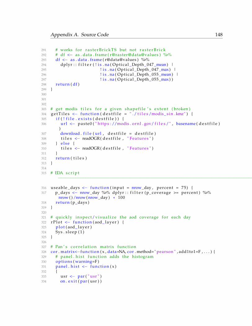
Appendix A. Source Code 148
291 # works f o r r a s t e r B r i c k T S but not r a s t e r B r i c k292 # df <− as . data . frame ( r@raster@data@values ) %>%293 df <− as . data . frame ( r@data@values ) %>%294 dplyr : : f i l t e r ( ! i s . na ( Opt ica l _Depth_047_mean) |295 ! i s . na ( Opt ica l _Depth_047_max) |296 ! i s . na ( Opt ica l _Depth_055_mean) |297 ! i s . na ( Opt ica l _Depth_055_max) )298 re turn ( df )299 }300301302303 # get modis t i l e s f o r a given s h a p e f i l e ’ s e x t e n t ( broken )304 g e t T i l e s <− func t ion ( d e s t f i l e = " . / t i l e s /modis_ s i n . kmz" ) {305 i f ( ! f i l e . e x i s t s ( d e s t f i l e ) ) {306 u r l <− paste0 ( " h t tps : //modis . ornl . gov/ f i l e s /" , basename ( d e s t f i l e )
)307 download . f i l e ( url , d e s t f i l e = d e s t f i l e )308 t i l e s <− readOGR ( d e s t f i l e , " Features " )309 } e l s e {310 t i l e s <− readOGR ( d e s t f i l e , " Features " )311 }312 re turn ( t i l e s )313 }314315 # EDA s c r i p t
−−−−−−−−−−−−−−−−−−−−−−−−−−−−−−−−−−−−−−−−−−−−−−−−−−−−−−−−−−−−−−−−−−−−−−−−−−−−−−−−
316 useable _days <− func t ion ( input = nrow_day , percent = 75) {317 p_days <− nrow_day %>% dplyr : : f i l t e r ( p_ coverage >= percent ) %>%
nrow ( ) /nrow ( nrow_day ) * 100318 re turn ( p_days )319 }320321 # quickly i n s p e c t / v i s u a l i z e the aod coverage f o r each day322 r P l o t <− func t ion ( aod_ l a y e r ) {323 p l o t ( aod_ l a y e r )324 Sys . s leep ( 1 )325 }326327 # Pan ’ s c o r r e l a t i o n matrix funct ion328 cor . matrix<−func t ion ( x , data=NA, cor . method=" pearson " , add1to1=F , . . . ) {329 # panel . h i s t funct ion adds the histogram330 options ( warning=F )331 panel . h i s t <− func t ion ( x )332 {333 usr <− par ( " usr " )334 on . e x i t ( par ( usr ) )

Appendix A. Source Code 149
335 par ( usr = c ( usr [ 1 : 2 ] , 0 , 1 . 5 ) )336 h <− h i s t ( x , p l o t = FALSE , breaks =30)337 breaks <− h$ breaks338 nB <− length ( breaks )339 y <− h$ counts340 y <− y/max( y )341 r e c t ( breaks[−nB ] , 0 , breaks [ −1] , y , c o l =" l i g h t b l u e " )342 box ( )343 }344 panel . cor <− func t ion ( x , y , d i g i t s =2 , p r e f i x =" " , cex . cor )345 {346 usr <− par ( " usr " )347 on . e x i t ( par ( usr ) )348 par ( usr = c ( 0 , 1 , 0 , 1 ) )349 r <− cor ( x , y , method=" pearson " )350 t x t <− format ( c ( r , 0 .123456789 ) , d i g i t s = d i g i t s ) [ 1 ]351 t x t <− paste ( pre f ix , t x t , sep=" " )352 i f ( missing ( cex . cor ) ) cex <− 0 . 8 /strwidth ( t x t )353 t e x t ( 0 . 5 , 0 . 5 , t x t , cex = cex * abs ( r ) )354 }355 panel . smooth2<−func t ion ( x , y , bg = NA, pch = par ( " pch " ) , cex = 1 ,
c o l . smooth = " red " , span = 2/3 , i t e r = 3 , p l o t 1 t o 1 =add1to1 )356 {357 points ( x , y , pch = pch , cex = cex , . . . )358 ok <− i s . f i n i t e ( x ) & i s . f i n i t e ( y )359 i f ( any ( ok ) ) {360 l i n e s ( s t a t s : : lowess ( x [ ok ] , y [ ok ] , f = span , i t e r = i t e r ) , c o l =
c o l . smooth )361 }362 i f ( p l o t 1 t o 1 ) {363 mn<−min ( c ( x , y ) , na . rm=T )364 mx<−max( c ( x , y ) , na . rm=T )365 new . x<−seq (mn,mx, length . out =10)366 points (new . x , new . x , type= ’ l ’ , c o l =" blue " , lwd=2)367 }368 }369 i f ( c l a s s ( x ) ==" formula " ) {370 x<−model . frame ( x , data=data )371372 }373 p a i r s ( x , upper . panel=panel . smooth2 , lower . panel=panel . cor , diag . panel=
panel . h i s t ,374 cex . l a b e l s = 1 , font . l a b e l s =2)375 options ( warning=T )376 }
Source/ggRegression.R
Appendix A. Source Code 150
1 # Define Test Regression P l o t−−−−−−−−−−−−−−−−−−−−−−−−−−−−−−−−−−−−−−−−−−−−−−−−−−−−−−−−−−−−−−−
23 scaleFUN <− func t ion ( x ) s p r i n t f ( " %.2 f " , x )45 # This p l o t i s used to compare t e s t observat ions and p r e d i c t i o n s from
ranger/randomForest models6 # Provide the names of x and y v e c t o r s as s t r i n g s7 t e s t R e g r e s s i o n <− func t ion ( df , x , y , outdir , reduced = F , c lean _ time )
{89 # Create lm model o b j e c t s
10 mod <− lm ( df [ [ y ] ] ~df [ [ x ] ] )11 mod_sum <− summary (mod)1213 # Compute RMSE on t e s t data versus p r e d i c t i o n s14 rmse <− s q r t (mean ( ( df [ [ y ] ] − df [ [ x ] ] ) ^2) )1516 # Create c o l o r p a l e t t e to display point dens i ty17 d = grDevices : : densCols ( df [ [ x ] ] , df [ [ y ] ] , colramp =
colorRampPalette ( rev ( rainbow ( 1 0 , end = 4/6) ) ) )1819 # Build our r e g r e s s i o n p l o t20 p <− ggplot ( df , aes _ s t r i n g ( x = x , y = y ) ) +21 # ylab ( " Predic ted PM2. 5 ( ug/m3) " ) +22 # xlab ( " Measured PM2. 5 ( ug/m3) " ) +23 xlab ( express ion ( ~Observed~PM[ 2 . 5 ] ~mu* g *m^−3) ) +24 ylab ( express ion ( ~Predic ted~PM[ 2 . 5 ] ~mu* g *m^−3) ) +25 # annotate ( " t e x t " , l a b e l = paste ( " R2 =" , round ( modr$ r . squared , 4 )
) , x = 25 , y = max( c ( cvr $x , cvr $y ) ) −10) +26 # annotate ( " t e x t " , l a b e l = paste ( " p−value =" , round ( modr$
c o e f f i c i e n t s [ 2 ] , 2 ) ) , x = 25 , y = max( c ( cvr $x , cvr $y ) ) −20) +27 # annotate ( " t e x t " , l a b e l = paste ( " Slope =" , round ( modr$
c o e f f i c i e n t s [ 2 ] , 2 ) ) , x = 25 , y = max( c ( cvr $x , cvr $y ) ) −20) +28 # annotate ( " t e x t " , l a b e l = paste ( " I n t e r c e p t =" , round ( modr$
c o e f f i c i e n t s [ 1 ] , 2 ) ) , x = 25 , y = max( c ( cvr $x , cvr $y ) ) −30) +29 geom_ point ( c o l = d , alpha = 0 . 5 ) +30 # coord _ f i x e d ( ) +31 s c a l e _x_ continuous ( l i m i t s = c ( min ( c ( df [ [ x ] ] , df [ [ y ] ] ) ) , max( c ( df [ [
x ] ] , df [ [ y ] ] ) ) ) ) +32 s c a l e _y_ continuous ( l i m i t s = c ( min ( c ( df [ [ x ] ] , df [ [ y ] ] ) ) , max( c ( df [ [
x ] ] , df [ [ y ] ] ) ) ) ) +33 # s c a l e _x_ continuous ( l i m i t s = c ( 0 , max( c ( cvr $x , cvr $y ) ) ) ) +34 # s c a l e _y_ continuous ( l i m i t s = c ( 0 , max( c ( cvr $x , cvr $y ) ) ) ) +35 l a b s ( s u b t i t l e = paste ( " Adj R2 = " , s i g n i f (mod_sum$ adj . r . squared ,
4 ) ,36 " I n t e r c e p t =" , s i g n i f (mod_sum$ coef [ [ 1 ] ] , 2 )
,
Appendix A. Source Code 151
37 " Slope =" , s i g n i f (mod_sum$ coef [ [ 2 ] ] , 2 ) ,38 " p =" , s i g n i f ( as . numeric ( broom : : glance (
mod) $p . value ) , 3 ) ,39 " RMSE =" , s i g n i f ( rmse , 3 ) ) ) +40 # geom_smooth ( se=F , method = " lm " , c o l = " f i r e b r i c k " ) +41 geom_ a b l i n e ( i n t e r c e p t = mod$ coef [ [ 1 ] ]42 , s lope = mod$ coef [ [ 2 ] ]43 , c o l o r = " f i r e b r i c k " ) +44 geom_ a b l i n e ( i n t e r c e p t = 045 , s lope = 146 , c o l o r = " black "47 , l i n e t y p e = " dashed "48 ) +49 theme_bw( ) +50 theme ( aspect . r a t i o = 151 , p l o t . t i t l e = element _ t e x t ( h j u s t = 0 . 5 , s i z e =12 , f a c e = "
bold " )52 , p l o t . s u b t i t l e = element _ t e x t ( h j u s t = 0 . 5 , s i z e =12 , f a c e =
" bold " )53 , a x i s . t e x t = element _ t e x t ( s i z e = r e l ( 1 . 1 ) , f a c e = " bold " ,
colour = " black " )54 , a x i s . t i t l e = element _ t e x t ( s i z e =15)55 )5657 # Assign f i l e name f o r f u l l /reduced RF model58 i f ( reduced ) {59 o u t f i l e <− paste0 ( outdir , c lean _time , "−obs−pred−lm−reduced . png " )60 } e l s e {61 o u t f i l e <− paste0 ( outdir , c lean _time , "−obs−pred−lm . png " )62 }63 p r i n t ( paste0 ( " Saving p l o t to " , o u t f i l e ) )64 ggsave ( p l o t = p65 , f i lename = o u t f i l e66 , width = 867 , he ight = 868 , u n i t s = " in "69 )70 re turn ( p )7172 }737475 # −−−−−−−−−−−−−−−−−−−−−−−−−−−−−−−−−−−−7677 # Same funct ion as above , but adds a date to the t i t l e78 dai lyRegress ion <− func t ion ( df , x , y , outdir , reduced = F , date ) {7980 # Create lm model o b j e c t s
Appendix A. Source Code 152
81 mod <− lm ( df [ [ y ] ] ~df [ [ x ] ] )82 mod_sum <− summary (mod)8384 # Compute RMSE on t e s t data versus p r e d i c t i o n s85 rmse <− s q r t (mean ( ( df [ [ y ] ] − df [ [ x ] ] ) ^2) )8687 # Create c o l o r p a l e t t e to display point dens i ty88 # d = grDevices : : densCols ( df [ [ x ] ] , df [ [ y ] ] , colramp =
colorRampPalette ( rev ( rainbow ( 1 0 , end = 4/6) ) ) )8990 # Build our r e g r e s s i o n p l o t91 p <− ggplot ( df , aes _ s t r i n g ( x = x , y = y ) ) +92 # ylab ( " Predic ted PM2. 5 ( ug/m3) " ) +93 # xlab ( " Measured PM2. 5 ( ug/m3) " ) +94 xlab ( express ion ( ~Observed~PM[ 2 . 5 ] ~mu* g *m^−3) ) +95 ylab ( express ion ( ~Predic ted~PM[ 2 . 5 ] ~mu* g *m^−3) ) +96 # annotate ( " t e x t " , l a b e l = paste ( " R2 =" , round ( modr$ r . squared , 4 )
) , x = 25 , y = max( c ( cvr $x , cvr $y ) ) −10) +97 # annotate ( " t e x t " , l a b e l = paste ( " p−value =" , round ( modr$
c o e f f i c i e n t s [ 2 ] , 2 ) ) , x = 25 , y = max( c ( cvr $x , cvr $y ) ) −20) +98 # annotate ( " t e x t " , l a b e l = paste ( " Slope =" , round ( modr$
c o e f f i c i e n t s [ 2 ] , 2 ) ) , x = 25 , y = max( c ( cvr $x , cvr $y ) ) −20) +99 # annotate ( " t e x t " , l a b e l = paste ( " I n t e r c e p t =" , round ( modr$
c o e f f i c i e n t s [ 1 ] , 2 ) ) , x = 25 , y = max( c ( cvr $x , cvr $y ) ) −30) +100 # geom_ point ( c o l = d , alpha = 0 . 5 ) +101 # geom_smooth ( se=F , method = " lm " , c o l = " f i r e b r i c k " ) +102 geom_ a b l i n e ( i n t e r c e p t = mod$ coef [ [ 1 ] ]103 , s lope = mod$ coef [ [ 2 ] ]104 , c o l o r = " f i r e b r i c k " ) +105 geom_ a b l i n e ( i n t e r c e p t = 0106 , s lope = 1107 , c o l o r = " black "108 , l i n e t y p e = " dashed "109 ) +110 geom_ point ( alpha = 0 . 5 ) +111 geom_ t e x t _ r ep e l ( point . padding = 0 . 3 0 , aes ( l a b e l = s p r i n t f ( ’ %.2 f ’ ,
s i g n i f ( df [ [ y ] ] − df [ [ x ] ] , 2 ) ) ) ) +112 # coord _ f i x e d ( ) +113 s c a l e _x_ continuous ( l a b e l s = scaleFUN , l i m i t s = c ( min ( c ( df [ [ x ] ] , df
[ [ y ] ] ) ) , max( c ( df [ [ x ] ] , df [ [ y ] ] ) ) ) ) +114 s c a l e _y_ continuous ( l a b e l s = scaleFUN , l i m i t s = c ( min ( c ( df [ [ x ] ] , df
[ [ y ] ] ) ) , max( c ( df [ [ x ] ] , df [ [ y ] ] ) ) ) ) +115 # s c a l e _x_ continuous ( l i m i t s = c ( 0 , max( c ( cvr $x , cvr $y ) ) ) ) +116 # s c a l e _y_ continuous ( l i m i t s = c ( 0 , max( c ( cvr $x , cvr $y ) ) ) ) +117 l a b s ( capt ion = paste0 ( date ) ,118 s u b t i t l e = paste ( " Adj R2 = " , s p r i n t f ( ’ %.4 f ’ , s i g n i f (mod_sum
$ adj . r . squared , 4 ) ) ,
Appendix A. Source Code 153
119 " I n t e r c e p t =" , s p r i n t f ( ’ %.2 f ’ , s i g n i f (mod_sum$ coef [ [ 1 ] ] , 2 ) ) ,
120 " Slope =" , s p r i n t f ( ’ %.2 f ’ , s i g n i f (mod_sum$coef [ [ 2 ] ] , 2 ) ) ,
121 " p =" , s p r i n t f ( ’ %.3 f ’ , s i g n i f ( as . numeric (broom : : glance (mod) $p . value ) , 3 ) ) ,
122 " RMSE =" , s p r i n t f ( ’ %.3 f ’ , s i g n i f ( rmse , 3 ) )) ) +
123 theme_bw( ) +124 theme ( aspect . r a t i o = 1125 , p l o t . t i t l e = element _ t e x t ( h j u s t = 0 . 5 , s i z e =12 , f a c e = "
bold " )126 , p l o t . s u b t i t l e = element _ t e x t ( h j u s t = 0 . 5 , s i z e =12 , f a c e =
" bold " )127 , a x i s . t e x t = element _ t e x t ( s i z e = r e l ( 1 . 1 ) , f a c e = " bold " ,
colour = " black " )128 , a x i s . t i t l e = element _ t e x t ( s i z e =15)129 )130131 # Assign f i l e name f o r f u l l /reduced RF model132 i f ( reduced ) {133 o u t f i l e <− paste0 ( outdir , s t r _ r e p l a c e _ a l l ( date , " \\. " , "−" ) , "−
obs−pred−lm−reduced . png " )134 } e l s e {135 o u t f i l e <− paste0 ( outdir , s t r _ r e p l a c e _ a l l ( date , " \\. " , "−" ) , "−
obs−pred−lm . png " )136 }137 p r i n t ( paste0 ( " Saving p l o t to " , o u t f i l e ) )138 ggsave ( p l o t = p139 , f i lename = o u t f i l e140 , width = 8141 , he ight = 8142 , u n i t s = " in "143 )144 re turn ( p )145146 }147148 # Same funct ion but with d i f f e r e n t l a b e l s −−−−−−−−−−−−−−−−−−−149 nephRegression <− func t ion ( df , x , y , outdir , reduced = F , c lean _ time )
{150151 # Create lm model o b j e c t s152 mod <− lm ( df [ [ y ] ] ~df [ [ x ] ] )153 mod_sum <− summary (mod)154155 # Compute RMSE on t e s t data versus p r e d i c t i o n s156 # rmse <− s q r t (mean ( ( df [ [ y ] ] − df [ [ x ] ] ) ^2) ) # 1 : 1 RMSE
Appendix A. Source Code 154
157 rmse <− glance (mod) $sigma # Model RMSE158 # Create c o l o r p a l e t t e to display point dens i ty159 d = grDevices : : densCols ( df [ [ x ] ] , df [ [ y ] ] , colramp =
colorRampPalette ( rev ( rainbow ( 1 0 , end = 4/6) ) ) )160161 # Build our r e g r e s s i o n p l o t162 p <− ggplot ( df , aes _ s t r i n g ( x = x , y = y ) ) +163 # ylab ( " Predic ted PM2. 5 ( ug/m3) " ) +164 # xlab ( " Measured PM2. 5 ( ug/m3) " ) +165 xlab ( express ion ( ~PurpleAir~PM[ 2 . 5 ] ~mu* g *m^−3) ) +166 ylab ( express ion ( ~Nephelometer~PM[ 2 . 5 ] ~mu* g *m^−3) ) +167 # annotate ( " t e x t " , l a b e l = paste ( " R2 =" , round ( modr$ r . squared , 4 )
) , x = 25 , y = max( c ( cvr $x , cvr $y ) ) −10) +168 # annotate ( " t e x t " , l a b e l = paste ( " p−value =" , round ( modr$
c o e f f i c i e n t s [ 2 ] , 2 ) ) , x = 25 , y = max( c ( cvr $x , cvr $y ) ) −20) +169 # annotate ( " t e x t " , l a b e l = paste ( " Slope =" , round ( modr$
c o e f f i c i e n t s [ 2 ] , 2 ) ) , x = 25 , y = max( c ( cvr $x , cvr $y ) ) −20) +170 # annotate ( " t e x t " , l a b e l = paste ( " I n t e r c e p t =" , round ( modr$
c o e f f i c i e n t s [ 1 ] , 2 ) ) , x = 25 , y = max( c ( cvr $x , cvr $y ) ) −30) +171 geom_ point ( c o l = d , alpha = 0 . 5 ) +172 # coord _ f i x e d ( ) +173 s c a l e _x_ continuous ( l i m i t s = c ( min ( c ( df [ [ x ] ] , df [ [ y ] ] ) ) , max( c ( df [ [
x ] ] , df [ [ y ] ] ) ) ) ) +174 s c a l e _y_ continuous ( l i m i t s = c ( min ( c ( df [ [ x ] ] , df [ [ y ] ] ) ) , max( c ( df [ [
x ] ] , df [ [ y ] ] ) ) ) ) +175 # s c a l e _x_ continuous ( l i m i t s = c ( 0 , max( c ( cvr $x , cvr $y ) ) ) ) +176 # s c a l e _y_ continuous ( l i m i t s = c ( 0 , max( c ( cvr $x , cvr $y ) ) ) ) +177 l a b s ( s u b t i t l e = paste ( "R2 = " , s i g n i f (mod_sum$ adj . r . squared , 4 ) ,178 " I n t e r c e p t =" , s i g n i f (mod_sum$ coef [ [ 1 ] ] , 2 ) ,179 " Slope =" , s i g n i f (mod_sum$ coef [ [ 2 ] ] , 2 ) ,180 " p =" , s i g n i f ( as . numeric ( broom : : glance (mod
) $p . value ) , 3 ) ,181 " RMSE =" , s i g n i f ( rmse , 3 ) ) ) +182 # geom_smooth ( se=F , method = " lm " , c o l = " f i r e b r i c k " ) +183 geom_ a b l i n e ( i n t e r c e p t = mod$ coef [ [ 1 ] ]184 , s lope = mod$ coef [ [ 2 ] ]185 , c o l o r = " f i r e b r i c k " ) +186 geom_ a b l i n e ( i n t e r c e p t = 0187 , s lope = 1188 , c o l o r = " black "189 , l i n e t y p e = " dashed "190 ) +191 theme_bw( ) +192 theme ( aspect . r a t i o = 1193 , p l o t . t i t l e = element _ t e x t ( h j u s t = 0 . 5 , s i z e =12 , f a c e = "
bold " )194 , p l o t . s u b t i t l e = element _ t e x t ( h j u s t = 0 . 5 , s i z e =12 , f a c e =
" bold " )
Appendix A. Source Code 155
195 , a x i s . t e x t = element _ t e x t ( s i z e = r e l ( 1 . 1 ) , f a c e = " bold " ,colour = " black " )
196 , a x i s . t i t l e = element _ t e x t ( s i z e =15)197 )198199 o u t f i l e <− paste0 ( outdir , c lean _time , "−obs−pred−lm . png " )200201 # Assign f i l e name f o r f u l l /reduced RF model202 i f ( reduced ) {203 o u t f i l e <− paste0 ( outdir , c lean _time , " _obs_pred−lm−reduced . png " )204 } e l s e {205 o u t f i l e <− paste0 ( outdir , c lean _time , "−obs−pred−lm . png " )206 }207208 p r i n t ( paste0 ( " Saving p l o t to " , o u t f i l e ) )209 ggsave ( p l o t = p210 , f i lename = o u t f i l e211 , width = 8212 , he ight = 8213 , u n i t s = " in "214 )215 re turn ( p )216217 }
Source/homogeneousPM.R1 # crea ted by P h i l i p Orlando @ S u s t a i n a b l e Atmopsheres Research Lab2 # Canopy Continuum P r o j e c t , USFS3 # PI Dr . Linda George4 # 2018−09−175 # e x t r a c t r e g i o n a l l y homogenous neph PM (+/− 10% of network mean)67 # s e t up environment
−−−−−−−−−−−−−−−−−−−−−−−−−−−−−−−−−−−−−−−−−−−−−−−−−−−−−−−−−−−−−−−89 # load the necessary packages
10 i f ( ! r equi re ( pacman ) ) {11 i n s t a l l . packages ( " pacman " )12 l i b r a r y ( pacman )13 }1415 p_ load ( readr16 , readxl17 # , x l s x18 , ggplot219 , r a s t e r20 , p lyr
Appendix A. Source Code 156
21 , dplyr22 # , mult idplyr23 , broom24 , reshape225 , t i d y r26 , s t r i n g r27 , ma gr i t t r28 , r l i s t29 , gr id30 , g r idExtra31 , t idyquant32 , s c a l e s33 , qdapRegex34 , sp35 , s f36 # ,mapview # * * * * * with s p e c i f i c l e a f l e t i n s t a l l37 , devtools38 , RColorBrewer39 , c l a s s I n t40 , h tml tools41 , s c a l e s42 , htmlwidgets43 , h t t r44 , j s o n l i t e45 , rgdal46 , pbapply47 , snow48 , p a r a l l e l49 , data . t a b l e50 , RPostgres51 , t s o u t l i e r s52 , f o r e c a s t53 ,MASS54 , v i r i d i s55 , c o r r p l o t56 , nngeo57 )5859 # def ine g loba l v a r i a b l e s
−−−−−−−−−−−−−−−−−−−−−−−−−−−−−−−−−−−−−−−−−−−−−−−−−−−−−−−−−−−−−−−−−−−
60 source ( " . / s r c /ggRegression . R" )61 source ( " . / s r c / i n i t . R" )6263 # s e t timezone to UTC/GMT to match postgres64 # otherwise , s t _ read ( ) w i l l convert timestamp to US/ P a c i f i c with PST/
PDT!65 # DEQ only uses PST !
Appendix A. Source Code 157
66 Sys . timezone ( )67 Sys . setenv (TZ="GMT" )68 Sys . timezone ( )6970 ## connect ing to l o c a l db71 host <− ’ pgsql120 . rc . pdx . edu ’72 db <− ’ canopycontinuum ’73 user <− ’ porlando ’74 port <− 543375 pw <− scan ( " . / b a t t e r i e s . pgpss " , what = " " ) # in parent d i r767778 # open connect ion to our db79 con <− dbConnect ( drv = RPostgres : : Postgres ( )80 ,dbname = db81 , host = ’ pgsql102 . rc . pdx . edu ’ # not sure why o b j e c t
host isn ’ t working . . .82 , port = port83 , password = pw84 , user = user )8586 # c r e a t e unanimous time r e s o l u t i o n f o r a l l data87 time _ r e s o l u t i o n <− " 1 sec "8889 # time zone applied to a l l data90 time _zone <− "GMT"9192 # CRS93 wgs_84 <− "+pro j= l o n g l a t + e l l p s =WGS84 +datum=WGS84 +no_ defs "9495 # Oregon North NAD83 HARN meters96 epsg_ 2838 <− "+pro j= l c c + l a t _1=46 + l a t _ 2=44.33333333333334 + l a t _
0=43.66666666666666 +lon _0=−120.5 +x_ 0=2500000 +y_0=0 + e l l p s =GRS80+ u n i t s =m +no_ defs "
9798 # Oregon North NAD83 Meters UTM Zone 1099 epsg_ 26910 <− "+pro j=utm +zone=10 + e l l p s =GRS80 +datum=NAD83 + u n i t s =m
+no_ defs "100101 # Function d e f i n i t i o n
−−−−−−−−−−−−−−−−−−−−−−−−−−−−−−−−−−−−−−−−−−−−−−−−−−−−−−−−−−−−−−−−−−102103 # c r e a t i n g a custon not−in funct ion104 ’%! in%’ <− func t ion ( x , y ) ! ( ’%in%’ ( x , y ) )105106 # p l o t dens i ty in ggplot107 get _ densi ty <− func t ion ( x , y , n = 100) {108 dens <− MASS : : kde2d ( x = x , y = y , n = n )
Appendix A. Source Code 158
109 i x <− f i n d I n t e r v a l ( x , dens$x )110 iy <− f i n d I n t e r v a l ( y , dens$y )111 i i <− cbind ( ix , iy )112 re turn ( dens$z [ i i ] )113 }114115 s e t . seed ( 1 )116117 # data process ing
−−−−−−−−−−−−−−−−−−−−−−−−−−−−−−−−−−−−−−−−−−−−−−−−−−−−−−−−−−−−−−−−−−−−−−−−−
118 # s t a r t _ date <− "2017−07−01"119 # end_ date <− "2018−09−30"120 # i n h e r i t s t a r t /end date from i n i t s c r i p t in modeling p r o j e c t121122 # t h i s should work once I update my pdx t a b l e123 # pa <− s t _ read ( dsn = con124 # # ,geom_column = "geom" # depreceated !125 # # ,EWKB = TRUE126 # , query = paste0 ( " SELECT DISTINCT * FROM pdx WHERE
created _ a t >= ’ "127 # , l u b r i d a t e : : ymd( s t a r t _ date ) + hours
( 8 )128 # , " ’ AND created _ a t <= ’ "129 # , l u b r i d a t e : : ymd( end_ date ) + hours ( 8 ) ,
" ’ ; " )130 # )131 # saveRDS ( pa , " . /data/frm/purpleAir5min . RDS" )132 # pa <− readRDS ( " . /data/frm/purpleAir5min . RDS" )133134 # hourly group by with s q l
−−−−−−−−−−−−−−−−−−−−−−−−−−−−−−−−−−−−−−−−−−−−−−−−−−−−−−−−−−−−−−−−−135 pa <− s t _ read ( dsn = con136 # ,geom_column = "geom" # depreceated !137 # ,EWKB = TRUE138 , query = paste0 ( "SELECT date ( a . c rea ted _ at ) , date _ part ( ’
hour ’ , a . c rea ted _ a t ) as hour , a . id , a . sensor , a . l a b e l , avg ( a . pm2_5_atm ) pm2_5_atm , a . geom
139 FROM (SELECT DISTINCT * FROM pdx WHEREcreated _ a t >= ’ "
140 , l u b r i d a t e : : ymd( s t a r t _ date ) + hours ( 8 )141 , " ’ AND created _ a t <= ’ "142 , l u b r i d a t e : : ymd( end_ date ) + hours ( 8 ) , "
’ ) a143 GROUP BY a . id , a . sensor , a . l a b e l , a .
geom , date ( a . c rea ted _ at ) , date _ part ( ’ hour ’ , a . c rea ted _ at ) ; " )144 )145

Appendix A. Source Code 159
146 pa$ crea ted _ at <− paste ( pa$ date , pa$hour )147 pa$ crea ted _ at <− ymd_h ( pa$ created _ a t )148 pa$ crea ted _ at <− pa$ crea ted _ at − hours ( 8 )149 pa %<>% dplyr : : s e l e c t ( c rea ted _ at , everything ( ) , −c ( date , hour ) )150 names ( pa ) [ names ( pa ) == " crea ted _ a t " ] <− " datetime "151152 # 15 minute average PurpleAir
−−−−−−−−−−−−−−−−−−−−−−−−−−−−−−−−−−−−−−−−153 # hourly group by with s q l154 pa <− s t _ read ( dsn = con155 # ,geom_column = "geom" # depreceated !156 # ,EWKB = TRUE157 , query = paste0 ( "SELECT date _ trunc ( ’ hour ’ , a . c rea ted _ at
) + date _ part ( ’ minute ’ , a . c rea ted _ at ) : : i n t / 15 * i n t e r v a l ’15 min’ AS created _ at
158 , a . id , a . sensor , a . l a b e l , avg ( a . pm2_5_atm ) pm2_5_atm , a . geom
159 FROM (SELECT DISTINCT * FROM pdx WHEREcreated _ a t >= ’ "
160 , l u b r i d a t e : : ymd( s t a r t _ date ) + hours ( 8 )161 , " ’ AND created _ a t <= ’ "162 , l u b r i d a t e : : ymd( end_ date ) + hours ( 8 ) , "
’ ) a163 GROUP BY a . id , a . sensor , a . l a b e l , a .
geom164 , date _ trunc ( ’ hour ’ , a . c rea ted _ at ) +
date _ part ( ’ minute ’ , a . c rea ted _ a t ) : : i n t / 15 * i n t e r v a l ’15 min ’ ; " )165 )166167 #### pa$ crea ted _ at <− paste ( pa$ date , pa$hour , pa$ f i f t e e n )168 pa$ crea ted _ at <− ymd_hms( pa$ created _ a t )169 pa$ crea ted _ at <− pa$ crea ted _ at − hours ( 8 )170 pa %<>% dplyr : : s e l e c t ( c rea ted _ at , everything ( ) )171 # make sure the datetime columns match172 names ( pa ) [ names ( pa ) == " crea ted _ a t " ] <− " datetime "173174 # End 15−minute read PA
−−−−−−−−−−−−−−−−−−−−−−−−−−−−−−−−−−−−−−−−−−−−−−−−−−−−−−−−−175176 # lookup t a b l e f o r sensor geom177 pa_ points <− s t _ read ( dsn = con178 # ,geom_column = "geom"179 # ,EWKB = TRUE180 # , query = "SELECT DISTINCT * FROM pdx_ l o c a l _
s lope ; "181 # , query = "SELECT DISTINCT * FROM pdx ; "182 # compare PurpleAir to DEQ during r e g i o n a l PM
event ( w i l d f i r e )
Appendix A. Source Code 160
183 , query = "SELECT DISTINCT id , l a b e l , geom FROMpdx GROUP BY id , l a b e l , geom ; "
184 )185186 # def ine p r o j e c t i o n187 s t _ c r s ( pa ) <− epsg_ 26910188 # s t _ c r s ( pa_ hourly ) <− epsg_ 26910189 s t _ c r s ( pa_ points ) <− epsg_ 26910190191 # R e l a t i v e standard devia t ion c a l c
−−−−−−−−−−−−−−−−−−−−−−−−−−−−−−−−−−−−−−−−−−−−−−−−−−−−−−−−−−−−−−−−−−−−−−−−−−−−
192 # Reading in 5−minute neph data193 # neph <− readRDS ( " . /data/deq/neph5min . RDS" )194 frm <− readRDS ( " . /data/deq/neph5min . RDS" )195 # frm <− readRDS ( " . /data/deq/neph1hour . RDS" )196197 rsd <− func t ion ( sd , mean) {198 sd/mean199 }200201 # 15−minute only −−−−−−−−−−−−−−−−−−−−−−−−−−−−−−−−−−−−−−−−−−−−−−−−−202 # Group by 15−minute c lean breaks !203 frm$ datetime <− f l o o r _ date ( frm$ datetime , " 15 minutes " )204205 frm %<>% dplyr : : s e l e c t (−date ) %>% s t _drop_geometry ( ) %>%206 group_by ( datetime , s i t e _ id ) %>% summarise (pm2_5_ r e f = mean(pm2_5_
r e f ) )207 # 15−minute only −−−−−−−−−−−−−−−−−−−−−−−−−−−−−−−−−−−−−−−−−−−−−−−−−208209 # aggregate by 15 minutes ( or 1 hour )210 frm_mean <− frm %>% group_by ( datetime ) %>% summarise (pm2_5_mean =
mean(pm2_5_ r e f )211 , n_mean = n ( )212 ,pm2_5_ rsd = rsd
( sd (pm2_5_ r e f ) , mean(pm2_5_ r e f ) ) )213214 # Reduce minimum s i t e s to 4 (2017 data missing 1 s i t e ? Cully )215 rsd _ threshold <− 0 . 1 0216 # n_min <− 4 # 1−hour217 n_min <− 5 # 15−min218 time _ r es <− "15−min "219220 # For 1−hour data221 # frm_mean %>% f i l t e r (pm2_5_ rsd <= 0 . 1 0 ) %>% f i l t e r ( n_mean >= n_min &
n_mean <= 6) %>% s t _drop_geometry ( ) %>% nrow ( )222 # frm_mean %<>% f i l t e r (pm2_5_ rsd <= 0 . 0 5 ) %>% f i l t e r ( n_mean >= n_min
& n_mean <= 6) %>% s t _drop_geometry ( )
Appendix A. Source Code 161
223224 # For 15−minute data225 frm_mean %>% f i l t e r (pm2_5_ rsd <= rsd _ threshold ) %>% f i l t e r ( n_mean >=
n_min & n_mean <= 6) %>% s t _drop_geometry ( ) %>% nrow ( )226 frm_mean %<>% f i l t e r (pm2_5_ rsd <= rsd _ threshold ) %>% f i l t e r ( n_mean >=
n_min & n_mean <= 6) %>% s t _drop_geometry ( )227228229 # Calc percent d i f f e r e n c e
−−−−−−−−−−−−−−−−−−−−−−−−−−−−−−−−−−−−−−−−−−−−−−−−−−−−−−−−−−−−−−−−−−−−−−−−−−−−−−−−−−−−−
230 # frm %<>% inner _ j o i n ( frm_mean)231 # summary ( frm )232 #233 # # DEQ 24−h datetime i s introducing d u p l i c a t e s around midnight ?234 # frm$hour <− hour ( frm$ datetime )235 # frm %<>% f i l t e r ( hour ! = 0)236 # frm %<>% f i l t e r ( n_mean >=4 & n_mean <=6)237 #238 # # percent d i f f e r e n c e funct ion239 # pct _ d i f f <− func t ion ( v1 , v2 ) {240 # abs ( v1−v2 ) / ( ( v1+v2 ) /2)241 # }242 #243 # # Find hours with low v a r i a t i o n among 5−6 nephelometers244 # frm$ pct _ d i f f <− pct _ d i f f ( frm$pm2_5_ ref , frm$pm2_5_mean)245 #246 # frm_homo <− frm %>% f i l t e r ( pct _ d i f f <= 0 . 1 0 ) %>% arrange ( datetime )247 #248 # # J o i n mean pct d i f f with mean pm by datetime249 # frm_mean_homo <− frm_homo %>% group_by ( datetime ) %>%250 # summarise ( pct _ d i f f _mean = mean( pct _ d i f f ) , n_ pct = n ( ) ) %>% f i l t e r
( n_ pct >= 5) %>% l e f t _ j o i n ( frm_mean)251 #252 # # J o i n mean pct d i f f with mean pm by datetime and by s i t e id !253 # frm_ s i t e _homo <− frm_homo %>% group_by ( datetime ) %>%254 # summarise ( pct _ d i f f _mean = mean( pct _ d i f f ) , n_ pct = n ( ) ) %>% f i l t e r
( n_ pct >= 5) %>% l e f t _ j o i n ( frm )255 #256 # frm %<>% s t _ as _ s f ( coords = c ( " lon " , " l a t " ) , c r s = wgs_ 84)257 # frm <− frm_mean_homo # mean % d i f f e r e n c e of mean258 frm <− frm_mean # RSD259260 # J o i n DEQ with PA
−−−−−−−−−−−−−−−−−−−−−−−−−−−−−−−−−−−−−−−−−−−−−−−−−−−−−−−−−−−−−−−−−−−−−−−−−−−−−−−−−−−−−−−−−−−−
261 # matching the s e l f i l e with the 5 stn id
Appendix A. Source Code 162
262 # frm$ s i t e _ id <− i f e l s e ( frm$ s i t e _ id == "PM2 5L_ Est " , " Port land SEL a f a y e t t e " , frm$ s i t e _ id )
263 s t r ( frm )264 s t r ( pa )265 # s t r ( pa_ hourly )266267 # check the time zone of pa data268 a t t r ( pa$ datetime , " tzone " )269 # a t t r ( pa_ hourly $ datetime , " tzone " )270 a t t r ( frm$ datetime , " tzone " )271272 # Convert DEQ data to UTC!273 # frm$ datetime <− with_ tz ( frm$ datetime , tzone = "UTC" )274 # a t t r ( frm$ datetime , " tzone " )275276 # DEQ datetime isn ’ t in US/ P a c i f i c , i t ’ s UTC−8 ( they don ’ t observe
DST)277 # Convert tz without changing datetime278 # pa$ datetime <− f o r c e _ tz ( pa$ datetime , "US/ P a c i f i c " )279 # pa$ datetime <− f o r c e _ tz ( pa$ datetime , "GMT" )280 a t t r ( pa$ datetime , " tzone " )281282 # pa_ hourly $ datetime <− f o r c e _ tz ( pa_ hourly $ datetime , "US/ P a c i f i c " )283 # a t t r ( pa_ hourly $ datetime , " tzone " )284285286 # J o i n mean neph data with PA
−−−−−−−−−−−−−−−−−−−−−−−−−−−−−−−−−−−−−−−−−−−−−−−−−−−−−−−−−−−−−287 df <− inner _ j o i n ( pa , frm )288 # df <− inner _ j o i n ( pa_ hourly , frm )289 df $ year <− l u b r i d a t e : : year ( df $ datetime )290 df $month <− l u b r i d a t e : : month ( df $ datetime , l a b e l = TRUE)291292 # Exclude o u t l i e r s in PurpleAir and Neph293 df %<>% f i l t e r (pm2_5_atm <= max_pm_ range ) # g loba l v a r i a b l e s tored in
i n i t . R294 saveRDS ( df , paste0 ( " . /data/homogenousPM/df _ " , time _ res , " . RDS" ) )295296 # Loop through each sensor and run r e g r e s s i o n297 sensors <− unique ( df $ id ) # use id here ins tead of l a b e l b/c i t has
d u p l i c a t e s ( e . g . M i l l e r )298 system ( "rm . / f i g u r e s /pa_neph_ c a l /*/* . png " )299300 r _ squared _ threshold <− 0 . 9 0301 n_obs_ threshold <− 50302303 lm_ r e s u l t s <− Reduce ( rbind , pblapply ( sensors , funct ion ( n ) {304

Appendix A. Source Code 163
305 # S e l e c t s p e c i f i c node306 df _ sensor <− f i l t e r ( df , id %in% n )307 l a b e l <− df _ sensor $ l a b e l [ 1 ] %>% gsub ( pat te rn = "\\s|\\/|\\. " ,
replacement = " _ " ) %>% tolower ( )308309 # Run models −−−−−−−−−−−−−−−−−−−−−−−−−310 mod <− lm (pm2_5_mean~pm2_5_atm , df _ sensor )311 summary_lm <− broom : : glance (mod)312 summary_lm$ slope <− mod$ coef [ [ 2 ] ]313 summary_lm$ i n t e r c e p t <− mod$ coef [ [ 1 ] ]314 # summary_lm$model_ type <− " lm"315 summary_lm$n_obs <− nrow ( df _ sensor )316 summary_lm$ id <− n317318 # V i s u a l i z e CV −−−−−−−−−−−−−−−−−−−−−−−−−−−−−−319 t r y ( {320321 i f ( summary_lm$ r . squared >= r _ squared _ threshold & summary_lm$n_obs
>= n_obs_ threshold ) {322 nephRegression ( df = df _ sensor , y = "pm2_5_mean" , x = "pm2_5_atm
" , outdir = " . / f i g u r e s /pa_neph_ c a l /pass/"323 , c lean _ time = paste0 ( " lm_ " , l a b e l ) , reduced = F )324 } e l s e {325 nephRegression ( df = df _ sensor , y = "pm2_5_mean" , x = "pm2_5_atm
" , outdir = " . / f i g u r e s /pa_neph_ c a l / f a i l /"326 , c lean _ time = paste0 ( " lm_ " , l a b e l ) , reduced = F )327 }328 } )329330 re turn ( summary_lm )331 }332 # , c l =detectCores ( )−1333 )334 )335336 saveRDS ( lm_ r e s u l t s , paste0 ( " . /data/homogenousPM/lm_ r e s u l t s _ " , time _
res , " . RDS" ) )337 system ( paste0 ( " zip −r . / f i g u r e s /lm_ rsd10 _ " , time _ res , " . zip . / f i g u r e s
/pa_neph_ c a l " ) )338339 # see . / s r c /compareCF . R f o r 15−min vs . 1−hour comparison340341 lm_ df <− lm_ r e s u l t s %>% f i l t e r ( r . squared >= r _ squared _ threshold ) %>%342 f i l t e r ( n_obs >= n_obs_ threshold )343344 r2 _ v i o l i n <− ggplot ( lm_ r e s u l t s , aes ( x = id , y = r . squared ) ) +345 geom_ v i o l i n ( f i l l = " cornf lowerblue " ) +

Appendix A. Source Code 164
346 geom_ h l i n e ( y i n t e r c e p t = r _ squared _ threshold , c o l o r = " f i r e b r i c k " ,l i n e t y p e = 2) +
347 ylab ( express ion (R^2) ) +348 # g g t i t l e ( paste0 ( express ion ( D i s t r i b u t i o n of R^2) , " ( Nephelometer~
PurpleAir ) " ) ) +349 g g t i t l e ( bquote ( ’ D i s t r i b u t i o n of ’~R^2~ ’ ( Nephelometer~PurpleAir ) ’~ . (
time _ r es ) ) ) +350 theme_bw( ) +351 theme ( a x i s . t i t l e . x = element _ blank ( ) , a x i s . t e x t . x = element _ blank ( )
, a x i s . t i c k s . x = element _ blank ( ) )352353 r2 _ v i o l i n354355 png ( f i lename = paste0 ( " . / f i g u r e s /pa_neph_ v i o l i n s /r2 _ " , time _ res , " .
png " )356 , width = 8357 , he ight = 6358 , u n i t s = " in "359 , r e s = 300360 )361 r2 _ v i o l i n362 dev . o f f ( )363364 s lope _ v i o l i n <− ggplot ( lm_df , aes ( x = id , y = slope ) ) +365 geom_ v i o l i n ( f i l l = " f o r e s t g r e e n " ) +366 ylab ( express ion ( beta ) ) +367 g g t i t l e ( paste0 ( " D i s t r i b u t i o n of Slopes ( Nephelometer~PurpleAir ) " ,
time _ r es ) ) +368 theme_bw( ) +369 theme ( a x i s . t i t l e . x = element _ blank ( ) , a x i s . t e x t . x = element _ blank ( )
, a x i s . t i c k s . x = element _ blank ( ) )370371 s lope _ v i o l i n372373 png ( f i lename = paste0 ( " . / f i g u r e s /pa_neph_ v i o l i n s /slope _ " , time _ res , " .
png " )374 , width = 8375 , he ight = 6376 , u n i t s = " in "377 , r e s = 300378 )379 s lope _ v i o l i n380 dev . o f f ( )381382 # I ’m scrapping t h i s idea f o r now . Might r e v i s i t 15−minute CF l a t e r
i f needed . . .383 # Salvage any " f a i l e d " sensors by hand384 # id _ pass <− c ( )

Appendix A. Source Code 165
385386 # Connect CF to each PurpleAir and upload to DB
−−−−−−−−−−−−−−−−−−−−−−−−−−−−−−−−−−−−−−−−−−−−−−−−−−−−−−−−−−−−387388 # Checkpoint our homogenous PM r e s u l t s f o r our CF s c r i p t389 saveRDS ( lm_df , " . /data/ c f /homogenous_pm_ c f . RDS" )390391 # Apply bes t method from EDA to pdx_ c f392 # Do t h i s a f t e r s t o r i n g data in DB ( s t o r e even bad sensors CF f o r now
. . . )393 # pdx_ c f %<>%394 # group_by ( id , l a b e l ) %>%395 # s l i c e ( which . max( r . squared ) ) %>%396 # f i l t e r ( r . squared >= 0 . 8 0 ) %>% arrange ( l a b e l )397398 # Append geometry and convert to s i m p l e f e a t u r e s399 pdx_ c f <− inner _ j o i n ( lm_df , pa_ points ) %>% s t _ as _ s f ( )400401 # Prepare colnames f o r postgres ( remove periods )402 names ( pdx_ c f ) <− gsub ( x = names ( pdx_ c f ) , pa t te rn = " \\. " , " _ " ) %>%
tolower ( )403 # names ( pdx_ c f ) [ names ( pdx_ c f ) == " id " ] <− " l a b e l "404405 # HTMS Roof was re turning I n f and NaN406 pdx_ c f %<>% na . omit ( )407408 saveRDS ( pdx_ cf , " . /data/ c f /pdx_ c f . RDS" )409410 # open connect ion to our db411 con <− dbConnect ( drv = RPostgres : : Postgres ( )412 ,dbname = db413 , host = ’ pgsql102 . rc . pdx . edu ’ # not sure why o b j e c t
host isn ’ t working . . .414 , port = port415 , password = pw416 , user = user )417418 # Find a b e t t e r way to do t h i s . . . append = TRUE i s not idea l , but
append = FALSE and overwrite = TRUE converts numeric to r e a ldatatype ! ?
419 # Write to db as lookup t a b l e420421 # c l e a r t a b l e before wri t ing new data422 r es <− dbSendQuery ( con , statement = " d e l e t e from pdx_ c f ; " )423 dbClearResult ( re s )424 r es <− dbSendQuery ( con , statement = "vacuum f u l l pdx_ c f ; " )425 dbClearResult ( re s )426
Appendix A. Source Code 166
427 # Write the new CF data to the pdx_ c f t a b l e in canopycontinuum428 s t _ wri te ( ob j = pdx_ c f429 , dsn = con430 , l a y e r _ opt ions = "OVERWRITE=true "431 , drop_ t a b l e = FALSE432 , t r y _drop = FALSE433 , debug = TRUE434 , append = TRUE435 , overwrite = FALSE436 , d a t a s e t _ opt ions = "GEOMETRY=AS_WKT"437 )438439 # TODO c r e a t e new pdx_ c f t a b l e with appropriate a t t r i b u t e names !440 # c f <− s t _ read ( dsn = con441 # # ,geom_column = "geom"442 # # ,EWKB = TRUE443 # # , query = "SELECT DISTINCT * FROM pdx_ l o c a l _ s lope ; "444 # # , query = "SELECT DISTINCT * FROM pdx ; "445 # # compare PurpleAir to DEQ during r e g i o n a l PM event (
w i l d f i r e )446 # , query = "SELECT * FROM pdx_ c f ; "447 # )448449 # INSERT FLAG DATA SCRIPT HERE
−−−−−−−−−−−−−−−−−−−−−−−−−−−−−−−−−−−−−−−−−−−−−−−−−−−−−−−−−−−−−450 # added to processPurpleAir in aod_modeling ins tead . . .451 # pdx_ f l a g <− s t _ read ( dsn = con452 # ,geom_column = "geom"453 # , query = "SELECT DISTINCT * FROM pdx_ f l a g ; " )454 #
−−−−−−−−−−−−−−−−−−−−−−−−−−−−−−−−−−−−−−−−−−−−−−−−−−−−−−−−−−−−−−−−−−−−−−−−−−−−−−−−−−−−−−−−−−
Source/init.R1 l i b r a r y ( r a s t e r )2 l i b r a r y ( pbapply )3 source ( " . / s r c /f u n c t i o n s . R" )45 # Global Var iab le d e f i n i t i o n
−−−−−−−−−−−−−−−−−−−−−−−−−−−−−−−−−−−−−−−−−−−−−−−−−−−−−−−−−−−−−−−−−−−−−
6 # Oregon North NAD83 Meters UTM Zone 107 epsg_ 26910 <− "+pro j=utm +zone=10 + e l l p s =GRS80 +datum=NAD83 + u n i t s =m
+no_ defs "8 wgs_84 <− "+pro j= l o n g l a t + e l l p s =WGS84 +datum=WGS84 +no_ defs "9
10 # Port land Study Area

Appendix A. Source Code 167
11 study _ area <− " . /study _ area/study _ area . RDS"12 bb <− " . /study _ area/bb . RDS"1314 # Study s t a r t and end date15 s t a r t _ date = " 2017−09−01 "16 # end_ date = "2018−09−30" # note , download/processGridMET must be re−
ran i f more r e c e n t end date i s required !17 # end_ date = "2019−05−29"18 end_ date = " 2019−03−31 " # GridMet and PBL l i m i t e d to ~Apri l1920 c r s = epsg_ 2691021 study _ area = " . /study _ area/study _ area . RDS"22 pm_ df = " . /data/purplea i r/pm_ df _24h . RDS"2324 # f o r t e s t i n g f u n c t i o n s25 date <− " 2 0 1 7 . 1 0 . 1 0 "2627 # Minimun S p a t i a l Resolut ion f o r a l l v a r i a b l e s28 sp_ r es <− 50 # meters2930 # Max PM range ( used f o r portlandCF . R , and processPurpleAir . R)31 max_pm_ range <− 2503233 # Use nephelometer data as a s c a l i n g f a c t o r f o r PurpleAir network ?34 s c a l e _neph = F3536 # Set tmpdir f o r r a s t e r data37 setRasterTempDir ( )3839 # Raster black white c o l o r p a l e t t e40 bw <− colorRampPalette ( c ( ’ white ’ , ’ b lack ’ ) ) ( 5 0 )4142 # P r i n t progressbar to CL43 pbo = pboptions ( type=" t imer " )
Source/interpolateNDVI.R1 # load the necessary packages2 i f ( ! r equi re ( pacman ) ) {3 i n s t a l l . packages ( " pacman " )4 l i b r a r y ( pacman )5 }67 p_ load ( rgdal8 , r a s t e r9 , sp
10 , rgeos11 , pbapply
Appendix A. Source Code 168
12 # , r a s t e r V i s13 , zoo14 , ma gr i t t r15 , p a r a l l e l16 # , greenbrown # sourceforge repo17 )181920 # l i b r a r y ( r a s t e r ) ; l i b r a r y ( r a s t e r V i s ) ; l i b r a r y ( zoo )21 # r1 = r a s t e r ( matrix ( c (NA, rep ( 1 , 8 ) ) , 3 , 3 ) )22 # r2 = r a s t e r ( matrix ( c (NA, rep ( 2 , 8 ) ) , 3 , 3 ) )23 # r3 = r a s t e r ( matrix ( c (NA, rep ( 3 , 8 ) ) , 3 , 3 ) )24 # b1 = b r i c k ( l i s t ( r1 , r2 , r3 ) )25 # l e v e l p l o t ( b1 )26 #27 # # f i l l in empty time s teps28 # b2 = b r i c k ( lapply ( 1 : 9 , funct ion ( x ) r a s t e r ( matrix (NA, 3 , 3 ) ) ) )29 #30 # old . l a y e r s = c ( 1 , 4 , 7 )31 # f o r ( i in 1 : n layers ( b1 ) ) {32 # b2 [ [ old . l a y e r s [ i ] ] ] = b1 [ [ i ] ]33 # }34 # l e v e l p l o t ( b2 , layout=c ( 9 , 1 ) )35 #36 # f o r ( c e l l in 1 : n c e l l ( b2 ) ) {37 # i f ( a l l ( i s . na ( as . vec tor ( b2 [ c e l l ] ) ) ) ) {38 # # na . s p l i n e wil f a i l i f a l l are NA39 # new . values = as . numeric ( rep (NA, dim ( b2 ) [ 3 ] ) )40 # } e l s e {41 # new . values = na . s p l i n e ( as . vec tor ( b2 [ c e l l ] ) , na . rm = F )42 # }43 # b2 [ c e l l ] [ ] = new . values44 # }45 # l e v e l p l o t ( b2 , layout=c ( 9 , 1 ) )4647 ndvi <− s tack ( l i s t . f i l e s ( path = " . /output/ndvi/" , pa t te rn = " . t i f $ " ,
f u l l . names = T ) )48 # l e v e l p l o t ( ndvi )4950 evi <− s tack ( l i s t . f i l e s ( path = " . /output/evi/" , pa t te rn = " . t i f $ " ,
f u l l . names = T ) )51 # l e v e l p l o t ( evi )5253 # Graphica l ly a s s e s s l a y e r s with cloud i n t e r f e r e n c e54 # cloud _days <−
" 2 0 1 7 . 0 8 . 2 9 | 2 0 1 7 . 1 1 . 0 1 | 2 0 1 8 . 0 1 . 1 7 | 2 0 1 8 . 0 2 . 1 8 | 2 0 1 8 . 0 3 . 2 2 "5556 # F i l t e r out bad Landsat scenes
Appendix A. Source Code 169
57 # ndvi <− subset ( ndvi , grep ( cloud _days , names ( ndvi ) , value = T ,i n v e r t =T ) )
58 # evi <− subset ( evi , grep ( cloud _days , names ( evi ) , value = T , i n v e r t =T) )
59 # ndvi <− subset ( ndvi , grep ( " 2 0 1 7 . 0 9 . 1 4 | 2 0 1 7 . 0 9 . 3 0 " , names ( ndvi ) ,value = T , i n v e r t =F ) )
6061 getDates <− func t ion ( s tack ) {62 names <− names ( s tack )63 dates <− gsub ( " ^ . * ?\\. " , " " , names )64 dates <− gsub ( " \\. " , "−" , dates ) %>% as . Date ( )65 re turn ( dates )66 }6768 getVars <− func t ion ( s tack ) {69 names <− names ( s tack )70 # e x t r a c t v a r i a b l e name ( c h a r a c t e r s before date )71 vars <− gsub ( " \ \ . . * $ " , " " , names )72 re turn ( vars )73 }7475 interpolateNDVI <− func t ion ( s tack ) {7677 # 16 day observat ions78 bi _month <− getDates ( s tack )79 vars <− getVars ( s tack )8081 # generate da i ly sequence82 dates <− seq . Date ( from = min ( bi _month ) , to = max( bi _month ) , by = "
day " )83 dates <− gsub ( "−" , " \\. " , dates )84 dai ly _names <− paste0 ( vars , " . " , dates )8586 # c r e a t e empty r a s t e r s f o r missing days87 dai ly _ s tack <− pblapply ( dates , func t ion ( x ) {88 r a s t e r (89 matrix (NA, nrow ( s tack ) , ncol ( s tack ) )90 , c r s = c r s ( s tack )91 #nrows = nrow ( s tack )92 # , ncols = ncol ( s tack )93 # , ext = e x t e n t ( s tack )94 # , values = 095 # , xmin = xmin ( s tack )96 # , ymin = ymin ( s tack )97 # ,xmax = xmax ( s tack )98 # ,ymax = ymax( s tack )99 )
100 # values ( r ) <− NA
Appendix A. Source Code 170
101 }102 # , c l = detectCores ( )−1103 )104105 s <− s tack ( da i ly _ s tack )106 e x t e n t ( s ) <− e x t e n t ( s tack )107 values ( s ) <− NA108 names ( s ) <− dai ly _names109110 # f i l l in 16 day observat ions111 dai ly _ s tack <− pblapply ( names ( s ) , func t ion ( x ) {112 i f ( x %in% names ( s tack ) & x %in% names ( s ) ) {113 s [ [ x ] ] <− s tack [ [ x ] ]114 } e l s e {115 s [ [ x ] ]116 }117 }118 # , c l = detectCores ( )−1119 )120121 s <− s tack ( da i ly _ s tack )122123 # t h i s works , but isn ’ t p a r a l l e l124 # f o r ( c e l l in 1 : n c e l l ( s ) ) {125 # i f ( a l l ( i s . na ( as . vec tor ( s [ c e l l ] ) ) ) ) {126 # new . values = as . numeric ( rep (NA, dim ( s ) [ 3 ] ) )127 # } e l s e {128 # new . values = na . s p l i n e ( as . vec tor ( s [ c e l l ] ) , na . rm = F )129 # }130 # s [ c e l l ] [ ] = new . values131 # }132133 # p a r a l l e l vers ion of above f o r loop ( t h i s takes 2 hours on hecate !
)134 # da i ly _ s tack <− pblapply ( 1 : n c e l l ( s ) , func t ion ( c e l l ) {135 # i f ( a l l ( i s . na ( as . vec tor ( s [ c e l l ] ) ) ) ) {136 # new_ values <− as . numeric ( rep (NA, dim ( s ) [ 3 ] ) )137 # } e l s e {138 # new_ values <− na . s p l i n e ( as . vec tor ( s [ c e l l ] ) , na . rm = F )139 # }140 # s [ c e l l ] [ ] <− new_ values141 # } , c l = detectCores ( ) −1)142143 # using r a s t e r c a l c i s much f a s t e r but I don ’ t understand what ’ s
happening at a l l !144 # c r e a t e empty vec tor f o r c e l l −wise r a s t e r process ing145 l a y e r s <− nlayers ( s )146 empty_ l a y e r <− rep (NA, l a y e r s )
Appendix A. Source Code 171
147148 # get the l a y e r index of the 16−day observat ions149 s _ index <− names ( s ) %in% names ( s tack ) %>% which ( )150151 # def ine our r a s t e r c a l c i n t e r p o l a t i o n152 r a s t e r S p l i n e <− func t ion ( x ) {153 # don ’ t i n t e r p o l a t e g loba l NA c e l l s154 i f ( a l l ( i s . na ( x ) ) ) {155 empty_ l a y e r156 }157158 # polynomial f i t t i n g d a i ly r a s t e r c e l l to 16−day obs159 e l s e {160 na . s p l i n e ( ( empty_ l a y e r [ c ( s _ index ) ] <− x ) , xout = 1 : layers , na .
rm = F )161 }162 }163164 # perform c e l l −l e v e l temporal i n t e r p o l a t i o n on s tack165 # r a s t e r : : beginCluster ( n = detectCores ( ) −1)166 s <− r a s t e r : : c a l c ( s , r a s t e r S p l i n e )167 names ( s ) <− dai ly _names168169 # r a s t e r : : endCluster ( )170 wri teRas ter ( s , f i l e . path ( ’ . /data ’ , unique ( vars ) , paste0 ( names ( s ) , " .
t i f " ) )171 , overwrite=T172 , bylayer=T173 , format=" GTif f " )174175 }176177178 interpolateNDVI ( ndvi )179 interpolateNDVI ( evi )180181 ##182183 # ndvi2 <− s tack ( l i s t . f i l e s ( " . /data/ndvi " , f u l l . names = T ) )184 # ndvi2 <− readRDS ( " . /data/ndvi_ d a i ly _ composite . RDS" )185 # names ( ndvi2 )186 # p l o t ( ndvi2 )187 # evi2 <− s tack ( l i s t . f i l e s ( " . /data/evi " , f u l l . names = T ) )188 # evi2 <− readRDS ( " . /data/evi _ d a i ly _ composite . RDS" )189 # names ( evi2 )190 # t e s t <− evi2 [ [ 1 7 : 3 2 ] ]191 # p l o t ( t e s t )192 #
Appendix A. Source Code 172
193 # lapply ( 1 : n layers ( ndvi ) , func t ion ( x ) {194 # p l o t ( ndvi [ [ x ] ] , main = paste ( names ( ndvi [ [ x ] ] ) ) )195 # Sys . s leep ( 0 . 3 )196 # } )197 #198 # lapply ( 1 : n layers ( ndvi2 ) , func t ion ( x ) {199 # p l o t ( ndvi2 [ [ x ] ] , main = paste ( names ( ndvi2 [ [ x ] ] ) ) )200 # Sys . s leep ( 0 . 3 )201 # } )202 #203 #204 # lapply ( 1 : n layers ( evi ) , funct ion ( x ) {205 # p l o t ( evi [ [ x ] ] , main = paste ( names ( evi [ [ x ] ] ) ) )206 # Sys . s leep ( 0 . 5 )207 # } )208 #209 # lapply ( 1 : n layers ( evi2 ) , funct ion ( x ) {210 # p l o t ( evi2 [ [ x ] ] , main = paste ( names ( evi2 [ [ x ] ] ) ) )211 # Sys . s leep ( 0 . 5 )212 # } )
Source/interpolateNeph.R1 # crea ted by P h i l i p Orlando @ S u s t a i n a b l e Atmospheres Research Lab2 # Canopy Continuum P r o j e c t , USFS3 # PI Dr . Linda George4 # 2018−11−275 # IDW i n t e r p o l a t i o n of DEQ nephelometer data67 # load the necessary packages8 i f ( ! r equi re ( pacman ) ) {9 i n s t a l l . packages ( " pacman " )
10 l i b r a r y ( pacman )11 }1213 p_ load ( rgdal14 , p lyr15 , dplyr16 , ma gr i t t r17 , g d a l U t i l s18 , r a s t e r19 , r a s t e r V i s20 , sp21 , s f22 , rgeos23 , l e a f l e t24 , l u b r i d a t e25 # ,MODIS
Appendix A. Source Code 173
26 # , bowerbird27 , g s t a t28 , p a r a l l e l29 , snow30 , pbapply31 , ggplot232 , r t s33 , t i d y r34 , RPostgres35 ,ggmap36 , g r idExtra37 , r lang )3839 source ( " . / s r c / i n i t . R" )40 source ( " . / s r c /f u n c t i o n s . R" )4142 # s e t timezone to UTC/GMT to match postgres43 # otherwise , s t _ read ( ) w i l l convert timestamp to US/ P a c i f i c with PST/
PDT!44 # DEQ only uses PST !45 Sys . timezone ( )46 Sys . setenv (TZ="GMT" )47 Sys . timezone ( )4849 # Read in data
−−−−−−−−−−−−−−−−−−−−−−−−−−−−−−−−−−−−−−−−−−−−−−−−−−−−−−−−−−−−−−−−−−−−−−−−−−−−−−−−−−−
50 neph <− readRDS ( " . /data/deq/neph1day . RDS" )51 study _ area <− readRDS ( " . /study _ area/study _ area . RDS" )5253 # Create s p a t i a l i n t e r p o l a t i o n f u n c t i o n s
−−−−−−−−−−−−−−−−−−−−−−−−−−−−−−−−−−−−−−−−−−−−−−−−−−−−−−−−−−5455 # c a l l g s t a t on each PM v a r i a b l e56 apply_ g s t a t <− func t ion ( c o l _name , pm_ data , study _ area , day , outdir ) {57 pm_ df <− dplyr : : f i l t e r (pm_ data , date >= day & date <= day ) %>%58 dplyr : : s e l e c t ( date , c o l _name , geometry ) %>% na . omit ( )59 pm_ df %<>% as ( " S p a t i a l " )60 pm_ df %<>% spTransform ( CRSobj = c r s ( study _ area ) )61 gs <− g s t a t ( formula = as . formula ( paste ( c o l _name , "~1 " ) )62 , l o c a t i o n s = pm_ df )63 r <− r a s t e r ( study _ area , c r s = crs , r es = sp_ res , va l s = 0)64 idw <− r a s t e r : : i n t e r p o l a t e ( r , gs )65 idwr <− mask ( idw , study _ area )66 l a y e r _name <− paste0 ( c o l _name , " . " , gsub ( "−" , " \\. " , day ) )67 names ( idwr ) <− l a y e r _name68 # p l o t ( idwr )
Appendix A. Source Code 174
69 wri teRas ter ( idwr , paste0 ( outdir , "/" , l a y e r _name , " . t i f " ) , format =" GTif f " , overwrite = T )
7071 }727374 # Determine mean d ai ly PM from the e n t i r e network ( one value f o r a l l
c e l l s each day l i k e PBL )75 neph_mean <− func t ion ( c o l _name , pm_ data , study _ area , day , outdir ) {76 pm_ df <− dplyr : : f i l t e r (pm_ data , date >= day & date <= day ) %>%77 dplyr : : s e l e c t ( date , c o l _name , geometry ) %>% na . omit ( ) %>%78 s t _drop_geometry ( )79 #pm_ df %<>% as ( " S p a t i a l " )80 #pm_ df %<>% spTransform ( CRSobj = c r s ( study _ area ) )81 dai l y _mean <− dplyr : : summarise (pm_df , mean = mean( eval ( parse ( t e x t =
( c o l _name) ) ) , na . rm = T ) )82 r <− r a s t e r ( study _ area , c r s = crs , r es = sp_ res , va l s = da i ly _mean
[ [ 1 ] ] )83 l a y e r _name <− paste0 ( c o l _name , " . " , gsub ( "−" , " \\. " , day ) )84 names ( r ) <− l a y e r _name85 # p l o t ( r )86 wri teRas ter ( r , paste0 ( outdir , "/" , l a y e r _name , " . t i f " ) , format = "
GTif f " , overwrite = T )8788 }8990 # Cal l our ground−s t a t i o n nephelometer i n t e r p o l a t i o n across each day
( funct ion wrapper )91 i n t e r p o l a t e _neph <− func t ion (pm_ data , day , vars , study _ area , outdir )
{9293 pblapply ( vars , func t ion ( x ) {9495 # IDW I n t e r p o l a t i o n96 # apply_ g s t a t (pm_ data = pm_ data97 # , day = day98 # , study _ area = study _ area99 # , c o l _name = x
100 # , outdir = outdir )101102 # Daily Mean Nephelometer103 neph_mean(pm_ data = pm_ data104 , day = day105 , study _ area = study _ area106 , c o l _name = x107 , outdir = outdir )108 # , c l = detectCores ( )−1109 } )
Appendix A. Source Code 175
110 }111112 # apply i n t e r p o l a t i o n across each v a r i a b l e ( f i x s t a r t and end date
l a t e r . . . )113 # c r e a t e date sequence114 days <− seq . Date ( as . Date ( s t a r t _ date ) , as . Date ( end_ date ) , by=" days " )
%>% as . c h a r a c t e r ( )115 # c r e a t e l i s t of v a r i a b l e s ( only one in t h i s case . . but kept dynamci
f o r fu ture PM data ? )116 vars <− c ( "pm2 . 5 . mean" , "pm2 . 5 . min " , "pm2 . 5 . max" , "pm2 . 5 . sd " , "pm2 . 5 .
median " )117118 # Running the i n t e r p o l a t i o n funct ion
−−−−−−−−−−−−−−−−−−−−−−−−−−−−−−−−−−−−−−−−−−−−−−−−−−−−−−119 pblapply ( days , func t ion ( x ) {120 i n t e r p o l a t e _neph (pm_ data = neph121 , day = x122 , vars = vars123 , outdir = " . /data/neph "124 , study _ area = study _ area )125 }126 , c l = detectCores ( )−1127 )128129 # Checking to see i f i t worked130 # Create RDS s t a c k s131 r <− r a s t e r : : s tack ( l i s t . f i l e s ( " . /data/neph/" , "pm2 . 5 . " , f u l l . names =
T ) )132133 l e v e l p l o t ( r [ [ 1 : 1 6 ] ] )134 ugb <− readOGR ( " . / s h a p e f i l e s /ugb . shp " ) %>% spTransform ( CRSobj = c r s ( r
) )135 p l o t ( r [ [ 1 ] ] )136 p l o t ( ugb , add = T )137138 # lapply ( 1 : n layers ( r ) , funct ion ( x ) {139 # p l o t ( r [ [ x ] ] , main = paste ( names ( r [ [ x ] ] ) )140 # , breaks = c ( 5 , 10 , 15 , 20 , 25 , 30 , 35 , 40 , 45 , 50 , 60 , 70 ,
80 , 90)141 # , c o l = t e r r a i n . c o l o r s ( 1 4 ) )142 # p l o t ( ugb , add = T )143 # Sys . s leep ( 0 . 5 )144 # } )145 #146 # p l o t ( r [ [ " pm2 . 5 . max . 2 0 1 8 . 0 7 . 0 4 " ] ] , c o l = t e r r a i n . c o l o r s ( 1 0 ) , main =
"2018−07−04 Max PM2 . 5 " )147 # p l o t ( ugb , add = T )

Appendix A. Source Code 176
148 # p l o t ( r [ [ " pm2 . 5 . mean . 2 0 1 8 . 0 7 . 0 4 " ] ] , c o l = t e r r a i n . c o l o r s ( 1 0 ) , main ="2018−07−04 Mean PM2 . 5 " )
149 # p l o t ( ugb , add = T )150 # p l o t ( r [ [ " pm2 . 5 . max . 2 0 1 8 . 0 1 . 1 6 " ] ] , c o l = t e r r a i n . c o l o r s ( 1 0 ) )151 # p l o t ( ugb , add = T )
Source/purpleairQAQC.R1 # ! /usr/bin/env R s c r i p t2 args = commandArgs ( t r a i l i n g O n l y =TRUE)34 # crea ted by P h i l i p Orlando @ S u s t a i n a b l e Atmopsheres Research Lab5 # Canopy Continuum P r o j e c t , USFS6 # PI Dr . Linda George7 # 2019−01−108 # I d e n t i f y o u t l i e r s and f l a g f a u l t y PurpleAir sensors9
1011 # s e t up environment
−−−−−−−−−−−−−−−−−−−−−−−−−−−−−−−−−−−−−−−−−−−−−−−−−−−−−−−−−−−−−−−1213 # t e s t i f there i s a t l e a s t one argument : i f not , re turn an e r r o r14 i f ( length ( args ) ==0) {15 purge_ arg <− F16 p r i n t ( " S e t t i n g db purge to F " )17 } e l s e i f ( length ( args ) ==1) {18 purge_ arg <− args [ 1 ]19 p r i n t ( paste0 ( " Applying db purge argument : " , args [ 1 ] ) )20 }2122 # load the necessary packages23 i f ( ! r equi re ( pacman ) ) {24 i n s t a l l . packages ( " pacman " )25 l i b r a r y ( pacman )26 }2728 p_ load ( plyr29 , dplyr30 , ggplot231 , s t r i n g r32 , ma gr i t t r33 , s c a l e s34 , l u b r i d a t e35 , t i d y r36 , sp37 , s f38 , rgdal39 , pbapply
Appendix A. Source Code 177
40 , p a r a l l e l41 , RPostgres42 )4344 # source ( " . . / . . /aod_pm_modeling/ s r c / i n i t . R " )45 source ( " . / s r c /f u n c t i o n s . R" )46 source ( " . / s r c / i n i t . R" )47 # def ine g loba l v a r i a b l e s
−−−−−−−−−−−−−−−−−−−−−−−−−−−−−−−−−−−−−−−−−−−−−−−−−−−−−−−−−−−−−−−−−−−
4849 # s e t timezone to UTC/GMT to match postgres50 # otherwise , s t _ read ( ) w i l l convert timestamp to US/ P a c i f i c with PST/
PDT!51 # DEQ only uses PST !52 Sys . timezone ( )53 Sys . setenv (TZ="GMT" )54 Sys . timezone ( )5556 ## connect ing to l o c a l db57 host <− ’ pgsql120 . rc . pdx . edu ’58 db <− ’ canopycontinuum ’59 user <− ’ porlando ’60 port <− 543361 pw <− scan ( " . / b a t t e r i e s . pgpss " , what = " " ) # in parent d i r626364 # open connect ion to our db65 con <− dbConnect ( drv = RPostgres : : Postgres ( )66 ,dbname = db67 , host = ’ pgsql102 . rc . pdx . edu ’ # not sure why o b j e c t
host isn ’ t working . . .68 , port = port69 , password = pw70 , user = user )717273 # c r e a t e unanimous time r e s o l u t i o n f o r a l l data74 time _ r e s o l u t i o n <− " 1 sec "7576 # time zone applied to a l l data77 time _zone <− "GMT"7879 # CRS80 wgs_84 <− "+pro j= l o n g l a t + e l l p s =WGS84 +datum=WGS84 +no_ defs "818283 # Albuquerque , NM, UTM 13N
Appendix A. Source Code 178
84 utm_13N <− "+pro j=utm +zone=13 + e l l p s =WGS84 +datum=WGS84 + u n i t s =m +no_ defs "
8586 # Sacramento , CA, UTM 10S , meters87 epsg_ 26911 <− "+pro j=utm +zone=10 + e l l p s =GRS80 +datum=NAD83 + u n i t s =m
+no_ defs "8889 # Oregon North NAD83 HARN meters90 epsg_ 2838 <− "+pro j= l c c + l a t _1=46 + l a t _ 2=44.33333333333334 + l a t _
0=43.66666666666666 +lon _0=−120.5 +x_ 0=2500000 +y_0=0 + e l l p s =GRS80+ u n i t s =m +no_ defs "
9192 # Oregon North NAD83 Meters UTM Zone 1093 epsg_ 26910 <− "+pro j=utm +zone=10 + e l l p s =GRS80 +datum=NAD83 + u n i t s =m
+no_ defs "9495 # Function d e f i n i t i o n
−−−−−−−−−−−−−−−−−−−−−−−−−−−−−−−−−−−−−−−−−−−−−−−−−−−−−−−−−−−−−−−−−−9697 # c r e a t i n g a custon not−in funct ion98 ’%! in%’ <− func t ion ( x , y ) ! ( ’%in%’ ( x , y ) )99
100 s e t . seed ( 1 )101102 # remove geometry from s f o b j e c t , convert to dataframe with only the
elements/ a t t r i b u t e s103 s t _drop_geometry <− func t ion ( x ) {104 i f ( i n h e r i t s ( x , " s f " ) ) {105 x <− s t _ s e t _geometry ( x , NULL)106 c l a s s ( x ) <− ’ data . frame ’107 }108 re turn ( x )109 }110111112 # data process ing
−−−−−−−−−−−−−−−−−−−−−−−−−−−−−−−−−−−−−−−−−−−−−−−−−−−−−−−−−−−−−−−−−−−−−−−−−
113114115 # t h i s should work once I update my pdx t a b l e116 # pa <− s t _ read ( dsn = con117 # ,geom_column = "geom"118 # ,EWKB = TRUE119 # # , query = "SELECT DISTINCT * FROM pdx_ l o c a l _ s lope ; "120 # # , query = "SELECT DISTINCT * FROM pdx ; "121 # # compare PurpleAir to DEQ during r e g i o n a l PM event (
w i l d f i r e )
Appendix A. Source Code 179
122 # , query = paste0 ( " SELECT DISTINCT * FROM pdx WHEREcreated _ a t >= ’ " , s t a r t _ date , " ’ AND created _ a t <= ’ " , end_ date ," ’ ; " )
123 # )124125126127 # lookup t a b l e f o r sensor geom128 pa_ points <− s t _ read ( dsn = con129 # ,geom_column = "geom"130 ,EWKB = TRUE131 # , query = "SELECT DISTINCT * FROM pdx_ l o c a l _
s lope ; "132 # , query = "SELECT DISTINCT * FROM pdx ; "133 # compare PurpleAir to DEQ during r e g i o n a l PM
event ( w i l d f i r e )134 , query = "SELECT DISTINCT id , l a b e l , geom FROM
pdx GROUP BY id , l a b e l , geom ; "135 )136137 dbDisconnect ( con )138139 # def ine p r o j e c t i o n140 # s t _ c r s ( pa ) <− epsg_ 26910141 s t _ c r s ( pa_ points ) <− epsg_ 26910142143 # convert from UTC to UTC−8 or PST ( same as DEQ)144 # df $ crea ted _ at <− l u b r i d a t e : : ymd_hms( df $ crea ted _ a t ) − hours ( 8 )145146 # make sure the datetime columns match147 # names ( pa ) [ names ( pa ) == " crea ted _ a t " ] <− " datetime "148 # s t r ( pa )149150 # check the time zone of pa data151 # a t t r ( df $ datetime , " tzone " )152153 # Flag data from f a u l t y sensors
−−−−−−−−−−−−−−−−−−−−−−−−−−−−−−−−−−−−−−−−−−−−−−−−−−−−−−−−−−−154 # pa_ f l a g <− pa %>% dplyr : : s e l e c t ( datetime , id , l a b e l , pm2_5_atm ,
geom)155 # pa_ f l a g $ date <− as . Date ( pa_ f l a g $ datetime )156 # node_ l a b e l s <− unique ( gsub ( " B$ " , " " , pa_ f l a g $ l a b e l ) )157 # head ( pa_ f l a g )158 points <− unique ( pa_ points $geom)159 # pa_ df <− pa_ f l a g160 geom_ id <− "POINT ( 5 1 2 3 3 9 . 5 5042418) " # STAR LAB BETHANY ( no comma)161 s t a r t _ date <− " 2017−07−01 "162 end_ date <− as . c h a r a c t e r ( Sys . Date ( ) −1) # in UTC timezone . . .
Appendix A. Source Code 180
163 # geoms <− unique ( as . c h a r a c t e r ( pa_ f l a g $geom) )164 geoms <− unique ( s t _ as _ t e x t ( pa_ points $geom) )165 # geoms <− rev ( geoms )166 # geom_ id <− geoms [ 5 ]167168 f l a g _ purplea i r <− func t ion (geom_id , day169 , host = host170 , db = db171 , user = user172 , port = port173 ,pw = pw) {174175 # connect to db176 con <− dbConnect ( drv = RPostgres : : Postgres ( )177 ,dbname = db178 , host = ’ pgsql102 . rc . pdx . edu ’179 , port = port180 , password = pw181 , user = user )182183184 # check to see i f f l a g e x i s t s f o r node/day185 f l a g _ check <−s t _ read ( dsn = con186 # ,EWKB = T187 , query = paste0 ( "SELECT DISTINCT * FROM pdx_
f l a g WHERE date = ’ "188 , l u b r i d a t e : : ymd( day )189 , " ’ AND geom = ST_SETSRID ( ’ " ,
geom_id , " ’ : : geometry , ST_SRID (geom) ) ; "190 ) )191192 # skip node/day f l a g re−write to db193 i f ( nrow ( f l a g _ check ) == 0) {194195 # pul l day ’ s data f o r s p e c i f i c node196 node <− s t _ read ( dsn = con197 # ,EWKB = T198 , query = paste0 ( "SELECT DISTINCT * FROM pdx WHERE
created _ a t >= ’ "199 , l u b r i d a t e : : ymd( day ) + hours ( 8 ) ,
" ’ AND created _ a t < ’ " # put dates in terms of l o c a l tz , ins teadof UTC
200 , l u b r i d a t e : : ymd( day ) + hours ( 8 ) +days ( 1 )
201 # ,"2018−09−01"202 # , " ’ ; "203 , " ’ AND geom = ST_SETSRID ( ’ " ,
geom_id , " ’ : : geometry , ST_SRID (geom) ) ; "
Appendix A. Source Code 181
204 ) )205206207208 # make sure there ’ s enough data f o r t h i s day and sensor . . .209 i f ( nrow ( node ) > 0) {210211 # Remove B from l a b e l name212 node$node <− gsub ( " B$ " , " " , node$ l a b e l )213 node$ created _ a t <− l u b r i d a t e : : ymd_hms( node$ crea ted _ a t ) −
l u b r i d a t e : : hours ( 8 )214 node$ date <− as . Date ( node$ crea ted _ a t )215216 s t _ c r s ( node ) <− epsg_ 26910217 # E x t r a c t each day ’ s observat ions from network218 # df <− dplyr : : f i l t e r ( pa_df , date == as . Date ( day ) ) %>% as . data .
frame ( )219 # df $geom <− as . c h a r a c t e r ( df $geom)220221 # Grab corresponding node_ id222 # node_geom <− dplyr : : f i l t e r ( df , s t _ as _ t e x t (geom) == geom_ id )
%>%223 # dplyr : : s e l e c t ( node ) %>% unique ( )224 # node_ id <− node_geom [ [ 1 ] ]225226 # Pul l day ’ s t o t a l network data227 df <− s t _ read ( dsn = con228 ,EWKB = T229 , query = paste0 ( "SELECT DISTINCT * FROM pdx WHERE
created _ a t >= ’ "230 , l u b r i d a t e : : ymd( day ) + hours ( 8 ) ,
" ’ AND created _ a t < ’ " # put dates in terms of l o c a l tz , ins teadof UTC
231 , l u b r i d a t e : : ymd( day ) + hours ( 8 ) +days ( 1 )
232 , " ’ ; "233 # , " ’ AND geom = ST_SETSRID ( ’ " ,
geom_id , " ’ : : geometry , ST_SRID (geom) ) ; "234 ) )235 df $ created _ a t <− l u b r i d a t e : : ymd_hms( df $ crea ted _ at ) − l u b r i d a t e
: : hours ( 8 )236 s t _ c r s ( df ) <− epsg_ 26910237 # exclude s p e c i f i c node data from the remaining network238 network <− df %>%239 f i l t e r (pm2_5_atm < 500) %>%240 f i l t e r ( id %! in% unique ( node$ id ) )241 # network <− df %>% dplyr : : f i l t e r ( as . c h a r a c t e r (geom) ! = geom_ id
& pm2_5_atm < 500)

Appendix A. Source Code 182
242243 # Compare A & B sensor of s i n g l e node244 node_wide <− node %>%245 # as . data . frame ( ) %>%246 s t _drop_geometry ( ) %>%247 dplyr : : s e l e c t ( c rea ted _ at , l a b e l , pm2_5_atm ) %>%248 group_by_ at ( vars(−pm2_5_atm ) ) %>%249 dplyr : : mutate ( row_ id =1:n ( ) ) %>% ungroup ( ) %>%250 spread ( key = l a b e l , value = pm2_5_atm ) %>% dplyr : : s e l e c t (−row
_ id )251252 mod <− lm ( node_wide [ [ 2 ] ] ~node_wide [ [ 3 ] ] )253254 s t a t u s _a <− data . frame ( date = as . Date ( day ) , l a b e l = names ( node_
wide [ 2 ] ) )255 s t a t u s _b <− data . frame ( date = as . Date ( day ) , l a b e l = names ( node_
wide [ 3 ] ) )256257 node_ id <− unique ( node$node )258 s t a t u s _a$ id <− node %>% f i l t e r ( node == node_ id & sensor == "A" )
%>% dplyr : : s e l e c t ( id ) %>%259 unique ( ) %>% s t _drop_geometry ( ) %>% as . c h a r a c t e r ( )260261 s t a t u s _b$ id <− node %>% f i l t e r ( node == node_ id & sensor == "B" )
%>% dplyr : : s e l e c t ( id ) %>%262 unique ( ) %>% s t _drop_geometry ( ) %>% as . c h a r a c t e r ( )263264 s t a t u s _a$ r2 <− summary (mod) $ adj . r . squared265 s t a t u s _b$ r2 <− summary (mod) $ adj . r . squared266 s t a t u s _a$m <− mod$ c o e f f i c i e n t s [ [ 2 ] ]267 s t a t u s _b$m <− mod$ c o e f f i c i e n t s [ [ 2 ] ]268 s t a t u s _a$b <− mod$ c o e f f i c i e n t s [ [ 1 ] ]269 s t a t u s _b$b <− mod$ c o e f f i c i e n t s [ [ 1 ] ]270 s t a t u s _a$median <− median ( node_wide [ [ 2 ] ] , na . rm = T )271 s t a t u s _b$median <− median ( node_wide [ [ 3 ] ] , na . rm = T )272 s t a t u s _a$median_ log <− median ( log ( node_wide [ [ 2 ] ] + 1 ) , na . rm=T )273 s t a t u s _b$median_ log <− median ( log ( node_wide [ [ 3 ] ] + 1 ) , na . rm=T )274275 median_network <− median ( network$pm2_5_atm , na . rm = T )276 median_ log _network <− median ( log ( network$pm2_5_atm+1) , na . rm =
T )277 sd_network <− sd ( network$pm2_5_atm )278 sd_ log _network <− sd ( log ( network$pm2_5_atm+1) )279280 # compare sd with l o c a l neighbords ins tead of e n t i r e network ?281 s t a t u s _a$ d i f f <− abs ( ( s t a t u s _a$median−median_network ) /sd_
network )
Appendix A. Source Code 183
282 s t a t u s _b$ d i f f <− abs ( ( s t a t u s _b$median−median_network ) /sd_network )
283 s t a t u s _a$ d i f f _ log <− abs ( ( s t a t u s _a$median_ log−median_ log _network ) /sd_ log _network )
284 s t a t u s _b$ d i f f _ log <− abs ( ( s t a t u s _b$median_ log−median_ log _network ) /sd_ log _network )
285 z_ c r i t <− 1 . 9 6286 z_ log _ c r i t <− log ( z_ c r i t )287 # z_ log _ c r i t <− log ( z_ c r i t +1) # which i s c o r r e c t ?288 s t a t u s _a$ d i f f _ log > z_ log _ c r i t289 s t a t u s _b$ d i f f _ log > z_ log _ c r i t290291 # TODO add c o n d i t i o n a l f o r days with low n ( negat ive R2? ! ! !
with roof data ? )292293 # compare sensors to surrounding network i f c o r r e l a t i o n i s weak294 i f ( summary (mod) $ adj . r . squared < 0 . 8 5 ) {295296 # FLAGGING297 i f ( s t a t u s _a$ d i f f _ log > z_ log _ c r i t ) {298 s t a t u s _a$ f l a g <− 1299 } e l s e {300 s t a t u s _a$ f l a g <− 0301 }302 i f ( s t a t u s _b$ d i f f _ log > z_ log _ c r i t ) {303 s t a t u s _b$ f l a g <− 1304 } e l s e {305 s t a t u s _b$ f l a g <− 0306 }307308 } e l s e {309 # do not f l a g any sensor ( s trong c o r r e l a t i o n between A & B )310 s t a t u s _a$ f l a g <− 0311 s t a t u s _b$ f l a g <− 0312 }313314 # f l a g l o c a l extrema despi te decent R2 between A & B315 # FLAGGING316 # i f ( s t a t u s _a$ d i f f _ log > z_ log _ c r i t ) {317 # s t a t u s _a$ f l a g <− 1318 # } e l s e {319 # s t a t u s _a$ f l a g <− 0320 # }321 # i f ( s t a t u s _b$ d i f f _ log > z_ log _ c r i t ) {322 # s t a t u s _b$ f l a g <− 1323 # } e l s e {324 # s t a t u s _b$ f l a g <− 0325 # }
Appendix A. Source Code 184
326327 # add in remaining globa l parameters each row328 s t a t u s <− rbind ( s t a t u s _a , s t a t u s _b )329 s t a t u s $median_network <− median_network330 s t a t u s $median_ log _network <− median_ log _network331 s t a t u s $sd_network <− sd_network332 s t a t u s $sd_ log _network <− sd_ log _network333 s t a t u s $z_ c r i t <− z_ c r i t334 s t a t u s $z_ log _ c r i t <− z_ log _ c r i t335 pdx_ f l a g <− s t a t u s336337 # adding the a c t u a l s f c geom back338 # asdf <− pa_ df %>% f i l t e r ( id == s t a t u s _a$ id ) %>%339 # dplyr : : s e l e c t ( id , l a b e l , geom)340341 # a t t a c h i n g geom to pdx_ f l a g342 pdx_ f l a g $geom <− node$geom [ 1 ]343 pdx_ f l a g %<>% s t _ as _ s f ( )344345 # t h i s i s s e r i o u s l y ugly but i t works and I don ’ t want to redo
how I ’m lapplying over c h a r a c t e r s . . .346 # Re−a t t a c h i n g the s f c c l a s s geom to add to s t a t u s $geom f o r s t _
wri te ( )347 # node_ char <− dplyr : : f i l t e r ( df , as . c h a r a c t e r (geom) == geom_ id
) %>% dplyr : : s e l e c t (−geom) %>%348 # head ( 1 )349 #350 # node_geometry <− l e f t _ j o i n ( node_ char , asdf351 # , by = c ( " l a b e l " , " id " ) ) %>% s t _ as _
s f ( )352 #353 # node_geom <− unique ( node_geometry$geom)354 # something s t i l l broken with p l o t ( pdx_ f l a g ) , geom may be
a f f e c t e d . . .355 # pdx_ f l a g $geom <− s t _ as _ s f c ( node_geom)356 # pdx_ f l a g %<>% s t _ as _ s f ( )357 # s t _ c r s ( pdx_ f l a g ) <− s t _ c r s ( pa_ df )358 # return ( s t a t u s )359 # upload to db ins tead of s t o r i n g in memory?360 # open connect ion to our db361 # con <− dbConnect ( drv = RPostgres : : Postgres ( )362 # ,dbname = db363 # , host = ’ pgsql102 . rc . pdx . edu ’364 # , port = port365 # , password = pw366 # , user = user )367368 s t _ wri te ( dsn = con
Appendix A. Source Code 185
369 , ob j = pdx_ f l a g370 ,geom_name = "geom"371 , append = T )372 # rm( pdx_ f lag , df , mod, network , node )373 # p r i n t ( head ( pdx_ f lag , 2 ) )374 # t h i s p r i n t s to console l i k e a m i l l i o n times , but only the two
d i s t i n c t rows are a c t u a l l y uploaded !375 p r i n t ( paste0 ( " Upload f o r " , node$node , " on " , day , " complete "
) )376 gc ( )377 } e l s e {378 p r i n t ( paste0 ( "No data f o r " , geom_id , " on " , day , " " ) )379 }380381 } e l s e {382 p r i n t ( paste0 ( " Flag already e x i s t s in db f o r " , geom_id , " on " ,
day , " " ) )383 }384 dbDisconnect ( con )385 }386387 # I need to loop through each sensor pa i r when f l a g g i n g388 f l a g _ da i ly _ purplea i r <− func t ion (geom_id , days389 , host = host , db = db , user = user ,
port = port , pw = pw390 ) {391392 pblapply ( days , func t ion ( x ) {393394 # wrap in t r y block to avoid e r r o r s ?395 t r y ( {396 f l a g _ purplea i r ( day = x , geom_ id = geom_id , host = host , db = db
, user = user , port = port , pw = pw)397 } )398 }399 # , c l = detectCores ( )−1 #400 # , c l = 3 # s t i l l c raches s e s s i o n . . .401 )402 gc ( )403 }404405406 f l a g _network <− func t ion ( geoms , s t a r t _ date , end_ date407 , host = ’ pgsql120 . rc . pdx . edu ’408 , db = ’ canopycontinuum ’409 , user = ’ porlando ’410 , port = 5433411 ,pw = scan ( " . / b a t t e r i e s . pgpss " , what = " " )
Appendix A. Source Code 186
412 , purge_db = F # s e t T when using new/d i f f e r e n t o u t l i e r d e t e c t i o n algo
413 ) {414415 i f ( purge_db ) {416417 p r i n t ( " Begin Database Purge . . . " )418 con <− dbConnect ( drv = RPostgres : : Postgres ( )419 ,dbname = db420 , host = ’ pgsql102 . rc . pdx . edu ’421 , port = port422 , password = pw423 , user = user )424425 # c l e a r t a b l e before wri t ing new data426 r es <− dbSendQuery ( con , statement = " d e l e t e from pdx_ f l a g ; " )427 dbClearResult ( re s )428 r es <− dbSendQuery ( con , statement = "vacuum f u l l pdx_ f l a g ; " )429 dbClearResult ( re s )430 dbDisconnect ( con )431 p r i n t ( " Database purge complete ! " )432433 }434435 # loop through a given node each day436 days <− seq . Date ( as . Date ( s t a r t _ date )437 , as . Date ( end_ date )438 , by = " day " )439440 pblapply ( unique ( geoms ) , func t ion ( x ) {441442 f l a g _ da i ly _ purplea i r (geom_ id = x443 , days = days444 , host = host445 , db = db446 , user = user447 , port = port448 ,pw = pw449 )450 # c a t ( " " )451 # c a t ( paste0 ( " Uploading geom " , x , " to pdx_ f l a g complete ! " ) )452 gc ( )453 }454 # , c l = 3 # 8GB per core455 , c l = detectCores ( )−1456 )457 }458
Appendix A. Source Code 187
459 f l a g _network ( geoms = geoms460 , s t a r t _ date = s t a r t _ date461 , end_ date = end_ date462 , purge_db = purge_ arg )463464465 #
−−−−−−−−−−−−−−−−−−−−−−−−−−−−−−−−−−−−−−−−−−−−−−−−−−−−−−−−−−−−−−−−−−−−−−−−−−−−−−−−−−−−−−−−−−
466467 # # i n v e s t i g a t e indiv idua l cases468 # asdf <− pa_ f l a g %>%469 # f i l t e r ( date == "2018−07−27" & l a b e l == "STAR LAB BETHANY" | date
== "2018−07−27" & l a b e l == "STAR LAB BETHANY B " ) %>%470 # s t _drop_geometry ( ) %>%471 # as . data . frame ( ) %>%472 # dplyr : : s e l e c t (pm2_5_atm , l a b e l ) %>%473 # group_by_ at ( vars(−pm2_5_atm ) ) %>%474 # dplyr : : mutate ( row_ id =1:n ( ) ) %>% ungroup ( ) %>%475 # spread ( key = l a b e l , value = pm2_5_atm ) %>% dplyr : : s e l e c t (−row_ id )476 #477 #478 #479 # sub <− head ( pa_ f lag , 1000)480 # sub %<>% s t _drop_geometry ( )481 # sub %>%482 # group_by_ at ( vars(−pm2_5_atm ) ) %>%483 # dplyr : : mutate ( row_ id =1:n ( ) ) %>% ungroup ( ) %>%484 # spread ( key = l a b e l , value = pm2_5_atm ) %>% dplyr : : s e l e c t (−row_ id )485486487 #
−−−−−−−−−−−−−−−−−−−−−−−−−−−−−−−−−−−−−−−−−−−−−−−−−−−−−−−−−−−−−−−−−−−−−−−−−−−−−−−−−−−−−−−−−
Source/purpleAirCF.R1 # crea ted by P h i l i p Orlando @ S u s t a i n a b l e Atmopsheres Research Lab2 # Canopy Continuum P r o j e c t , USFS3 # PI Dr . Linda George4 # 2018−09−175 # determine c o r r e c t i o n f a c t o r s f o r Port land PurpleAir network67 # s e t up environment
−−−−−−−−−−−−−−−−−−−−−−−−−−−−−−−−−−−−−−−−−−−−−−−−−−−−−−−−−−−−−−−89 # load the necessary packages
10 i f ( ! r equi re ( pacman ) ) {
Appendix A. Source Code 188
11 i n s t a l l . packages ( " pacman " )12 l i b r a r y ( pacman )13 }1415 p_ load ( readr16 , readxl17 # , x l s x18 , ggplot219 , p lyr20 , dplyr21 # , mult idplyr22 , broom23 , reshape224 , t i d y r25 , s t r i n g r26 , ma gr i t t r27 , r l i s t28 , gr id29 , g r idExtra30 , t idyquant31 , s c a l e s32 , qdapRegex33 , sp34 , s f35 # ,mapview # * * * * * with s p e c i f i c l e a f l e t i n s t a l l36 , devtools37 , RColorBrewer38 , c l a s s I n t39 , h tml tools40 , s c a l e s41 , htmlwidgets42 , h t t r43 , j s o n l i t e44 , rgdal45 , pbapply46 , snow47 , p a r a l l e l48 , data . t a b l e49 , RPostgres50 , t s o u t l i e r s51 , f o r e c a s t52 ,MASS53 , v i r i d i s54 , c o r r p l o t55 , nngeo56 )57

Appendix A. Source Code 189
58 # def ine g loba l v a r i a b l e s−−−−−−−−−−−−−−−−−−−−−−−−−−−−−−−−−−−−−−−−−−−−−−−−−−−−−−−−−−−−−−−−−−−
5960 # s e t timezone to UTC/GMT to match postgres61 # otherwise , s t _ read ( ) w i l l convert timestamp to US/ P a c i f i c with PST/
PDT!62 # DEQ only uses PST !63 Sys . timezone ( )64 Sys . setenv (TZ="GMT" )65 Sys . timezone ( )6667 ## connect ing to l o c a l db68 host <− ’ pgsql120 . rc . pdx . edu ’69 db <− ’ canopycontinuum ’70 user <− ’ porlando ’71 port <− 543372 pw <− scan ( " . / b a t t e r i e s . pgpss " , what = " " ) # in parent d i r737475 # open connect ion to our db76 con <− dbConnect ( drv = RPostgres : : Postgres ( )77 ,dbname = db78 , host = ’ pgsql102 . rc . pdx . edu ’ # not sure why o b j e c t
host isn ’ t working . . .79 , port = port80 , password = pw81 , user = user )828384 # c r e a t e unanimous time r e s o l u t i o n f o r a l l data85 time _ r e s o l u t i o n <− " 1 sec "8687 # time zone applied to a l l data88 time _zone <− "GMT"8990 # CRS91 wgs_84 <− "+pro j= l o n g l a t + e l l p s =WGS84 +datum=WGS84 +no_ defs "9293 # Oregon North NAD83 HARN meters94 epsg_ 2838 <− "+pro j= l c c + l a t _1=46 + l a t _ 2=44.33333333333334 + l a t _
0=43.66666666666666 +lon _0=−120.5 +x_ 0=2500000 +y_0=0 + e l l p s =GRS80+ u n i t s =m +no_ defs "
9596 # Oregon North NAD83 Meters UTM Zone 1097 epsg_ 26910 <− "+pro j=utm +zone=10 + e l l p s =GRS80 +datum=NAD83 + u n i t s =m
+no_ defs "98
Appendix A. Source Code 190
99 # Function d e f i n i t i o n−−−−−−−−−−−−−−−−−−−−−−−−−−−−−−−−−−−−−−−−−−−−−−−−−−−−−−−−−−−−−−−−−−
100101 # c r e a t i n g a custon not−in funct ion102 ’%! in%’ <− func t ion ( x , y ) ! ( ’%in%’ ( x , y ) )103104 # p l o t dens i ty in ggplot105 get _ densi ty <− func t ion ( x , y , n = 100) {106 dens <− MASS : : kde2d ( x = x , y = y , n = n )107 i x <− f i n d I n t e r v a l ( x , dens$x )108 iy <− f i n d I n t e r v a l ( y , dens$y )109 i i <− cbind ( ix , iy )110 re turn ( dens$z [ i i ] )111 }112113 s e t . seed ( 1 )114115 # f i l e _ path <− " . /data/frm/port land _5 stn _ 20180101 _ to _ 20180719 . csv "116 # read funct ion f o r the 5−min data t h a t Meena sent over !117 read _frm <− func t ion ( f i l e _ path ) {118119 # read in the raw data120 x <− read . csv ( f i l e _path , header = TRUE, skip = 2)121122 # d e l e t e sub headers123 # x <− x[−c ( 1 : 2 ) , ]124125 # convert date from c h a r a c t e r to POSIXct126 x$Date . . . Time <− mdy_hm( x$Date . . . Time , tz = time _zone )127128 x <− x %>% na . omit ( )129130 # convert to t idy format , gather on s i t e id131 long <− x %>%132 gather ( id , pm2_5_atm , −c ( Date . . . Time ) )133134 # convert c h a r a c t e r s in pm2_5 data to NA135 long $pm2_5_atm <− as . numeric ( long $pm2_5_atm )136137138 # exclude NAs (No Data , Zero , DL/Computer , e t c . ge t s converted to
NA)139 long <− long %>% na . omit ( )140141 # a l t e r column names142 colnames ( long ) <− c ( " datetime "143 , " s i t e _ id "144 , "pm2_5_ r e f " )
Appendix A. Source Code 191
145146 long $ s i t e _ id <− gsub ( "^X[0−9]+\\. " , " " , long $ s i t e _ id )147 long $ s i t e _ id <− gsub ( " \\. " , " " , long $ s i t e _ id )148149 long $ s i t e _ id <− i f e l s e ( long $ s i t e _ id == " Port land Near Rd" , "
Tuala t in Bradbury Court " , long $ s i t e _ id )150151152 long $ l a t [ long $ s i t e _ id == " Beaverton Highland Park " ] <− 45 .470183153 long $ l a t [ long $ s i t e _ id == " Hi l l sboro Hare F i e l d " ] <− 45 .528549154 long $ l a t [ long $ s i t e _ id == " Port land SE L a f a y e t t e " ] <− 45 .496635155 long $ l a t [ long $ s i t e _ id == " Port land Cully Helensview " ] <− 45 .562206156 long $ l a t [ long $ s i t e _ id == " Sauvie I s land " ] <− 45 .768528157 long $ l a t [ long $ s i t e _ id == " Tuala t in Bradbury Court " ] <− 45 .399189158159 long $ lon [ long $ s i t e _ id == " Beaverton Highland Park " ] <− −122.816418160 long $ lon [ long $ s i t e _ id == " Hi l l sboro Hare F i e l d " ] <− −122.972423161 long $ lon [ long $ s i t e _ id == " Port land SE L a f a y e t t e " ] <− −122.602883162 long $ lon [ long $ s i t e _ id == " Port land Cully Helensview " ] <−
−122.575627163 long $ lon [ long $ s i t e _ id == " Sauvie I s land " ] <− −122.772305164 long $ lon [ long $ s i t e _ id == " Tuala t in Bradbury Court " ] <− −122.745538165166167 long %<>% dplyr : : s e l e c t ( datetime , s i t e _ id , pm2_5_ ref , l a t , lon )168 long %<>% na . omit ( )169170 long $ s i t e _ id <− gsub ( "\\ " , " _ " , long $ s i t e _ id )171 long $ s i t e _ id <− tolower ( long $ s i t e _ id )172 # long $ s i t e _ id <− s t r i n g r : : s t r _ r e p l a c e ( long $ s i t e _ id , " . " , " " )173174 re turn ( long )175176 }177178 # e s t a b l i s h avg i n t e r v a l f o r x t s ( ) func t ion179 time _ step <− 5180181 # f o r c lean 5−min breaks182 a l i g n . time . down = funct ion ( x , n ) {183 index ( x ) = index ( x ) − n184 a l i g n . time ( x , n )185 }186187188 # remove geometry from s f o b j e c t , convert to dataframe with only the
elements/ a t t r i b u t e s189 s t _drop_geometry <− func t ion ( x ) {
Appendix A. Source Code 192
190 i f ( i n h e r i t s ( x , " s f " ) ) {191 x <− s t _ s e t _geometry ( x , NULL)192 c l a s s ( x ) <− ’ data . frame ’193 }194 re turn ( x )195 }196197 # f o r c lean 5−min breaks198 a l i g n . time . down = funct ion ( x , n ) {199 index ( x ) = index ( x ) − n200 a l i g n . time ( x , n )201 }202203 # data process ing
−−−−−−−−−−−−−−−−−−−−−−−−−−−−−−−−−−−−−−−−−−−−−−−−−−−−−−−−−−−−−−−−−−−−−−−−−
204 # s t a r t _ date <− "2017−07−01"205 # end_ date <− "2018−09−30"206 # i n h e r i t s t a r t /end date from i n i t s c r i p t in modeling p r o j e c t207 source ( " . / s r c / i n i t . R" )208209 # t h i s should work once I update my pdx t a b l e210 pa <− s t _ read ( dsn = con211 # ,geom_column = "geom" # depreceated !212 # ,EWKB = TRUE213 , query = paste0 ( "SELECT DISTINCT *214 FROM pdx215 WHERE pm2_5_atm < " , max_pm_range , "
AND216 crea ted _ a t >= ’ "217 , l u b r i d a t e : : ymd( s t a r t _ date ) + hours ( 8 )218 , " ’ AND created _ a t <= ’ "219 , l u b r i d a t e : : ymd( end_ date ) + hours ( 8 ) , "
’ ; " )220 )221222223 # lookup t a b l e f o r sensor geom224 pa_ points <− s t _ read ( dsn = con225 # ,geom_column = "geom"226 # ,EWKB = TRUE227 # , query = "SELECT DISTINCT * FROM pdx_ l o c a l _
s lope ; "228 # , query = "SELECT DISTINCT * FROM pdx ; "229 # compare PurpleAir to DEQ during r e g i o n a l PM
event ( w i l d f i r e )230 , query = "SELECT DISTINCT id , l a b e l , geom231 FROM pdx

Appendix A. Source Code 193
232 GROUP BY id , l a b e l , geom ; "233 )234235 # def ine p r o j e c t i o n236 s t _ c r s ( pa ) <− epsg_ 26910237 s t _ c r s ( pa_ points ) <− epsg_ 26910238239 # convert from UTC to UTC−8 or PST ( same as DEQ)240 pa$ crea ted _ at <− l u b r i d a t e : : ymd_hms( pa$ crea ted _ at ) − hours ( 8 )241242243 # read in the frm data ( not a c t u a l l y frm , but neph . . . ) provided by
Meena244 # frm_ f i l e s <− c ( " . /data/frm/ s e l _pm25_5min_ 20170701 _ to _ 20180918 . csv " )245 frm_ f i l e s <− " . /data/frm/bhp_hhf _ tbc _ s e l _5min_pm25_ 20170701 _ to _
20180918 . csv "246 frm <− ldply ( frm_ f i l e s , read _frm )247248 frm %<>% s t _ as _ s f ( coords = c ( " lon " , " l a t " ) , c r s = wgs_ 84)249250 # matching the s e l f i l e with the 5 stn id251 # frm$ s i t e _ id <− i f e l s e ( frm$ s i t e _ id == "PM2 5L_ Est " , " Port land SE
L a f a y e t t e " , frm$ s i t e _ id )252253 # make sure the datetime columns match254 names ( pa ) [ names ( pa ) == " crea ted _ a t " ] <− " datetime "255256 s t r ( frm )257 s t r ( pa )258259 # check the time zone of pa data260 a t t r ( pa$ datetime , " tzone " )261 a t t r ( frm$ datetime , " tzone " )262263 # TODO INSERT FLAG DATA SCRIPT HERE
−−−−−−−−−−−−−−−−−−−−−−−−−−−−−−−−−−−−−−−−−−−−−−−−−−−−−−−−−−−−−264265 # added to processPurpleAir in aod_modeling ins tead . . .266 # pdx_ f l a g <− s t _ read ( dsn = con267 # ,geom_column = "geom"268 # , query = "SELECT DISTINCT * FROM pdx_ f l a g ; " )269270 #
−−−−−−−−−−−−−−−−−−−−−−−−−−−−−−−−−−−−−−−−−−−−−−−−−−−−−−−−−−−−−−−−−−−−−−−−−−−−−−−−−−−−−−−−−−
271272 # run i n i t i a l cor p l o t before c r e a t i n g indiv idua l r e g r e s s i o n s273 # nearby _ sensors <− c ( " byuki p r o j e c t "
Appendix A. Source Code 194
274 # , " byuki p r o j e c t B"275 # , " Haig St . "276 # , " Haig St . B"277 # , " Marion Court Apartments "278 # , " Marion Court Apartments B"279 # , "STAR Lab Creston Kenilworth "280 # , "STAR Lab Creston Kenilworth B"281 # , "STAR Lab Powell−Hurst G i l b e r t "282 # , "STAR Lab Powell−Hurst G i l b e r t B " )283284 # pul l a l l of the Port land PurpleAir data285 nearby _ sensors <− unique ( pa$ l a b e l )286287 # I ’m only comparing SEL to each PurpleAir ! ?288 s e l <− frm %>% dplyr : : f i l t e r ( s i t e _ id == " Port land SE L a f a y e t t e " &
datetime >= s t a r t _ date & datetime <= end_ date ) %>%289 dplyr : : s e l e c t ( datetime , id = s i t e _ id , pm2_5 = pm2_5_ r e f ) %>%290 dplyr : : group_by_ at ( vars(−pm2_ 5) ) %>%291 dplyr : : mutate ( row_ id =1:n ( ) ) %>% ungroup ( ) %>%292 spread ( key = id , value = pm2_ 5) %>% dplyr : : s e l e c t (−row_ id ) %>%293 # remove o u t l i e r s294 f i l t e r ( ‘ Port land SE Lafayet te ‘ < max_pm_ range )295296 saveRDS ( se l , " . /data/frm/ s e l . RDS" )297298 frm %<>% dplyr : : f i l t e r ( datetime >= s t a r t _ date & datetime <= end_ date )
%>%299 dplyr : : s e l e c t ( datetime , id = s i t e _ id , pm2_5 = pm2_5_ r e f ) %>%300 dplyr : : group_by_ at ( vars(−pm2_ 5) ) %>%301 dplyr : : mutate ( row_ id =1:n ( ) ) %>% ungroup ( ) %>%302 spread ( key = id , value = pm2_ 5) %>% dplyr : : s e l e c t (−row_ id ) %>%303 # remove o u t l i e r s304 f i l t e r ( ‘ Port land SE Lafayet te ‘ < max_pm_ range )305306 # Develop b e t t e r f i l t e r i n g technique to exclude days when Plantower
reads above threshold307 system . time ( {308 purple <− pa %>% dplyr : : f i l t e r ( l a b e l %in% nearby _ sensors & datetime
>= s t a r t _ date & datetime <= end_ date ) %>%309 # remove s t i c k y geom310 as . data . frame ( ) %>%311 dplyr : : s e l e c t ( datetime , l a b e l = l a b e l , id , pm2_5 = pm2_5_atm ) %>%312 # remove o u t l i e r s313 # f i l t e r (pm2_5 < max_pm_ range ) %>%314 dplyr : : group_by_ at ( vars(−pm2_ 5) ) %>%315 dplyr : : mutate ( row_ id =1:n ( ) ) %>% ungroup ( ) %>%316 dplyr : : s e l e c t (−row_ id )317 # convert to wide df f o r corr matrix
Appendix A. Source Code 195
318 # spread ( key = s i t e _ id , value = pm2_ 5) %>%319 } )320321322 # Exclude days when sensor exceeds threshold ?323 system . time ( {324 o u t l i e r s <− pa %>% dplyr : : f i l t e r ( l a b e l %in% nearby _ sensors &
datetime >= s t a r t _ date & datetime <= end_ date ) %>%325 # remove s t i c k geom326 as . data . frame ( ) %>%327 dplyr : : s e l e c t ( datetime , l a b e l = l a b e l , id , pm2_5 = pm2_5_atm ) %>%328 # remove o u t l i e r s329 # f i l t e r (pm2_5 < max_pm_ range ) %>%330 f i l t e r (pm2_5 < 1000) %>%331 dplyr : : group_by_ at ( vars(−pm2_ 5) ) %>%332 dplyr : : mutate ( row_ id =1:n ( ) ) %>% ungroup ( ) %>%333 dplyr : : s e l e c t (−row_ id )334 # convert to wide df f o r corr matrix335 # spread ( key = s i t e _ id , value = pm2_ 5) %>%336 } )337338339 # long df a f t e r changing purple pipes and s i t e _ id340 # asdf <− inner _ j o i n ( purple , s e l )341 asdf <− inner _ j o i n ( purple , frm )342 asdf $ year <− l u b r i d a t e : : year ( asdf $ datetime )343 asdf $month <− l u b r i d a t e : : month ( asdf $ datetime , l a b e l = TRUE)344345346 # TODO loop through each r e f /sensor pa i r !347348 lapply ( unique ( frm$ s i t e _ id ) , func t ion ( x ) {349350351352353 } )354355 r2 _month <− asdf %>%356 group_by ( year , month , id , l a b e l ) %>%357 do ( fitMonth = lm ( ‘ Port land SE Lafayet te ‘ ~pm2_ 5 , data = . ) ) %>%358 glance ( fitMonth ) %>%359 arrange ( desc ( r . squared ) )360361 # need a b e t t e r way to get the slope and i n t e r c e p t without l o s i n g the
std . e r r o r from each v a r i a b l e362 s lope _month <− asdf %>%363 nest (−c ( year , month , id , l a b e l ) ) %>%
Appendix A. Source Code 196
364 mutate (365 f i t = map( data , ~lm ( ‘ Port land SE Lafayet te ‘ ~pm2_ 5 , data = . ) ) ,366 t i d i e d = map( f i t , t idy )367 ) %>%368 unnest ( t i d i e d ) %>%369 # dplyr : : mutate ( row_ id =1:n ( ) ) %>% ungroup ( ) %>%370 # dplyr : : s e l e c t (−c ( std . error , s t a t i s t i c , p . value ) ) %>%371 # spread ( key = term , value = es t imate ) %>%372 # dplyr : : s e l e c t (−c ( row_ id ) )373 f i l t e r ( term ! = " ( I n t e r c e p t ) " ) %>%374 f i l t e r ( es t imate < 5) %>%375 f i l t e r ( es t imate > −5)376377 i n t e r c e p t _month <− asdf %>%378 nest (−c ( year , month , id , l a b e l ) ) %>%379 mutate (380 f i t = map( data , ~lm ( ‘ Port land SE Lafayet te ‘ ~pm2_ 5 , data = . ) ) ,381 t i d i e d = map( f i t , t idy )382 ) %>%383 unnest ( t i d i e d ) %>%384 # dplyr : : mutate ( row_ id =1:n ( ) ) %>% ungroup ( ) %>%385 # dplyr : : s e l e c t (−c ( s td . error , s t a t i s t i c , p . value ) ) %>%386 # spread ( key = term , value = es t imate ) %>%387 # dplyr : : s e l e c t (−c ( row_ id ) )388 # f i l t e r ( term ! = " ‘ Port land SE Lafayet te ‘ " ) %>%389 f i l t e r ( term ! = "pm2_5 " ) %>%390 f i l t e r ( es t imate < 25) %>%391 f i l t e r ( es t imate > −25)392393 # combine R2 , slope , and i n t e r c e p t i n t o s i n g l e t idy dataframe
−−−−−−−−−−−−−−−−−−−−−−−−−−−−−−−−−−−−−394 e s t i m a t e s _month <− inner _ j o i n ( s lope _month , i n t e r c e p t _month , by = c ( "
year " , " month " , " id " , " l a b e l " ) , s u f f i x = c ( " .m" , " . b " ) )395396 names ( r2 _month ) [ names ( r2 _month ) == ’p . value ’ ] <− "p . value . r2 "397 names ( r2 _month ) [ names ( r2 _month ) == ’ s t a t i s t i c ’ ] <− " s t a t i s t i c . r2 "398399 lm_month <− inner _ j o i n ( r2 _month , e s t i m a t e s _month , by = c ( " year " , "
month " , " id " , " l a b e l " ) ) %>%400 arrange ( year , month , id )401402 # Add August 2018 CF to DataBase
−−−−−−−−−−−−−−−−−−−−−−−−−−−−−−−−−−−−−−−−−−−−−−−−−−−−−−−−−−−−−−−−−−−−−−−−−−−
403 pdx_ c f <− lm_month %>%404 # dplyr : : s e l e c t (−c ( year .m, year . b ) ) %>%405 # dplyr : : f i l t e r ( month == "Aug" , year == " 2 0 1 8 " ) %>%406 arrange ( desc ( r . squared ) , id ) %>%
Appendix A. Source Code 197
407 dplyr : : s e l e c t ( c ( year , month , id , l a b e l , everything ( ) ) ) %>% unique ( )408409 pdx_ c f $ year <− as . c h a r a c t e r ( pdx_ c f $ year )410411412 # Apply bes t method from EDA to pdx_ c f413 # Do t h i s a f t e r s t o r i n g data in DB ( s t o r e even bad sensors CF f o r now
. . . )414 # pdx_ c f %<>%415 # group_by ( id , l a b e l ) %>%416 # s l i c e ( which . max( r . squared ) ) %>%417 # f i l t e r ( r . squared >= 0 . 8 0 ) %>% arrange ( l a b e l )418419 # Append geometry and convert to s i m p l e f e a t u r e s420 pdx_ c f <− inner _ j o i n ( pdx_ cf , pa_ points ) %>% s t _ as _ s f ( )421422 # Prepare colnames f o r postgres ( remove periods )423 names ( pdx_ c f ) <− gsub ( x = names ( pdx_ c f ) , pa t te rn = " \\. " , " _ " ) %>%
tolower ( )424 # names ( pdx_ c f ) [ names ( pdx_ c f ) == " id " ] <− " l a b e l "425426 # HTMS Roof was re turning I n f and NaN427 pdx_ c f %<>% na . omit ( )428429430 # open connect ion to our db431 con <− dbConnect ( drv = RPostgres : : Postgres ( )432 ,dbname = db433 , host = ’ pgsql102 . rc . pdx . edu ’ # not sure why o b j e c t
host isn ’ t working . . .434 , port = port435 , password = pw436 , user = user )437438 # Find a b e t t e r way to do t h i s . . . append = TRUE i s not idea l , but
append = FALSE and overwrite = TRUE converts numeric to r e a ldatatype ! ?
439 # Write to db as lookup t a b l e440441 # c l e a r t a b l e before wri t ing new data442 r es <− dbSendQuery ( con , statement = " d e l e t e from pdx_ c f ; " )443 dbClearResult ( re s )444 r es <− dbSendQuery ( con , statement = "vacuum f u l l pdx_ c f ; " )445 dbClearResult ( re s )446447 # Write the new CF data to the pdx_ c f t a b l e in canopycontinuum448 s t _ wri te ( ob j = pdx_ c f449 , dsn = con
Appendix A. Source Code 198
450 , l a y e r _ opt ions = "OVERWRITE=true "451 , drop_ t a b l e = FALSE452 , t r y _drop = FALSE453 , debug = TRUE454 , append = TRUE455 , overwrite = FALSE456 , d a t a s e t _ opt ions = "GEOMETRY=AS_WKT"457 )458459460 # # def ine g loba l graphics v a r i a b l e s
−−−−−−−−−−−−−−−−−−−−−−−−−−−−−−−−−−−−−−−−−−−−−−−−−−−−−−−−−−−−−−−−−−−−−−−−−−−−−−
461 # p l o t _width <− 14462 # p l o t _ height <− 10463 # p l o t _dpi <− 600464 #465 # a x i s _ t e x t _ s i z e <− 1 . 2466 # a x i s _ t i t l e _ s i z e <− 16467 #468 # lower _ l i m i t <− 0469 # upper_ l i m i t <− 1470 #471 #472 # lm_month$yearmon <− as . yearmon ( paste ( lm_month$month , lm_month$ year )
, format = "%b %Y " )473 #474 # r2m <− ggplot ( lm_month , aes ( x = as . f a c t o r ( yearmon ) , y = r . squared ,
f i l l = month ) ) +475 # geom_ boxplot ( ) +476 # theme_bw( ) +477 # guides ( f i l l = FALSE) +478 # xlab ( " " ) +479 # ylab ( express ion (R^2) ) +480 # l a b s ( t i t l e = " PurpleAir C o r r e l a t i o n by Month " ) +481 # # f a c e t _wrap ( ~id )482 # theme ( p l o t . t i t l e = element _ t e x t ( h j u s t = 0 . 5 , s i z e = 15 , f a c e = "
bold " ) ,483 # p l o t . s u b t i t l e = element _ t e x t ( h j u s t = 0 . 5 , s i z e =12 , f a c e = "
bold " ) ,484 # a x i s . t e x t = element _ t e x t ( s i z e = r e l ( a x i s _ t e x t _ s i z e ) , f a c e = "
bold " , colour = " black " ) ,485 # a x i s . t i t l e = element _ t e x t ( s i z e = a x i s _ t i t l e _ s ize , f a c e = "
bold " ) ,486 # legend . t i t l e = element _ t e x t ( s i z e = 15 , f a c e = " bold " ) ,487 # legend . t e x t = element _ t e x t ( s i z e = 12 , f a c e = " bold " ) )488 #489 # r2m
Appendix A. Source Code 199
490 #491 #492 # sm <− ggplot ( lm_month , aes ( x = as . f a c t o r ( yearmon ) , y = es t imate .m,
f i l l = month ) ) +493 # geom_ boxplot ( ) +494 # theme_bw( ) +495 # guides ( f i l l = FALSE) +496 # xlab ( " " ) +497 # ylab ( " Slope " ) +498 # l a b s ( t i t l e = " PurpleAir C a l i b r a t i o n Slopes by Month " ) +499 # # f a c e t _wrap ( ~id )500 # theme ( p l o t . t i t l e = element _ t e x t ( h j u s t = 0 . 5 , s i z e = 15 , f a c e = "
bold " ) ,501 # p l o t . s u b t i t l e = element _ t e x t ( h j u s t = 0 . 5 , s i z e =12 , f a c e = "
bold " ) ,502 # a x i s . t e x t = element _ t e x t ( s i z e = r e l ( a x i s _ t e x t _ s i z e ) , f a c e = "
bold " , colour = " black " ) ,503 # a x i s . t i t l e = element _ t e x t ( s i z e = a x i s _ t i t l e _ s ize , f a c e = "
bold " ) ,504 # legend . t i t l e = element _ t e x t ( s i z e = 15 , f a c e = " bold " ) ,505 # legend . t e x t = element _ t e x t ( s i z e = 12 , f a c e = " bold " ) )506 #507 # sm508 #509 #510 #511 # im <− ggplot ( lm_month , aes ( x = as . f a c t o r ( yearmon ) , y = es t imate . b ,
f i l l = month ) ) +512 # geom_ boxplot ( ) +513 # theme_bw( ) +514 # guides ( f i l l = FALSE) +515 # xlab ( " " ) +516 # ylab ( " I n t e r c e p t " ) +517 # l a b s ( t i t l e = " PurpleAir C a l i b r a t i o n I n t e r c e p t s by Month " ) +518 # # f a c e t _wrap ( ~id )519 # theme ( p l o t . t i t l e = element _ t e x t ( h j u s t = 0 . 5 , s i z e = 15 , f a c e = "
bold " ) ,520 # p l o t . s u b t i t l e = element _ t e x t ( h j u s t = 0 . 5 , s i z e =12 , f a c e = "
bold " ) ,521 # a x i s . t e x t = element _ t e x t ( s i z e = r e l ( a x i s _ t e x t _ s i z e ) , f a c e = "
bold " , colour = " black " ) ,522 # a x i s . t i t l e = element _ t e x t ( s i z e = a x i s _ t i t l e _ s ize , f a c e = "
bold " ) ,523 # legend . t i t l e = element _ t e x t ( s i z e = 15 , f a c e = " bold " ) ,524 # legend . t e x t = element _ t e x t ( s i z e = 12 , f a c e = " bold " ) )525 #526 # im527 #
Appendix A. Source Code 200
528 #529 # blank <− grid . r e c t ( gp=gpar ( c o l =" white " ) )530 #531 # boxplots <− arrangeGrob ( r2m , sm, im , nrow = 3 , ncol = 1)532 # boxplots533 # grid . arrange ( r2m , sm, im , nrow = 3 , ncol = 1)534 #535 # ggsave ( f i lename = paste0 ( " . / f i g u r e s /summary/boxplots . png " )536 # , p l o t = boxplots537 # , s c a l e = 1538 # , width = p l o t _width539 # , height = p l o t _ height540 # , u n i t s = " in "541 # , dpi = p l o t _dpi )542 #543 #544 #545 # # Matching Meena ’ s sensor a b b r e v i a t i o n s
−−−−−−−−−−−−−−−−−−−−−−−−−−−−−−−−−−−−−−−−−−−−−−−−−−−−−546 # long _ sensor <− c ( " byuki p r o j e c t "547 # , " byuki p r o j e c t B"548 # , " Haig St . "549 # , " Haig St . B"550 # , " Marion Court Apartments "551 # , " Marion Court Apartments B"552 # , "STAR Lab Creston Kenilworth "553 # , "STAR Lab Creston Kenilworth B"554 # , "STAR Lab Powell−Hurst G i l b e r t "555 # , "STAR Lab Powell−Hurst G i l b e r t B"556 # , "STAR Lab Aloha "557 # , "STAR Lab Aloha B"558 # , " Lower Boones Ferry Road "559 # , " Lower Boones Ferry Road B"560 # , "STAR Lab − H i l l s d a l e "561 # , "STAR Lab − H i l l s d a l e B"562 # , " Red Fox H i l l s "563 # , " Red Fox H i l l s B"564 # , "PSU STAR Lab Hayden Is land "565 # , "PSU STAR Lab Hayden Is land B"566 # , "PSU STAR Lab Roof North "567 # , "PSU STAR Lab Roof North B"568 # , "PSU STAR Lab Roof South "569 # , "PSU STAR Lab Roof South B"570 # , "PSU STAR Lab Rose City Park "571 # , "PSU STAR Lab Rose City Park B " )572 #573 # # matching Meena ’ s abbrev . f o r the sensors she focused on574 # shor t _ sensor <− c ( " byu1 "
Appendix A. Source Code 201
575 # , " byu2 "576 # , " hag1 "577 # , " hag2 "578 # , " mca1 "579 # , " mca2 "580 # , " crk1 "581 # , " crk2 "582 # , " phg1 "583 # , " phg2 "584 # , " a lo1 "585 # , " a lo2 "586 # , " l b f 1 "587 # , " l b f 2 "588 # , " h i l 1 "589 # , " h i l 2 "590 # , " r fh1 "591 # , " r fh2 "592 # , " hay1 "593 # , " hay2 "594 # , " s ln1 "595 # , " s ln2 "596 # , " s l s 1 "597 # , " s l s 2 "598 # , " rcp1 "599 # , " rcp2 "600 # )601 #602 # asdf $ id <− mapvalues ( asdf $ id , from = long _ sensor , to = shor t _ sensor
)603 #604 # asdf %<>% f i l t e r ( id %in% shor t _ sensor )605 #606 #607 # # compare t o t a l slope , r2 , i n t e r c e p t with Meena ’ s r e s u l t s
−−−−−−−−−−−−−−−−−−−−−−−−−−−−−−−−−−−−−−−−−−−−−−−−−−−−−−608 # r2 _ t o t a l <− asdf %>%609 # group_by ( id ) %>%610 # do ( f i t T o t a l = lm (pm2_5~ ‘ Port land SE Lafayet te ‘ , data = . ) ) %>%611 # glance ( f i t T o t a l ) %>%612 # arrange ( desc ( r . squared ) )613 #614 # # need a b e t t e r way to get the slope and i n t e r c e p t without l o s i n g
the std . e r r o r from each v a r i a b l e615 # slope _ t o t a l <− asdf %>%616 # nest (−c ( id ) ) %>%617 # mutate (618 # f i t = map( data , ~lm (pm2_5~ ‘ Port land SE Lafayet te ‘ , data = . ) ) ,619 # t i d i e d = map( f i t , t idy )
Appendix A. Source Code 202
620 # ) %>%621 # unnest ( t i d i e d ) %>%622 # # dplyr : : mutate ( row_ id =1:n ( ) ) %>% ungroup ( ) %>%623 # # dplyr : : s e l e c t (−c ( s td . error , s t a t i s t i c , p . value ) ) %>%624 # # spread ( key = term , value = es t imate ) %>%625 # # dplyr : : s e l e c t (−c ( row_ id ) )626 # f i l t e r ( term ! = " ( I n t e r c e p t ) " ) %>%627 # f i l t e r ( es t imate < 5) %>%628 # f i l t e r ( es t imate > −5)629 #630 #631 # i n t e r c e p t _ t o t a l <− asdf %>%632 # nest (−c ( id ) ) %>%633 # mutate (634 # f i t = map( data , ~lm (pm2_5~ ‘ Port land SE Lafayet te ‘ , data = . ) ) ,635 # t i d i e d = map( f i t , t idy )636 # ) %>%637 # unnest ( t i d i e d ) %>%638 # # dplyr : : mutate ( row_ id =1:n ( ) ) %>% ungroup ( ) %>%639 # # dplyr : : s e l e c t (−c ( s td . error , s t a t i s t i c , p . value ) ) %>%640 # # spread ( key = term , value = es t imate ) %>%641 # # dplyr : : s e l e c t (−c ( row_ id ) )642 # f i l t e r ( term ! = " ‘ Port land SE Lafayet te ‘ " ) %>%643 # f i l t e r ( es t imate < 25) %>%644 # f i l t e r ( es t imate > −25)645 #646 # # combine R2 , slope , and i n t e r c e p t i n t o s i n g l e t idy dataframe
−−−−−−−−−−−−−−−−−−−−−−−−−−−−−−−−−−−−−647 # e s t i m a t e s _ t o t a l <− inner _ j o i n ( s lope _ t o t a l , i n t e r c e p t _ t o t a l , by = c
( " id " ) , s u f f i x = c ( " .m" , " . b " ) )648 #649 # names ( r2 _ t o t a l ) [ names ( r2 _ t o t a l ) == ’p . value ’ ] <− "p . value . r2 "650 # names ( r2 _ t o t a l ) [ names ( r2 _ t o t a l ) == ’ s t a t i s t i c ’ ] <− " s t a t i s t i c . r2 "651 #652 # lm_ t o t a l <− inner _ j o i n ( r2 _ t o t a l , e s t i m a t e s _ t o t a l , by = c ( " id " ) ) %>%
arrange ( id )653 #654 # lm_summary <− lm_ t o t a l %>%655 # dplyr : : s e l e c t ( c ( id , r . squared , es t imate .m, es t imate . b ) )656 # wri te . csv ( lm_summary , row . names = FALSE , " . / r e p o r t s /lm_ t o t a l _
r e s u l t s . csv " )657 #658 #659 # # running lm on Vivek ’ s sensors during August by hand !
−−−−−−−−−−−−−−−−−−−−−−−−−−−−−−−−−−−−−−−−−660 # # f ind the bes t sensors from above manipulation661 # top10 <− lm_month %>% arrange ( desc ( r . squared ) ) %>% head ( 1 0 )
Appendix A. Source Code 203
662 # a <− asdf %>% f i l t e r ( id == "STAR Lab Creston Kenilworth " & month== "Aug " )
663 # moda <− lm ( a$pm2_5~a$ ‘ Port land SE Lafayet te ‘ )664 # summary (moda)665 #666 # b <− asdf %>% f i l t e r ( id == "STAR Lab Creston Kenilworth B" & month
== "Aug " )667 # modb <− lm ( b$pm2_5~b$ ‘ Port land SE Lafayet te ‘ )668 # summary (modb)669670 # BEGIN CF EDA
−−−−−−−−−−−−−−−−−−−−−−−−−−−−−−−−−−−−−−−−−−−−−−−−−−−−−−−−−−−−−−−−−−−−−−−−−−−−−−−−−−−−
671672 # # the s lopes vary f o r a given sensor , desp i te having strong
c o r r e l a t i o n s . . .673 # gg <− pdx_ c f %>%674 # f i l t e r ( r . squared >= 0 . 8 5 ) %>%675 # dplyr : : s e l e c t ( year , month , id , l a b e l , r . squared , es t imate .m,
es t imate . b ) %>%676 # arrange ( l a b e l )677 # unique ( gg$ l a b e l )678 #679 # # temporary f i x i s to j u s t use the CF with the s t r o n g e s t
c o r r e l a t i o n , or take the average ?680 # max_ r2 <− pdx_ c f %>%681 # group_by ( id , l a b e l ) %>%682 # s l i c e ( which . max( r . squared ) ) %>%683 # dplyr : : s e l e c t ( id , l a b e l , r . squared , es t imate .m, es t imate . b ) %>%684 # f i l t e r ( r . squared >= 0 . 8 5 ) %>% arrange ( l a b e l )685 #686 # bad_ r2 <− pdx_ c f %>%687 # group_by ( id , l a b e l ) %>%688 # s l i c e ( which . max( r . squared ) ) %>% arrange ( r . squared ) %>%689 # dplyr : : s e l e c t ( id , l a b e l , r . squared , es t imate .m, es t imate . b ) %>%690 # f i l t e r ( r . squared < 0 . 8 5 ) %>% arrange ( l a b e l )691 #692 # mean_ r2 <− pdx_ c f %>%693 # group_by ( id , l a b e l ) %>%694 # f i l t e r ( r . squared >= 0 . 8 5 ) %>%695 # dplyr : : s e l e c t ( year = year , month , id , l a b e l , r . squared , es t imate .
m, es t imate . b ) %>%696 # summarise_ i f ( i s . numeric , . funs=mean) %>%697 # arrange ( l a b e l )698 #699 # d i f f <− inner _ j o i n (mean_ r2 , max_ r2 , by = c ( " id " , " l a b e l " ) , s u f f i x =
c ( " . mean " , " . max " ) ) %>%
Appendix A. Source Code 204
700 # dplyr : : s e l e c t ( id , l a b e l , r . squared . mean , r . squared . max , es t imate .m. mean , es t imate .m. max , es t imate . b . mean , es t imate . b . max)
701 #702 # d i f f $ r2 _ d i f f <− abs ( d i f f $ r . squared . max−d i f f $ r . squared . mean)703 # d i f f $ s lope _ d i f f <− abs ( d i f f $ es t imate .m. max−d i f f $ es t imate .m. mean)704 # d i f f $ i n t _ d i f f <− abs ( d i f f $ es t imate . b . max−d i f f $ es t imate . b . mean)705 #706 # d i f f %<>% arrange ( desc ( s lope _ d i f f ) )707708 # END CF EDA
−−−−−−−−−−−−−−−−−−−−−−−−−−−−−−−−−−−−−−−−−−−−−−−−−−−−−−−−−−−−−−−−−−−−−−−−−−−−−−−−−−−−−−−−−−−−−−−
Source/unionStreets.R1 # crea ted by P h i l i p Orlando @ S u s t a i n a b l e Atmospheres Research Lab2 # Canopy Continuum P r o j e c t , USFS3 # PI Dr . Linda George4 # 2018−11−195 # combine RLIS and WA s t r e e t s data i n t o s i n g l e s h a p e f i l e67 # needed f o r nvim−R8 i f ( basename ( getwd ( ) ) == " s r c " ) {9 setwd ( " . . /" )
10 getwd ( )11 }121314 # load the necessary packages15 i f ( ! r equi re ( pacman ) ) {16 i n s t a l l . packages ( " pacman " )17 l i b r a r y ( pacman )18 }1920 p_ load ( plyr21 , dplyr22 , ma gr i t t r23 , t o o l s24 , rgdal25 , r a s t e r26 , sp27 , s f28 , rgeos29 , s t r i n g r30 , RColorBrewer31 , pbapply32 , p a r a l l e l )33
Appendix A. Source Code 205
34 # Oregon North NAD83 Meters UTM Zone 1035 epsg_ 26910 <− "+pro j=utm +zone=10 + e l l p s =GRS80 +datum=NAD83 + u n i t s =m
+no_ defs "3637 # Port land Study Area38 study _ area <− readRDS ( " . /study _ area/study _ area . RDS" )3940 # Port land S t r e e t s ( not from the r l i s dir , we wri te there i n s t e a d s )41 pdx <− readOGR ( " . /data/pdx_ s t r e e t s / s t r e e t s . shp " ) %>% spTransform (
CRSobj = epsg_ 26910)4243 # Vancouver S t r e e t s44 vnc <− readOGR ( " . /data/wsdot/WSDOT__ Local _Agency_ Publ ic _Road_ Lines .
shp " )45 vnc %<>% spTransform ( CRSobj = epsg_ 26910)46 vnc %<>% g I n t e r s e c t i o n ( study _ area ) # does t h i s only re turn l i n e s t h a t
i n t e r s e c t the border of our study area , or a l s o l i n e s t h a t arecontained by i t ?
4748 # Combine them together49 x <− r a s t e r : : union ( pdx , vnc ) # f a s t e r but i t might be d i f f e r e n t . . .50 writeOGR ( x , dsn = " . /data/ r l i s " , l a y e r = " s t r e e t s " , dr iver = " ESRI
S h a p e f i l e " , overwrite = T )51525354 # *−−−−−−−−−−−−−−−−−−−−−−−−−−−−−−−−−−−−−−−−−Graveyard
−−−−−−−−−−−−−−−−−−−−−−−−−−−−−−−−−−−−−−−−* #55 # using rgeos gUnion56 # x <− gUnion ( pdx , vnc ) # very slow !57 ## sample data : l i n e lengths58 # df <− data . frame ( len = sapply ( 1 : length ( x ) , func t ion ( i ) gLength ( x [ i ,
] ) ) )59 # rownames ( df ) <− sapply ( 1 : length ( x ) , func t ion ( i ) x@lines [ [ i ] ] @ID)60 # ## S p a t i a l L i n e s to SpatialLinesDataFrame61 # y <− SpatialLinesDataFrame ( x , data = df )62 # writeOGR ( y , dsn = " . /data/ r l i s / " , l a y e r = " s t r e e t s " , dr iver = " ESRI
S h a p e f i l e " , overwrite = T )63 # ran i n t o a bunch of i s s u e s with the gdb with rgdal and s f . . .64 # gdb f i l e65 # fgdb <− " . /data/wsdot/LAPR. gdb "66 # L i s t a l l f e a t u r e c l a s s e s in a f i l e geodatabase67 # subset ( ogrDrivers ( ) , grepl ( "GDB" , name) )68 # f c _ l i s t <− ogrLis tLayers ( fgdb )69 # p r i n t ( f c _ l i s t )70 # Read the f e a t u r e c l a s s71 # van <− readOGR ( dsn=fgdb , l a y e r ="LAPR_ Lines " )
Appendix A. Source Code 206
72 # van <− readOGR ( " . /data/wsdot/LAPR. gdb " ) %>% spTransform ( CRSobj =epsg_ 26910)
73 # van <− readOGR ( " . /data/wsdot/LAPR. gdb " , l a y e r = "LAPR_ Lines " )74 # s f <− s t _ read ( fgdb , l a y e r ="LAPR_ Lines " ) %>% s t _ transform ( c r s =epsg_
26910)75 # van %>% f i l t e r ( FederalFunct ionalClassDesc %in% c ( " Rural Minor
C o l l e c t o r " , " Urban Minor C o l l e c t e r " , ) )76 # study _ s f <− s t _ as _ s f ( study _ area )77 # s f <− s t _ i n t e r s e c t i o n ( sf , study _ s f )78 # *
−−−−−−−−−−−−−−−−−−−−−−−−−−−−−−−−−−−−−−−−−−−−−−−−−−−−−−−−−−−−−−−−−−−−−−−−−−−−−−−−−−−−−−−−−−* #
Source/processNDVI.R1 # crea ted by P h i l i p Orlando @ S u s t a i n a b l e Atmospheres Research Lab2 # Canopy Continuum P r o j e c t , USFS3 # PI Dr . Linda George4 # 2018−10−185 # process raw hdf MODIS NDVI data , convert to GeoTiff , perform weekly
, monthly averages67 # load the necessary packages8 i f ( ! r equi re ( pacman ) ) {9 i n s t a l l . packages ( " pacman " )
10 l i b r a r y ( pacman )11 }1213 p_ load ( rgdal14 , dplyr15 , ma gr i t t r16 , g d a l U t i l s17 , r a s t e r18 , sp19 , s f20 , rgeos21 ,MODIS22 , p a r a l l e l23 , ggplot224 , pbapply25 # , greenbrown # sourceforge repo26 )27 source ( " . / s r c / i n i t . R" )28 source ( " . / s r c /f u n c t i o n s . R" )2930 study _ area <− readRDS ( study _ area )3132

Appendix A. Source Code 207
33 #−−−−−−−−−−−−−−−−−−−−−−−−−−−−−−−−−−−−−−−−−−−−−−−−−−−−−−−−−−−−−−−−−−−−−−−−−−−−−−−−−−−−−−−−−−
34 # determine bounding box f o r port land3536 # ndvi_ path <− " . /MODIS/MOD13A2. 0 0 6 " # 1 km37 ndvi_ path <− " . /MODIS/MOD13Q1. 0 0 6 " # 250 m3839 ndvi_ f i l e s <− l i s t . f i l e s ( path = ndvi_path , pa t te rn = " \\. hdf$ "40 , a l l . f i l e s = FALSE , f u l l . names = TRUE41 , r e c u r s i v e = TRUE # grab f i l e s from a l l
s u b d i r e c t o r i e s42 , ignore . case = FALSE)4344 percentNA <− func t ion ( r ) {45 sum( values ( i s . na ( r ) ) ) / n c e l l ( r )46 }4748 # Reproject , crop , and resample to match study area49 processNDVI <− func t ion ( f i l e _path , study _ area = study _ area , pro j =
epsg_ 26910) {5051 c a t ( "\n" )5253 # e x t r a c t date from f i l e path54 date <− s t r i n g r : : s t r _ e x t r a c t ( f i l e _path , ’
[0 −9][0 −9][0 −9][0 −9].[0 −9][0 −9].[0 −9][0 −9] ’ )55 date _ c lean <− s t r i n g r : : s t r _ r e p l a c e _ a l l ( date , " \\. " , "−" )5657 # coerce 16 day average to d a i ly composite ?58 dates <− seq . Date ( from = as . Date ( date _ c lean )59 # , to = as . Date ( date _ c lean ) + l u b r i d a t e : : days ( 1 5 )60 , to = as . Date ( date _ c lean )61 , by = " 1 day " )626364 sds <− get _ subdatase ts ( f i l e _ path )6566 # ndvi <− sds [ grepl ( " 1 6DAY_1km_VI : 1 km 16 days NDVI" , sds ) ] %>%
readGDAL %>% r a s t e r67 # evi <− sds [ grepl ( " 1 6DAY_1km_VI : 1 km 16 days EVI " , sds ) ] %>%
readGDAL %>% r a s t e r6869 ndvi <− sds [ grepl ( " 16DAY_250m_500m_VI : 2 5 0m 16 days NDVI" , sds ) ] %>%
readGDAL %>% r a s t e r70 evi <− sds [ grepl ( " 16DAY_250m_500m_VI : 2 5 0m 16 days EVI " , sds ) ] %>%
readGDAL %>% r a s t e r71

Appendix A. Source Code 208
72 # Not sure how to make use of t h i s l a y e r yet . . . Only a p p l i e s toP i x e l R e l i a b i l i t y == 1
73 # vi _ q u a l i t y <− sds [ grepl ( " 1 6DAY_250m_500m_VI : 2 5 0m 16 days VIQuali ty " , sds ) ] %>% readGDAL %>% r a s t e r
74 # 10 other v a r i a b l e s (QA, cloud mask , water , c l imatology , a e r o s o l s? )
7576 # Exclude Low Quali ty P i x e l s from NDVI & EVI l a y e r s77 pix _ r e l <− sds [ grepl ( " 16DAY_250m_500m_VI : 2 5 0m 16 days p i x e l
r e l i a b i l i t y " , sds ) ] %>% readGDAL %>% r a s t e r78 values ( pix _ r e l ) [ values ( pix _ r e l ) == −1] <− NA # F i l l /No Data : Not
Processed79 # values ( pix _ r e l ) [ values ( pix _ r e l ) == 1] <− NA # Marginal data :
Useful , but look at other QA information80 values ( pix _ r e l ) [ values ( pix _ r e l ) == 2] <− NA # Snow/ I c e : Target
covered with snow/ i c e81 values ( pix _ r e l ) [ values ( pix _ r e l ) == 3] <− NA # Cloudy : Target not
v i s i b l e , covered with cloud82 values ( pix _ r e l ) [ values ( pix _ r e l ) == 0] <− 1 # Good Data : Use with
Confidence8384 ndvi <− ndvi * pix _ r e l85 evi <− evi * pix _ r e l8687 p r i n t ( percentNA ( ndvi ) )88 p r i n t ( percentNA ( evi ) )8990 # Not use fu l f o r annual median values , but might be use fu l f o r
da i ly i n t e r p o l a t i o n . . .91 na_ threshold <− 1 . 0 0 # decimal percent9293 i f ( percentNA ( ndvi ) < na_ threshold && percentNA ( evi ) < na_ threshold
) {9495 # combine NDVI and EVI i n t o a s i n g l e s tack96 r <− s tack ( ndvi , evi )97 names ( r ) <− c ( paste0 ( " ndvi . " , date ) , paste0 ( " evi . " , date ) )9899 r <− r a s t e r : : p r o j e c t R a s t e r ( from = r , method = ’ b i l i n e a r ’ , c r s =
pro j )100 study _ area <− spTransform ( study _ area , CRSobj = pro j )101102 i f ( i d e n t i c a l ( c r s ( study _ area ) , c r s ( r ) ) ) {103104 m <− mask ( r , study _ area )105 cr <− crop (m, study _ area )106107 pblapply ( dates , func t ion ( x ) {
Appendix A. Source Code 209
108 pblapply ( 1 : n layers ( cr ) , func t ion ( y ) {109 l a y e r _name <− names ( cr [ [ y ] ] )110 var <− gsub ( " \ \ . . * $ " , " " , l a y e r _name)111 date <− gsub ( "−" , " \\. " , x )112 wri teRas ter ( cr [ [ y ] ]113 , f i lename = paste0 ( " . /output/" , var , "/" , var ,
" . " , date , " . t i f " )114 , format = " GTif f "115 , overwrite = TRUE)116 }117 # , c l = detectCores ( )−1118 )119 }120 # , c l = detectCores ( )−1121 )122 }123124 }125 }126127 # Cal l our process ing funct ion128 pblapply ( ndvi_ f i l e s , func t ion ( x ) {129 processNDVI ( f i l e _ path = x130 , study _ area = study _ area131 )132 }133 , c l = detectCores ( )−1134 # , c l = 8135 )136137 # t e s t our output138 ndvi <− s tack ( l i s t . f i l e s ( path = " . /output/ndvi/" , pa t te rn = " . t i f $ " ,
f u l l . names = T ) )139 p l o t ( ndvi )140141 evi <− s tack ( l i s t . f i l e s ( path = " . /output/evi/" , pa t te rn = " . t i f $ " ,
f u l l . names = T ) )142 p l o t ( evi )143144 # Convert 16−day composites to annual median l a y e r s145 # Flor ian ’ s temporal composite example ( doesn ’ t work f o r what I need )146 # import 16 day NDVI147 # t f s <− readRDS ( " . /data/ndvi_ t f s . RDS" )148 # ndvi <− sapply ( t f s [ [ 1 ] ] , " [ [ " , 1 )149 # cdoy <− sapply ( t f s [ [ 1 ] ] , " [ [ " , 2 )150 #151 # ndvi_day <− temporalComposite ( ndvi , cdoy , i n t e r v a l = " day " , fun =
mean)
Appendix A. Source Code 210
152 # saveRDS ( ndvi_day , " . /data/ndvi_day_ composite . RDS" )153 # ndvi_day <− readRDS ( " . /data/ndvi_day_ composite . RDS" )
Source/processGridMET.R1 # load the necessary packages2 i f ( ! r equi re ( pacman ) ) {3 i n s t a l l . packages ( " pacman " )4 l i b r a r y ( pacman )5 }67 p_ load ( rgdal8 , rgeos9 , sp
10 , r a s t e r11 , dplyr12 , ma gr i t t r13 , pbapply14 , p a r a l l e l15 , ncdf416 , snow )1718 # needed f o r nvim−R19 i f ( basename ( getwd ( ) ) == " s r c " ) {20 setwd ( " . . /" )21 getwd ( )22 }232425 source ( " . / s r c / i n i t . R" )262728 # converts gridMet # of days from 1900−01−01 to date (%Y−%m−%d )29 formatDateLayer <− func t ion ( layer , var ) {30 l a y e r %<>% s t r i n g r : : s t r _ r e p l a c e _ a l l ( "X" , " " ) %>%31 as . numeric ( ) %>%32 as . Date ( o r i g i n = " 1900−01−01 " ) %>%33 as . c h a r a c t e r ( )34 l a y e r <− paste0 ( var , " . " , l a y e r )35 re turn ( l a y e r )36 }3738 # processes gridMet s tack f o r one v a r i a b l e f o r one year , saves to RDS
( preserves l a y e r names )39 processGridMet <− func t ion ( f i l e _name40 , study _ area # RDS path41 , c r s # output c r s42 , out _ d i r # output ( rds )
Appendix A. Source Code 211
43 ) {44 # e x t r a c t v a r i a b l e name and year45 var _ year <− basename ( f i l e _name) %>%46 gsub ( pat te rn = " \\. nc " , replacement = " " )47 var <− gsub ( " _ [0−9][0−9][0−9][0−9] " , " " , var _ year )48 c a t ( "\n" )49 p r i n t ( paste0 ( " Process ing " , var _ year ) )50 r <− r a s t e r : : s tack ( f i l e _name)51 # r %<>% p r o j e c t R a s t e r ( c r s = c r s ( epsg_ 26910) )52 names ( r ) <− lapply ( names ( r ) , func t ion ( x ) {53 formatDateLayer ( l a y e r = x54 , var = var ) } )55 # u n i v e r s a l study area boundary box56 x <− readRDS ( study _ area ) %>% spTransform ( CRSobj = c r s )57 # c r e a t e l a r g e r b u f f e r before masking/cropping58 y <− rgeos : : gBuffer ( x , width = 1000)59 y %<>% spTransform ( CRSobj = c r s ( r ) )60 m <− mask ( r , y , getCover = T ) # masking on x excludes a few c e l l s !61 cr <− crop (m, e x t e n t ( y ) )6263 # p r o j e c t using ngb f o r wind d i r e c t i o n , b i l i n e a r i n t e r p o l a t i o n f o r
everything e l s e64 i f ( var == " th " ) {65 # p r o j e c t to epsg_ 26910 @ 1 km r e s o l u t i o n66 cr %<>% p r o j e c t R a s t e r ( c r s = crs , method = " ngb " , re s = sp_ re s )
%>%67 mask ( x , getCover = T ) %>%68 crop ( e x t e n t ( x ) )69 } e l s e {70 # p r o j e c t to epsg_ 26910 @ 1 km r e s o l u t i o n71 cr %<>% p r o j e c t R a s t e r ( c r s = crs , method = " b i l i n e a r " , re s = sp_
re s ) %>%72 mask ( x , getCover = T ) %>%73 crop ( e x t e n t ( x ) )74 }7576 # Create sub−d i r e c t o r y i f necessary77 sub_ d i r <− paste0 ( out _ dir , "/" , var )78 i f ( ! d i r . e x i s t s ( sub_ d i r ) ) {79 p r i n t ( paste0 ( " Creat ing sub−d i r e c t o r y : " , sub_ d i r ) )80 d i r . c r e a t e ( sub_ d i r )81 }8283 wri teRas ter ( cr , f i l e . path ( paste0 ( out _ dir , "/" , var , "/" , names ( cr ) ,
" . t i f " ) )84 , format = " GTif f "85 , overwrite = TRUE86 , bylayer = T

Appendix A. Source Code 212
87 )88 rm( r , m, cr , x , y )89 gc ( )9091 }9293 # t e s t i n g our funct ion on a s i n g l e f i l e94 # processGridMet ( f i l e _name = " gridMET/nc/pr_ 2017 . nc "95 # , study _ area = " . /study _ area/study _ area . RDS"96 # , c r s = c r s97 # , out _ d i r = " . /gridMET/"98 # )99
100101 gr idMetFi les <− l i s t . f i l e s ( path = " . /gridMET/nc " , pa t te rn = " . nc " ,
f u l l . names = T )102103 pblapply ( gr idMetFi les , func t ion ( x ) {104 processGridMet ( f i l e _name = x105 , study _ area = " . /study _ area/study _ area . RDS"106 , c r s = c r s107 , out _ d i r = " . /data " ) }108 , c l = detectCores ( )−1 # Memory a l l o c a t i o n e r r o r in p a r a l l e l !109 )
Source/processNLCD.R1 # Created by P h i l i p Orlando @ S u s t a i n a b l e Atmospheres Research Lab2 # 2019−01−303 # Transform NLCD i n t o binary r a s t e r f o r each UHI campaign45 # Load Dependencies
−−−−−−−−−−−−−−−−−−−−−−−−−−−−−−−−−−−−−−−−−−−−−−−−−−−−−−−−−−−−−−−−−−−−−−−−−−−−−−−−
6 # Condi t iona l ly i n s t a l l pacman l i b r a r y i f we can ’ t already load i t7 i f ( ! suppressPackageStartupMessages ( requi re ( pacman ) ) ) {8 i n s t a l l . packages ( ’pacman ’ )9 l i b r a r y ( pacman )
10 }111213 # Use the pacman : : p_ load ( ) to handle package i n s t a l l a t i o n /loading14 p_ load ( r a s t e r # For working with r a s t e r data15 , sp # S p a t i a l Library16 , s f # Simple Features Library17 , r a s t e r V i s # P l o t n ice looking r a s t e r s18 , rgdal # Geodata a b s t r a c t i o n l i b r a r y f o r reading/wri t ing
s p a t i a l data
Appendix A. Source Code 213
19 , rgeos # Geometry engine open source f o r performing s p a t i a lt ransformat ion
20 , dplyr # Grammar of data manipulation21 , ma gr i t t r # Provides the pipe operator (%>%)22 , p a r a l l e l # used f o r detectCores ( )23 , pbapply # Mult i threading with progress bar24 # , g d a l U t i l s # Extra GDAL u t i l i t i e s25 , snow # Another l i b r a r y f o r p a r a l l e l computing26 # , geo j sonio # Working with geojson27 )2829 # Globa Var iab le D e f i n i t i o n
−−−−−−−−−−−−−−−−−−−−−−−−−−−−−−−−−−−−−−−−−−−−−−−−−−−−−−−−−−−−−−−−−−−−−−−−−
30 source ( " . / s r c / i n i t . R" )31 source ( " . / s r c /f u n c t i o n s . R" )3233 # Set tmpdir f o r r a s t e r data34 setRasterTempDir ( )3536 study _ area <− readRDS ( " . /study _ area/study _ area . RDS" )3738 # Reading in our NLCD Layer
−−−−−−−−−−−−−−−−−−−−−−−−−−−−−−−−−−−−−−−−−−−−−−−−−−−−−−−−−−−−−−−−−−−−−−−−−
39 nlcd <− r a s t e r ( l i s t . f i l e s ( " . /data/nlcd _ 2011 _ landcover _ 2011 _ e d i t i o n _2014 _10_10 "
40 , pa t te rn = " \\.img$ "41 , f u l l . names = T42 ) )4344 # Function D e f i n i t i o n
−−−−−−−−−−−−−−−−−−−−−−−−−−−−−−−−−−−−−−−−−−−−−−−−−−−−−−−−−−−−−−−−−−−−−−−−−−−−−−−
45 processNLCD <− func t ion ( nlcd , study _ area , outdir ) {4647 # Grab the CRS of the ambient temperature r a s t e r48 study _ c r s <− p r o j 4 s t r i n g ( study _ area )4950 # Let ’ s convert our r a s t e r i n t o a bounding box vector of i t s e x t e n t51 # This w i l l speed up our NLCD cropping52 bb <− as ( e x t e n t ( study _ area ) , " Spat ia lPolygons " )53 p r o j 4 s t r i n g ( bb ) <− p r o j 4 s t r i n g ( study _ area )5455 # Buf fer study region to accommodate d i s t o r t i o n /edge e f f e c t s from
r e p r o j e c t i n g l a t e r56 bb_ buf <− gBuffer ( bb , width = 10^5)57
Appendix A. Source Code 214
58 # Repro jec t ambient temperature to match NLCD59 bb_ nlcd <− spTransform ( bb_buf , CRSobj = p r o j 4 s t r i n g ( nlcd ) )6061 # Make sure the p r o j e c t i o n s are the same before cropping62 i f ( i d e n t i c a l ( c r s ( bb_ nlcd ) , c r s ( nlcd ) ) ) {63 cr <− crop ( nlcd , bb_ nlcd )64 # p l o t ( c r )65 m <− mask ( cr , bb_ nlcd )66 # p l o t (m)67 } e l s e {68 stop ( "NLCD and BB CRS are not i d e n t i c a l ! " )69 }7071 beginCluster ( )72 r <− p r o j e c t R a s t e r (m, c r s = study _ crs , r es = sp_ res , method = ’ ngb ’
)73 r %<>% crop ( bb ) %>% mask ( bb )74 endCluster ( )7576 # Add the a t t r i b u t e t a b l e back ( i t i s l o s t during p r o j e c t i o n )77 r@data@at t r ibutes <− m@data@attributes7879 # Ret r ieve c o l o r legend from NLCD data ( i t i s a l s o l o s t during
p r o j e c t i o n )80 r@legend@colortable <− m@legend@colortable81 # p l o t ( r10m )8283 # Convert to s tack of binary landcover l a y e r s84 s <− binaryLandCover ( r )8586 # # Visua l ly i n s p e c t the transformat ion87 # l e v e l p l o t ( s , colorkey = F )8889 # Create an output d i r e c t o r y i f i t doesn ’ t already e x i s t90 i f ( ! d i r . e x i s t s ( outdir ) ) {91 d ir . c r e a t e ( outdir )92 }9394 # Save our transformed NLCD stack as a GeoTiff95 wri teRas ter ( s , f i l e . path ( ’ . /data ’ , " nlcd " , paste0 ( names ( s ) , " . t i f " ) )96 , overwrite=T97 , bylayer=T98 , format=" GTif f " )99
100 # # Save our transformed NLCD stack as an RDS to preserve the l a y e rnames !
101 # saveRDS ( s102 # , paste0 ( outdir , " nlcd _ " , study _ region , " _ " , trav , " . RDS" )
Appendix A. Source Code 215
103 # )104105 # c lean up106 gc ( )107108 }109110111 # R e t r i e v e s a t t r i b u t e names from NLCD112 g e t A t t r i b u t e s <− func t ion ( nlcd ) {113114 # Let ’ s c r e a t e a lookup t a b l e f o r our landcover a t t r i b u t e s115 metadata <− data . frame ( id = nlcd@data@at tr ibutes [ [ 1 ] ] $ID116 , a t t r i b u t e = as . c h a r a c t e r (
nlcd@data@at tr ibutes [ [ 1 ] ] $NLCD. 2 0 1 1 . Land . Cover . Class ) )117118 # There are a l o t of missing values t h a t we should c lean up119 metadata %<>% dropleve ls ( exclude = " " ) %>% na . omit ( )120121 # Let ’ s c lean up the a t t r i b u t e names while we’ re a t i t122123 # F i r s t l e t ’ s convert everything to lower case124 metadata$ a t t r i b u t e <− tolower ( metadata$ a t t r i b u t e )125126 # Next , l e t ’ s r e p l a c e any spaces and forward s l a s h e s with
underscores127 metadata$ a t t r i b u t e <− gsub ( " |\\/" , " _ " , metadata$ a t t r i b u t e )128129 # F i n a l l y , l e t ’ s d e l e t e any commas !130 metadata$ a t t r i b u t e <− gsub ( " , " , " " , metadata$ a t t r i b u t e )131132 re turn ( metadata )133 }134135136 # Define one−hot encoding funct ion f o r NLCD r a s t e r137 binaryLandCover <− func t ion ( nlcd ) {138139 # Ret r ieve number of unique landcover values140 id <− unique ( getValues ( nlcd ) ) %>% s o r t ( )141142 # Ret r ieve landcover a t t r i b u t e s metadata143 metadata <− g e t A t t r i b u t e s ( nlcd )144145 # J o i n the landcover a t t r i b u t e names to the observed landcover id
values146 a t t r i b u t e s <− merge ( as . data . frame ( id ) , metadata )147
Appendix A. Source Code 216
148 # Loop through each landcover and c r e a t e presence/absence l a y e rthen name i t by LC code
149 s <− pblapply ( id , func t ion ( x ) {150151 # Create a new r a s t e r l a y e r f o r each landcover c l a s s152 # r <− ass ign ( paste0 ( " r " , x ) , nlcd )153 r <− nlcd154155 # Assign 1 i f c e l l value matches landcover code , 0 otherwise156 r [ ] <− i f e l s e ( r [ ] == x , 1 , 0 )157158 # a t t a c h landcover code to l a y e r name159 names ( r ) <− paste0 ( a t t r i b u t e s [ id == x , ] [ 2 ] )160161 re turn ( r )162 }163 # run our loop on mult ip le cores164 , c l = detectCores ( )−1165 ) %>%166 # combine each presence/absence r a s t e r i n t o a s tack167 s tack ( )168169 }170171 # Create NLCD f o r Jackson ’ s Lab5172 # processTraverse ( nlcd = nlcd , study _ region = " lab5 " , t rav = "am" ,
outdir = " . /data/example/ " )173174 # # Main process ing funct ion175 # processNLCD <− func t ion ( nlcd , study _ regions , t ravs , outdir ) {176 #177 # # loop through each study region178 # pblapply ( study _ regions , func t ion ( x ) {179 #180 # # loop through each t r a v e r s e f o r each study region181 # pblapply ( travs , funct ion ( y ) {182 #183 # # run our main process ing funct ion !184 # t r y ( processTraverse ( nlcd = nlcd , study _ region = x , t rav = y ,
outdir = outdir ) )185 # } )186 # } )187 #188 # }189190 # Cal l ing our f u n c t i o n s
−−−−−−−−−−−−−−−−−−−−−−−−−−−−−−−−−−−−−−−−−−−−−−−−−−−−−−−−−−−−−−−−−−−−−−−−−−−

Appendix A. Source Code 217
191 processNLCD ( nlcd = nlcd192 , study _ area = study _ area193 , outdir = " . /data/nlcd/"194 )195196197 # # Visua l ly i n s p e c t the transformed data
−−−−−−−−−−−−−−−−−−−−−−−−−−−−−−−−−−−−−−−−−−−−−−−−−−−−−−−−−−−198 # lapply ( study _ regions , funct ion ( x ) {199 # lapply ( travs , funct ion ( y ) {200 # t r y ( {201 # s <− readRDS ( l i s t . f i l e s ( " . /data/nlcd " , pa t te rn = paste0 ( x , " _
" , y ) , f u l l . names = T ) )202 # l e v e l p l o t ( s , colorkey = F )203 # } )204 # } )205 # } )
Source/processRoads.R1 # crea ted by P h i l i p Orlando @ S u s t a i n a b l e Atmospheres Research Lab2 # Canopy Continuum P r o j e c t , USFS3 # PI Dr . Linda George4 # 2018−11−165 # convert road network vec tor to r a s t e r road densi ty67 # needed f o r nvim−R8 i f ( basename ( getwd ( ) ) == " s r c " ) {9 setwd ( " . . /" )
10 getwd ( )11 }121314 # load the necessary packages15 i f ( ! r equi re ( pacman ) ) {16 i n s t a l l . packages ( " pacman " )17 l i b r a r y ( pacman )18 }1920 p_ load ( plyr21 , dplyr22 , ma gr i t t r23 , t o o l s24 , rgdal25 , r a s t e r26 , sp27 , s f28 , rgeos
Appendix A. Source Code 218
29 , s t r i n g r30 , f a s t e r i z e31 , s p a t s t a t32 # , spex33 , RColorBrewer34 , l e a f l e t35 , pbapply36 , p a r a l l e l )373839 source ( " . / s r c / i n i t . R" )4041 # Oregon North NAD83 Meters UTM Zone 1042 epsg_ 26910 <− "+pro j=utm +zone=10 + e l l p s =GRS80 +datum=NAD83 + u n i t s =m
+no_ defs "4344 # R a s t e r i z e RLIS road data
−−−−−−−−−−−−−−−−−−−−−−−−−−−−−−−−−−−−−−−−−−−−−−−−−−−−−−−−−−−−−−−−−−−−−−−−−−−−−−−−−−−−
45 # l i s t of shape f i l e s in r l i s46 l a y e r s <− l i s t . f i l e s ( " . /data/ r l i s " , pa t te rn = " \\. shp$ " , f u l l . names =
T )47 # r s <− readRDS ( " . /study _ area/study _ area . RDS" ) %>% r a s t e r ( re s = 50 ,
c r s = c r s )48 # values ( r s ) <− 149 # l a y e r <− l a y e r s [ 1 ]5051 processRoads <− func t ion ( l a y e r = NULL # s h a p e f i l e name w/ extens ion52 , outdir = " . /data/" # output d i r e c t o r y53 , c r s = epsg_ 26910 # s p a t i a l r e f e r e n c e system
in meters54 , r e s = sp_ r es # r a s t e r r e s o l u t i o n in meters55 , study _ area =" . /study _ area/study _ area . RDS"56 ) {5758 var <− f i l e _ path _ sans _ ext ( basename ( l a y e r ) )59 o u t f i l e <− paste0 ( outdir , var , "/" , var , " . t i f " )60 subdir <− dirname ( o u t f i l e )6162 i f ( ! d i r . e x i s t s ( subdir ) ) {63 p r i n t ( paste0 ( " Creat ing " , subdir , " subdirec tory " ) )64 d i r . c r e a t e ( subdir )65 }6667 i f ( ! f i l e . e x i s t s ( o u t f i l e ) ) {6869 p r i n t ( paste0 ( o u t f i l e , " i s being processed . " ) )70
Appendix A. Source Code 219
71 # read in s h a p e f i l e and r e p r o j e c t72 vec <− readOGR ( l a y e r ) %>% spTransform ( CRSobj = c r s )73 r s <− readRDS ( study _ area ) %>% r a s t e r ( re s = sp_ res , c r s =
p r o j e c t i o n ( vec ) )74 r s [ ] <− 1 : n c e l l ( r s )75 p r i n t ( " rasterToPolygons " )76 rsp <− rasterToPolygons ( r s )77 # p r i n t ( " spex : : polygonize " )78 # r s f <− spex : : polygonize ( )79 # rp <− i n t e r s e c t ( vec , rsp ) # I think t h i s i s causing memory
e r r o r ?80 p r i n t ( " s t _ i n t e r s e c t i o n " )81 rp <− s t _ i n t e r s e c t i o n ( s t _ as _ s f ( vec ) , s t _ as _ s f ( rsp ) )82 p r i n t ( " as S p a t i a l " )83 rp <− as ( rp , " S p a t i a l " )8485 # Memory expensive !86 p r i n t ( " rgeos dens i ty " )87 i f ( " SpatialLinesDataFrame " %in% c l a s s ( vec ) ) {88 rp$ densi ty <− gLength ( rp , byid=T )89 } e l s e i f ( " SpatialPolygonsDataFrame " %in% c l a s s ( vec ) ) {90 rp$ densi ty <− gArea ( rp , byid=T )91 } e l s e i f ( " Spat ialPointsDataFrame " %in% c l a s s ( vec ) ) {92 p r i n t ( " f i x t h i s to work with point l a y e r s l a t e r ! " )93 # girp $ densi ty <− g I n t e r s e c t i o n ( rsp , vec , byid=T ) %>% length ( )
%>% as . i n t e g e r ( )94 rp$ densi ty <− sp : : over ( vec , rsp )95 # rp$ densi ty <− gContains ( rp , byid=T )96 }9798 p r i n t ( " tapply " )99 z <− tapply ( rp$ density , rp$ layer , sum)
100 r <− r a s t e r ( r s )101 r [ as . i n t e g e r ( names ( z ) ) ] <− z102103 a <− r104 values ( a ) [ values ( a ) <=0] <− NA105 # values ( a ) [ values ( a ) >0] <− 100106 # values ( a ) [ values ( a ) <=0] <− 100107108 pal <− colorNumeric ( c ( " #0C2C84 " , " #41B6C4 " , " #FFFFCC" ) , values ( a )
,109 na . c o l o r = " t ransparent " )110111 l e a f l e t ( ) %>% addProviderTi les ( providers $Stamen . TonerLite ) %>%
addRasterImage ( a , c o l o r s =pal ) %>%112 addLegend ( pal = pal , values = values ( a ) ,113 t i t l e = " Road Density " )
Appendix A. Source Code 220
114115 # wri te out116 wri teRas ter ( r117 , f i lename = o u t f i l e118 , format = " GTif f "119 , overwrite = T120 )121 }122 }123124 # Cal l ing our funct ion125 p r i n t ( ’ begin tapply loop ’ )126 pblapply ( layers , func t ion ( x ) processRoads ( l a y e r = x )127 # , c l = detectCores ( )−1 # only run in p a r a l l e l on Hecate128 )129130 #
−−−−−−−−−−−−−−−−−−−−−−−−−−−−−−−−−−−−−−−−−−−−−−−−−−−−−−−−−−−−−−−−−−−−−−−−−−−−−−−−−−−−−−−−−−−−−−−−−−−−−−−−−−−−
131132 # # r e f a c t o r133 # vectorToRaster <− func t ion ( l a y e r = NULL # s h a p e f i l e name w/
extens ion134 # , i n d i r = " . /data/ r l i s /" # d i r e c t o r y
path135 # , outdir = " . /data/" # output d i r e c t o r y136 # , c r s = epsg_ 26910 # s p a t i a l r e f e r e n c e
system in meters137 # , re s = 50 # r a s t e r r e s o l u t i o n in meters138 # , study _ area = " . /study _ area/study _ area .
RDS"139 # ) {140 #141 # var <− f i l e _ path _ sans _ ext ( l a y e r )142 # o u t f i l e <− paste0 ( outdir , var , "/ " , var , " . t i f " )143 #144 # i f ( ! f i l e . e x i s t s ( o u t f i l e ) ) {145 #146 # p r i n t ( paste0 ( o u t f i l e , " i s being processed . " ) )147 #148 # # read in s h a p e f i l e and r e p r o j e c t149 # vec tor <− readOGR ( dsn = indir , l a y e r = var )150 # study _ area <− readRDS ( study _ area ) %>% spTransform (CRS( c r s ) )151 #152 # # check t h a t we have a p o l y l i n e s f e a t u r e c l a s s153 # i f ( " SpatialLinesDataFrame " %in% c l a s s ( vec tor ) ) {154 #155 # # r e p r o j e c t vec tor
Appendix A. Source Code 221
156 # l i n e s _utm <− spTransform ( vector , CRS( c r s ) )157 # # p l o t ( study _ area )158 # # p l o t ( l i n e s _utm , add = T )159 # # c r e a t e empty r a s t e r160 # l i n e s _utm_ r s t <− r a s t e r ( e x t e n t ( study _ area ) , c r s = c r s ( study _
area ) , r es = r es )161 #162 # # determine the length of l i n e s in each c e l l163 # lengths <− pbsapply ( 1 : n c e l l ( l i n e s _utm_ r s t ) , func t ion ( x ) {164 # # c r e a t e placeholder r a s t e r165 # tmp_ r s t <− l i n e s _utm_ r s t166 # # f i l l in placeholder value167 # tmp_ r s t [ x ] <− 1168 # # convert to vec tor169 # tmp_ vec <− rasterToPolygons ( tmp_ r s t )170 # # p r i n t ( x )171 # # c a l c u l a t e the length of l i n e s within each c e l l172 # i f ( g I n t e r s e c t s ( l i n e s _utm , tmp_ vec ) ) {173 # l i n e s _utm_ crp <− crop ( l i n e s _utm , tmp_ vec )174 # l i n e s _utm_ crp _ len <− gLength ( l i n e s _utm_ crp )175 # return ( l i n e s _utm_ crp _ len )176 # } e l s e {177 # return ( 0 )178 # }179 # } , c l = detectCores ( )−1180 # )181 #182 # # s e t the c e l l value to the road densi ty183 # l i n e s _utm_ r s t [ ] <− l engths / 1000 # convert to km184 #185 # # wri te out186 # wr i teRas ter ( l i n e s _utm_ r s t187 # , f i lename = o u t f i l e188 # , format = " GTif f "189 # , overwrite = T190 # )191 # # spplot ( l i n e s _utm_ r s t , s c a l e s = l i s t ( draw = TRUE) , xlab = " x
" , ylab = " y " ,192 # # c o l . regions = colorRampPalette ( brewer . pal ( 9 , " YlOrRd
" ) ) ,193 # # sp . layout = l i s t ( " sp . l i n e s " , l i n e s _utm ) )194 # } e l s e {195 #196 # i f ( " SpatialPolygonsDataFrame " %in% c l a s s ( vec tor ) ) {197 #198 # poly _utm <− spTransform ( vector , CRS( c r s ) )199 #200 # # c r e a t e empty r a s t e r
Appendix A. Source Code 222
201 # poly _utm_ r s t <− r a s t e r ( e x t e n t ( study _ area ) , c r s = p r o j e c t i o n( study _ area ) , r es = r es )
202 #203 # # determine the length of poly in each c e l l204 # areas <− pbsapply ( 1 : n c e l l ( poly _utm_ r s t ) , func t ion ( x ) {205 # # c r e a t e placeholder r a s t e r206 # tmp_ r s t <− poly _utm_ r s t207 # # f i l l in placeholder value208 # tmp_ r s t [ x ] <− 1209 # # convert to vec tor210 # tmp_ vec <− rasterToPolygons ( tmp_ r s t )211 # # p r i n t ( x )212 # # c a l c u l a t e the area of poly within each c e l l213 # i f ( g I n t e r s e c t s ( poly _utm , tmp_ vec ) ) {214 # poly _utm_ crp <− crop ( poly _utm , tmp_ vec )215 # poly _utm_ crp _ area <− gArea ( poly _utm_ crp )216 # return ( poly _utm_ crp _ area )217 # } e l s e {218 # return ( 0 )219 # }220 # } , c l = detectCores ( )−1221 # )222 #223 # # s e t the c e l l value to the road densi ty224 # poly _utm_ r s t [ ] <− areas225 #226 # # wri te out227 # wr i teRas ter ( poly _utm_ r s t228 # , f i lename = o u t f i l e229 # , format = " GTif f "230 # , overwrite = T231 # )232 #233 # spplot ( poly _utm_ r s t , s c a l e s = l i s t ( draw = TRUE) , xlab = " x
" , ylab = " y " ,234 # c o l . regions = colorRampPalette ( brewer . pal ( 9 , " YlOrRd
" ) ) ,235 # sp . layout = l i s t ( " sp . l i n e s " , poly _utm ) )236 #237 # } e l s e {238 # next239 # }240 # }241 #242 # } e l s e {243 # p r i n t ( paste0 ( o u t f i l e , " a lready e x i s t s ! " ) )244 # }245 #
Appendix A. Source Code 223
246 # }247248 # # Very coarse , not going to work . . .249 # pop_ r <− r a s t e r i z e ( x = acs _sp , y = template _r , f i e l d = " B00001_001E
" , fun=mean , mask=F , na . rm=T )250251 # l e a f l e t ( ) %>% addProviderTi les ( providers $Stamen . TonerLite ) %>%
addRasterImage ( r , c o l o r s =pal ) %>%252 # addLegend ( pal = pal , values = values ( r ) ,253 # t i t l e = " Road Density " )254255 # # Spat ia lL inesLengths method256 # r r s t . poly <− rasterToPolygons ( r s )257 # rp <− g I n t e r s e c t i o n ( vec , r r s t . poly , byid = T )258 # rp <− SpatialLinesDataFrame ( rp , data . frame ( row . names=sapply ( s l o t ( rp
, " l i n e s " ) ,259 #
funct ion ( y ) s l o t ( y , " ID " ) ) , ID =1: length ( rp ) ,260 # length=
Spat ia lL inesLengths ( rp ) /1000) )261 #262 # rd . r s t <− r a s t e r i z e ( rp , rs , f i e l d =" length " , fun ="sum " )263264 # The slow way
−−−−−−−−−−−−−−−−−−−−−−−−−−−−−−−−−−−−−−−−−−−−−−−−−−−−−−−−−−−−−−−−−−−−−−−−−−−−−−−−−−−−−−−−−−−−−−−
265 # l a y e r s <− l i s t . f i l e s ( " . /data/ r l i s " , pa t te rn = "\\. shp$ " )266 #267 # # c a l l our process ing funct ion268 # pblapply ( layers , funct ion ( x ) {269 # vectorToRaster ( x )270 # } )271272273 # # v i s u a l l y i n s p e c t i n g our newly cropped r a s t e r s274 # s t r e e t s <− r a s t e r ( " . /data/ s t r e e t s / s t r e e t s . t i f " )275 # spplot ( s t r e e t s )276 # e x t e n t ( s t r e e t s )277 #278 # fwy <− r a s t e r ( " . /data/fwy/fwy . t i f " )279 # spplot ( fwy )280 # e x t e n t ( fwy )281 #282 # a r t e r i a l <− r a s t e r ( " . /data/ a r t e r i a l / a r t e r i a l . t i f " )283 # spplot ( a r t e r i a l )284 # e x t e n t ( a r t e r i a l )285 #286 # maj_ a r t <− r a s t e r ( " . /data/maj_ a r t /maj_ a r t . t i f " )
Appendix A. Source Code 224
287 # spplot ( maj_ a r t )288 # e x t e n t ( maj_ a r t )289 #290 # r a i l r o a d <− r a s t e r ( " . /data/ r a i l r o a d / r a i l r o a d . t i f " )291 # spplot ( r a i l r o a d )292 # e x t e n t ( r a i l r o a d )293 #294 # r a i l y a r d s <− r a s t e r ( " . /data/ r a i l y a r d s / r a i l y a r d s . t i f " )295 # spplot ( r a i l y a r d s )296 # e x t e n t ( r a i l y a r d s )297 #298 # s <− s tack ( fwy , a r t e r i a l , maj_ ar t , s t r e e t s , r a i l r o a d , r a i l y a r d s )299 # p l o t ( s )300301 # Depreceated !302 # # l i s t r a s t e r s t h a t need to be cropped303 # r _names <− l i s t . f i l e s ( " . /data/ r l i s " , pa t te rn = "\\. t i f $ " , f u l l .
names=T )304 # r _names305 #306 # f i l e _ path <− r _names [ 1 ]307 # study _ area <− " . /study _ area/study _ area . RDS"308 # c r s <− epsg_ 26910309 #310 #311 #312 # # funct ion t h a t crops/masks r a s t e r l a y e r by study area313 # cropRaster <− func t ion ( f i l e _path , study _ area , c r s ) {314 # r <− r a s t e r ( f i l e _ path )315 # x <− readRDS ( study _ area ) %>% spTransform ( CRSobj = c r s ( c r s ) )316 # e x t e n t ( r )317 # m <− mask ( r , x , getCover = T )318 # e x t e n t (m)319 # # m <− r320 # e x t e n t ( x )321 # cr <− crop (m, e x t e n t ( x ) , snap =" near " )322 # e x t e n t ( c r )323 # wr i teRas ter ( c r324 # , f i lename = f i l e _ path325 # , format =" GTif f "326 # , overwrite=T327 # )328 # }329330 # c a l l i n g our funct ion331 # pblapply ( r _names , funct ion ( x ) {332 # cropRaster ( f i l e _ path = x333 # , study _ area = " . /study _ area/study _ area . RDS"

Appendix A. Source Code 225
334 # , c r s = epsg_ 26910335 # ) } )
Source/processPopDensity.R1 # crea ted by P h i l i p Orlando2 # S u s t a i n a b l e Atmospheres Research Lab34 # load the necessary packages5 i f ( ! r equi re ( pacman ) ) {6 i n s t a l l . packages ( " pacman " )7 l i b r a r y ( pacman )8 }9
10 p_ load ( readr11 , r lang12 , ggplot213 , p lyr14 , dplyr15 , t i d y r16 , s t r i n g r17 , ma gr i t t r18 , rgeos19 , rgdal20 , sp21 , l e a f l e t22 , s f23 , r a s t e r24 ,mapview25 , t idycensus26 # , t i d y v e r s e27 , RPostgres28 , RColorBrewer29 , c l a s s I n t30 , h tml tools31 , s c a l e s32 , htmlwidgets33 , rPython34 , devtools35 , pbapply36 , p a r a l l e l37 , r a s t e r V i s38 )3940 source ( " . / s r c / i n i t . R" )41 source ( " . / s r c /f u n c t i o n s . R" )4243 study _ area <− readRDS ( " . /study _ area/study _ area . RDS" )
Appendix A. Source Code 226
444546 # GPW v4 data
−−−−−−−−−−−−−−−−−−−−−−−−−−−−−−−−−−−−−−−−−−−−−−−−−−−−−−−−−−−−−−−−−−−−−−−−−−−−−−−−−−−−−−−−−−−−−−−−−
47 gpw <− r a s t e r ( " . /data/pop/gpw_v4_ population _ dens i ty _ adjusted _ to _ 2015 _unwpp_ country _ t o t a l s _ rev11 _ 2015 _30_ sec . t i f " )
48 f <− paste0 ( tempdir ( ) , "/" , names (gpw) , " . t i f " )49 wri teRas ter (gpw, f , format = " GTif f " , overwrite=T )50 e <− bbox ( e x t e n t ( study _ area ) )51 t r <− rep ( sp_ res , 2 )52 # t r <− rep ( 1 0 0 0 , 2 )53 g d a l U t i l s : : gdalwarp ( f , s _ s r s = p r o j 4 s t r i n g (gpw) , t _ s r s = p r o j 4 s t r i n g (
study _ area ) , sub ( ’ \\. t i f ’ , ’ _ c l ipped . t i f ’ , f ) , t r =t r ,54 r= ’ near ’ , t e =c ( e ) , multi = TRUE, overwrite = TRUE
)55 cr <− r a s t e r ( l i s t . f i l e s ( tempdir ( ) , " _ near . * \\. t i f $ " , f u l l . names=T ) )56 p r i n t ( " Renaming cl ipped/ p r o j e c t e d l a y e r s " )57 names ( cr ) <− sub ( ’ _ c l ipped $ ’ , ’ ’ , names ( cr ) )58 l e v e l p l o t ( cr , margin=F )5960 lapply ( c ( " near " , " c u b i c s p l i n e " , " b i l i n e a r " , " cubic " , " lanczos " , "
average " ) , func t ion ( i ) {61 i f ( i == " near " ) {62 t r <− rep ( 1 0 0 0 , 2 )63 } e l s e {64 t r <− rep ( 5 0 , 2 )65 }66 cr <− g d a l U t i l s : : gdalwarp ( f , s _ s r s = p r o j 4 s t r i n g (gpw) , t _ s r s =
p r o j 4 s t r i n g ( study _ area ) , sub ( ’ \\. t i f ’ , paste0 ( ’ _ ’ , i , ’ _ c l ipped .t i f ’ ) , f ) , t r =t r ,
67 r=i , t e =c ( e ) , multi = TRUE, overwrite =TRUE)
68 cr <− r a s t e r ( l i s t . f i l e s ( tempdir ( ) , paste0 ( " _ " , i , " _ c l ipped \\. t i f $ ") , f u l l . names=T ) )
69 names ( cr ) <− paste0 ( "gpw_ " , i , " _ " , unique ( t r ) , "m" )70 wri teRas ter ( cr , f i lename = paste0 ( " . /data/pop/" , names ( cr ) , " . t i f " )
, format = " GTif f " , overwrite=T )71 i f ( i == " b i l i n e a r " ) {72 wri teRas ter ( cr , f i lename = " . /data/pop/pop_dens . t i f " , format = "
GTif f " , overwrite=T )73 }74 r a s t e r V i s : : l e v e l p l o t ( cr , main = names ( cr ) , margin=F )75 p r i n t ( paste0 ( " Process ing " , names ( cr ) ) )76 } )77 r <− r a s t e r ( " . /data/pop/gpw_ near _ 1000m. t i f " )78 s <− s tack ( l i s t . f i l e s ( " . /data/pop " , " 50m\\. t i f $ " , f u l l . names = T ) )79 p l o t (gpw, margin=F )
Appendix A. Source Code 227
80 l e v e l p l o t ( r , margin=F )81 l e v e l p l o t ( s )8283 # get acs data
−−−−−−−−−−−−−−−−−−−−−−−−−−−−−−−−−−−−−−−−−−−−−−−−−−−−−−−−−−−−−−−−−−−−−−−−−−−−−−−−−−−−−−−−−−−−−−−−−−−−−
84 # # grab our census key in the root d i r e c t o r y85 # KEY <− scan ( " census _key . pgpss " , what = " " )86 # census _ api _key (KEY, i n s t a l l = TRUE, overwrite = TRUE)87 # readRenviron ( " ~/ . Renviron " )8889 # # reading in census data90 # acs _ or <− get _ decennia l ( year = 2010 # unquote on l inux91 # , geography = " block "92 # , v a r i a b l e s = " B00001_001E" # unweighted t o t a l
population93 # , s t a t e = "OR"94 # , county = c ( " Multnomah "95 # , " Washington "96 # , " Clackamas "97 # , " Yamhill "98 # , " Columbia "99 # , " Marion "
100 # , " Linn "101 # , "Hood River "102 # , " Wasco "103 # , " Benton "104 # , " Polk "105 # , " Tillamook "106 # , " Clatsop "107 # , " Lincoln "108 # ) # count ies taken from wiki sacra metro
area page109 # , key = KEY110 # , output = " wide "111 # , geometry = TRUE112 # # , cb = F113 # # , t i g r i s _use_ cache = TRUE114 # ) %>% na . omit ( )115 #116 # acs _wa <− get _ acs ( year = 2017 # unquote on l inux117 # , geography = " block group "118 # , v a r i a b l e s = " B00001_001E" # unweighted t o t a l
population119 # , s t a t e = "WA"120 # , county = c ( " Clark "121 # , " Cowlitz "122 # , " Skamania "
Appendix A. Source Code 228
123 # , " Wahkiakum"124 # , " P a c i f i c "125 # , " Lewis "126 # , " K l i c k i t a t "127 # )128 # , key = KEY129 # , output = " wide "130 # , geometry = TRUE131 # # , cb = F132 # # , t i g r i s _use_ cache = TRUE133 # ) %>% na . omit ( )134 #135 # acs <− rbind ( acs _or , acs _wa)136 #137 #138 # # # Checkpoint get _ acs f o r hecate139 # # saveRDS ( acs , " . /output/acs . RDS" )140 #141 # acs <− readRDS ( " . /output/acs . RDS" )142 #143 # # r e p r o j e c t i n t o meters144 # acs <− s t _ transform ( acs , epsg_ 26910)145 #146 # # Now we’ re c r e a t i n g a l o g i c a l vec tor of geometries whose areas are
/aren ’ t g r e a t e r than zero147 # isAboveZero <− as . vec tor ( s f : : s t _ area ( acs ) ) > 0148 #149 # # Let ’ s i n s p e c t the number of zero area geometries in Travis County
, TX150 # t a b l e ( isAboveZero )151 #152 # # Now l e t ’ s convert our s f o b j e c t i n t o a SpatialPolygonsDataFrame ,
excluding any zero area polygons !153 # acs _sp <− as ( acs [ isAboveZero , ] , " S p a t i a l " )154155156157158 # # Trying out the r a s t e r i z e funct ion
−−−−−−−−−−−−−−−−−−−−−−−−−−−−−−−−−−−−−−−−−−−−−−−−−−−−−−−−−−−−−−−−−−−−−−−−−
159 # template _ r <− r a s t e r ( " . /data/ndvi/ndvi . 2 0 1 7 . 0 1 . 0 1 . t i f " ) #placeholder r a s t e r
160 # pop_ r <− r a s t e r i z e ( x = acs _sp , y = template _r , f i e l d = " B00001_001E" , fun=mean , mask=F , na . rm=T )
161 # spplot ( acs _sp [ " B00001_001E " ] )162 #163 # r a s t e r V i s : : l e v e l p l o t ( pop_r , margin=F )
Appendix A. Source Code 229
164 # # Read in fwy data f o r r e f e r e n c e165 # fwy <− readOGR ( " . /data/ r l i s /fwy . shp " ) %>% spTransform ( CRSobj = c r s (
pop_ r ) ) %>% crop ( pop_ r ) %>% f o r t i f y ( )166 # df _ r <− as . data . frame ( pop_r , xy = T )167 # df _ r $pop_dens <− as . numeric ( df _ r $ l a y e r )168 # ggplot ( ) +169 # geom_ r a s t e r ( data = df _ r170 # , aes ( x = x , y = y , f i l l = pop_dens ) ) +171 # s c a l e _ f i l l _ v i r i d i s _ c ( option = "A" ) +172 # geom_ path ( data = fwy , aes ( x = long , y = l a t , group = group ) ,
c o l o r = " grey60 " ) +173 # theme_minimal ( )174175 # Using custom densi ty r a s t e r funct ion
−−−−−−−−−−−−−−−−−−−−−−−−−−−−−−−−−−−−−−−−−−−−−−−−−−−−−−−−−−−−−−−−−−−−−−
176177 # acsToRaster <− func t ion ( vec tor = NULL, study _ area = study _ area , buf
_ re s = sp_ res , re s = sp_ res , c r s = epsg_ 26910) {178 #179 # # c r e a t e an empty r a s t e r180 # template _ r s t <− r a s t e r ( e x t e n t ( gBuffer ( study _ area , width = buf _ re s
) )181 # , c r s = p r o j e c t i o n ( study _ area ) , r es = sp_
re s )182 #183 # # determine the densi ty of a f e a t u r e in each c e l l184 # densi ty <− pbsapply ( 1 : n c e l l ( template _ r s t ) , func t ion ( x ) {185 #186 # # c r e a t e placeholder r a s t e r187 # tmp_ r s t <− template _ r s t188 #189 # # add placeholder value190 # tmp_ r s t [ x ] <− 1191 #192 # # convert s i n g l e c e l l e x t e n t to vec tor193 # tmp_ vec <− rasterToPolygons ( tmp_ r s t )194 #195 # pbapply (X = vector , MARGIN = 1 , FUN = funct ion ( y ) {196 #197 # # Check to see i f the f e a t u r e i s within the r a s t e r c e l l198 # i f ( g I n t e r s e c t s ( vec tor [ y , ] , tmp_ vec ) ) {199 #200 # # Crop f e a t u r e by the e x t e n t of a s i n g l e r a s t e r c e l l201 # vec tor _ crp <− crop ( vector , tmp_ vec )202 #203 # # Perform d i f f e r e n t c a l c u l a t i o n f o r Points , Lines , and
Polygons
Appendix A. Source Code 230
204 # i f ( " SpatialLinesDataFrame " %in% c l a s s ( vec tor ) ) {205 # c e l l _ value <− gLength ( vec tor _ crp )206 # } e l s e i f ( " SpatialPolygonsDataFrame " %in% c l a s s ( vec tor ) ) {207 # c e l l _ value <− gArea ( vec tor _ crp )208 # } e l s e i f ( " Spat ia lPointsDataFrame " %in% c l a s s ( vec tor ) ) {209 # c e l l _ value <− g I n t e r s e c t i o n ( vec tor _crp , tmp_ vec ) %>%
length ( ) %>% as . i n t e g e r ( )210 # } e l s e {211 # p r i n t ( " Object not of c l a s s S p a t i a l * DataFrame ! " )212 # next213 # }214 # return ( c e l l _ value )215 # } e l s e {216 # # I f the f e a t u r e does not i n t e r s e c t with the c e l l , ass ign 0217 # return ( 0 )218 # }219 # }220 # , c l = detectCores ( )−1221 # )222 #223 # # s e t the c e l l value to the kernel dens i ty224 # template _ r s t [ ] <− densi ty225 #226 #227 #228 # } )229 #230 #231 # # wri te to f i l e232 # wr i teRas ter ( template _ r s t233 # , f i lename = o u t f i l e234 # , format = " GTif f "235 # , overwrite = T )236 #237 # }238239 # # l i s t of shape f i l e s in r l i s240 # l a y e r s <− l i s t . f i l e s ( " . /data/ r l i s " , pa t te rn = "\\. shp$ " )241 #242 # # c a l l our process ing funct ion243 # pblapply ( layers , funct ion ( x ) {244 # vectorToRaster ( x )245 # } )246247248 #
−−−−−−−−−−−−−−−−−−−−−−−−−−−−−−−−−−−−−−−−−−−−−−−−−−−−−−−−−−−−−−−−−−−−−−−−−−−−−−−−−−−−−−−−−−−−−−−−−−−−−−−−−−−
Appendix A. Source Code 231
249250 # # determine the bounding box of the c i t y boundary251 # bb <− bbox ( study _ area )252 #253 # # s p e c i f y the des ired c e l l s i z e254 # cs <− c ( sp_ res , sp_ re s ) # 2km x 2km255 #256 # # c e l l o f f s e t and s t a r t i n g point ( bottom r i g h t corner ? )257 # cc <− bb [ , 1 ] + ( cs/2) # c e l l o f f s e t , c e n t e r i n g bottom r i g h t corner
a t the halfway point258 #259 # # number of c e l l s per d i r e c t i o n260 # cd <− c e i l i n g ( d i f f ( t ( bb ) ) /cs )261 #262 # # convert to GridTopology263 # grd <− GridTopology ( c e l l c e n t r e . o f f s e t = cc , c e l l s i z e = cs , c e l l s .
dim = cd )264 # grd265 #266 # # convert to s p a t i a l gr id dataframe267 # sp_grd <− SpatialGridDataFrame ( grd , data = data . frame ( id =1: prod ( cd )
) ,268 # p r o j 4 s t r i n g = CRS( p r o j 4 s t r i n g ( study _
area ) ) )269 #270 #271 # # convert from SpatialGridDataFrame to polygons f o r g I n t e r s e c t i o n ( )
with c i t y boundary272 # p r i n t ( " convert to grid sp " )273 # grid _ poly <− as ( sp_grd , " SpatialPolygonsDataFrame " )274 #275 # # # c l i p p i n g grid by the c i t y boundary276 # # grid <− grid _ poly [ sacra , ]277 # # grid <− grid _ poly278 #279 # # convert to s f o b j e c t280 # p r i n t ( " convert to grid s f " )281 # grid <− s t _ as _ s f ( gr id _ poly )282283 # # i t e r a t e through each grid c e l l to get the area−weighted
population from the block group data284 # p r i n t ( " begin pblapply ! " )285 # df <− Reduce ( rbind , pblapply ( 1 : nrow ( grid ) , funct ion ( i ) {286 #287 # # capture each row of our grid dataframe288 # c e l l <− grid [ i , ]289 #290 # # s t o r e c e l l id v a r i a b l e
Appendix A. Source Code 232
291 # c e l l _ id <− c e l l $ id292 #293 # # determine the grid c e l l area (4 km^2)294 # c e l l _ area <− as . numeric ( s t _ area ( c e l l $geometry ) )295 #296 # row_ c e l l <− Reduce ( rbind , lapply ( 1 : nrow ( acs ) , funct ion ( j ) {297 #298 # # capture each row of our block group data299 # bg <− acs [ j , ]300 #301 # # determine i f a block group i n t e r s e c t s with a grid c e l l302 # overlap <− s t _ i n t e r s e c t s ( c e l l $geometry , bg$geometry ) [ [ 1 ] ]303 #304 # # c a l c u l a t e r e l a t i v e305 # i f ( ! i s _empty ( overlap ) ) {306 #307 # bg_ area <− as . numeric ( s t _ area ( bg$geometry ) )308 # r e l a t i v e _ area <− as . numeric ( s t _ area ( s t _ i n t e r s e c t i o n ( c e l l $
geometry , bg$geometry ) ) )309 # bg_pop <− bg$B00001_001E310 # weighted_pop <− bg_pop* ( r e l a t i v e _ area/bg_ area )311 # bg_name <− bg$NAME312 #313 # # p r i n t each row to console314 # p r i n t ( paste ( c e l l _ id , bg_name , weighted_pop , bg_pop ) )315 #316 # row_bg <− data . frame ( grid _ c e l l _ id = c e l l _ id317 # , bg_name = bg_name318 # , bg_pop = bg_pop319 # , r e l a t i v e _ area = r e l a t i v e _ area320 # , bg_ area = bg_ area321 # , c e l l _ area = c e l l _ area322 # )323 # return ( row_bg )324 #325 # # s t o r e each row in our output dataframe326 # # output _ df = rbind ( output _ df327 # # , data . frame ( grid _ c e l l _ id = c e l l _ id328 # # , bg_name = bg_name329 # # , weighted_pop = weighted_pop330 # # , bg_pop = bg_pop331 # # , r e l a t i v e _ area = r e l a t i v e _
area332 # # , bg_ area = bg_ area333 # # , c e l l _ area = c e l l _ area334 # # )335 # # , s t r i n g s A s F a c t o r s =FALSE)336 # # return ( output _ df )
Appendix A. Source Code 233
337 # }338 # }339 # ) )340 # return ( row_ c e l l )341 # }342 # , c l = detectCores ( )−1343 # ) )344 # saveRDS ( df , " . /output/pop_dens . RDS" )345 # stop ( " Hecate Process ing complete " )346347 # # c r e a t e any empty dataframe348 # output _names <− c ( " gr id _ c e l l _ id "349 # , " bg_name"350 # , " weighted_pop "351 # , " bg_pop "352 # , " r e l a t i v e _ area "353 # , " bg_ area "354 # , " c e l l _ area "355 # )356 #357 # output _ df <− data . frame ( matrix ( ncol = length ( output _names )358 # ,nrow = 0) )359 #360 # colnames ( output _ df ) <− output _names361 # p r i n t ( " Begin f o r loop : / " )362 # f o r ( i in 1 : nrow ( grid ) ) {363 #364 # # capture each row of our grid dataframe365 # c e l l <− grid [ i , ]366 #367 # # s t o r e c e l l id v a r i a b l e368 # c e l l _ id <− c e l l $ id369 #370 # # determine the grid c e l l area (4 km^2)371 # c e l l _ area <− as . numeric ( s t _ area ( c e l l $geometry ) )372 #373 # # i t e r a t e through each block group374 # f o r ( j in 1 : nrow ( acs ) ) {375 #376 # # capture each row of our block group data377 # bg <− acs [ j , ]378 #379 # # determine i f a block group i n t e r s e c t s with a grid c e l l380 # overlap <− s t _ i n t e r s e c t s ( c e l l $geometry , bg$geometry ) [ [ 1 ] ]381 #382 # # c a l c u l a t e r e l a t i v e383 # i f ( ! i s _empty ( overlap ) ) {384 #
Appendix A. Source Code 234
385 # bg_ area <− as . numeric ( s t _ area ( bg$geometry ) )386 # r e l a t i v e _ area <− as . numeric ( s t _ area ( s t _ i n t e r s e c t i o n ( c e l l $
geometry , bg$geometry ) ) )387 # bg_pop <− bg$B00001_001E388 # weighted_pop <− bg_pop* ( r e l a t i v e _ area/bg_ area )389 # bg_name <− bg$NAME390 #391 # # p r i n t each row to console392 # p r i n t ( paste ( c e l l _ id , bg_name , weighted_pop , bg_pop ) )393 #394 # # s t o r e each row in our output dataframe395 # output _ df = rbind ( output _ df396 # , data . frame ( grid _ c e l l _ id = c e l l _ id397 # , bg_name = bg_name398 # , weighted_pop = weighted_pop399 # , bg_pop = bg_pop400 # , r e l a t i v e _ area = r e l a t i v e _ area401 # , bg_ area = bg_ area402 # , c e l l _ area = c e l l _ area403 # )404 # , s t r i n g s A s F a c t o r s =FALSE)405 #406 # }407 #408 #409 # }410 #411 # }412 #413 # # sum each grid c e l l ’ s weighted pop f o r each i n t e r s e c t i n g bg414 # grid _pop <− output _ df %>%415 # group_by ( grid _ c e l l _ id ) %>%416 # summarise ( population = sum( weighted_pop ) )417 #418 # saveRDS ( grid _pop , " . /output/pop_dens/pop_dens . RDS" )419 #420 # # append pop data back to the o r i g i n a l gr id data421 # grid <− l e f t _ j o i n ( grid , gr id _pop , by = c ( " id " = " grid _ c e l l _ id " ) )422 #423 # # convert to sp c l a s s f o r l e a f l e t ?424 # grid _sp <− as ( grid , " S p a t i a l " )425 # p r o j e c t i o n ( grid _sp )426 # grid _sp <− spTransform ( grid _sp , CRSobj = CRS( wgs_ 84) )427 # p r o j e c t i o n ( grid _sp )428 #429 # # Convert to r a s t e r ?430 # saveRDS ( grid _sp , " . /output/pop_dens/grid _sp . RDS" )
Appendix A. Source Code 235
Source/processPBL.R1 # load the necessary packages2 i f ( ! r equi re ( pacman ) ) {3 i n s t a l l . packages ( " pacman " )4 l i b r a r y ( pacman )5 }67 p_ load ( rgdal8 , rgeos9 , sp
10 , ncdf411 , r a s t e r12 , r a s t e r V i s13 , dplyr14 , ma gr i t t r15 , pbapply16 , p a r a l l e l17 , g d a l U t i l s18 , t o o l s19 , pryr20 , snow )2122 # Read in g loba l v a r i a b l e s23 source ( " . / s r c / i n i t . R" )2425 # CRS26 wgs_84 <− "+pro j= l o n g l a t + e l l p s =WGS84 +datum=WGS84 +no_ defs "27 epsg_ 26910 <− "+pro j=utm +zone=10 + e l l p s =GRS80 +datum=NAD83 + u n i t s =m
+no_ defs "2829 formatLayerName <− func t ion ( l a y e r ) {30 # l a y e r %>% s t r i n g r : : s t r _ r e p l a c e _ a l l ( " X" , " " ) %>%31 # as . POSIXct ( format = "%Y.%m.%d.%H.%M.%S " )32 l a y e r %<>% s t r i n g r : : s t r _ r e p l a c e _ a l l ( "X" , " " )33 l a y e r <− paste0 ( " pbl . " , l a y e r )34 re turn ( l a y e r )35 }3637 # GDAL WARP −−−−−−−−−−−−−−−−−−−−−−−−−−−−−−−−−−−−−−−−38 warpStack <− func t ion ( stack , study _ region ) {39 p r i n t ( paste0 ( " Writing GeoTif fs f o r gdalwarp to " , tempdir ( ) ) )40 f f <− paste0 ( tempdir ( ) , "/" , names ( s tack ) , " . t i f " )41 pblapply ( f f , func t ion ( f ) {42 l a y e r <− s tack [ [ basename ( f i l e _ path _ sans _ ext ( f ) ) ] ]43 wri teRas ter ( layer , f , format = " GTif f " , overwrite=T )44 } , c l = detectCores ( )−145 )

Appendix A. Source Code 236
46 e <− bbox ( e x t e n t ( study _ region ) )47 t r <− c ( sp_ res , sp_ re s )48 p r i n t ( " Begin gdalwarp " )49 pblapply ( f f , func t ion ( f ) {50 g d a l U t i l s : : gdalwarp ( f , s _ s r s = p r o j 4 s t r i n g ( s tack ) , t _ s r s =
p r o j 4 s t r i n g ( study _ region ) , sub ( ’ \\. t i f ’ , ’ _ c l ipped . t i f ’ , f ) , t r =t r,
51 r= ’ b i l i n e a r ’ , t e =c ( e ) , multi = TRUE,overwrite = TRUE)
52 }53 , c l = detectCores ( )−154 )55 rm( stack , e , t r , f f , study _ region )56 gc ( )57 p r i n t ( paste0 ( " Reading in cl ipped/ p r o j e c t e d s tack from " , tempdir ( ) )
)58 cr <− s tack ( l i s t . f i l e s ( tempdir ( ) , " _ c l ipped \\. t i f $ " , f u l l . names=T ) )59 p r i n t ( " Renaming cl ipped/ p r o j e c t e d l a y e r s " )60 names ( cr ) <− sub ( ’ _ c l ipped $ ’ , ’ ’ , names ( cr ) )61 re turn ( cr )62 }6364 # ass igns mean value of e n t i r e l a y e r to each c e l l65 meanLayer <− func t ion ( s tack ) {6667 # Average our b u f f e r to get the bes t approximation of r e g i o n a l PBL68 p r i n t ( " Ca l cu l a te meanLayer " )69 pblapply ( 1 : n layers ( s tack ) , func t ion ( x ) {7071 r <− s tack [ [ x ] ]72 r [ ] <− r a s t e r : : c e l l S t a t s ( r , s t a t = ’mean ’ , na . rm=T ) %>% as . numeric
( )73 wri teRas ter ( r , paste0 ( tempdir ( ) , "/" , names ( r ) , " _mean . t i f " ) ,
overwrite=T , format=" GTif f " )74 rm( r )75 gc ( )76 } , c l = detectCores ( )−1 # mem l i m i t !77 )7879 p r i n t ( paste0 ( " Reading in meanLayer s tack from " , tempdir ( ) ) )80 s <− s tack ( l i s t . f i l e s ( tempdir ( ) , " _mean\\. t i f $ " , f u l l . names=T ) )81 p r i n t ( " Renaming meanLayer s tack " )82 names ( s ) <− sub ( ’ _mean$ ’ , ’ ’ , names ( s ) )8384 re turn ( s )8586 }87

Appendix A. Source Code 237
88 # E x t r a c t min/max PBL each date89 pblMinMax <− func t ion ( pbl _ s tack ) {9091 p r i n t ( " Ca l cu l a te pblMinMax " )9293 # E x t r a c t timestamps from l a y e r names94 timestamps <− names ( pbl _ s tack ) %>% gsub ( pat tern = "^pbl . " ,
replacement = " " ) %>% l u b r i d a t e : : ymd_hms ( )9596 # Convert to vec tor of unique dates97 dates <− as . Date ( timestamps ) %>% gsub ( pat te rn = "\\−" , replacement
= " . " ) %>% unique ( )9899 # Loop through each date to f ind the min/max PBL l a y e r s
100 pblapply ( dates , func t ion ( x ) {101102 # Find the row i n d i c e s f o r a given date103 date _ index <− grepl ( paste0 ( " pbl \\. " , x , " . * " ) , names ( pbl _ s tack ) )104105 # E x t r a c t these l a y e r s from the s tack106 date _ s tack <− pbl _ s tack [ [ which ( date _ index ) ] ]107108 # Find the min and max l a y e r s f o r t h i s date109 max_ pbl <− max( date _ s tack )110 min_ pbl <− min ( date _ s tack )111112 # Stack the r e s u l t s113 min_max <− s tack ( min_pbl , max_ pbl )114 rm( min_pbl , max_ pbl )115 gc ( )116117 # Assign new names118 names ( min_max) <− c ( paste0 ( " pbl . min . " , x ) , paste0 ( " pbl . max . " , x ) )119120 # Write to f i l e121 p r i n t ( paste0 ( " Writing " , names ( min_max) , " to tmp f i l e in " ,
tempdir ( ) ) )122 wri teRas ter ( min_max , paste0 ( tempdir ( ) , "/" , names ( min_max) , " _
minmax . t i f " )123 , overwrite=T124 , format=" GTif f "125 , bylayer=T )126127 # Garbage c o l l e c t i o n128 rm( date _ stack , date _ index , min_max)129 gc ( )130131 } , c l = detectCores ( ) −1)
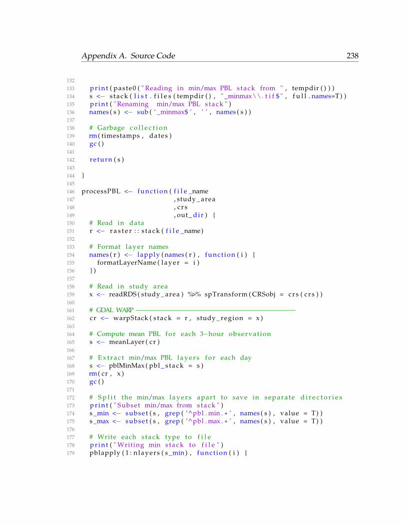
Appendix A. Source Code 238
132133 p r i n t ( paste0 ( " Reading in min/max PBL stack from " , tempdir ( ) ) )134 s <− s tack ( l i s t . f i l e s ( tempdir ( ) , " _minmax\\. t i f $ " , f u l l . names=T ) )135 p r i n t ( " Renaming min/max PBL stack " )136 names ( s ) <− sub ( ’ _minmax$ ’ , ’ ’ , names ( s ) )137138 # Garbage c o l l e c t i o n139 rm( timestamps , dates )140 gc ( )141142 re turn ( s )143144 }145146 processPBL <− func t ion ( f i l e _name147 , study _ area148 , c r s149 , out _ d i r ) {150 # Read in data151 r <− r a s t e r : : s tack ( f i l e _name)152153 # Format l a y e r names154 names ( r ) <− lapply ( names ( r ) , func t ion ( i ) {155 formatLayerName ( l a y e r = i )156 } )157158 # Read in study area159 x <− readRDS ( study _ area ) %>% spTransform ( CRSobj = c r s ( c r s ) )160161 # GDAL WARP −−−−−−−−−−−−−−−−−−−−−−−−−−−−−−−−−−−−−−−−162 cr <− warpStack ( s tack = r , study _ region = x )163164 # Compute mean PBL f o r each 3−hour observat ion165 s <− meanLayer ( cr )166167 # E x t r a c t min/max PBL l a y e r s f o r each day168 s <− pblMinMax ( pbl _ s tack = s )169 rm( cr , x )170 gc ( )171172 # S p l i t the min/max l a y e r s apart to save in separa te d i r e c t o r i e s173 p r i n t ( " Subset min/max from stack " )174 s _min <− subset ( s , grep ( ’^pbl . min . * ’ , names ( s ) , value = T ) )175 s _max <− subset ( s , grep ( ’^pbl . max . * ’ , names ( s ) , value = T ) )176177 # Write each s tack type to f i l e178 p r i n t ( " Writing min s tack to f i l e " )179 pblapply ( 1 : n layers ( s _min ) , func t ion ( i ) {
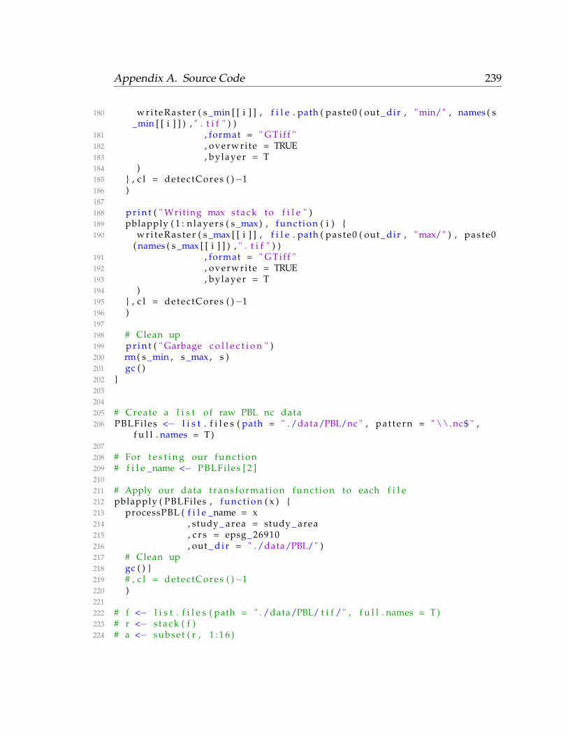
Appendix A. Source Code 239
180 wri teRas ter ( s _min [ [ i ] ] , f i l e . path ( paste0 ( out _ dir , " min/" , names ( s_min [ [ i ] ] ) , " . t i f " ) )
181 , format = " GTif f "182 , overwrite = TRUE183 , bylayer = T184 )185 } , c l = detectCores ( )−1186 )187188 p r i n t ( " Writing max s tack to f i l e " )189 pblapply ( 1 : n layers ( s _max) , func t ion ( i ) {190 wri teRas ter ( s _max [ [ i ] ] , f i l e . path ( paste0 ( out _ dir , "max/" ) , paste0
( names ( s _max [ [ i ] ] ) , " . t i f " ) )191 , format = " GTif f "192 , overwrite = TRUE193 , bylayer = T194 )195 } , c l = detectCores ( )−1196 )197198 # Clean up199 p r i n t ( " Garbage c o l l e c t i o n " )200 rm( s _min , s _max , s )201 gc ( )202 }203204205 # Create a l i s t of raw PBL nc data206 PBLFiles <− l i s t . f i l e s ( path = " . /data/PBL/nc " , pa t te rn = " \\. nc$ " ,
f u l l . names = T )207208 # For t e s t i n g our funct ion209 # f i l e _name <− PBLFiles [ 2 ]210211 # Apply our data transformat ion funct ion to each f i l e212 pblapply ( PBLFiles , func t ion ( x ) {213 processPBL ( f i l e _name = x214 , study _ area = study _ area215 , c r s = epsg_ 26910216 , out _ d i r = " . /data/PBL/" )217 # Clean up218 gc ( ) }219 # , c l = detectCores ( )−1220 )221222 # f <− l i s t . f i l e s ( path = " . /data/PBL/ t i f / " , f u l l . names = T )223 # r <− s tack ( f )224 # a <− subset ( r , 1 : 1 6 )
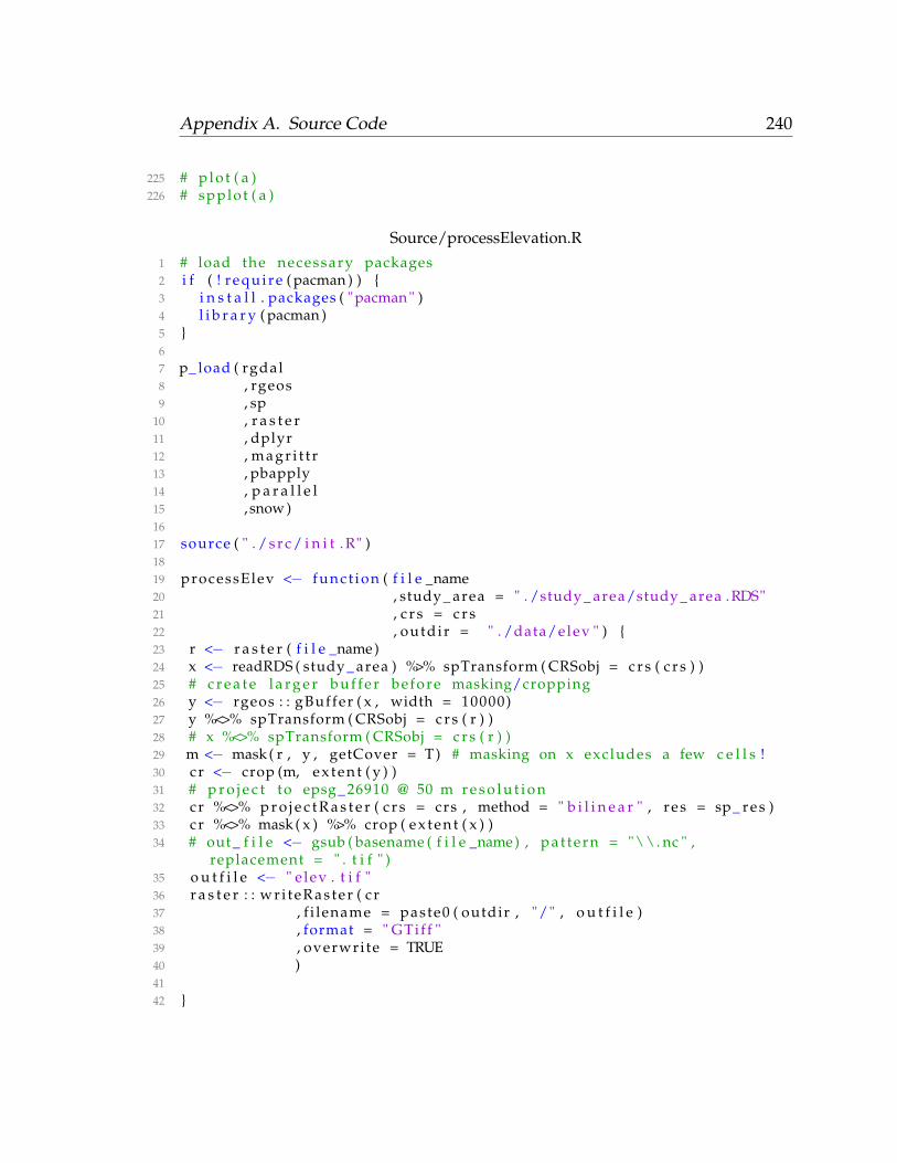
Appendix A. Source Code 240
225 # p l o t ( a )226 # spplot ( a )
Source/processElevation.R1 # load the necessary packages2 i f ( ! r equi re ( pacman ) ) {3 i n s t a l l . packages ( " pacman " )4 l i b r a r y ( pacman )5 }67 p_ load ( rgdal8 , rgeos9 , sp
10 , r a s t e r11 , dplyr12 , ma gr i t t r13 , pbapply14 , p a r a l l e l15 , snow )1617 source ( " . / s r c / i n i t . R" )1819 processElev <− func t ion ( f i l e _name20 , study _ area = " . /study _ area/study _ area . RDS"21 , c r s = c r s22 , outdir = " . /data/elev " ) {23 r <− r a s t e r ( f i l e _name)24 x <− readRDS ( study _ area ) %>% spTransform ( CRSobj = c r s ( c r s ) )25 # c r e a t e l a r g e r b u f f e r before masking/cropping26 y <− rgeos : : gBuffer ( x , width = 10000)27 y %<>% spTransform ( CRSobj = c r s ( r ) )28 # x %<>% spTransform ( CRSobj = c r s ( r ) )29 m <− mask ( r , y , getCover = T ) # masking on x excludes a few c e l l s !30 cr <− crop (m, e x t e n t ( y ) )31 # p r o j e c t to epsg_ 26910 @ 50 m r e s o l u t i o n32 cr %<>% p r o j e c t R a s t e r ( c r s = crs , method = " b i l i n e a r " , re s = sp_ re s )33 cr %<>% mask ( x ) %>% crop ( e x t e n t ( x ) )34 # out _ f i l e <− gsub ( basename ( f i l e _name) , pa t te rn = "\\. nc " ,
replacement = " . t i f " )35 o u t f i l e <− " e lev . t i f "36 r a s t e r : : wr i teRas ter ( cr37 , f i lename = paste0 ( outdir , "/" , o u t f i l e )38 , format = " GTif f "39 , overwrite = TRUE40 )4142 }
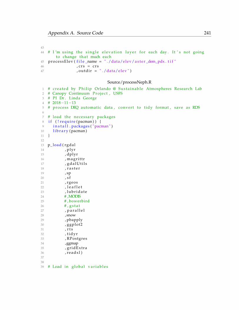
Appendix A. Source Code 241
4344 # I ’m using the s i n g l e e l e v a t i o n l a y e r f o r each day . I t ’ s not going
to change t h a t much each45 processElev ( f i l e _name = " . /data/elev/ a s t e r _dem_pdx . t i f "46 , c r s = c r s47 , outdir = " . /data/elev " )
Source/processNeph.R1 # crea ted by P h i l i p Orlando @ S u s t a i n a b l e Atmospheres Research Lab2 # Canopy Continuum P r o j e c t , USFS3 # PI Dr . Linda George4 # 2018−11−135 # process DEQ automatic data , convert to t idy format , save as RDS67 # load the necessary packages8 i f ( ! r equi re ( pacman ) ) {9 i n s t a l l . packages ( " pacman " )
10 l i b r a r y ( pacman )11 }1213 p_ load ( rgdal14 , p lyr15 , dplyr16 , ma gr i t t r17 , g d a l U t i l s18 , r a s t e r19 , sp20 , s f21 , rgeos22 , l e a f l e t23 , l u b r i d a t e24 # ,MODIS25 # , bowerbird26 # , g s t a t27 , p a r a l l e l28 , snow29 , pbapply30 , ggplot231 , r t s32 , t i d y r33 , RPostgres34 ,ggmap35 , gr idExtra36 , readxl )373839 # Load in g loba l v a r i a b l e s
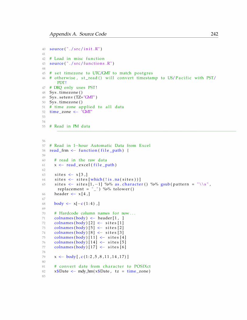
Appendix A. Source Code 242
40 source ( " . / s r c / i n i t . R" )4142 # Load in misc funct ion43 source ( " . / s r c /f u n c t i o n s . R" )4445 # s e t timezone to UTC/GMT to match postgres46 # otherwise , s t _ read ( ) w i l l convert timestamp to US/ P a c i f i c with PST/
PDT!47 # DEQ only uses PST !48 Sys . timezone ( )49 Sys . setenv (TZ="GMT" )50 Sys . timezone ( )51 # time zone applied to a l l data52 time _zone <− "GMT"535455 # Read in PM data
−−−−−−−−−−−−−−−−−−−−−−−−−−−−−−−−−−−−−−−−−−−−−−−−−−−−−−−−−−−−−−−−−−−−−−−−−−
5657 # Read in 1−hour Automatic Data from Excel58 read _frm <− func t ion ( f i l e _ path ) {5960 # read in the raw data61 x <− read _ e x c e l ( f i l e _ path )6263 s i t e s <− x [ 3 , ]64 s i t e s <− s i t e s [ which ( ! i s . na ( s i t e s ) ) ]65 s i t e s <− s i t e s [1 , −1] %>% as . c h a r a c t e r ( ) %>% gsub ( pat te rn = "\\s " ,
replacement = " _ " ) %>% tolower ( )66 header <− x [ 4 , ]6768 body <− x[−c ( 1 : 4 ) , ]6970 # Hardcode column names f o r now . . .71 colnames ( body ) <− header [ 1 , ]72 colnames ( body ) [ 2 ] <− s i t e s [ 1 ]73 colnames ( body ) [ 5 ] <− s i t e s [ 2 ]74 colnames ( body ) [ 8 ] <− s i t e s [ 3 ]75 colnames ( body ) [ 1 1 ] <− s i t e s [ 4 ]76 colnames ( body ) [ 1 4 ] <− s i t e s [ 5 ]77 colnames ( body ) [ 1 7 ] <− s i t e s [ 6 ]7879 x <− body [ , c ( 1 : 2 , 5 , 8 , 1 1 , 1 4 , 1 7 ) ]8081 # convert date from c h a r a c t e r to POSIXct82 x$Date <− mdy_hm( x$Date , tz = time _zone )83
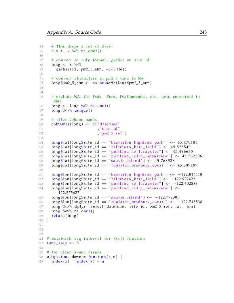
Appendix A. Source Code 243
84 # This drops a l o t of days !85 # x <− x %>% na . omit ( )8687 # convert to t idy format , gather on s i t e id88 long <− x %>%89 gather ( id , pm2_5_atm , −c ( Date ) )9091 # convert c h a r a c t e r s in pm2_5 data to NA92 long $pm2_5_atm <− as . numeric ( long $pm2_5_atm )939495 # exclude NAs (No Data , Zero , DL/Computer , e t c . ge t s converted to
NA)96 long <− long %>% na . omit ( )97 long %<>% unique ( )9899 # a l t e r column names
100 colnames ( long ) <− c ( " datetime "101 , " s i t e _ id "102 , "pm2_5_ r e f " )103104 long $ l a t [ long $ s i t e _ id == " beaverton _ highland _park " ] <− 45 .470183105 long $ l a t [ long $ s i t e _ id == " h i l l s b o r o _ hare _ f i e l d " ] <− 45 .528549106 long $ l a t [ long $ s i t e _ id == " port land _ se _ l a f a y e t t e " ] <− 45 .496635107 long $ l a t [ long $ s i t e _ id == " port land _ c u l l y _ helensview " ] <− 45 .562206108 long $ l a t [ long $ s i t e _ id == " sauvie _ i s l a n d " ] <− 45 .768528109 long $ l a t [ long $ s i t e _ id == " t u a l a t i n _bradbury_ court " ] <− 45 .399189110111 long $ lon [ long $ s i t e _ id == " beaverton _ highland _park " ] <− −122.816418112 long $ lon [ long $ s i t e _ id == " h i l l s b o r o _ hare _ f i e l d " ] <− −122.972423113 long $ lon [ long $ s i t e _ id == " port land _ se _ l a f a y e t t e " ] <− −122.602883114 long $ lon [ long $ s i t e _ id == " port land _ c u l l y _ helensview " ] <−
−122.575627115 long $ lon [ long $ s i t e _ id == " sauvie _ i s l a n d " ] <− −122.772305116 long $ lon [ long $ s i t e _ id == " t u a l a t i n _bradbury_ court " ] <− −122.745538117 long %<>% dplyr : : s e l e c t ( datetime , s i t e _ id , pm2_5_ ref , l a t , lon )118 long %<>% na . omit ( )119 re turn ( long )120 }121122123124 # e s t a b l i s h avg i n t e r v a l f o r x t s ( ) func t ion125 time _ step <− 5126127 # f o r c lean 5−min breaks128 a l i g n . time . down = funct ion ( x , n ) {129 index ( x ) = index ( x ) − n
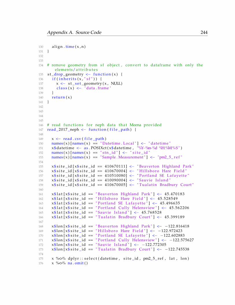
Appendix A. Source Code 244
130 a l i g n . time ( x , n )131 }132133134 # remove geometry from s f o b j e c t , convert to dataframe with only the
elements/ a t t r i b u t e s135 s t _drop_geometry <− func t ion ( x ) {136 i f ( i n h e r i t s ( x , " s f " ) ) {137 x <− s t _ s e t _geometry ( x , NULL)138 c l a s s ( x ) <− ’ data . frame ’139 }140 re turn ( x )141 }142143144145146 # read f u n c t i o n s f o r neph data t h a t Meena provided147 read _ 2017 _neph <− func t ion ( f i l e _ path ) {148149 x <− read . csv ( f i l e _ path )150 names ( x ) [ names ( x ) == " Datetime . Local " ] <− " datetime "151 x$ datetime <− as . POSIXct ( x$ datetime , "%Y−%m−%d %H:%M:%S " )152 names ( x ) [ names ( x ) == " s tn _ id " ] <− " s i t e _ id "153 names ( x ) [ names ( x ) == " Sample . Measurement " ] <− "pm2_5_ r e f "154155 x$ s i t e _ id [ x$ s i t e _ id == 410670111] <− " Beaverton Highland Park "156 x$ s i t e _ id [ x$ s i t e _ id == 410670004] <− " Hi l l sboro Hare F i e l d "157 x$ s i t e _ id [ x$ s i t e _ id == 410510080] <− " Port land SE L a f a y e t t e "158 x$ s i t e _ id [ x$ s i t e _ id == 410090004] <− " Sauvie Is land "159 x$ s i t e _ id [ x$ s i t e _ id == 410670005] <− " Tuala t in Bradbury Court "160161 x$ l a t [ x$ s i t e _ id == " Beaverton Highland Park " ] <− 45 .470183162 x$ l a t [ x$ s i t e _ id == " Hi l l sboro Hare F i e l d " ] <− 45 .528549163 x$ l a t [ x$ s i t e _ id == " Port land SE L a f a y e t t e " ] <− 45 .496635164 x$ l a t [ x$ s i t e _ id == " Port land Cully Helensview " ] <− 45 .562206165 x$ l a t [ x$ s i t e _ id == " Sauvie Is land " ] <− 45 .768528166 x$ l a t [ x$ s i t e _ id == " Tuala t in Bradbury Court " ] <− 45 .399189167168 x$ lon [ x$ s i t e _ id == " Beaverton Highland Park " ] <− −122.816418169 x$ lon [ x$ s i t e _ id == " Hi l l sboro Hare F i e l d " ] <− −122.972423170 x$ lon [ x$ s i t e _ id == " Port land SE L a f a y e t t e " ] <− −122.602883171 x$ lon [ x$ s i t e _ id == " Port land Cully Helensview " ] <− −122.575627172 x$ lon [ x$ s i t e _ id == " Sauvie Is land " ] <− −122.772305173 x$ lon [ x$ s i t e _ id == " Tuala t in Bradbury Court " ] <− −122.745538174175 x %<>% dplyr : : s e l e c t ( datetime , s i t e _ id , pm2_5_ ref , l a t , lon )176 x %<>% na . omit ( )
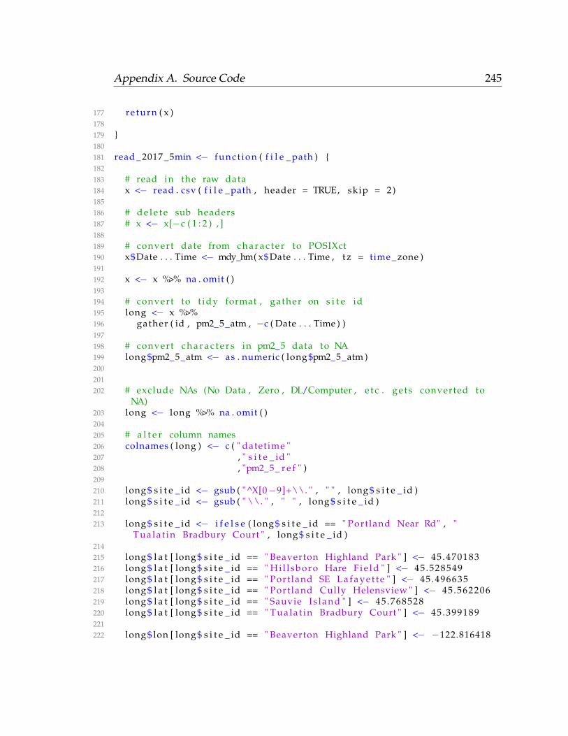
Appendix A. Source Code 245
177 re turn ( x )178179 }180181 read _ 2017 _5min <− func t ion ( f i l e _ path ) {182183 # read in the raw data184 x <− read . csv ( f i l e _path , header = TRUE, skip = 2)185186 # d e l e t e sub headers187 # x <− x[−c ( 1 : 2 ) , ]188189 # convert date from c h a r a c t e r to POSIXct190 x$Date . . . Time <− mdy_hm( x$Date . . . Time , tz = time _zone )191192 x <− x %>% na . omit ( )193194 # convert to t idy format , gather on s i t e id195 long <− x %>%196 gather ( id , pm2_5_atm , −c ( Date . . . Time ) )197198 # convert c h a r a c t e r s in pm2_5 data to NA199 long $pm2_5_atm <− as . numeric ( long $pm2_5_atm )200201202 # exclude NAs (No Data , Zero , DL/Computer , e t c . ge t s converted to
NA)203 long <− long %>% na . omit ( )204205 # a l t e r column names206 colnames ( long ) <− c ( " datetime "207 , " s i t e _ id "208 , "pm2_5_ r e f " )209210 long $ s i t e _ id <− gsub ( "^X[0−9]+\\. " , " " , long $ s i t e _ id )211 long $ s i t e _ id <− gsub ( " \\. " , " " , long $ s i t e _ id )212213 long $ s i t e _ id <− i f e l s e ( long $ s i t e _ id == " Port land Near Rd" , "
Tuala t in Bradbury Court " , long $ s i t e _ id )214215 long $ l a t [ long $ s i t e _ id == " Beaverton Highland Park " ] <− 45 .470183216 long $ l a t [ long $ s i t e _ id == " Hi l l sboro Hare F i e l d " ] <− 45 .528549217 long $ l a t [ long $ s i t e _ id == " Port land SE L a f a y e t t e " ] <− 45 .496635218 long $ l a t [ long $ s i t e _ id == " Port land Cully Helensview " ] <− 45 .562206219 long $ l a t [ long $ s i t e _ id == " Sauvie I s land " ] <− 45 .768528220 long $ l a t [ long $ s i t e _ id == " Tuala t in Bradbury Court " ] <− 45 .399189221222 long $ lon [ long $ s i t e _ id == " Beaverton Highland Park " ] <− −122.816418
Appendix A. Source Code 246
223 long $ lon [ long $ s i t e _ id == " Hi l l sboro Hare F i e l d " ] <− −122.972423224 long $ lon [ long $ s i t e _ id == " Port land SE L a f a y e t t e " ] <− −122.602883225 long $ lon [ long $ s i t e _ id == " Port land Cully Helensview " ] <−
−122.575627226 long $ lon [ long $ s i t e _ id == " Sauvie I s land " ] <− −122.772305227 long $ lon [ long $ s i t e _ id == " Tuala t in Bradbury Court " ] <− −122.745538228229230 long %<>% dplyr : : s e l e c t ( datetime , s i t e _ id , pm2_5_ ref , l a t , lon )231 long %<>% na . omit ( )232233 long $ s i t e _ id <− gsub ( "\\ " , " _ " , long $ s i t e _ id )234 long $ s i t e _ id <− tolower ( long $ s i t e _ id )235 # long $ s i t e _ id <− s t r i n g r : : s t r _ r e p l a c e ( long $ s i t e _ id , " . " , " " )236237 re turn ( long )238239 }240241242 read _ 2018 _5min <− func t ion ( f i l e _ path ) {243244 # read in the raw data245 x <− read _ e x c e l ( f i l e _ path )246247 # d e l e t e sub headers248 x <− x[−c ( 1 : 2 ) , ]249 x <− x [ , 2 : ncol ( x ) ]250 names ( x ) [ names ( x ) == " Date & Time − s t a r t of obs period " ] <− " Date "251 # convert date from c h a r a c t e r to POSIXct252 x$Date <− ymd_hms( x$Date , tz = time _zone )253 x <− x %>% na . omit ( )254255 # convert to t idy format , gather on s i t e id256 long <− x %>%257 gather ( id , pm2_5_atm , −c ( Date ) )258259 # convert c h a r a c t e r s in pm2_5 data to NA260 long $pm2_5_atm <− as . numeric ( long $pm2_5_atm )261262263 # exclude NAs (No Data , Zero , DL/Computer , e t c . ge t s converted to
NA)264 long <− long %>% na . omit ( )265266 # a l t e r column names267 colnames ( long ) <− c ( " datetime "268 , " s i t e _ id "
Appendix A. Source Code 247
269 , "pm2_5_ r e f " )270271 # long $ s i t e _ id <− gsub ( "^X[0 −9]+\\." , " " , long $ s i t e _ id )272 # long $ s i t e _ id <− gsub ( " \ \ . " , " " , long $ s i t e _ id )273274 long $ s i t e _ id <− i f e l s e ( long $ s i t e _ id == " Port land Near Rd" , "
Tuala t in Bradbury Court " , long $ s i t e _ id )275276 long $ l a t [ long $ s i t e _ id == " Beaverton Highland Park " ] <− 45 .470183277 long $ l a t [ long $ s i t e _ id == " Hi l l sboro Hare F i e l d " ] <− 45 .528549278 long $ l a t [ long $ s i t e _ id == " Port land SE L a f a y e t t e " ] <− 45 .496635279 long $ l a t [ long $ s i t e _ id == " Port land Cully Helensview " ] <− 45 .562206280 long $ l a t [ long $ s i t e _ id == " Sauvie I s land " ] <− 45 .768528281 long $ l a t [ long $ s i t e _ id == " Tuala t in Bradbury Court " ] <− 45 .399189282283 long $ lon [ long $ s i t e _ id == " Beaverton Highland Park " ] <− −122.816418284 long $ lon [ long $ s i t e _ id == " Hi l l sboro Hare F i e l d " ] <− −122.972423285 long $ lon [ long $ s i t e _ id == " Port land SE L a f a y e t t e " ] <− −122.602883286 long $ lon [ long $ s i t e _ id == " Port land Cully Helensview " ] <−
−122.575627287 long $ lon [ long $ s i t e _ id == " Sauvie I s land " ] <− −122.772305288 long $ lon [ long $ s i t e _ id == " Tuala t in Bradbury Court " ] <− −122.745538289290291 long %<>% dplyr : : s e l e c t ( datetime , s i t e _ id , pm2_5_ ref , l a t , lon )292 long %<>% na . omit ( )293294 long $ s i t e _ id <− gsub ( "\\ " , " _ " , long $ s i t e _ id )295 long $ s i t e _ id <− tolower ( long $ s i t e _ id )296 # long $ s i t e _ id <− s t r i n g r : : s t r _ r e p l a c e ( long $ s i t e _ id , " . " , " " )297298 re turn ( long )299300 }301302 read _ 2018 _neph <− func t ion ( f i l e _ path ) {303304 # e x t r a c t header305 header <− read . csv ( f i l e _path , nrow = 1 , skip = 2 , header = FALSE ,
s t r i n g s A s F a c t o r s = FALSE) %>%306 s e l e c t _ i f ( ~ ! any ( i s . na ( . ) ) )307308 # e x t r a c t body309 x <− read . csv ( f i l e _path , header = TRUE, skip = 4 , s t r i n g s A s F a c t o r s
= FALSE)310311 colnames ( header ) <− u n l i s t ( header [ 1 , ] )312 colnames ( x ) <− colnames ( header )

Appendix A. Source Code 248
313314 names ( x ) [ names ( x ) == " Date & Time " ] <− " datetime "315 x$ datetime <− as . POSIXct ( x$ datetime , format = ’%m/%d/%Y %H:%M’ )316 x <− x %>%317 gather ( key = s i t e _ id , value = pm2_5_ ref , −datetime )318 x$pm2_5_ r e f <− as . numeric ( x$pm2_5_ r e f )319 x <− x %>% na . omit ( )320 x$ l a t [ x$ s i t e _ id == " Beaverton Highland Park " ] <− 45 .470183321 x$ l a t [ x$ s i t e _ id == " Hi l l sboro Hare F i e l d " ] <− 45 .528549322 x$ l a t [ x$ s i t e _ id == " Port land SE L a f a y e t t e " ] <− 45 .496635323 x$ l a t [ x$ s i t e _ id == " Port land Cully Helensview " ] <− 45 .562206324 x$ l a t [ x$ s i t e _ id == " Sauvie I s land " ] <− 45 .768528325 x$ l a t [ x$ s i t e _ id == " Tuala t in Bradbury Court " ] <− 45 .399189326327 x$ lon [ x$ s i t e _ id == " Beaverton Highland Park " ] <− −122.816418328 x$ lon [ x$ s i t e _ id == " Hi l l sboro Hare F i e l d " ] <− −122.972423329 x$ lon [ x$ s i t e _ id == " Port land SE L a f a y e t t e " ] <− −122.602883330 x$ lon [ x$ s i t e _ id == " Port land Cully Helensview " ] <− −122.575627331 x$ lon [ x$ s i t e _ id == " Sauvie I s land " ] <− −122.772305332 x$ lon [ x$ s i t e _ id == " Tuala t in Bradbury Court " ] <− −122.745538333334 re turn ( x )335336 }337338 neph2017 <− read _ 2017 _5min ( " . /data/frm/bhp_ hhf _ tbc _ s e l _5min_pm25_
20170701 _ to _ 20180918 . csv " )339 neph2018 <− read _ 2018 _5min ( " . /data/frm/pm25_5min_bhp_ hhf_pch_ s e l _ s i s _
tbc _ sep18 _ to _may19 . x l s x " )340341 # TODO Sauvie Is land i s missing from 2017 data !342343 # convert ing from hourly to dai ly , computing min , max , mean , sd344 neph <− rbind ( neph2017 , neph2018 )345346 # remove any d u p l i c a t e s ( e . g . September 2018)347 neph %<>% unique ( )348349 neph$ date <− l u b r i d a t e : : date ( neph$ datetime )350351 neph_ da i ly <− neph %>% dplyr : : s e l e c t (−datetime ) %>% group_by ( date ,
s i t e _ id , l a t , lon ) %>%352 summarize_ i f ( i s . numeric353 , funs (pm2 . 5 . mean = mean354 ,pm2 . 5 . min = min355 ,pm2 . 5 . max = max356 ,pm2 . 5 . sd = sd357 ,pm2 . 5 . median = median )

Appendix A. Source Code 249
358 , na . rm = T )359360 neph %<>% s t _ as _ s f ( coords = c ( " lon " , " l a t " ) , c r s = wgs_ 84)361 neph_ da i ly %<>% s t _ as _ s f ( coords = c ( " lon " , " l a t " ) , c r s = wgs_ 84)362 # I n s pe c t the data and clean up o u t l i e r s363 summary ( neph )364 summary ( neph_ da i l y )365366 # Yikes there are d e f i n i t e l y some i s s u e s with the mean/max values367 p l o t ( neph_ da i ly $ date , neph_ da i ly $pm2 . 5 . mean)368369 # Let ’ s f i l t e r by our max pm range i n i t v a r i a b l e ( 2 5 0 )370 neph_ da i ly %<>% f i l t e r (pm2 . 5 . mean <= max_pm_ range )371 summary ( neph_ da i l y )372373 neph %<>% f i l t e r (pm2_5_ r e f <= max_pm_ range )374 summary ( neph )375376 # Looks a l o t b e t t e r now377 p l o t ( neph_ da i ly $ date , neph_ da i ly $pm2 . 5 . mean)378379 # TODO Create neph 15−minute averages ?380381 # Write our c lean neph data to f i l e382 saveRDS ( neph_ dai ly , " . /data/deq/neph1day . RDS" )383 saveRDS ( neph , " . /data/deq/neph5min . RDS" )384385 neph <− read _frm ( " . /data/frm/AutomaticData5_29_ 2019 . x l s x " )386 neph %<>% s t _ as _ s f ( coords = c ( " lon " , " l a t " ) , c r s = wgs_ 84)387 neph %<>% f i l t e r (pm2_5_ r e f <= max_pm_ range )388 saveRDS ( neph , " . /data/deq/neph1hour . RDS" )
Source/processPurpleAir.R1 # crea ted by P h i l i p Orlando @ S u s t a i n a b l e Atmospheres Research Lab2 # Canopy Continuum P r o j e c t , USFS3 # PI Dr . Linda George4 # 2018−11−285 # pul l PurpleAir data from database and c r e a t e da i ly averages67 # load the necessary packages8 i f ( ! r equi re ( pacman ) ) {9 i n s t a l l . packages ( " pacman " )
10 l i b r a r y ( pacman )11 }1213 p_ load ( rgdal14 , p lyr
Appendix A. Source Code 250
15 , dplyr16 , ma gr i t t r17 , g d a l U t i l s18 , r a s t e r19 , sp20 , s f21 , rgeos22 , p a r a l l e l23 , l u b r i d a t e24 , ggplot225 , r t s26 , RPostgres27 ,ggmap28 , g r idExtra )2930 source ( " . / s r c /f u n c t i o n s . R" )31 source ( " . / s r c / i n i t . R" )3233 # s e t timezone
−−−−−−−−−−−−−−−−−−−−−−−−−−−−−−−−−−−−−−−−−−−−−−−−−−−−−−−−−−−−−−−−−−−−−−−−−−−−−
3435 # s e t timezone to UTC/GMT to match postgres36 # otherwise , s t _ read ( ) w i l l convert timestamp to US/ P a c i f i c with PST/
PDT!37 # DEQ only uses PST !38 Sys . timezone ( )39 Sys . setenv (TZ="GMT" )40 Sys . timezone ( )4142 # Connect to Database
−−−−−−−−−−−−−−−−−−−−−−−−−−−−−−−−−−−−−−−−−−−−−−−−−−−−−−−−−−−−−−−−−−−−−−
4344 ## connect ing to l o c a l db45 host <− ’ pgsql120 . rc . pdx . edu ’46 db <− ’ canopycontinuum ’47 user <− ’ porlando ’48 port <− 543349 pw <− scan ( " . / b a t t e r i e s . pgpss " , what = " " ) # in parent d i r505152 # open connect ion to our db53 con <− dbConnect ( drv = RPostgres : : Postgres ( )54 ,dbname = db55 , host = ’ pgsql102 . rc . pdx . edu ’ # not sure why o b j e c t
host isn ’ t working . . .56 , port = port
Appendix A. Source Code 251
57 , password = pw58 , user = user )5960 # Reading in hourly PurpleAir data
−−−−−−−−−−−−−−−−−−−−−−−−−−−−−−−−−−−−−−−−−−−−−−−−−−−−−−−−−−−−−−−−−−−−−−−−
6162 # Add s e l e c t d i s t i n c t subquery i n t o t h i s l a t e r !63 # pa_h <− s t _ read ( dsn = con64 # # ,geom_column = "geom"65 # # ,EWKB = TRUE66 # , query = paste0 ( " SELECT date _ trunc ( ’ hour ’ , c rea ted _
a t ) hourly , l a b e l , avg (pm2_5_atm ) , geom67 # FROM pdx68 # GROUP BY l a b e l , date _ trunc ( ’ hour ’ , c rea ted _
a t ) , geom ; " ) )6970 # pa_h <− s t _ read ( dsn = con71 # # ,geom_column = "geom" # depreceated !72 # # ,EWKB = TRUE73 # , query = paste0 ( " SELECT date ( a . c rea ted _ a t ) , date _ part
( ’ hour ’ , a . c rea ted _ at ) as hour , a . id , a . sensor , a . l a b e l , avg ( a . pm2_5_atm ) pm2_5_atm , a . geom
74 # FROM (SELECT DISTINCT * FROM pdxWHERE created _ a t >= ’ "
75 # , l u b r i d a t e : : ymd( s t a r t _ date ) + hours( 8 )
76 # , " ’ AND created _ a t <= ’ "77 # , l u b r i d a t e : : ymd( end_ date ) + hours ( 8 ) ,
" ’ ) a78 # GROUP BY a . id , a . sensor , a . l a b e l , a .
geom , date ( a . c rea ted _ at ) , date _ part ( ’ hour ’ , a . c rea ted _ at ) ; " )79 # )808182 # Reading in PurpleAir data
−−−−−−−−−−−−−−−−−−−−−−−−−−−−−−−−−−−−−−−−−−−−−−−−−−−−−−−−−−−−−−−−−−−−−−−−
83 # s t a r t _ date <− "2017−07−01"84 #end_ date <− "2018−10−20"8586 pa <− s t _ read ( dsn = con87 # ,geom_column = "geom" # depreceated !88 # ,EWKB = TRUE89 , query = paste0 ( "SELECT DISTINCT * FROM pdx WHERE
created _ a t >= ’ "90 , l u b r i d a t e : : ymd( s t a r t _ date ) + hours ( 8 )91 , " ’ AND created _ a t <= ’ "
Appendix A. Source Code 252
92 , l u b r i d a t e : : ymd( end_ date ) + hours ( 8 ) , "’ ; " )
93 )9495 # convert from UTC to UTC−8 or PST ( same as DEQ)96 pa$ crea ted _ at <− l u b r i d a t e : : ymd_hms( pa$ crea ted _ a t ) − l u b r i d a t e : : hours
( 8 )9798 # rename the datetime column99 names ( pa ) [ names ( pa ) == " crea ted _ a t " ] <− " datetime "
100101 # check the time zone of pa data102 a t t r ( pa$ datetime , " tzone " )103104 # s e t SRID105 s t _ c r s ( pa ) <− epsg_ 26910106 pa$ date <− l u b r i d a t e : : date ( pa$ datetime )107 head ( pa )108109 # Apply Indiv idual Correc t ion F a c t o r s each sensor (Aug 2018)
−−−−−−−−−−−−−−−−−−−−−−−−−−−−−−−−−−−−−−−110 pa_ c f <− s t _ read ( dsn = con111 # ,geom_column = "geom"112 # ,EWKB = TRUE113 , query = "SELECT DISTINCT * FROM pdx_ c f ; " )114115116 # remove geom f o r now . . .117 pa %<>% s t _drop_geometry ( )118 pa_ c f %<>% s t _drop_geometry ( )119 # pa_ c f $ year %<>% as . i n t e g e r ( )120 pa$ id %<>% as . i n t e g e r ( )121122 # # Find the CF with the maximum R2 f o r each sensor , excluding
anything below 0 . 8123 # pa_ c f %<>%124 # group_by ( id , l a b e l ) %>%125 # # use the month with highes t c o r r e l a t i o n ( inc ludes August 2017
f o r some sensors )126 # # f i l t e r ( year == 2018 & month == "Aug " ) %>%127 # s l i c e ( which . max( r _ squared ) ) %>%128 # f i l t e r ( r _ squared > 0 . 8 5 ) %>%129 # na . omit ( )130131 # j o i n CF and PA data132 pa %<>% inner _ j o i n ( pa_ c f %>% dplyr : : s e l e c t ( c ( id , l a b e l , r _squared ,
slope , i n t e r c e p t ) ) ) %>%133 dplyr : : s e l e c t ( c ( datetime , id , l a b e l , everything ( ) ) )
Appendix A. Source Code 253
134135 # apply c o r r e c t i o n f a c t o r136 pa$pm2_5_ c f _x <− ( pa$pm2_5_atm * pa$ slope ) +pa$ i n t e r c e p t137138 # i n s p e c t the new data ( compare with lm f i g u r e s )139 pa %>% dplyr : : s e l e c t ( c ( datetime , l a b e l , id , slope , pm2_5_atm , pm2_5_
c f _x , r _ squared ) ) %>%140 f i l t e r ( datetime == as . Date ( " 2018−08−01 " ) ) %>%141 arrange ( l a b e l )142143 # i n s p e c t raw data and cleaned data144 pa %>% dplyr : : f i l t e r ( r _ squared > 0 . 8 5 ) %>% ggplot ( aes ( x = l a b e l , y =
pm2_5_ c f _x ) ) +145 geom_ boxplot ( ) +146 theme ( a x i s . t e x t . x = element _ t e x t ( angle = 45 , h j u s t = 1) )147148 pa %>% f i l t e r (pm2_5_ c f _x < max_pm_ range & r _ squared > 0 . 8 5 & slope >=
0 . 4 & slope <= 1 . 6 ) %>%149 na . omit ( ) %>%150 dplyr : : f i l t e r ( r _ squared > 0 . 8 ) %>% ggplot ( aes ( x = l a b e l , y = pm2_5_
c f _x ) ) +151 geom_ boxplot ( ) +152 theme ( a x i s . t e x t . x = element _ t e x t ( angle = 45 , h j u s t = 1) )153154 pa %>% f i l t e r (pm2_5_ c f _x < max_pm_ range & r _ squared > 0 . 8 5 & slope >=
0 . 4 & slope <= 1 . 6 ) %>%155 na . omit ( ) %>%156 dplyr : : f i l t e r ( r _ squared > 0 . 8 ) %>% ggplot ( aes ( x = as . f a c t o r ( id ) , y
= slope ) ) +157 geom_ boxplot ( ) +158 theme ( a x i s . t e x t . x = element _ t e x t ( angle = 45 , h j u s t = 1) )159160 pa_ c f %>% ggplot ( aes ( x = 1 , y = slope , f i l l = as . f a c t o r ( 1 ) ) ) + geom_
v i o l i n ( ) + xlab ( " " ) +161 theme_minimal ( ) + g g t i t l e ( " PurpleAir C a l i b r a t i o n F a c t o r s " ) +162 theme ( legend . t i t l e = element _ blank ( ) , legend . p o s i t i o n = " none " ,
a x i s . t e x t . x = element _ blank ( ) )163164 pa_ c f %>% ggplot ( aes ( x = 1 , y = r _squared , f i l l = as . f a c t o r ( 1 ) ) ) +
geom_ v i o l i n ( ) + xlab ( " " ) +165 theme_minimal ( ) + g g t i t l e ( " PurpleAir C a l i b r a t i o n F a c t o r s " ) +166 theme ( legend . t i t l e = element _ blank ( ) , legend . p o s i t i o n = " none " ,
a x i s . t e x t . x = element _ blank ( ) )167168169 # Remove f a u l t y sensors
−−−−−−−−−−−−−−−−−−−−−−−−−−−−−−−−−−−−−−−−−−−−−−−−−−−−−−−−−−−−−−−−−−−−−−−−−−−−−−
Appendix A. Source Code 254
170 pa_ f l a g <− s t _ read ( dsn = con171 # ,geom_column = "geom"172 # ,EWKB = T173 , query = "SELECT DISTINCT * FROM pdx_ f l a g ; " )174175176 # examine q u a l i t y of f l a g g i n g on suspect sensors177 top _ f l a g <− pa_ f l a g %>% f i l t e r ( f l a g == 1) %>%178 dplyr : : s e l e c t ( l a b e l , id ) %>%179 group_by ( l a b e l , id ) %>%180 mutate ( n = n ( ) ) %>%181 summarise_ i f ( i s . numeric , mean) %>%182 arrange ( desc ( n ) )183184 # ensure id column type matches pa185 pa$ id <− as . c h a r a c t e r ( pa$ id )186187 # With pdx_ f l a g == 0
−−−−−−−−−−−−−−−−−−−−−−−−−−−−−−−−−−−−−−−−−−−−−−−−−−−−−−−−188 # TODO confirm o u t l i e r d e t e c t i o n algo i s not worthwhile with new CF
methods . . .189 # c leaning data by slope between 0 . 5 and 1 . 5 helps reduce a d d i t i o n a l
o u t l i e r s190 # pa_ c lean <− pa %>% inner _ j o i n ( pa_ f lag , by = c ( " date " , " id " , " l a b e l
" ) ) %>%191 # # exclude f a u l t y sensor data , and trim extremes192 # f i l t e r ( f l a g == 0 & pm2_5_ c f _x <= max_pm_ range & r _ squared >= 0 . 9 )193194 # Not using the pdx_ f l a g algo
−−−−−−−−−−−−−−−−−−−−−−−−−−−−−−−−−−−−−−−−−−−−−−195 pa_ c lean <− pa %>% inner _ j o i n ( pa_ f lag , by = c ( " date " , " id " , " l a b e l " )
) %>%196 f i l t e r (pm2_5_ c f _x <= max_pm_ range & r _ squared >= 0 . 9 )197198 # pa_ d i r t y <− pa %>% l e f t _ j o i n ( pa_ f lag , by = c ( " date " , " id " , " l a b e l
" ) )199200 # pa_ f i l t e r <− pa %>% l e f t _ j o i n ( pa_ f lag , by = c ( " date " , " id " , " l a b e l
" ) ) %>%201 # # exclude f a u l t y sensor data , and trim extremes202 # f i l t e r (pm2_5_ c f _x <= max_pm_ range & r _ squared >= 0 . 8 5 & slope >=
0 . 5 & slope <= 1 . 5 )203204 nrow ( pa_ c lean ) /nrow ( pa )205206 pa_ c lean %>% ggplot ( aes ( x = l a b e l , y = pm2_5_ c f _x ) ) +207 geom_ v i o l i n ( ) +208 theme ( a x i s . t e x t . x = element _ t e x t ( angle = 45 , h j u s t = 1) )
Appendix A. Source Code 255
209210 # pa_ c lean <− pa %>%211 # f i l t e r (pm2_5_ c f _x < max_pm_ range & r _ squared > 0 . 8 5 & slope >=
0 . 4 & slope <= 1 . 6 ) %>%212 # na . omit ( )213214 pa_5m <− pa_ c lean %>%215 dplyr : : s e l e c t (−c ( date , geom) )216217 pa_summary <− pa_ c lean %>%218 dplyr : : s e l e c t (−datetime ) %>%219 group_by ( date , id , sensor , l a b e l ) %>%220 summarise_ a t ( "pm2_5_ c f _x " , funs ( mean , median , min , max) )221222 pa_summary$ d i f f <− abs ( pa_summary$mean − pa_summary$median )223224 pa_summary %>%225 group_by ( id , sensor , l a b e l ) %>%226 summarise_ a t ( " d i f f " , funs ( mean , median , max , min ) ) %>%227 arrange ( desc (max) )228229 pa_24h <− pa_ c lean %>%230 dplyr : : s e l e c t (−c ( datetime , geom) ) %>%231 group_by ( date , id , sensor , l a b e l ) %>%232 summarise_ i f ( i s . numeric , funs (mean) , na . rm = T )233234 pa_24h_ a l l <− pa_ d i r t y %>%235 dplyr : : s e l e c t (−c ( datetime , geom) ) %>%236 group_by ( date , id , sensor , l a b e l ) %>%237 summarise_ i f ( i s . numeric , funs (mean) , na . rm = T )238239 pa_24h_ f i l t e r <− pa_ f i l t e r %>%240 dplyr : : s e l e c t (−c ( datetime , geom) ) %>%241 group_by ( date , id , sensor , l a b e l ) %>%242 summarise_ i f ( i s . numeric , funs (mean) , na . rm = T )243244 pa_24h %>% ggplot ( aes ( x = l a b e l , y = pm2_5_ c f _x ) ) +245 geom_ boxplot ( ) +246 theme ( a x i s . t e x t . x = element _ t e x t ( angle = 45 , h j u s t = 1) )247248 pa_24h %>% ggplot ( aes ( x = date , y = pm2_5_ c f _x , c o l = f l a g ) ) +249 geom_ point ( ) +250 theme_bw( )251252 pa_24h_ a l l %>% f i l t e r (pm2_5_ c f _x <= max_pm_ range & l a b e l %in% top _
f l a g $ l a b e l ) %>% na . omit ( ) %>%253 ggplot ( aes ( x = date , y = pm2_5_ c f _x , c o l = as . f a c t o r ( f l a g ) ) ) +254 geom_ point ( alpha = 0 . 6 ) +
Appendix A. Source Code 256
255 theme_bw( ) +256 s c a l e _ c o l o r _manual ( values = c ( " #000000 " , " # ba2525 " ) ) +257 l a b s ( y = "PM2. 5 ( ug/m3) " , x = " " , c o l o r = " O u t l i e r Flag " , t i t l e = "
Modified Z−Score O u t l i e r Detect ion " ) +258 theme ( legend . p o s i t i o n =" bottom " )259260 pa_24h_ a l l %>% f i l t e r ( date >= " 2018−01−01 " & date <= " 2018−03−01 " )
%>%261 f i l t e r (pm2_5_ c f _x <= max_pm_ range & l a b e l %in% top _ f l a g $ l a b e l ) %>%
na . omit ( ) %>%262 ggplot ( aes ( x = date , y = pm2_5_ c f _x , c o l = as . f a c t o r ( f l a g ) ) ) +263 geom_ point ( alpha = 0 . 6 ) +264 theme_bw( ) +265 s c a l e _ c o l o r _manual ( values = c ( " #000000 " , " # ba2525 " ) ) +266 l a b s ( y = "PM2. 5 ( ug/m3) " , x = " " , c o l o r = " O u t l i e r Flag " , t i t l e = "
Modified Z−Score O u t l i e r Detect ion " ) +267 theme ( legend . p o s i t i o n =" bottom " )268269 ggsave ( l a s t _ p l o t ( )270 , f i lename = paste0 ( " . / f i g u r e s / o u t l i e r _ d e t e c t i o n /" , p r i n t _ c lean
_ time ( ) , "−Jan−Mar−z−score−o u t l i e r−t s . png " )271 )272273274 pa_24h_ a l l %>% f i l t e r ( date >= " 2018−07−01 " & date <= " 2018−09−01 " )
%>%275 f i l t e r (pm2_5_ c f _x <= max_pm_ range & l a b e l %in% top _ f l a g $ l a b e l ) %>%
na . omit ( ) %>%276 ggplot ( aes ( x = date , y = pm2_5_ c f _x , c o l = as . f a c t o r ( f l a g ) ) ) +277 geom_ point ( alpha = 0 . 6 ) +278 theme_bw( ) +279 s c a l e _ c o l o r _manual ( values = c ( " #000000 " , " # ba2525 " ) ) +280 l a b s ( y = "PM2. 5 ( ug/m3) " , x = " " , c o l o r = " O u t l i e r Flag " , t i t l e = "
Modified Z−Score O u t l i e r Detect ion " ) +281 theme ( legend . p o s i t i o n =" bottom " )282283 ggsave ( l a s t _ p l o t ( )284 , f i lename = paste0 ( " . / f i g u r e s / o u t l i e r _ d e t e c t i o n /" , p r i n t _ c lean
_ time ( ) , "−Ju l−Sep−z−score−o u t l i e r−t s . png " )285 )286287 pa_24h_ f i l t e r %>% na . omit ( ) %>% ggplot ( aes ( x = date , y = pm2_5_ c f _x ,
c o l = as . f a c t o r ( f l a g ) ) ) +288 geom_ point ( alpha = 0 . 2 5 ) +289 theme_bw( ) +290 s c a l e _ c o l o r _manual ( values = c ( " #000000 " , " # ba2525 " ) ) +291 l a b s ( y = "PM2. 5 ( ug/m3) " , x = " " , c o l o r = " O u t l i e r Flag " , t i t l e = "
Modified Z−Score O u t l i e r Detect ion " ) +

Appendix A. Source Code 257
292 theme ( legend . p o s i t i o n =" bottom " )293294 ggsave ( l a s t _ p l o t ( )295 , f i lename = paste0 ( " . / f i g u r e s / o u t l i e r _ d e t e c t i o n /" , p r i n t _ c lean
_ time ( ) , "−z−score−o u t l i e r−t s . png " )296 )297298 # Reattach geometry
−−−−−−−−−−−−−−−−−−−−−−−−−−−−−−−−−−−−−−−−−−−−−−−−−−−−−−−−−−−−−−−−−−−−−−−−−−−−−−−−−−
299 # PurpleAir geometry300 # lookup t a b l e f o r sensor geom301 pa_ points <− s t _ read ( dsn = con302 # ,geom_column = "geom"303 # ,EWKB = TRUE304 , query = "SELECT DISTINCT id , l a b e l , geom FROM
pdx ; "305 )306307 # s e t SRID308 s t _ c r s ( pa_ points ) <− epsg_ 26910309310 # # Average pm per node311 # pa_5m$node <− gsub ( " B$ " , " " , pa_5m$ l a b e l )312313314 # This takes f o r e v e r and isn ’ t being used . . .315 # # pa_5m$ id <− as . i n t e g e r ( pa_5m$ id )316 # pa_5m %<>% inner _ j o i n ( pa_ points ) %>% s t _ as _ s f ( )317 # s t _ c r s ( pa_5m) <− epsg_ 26910318 #319 # # convert geom to t e x t f o r grouping320 # pa_5m$geom_ t e x t <− s t _ as _ t e x t ( pa_5m$geom)321 #322 # # average node value by node , date , geom_ t e x t323 # pa_5m_node <− pa_5m %>% ungroup ( ) %>%324 # dplyr : : s e l e c t (−c ( id , sensor , l a b e l ) ) %>%325 # group_by ( datetime , node , geom_ t e x t ) %>%326 # summarise_ i f ( i s . numeric , funs (mean) ) %>% ungroup ( ) %>%327 # dplyr : : s e l e c t ( date , node , pm2_5_ c f _x , geom_ t e x t )328 #329 # # convert back to s f330 # pa_5m_node$geom <− s t _ as _ s f c ( pa_5m_node$geom_ t e x t )331 # pa_5m_node %<>% s t _ as _ s f ( )332 # s t _ c r s ( pa_5m_node ) <− epsg_ 26910333 # s t r ( pa_5m_node )334 #335 # pa_5m_node %<>% as ( " S p a t i a l " )
Appendix A. Source Code 258
336337 # Average pm per node338 pa_24h$node <− gsub ( " B$ " , " " , pa_24h$ l a b e l )339340 # a t t a c h geometry341 pa_ points $ id <− as . c h a r a c t e r ( pa_ points $ id )342 pa_24h %<>% inner _ j o i n ( pa_ points ) %>% s t _ as _ s f ( ) # c r s i s l o s t !343 # s t _ c r s ( pa_24h ) <− epsg_ 26910344345 # convert geom to t e x t f o r grouping346 pa_24h$geom_ t e x t <− s t _ as _ t e x t ( pa_24h$geom)347348 # average node value by node , date , geom_ t e x t349 pa_24h_node <− pa_24h %>% ungroup ( ) %>%350 dplyr : : s e l e c t (−c ( id , sensor , l a b e l ) ) %>%351 group_by ( date , node , geom_ t e x t ) %>%352 summarise_ i f ( i s . numeric , funs (mean) ) %>% ungroup ( ) %>%353 dplyr : : s e l e c t ( c ( date , node , pm2_5_ c f _x , geom_ t e x t ) )354355 head ( pa_24h_node )356357 # convert back to s f358 # pa_24h_node$geom <− s t _ as _ s f c ( pa_24h_node$geom_ t e x t )359 # pa_24h_node %<>% s t _ as _ s f ( )360 # s t _ c r s ( pa_24h_node ) <− epsg_ 26910361 s t r ( pa_24h_node )362 # head ( pa_24h_node )363364 # make sure i t preserved geometries when node names are the same . . .365 m i l l e r <− pa_24h_node %>% f i l t e r ( node == " M i l l e r " )366367 # exclude bad M i l l e r sensor in NE Port land368 pa_24h_node %<>%369 f i l t e r (geom_ t e x t ! = m i l l e r [ 1 , ] $geom_ t e x t )370371 # drop geom_ t e x t column372 pa_24h_node %<>% dplyr : : s e l e c t (−geom_ t e x t )373374 # f i n a l l y , convert back to sp375 pa_24h_node %<>% as ( " S p a t i a l " )376377 # Write to f i l e
−−−−−−−−−−−−−−−−−−−−−−−−−−−−−−−−−−−−−−−−−−−−−−−−−−−−−−−−−−−−−−−−−−−−−−−−−−−−−−−−−−−
378 # saveRDS ( pa_5m_node , " . /data/purplea i r/pm_ df _5m. RDS" )379 saveRDS ( pa_24h_node , " . /data/purplea i r/pm_ df _24h . RDS" )380 # writeOGR ( pa , " . /data/purplea i r/ " , l a y e r = "pm_ df _5m" , dr iver = "
ESRI S h a p e f i l e " , overwrite = T )
Appendix A. Source Code 259
381 # writeOGR ( pa_24h , " . /data/purplea i r/ " , l a y e r = "pm_ df _24h " , dr iver =" ESRI S h a p e f i l e " , overwrite = T )
Source/buffer.R1 # crea ted by P h i l i p Orlando @ S u s t a i n a b l e Atmospheres Research Lab2 # Canopy Continuum P r o j e c t , USFS3 # PI Dr . Linda George4 # 2018−11−195 # c r e a t e da i ly s t a c k s of GIS predic tors , b u f f e r and e x t r a c t them67 # needed f o r nvim−R8 i f ( basename ( getwd ( ) ) == " s r c " ) {9 setwd ( " . . /" )
10 getwd ( )11 }1213 # load the necessary packages
−−−−−−−−−−−−−−−−−−−−−−−−−−−−−−−−−−−−−−−−−−−−−−−−−−−−−−−−−−−−−14 i f ( ! r equi re ( pacman ) ) {15 i n s t a l l . packages ( " pacman " )16 l i b r a r y ( pacman )17 }1819 p_ load ( plyr20 , dplyr21 , ma gr i t t r22 , t o o l s23 , r lang24 , rgdal25 , r a s t e r26 , r a s t e r V i s27 , c o r r p l o t28 , sp29 , rgeos30 , ggplot231 , s t r i n g r32 , RColorBrewer33 , pbapply34 , p a r a l l e l35 , randomForest36 , ranger37 , t i b b l e38 , broom39 , l u b r i d a t e40 # , mlr # one of these c o n f l i c t s with r a s t e r somewhere . . .41 # , tuneRanger42 , breakDown # v i s u a l i z e ranger model
Appendix A. Source Code 260
43 )4445 # Load in g loba l v a r i a b l e s46 source ( " . / s r c / i n i t . R" )4748 # Load in misc funct ion49 source ( " . / s r c /f u n c t i o n s . R" )5051 # c r e a t e a l i s t of d a i ly p r e d i c t o r v a r i a b l e s ( a b b r e v i a t i o n s )52 vars <− c (53 " pbl . min"54 , " pbl . max"55 , " pr "56 , " vs "57 , " th "58 , "tmmn"59 , "tmmx"60 , " rmin "61 , " rmax "62 # , " sph "63 , " ndvi " # annual median ( not da i ly r e s o l u t i o n anymore . . . )64 , " ev i " # annual median ( not da i ly r e s o l u t i o n anymore . . . )65 # , "pm2 . 5 . mean"66 # , "pm2 . 5 . max"67 # , "pm2 . 5 . min "68 # , "pm2 . 5 . sd "69 , "pm2 . 5 . median "70 )7172 # l i s t of s t a t i c p r e d i c t o r s73 s t a t i c <− c (74 " fwy "75 , " s t r e e t s "76 , " maj_ a r t "77 , " a r t e r i a l "78 , " r a i l r o a d "79 , " r a i l y a r d s "80 , " e lev "81 , " pop_dens " # GPW v4 I n t e r p o l a t e d Population Density Data82 , " barren _ land "83 , " c u l t i v a t e d _ crops "84 , " deciduous _ f o r e s t "85 , " developed_ high _ i n t e n s i t y "86 , " developed_low_ i n t e n s i t y "87 , " developed_medium_ i n t e n s i t y "88 , " developed_open_ space "89 , " emergent_ herbaceuous _ wetlands "90 , " evergreen _ f o r e s t "

Appendix A. Source Code 261
91 , " hay_ pasture "92 , " herbaceuous "93 , " mixed_ f o r e s t "94 , " open_ water "95 , " shrub_ scrub "96 , "woody_ wetlands "97 # , " evi " # Treat these as s t a t i c f o r now?98 # , " ndvi " # Treat these as s t a t i c f o r now?99 # , " point "
100 # , " nonpoint "101 # , " onroad "102 # , " nonroad "103 )104105 # Define g loba l model s t a r t−time to compare RDS o b j e c t s and f i g u r e s
l a t e r −−−−−−−−−−−−−−−−−−−106 c lean _ time <− p r i n t _ c lean _ time ( )107 saveRDS ( c lean _time , " . /models/c lean _ time/clean _ time . RDS" )108 saveRDS ( c lean _time , paste0 ( " . /models/c lean _ time/" , c lean _time , " _
c lean _ time . RDS" ) )109110 # Define read f u n c t i o n s f o r s t a t i c and dynamic v a r i a b l e s
−−−−−−−−−−−−−−−−−−−−−−−−−−−−−−−−−−−−111 # read f u n c t i o n s f o r d a i ly and s t a t i c p r e d i c t o r s112 readVar <− func t ion ( var , date = NULL, study _ area ) {113 i f ( i s _ n u l l ( date ) ) {114 # p r i n t ( var )115 f <− l i s t . f i l e s ( " . /data " , pa t te rn = paste0 ( "^" , var , " \\. t i f $ " ) ,
f u l l . names = T , r e c u r s i v e = T )116 } e l s e {117 f <− l i s t . f i l e s ( " . /data " , pa t te rn = paste0 ( "^" , var , " \\. " , date ,
" \\. t i f $ " ) , f u l l . names = T , r e c u r s i v e = T )118 }119 # Exclude buffered r a s t e r s from l i s t . f i l e s !120 f <− f [ ! grepl ( " buf _ vars|buf _ s t a t i c " , f ) ]121 i f ( length ( f ) == 1) {122 r <− r a s t e r ( f ) %>% resample ( study _ area , method = ’ ngb ’ )123 } e l s e p r i n t ( paste0 ( "More than one f i l e s e l e c t e d f o r r a s t e r l a y e r
: ’ " , var , " ’ ! " ) )124 re turn ( r )125 }126127 # Focal Buf fer f u n c t i o n s
−−−−−−−−−−−−−−−−−−−−−−−−−−−−−−−−−−−−−−−−−−−−−−−−−−−−−−−−−−−−−−−−−−−
128 # f o c a l b u f f e r f u n c t i o n s c r e d i t e d to Jackson Voelkel @ SUPR129 # Buf fer sequence130 b u f f e r s <− c ( 0 , 50 , 100 , 300 , 500 , 1000) # ESCAPE P r o j e c t B u f f e r s

Appendix A. Source Code 262
131 # b u f f e r s <− c ( 0 , 25 , 100) # f o r t e s t i n g132 # b u f f e r s <− c ( sp_ res , seq ( 0 , 1200 , 50) ) # Meena ’ s B u f f e r s133 # b u f f e r s <− c ( 0 ) # No B u f f e r s ( s t i l l need to run the s c r i p t though )134135 # Checkpoint with c lean _ time136 saveRDS ( buf fers , paste0 ( " . /data/ b u f f e r s /" , c lean _time , " _ b u f f e r s . RDS"
) )137138 # Run a s i n g l e moving window139 f o c a l B u f f e r R a s t e r <− func t ion ( r a s t , b u f f e r D i s t ) {140 # skip wind d i r e c t i o n and PBL during b u f f e r i n g141 i f ( ! grepl ( paste0 ( ’^th|pbl . *|pm2\\.5\\. *|^barren _ land \\. *|^
c u l t i v a t e d _ crops \\. *|^deciduous _ f o r e s t \\. *| ’142 , ’^developed_ high _ i n t e n s i t y \\. *|^developed_medium
_ i n t e n s i t y \\. *|^barren _ land \\. *| ’143 , ’^developed_low_ i n t e n s i t y \\. *|^developed_open_
space \\. *| ’144 , ’^emergent_ herbaceuous _ wetlands \\. *|^evergreen _
f o r e s t \\. *| ’145 , ’^hay_ pasture . *|^herbaceuous \\. *|^mixed_ f o r e s t
\\. *| ’146 , ’^open_ water \\. *|^shrub_ scrub \\. *|^woody_
wetlands \\. * ’ )147 , names ( r a s t ) ) ) {148 buf <− f o c a l ( r a s t149 , focalWeight ( ra s t , buf fe rDis t , type=" c i r c l e " )150 # necessary f o r road l a y e r s151 , na . rm = T )152 buf [ i s . na ( buf ) ] <− 0153 names ( buf ) <− paste0 ( names ( r a s t ) , " . " , buf fe rDis t , "m" )154 re turn ( buf )155 } e l s e i f ( grepl ( paste0 ( ’^barren _ land \\. *|^ c u l t i v a t e d _ crops \\. *|^
deciduous _ f o r e s t \\. *| ’156 , ’^developed_ high _ i n t e n s i t y \\. *|^developed_
medium_ i n t e n s i t y \\. *| ’157 , ’^developed_low_ i n t e n s i t y \\. *|^developed_
open_ space \\. *| ’158 , ’^emergent_ herbaceuous _ wetlands \\. *|^
evergreen _ f o r e s t \\. *| ’159 , ’^hay_ pasture . *|^herbaceuous \\. *|^mixed_
f o r e s t \\. *|^barren _ land \\. *| ’160 , ’^open_ water \\. *|^shrub_ scrub \\. *|^woody_
wetlands \\. * ’ )161 , names ( r a s t ) ) ) {162 buf <− f o c a l ( x = r a s t , fun = sum , w = focalWeight ( ra s t ,
buf fe rDis t , type = " r e c t a n g l e " ) , na . rm = T )163 buf [ i s . na ( buf ) ] <− 0164 names ( buf ) <− paste0 ( names ( r a s t ) , " . " , buf fe rDis t , "m" )
Appendix A. Source Code 263
165 re turn ( buf )166 }167168 }169170171 # Wind Vector Averaging Function
−−−−−−−−−−−−−−−−−−−−−−−−−−−−−−−−−−−−−−−−−−−−−−−−−−−−−−−−−−−s172 focalBufferWind <− func t ion ( stack , b u f f e r D i s t ) {173174 # grab the wind d i r e c t i o n and speed l a y e r s from stack175 wd <− r a s t e r : : subset ( stack , grep ( ’^th \\. * ’ , names ( s tack ) , value = T
) )176 ws <− r a s t e r : : subset ( stack , grep ( ’^vs \\. * ’ , names ( s tack ) , value = T
) )177178 # determine u & v components179 u <− ws * s in (2 * pi *wd/360) * (−1)180 v <− ws * cos (2 * pi *wd/360) * (−1)181182 # fun f o c a l on each component183 mean_u <− f o c a l ( u , focalWeight ( u , buf fe rDis t , type = " c i r c l e " ) , na .
rm=T )184 mean_v <− f o c a l ( v , focalWeight ( v , buf fe rDis t , type = " c i r c l e " ) , na .
rm=T )185186 # convert back to degrees187 mean_wd <− ( atan2 (mean_u , mean_v ) * 360/2/pi ) + 180188189 # ass ign wd b u f f e r name to output190 names (mean_wd) <− paste0 ( names (wd) , " . " , buf fe rDis t , "m" )191192 re turn (mean_wd)193 }194195 focalBufferOneHot <− func t ion ( stack , buf fers , c l ) {196197 l c <− r a s t e r : : subset ( stack , grep ( paste0 ( ’^barren _ land \\. *|^
c u l t i v a t e d _ crops \\. *|^deciduous _ f o r e s t \\. *| ’198 , ’^developed_ high _ i n t e n s i t y
\\. *|^developed_medium_ i n t e n s i t y \\. *| ’199 , ’^developed_low_ i n t e n s i t y
\\. *|^developed_open_ space \\. *| ’200 , ’^emergent_ herbaceuous _
wetlands \\. *|^evergreen _ f o r e s t \\. *| ’201 , ’^hay_ pasture . *|^
herbaceuous \\. *|^mixed_ f o r e s t \\. *|^barren _ land \\. *| ’
Appendix A. Source Code 264
202 , ’^open_ water \\. *|^shrub_scrub \\. *|^woody_ wetlands \\. * ’ )
203 , names ( s tack ) , value = T ) )204205 l c _ buf <− pblapply ( buf fers , func t ion ( b u f f e r D i s t ) {206 l c _ s <− lapply ( 1 : n layers ( l c ) , func t ion ( i ) {207 # Focal weight with sum normalizes between 0−1???208 l c _prop <− f o c a l ( x = l c [ [ i ] ] , fun = sum , w = focalWeight ( l c [ [ i
] ] , buf fe rDis t , type = " r e c t a n g l e " ) , na . rm = T )209 names ( l c _prop ) <− paste0 ( names ( l c [ [ i ] ] ) , ’ . ’ , buf fe rDis t , ’m’ )210 re turn ( l c _prop )211 } ) %>% stack ( )212 re turn ( l c _ s )213 }214 , c l = c l215 ) %>% stack ( )216 re turn ( l c _ buf )217 }218219 # apply f o c a l B u f f e r R a s t e r to e n t i r e s tack
−−−−−−−−−−−−−−−−−−−−−−−−−−−−−−−−−−−−−−−−−−−−−−−−−−−220 f o c a l B u f f e r S t a c k <− func t ion ( stack , b u f f e r D i s t ) {221222 s _ l i s t <− lapply ( 1 : n layers ( s tack ) , func t ion ( x ) {223 f o c a l B u f f e r R a s t e r ( r a s t = s tack [ [ x ] ] , b u f f e r D i s t )224 } )225226 # Ignored l a y e r names return NULL and must be f i l t e r e d out227 s <− s _ l i s t [ ! vapply ( s _ l i s t , i s . nul l , l o g i c a l ( 1 ) ) ] %>% stack ( )228229 # wind d i r e c t i o n b u f f e r i n g ( r e q u i r e s wd and ws)230 i f ( any ( grepl ( ’^th \\. * ’ , names ( s tack ) ) ) & any ( grepl ( ’^vs \\. * ’ ,
names ( s tack ) ) ) ) {231 wd <− focalBufferWind ( stack , b u f f e r D i s t )232 s %<>% stack (wd)233 rm(wd)234 gc ( )235 }236 # Replace NAs with 0237 # s [ i s . na ( s ) ] <− 0 # This renames the s tack to l a y e r . 1 e t c . ! ! ! !238 re turn ( s )239 }240241 # Run a l l of the f o c a l b u f f e r s a t once !
−−−−−−−−−−−−−−−−−−−−−−−−−−−−−−−−−−−−−−−−−−−−−−−−−−−−242 c r e a t e B u f f e r s <− func t ion ( stack , buf fers , c l = NULL) {243 i f ( ! r lang : : i s _ n u l l ( c l ) ) {
Appendix A. Source Code 265
244 s _ l i s t <− pblapply ( buf fers , func t ion ( x ) f o c a l B u f f e r S t a c k ( stack ,b u f f e r D i s t = x ) , c l = c l )
245 } e l s e {246 s _ l i s t <− lapply ( buf fers , func t ion ( x ) f o c a l B u f f e r S t a c k ( stack ,
b u f f e r D i s t = x ) )247 }248 s <− s _ l i s t [ ! vapply ( s _ l i s t , i s . nul l , l o g i c a l ( 1 ) ) ] %>% stack ( )249 re turn ( s )250 }251252 # funct ion resamples and combines a l l GIS p r e d i c t o r s i n t o s i n g l e
r a s t e r s tack −−−−−−−−−−−−−−−253 s t a c k P r e d i c t o r s <− func t ion ( date=NULL, crs , study _ area , vars ) {254 i f ( r lang : : i s _ n u l l ( date ) ) {255 s <− lapply ( vars , func t ion ( x ) readVar ( var = x , study _ area = study
_ area ) ) %>%256 s tack ( )257 } e l s e {258 s <− lapply ( vars , func t ion ( x ) readVar ( var = x , date = date , study
_ area = study _ area ) ) %>%259 s tack ( )260 }261 re turn ( s )262 }263264 # s t a c k P r e d i c t o r s <− func t ion ( date , crs , study _ area , s t a t i c , vars ) {265 #266 # # Study Area Extent Raster used f o r resampling . . .267 # # a <− readRDS ( study _ area ) %>% spTransform ( CRSobj = c r s ) %>%
r a s t e r ( r es = sp_ res , va l s = 0)268 # # a <− study _ area269 #270 # # read da i ly p r e d i c t o r s271 # r <− lapply ( vars , func t ion ( x ) readVar ( var = x , date = date , study
_ area = study _ area ) ) %>% stack ( )272 #273 # # read s t a t i c p r e d i c t o r s274 # y <− lapply ( s t a t i c , func t ion ( x ) r e a d S t a t i c ( var = x , study _ area =
study _ area ) ) %>% r a s t e r : : s tack ( )275 #276 # # combine them277 # s <− r a s t e r : : s tack ( r , y )278 #279 # rm( r , y )280 # gc ( )281 #282 # return ( s )283 #
Appendix A. Source Code 266
284 # }285286 # Raster process ing f u n c t i o n s
−−−−−−−−−−−−−−−−−−−−−−−−−−−−−−−−−−−−−−−−−−−−−−−−−−−−−−−−−−−−−−287 # Combine a l l p r e d i c t o r s f o r a given day288 b u f f e r P r e d i c t o r s <− func t ion ( date , crs , study _ area , bb , vars ) {289290 # Study Area Extent Raster used f o r resampling . . .291 a <− readRDS ( study _ area ) %>% spTransform ( CRSobj = c r s ) %>% r a s t e r (
re s = sp_ res , va l s = 0)292293 # F i n a l bounding box294 b <− readRDS ( bb ) %>% spTransform ( CRSobj = c r s ) %>% r a s t e r ( re s = sp_
res , va l s = 0)295296 # Create Raster Stack297 s <− s t a c k P r e d i c t o r s ( date = date298 , c r s = c r s299 , study _ area = a300 , vars = vars )301302 # Buf fer ing
−−−−−−−−−−−−−−−−−−−−−−−−−−−−−−−−−−−−−−−−−−−−−−−−−−−−−−−−−−−−−−−−−−−−−−−−−−−−−−−−
303 s _ buf <− c r e a t e B u f f e r s ( s , b u f f e r s = b u f f e r s )304305 # Add PBL and Neph data ( not buffered )306 pbl <− r a s t e r : : subset ( s , grep ( ’^pbl \\. * ’ , names ( s ) , value = T ) )307 # neph <− r a s t e r : : subset ( s , grep ( ’^pm2\\.5\\. * ’ , names ( s ) , value =
T ) )308 neph <− r a s t e r : : subset ( s , grep ( ’^pm2\\.5\\. median * ’ , names ( s ) ,
value = T ) )309 s _ buf %<>% r a s t e r : : s tack ( pbl , neph )310311 # s t r i p date from da i ly p r e d i c t o r l a y e r names312 names ( s _ buf ) <− gsub ( x = names ( s _ buf ) , pa t te rn = paste0 ( " \\. " , date
) , replacement = " " )313314 # Rename 0m b u f f e r to match non−buffered l a y e r s315 names ( s _ buf ) <− gsub ( x = names ( s _ buf ) , pa t te rn = paste0 ( " \\.0m$ " ) ,
replacement = " " )316317 # Crop e x t e n t to o r i g i n a l bounding box (10 times smal ler than
b u f f e r boundary )318 s _ buf %<>% r a s t e r : : crop ( b , snap = ’ near ’ ) %>% resample ( b , method =
’ ngb ’ )319 s _ buf %<>% r a s t e r : : mask ( b )320
Appendix A. Source Code 267
321322 # Write s _ buf to f i l e
−−−−−−−−−−−−−−−−−−−−−−−−−−−−−−−−−−−−−−−−−−−−−−−−−−−−−−−−−−−−−−−−−−−−−
323 # return a cropped r a s t e r ( using the l a r g e s t b u f f e r d i s t a n c e to cutfrom )
324 wri teRas ter ( s _ buf325 , f i lename = paste0 ( " . /data/buf _ vars/" , date , " . " , names
( s _ buf ) , " . t i f " )326 , bylayer=T327 , format=" GTif f "328 , overwrite=T )329330 # lapply ( 1 : n layers ( s _ buf ) , funct ion ( n ) {331 # wr i teRas ter ( s _ buf [ [ n ] ]332 # , f i lename = paste0 ( " . /data/buf/ " , date , " . " , names (
s _ buf [ [ n ] ] ) , " . t i f " )333 # , format =" GTif f "334 # , overwrite=T335 # )336 # } )337338 rm( neph , pbl , s , a , b , s _ buf )339 gc ( )340 }341342 # Apply f o c a l b u f f e r s to s t a t i c v a r i a b l e s
−−−−−−−−−−−−−−−−−−−−−−−−−−−−−−−−−−−−−−−−−−−−−−−−−−−−−−343 b u f f e r S t a t i c <− func t ion ( crs , study _ area , bb , s t a t i c ) {344345 # Study Area Extent Raster used f o r resampling . . .346 a <− readRDS ( study _ area ) %>% spTransform ( CRSobj = c r s ) %>% r a s t e r (
re s = sp_ res , va l s = 0)347348 # F i n a l bounding box349 b <− readRDS ( bb ) %>% spTransform ( CRSobj = c r s ) %>% r a s t e r ( re s = sp_
res , va l s = 0)350351 # Create Raster Stack352 s <− s t a c k P r e d i c t o r s ( c r s = c r s353 , study _ area = a354 , vars = s t a t i c )355356 # Buf fer ing
−−−−−−−−−−−−−−−−−−−−−−−−−−−−−−−−−−−−−−−−−−−−−−−−−−−−−−−−−−−−−−−−−−−−−−−−−−−−−−−−
357 s _ buf <− c r e a t e B u f f e r s ( s , b u f f e r s = b u f f e r s358 , c l = detectCores ( )−1
Appendix A. Source Code 268
359 )360361 # Larger B u f f e r s f o r population densi ty ? Henderson paper ?362 pop_ buf <− c r e a t e B u f f e r s ( s [ [ ’pop_dens ’ ] ]363 , b u f f e r s = c ( 7 5 0 , 1250 , 1500 , 2000 , 2500)364 , c l = detectCores ( ) −1)365366 s _ buf <− s tack ( s _buf , pop_ buf )367368 # # Loops through b u f f e r s f o r NLCD data369 # l c _ buf <− focalBufferOneHot ( s , b u f f e r s = b u f f e r s370 # , c l = detectCores ( )−1371 # )372 # s _ buf <− s tack ( s _buf , l c _ buf )373374 # Rename 0m b u f f e r to match non−buffered l a y e r s375 names ( s _ buf ) <− gsub ( x = names ( s _ buf ) , pa t te rn = paste0 ( " \\.0m$ " ) ,
replacement = " " )376377 # Crop e x t e n t to o r i g i n a l bounding box (10 times smal ler than
b u f f e r boundary )378 s _ buf %<>% r a s t e r : : crop ( b , snap = ’ near ’ ) %>% resample ( b , method =
’ ngb ’ )379 s _ buf %<>% r a s t e r : : mask ( b )380381 # Write s _ buf to f i l e
−−−−−−−−−−−−−−−−−−−−−−−−−−−−−−−−−−−−−−−−−−−−−−−−−−−−−−−−−−−−−−−−−−−−−
382 # return a cropped r a s t e r ( using the l a r g e s t b u f f e r d i s t a n c e to cutfrom )
383 wri teRas ter ( s _ buf384 , f i lename = paste0 ( " . /data/buf _ s t a t i c /" , names ( s _ buf ) ,
" . t i f " )385 , bylayer=T386 , format=" GTif f "387 , overwrite=T )388389 rm( s , a , b , s _ buf )390 gc ( )391 }392393394395 # wrap our s tack ing funct ion i n t o a date sequence generator
−−−−−−−−−−−−−−−−−−−−−−−−−−−−−−−−−396 b u f f e r D a i l y P r e d i c t o r s <− func t ion ( s t a r t _ date397 , end_ date398 , c r s
Appendix A. Source Code 269
399 , study _ area400 , bb401 , vars # l i s t of vars402 , s t a t i c # l i s t of s t a t i c vars403 ) {404405 # Purge any remnant b u f f e r f i l e s before loop406 f _ vars <− l i s t . f i l e s ( " . /data/buf _ vars " , f u l l . names = T )407 i f ( ! r lang : : i s _empty ( f _ vars ) ) {408 p r i n t ( " Purging . /data/buf _ vars . . . " )409 pblapply ( f _ vars , f i l e . remove , c l = detectCores ( ) −1)410 }411412 f _ s t a t i c <− l i s t . f i l e s ( " . /data/buf _ s t a t i c " , f u l l . names = T )413 i f ( ! r lang : : i s _empty ( f _ s t a t i c ) ) {414 p r i n t ( " Purging . /data/buf _ s t a t i c . . . " )415 pblapply ( f _ s t a t i c , f i l e . remove , c l = detectCores ( ) −1)416 }417418 # Create s t a t i c b u f f e r s only once −−−−−−−−−−−−−−−−−419 p r i n t ( " Creat ing new s t a t i c b u f f e r s " )420 b u f f e r S t a t i c ( c r s = crs , bb = bb , study _ area = study _ area , s t a t i c =
s t a t i c )421422 dates <− sequenceDates ( s t a r t _ date , end_ date )423 p r i n t ( " Creat ing new da i ly b u f f e r s . . . " )424 # Reduce and rbind are necessary f o r p a r a l l e l process ing ( avoid
date . l a y e r . buf . t i f generat ion ) !425 # Do not r e f a c t o r t h i s ! ! ! Leave i t alone ! ! ! S t i l l doing i t on
hecate ?426 # df <− Reduce ( rbind , pblapply ( dates , funct ion ( x ) {427 # b u f f e r P r e d i c t o r s ( date = x428 # , study _ area = study _ area429 # , bb = bb430 # , c r s = c r s431 # , vars = vars432 # , s t a t i c = s t a t i c433 # }434 # , c l = detectCores ( )−1435 # ) )436 # return ( df )437438 pblapply ( dates , func t ion ( x ) {439 b u f f e r P r e d i c t o r s ( date = x440 , study _ area = study _ area441 , bb = bb442 , c r s = c r s443 , vars = vars
Appendix A. Source Code 270
444 )445 }446 , c l = detectCores ( )−1447 # , c l = 6448 )449 gc ( )450 }451452453 # Running our funct ion on mult ip le days
−−−−−−−−−−−−−−−−−−−−−−−−−−−−−−−−−−−−−−−−−−−−−−−−−−−−−454 b u f f e r _ time <− system . time ( b u f f e r D a i l y P r e d i c t o r s ( s t a r t _ date = s t a r t _
date455 # s t a r t _ date =
"2018−09−01"456 , end_ date = end_ date457 # , end_ date =
"2018−09−08" # f o r quick p r o f i l i n g458 , c r s = epsg_ 26910459 , study _ area = study _
area460 , bb = bb461 , vars = vars462 , s t a t i c = s t a t i c463 ) )464465 saveRDS ( b u f f e r _ time , paste0 ( " . /models/ b u f f e r _ time/" , c lean _time , " _
b u f f e r _ time . RDS" ) )466 # system ( paste0 ( " t a r −czvf " , c lean _time , " _ b u f f e r _backup . t a r . gz . /
data/buf " ) )
Source/extract.R1 # crea ted by P h i l i p Orlando @ S u s t a i n a b l e Atmospheres Research Lab2 # Canopy Continuum P r o j e c t , USFS3 # PI Dr . Linda George4 # 2018−11−195 # c r e a t e da i ly s t a c k s of GIS predic tors , b u f f e r and e x t r a c t them67 # needed f o r nvim−R8 i f ( basename ( getwd ( ) ) == " s r c " ) {9 setwd ( " . . /" )
10 getwd ( )11 }1213 # load the necessary packages
−−−−−−−−−−−−−−−−−−−−−−−−−−−−−−−−−−−−−−−−−−−−−−−−−−−−−−−−−−−−−14 i f ( ! r equi re ( pacman ) ) {
Appendix A. Source Code 271
15 i n s t a l l . packages ( " pacman " )16 l i b r a r y ( pacman )17 }1819 p_ load ( plyr20 , dplyr21 , ma gr i t t r22 , t o o l s23 , rgdal24 , r a s t e r25 , r a s t e r V i s26 , c o r r p l o t27 , sp28 , rgeos29 , ggplot230 , s t r i n g r31 , RColorBrewer32 , pbapply33 , p a r a l l e l34 , randomForest35 , ranger36 , t i b b l e37 , broom38 , l u b r i d a t e39 # , mlr # one of these c o n f l i c t s with r a s t e r somewhere . . .40 # , tuneRanger41 , breakDown # v i s u a l i z e ranger model42 )4344 # Load in g loba l v a r i a b l e s45 source ( " . / s r c / i n i t . R" )4647 # Load in misc funct ion48 source ( " . / s r c /f u n c t i o n s . R" )4950 # Load in our most r e c e n t d a t a s e t by timestamp51 # c lean _ time <− readRDS ( " . /models/c lean _ time/clean _ time . RDS" )52 # c lean _ time <− p r i n t _ c lean _ time ( )53 c lean _ time <− " 2019−06−19_04_31_39 "54 # c lean _ time <− "2019−04−12_09_43_ 08"55 # c lean _ time <− "2019−04−15_22_56_ 59"56 # c lean _ time <− "2019−04−22_20_43_ 46"57 # c lean _ time <− "2019−04−26_15_20_ 16"5859 # Raster process ing f u n c t i o n s
−−−−−−−−−−−−−−−−−−−−−−−−−−−−−−−−−−−−−−−−−−−−−−−−−−−−−−−−−−−−−−60 # Combine a l l p r e d i c t o r s f o r a given day
Appendix A. Source Code 272
61 e x t r a c t P r e d i c t o r s <− func t ion ( date , crs , study _ area , bb , pm_df ,s t a t i c , s c a l e _neph = s c a l e _neph ) {
6263 # Study Area Extent Raster used f o r resampling . . .64 a <− readRDS ( study _ area ) %>% spTransform ( CRSobj = c r s ) %>% r a s t e r (
re s = sp_ res , va l s = 0)6566 # read PurpleAir data67 pa <− readRDS (pm_ df ) %>% spTransform ( CRSobj = c r s )6869 # F i n a l bounding box70 b <− readRDS ( bb ) %>% spTransform ( CRSobj = c r s ) %>% r a s t e r ( re s = sp_
res , va l s = 0)7172 # Read in our v a r i a b l e b u f f e r s73 s _ buf _ vars <− r a s t e r : : s tack ( l i s t . f i l e s ( " . /data/buf _ vars " , pa t te rn =
paste0 ( date , " . * \\. t i f $ " ) , f u l l . names = T ) )7475 # s t r i p date from da i ly p r e d i c t o r l a y e r names76 names ( s _ buf _ vars ) <− gsub ( x = names ( s _ buf _ vars ) , pa t te rn = paste0 ( "
^X" , date , " \\. " ) , replacement = " " )7778 # # Read in our s t a t i c b u f f e r s79 # s _ buf _ s t a t i c <− r a s t e r : : s tack ( l i s t . f i l e s ( " . /data/buf _ s t a t i c " ,
pa t te rn = " . * \\. t i f $ " , f u l l . names = T ) )8081 # Combine s t a t i c and v a r i a b l e b u f f e r s tack82 s _ buf <− s tack ( s _ buf _ vars , s t a t i c )8384 # # R e c l a s s i f y NA t h a t b u f f e r s c r i p t missed85 # s _ buf [ i s . na ( s _ buf ) ] <− 08687 # # Add x and y values as p r e d i c t o r s to r a s t e r l a y e r
−−−−−−−−−−−−−−−−−−−−−−−−−−−−−−−−−−−−−−−88 # l a t <− lon <− subset ( s _buf , grep ( "pm2 . 5 . median " , names ( s _ buf ) ,
value = T ) )89 # xy <− coordinates ( s _ buf )90 # lon [ ] <− xy [ , 1 ]91 # l a t [ ] <− xy [ , 2 ]92 # names ( lon ) <− " x "93 # names ( l a t ) <− " y "94 # p l o t ( s tack ( lon , l a t ) )95 # s _ buf %<>% stack ( lon , l a t )9697 # # Compare d i f f e r e n c e s between s _ buf l a y e r s and df a t t r i b u t e s98 # colnames ( df [ , which ( colnames ( df ) %! in% names ( s _ buf ) ) ] )99
Appendix A. Source Code 273
100 # E x t r a c t PurpleAir data−−−−−−−−−−−−−−−−−−−−−−−−−−−−−−−−−−−−−−−−−−−−−−−−−−−−−−−−−−−−−−−−−−−
101 pa <− pa [ which ( pa$ date == gsub ( " \\. " , "\\−" , date ) ) , ]102103 # Simple e x t r a c t grabs only the i n t e r s e c t i n g c e l l value104 # s _ e x t r a c t _ simple <− r a s t e r : : e x t r a c t ( s _buf , pa , method = ’ simple ’ ,
sp = T , na . rm = T )105 s _ e x t r a c t <− r a s t e r : : e x t r a c t ( s _buf , pa , method = ’ b i l i n e a r ’ , sp = T
, na . rm = T )106107 # Convert to data . frame108 df <− r a s t e r : : as . data . frame ( s _ e x t r a c t ) %>% na . omit ( )109110 # Rename l a t and lon to re−convert to r a s t e r l a t e r . . .111 names ( df ) [ names ( df ) == " coords . x1 " ] <− " lon "112 names ( df ) [ names ( df ) == " coords . x2 " ] <− " l a t "113114 # Attach temporal v a r i a b l e s
−−−−−−−−−−−−−−−−−−−−−−−−−−−−−−−−−−−−−−−−−−−−−−−−−−−−−−−−−−−−−−−−115116 # These are c a t e g o r i c a l v a r i a b l e s t h a t get converted i n t o i n t e g e r s
during modeling117118 # Add DayOfWeek v a r i a b l e119 df $weekday <− l u b r i d a t e : : wday( df $ date ) %>% f a c t o r ( l e v e l s = c ( 1 : 7 ) )120121 # Add Season v a r i a b l e122 df $ season <− getSeason ( df $ date ) %>% f a c t o r ( l e v e l s = c ( 1 : 4 ) )123124 # # Add Month Var iab le ? Captures phenologica l d i f f e r e n c e s in PM
from vegeta t ion ?125 df $month <− l u b r i d a t e : : month ( df $ date ) %>% f a c t o r ( l e v e l s = c ( 1 : 1 2 ) )126127 # Weekend/Weekday Captures d i f f e r e n c e s in on−road mobile emissions ?128 df $weekend <− i f e l s e ( l u b r i d a t e : : wday( df $ date ) %in% c ( 6 , 7 ) , 1 , 0 )
%>% f a c t o r ( l e v e l s = c ( 0 : 1 ) )129130 # s t r i p date from da i ly p r e d i c t o r l a y e r names131 # names ( df ) <− gsub ( x = names ( df ) , pa t te rn = paste0 ( " \ \ . " , date ) ,
replacement = " " )132133 # Convert back to sp ( used l a t e r )134 # xy <− df [ , c ( " x " , " y " ) ]135 # sp <− Spat ialPointsDataFrame ( coords = xy , data = df )136 # p r o j 4 s t r i n g ( sp ) <− p r o j 4 s t r i n g ( s _ e x t r a c t )137
Appendix A. Source Code 274
138 # Convert Absolute PM to Neph−sca led PM−−−−−−−−−−−−−−−−−−−−−−−−−−−−−−−−−−−−−−−−−−−−−−−−−−−
139140 # E x p l i c i t l y def ine response v a r i a b l e as "Y"141 # df <− cbind (Y=pa@data$pm2_5_ c f _x , df )142 df $Y <− df $pm2_5_ c f _x143144 # i f ( s c a l e _neph ) {145 #146 # # Determine r e l a t i v e PM co nc en t r a t io n147 # df $Y <− df $Y − df $pm2 . 5 . median148 #149 # }150151 df $Y_ sca led <− ( df $Y − df $pm2 . 5 . median )152153 # # add these e x t r a v a r i a b l e s as r a s t e r l a y e r s ?154 # df _sp <− df155 # coordinates ( df _sp ) <− ~x+y156 # gridded ( df _sp ) <− T157 # dfr <− rasterFromXYZ ( df _sp )158 # These w i l l be added within p r e d i c t R a s t e r s ins tead ?159160 re turn ( df )161 gc ( )162 }163164165 # wrap our s tack ing funct ion i n t o a date sequence generator
−−−−−−−−−−−−−−−−−−−−−−−−−−−−−−−−−166 e x t r a c t D a i l y P r e d i c t o r s <− func t ion ( s t a r t _ date167 , end_ date168 , c r s169 , study _ area170 , bb171 ,pm_ df172 , s c a l e _neph173 ) {174175 dates <− sequenceDates ( s t a r t _ date , end_ date )176177 # Read in the s t a t i c data once178 s t a t i c <− r a s t e r : : s tack ( l i s t . f i l e s ( " . /data/buf _ s t a t i c " , pa t te rn = "
. * \\. t i f $ " , f u l l . names = T ) )179180 df <− Reduce ( rbind , pblapply ( dates , funct ion ( x ) {181 e x t r a c t P r e d i c t o r s ( date = x182 , study _ area = study _ area
Appendix A. Source Code 275
183 , bb = bb184 , c r s = c r s185 , s t a t i c = s t a t i c186 ,pm_ df = pm_ df187 , s c a l e _neph = s c a l e _neph ) }188 # p a r a l l e l i z a t i o n takes place within each loop ( f a s t e r )189 , c l = detectCores ( )−1190 ) )191192 re turn ( df )193 gc ( )194 }195196 # Running our funct ion on mult ip le days
−−−−−−−−−−−−−−−−−−−−−−−−−−−−−−−−−−−−−−−−−−−−−−−−−−−−−197 e x t r a c t _ time <− system . time ( df <− e x t r a c t D a i l y P r e d i c t o r s ( s t a r t _ date =
s t a r t _ date198 # s t a r t _ date
= "2018−09−01"199 , end_ date =
end_ date200 # , end_ date =
"2018−02−16" # f o r quick p r o f i l i n g201 , c r s = c r s202 , study _ area =
study _ area203 , bb = bb204 ,pm_ df = pm_
df205 , s c a l e _neph =
s c a l e _neph ) )206207 saveRDS ( e x t r a c t _ time , paste0 ( " . /models/ e x t r a c t _ time/" , c lean _time , " _
e x t r a c t _ time . RDS" ) )208209 head ( df )210 df <− df [ complete . cases ( df ) , ]211 saveRDS ( df , paste0 ( " . /models/df/" , c lean _time , " _ df . RDS" ) )
Source/modeling.R1 # crea ted by P h i l i p Orlando @ S u s t a i n a b l e Atmospheres Research Lab2 # Canopy Continuum P r o j e c t , USFS3 # PI Dr . Linda George4 # 2019−02−215 # Train RF model on p r e d i c t o r s tack67 # needed f o r nvim−R
Appendix A. Source Code 276
8 i f ( basename ( getwd ( ) ) == " s r c " ) {9 setwd ( " . . /" )
10 getwd ( )11 }1213 # load the necessary packages
−−−−−−−−−−−−−−−−−−−−−−−−−−−−−−−−−−−−−−−−−−−−−−−−−−−−−−−−−−−−−14 i f ( ! r equi re ( pacman ) ) {15 i n s t a l l . packages ( " pacman " )16 l i b r a r y ( pacman )17 }1819 p_ load ( plyr20 , dplyr21 , ma gr i t t r22 , t o o l s23 , rgdal24 , r a s t e r25 , r a s t e r V i s26 , c o r r p l o t27 , sp28 , rgeos29 , ggplot230 , s t r i n g r31 , RColorBrewer32 , pbapply33 , p a r a l l e l34 , randomForest35 , ranger36 , t i b b l e37 , broom38 , l u b r i d a t e39 # , mlr # one of these c o n f l i c t s with r a s t e r somewhere . . .40 # , tuneRanger41 , breakDown # v i s u a l i z e ranger model42 , car43 , lm . beta44 , PerformanceAnalytics45 , Matrix46 , xgboost47 , data . t a b l e48 , mltools49 , c a r e t50 # , s j m i s c51 # , s j P l o t52 )5354
Appendix A. Source Code 277
55 # Load in g loba l v a r i a b l e s56 source ( " . / s r c / i n i t . R" )5758 # Load in misc funct ion59 source ( " . / s r c /f u n c t i o n s . R" )6061 # CV p l o t t i n g funct ion62 source ( " . / s r c /ggRegression . R" )636465 # Modeling
−−−−−−−−−−−−−−−−−−−−−−−−−−−−−−−−−−−−−−−−−−−−−−−−−−−−−−−−−−−−−−−−−−−−−−−−−−−−−−−−−−
6667 # Load in our most r e c e n t d a t a s e t by timestamp68 # c lean _ time <− p r i n t _ c lean _ time ( )69 c lean _ time <− readRDS ( " . /models/c lean _ time/clean _ time . RDS" )70 # c lean _ time <− "2019−04−12_09_43_ 08"71 # c lean _ time <− "2019−04−15_22_56_ 59"72 # c lean _ time <− "2019−04−22_20_43_ 46"73 # c lean _ time <− "2019−04−26_15_20_ 16"74 # c lean _ time <− "2019−04−28_15_15_ 11"7576 # TODO Change t h i s back l a t e r !77 df <− readRDS ( paste0 ( " . /models/df/" , c lean _time , " _ df . RDS" ) )78 # df <− readRDS ( paste0 ( " . /models/df/df . RDS" ) )7980 # Exclude negat ive values in response v a r i a b l e81 df <− df [ df $Y>0 , ]828384 # Add constant to a l l e l e v a t i o n to avoid negat ive values85 e lev <− r a s t e r ( " . /data/buf _ s t a t i c /e lev . 1 0 0m. t i f " )86 min_ elev <− min ( values ( e lev ) )8788 # S e t t i n g up log transformed p r e d i c t o r s f o r l a t e r89 df $ log _pm2 . 5 . median <− log ( df $pm2 . 5 . median+1e−6)90 df $ log _fwy . 1 0 0m <− log ( df $fwy . 1 0 0m+1e−6)91 df $ log _fwy . 3 0 0m <− log ( df $fwy . 3 0 0m+1e−6)92 df $ log _fwy . 5 0 0m <− log ( df $fwy . 5 0 0m+1e−6)93 df $ log _fwy .1000m <− log ( df $fwy .1000m+1e−6)94 df $ log _ elev . 1 0 0m <− log ( df $ e lev . 1 0 0m+1e−6+abs ( min_ elev ) )95 df $ log _ elev . 3 0 0m <− log ( df $ e lev . 3 0 0m+1e−6+abs ( min_ elev ) )96 df $ log _ elev . 5 0 0m <− log ( df $ e lev . 5 0 0m+1e−6+abs ( min_ elev ) )97 df $ log _ elev .1000m <− log ( df $ e lev .1000m+1e−6+abs ( min_ elev ) )98 df $ log _ pbl . min <− log ( df $ pbl . min+1e−6)99 df $ log _ r a i l r o a d . 1 0 0m <− log ( df $ r a i l r o a d . 1 0 0m+1e−6)
100 df $ log _ r a i l r o a d . 3 0 0m <− log ( df $ r a i l r o a d . 3 0 0m+1e−6)

Appendix A. Source Code 278
101 df $ log _ r a i l r o a d . 5 0 0m <− log ( df $ r a i l r o a d . 5 0 0m+1e−6)102 df $ log _ r a i l r o a d .1000m <− log ( df $ r a i l r o a d .1000m+1e−6)103 df $ log _rmin <− log ( df $rmin+1e−6)104105 saveRDS ( df , paste0 ( " . /models/df/df . RDS" ) )106107 # s e t t i n g seed f o r r e p r o d u c i b i l i t y108 s e t . seed ( 6 4 8 9 )109110 # 70/30 Holdout111 sub <− sample ( 1 : nrow ( df ) , f l o o r ( 0 . 7 *nrow ( df ) ) )112 t r a i n <− df [ sub , ]113 t e s t <− df[−sub , ]114115 saveRDS ( t r a i n , paste0 ( " . /models/ t r a i n /" , c lean _time , " _ t r a i n . RDS" ) )116 saveRDS ( t e s t , paste0 ( " . /models/ t e s t /" , c lean _time , " _ t e s t . RDS" ) )117 # t r a i n <− readRDS ( paste0 ( " . /models/ t r a i n / " , c lean _time , " _ t r a i n . RDS
" ) )118 # t e s t <− readRDS ( paste0 ( " . /models/ t e s t / " , c lean _time , " _ t e s t . RDS" ) )119120 # C o r r e l a t i o n P l o t EDA
−−−−−−−−−−−−−−−−−−−−−−−−−−−−−−−−−−−−−−−−−−−−−−−−−−−−−−−−−−−−−−−−−−−−−−−−
121122 # Loop through each base var and develop invidual c o r r p l o t
−−−−−−−−−−−−−−−−−−−−−−−−−−−−−−−−−−−−−−−−−−−−−−−−−−−−−−−−123 vars <− df %>% s e l e c t _ i f ( i s . numeric ) %>% colnames ( ) %>%124 s t r _ r e p l a c e _ a l l ( " \\.\\d { 1 , 4 }m$ " , " " ) %>% unique ( )125126 lapply ( vars , func t ion ( i ) {127 t r y ( {128 cmatrix <− data . frame ( df [ , grepl ( paste0 ( "^Y$|^" , i ) , names ( df ) ) ] )129 names ( cmatrix ) [ names ( cmatrix ) == ’pm2 . 5 . median ’ ] <− ’ neph ’130 # Exclude columns t h a t a l l conta in zero ( produces NaN e r r o r l a t e r
)131 cmatrix <− cmatrix [ , colSums ( cmatrix ! = 0) > 0]132 c o l <− colorRampPalette ( c ( " #BB4444 " , " #EE9988 " , " #FFFFFF " , " #77
AADD" , " #4477AA" ) )133 res1 <− cor . mtest ( cmatrix , conf . l e v e l = 0 . 9 5 , na . rm=T )134 p . mat <− cor . mtest ( cmatrix ) $p135 c o r r p l o t ( cor ( cmatrix ) , c o l = rev ( c o l ( 2 0 0 ) ) , order = " h c l u s t " ,
number . cex = 0 . 7136 , addCoef . c o l = " black "137 , t l . c o l = " black " , t l . s r t = 90138 ,p . mat = p . mat139 , s i g . l e v e l = 0 . 0 5 , i n s i g = " blank " , diag = F )140 png ( f i lename = paste0 ( ’ . / f i g u r e s / c o r r p l o t / ’ , c lean _time , ’ _ ’ , i ,
’ _ c o r r p l o t . png ’ )
Appendix A. Source Code 279
141 , he ight = 8142 , width = 8143 , u n i t s = " in "144 , r e s = 300)145 dev . o f f ( )146 } )147 } )148149 # b u f f e r s <− c ( " 2 5m" , "50m" , "100m" , "300m" , "500m" , "1000m" )150 #151 # lapply ( buf fers , funct ion ( i ) {152 # t r y ( {153 # cmatrix <− data . frame ( df [ , grepl ( paste0 ( "^Y$|pm2 . 5 . median|pbl . max|
pbl . min |" , i ) , names ( df ) ) ] )154 # names ( cmatrix ) [ names ( cmatrix ) == ’pm2 . 5 . median ’ ] <− ’ neph ’155 # cmatrix <− cmatrix [ , colSums ( cmatrix ! = 0) > 0]156 # c o l <− colorRampPalette ( c ( " # BB4444 " , "# EE9988 " , "# FFFFFF " , "#77
AADD" , "#4477AA" ) )157 # res1 <− cor . mtest ( cmatrix , conf . l e v e l = 0 . 9 5 , na . rm=T )158 # p . mat <− cor . mtest ( cmatrix ) $p159 # c o r r p l o t ( cor ( cmatrix ) , c o l = rev ( c o l ( 2 0 0 ) ) , order = " h c l u s t " ,
number . cex = 0 . 7160 # # , addCoef . c o l = " black "161 # , t l . c o l = " black "162 # , t l . s r t = 90163 # # ,p . mat = p . mat164 # # , s i g . l e v e l = 0 . 0 5165 # # , i n s i g = " blank "166 # , diag = F )167 # png ( f i lename = paste0 ( ’ . / f i g u r e s / c o r r p l o t / ’ , c lean _time , ’ _ ’ , i ,
’ _ c o r r p l o t . png ’ )168 # , height = 8169 # , width = 8170 # , u n i t s = " in "171 # , re s = 300)172 # dev . o f f ( )173 # } )174 # } )175176 # Summer/Winter s e n s i t i v i t y a n a l y s i s
−−−−−−−−−−−−−−−−−−−−−−−−−−−−−−−−−−−−−−−−−−−−−−−−−−−−−−−−177178 # # eda w/ Meena179 # spring <− df %>% f i l t e r ( month %in% c ( 4 , 5 , 6 ) )180 # f o r e s t f i r e <− df %>% f i l t e r ( month %in% c ( 8 , 9 ) )181 # winter <− df %>% f i l t e r ( month %in% c ( 1 0 , 1 1 , 1 2 ) )182 #183 # spring $ c l a s s <− " spring "
Appendix A. Source Code 280
184 # f o r e s t f i r e $ c l a s s <− " f f "185 # winter $ c l a s s <− " winter "186 #187 # season _ df <− rbind ( spring , f o r e s t f i r e , winter )188 #189 # season _ df %>% ggplot ( aes ( y = Y , x = c l a s s ) ) +190 # geom_ boxplot ( )191 #192 # df %>% ggplot ( aes ( y = Y , x = season ) ) +193 # geom_ boxplot ( )194 #195 # q u a n t i l e ( spring $Y)196 # q u a n t i l e ( f o r e s t f i r e $Y)197 # q u a n t i l e ( winter $Y)198 #199 # q u a n t i l e ( df $ a r t e r i a l )200 # q u a n t i l e ( df $Y[ df $ a r t e r i a l > 1 . 3 7 & df $ a r t e r i a l < 2 . 2 7 ] )201 #202 # asdf <− df %>% mutate ( qar t = n t i l e ( a r t e r i a l , 4 ) , qmaj_ a r t = n t i l e (
maj_ ar t , 4 ) ) %>%203 # group_by ( qart , qmaj_ ar t , month ) %>%204 # summarise (Y_q = mean(Y) , n = n ( ) , a r t _mean = mean( a r t e r i a l ) , maj_
a r t _mean = mean( maj_ a r t ) )205 #206 # asdf <− df %>% mutate ( qar t = n t i l e ( a r t e r i a l , 4 ) , qmaj_ a r t = n t i l e (
maj_ ar t , 4 ) ) %>%207 # group_by ( qmaj_ ar t , month ) %>%208 # summarise (pm_mean = mean(Y) , n = n ( ) , a r t _mean = mean( a r t e r i a l ) ,
maj_ a r t _mean = mean( maj_ a r t ) )209 #210 # asdf $month <− as . i n t e g e r ( asdf $month )211 #212 # mod <− lm . beta (Y~ a r t e r i a l * evi , data = df )213 # summary . lm . beta (mod)214 # summary (mod)215 # lm . beta (mod)216 # Hyperparameter Tuning with Cross Val idat ion
−−−−−−−−−−−−−−−−−−−−−−−−−−−−−−−−−−−−−−−−−−−−−−−−−−−−−−217 # Begin c a r e t hyperparam tuning
−−−−−−−−−−−−−−−−−−−−−−−−−−−−−−−−−−−−−−−−−−−−−−−−−−−−−−−−−−−−−218 # f i t <− c a r e t : : t r a i n (219 # x = t r a i n [ , p r e d i c t o r s ]220 # , y = response221 # , method = ’ ranger ’222 # , tuneGrid = grid223 # , t r C o n t r o l = f i t C o n t r o l224 # , importance = " permutation "225 # ,num. t r e e s = 500
Appendix A. Source Code 281
226 # , r e s p e c t . unordered . f a c t o r s = T227 # , keep . inbag = T228 # )229 #230 # # P r i n t tuning duration in minutes231 # ( proc . time ( ) − ptm ) / 60232 #233 # # Let ’ s p l o t RMSE ~ mtry234 # p l o t ( f i t )235 #236 # # Store the bes t performing model in a new o b j e c t237 # r f r _ c a r e t <− f i t $ f inalModel238 # r f r _ c a r e t239240 # Can ’ t get the formula nota t ion to work with c a r e t241 # r f r _ c a r e t _ formula <− c a r e t : : t r a i n (242 # data = t r a i n243 # , form = Y_ sca led~.−Y−weekday−season244 # , method = ’ ranger ’245 # # , tuneGrid = grid246 # # , t r C o n t r o l = f i t C o n t r o l247 # ,num. t r e e s = 500248 # , importance = ’ permutation ’249 # , mtry = c e i l i n g ( ( length ( which ( p r e d i c t o r s ==T ) ) /3) * 1 . 0 )250 # , r e s p e c t . unordered . f a c t o r s = T251 # , keep . inbag = T252 # , s p l i t r u l e = ’ variance ’253 # , min . node . s i z e = 5 # r e g r e s s i o n254 # )255256 # breakDown : : broken ( r f r _ care t , t r a i n )257258 # # Checkpoint our model o b j e c t s259 # saveRDS ( f i t , paste0 ( " . /models/ f i t / " , c lean _time , " _ f i t . RDS" ) )260 # saveRDS ( r f r , paste0 ( " . /models/ r f r / " , c lean _time , " _ r f r . RDS" ) )261262 # Ranger
−−−−−−−−−−−−−−−−−−−−−−−−−−−−−−−−−−−−−−−−−−−−−−−−−−−−−−−−−−−−−−−−−−−−−−−−−−−−−−−−−−−
263264 # Following the DataCamp course p r i n c i p l e s f o r repeatedcv265 f i t C o n t r o l <− c a r e t : : t r a i n C o n t r o l ( method = " repeatedcv "266 , number = 5 # K−f o l d s267 , r epea ts = 3268 , v e r b o s e I t e r = T )269 # s t o r e s t a r t time270 ptm <− proc . time ( )271

Appendix A. Source Code 282
272 # Train model d i f f e r e n t l y depending on s c a l e _neph−−−−−−−−−−−−−−−−−−−−−−−−−−−−−−−−−−−−−−−−−−−
273274 # Manually s e l e c t p r e d i c t o r s to t r a i n model on ( s c a l e _neph handles
pm2 . 5 . median ) −−−−−−−−−−−−−−−−−−−−−−−−−−−−−−−−−−275 # S e l e c t s i n g l e b u f f e r f o r each p r e d i c t o r based on the s t r o n g e s t
c o r r e l a t i o n and i n s t i c t i v e sign276 i n i t i a l _ p r e d i c t o r _names <− c ( " fwy . 1 0 0m" # l a r g e s t b u f f e r to smooth
data277 , " e lev . 3 0 0m" # maybe smooth t h i s out to l a r g e r
b u f f e r prevent o v e r f i t t i n g ?278 , " s t r e e t s . 1 0 0m" # include or not ?279 # , " a r t e r i a l " # negat ive r e l a t i o n s h i p a l l b u f f e r s280 , " pr " # pr i s one of the b e t t e r c o r r e l a t e d
predic tors , but may be introducing noise . . .281 # , " th " # ignore wd because of r e s o l u t i o n !282 # , " maj_ a r t " # negat ive r e l a t i o n s h i p /non−
r e l a t i o n s h i p f o r b u f f e r s283 , " pbl . max"284 , " pbl . min"285 , " r a i l r o a d .1000m" # s t r o n g e s t p r e d i c t o r286 # , " r a i l y a r d s .1000m" # negat ive r e l a t i o n s h i p287 , " rmin .1000m" # rh and temp are introducing
noise to the model288 , " rmax .1000m"289 , "tmmn.1000m"290 , "tmmx.1000m" # Strong p o s i t i v e r e l a t i o n s h i p ,
dominated by f o r e s t f i r e s . . .291 , " vs .1000m" # Strong negat ive r e l a t i o n s h i p , but
data q u a l i t y / r e s o l u t i o n i s s u e s . . .292 # , " th .1000m" # omit e n t i r e l y due to poor
r e s o l u t i o n ?293 , " weekday "294 , " season "295 , " month "296 , " weekend "297 # , " barren _ land .1000m"298 # , " c u l t i v a t e d _ crops . 1 0 0m" # P o s i t i v e c o r r e l a t i o n
with PM299 , " pop_dens .2000m" # Larger b u f f e r s don ’ t make a
d i f f e r e n c e !300 # , " developed_ high _ i n t e n s i t y . 5 0 0m" # no
c o r r e l a t i o n with PM301 # , " developed_low_ i n t e n s i t y . 5 0 0m" # p o s i t i v e
c o r r e l a t i o n a t 500m, negat ive a t 1000m302 # , " developed_medium_ i n t e n s i t y . 5 0 0m" # p o s i t i v e
c o r r e l a t i o n f o r a l l b u f f e r s303 # , " developed_open_ space .1000m" # take out l a t e r ?
Appendix A. Source Code 283
304 , " ndvi . 1 0 0m" # l a r g e s t b u f f e r with negat ivec o r r e l a t i o n
305 , " ev i . 1 0 0m" # l a r g e s t b u f f e r with negat ivec o r r e l a t i o n
306 , " deciduous _ f o r e s t . 1000m"307 , " evergreen _ f o r e s t . 1000m"308 , " mixed_ f o r e s t . 1000m"309 # , " shrub_ scrub . 1 0 0m" # Exclude ?310 # , " hay_ pasture .1000m" # p o s i t i v e c o r r e l a t i o n ?
exclude ?311 # , " herbaceuous . 5 0 0m" # negat ive a t 500m,
p o s i t i v e a t 1000m312 # , " emergent_ herbaceuous _ wetlands .1000m"313 # , " open_ water . 1 0 0m" # LUR o v e r f i t s t h i s ! (
c o r r e l a t e d with r a i l r o a d s . . . )314 # , " woody_ wetlands " # p o s i t i v e c o r r e l a t i o n f o r
a l l b u f f e r s315 , " lon "316 , " l a t "317 )318319 # Use h c l u s t to determine which p r e d i c t o r to s e l e c t f o r each
c o l l i n e a r group−−−−−−−−−−−−−−−−−−−−−−−−−−−−−−−−−−−−−−−−−−−−−−−−−−−−−−−−−−−−−−−−−−−−−−−−−−−−−−−−−−−−−−−−−−−−−−−−−−−−−−−−−−−−−−−−−−−−
320 # cmatrix <− data . frame ( df [ , grepl ( paste0 ( "^Y$ |^" , paste0 ( i n i t i a l _p r e d i c t o r _names , c o l l a p s e = ’ | ’ ) , " $ " ) , names ( df ) ) ] )
321 cmatrix <− df [ , names ( df ) %in% c ( "Y" , "pm2 . 5 . median " , i n i t i a l _p r e d i c t o r _names ) ]
322 names ( cmatrix ) [ names ( cmatrix ) == ’pm2 . 5 . median ’ ] <− ’ neph ’323 # Exclude columns t h a t a l l conta in zero ( produces NaN e r r o r l a t e r )324 cmatrix <− cmatrix [ , colSums ( cmatrix ! = 0) > 0]325 cmatrix <− dplyr : : s e l e c t _ i f ( cmatrix , i s . numeric )326 c o l <− colorRampPalette ( c ( " #BB4444 " , " #EE9988 " , " #FFFFFF " , " #77AADD" ,
" #4477AA" ) )327 res1 <− cor . mtest ( cmatrix , conf . l e v e l = 0 . 9 5 , na . rm=T )328 sp . mat <− cor . mtest ( cmatrix ) $p329330 saveRDS ( cor ( cmatrix ) , paste0 ( " . /models/cmatrix/" , c lean _time , " _
cmatrix . RDS" ) )331332 # Checkpoint our c o r r e l a t i o n matrix333 cdf <− as . data . frame ( as . t a b l e ( cor ( cmatrix ) ) )334 cdf %<>% dplyr : : f i l t e r ( Var1 ! = Var2 & Var1 == "Y" ) %>% arrange ( desc (
Freq ) )335336 # Figure out something b e t t e r l a t e r337 ggplot ( cdf , aes ( reorder ( Var2 , Freq , sum) , Freq ) ) +
Appendix A. Source Code 284
338 geom_ c o l ( ) +339 coord _ f l i p ( ) +340 theme_bw( )341342 c o r r p l o t ( cor ( cmatrix ) , c o l = rev ( c o l ( 2 0 0 ) ) , order = " h c l u s t " , number .
cex = 0 . 5343 , addCoef . c o l = " black "344 # , type = " lower "345 , method = " c o l o r "346 , t l . c o l = " black "347 , t l . s r t = 90348 # ,p . mat = p . mat349 # , s i g . l e v e l = 0 . 1 0350 # , i n s i g = " blank "351 , diag = F )352353 abbr _names <− paste0 ( {354 names ( cmatrix ) %>% sub ( pat tern = " \\.\\d+m$ " , replacement = " " ) %>%355 sub ( pat te rn = " _ " , replacement = " " ) %>%356 sub ( pat te rn = " [ [ : punct : ] ] + " , replacement = " " ) %>% abbrev ia te (
minlength = 3)357 } , " . " , s t r _ e x t r a c t ( names ( cmatrix ) , "\\d+m$ " )358 )359360 abbr _names <− s t r _ r e p l a c e _ a l l ( abbr _names , " \\.NA$ " , " " )361 names ( cmatrix ) <− abbr _names362363 # ch ar t . C o r r e l a t i o n ( cmatrix , histogram = T )364 cmatrix <− cmatrix [ , colSums ( cmatrix ! = 0) > 0]365 c o l <− colorRampPalette ( c ( " #BB4444 " , " #EE9988 " , " #FFFFFF " , " #77AADD" ,
" #4477AA" ) )366 res1 <− cor . mtest ( cmatrix , conf . l e v e l = 0 . 9 5 , na . rm=T )367 p . mat <− cor . mtest ( cmatrix ) $p368369 png ( f i lename = paste0 ( " . / f i g u r e s / c o r r p l o t /" , c lean _time , " _ i n i t i a l _
c o r r p l o t . png " )370 , he ight = 6371 , width = 8372 , u n i t s = " in "373 , r e s = 300374 )375 c o r r p l o t ( cor ( cmatrix ) , c o l = rev ( c o l ( 2 0 0 ) ) , order = " h c l u s t "376 # , addCoef . c o l = " black "377 , t l . c o l = " black "378 , t l . s r t = 90379 # , number . cex = 0 . 5380 # ,p . mat = p . mat381 # , s i g . l e v e l = 0 . 0 5
Appendix A. Source Code 285
382 # , i n s i g = " blank "383 , addrect = 7 # o b j e c t i v e l y s e t t h i s somehow?384 , diag = F )385 dev . o f f ( )386387 # Checkpoint our c o r r e l a t i o n matrix388 cdf <− as . data . frame ( as . t a b l e ( cor ( cmatrix ) ) )389 cdf %<>% dplyr : : f i l t e r ( Var1 ! = Var2 & Var1 == "Y" ) %>% arrange ( desc (
Freq ) )390391 # Figure out something b e t t e r l a t e r392 ggplot ( cdf , aes ( reorder ( Var2 , Freq , sum) , Freq ) ) +393 geom_ c o l ( ) +394 coord _ f l i p ( ) +395 theme_bw( )396397 #
−−−−−−−−−−−−−−−−−−−−−−−−−−−−−−−−−−−−−−−−−−−−−−−−−−−−−−−−−−−−−−−−−−−−−−−−−−−−−−−−−−−−−−−−−−
398399 # Prune p r e d i c t o r l i s t based on c o r r p l o t h c l u s t r e s u l t s ? Or conduct
two−s tep RF f o r v a r i a b l e s e l e c t i o n ?400 p r e d i c t o r _names <− c ( " e lev . 1 0 0m" # maybe smooth t h i s out to l a r g e r
b u f f e r prevent o v e r f i t t i n g ?401 , " log _fwy . 1 0 0m" # l a r g e s t b u f f e r to smooth data402 # , " fwy . 1 0 0m" # l a r g e s t b u f f e r to smooth data403 , " s t r e e t s . 1 0 0m" # include or not ?404 # , " a r t e r i a l " # negat ive r e l a t i o n s h i p a l l b u f f e r s405 # , " pr " # pr i s one of the b e t t e r c o r r e l a t e d
predic tors , but may be introducing noise . . .406 # , " th " # ignore wd because of r e s o l u t i o n !407 # , " maj_ a r t " # negat ive r e l a t i o n s h i p /non−
r e l a t i o n s h i p f o r b u f f e r s408 # , " pbl . max"409 , " pbl . min"410 # , " ndvi . 1 0 0m" # l a r g e s t b u f f e r with negat ive
c o r r e l a t i o n411 # , " evi . 1 0 0m" # l a r g e s t b u f f e r with negat ive
c o r r e l a t i o n412 # , " r a i l r o a d .1000m" # s t r o n g e s t p r e d i c t o r413 , " log _ r a i l r o a d .1000m" # s t r o n g e s t p r e d i c t o r414 # , " r a i l y a r d s .1000m" # negat ive r e l a t i o n s h i p415 , " pop_dens .2000m" # Should I exclude t h i s and
j u s t use NLCD?416 # , " rmin " # rh and temp are introducing noise to
the model417 , " rmax .1000m"418 # , "tmmn.1000m"
Appendix A. Source Code 286
419 , "tmmx.1000m"420 # , " vs .1000m"421 # , " th .1000m" # omit e n t i r e l y due to poor
r e s o l u t i o n ?422 # , " weekday "423 , " season "424 # , " month "425 , " weekend "426 # , " barren _ land .1000m"427 # , " c u l t i v a t e d _ crops . 1 0 0m" # P o s i t i v e c o r r e l a t i o n
with PM428 # , " deciduous _ f o r e s t . 1000m"429 # , " developed_ high _ i n t e n s i t y . 5 0 0m" # no
c o r r e l a t i o n with PM430 # , " developed_low_ i n t e n s i t y . 1 0 0m" # p o s i t i v e
c o r r e l a t i o n a t 500m, negat ive a t 1000m431 # , " developed_medium_ i n t e n s i t y . 3 0 0m" # p o s i t i v e
c o r r e l a t i o n f o r a l l b u f f e r s432 # , " developed_open_ space .1000m" # take out l a t e r ?433 # , " evergreen _ f o r e s t . 1000m"434 # , " hay_ pasture .1000m" # p o s i t i v e c o r r e l a t i o n ?
exclude ?435 # , " herbaceuous . 5 0 0m" # negat ive a t 500m,
p o s i t i v e a t 1000m436 # , " emergent_ herbaceuous _ wetlands .1000m"437 # , " mixed_ f o r e s t . 1000m"438 # , " open_ water . 1 0 0m" # o v e r f i t s ?439 # , " shrub_ scrub . 1 0 0m"440 # , " woody_ wetlands " # p o s i t i v e c o r r e l a t i o n f o r
a l l b u f f e r s441 , " lon "442 , " l a t "443 )444445446 i f ( s c a l e _neph ) {447 p r e d i c t o r s <− names ( t r a i n ) %in% p r e d i c t o r _names448 form <− as . formula ( paste0 ( ’Y_ sca led~ ’ , paste ( p r e d i c t o r _names ,
c o l l a p s e = ’+ ’ ) ) )449 } e l s e {450 p r e d i c t o r s <− names ( t r a i n ) %in% c ( "pm2 . 5 . median " , p r e d i c t o r _names )451 form <− as . formula ( paste0 ( ’Y~pm2 . 5 . median+ ’ , paste ( p r e d i c t o r _names ,
c o l l a p s e = ’+ ’ ) ) )452 }453454 # Temporary kitchen−s ink formula !455 # form <− as . formula ( " Y~.− l a t−lon−Y_ scaled−pm2_5_ c f _x−date−node " )
Appendix A. Source Code 287
456 # p r e d i c t o r _names <− t r a i n [ , names ( t r a i n ) %! in% c ( " l a t " , " lon " , "Y" ,"Y_ sca led " , " node " , " date " , "pm2_5_ c f _x " ) ] %>% names
457 # p r e d i c t o r s <− names ( t r a i n ) %in% p r e d i c t o r _names458459 cmatrix <− df [ , names ( df ) %in% c ( "Y" , "pm2 . 5 . median " , p r e d i c t o r _names
) ] %>% dplyr : : s e l e c t _ i f ( i s . numeric )460 c o l <− colorRampPalette ( c ( " #BB4444 " , " #EE9988 " , " #FFFFFF " , " #77AADD" ,
" #4477AA" ) )461 res1 <− cor . mtest ( cmatrix , conf . l e v e l = 0 . 9 5 , na . rm=T )462 p . mat <− cor . mtest ( cmatrix ) $p463464 png ( f i lename = paste0 ( " . / f i g u r e s / c o r r p l o t /" , c lean _time , " _ f i n a l _
c o r r p l o t . png " )465 , he ight = 6466 , width = 8467 , u n i t s = " in "468 , r e s = 300469 )470 c o r r p l o t ( cor ( cmatrix ) , c o l = rev ( c o l ( 2 0 0 ) ) , order = " h c l u s t "471 # , addCoef . c o l = " black "472 , t l . c o l = " black "473 , t l . s r t = 90474 # , number . cex = 0 . 5475 # ,p . mat = p . mat476 # , s i g . l e v e l = 0 . 0 5477 # , i n s i g = " blank "478 , addrect = 7 # o b j e c t i v e l y s e t t h i s somehow?479 , diag = F )480 dev . o f f ( )481482483 # Checkpoint our model formula ( ease of r e p r o d u c i b i l i t y l a t e r )484 saveRDS ( form , paste0 ( " . /models/form/" , c lean _time , " _form . RDS" ) )485486 # Define our c o n d i t i o n a l response v a r i a b l e ( absolute or sca led PM)
−−−−−−−−−−−−−−−−−−−−−−−−−−487 i f ( s c a l e _neph ) {488 response <− t r a i n [ , names ( t r a i n ) == ’Y_ sca led ’ ] # Scaled Response489 } e l s e {490 response <− t r a i n [ , names ( t r a i n ) == ’Y ’ ] # Scaled Response491 }492493 # Ensure the c o r r e c t p r e d i c t o r s are s e l e c t e d494 names ( t r a i n [ , p r e d i c t o r s ] )495496
Appendix A. Source Code 288
497 # LUR−−−−−−−−−−−−−−−−−−−−−−−−−−−−−−−−−−−−−−−−−−−−−−−−−−−−−−−−−−−−−−−−−−−−−−−−−−−−−−−−−−−−−−
498499 # Exclude weird negat ive PA value500 # df <− df [ df $Y>0 , ]501 # sub2 <− sample ( 1 : nrow ( df ) , 5000) # l i m i t of shapiro t e s t502 # df2 <− df [ sub2 , ]503 # df2 <− t r a i n504505506 # Independent Var iab le Transformations
−−−−−−−−−−−−−−−−−−−−−−−−−−−−−−−−−−−−−−−−−−−−−−−−−−−−−507508 # Limit i n f l u e n c e of o u t l i e r s via log transform509 lapply ( c ( "pm2 . 5 . median " , p r e d i c t o r _names ) , funct ion ( n ) {510 i f ( i s . numeric ( t r a i n [ [ n ] ] ) ) {511 par ( mfrow=c ( 1 , 2 ) )512 h i s t ( t r a i n [ [ n ] ] , main = n , xlab=" " )513 boxplot ( t r a i n [ [ n ] ] , main = n )514 }515 } )516517 # P r e d i c t o r s with o u t l i e r s518 # df2 $ log _pm2 . 5 . median <− log ( df2 $pm2 . 5 . median+1e−6)519 # df2 $ log _fwy . 1 0 0m <− log ( df2 $fwy . 1 0 0m+1e−6)520 # df2 $ log _ e lev . 1 0 0m <− log ( df2 $ e lev . 1 0 0m+1e−6)521 # df2 $ log _ pbl . min <− log ( df2 $ pbl . min+1e−6)522 # df2 $ log _ r a i l r o a d . 1 0 0m <− log ( df2 $ r a i l r o a d . 1 0 0m+1e−6)523 # df2 $ log _rmin <− log ( df2 $rmin+1e−6)524525 log _ p r e d i c t o r s <− dplyr : : s e l e c t ( t r a i n , s t a r t s _with ( " log " ) ) %>%
colnames ( )526527 lapply ( log _ predic tors , func t ion ( n ) {528 i f ( i s . numeric ( t r a i n [ [ n ] ] ) ) {529 par ( mfrow=c ( 1 , 2 ) )530 h i s t ( t r a i n [ [ n ] ] , main = n , xlab=" " )531 boxplot ( t r a i n [ [ n ] ] , main = n )532 }533 } )534535 par ( mfrow=c ( 1 , 1 ) )536537538 # Response Var iab le Transformation
−−−−−−−−−−−−−−−−−−−−−−−−−−−−−−−−−−−−−−−−−−−−−−−−−−−−−−−−−539

Appendix A. Source Code 289
540 # Response var iab le ’ s r e s i d u a l s normally d i s t r i b u t e d ?541 qqnorm ( t r a i n $Y)542 qql ine ( t r a i n $Y , c o l = " red " , lwd = 2)543544 # TODO make sure t h i s s t i l l makes sense . . .545 # Formula f o r indpendent v a r i a b l e s546 # iv <− " log _pm2 . 5 . median+log _fwy . 1 0 0m+log _ elev . 1 0 0m+log _ pbl . min+ndvi
. 1 0 0m+log _ r a i l r o a d . 1 0 0m+pop_dens . 1 0 0m+log _rmin+month "547 iv <− "pm2 . 5 . median+log _fwy . 1 0 0m+elev . 1 0 0m+pbl . min+ndvi . 1 0 0m+log _
r a i l r o a d . 1 0 0m+pop_dens . 1 0 0m+rmin+season "548549 # Create a landuse r e g r e s s i o n model too ?550 # form_raw <− paste0 ( " Y~ " , iv )551 # lm <− lm ( form_raw , data = t r a i n )552 lm <− lm ( form , data = t r a i n )553 summary ( lm )554 par ( mfrow=c ( 2 , 2 ) )555 p l o t ( lm )556 par ( mfrow=c ( 1 , 1 ) )557558 # Box−Cox Transformation −−−−−−−−−−−−−−−−−−−−−−−−−−−−−−−−559 bc <− MASS : : boxcox ( o b j e c t =lm , data = t r a i n )560 bes t _lambda <− bc$x [ which ( bc$y==max( bc$y ) ) ]561562 t r a i n $Y_bc <− t r a i n $Y^bes t _lambda563 qqnorm ( t r a i n $Y_bc )564 qql ine ( t r a i n $Y_bc , c o l = " red " , lwd = 2)565 # form_bc <− as . formula ( paste0 ( ’Y_bc~pm2 . 5 . median + ’ , paste ( p r e d i c t o r _
names , c o l l a p s e = ’ + ’ ) ) )566 # form_bc <− "Y_bc~log _pm2 . 5 . median+log _fwy . 1 0 0m+log _ elev . 1 0 0m+log _
pbl . min+ndvi . 1 0 0m+log _ r a i l r o a d . 1 0 0m+pop_dens . 1 0 0m+log _rmin+month "567 form_bc <− paste0 ( "Y_bc~" , iv )568 lm_bc <− lm ( form_bc , data = t r a i n )569 summary ( lm_bc )570 par ( mfrow=c ( 2 , 2 ) )571 p l o t ( lm_bc )572 par ( mfrow=c ( 1 , 1 ) )573574 # Log Transformation −−−−−−−−−−−−−−−−−−−−−−−−−−−−−−−−−−−575 t r a i n $Y_ log <− log ( t r a i n $Y+1e−6)576 # form_ log <− "Y_ log~log _pm2 . 5 . median+log _fwy . 1 0 0m+log _ elev . 1 0 0m+log _
pbl . min+ndvi . 1 0 0m+log _ r a i l r o a d . 1 0 0m+pop_dens . 1 0 0m+log _rmin+season+month "
577 # form_ log <− as . formula ( paste0 ( ’Y_ log~pm2 . 5 . median + ’ , paste (p r e d i c t o r _names , c o l l a p s e = ’ + ’ ) ) )
578 form_ log <− paste0 ( "Y_ log~" , iv )579 qqnorm ( t r a i n $Y_ log )580 qql ine ( t r a i n $Y_ log , c o l = " red " , lwd = 2)

Appendix A. Source Code 290
581 lm_ log <− lm ( form_ log , data = t r a i n )582 summary ( lm_ log )583 par ( mfrow=c ( 2 , 2 ) )584 p l o t ( lm_ log )585 par ( mfrow=c ( 1 , 1 ) )586587 # Normality of r e s i d u a l s −−−−−−−−−−−−−−−−−−−−−−−−−−−−−−−−−−−−588 h i s t ( r e s i d u a l s ( lm ) )589 h i s t ( r e s i d u a l s ( lm_bc ) )590 h i s t ( r e s i d u a l s ( lm_ log ) )591592 boxplot ( r e s i d u a l s ( lm ) )593 boxplot ( r e s i d u a l s ( lm_bc ) )594 boxplot ( r e s i d u a l s ( lm_ log ) )595596 # We w i l l always r e j e c t n u l l when sample s i z e i s too grea t ! Rely on
graphica l assessment ins tead !597 t r y ( shapiro . t e s t ( r e s i d u a l s ( lm ) ) )598 t r y ( shapiro . t e s t ( r e s i d u a l s ( lm_bc ) ) )599 t r y ( shapiro . t e s t ( r e s i d u a l s ( lm_ log ) ) )600601602 # H e t e r o s c e d a s t i c i t y of r e s i d u a l s −−−−−−−−−−−−−−−−−−−−−−−−−−−−−603604 # We w i l l always r e j e c t n u l l when sample s i z e i s too grea t !605606 s p l i t _lm <− median ( lm$ f i t t e d ) # f ind a median of r e s i d u l s607 g1_lm <−lm$ r e s i d [ lm$ f i t t e d < s p l i t _lm ] # divide a l l r e s i d u l s i n t o two
groups with an equal sample s i z e608 g2_lm <−lm$ r e s i d [ lm$ f i t t e d > s p l i t _lm ]609 var . t e s t ( g1_lm , g2_lm ) # t e s t the equal var iance assumption610611 s p l i t _bc <− median ( lm_bc$ f i t t e d ) # f ind a median of r e s i d u l s612 g1_bc <−lm$ r e s i d [ lm_bc$ f i t t e d < s p l i t _bc ] # divide a l l r e s i d u l s i n t o two
groups with an equal sample s i z e613 g2_bc <−lm$ r e s i d [ lm_bc$ f i t t e d > s p l i t _bc ]614 var . t e s t ( g1_bc , g2_bc ) # t e s t the equal var iance assumption615616 s p l i t _ log <− median ( lm_ log $ f i t t e d ) # f ind a median of r e s i d u l s617 g1_ log <−lm$ r e s i d [ lm_ log $ f i t t e d < s p l i t _ log ] # divide a l l r e s i d u l s i n t o
two groups with an equal sample s i z e618 g2_ log <−lm$ r e s i d [ lm_ log $ f i t t e d > s p l i t _ log ]619 var . t e s t ( g1_ log , g2_ log ) # t e s t the equal var iance assumption620621 # M u l t i c o l l i n e a r i t y −−−−−−−−−−−−−−−−−−−−−−−−−−−−−−−−−−−−622 t r y ( car : : v i f ( lm ) )623 t r y ( car : : v i f ( lm_bc ) )624 t r y ( car : : v i f ( lm_ log ) )

Appendix A. Source Code 291
625626 # Reduce f u l l model to parsimonious model −−−−−−−−−−−−−−−−627628 # TODO v e r i f y model629630 # Hybrid Approach631 lm_ step <− s tep ( lm , d i r e c t i o n =" both " )632 lm_ step <− MASS : : stepAIC ( lm , d i r e c t i o n = " both " )633 lm_ step <− c a r e t : : t r a i n ( as . formula ( form ) , data = t r a i n , method = "
lmStepAIC " )634 lm_ step $ finalModel635 summary ( lm_ step $ finalModel )636 summary ( lm )637 car : : v i f ( lm_ step $ finalModel ) # nice , lower VIFs now638 # anova ( lm_ step $ finalModel , lm_ log ) # c a r e t messes with response
v a r i a b l e name . . .639640 # Checkpoint our explanatory model −−−−−−−−−−−−−−−−−−−−−641 lm_ f i n a l <− lm_ step $ finalModel642 summary ( lm_ f i n a l )643644 # TODO manually exclude i n s i g i f i c a n t v a r i a b l e s before stepAIC ?645 # TODO handle c a t e g o r i c a l v a r i a b l e s a f t e r stepAIC ?646 # TODO handle c a t e g o r i c a l v a r i a b l e s s i g n i f i c a n c e ?647648 # Fix ing t h i s by hand f o r now . . .649 # lm_ f i n a l <− lm ( " Y~pm2 . 5 . median+elev . 1 0 0m+log _fwy . 1 0 0m+pbl . min+ndvi
. 1 0 0m+log _ r a i l r o a d . 1 0 0m+rmin+season+weekend+ l a t " , t r a i n )650 form <− "Y~pm2 . 5 . median+elev . 1 0 0m+pbl . min+log _ r a i l r o a d .1000m+rmax
.1000m+tmmx.1000m+season+weekend+ l a t "651 lm_ f i n a l <− lm ( form , t r a i n )652 summary ( lm_ f i n a l )653654 # # TODO s t e p V i f with i n i t i a l _ p r e d i c t o r s ins tead of h c l u s t ?655 # df2 $Y_ log <− log ( df2 $Y+1)656 # form_ log <− as . formula ( paste0 ( ’Y_ log~pm2 . 5 . median + ’ , paste (
p r e d i c t o r _names , c o l l a p s e = ’ + ’ ) ) )657 # lm_ log <− lm ( form_ log , data = df2 )658 # summary ( lm_ log )659 # summary ( lm )660661 # Old method ( without IV inspect ion , assumptions , and explanatory
model )662 # lm_ f i n a l <− lm ( form , data = df )663664 # summary ( lm ) # how to get standardized e f f e c t s ?665 summary . lm . beta ( lm_ f i n a l , s tandardized = F )666

Appendix A. Source Code 292
667 # Checkpoint our LUR668 saveRDS ( lm_ f i n a l , paste0 ( " . /models/lm/" , c lean _time , " _lm . RDS" ) )669670 # Build grid of p o s s i b l e hyperparam combos
−−−−−−−−−−−−−−−−−−−−−−−−−−−−−−−−−−−−−−−−−−−−−−−−−−−−−−−−−−−−−−−−−−−−−−−−
671 grid <− expand . gr id ( mtry = c ( c e i l i n g ( ( length ( which ( p r e d i c t o r s ==T ) ) /3)* 1 . 0 )
672 , c e i l i n g ( ( length ( which ( p r e d i c t o r s ==T ) ) /3) * 1 . 5 )
673 , c e i l i n g ( ( length ( which ( p r e d i c t o r s ==T ) ) /3) * 2 . 0 )
674 , c e i l i n g ( ( length ( which ( p r e d i c t o r s ==T ) ) /3) * 2 . 5 )
675 , c e i l i n g ( ( length ( which ( p r e d i c t o r s ==T ) ) /3) * 2 . 7 ) )
676 # ,num. t r e e s = c ( 1 0 0 , seq ( 5 0 0 , 10000 , 500) )677 , s p l i t r u l e = c ( " var iance "678 # , " e x t r a t r e e s " # No OOB−ER or R2 !679 # , " maxstat "680 )681 , min . node . s i z e = c (5 # Defaul t f o r r e g r e s s i o n682 # ,3 # Defaul t f o r s u r v i v a l683 # ,1 # Defaul t f o r c l a s s i f i c a t i o n684 ) )685686 # Train a s i n g l e ranger model687 r f r <− ranger (688 # data = t r a i n689 # , form # memory i n e f f i c i e n t690 data = cbind ( t r a i n [ , p r e d i c t o r s ] , Y = response )691 , dependent . v a r i a b l e . name = ’Y ’692 ,num. t r e e s = 500693 , importance = ’ permutation ’694 , mtry = c e i l i n g ( ( length ( which ( p r e d i c t o r s ==T ) ) /3) * 1 . 0 )695 , r e s p e c t . unordered . f a c t o r s = T696 , keep . inbag = T697 , s p l i t r u l e = ’ var iance ’698 , min . node . s i z e = 5 # r e g r e s s i o n699 )700701 r f r702703 # Checkpoint our model o b j e c t s704 saveRDS ( r f r , paste0 ( " . /models/ r f r /" , c lean _time , " _ r f r . RDS" ) )705706 # # Here ’ s how to use ranger with the index nota t ion707 # r f r 2 <− ranger (
Appendix A. Source Code 293
708 # # data = t r a i n709 # #Y~.−Y_ scaled−weekday−season−pm2_5_ c f _x710 # # data = cbind ( t r a i n [ , p r e d i c t o r s ] , Y_ sca led = t r a i n $Y_ sca led )711 # # , dependent . v a r i a b l e . name = ’Y_ scaled ’712 # data = cbind ( t r a i n [ , p r e d i c t o r s ] , Y = response )713 # , dependent . v a r i a b l e . name = ’Y’714 # ,num. t r e e s = 500715 # , importance = ’ permutation ’716 # , mtry = c e i l i n g ( ( length ( which ( p r e d i c t o r s ==T ) ) /3) * 1 . 0 )717 # , r e s p e c t . unordered . f a c t o r s = T718 # , keep . inbag = T719 # , s p l i t r u l e = ’ variance ’720 # , min . node . s i z e = 5 # r e g r e s s i o n721 # )722 # r f r 2 # Not good r i g h t now! Fix p r e d i c t o r indexing to match formula !
! !723724 # XGBoost
−−−−−−−−−−−−−−−−−−−−−−−−−−−−−−−−−−−−−−−−−−−−−−−−−−−−−−−−−−−−−−−−−−−−−−−−−−−−−−−−−−
725 x_ t r a i n <− t r a i n [ , p r e d i c t o r s ] %>% as . data . t a b l e ( ) %>% mltools : : one_hot ( dropUnusedLevels = F )
726 y_ t r a i n <− t r a i n $Y727 x_ t e s t <− t e s t [ , p r e d i c t o r s ] %>% as . data . t a b l e ( ) %>% mltools : : one_ hot (
dropUnusedLevels = F )728 y_ t e s t <− t e s t $Y729730 # Test t h a t f a c t o r encoding i s preserved with month subset731 # df _ dt _ t e s t <− df _ dt %>% f i l t e r ( month == " 1 " ) %>% as . data . t a b l e ( )732 # df _oh_ t e s t <− mltools : : one_ hot ( df _ dt _ t e s t , dropUnusedLevels = F )733734 xgb_ t r c o n t r o l = t r a i n C o n t r o l (735 method = " cv " ,736 number = 5 ,737 a l l o w P a r a l l e l = TRUE,738 v e r b o s e I t e r = FALSE ,739 returnData = FALSE740 )741742 xgbGrid <− expand . gr id ( nrounds = c ( 1 0 0 , 2 0 0 ) , # t h i s i s n_ e s t i m a t o r s
in the python code above743 max_depth = c ( 1 0 , 15 , 20 , 25) ,744 colsample _ bytree = seq ( 0 . 5 , 0 . 9 , length . out =
5) ,745 ## The values below are d e f a u l t values in the
sklearn−api .746 e ta = 0 . 1 ,747 gamma=0 ,
Appendix A. Source Code 294
748 min_ c h i l d _ weight = 1 ,749 subsample = 1750 )751752 xgb_model <− c a r e t : : t r a i n ( x_ t r a i n , y_ t r a i n , method = " xgbTree "753 , t r C o n t r o l = xgb_ t r c o n t r o l , tuneGrid =
xgbGrid , type=" prob " )754 xgb_model$ bestTune755756 predic ted <− p r e d i c t ( xgb_model , x_ t e s t )757 r e s i d u a l s <− y_ t e s t − predic ted758 RMSE <− s q r t (mean( r e s i d u a l s ^2) )759 c a t ( ’ The root mean square e r r o r of the t e s t data i s ’ , round (RMSE, 3 ) ,
’\n ’ )760761 y_ t e s t _mean = mean( y_ t e s t )762 # Ca l c u l a te t o t a l sum of squares763 t s s = sum ( ( y_ t e s t − y_ t e s t _mean) ^2 )764 # Ca l c u l a te r e s i d u a l sum of squares765 r s s = sum( r e s i d u a l s ^2)766 # Ca l c u l a te R−squared767 rsq = 1 − ( r s s / t s s )768 c a t ( ’ The R−square of the t e s t data i s ’ , round ( rsq , 3 ) , ’\n ’ )769 saveRDS ( xgb_model , paste0 ( " . /models/xgb/" , c lean _time , " _xgb . RDS" ) )770771 # Random Fores t
−−−−−−−−−−−−−−−−−−−−−−−−−−−−−−−−−−−−−−−−−−−−−−−−−−−−−−−−−−−−−−−−−−−−−−−−−−−−
772773 # Save a randomForest vers ion too774 r f <− randomForest ( x = t r a i n [ , p r e d i c t o r s ]775 , y = response776 , n t ree = 500777 , importance = T778 , mtry = r f r $mtry # j u s t grab the bes t mtry from
the ranger hyperparam tuning f o r now . . .779 , nodesize = 5780 , nPerm = 1781 , do . t r a c e = F782 , na . a c t i o n = na . f a i l783 , keep . inbag = T784 )785786 varImpPlot ( r f )787 p l o t ( r f )788 r f789790 # Checkpoint our model output
Appendix A. Source Code 295
791 saveRDS ( r f , paste0 ( " . /models/ r f /" , c lean _time , " _ r f . RDS" ) )792793794 # Var iab le importance p l o t s
−−−−−−−−−−−−−−−−−−−−−−−−−−−−−−−−−−−−−−−−−−−−−−−−−−−−−−−−−−−−−−−−795796 # Top 20 p r e d i c t o r s797 r f r $ v a r i a b l e . importance %>%798 as . data . frame ( ) %>%799 rownames_ to _column ( ) %>%800 dplyr : : s e l e c t ( v a r i a b l e = "rowname" , IncNodePurity = " . " ) %>%801 arrange ( IncNodePurity ) %>%802 t a i l ( n = 20) %>%803 mutate ( v a r i a b l e = f o r c a t s : : f c t _ inorder ( v a r i a b l e ) ) %>%804 ggplot ( ) +805 geom_ c o l ( aes ( x = var iab le , y = IncNodePurity ) ) +806 coord _ f l i p ( ) +807 theme_bw( )808809 ggsave ( p l o t = l a s t _ p l o t ( )810 , f i lename = paste0 ( " . / f i g u r e s / v a r i a b l e _ importance/" , c lean _
time , " _ varImpPlot20 . png " )811 )812813 # Top 50 p r e d i c t o r s814 r f r $ v a r i a b l e . importance %>%815 as . data . frame ( ) %>%816 rownames_ to _column ( ) %>%817 dplyr : : s e l e c t ( v a r i a b l e = "rowname" , IncNodePurity = " . " ) %>%818 arrange ( IncNodePurity ) %>%819 t a i l ( n = 50) %>%820 mutate ( v a r i a b l e = f o r c a t s : : f c t _ inorder ( v a r i a b l e ) ) %>%821 ggplot ( ) +822 geom_ c o l ( aes ( x = var iab le , y = IncNodePurity ) ) +823 coord _ f l i p ( ) +824 theme_bw( )825826 ggsave ( p l o t = l a s t _ p l o t ( )827 , f i lename = paste0 ( " . / f i g u r e s / v a r i a b l e _ importance/" , c lean _
time , " _ varImpPlot50 . png " )828 )829830831 # Convert r e l a t i v e PM to Absolute i f s c a l e _neph i s T
−−−−−−−−−−−−−−−−−−−−−−−−−−−−−−−−−−−−−−−832 i f ( s c a l e _neph ) {833834 # Add Neph median to predic ted s p a t i a l r e s i d u a l
Appendix A. Source Code 296
835 p r e d i c t i o n s <− p r e d i c t ( r f r , t e s t [ , p r e d i c t o r s ] ) $ p r e d i c t i o n s + t e s t $pm2. 5 . median
836 p r e d i c t _ f u l l <− p r e d i c t ( r f r , df [ , p r e d i c t o r s ] ) $ p r e d i c t i o n s +df $pm2 . 5 .median
837838 # Add Neph median to observed s p a t i a l r e s i d u a l839 t e s t $X <− t e s t $Y_ sca led + t e s t $pm2 . 5 . median840841 df $X <− df $Y_ sca led + df $pm2 . 5 . median842843 # Build t e s t r e g r e s s i o n dataframe844 cvr <− data . frame ( x = t e s t $X , y = p r e d i c t i o n s )845 cvr _ f u l l <− data . frame ( x = df $X , y = p r e d i c t _ f u l l )846847 # Create t e s t r e g r e s s i o n model848 r f r _cv <− lm ( y~x , data = cvr )849 r f r _cv_ f u l l <− lm ( y~x , data = cvr _ f u l l )850851 } e l s e {852853 # Build t e s t r e g r e s s i o n dataframe854 cvr <− data . frame ( x = t e s t $Y , y = p r e d i c t ( r f r , t e s t [ , p r e d i c t o r s ] ) $
p r e d i c t i o n s )855 cvr _ f u l l <− data . frame ( x = df $Y , y = p r e d i c t ( r f r , df [ , p r e d i c t o r s ] ) $
p r e d i c t i o n s )856857 # Create r e g r e s s i o n v a l i d a t i o n model858 r f r _cv <− lm ( y~x , data = cvr )859 r f r _cv_ f u l l <− lm ( y~x , data = cvr _ f u l l )860861 # Build another t e s t r e g r e s s i o n with lm ins tead of r f r862 cv_lm <− data . frame ( x = t e s t $Y , y = p r e d i c t ( lm_ f i n a l , t e s t [ ,
p r e d i c t o r s ] ) )863 cv_xgb <− data . frame ( x = y_ t e s t , y = predic ted )864 # rank−d e f i c i t warning ignored f o r now . . .865866 }867868 # Store summary of model as new o b j e c t869 modr <− summary ( r f r _cv )870 modr871 # modr_ f u l l <− summary ( r f r _cv_ f u l l )872 # modr_ f u l l873874 # Checkpoint our r e g r e s s i o n v a l i d a t i o n model o b j e c t summary875 saveRDS ( modr , paste0 ( " . /models/mod_summary/" , c lean _time , " _mod_
summary . RDS" ) )

Appendix A. Source Code 297
876 # modr <− readRDS ( paste0 ( " . /models/mod_summary/ " , c lean _time , " _mod_summary . RDS" ) )
877878 # TODO v e r i f y p−value thing . . . lmp ( ) should be s u f f i c e879880 # Compute RMSE on t e s t data versus p r e d i c t i o n s881 rmse <− s q r t (mean ( ( cvr $y − cvr $x ) ^2) )882 rmse883884 # P l o t Val idat ion Regression
−−−−−−−−−−−−−−−−−−−−−−−−−−−−−−−−−−−−−−−−−−−−−−−−−−−−−−−−−−−−−−−885 t e s t R e g r e s s i o n ( df = cvr , x = " x " , y = " y " , outdir = " . / f i g u r e s /lm_obs
_pred/" , c lean _ time = paste0 ( c lean _time , " _ r f " ) , reduced = F )886 t e s t R e g r e s s i o n ( df = cv_xgb , x = " x " , y = " y " , outdir = " . / f i g u r e s /lm_
obs_pred/" , c lean _ time = paste0 ( c lean _time , " _xgb " ) , reduced = F )887 t e s t R e g r e s s i o n ( df = cv_lm , x = " x " , y = " y " , outdir = " . / f i g u r e s /lm_
obs_pred/" , c lean _ time = paste0 ( c lean _time , " _lm" ) , reduced = F )888 # t e s t R e g r e s s i o n ( df = cvr , x = " x " , y = " y " , outdir = " . / f i g u r e s /misc
/ " , c lean _ time = clean _time , reduced = F )889 # t e s t R e g r e s s i o n ( df = cvr _ f u l l , x = " x " , y = " y " , outdir = " . / f i g u r e s
/lm_obs_pred/ f u l l _ " , c lean _ time = clean _time , reduced = F )890891 # P l o t r e g r e s s i o n with t r a i n and t e s t data892 # TODO Store model summary s t a t s in t a b l e f o r s a f e keeping893894 # LOOCV
−−−−−−−−−−−−−−−−−−−−−−−−−−−−−−−−−−−−−−−−−−−−−−−−−−−−−−−−−−−−−−−−−−−−−−−−−−−−−−−−−−−−−−−−−−−−−−−−−−−−−−−−−−−
895896 # Determine v i a b l e nodes897 n_obs_node <− t r a i n %>% group_by ( node ) %>% summarise ( n = n ( ) )898899 n_ threshold <− 100900901 p <− ggplot ( n_obs_node , aes ( x = reorder ( node , −n ) , y = n ) ) +902 geom_ c o l ( ) +903 geom_ h l i n e ( y i n t e r c e p t = n_ threshold , c o l = " f i r e b r i c k " , l i n e t y p e =
" dashed " ) +904 theme_minimal ( ) +905 theme ( a x i s . t e x t . x = element _ t e x t ( angle = 90 , v j u s t = 0 . 5 )906 , a x i s . t i t l e . x = element _ blank ( ) )907908 p909910 png ( " . / f i g u r e s /loocv/n_ threshold/n_ threshold . png "911 , width = 8912 , he ight = 6913 , u n i t s = " in "
Appendix A. Source Code 298
914 , r e s = 300)915 p916 dev . o f f ( )917918 # Exclude nodes with too few observat ions919 n_obs_node %<>% f i l t e r ( n >= n_ threshold )920921 # E x t r a c t names from remaining nodes922 nodes <− unique ( n_obs_node$node )923924 # Loop through each node during LOOCV925926 # TODO keep low n nodes during modeling or not ?927 loocv _ r e s u l t s <− Reduce ( rbind , pblapply ( nodes , funct ion ( n ) {928929 # Exclude node of i n t e r e s t930 df _ loocv <− f i l t e r ( t r a i n , node %! in% n )931932 # Run models −−−−−−−−−−−−−−−−−−−−−−−−−933 # TODO log transform lm p r e d i c t o r s ???934 # TODO include k−f o l d s during modeling ?935 lm_ loocv <− lm ( form , df _ loocv )936 r f _ loocv <− ranger (937 data = df _ loocv938 , form939 #x = t r a i n [ , p r e d i c t o r s ]940 # , y = response941 # , dependent . v a r i a b l e . name = ’Y_ scaled ’942 ,num. t r e e s = 500943 , importance = ’ permutation ’944 , mtry = c e i l i n g ( ( length ( which ( p r e d i c t o r s ==T ) ) /3) * 1 . 0 )945 , r e s p e c t . unordered . f a c t o r s = T946 , keep . inbag = T947 , s p l i t r u l e = ’ var iance ’948 , min . node . s i z e = 5 # r e g r e s s i o n949 )950951952 # P r e d i c t holdout node −−−−−−−−−−−−−−−−−−−−−−953 holdout _ loocv <− f i l t e r ( t r a i n , node %in% n )954955 holdout _ loocv $pred_lm <− p r e d i c t ( lm_ loocv , holdout _ loocv )956 holdout _ loocv $pred_ r f <− p r e d i c t ( r f _ loocv , holdout _ loocv ) $
p r e d i c t i o n s957958 # Clean up the node name −−−−−−−−−−−−−−−−−−−959 n <− s t r _ r e p l a c e _ a l l ( n , " [ [ : punct : ] ] " , " " )960 n <− s t r _ squish ( n )
Appendix A. Source Code 299
961 n <− s t r _ r e p l a c e _ a l l ( n , "\\s+" , " _ " )962963 # Checkpoint these models f o r ensemble p r e d i c t i n g
−−−−−−−−−−−−−−−−−−−−−−−−−−964 saveRDS ( lm_ loocv , paste0 ( " . /models/loocv _models/lm/" , c lean _time , "
_ " , n , " _lm_ loocv . RDS" ) )965 saveRDS ( r f _ loocv , paste0 ( " . /models/loocv _models/ r f /" , c lean _time , "
_ " , n , " _ r f _ loocv . RDS" ) )966967 # V i s u a l i z e CV −−−−−−−−−−−−−−−−−−−−−−−−−−−−−−968 t e s t R e g r e s s i o n ( df = holdout _ loocv , x = "Y" , y = " pred_lm" , outdir =
" . / f i g u r e s /loocv/lm/"969 , c lean _ time = paste0 ( c lean _time , " _lm_ lo _ " , n ) ,
reduced = F )970971 t e s t R e g r e s s i o n ( df = holdout _ loocv , x = "Y" , y = " pred_ r f " , outdir =
" . / f i g u r e s /loocv/ r f /"972 , c lean _ time = paste0 ( c lean _time , " _ r f _ lo _ " , n ) ,
reduced = F )973974 # Store obs−predic ted model r e s u l t s975 mod_lm <− lm ( pred_lm~Y , data = holdout _ loocv )976 mod_ r f <− lm ( pred_ r f ~Y , data = holdout _ loocv )977978 summary_lm <− broom : : glance (mod_lm )979 summary_ r f <− broom : : glance (mod_ r f )980981 summary_lm$ slope <− mod_lm$ coef [ [ 2 ] ]982 summary_ r f $ s lope <− mod_ r f $ coef [ [ 2 ] ]983984 summary_lm$ i n t e r c e p t <− mod_lm$ coef [ [ 1 ] ]985 summary_ r f $ i n t e r c e p t <− mod_ r f $ coef [ [ 1 ] ]986987 summary_lm$model_ type <− " lm"988 summary_ r f $model_ type <− " r f "989990 summary_ df <− rbind ( summary_lm , summary_ r f )991 summary_ df $ out _node <− n992993 re turn ( summary_ df )994995996 } ) )997998 # EDA LOOCV
−−−−−−−−−−−−−−−−−−−−−−−−−−−−−−−−−−−−−−−−−−−−−−−−−−−−−−−−−−−−−−−−−−−−−−−−−−−−−−−−−−−−−−−−−−−−−−−−
999 loocv _ r e s u l t s _lm <− loocv _ r e s u l t s %>% f i l t e r ( model_ type == " lm" )
Appendix A. Source Code 300
1000 loocv _ r e s u l t s _ r f <− loocv _ r e s u l t s %>% f i l t e r ( model_ type == " r f " )10011002 loocv _ r e s u l t s %>% group_by ( model_ type ) %>% summarise_ i f ( i s . numeric ,
mean)10031004 loocv _ r e s u l t s %>% ggplot ( aes ( x = model_ type , y = adj . r . squared , f i l l
= model_ type ) ) +1005 geom_ v i o l i n ( ) +1006 guides ( f i l l = F ) +1007 theme_minimal ( ) +1008 theme ( a x i s . t e x t = element _ t e x t ( f a c e = " bold " ) ,1009 a x i s . t i t l e = element _ t e x t ( f a c e = " bold " ) )10101011 loocv _ r e s u l t s %>% ggplot ( aes ( x = model_ type , y = sigma , f i l l = model_
type ) ) +1012 geom_ v i o l i n ( ) +1013 guides ( f i l l = F ) +1014 theme_minimal ( ) +1015 ylab ( " rmse " ) +1016 theme ( a x i s . t e x t = element _ t e x t ( f a c e = " bold " ) ,1017 a x i s . t i t l e = element _ t e x t ( f a c e = " bold " ) )10181019 loocv _ r e s u l t s %>% ggplot ( aes ( x = model_ type , y = slope , f i l l = model_
type ) ) +1020 geom_ v i o l i n ( ) +1021 guides ( f i l l = F ) +1022 theme_minimal ( ) +1023 theme ( a x i s . t e x t = element _ t e x t ( f a c e = " bold " ) ,1024 a x i s . t i t l e = element _ t e x t ( f a c e = " bold " ) )10251026 loocv _ r e s u l t s %>% ggplot ( aes ( x = model_ type , y = i n t e r c e p t , f i l l =
model_ type ) ) +1027 geom_ v i o l i n ( ) +1028 guides ( f i l l = F ) +1029 theme_minimal ( ) +1030 theme ( a x i s . t e x t = element _ t e x t ( f a c e = " bold " ) ,1031 a x i s . t i t l e = element _ t e x t ( f a c e = " bold " ) )10321033 # LOOCV Ensemble p r e d i c t i n g the holdout
−−−−−−−−−−−−−−−−−−−−−−−−−−−−−−−−−−−−−−−−−−−−−−−−−−−−−−−−−−−−−−−−−−−−
1034 lm_mods <− lapply ( l i s t . f i l e s ( " . /models/loocv _models/lm/" , paste0 (c lean _time , " . * \\.RDS$ " ) , f u l l . names = T ) , readRDS )
1035 r f _mods <− lapply ( l i s t . f i l e s ( " . /models/loocv _models/ r f /" , paste0 (c lean _time , " . * \\.RDS$ " ) , f u l l . names = T ) , readRDS )
10361037 lm_ preds <− lapply ( 1 : length ( lm_mods) , func t ion (m) {

Appendix A. Source Code 301
1038 cv_lm <− data . frame ( x = t e s t $Y , y = p r e d i c t ( lm_mods [ [m] ] , t e s t [ ,p r e d i c t o r s ] ) , i = seq ( 1 : length ( t e s t $Y) ) )
1039 re turn ( cv_lm )1040 } )10411042 r f _ preds <− lapply ( 1 : length ( r f _mods) , func t ion (m) {1043 cv_ r f <− data . frame ( x = t e s t $Y , y = p r e d i c t ( r f _mods [ [m] ] , t e s t [ ,
p r e d i c t o r s ] ) $ predic t ions , i = seq ( 1 : length ( t e s t $Y) ) )1044 re turn ( cv_ r f )1045 } )10461047 # Compute mean of ensemble p r e d i c t i o n
−−−−−−−−−−−−−−−−−−−−−−−−−−−−−−−−−−−−−−−−−−−−−−−−−−−−−−−−−−−−−−−−−−−−−−−
1048 ens _lm_cv <− data . t a b l e : : r b i n d l i s t ( lm_ preds ) [ , lapply ( . SD , mean) , l i s t( i ) ]
1049 ens _ r f _cv <− data . t a b l e : : r b i n d l i s t ( r f _ preds ) [ , lapply ( . SD , mean) , l i s t( i ) ]
10501051 t e s t R e g r e s s i o n ( df = ens _lm_cv , x = " x " , y = " y " , outdir = " . / f i g u r e s /
lm_obs_pred/" , c lean _ time = paste0 ( c lean _time , " _lm_ensemble " ) ,reduced = F )
1052 t e s t R e g r e s s i o n ( df = ens _ r f _cv , x = " x " , y = " y " , outdir = " . / f i g u r e s /lm_obs_pred/" , c lean _ time = paste0 ( c lean _time , " _ r f _ensemble " ) ,reduced = F )
1053 # t e s t R e g r e s s i o n ( df = ens _xgb_cv , x = " x " , y = " y " , outdir = " . /f i g u r e s /lm_obs_pred/ " , c lean _ time = paste0 ( c lean _time , " _xgb_ensemble " ) , reduced = F )
Source/predict.R1 # crea ted by P h i l i p Orlando @ S u s t a i n a b l e Atmospheres Research Lab2 # Canopy Continuum P r o j e c t , USFS3 # PI Dr . Linda George4 # 2019−02−215 # P r e d i c t PM2. 5 s u r f a c e s with RF model67 # needed f o r nvim−R8 i f ( basename ( getwd ( ) ) == " s r c " ) {9 setwd ( " . . /" )
10 getwd ( )11 }1213 # load the necessary packages
−−−−−−−−−−−−−−−−−−−−−−−−−−−−−−−−−−−−−−−−−−−−−−−−−−−−−−−−−−−−−14 i f ( ! r equi re ( pacman ) ) {15 i n s t a l l . packages ( " pacman " )16 l i b r a r y ( pacman )
Appendix A. Source Code 302
17 }1819 p_ load ( plyr20 , dplyr21 , ma gr i t t r22 , t o o l s23 , rgdal24 , r a s t e r25 , r a s t e r V i s26 , c o r r p l o t27 , sp28 , rgeos29 , ggplot230 , s t r i n g r31 , RColorBrewer32 , pbapply33 , p a r a l l e l34 , randomForest35 , ranger36 , t i b b l e37 , broom38 , l u b r i d a t e39 # , mlr # one of these c o n f l i c t s with r a s t e r somewhere . . .40 # , tuneRanger41 , breakDown # v i s u a l i z e ranger model42 , data . t a b l e43 , mltools44 , xgboost45 , c a r e t46 , formula . t o o l s47 )4849 # Load in g loba l v a r i a b l e s50 source ( " . / s r c / i n i t . R" )5152 # Load in misc funct ion53 source ( " . / s r c /f u n c t i o n s . R" )5455 c lean _ time <− readRDS ( " . /models/c lean _ time/clean _ time . RDS" )56 # c lean _ time <− "2019−04−12_09_43_ 08"57 # c lean _ time <− "2019−04−15_22_56_ 59"58 # c lean _ time <− "2019−04−22_20_43_ 46"59 # c lean _ time <− "2019−04−26_15_20_ 16"60 # c lean _ time <− "2019−06−10_15_31_ 05"6162 # These are used to e x t r a c t p r e d i c t o r names . . . must match the LOOCV
models !63 r f r <− readRDS ( paste0 ( " . /models/ r f r /" , c lean _time , " _ r f r . RDS" ) )
Appendix A. Source Code 303
64 r f <− readRDS ( paste0 ( " . /models/ r f /" , c lean _time , " _ r f . RDS" ) )65 lm <− readRDS ( paste0 ( " . /models/lm/" , c lean _time , " _lm . RDS" ) )66 xgb <− readRDS ( paste0 ( " . /models/xgb/" , c lean _time , " _xgb . RDS" ) )6768 # Ensemble mod l i s t s69 lm_mods <− lapply ( l i s t . f i l e s ( " . /models/loocv _models/lm/" , paste0 (
c lean _time , " . * \\.RDS$ " ) , f u l l . names = T ) , readRDS )70 # r f _mods <− lapply ( l i s t . f i l e s ( " . /models/loocv _models/ r f / " , paste0 (
c lean _time , " . * \\.RDS$ " ) , f u l l . names = T ) , readRDS )7172 # S c a l e e x t r a c t e d e l e v a t i o n data based on globa l minima73 e lev <− r a s t e r ( " . /data/buf _ s t a t i c /e lev . 1 0 0m. t i f " )74 min_ elev <− min ( values ( e lev ) )7576 # P r e d i c t i o n s
−−−−−−−−−−−−−−−−−−−−−−−−−−−−−−−−−−−−−−−−−−−−−−−−−−−−−−−−−−−−−−−−−−−−−−−−−−−−−−−
77 p r e d i c t R a s t e r s <− func t ion ( date = date78 # , c r s = c r s79 # , r f = r f80 , s c a l e _neph = s c a l e _neph81 # , p r e d i c t o r s = p r e d i c t o r s82 , s t a t i c = s t a t i c83 # , r f r = r f r84 ) {8586 # TODO stack l i s t of des ired p r e d i c t o r s ins tead of a l l of them?87 # read in each date ’ s r a s t e r s tack previously crea ted in
e x t r a c t P r e d i c t o r s88 s <− s tack ( l i s t . f i l e s ( " . /data/buf _ vars " , pa t te rn = date , f u l l . names
= T ) )8990 # s t r i p date from d ai ly p e r d i c t o r l a y e r names91 names ( s ) <− gsub ( x = names ( s ) , pa t te rn = paste0 ( "^X" , date , " \\. " ) ,
replacement = " " )9293 s t a t i c <− s tack ( l i s t . f i l e s ( " . /data/buf _ s t a t i c " , pa t te rn = " \\. t i f $ "
, f u l l . names = T ) )94 s <− s tack ( s , s t a t i c )9596 # Reduce s tack s i z e to i n c r e a s e performance97 lm_names <− names ( lm$ c o e f f i c i e n t s )98 r f _names <− names ( r f r $ v a r i a b l e . importance )99 # xgb_names <− names ( xgb$pred ) # should match RF model
100101 mod_names <− unique ( c ( lm_names , r f _names ) )102 mod_names <− sub ( "^log _ " , " " , mod_names )103 suppressWarnings ( s <− subset ( s , mod_names ) )
Appendix A. Source Code 304
104105 # P r e d i c t −−−−−−−−−−−−−−−−−−−−−−−−−−−−−−−−−−−−−−−−−−−−106 # convert to dataframe before p r e d i c t i o n107 df <− as . data . frame ( s , xy = T , na . rm=T )108109 # This takes ~6−minutes per s tack !110 # system . time ( df <− as . data . frame ( s , xy = T , na . rm = T ) )111112 # I s t h i s f a s t e r than convert ing the whole s tack ?113 # system . time ( {114 # df <− Reduce ( cbind , pblapply ( 1 : n layers ( s ) , funct ion ( n ) {115 # i f ( n < nlayers ( s ) ) {116 # asdf <− as . data . frame ( s [ [ n ] ] , na . rm = T )117 # # asdf <− dplyr : : s e l e c t ( asdf , −c ( " x " , " y " ) )118 # } e l s e {119 # asdf <− as . data . frame ( s [ [ n ] ] , xy = T , na . rm = T )120 # }121 # # p r i n t ( names ( asdf ) )122 # return ( asdf )123 # }124 # , c l =detectCores ( )−1125 # ) )126 # } )127128129 # Change x , y columns to lon , l a t130 names ( df ) [ names ( df ) == " x " ] <− " lon "131 names ( df ) [ names ( df ) == " y " ] <− " l a t "132133 #−−−−−−−−−−−−−−−−−−−−−−−−−−−−−−−−−−−−−−−−−−−−−−−−134 # S e t t i n g up log transformed p r e d i c t o r s f o r l a t e r135 df $ log _pm2 . 5 . median <− log ( df $pm2 . 5 . median+1e−6)136 df $ log _fwy . 1 0 0m <− log ( df $fwy . 1 0 0m+1e−6)137 # df $ log _fwy . 3 0 0m <− log ( df $fwy . 3 0 0m+1e−6)138 # df $ log _fwy . 5 0 0m <− log ( df $fwy . 5 0 0m+1e−6)139 # df $ log _fwy .1000m <− log ( df $fwy .1000m+1e−6)140 df $ log _ elev . 1 0 0m <− log ( df $ e lev . 1 0 0m+1e−6+abs ( min_ elev ) )141 # df $ log _ elev . 3 0 0m <− log ( df $ e lev . 3 0 0m+1e−6+abs ( min_ elev ) )142 # df $ log _ elev . 5 0 0m <− log ( df $ e lev . 5 0 0m+1e−6+abs ( min_ elev ) )143 # df $ log _ elev .1000m <− log ( df $ e lev .1000m+1e−6+abs ( min_ elev ) )144 df $ log _ pbl . min <− log ( df $ pbl . min+1e−6)145 # df $ log _ r a i l r o a d . 1 0 0m <− log ( df $ r a i l r o a d . 1 0 0m+1e−6)146 # df $ log _ r a i l r o a d . 3 0 0m <− log ( df $ r a i l r o a d . 3 0 0m+1e−6)147 # df $ log _ r a i l r o a d . 5 0 0m <− log ( df $ r a i l r o a d . 5 0 0m+1e−6)148 df $ log _ r a i l r o a d .1000m <− log ( df $ r a i l r o a d .1000m+1e−6)149 # df $ log _rmin <− log ( df $rmin+1e−6)150151 # Add l a t and lon to s tack ?

Appendix A. Source Code 305
152 # s $ l a t <− df $ l a t153 # s $ lon <− df $ lon154155 # system . time ( {156 # s _ e x t r a c t <− r a s t e r : : e x t r a c t ( s , e x t e n t ( bb ) )157 # s _ e x t r a c t _sp <− r a s t e r : : e x t r a c t ( s , e x t e n t ( bb ) , sp=T , na . rm = T ,
method = ’ b i l i n e a r ’ )158 # df <− s _ e x t r a c t %>% r a s t e r : : as . data . frame ( ) %>% na . omit ( )159 # df _sp <− s _ e x t r a c t _sp %>% r a s t e r : : as . data . frame ( ) %>% na . omit ( )160 # } )161162 # So we need to add l a t , lon , and temporal v a r i a b l e s to our df
a f t e r convert ing from stack163 c lean _ date <− hyphenDate ( date )164165 # Add DayOfWeek v a r i a b l e166 df $weekday <− l u b r i d a t e : : wday( c lean _ date ) %>% f a c t o r ( l e v e l s = c
( 1 : 7 ) )167168 # Add Season v a r i a b l e169 df $ season <− getSeason ( c lean _ date ) %>% f a c t o r ( l e v e l s = c ( 1 : 4 ) )170171 # # Add Month Var iab le ? Captures phenologica l d i f f e r e n c e s in PM
from vegeta t ion ?172 df $month <− l u b r i d a t e : : month ( c lean _ date ) %>% f a c t o r ( l e v e l s = c
( 1 : 1 2 ) )173174 # Weekend/Weekday Captures d i f f e r e n c e s in on−road mobile emissions ?175 df $weekend <− i f e l s e ( l u b r i d a t e : : wday( c lean _ date ) %in% c ( 6 , 7 ) , 1 , 0 )
%>% f a c t o r ( l e v e l s = c ( 0 : 1 ) )176177 # Store Neph data in separa te vec tor ( i t i s dele ted in fol lowing
l i n e ! )178 pm2 . 5 . median <− df $pm2 . 5 . median179180 # Exclude any e x t r a p r e d i c t o r s from input data not required by
ranger . p r e d i c t (pm2 . 5 . median )181 df %<>% dplyr : : s e l e c t ( names ( r f r $ v a r i a b l e . importance ) ) # dplyr to
the rescue182183 # Determine the d i f f e r e n c e in p r e d i c t o r s between input data and
ranger . p r e d i c t184 missing _model_ p r e d i c t o r s <− names ( r f r $ v a r i a b l e . importance [ which (
names ( r f r $ v a r i a b l e . importance ) %! in% colnames ( df ) ) ] )185 e x t r a _ input _ p r e d i c t o r s <− colnames ( df [ which ( colnames ( df ) %! in%
names ( r f r $ v a r i a b l e . importance ) ) ] )186187 # Confirm there are no missing expected p r e d i c t o r s in our df
Appendix A. Source Code 306
188 i f ( length ( missing _model_ p r e d i c t o r s ) > 0 || length ( e x t r a _ input _p r e d i c t o r s ) > 0) {
189 p r i n t ( paste0 ( "Number of missing expected p r e d i c t o r s : " , missing _model_ p r e d i c t o r s ) )
190 p r i n t ( paste0 ( "Number of e x t r a input p r e d i c t o r s : " , e x t r a _ input _p r e d i c t o r s ) )
191 stop ( )192 } e l s e {193194 # S in g le model p r e d i c t i o n s
−−−−−−−−−−−−−−−−−−−−−−−−−−−−−−−−−−−−−−−−−−−−−−−−−−−−−−−−−−−−−−−−−−−−−−−−−−−−
195 # Index our input data on the p r e d i c t o r s expected by the model !196 system . time ( pred_ r f r <− p r e d i c t ( r f r197 , data = df [ , names ( r f r $ v a r i a b l e .
importance ) ]198 # , verbose = T199 # , type = " response "200 , type = " se "201 ) )202203 # # Figure out how to p r e d i c t r a s t e r with l i n e a r model . . .204 # system . time ( pred_lm <− p r e d i c t ( lm , df , se . f i t = T ) )205206 # system . time ( pred_ r f <− p r e d i c t ( model = r f207 # , o b j e c t = s208 # # , type = " response "209 # , progress = " t e x t "210 # ) )211212213 # TODO f i g u r e out 1d p r e d i c t time with xgb ???214 # # XGBoost215 # df _xgb <− df %>% as . data . t a b l e ( ) %>%216 # mltools : : one_ hot ( dropUnusedLevels = F ) %>%217 # # f e a t u r e order i s necessary f o r xgb ! ! ! !218 # dplyr : : s e l e c t ( xgb$ finalModel $ f e a t u r e _names )219 # system . time ( pred_xgb <− p r e d i c t ( xgb , df _xgb ) )220221 # Ensemble p r e d i c t i o n s
−−−−−−−−−−−−−−−−−−−−−−−−−−−−−−−−−−−−−−−−−−−−−−−−−−−−−−−−−−−−−−−−−−−−−−−−−−−−−−−−−−−
222 lm_ preds <− lapply ( 1 : length ( lm_mods) , func t ion (m) {223 pred_m <− p r e d i c t ( lm_mods [ [m] ] , df , se . f i t = T )224 ens _ df <− data . frame ( i = seq ( 1 : nrow ( df ) ) , f i t = pred_m$ f i t , se
= pred_m$ se . f i t )225 re turn ( ens _ df )226 } )
Appendix A. Source Code 307
227228 # RF ensemble p r e d i c t i o n s r e q u i r e s too much memory !229 # r f _ preds <− lapply ( 1 : length ( r f _mods) , func t ion (m) {230 # pred_m <− p r e d i c t ( r f _mods [ [m] ] , data = df [ , names ( r f r $ v a r i a b l e
. importance ) ] , type = " se " )231 # ens _ df <− data . frame ( i = seq ( 1 : nrow ( df ) ) , f i t = pred_m$
predic t ions , se = pred_m$ se )232 # return ( ens _ df )233 # } )234235 # # Compute mean of ensemble p r e d i c t i o n s
−−−−−−−−−−−−−−−−−−−−−−−−−−−−−−−−−−−−−−−−−−−−−−−−−−−−−−−−−−−−−−−−−−−−−−−
236 ens _lm <− data . t a b l e : : r b i n d l i s t ( lm_ preds ) [ , lapply ( . SD , mean) ,l i s t ( i ) ]
237 # ens _ r f <− data . t a b l e : : r b i n d l i s t ( r f _ preds ) [ , lapply ( . SD , mean) ,l i s t ( i ) ]
238239 # i f neph data i s an o f f s e t240 i f ( s c a l e _neph ) {241242 # S in g le model method −−−−−−−−−−−−−−−−−−−−−−−−−−−−243 # i f the neph data s c a l e s the p r e d i c t i o n244 s $ "pm2 . 5 . r f " <− pred_ r f r $ p r e d i c t i o n s + pm2 . 5 . median245 # s $ "pm2 . 5 . lm" <− pred_lm + pm2 . 5 . median246 # s $ "pm2 . 5 . xgb " <− pred_xgb + pm2 . 5 . median247248 # Ensemble method −−−−−−−−−−−−−−−−−−−−−−−−−−−−−−−−249 # s $ "pm2 . 5 . r f " <− ens _ r f $ f i t + pm2 . 5 . median250 s $ "pm2 . 5 . lm" <− ens _lm$ f i t + pm2 . 5 . median251252 # All of these methods return the same p l o t253 # # t r y i n g Jackson ’ s methods ( re turns the same looking r a s t e r
l a y e r )254 # template <− s [ [ 1 ] ]255 # template [ complete . cases ( df ) ] <− pred_ r f r $ p r e d i c t i o n s + pm2 . 5 .
median256 # p l o t ( template )257 # values ( template ) <− pred_ r f r $ p r e d i c t i o n s + pm2 . 5 . median258 # p l o t ( template )259 # p l o t ( s $pm2 . 5 . predic ted )260261 } e l s e {262263 # S in g le model p r e d i c t i o n s −−−−−−−−−−−−−−−−−−−−−−−−−−264 # i f neph data i s a p r e d i c t o r265 s $ "pm2 . 5 . r f " <− pred_ r f r $ p r e d i c t i o n s266 # s $ "pm2 . 5 . lm" <− pred_lm$ f i t
Appendix A. Source Code 308
267 # s $ "pm2 . 5 . xgb " <− pred_xgb268269 # ensemble p r e d i c t i o n s −−−−−−−−−−−−−−−−−−−−−−−−−−−−−−270 # s $ "pm2 . 5 . r f " <− ens _ r f $ f i t271 s $ "pm2 . 5 . lm" <− ens _lm$ f i t272 }273274 # Return p r e d i c t i o n SE f o r each model
−−−−−−−−−−−−−−−−−−−−−−−−−−−−−−−−−−275 s $pm2 . 5 . r f . se <− pred_ r f r $ se276 # s $pm2 . 5 . lm . se <− pred_lm$ se277278 # # Ensemble e r r o r method −−−−−−−−−−−−−−−−−−−−−−−−−−−−−−279 # s $pm2 . 5 . r f . se <− ens _ r f $ se280 s $pm2 . 5 . lm . se <− ens _lm$ se281 # s $pm2 . 5 . xgb . se <− " "282283 # # e x t r a c t j u s t the p r e d i c t i o n l a y e r284 # pred_ r f <− s $pm2 . 5 . r f285 # names ( pred_ r f ) <− paste0 ( date , " . pm2 . 5 . r f . " )286 # pred_lm <− s $pm2 . 5 . lm287 # names ( pred_lm ) <− paste0 ( date , " . pm2 . 5 . lm . " )288 # pred_xgb <− s $pm2 . 5 . xgb289 # names ( pred_xgb ) <− paste0 ( date , " . pm2 . 5 . xgb . " )290291 pm_ stack <− s [ [ which ( grepl ( "pm2 . 5 . " , names ( s ) ) ) ] ] %>% dropLayer ( "
pm2 . 5 . median " )292 names (pm_ stack ) <− paste0 ( date , " . " , names (pm_ stack ) )293294 rm( s )295 rm( df )296 gc ( )297298 wri teRas ter (pm_ stack , f i lename = paste0 ( " . /data/predic ted _ r a s t e r /
" , names (pm_ stack ) , " . t i f " )299 , bylayer = T300 , format = " GTif f "301 , overwrite = T302 )303304 rm(pm_ stack )305 gc ( )306307 }308309 # wr i teRas ter ( crop (mod310 # , e x t e n t ( readRDS ( study _ area ) %>% r a s t e r ( c r s =crs ,
re s =1000 , va l s = 0) ) )
Appendix A. Source Code 309
311 # , f i lename = paste0 ( " . /data/predic ted _ r a s t e r / " , names(mod) , " . " , date , " . t i f " )
312 # # , bylayer=T313 # , format = " GTif f "314 # , overwrite = T # w i l l t h i s throw an e r r o r ?315 # )316317 }318319 # loop p r e d i c t i o n funct ion over each day320 p r e d i c t D a i l y R a s t e r s <− func t ion ( s t a r t _ date = s t a r t _ date321 , end_ date = end_ date322 # , c r s = epsg_ 26910323 , s c a l e _neph = s c a l e _neph324 , r f r = r f r ) {325326 dates <− sequenceDates ( s t a r t _ date = s t a r t _ date , end_ date = end_ date
)327328 # preds <− Reduce ( rbind , pblapply ( dates , funct ion ( x ) {329 # p r e d i c t R a s t e r s ( date = x330 # # , c r s = c r s331 # , r f = r f ) }332 # , c l = detectCores ( ) −1) )333334 # Clear out e x i s t i n g f i l e s before wri t ing new p r e d i c t i o n s335 f <− l i s t . f i l e s ( " . /data/predic ted _ r a s t e r " , " . t i f " , f u l l . names = T )336 lapply ( f , f i l e . remove )337338 pblapply ( dates , func t ion ( x ) {339 p r e d i c t R a s t e r s ( date = x340 # , c r s = c r s341 # , r f r = r f r342 , s c a l e _neph = s c a l e _neph343 ) }344 , c l = detectCores ( )−1345 # , c l = 6346 )347348 }349350 # c a l l i n g the funct ion351 p r e d i c t _ time <− system . time ( p r e d i c t D a i l y R a s t e r s (352 s t a r t _ date = s t a r t _
date353 # s t a r t _ date =
"2017−10−10"354 , end_ date = end_ date
Appendix A. Source Code 310
355 # , end_ date ="2017−10−10"
356 # , c r s = c r s357 , s c a l e _neph = s c a l e _
neph358 # , r f r = r f r359 ) )360361 p r i n t ( " p r e d i c t D a i l y R a s t e r s completed ! " )362363 # Checkpoint s tack364 s <− s tack ( l i s t . f i l e s ( " . /data/predic ted _ r a s t e r /" , " r f . t i f " , f u l l .
names = T ) )365 saveRDS ( s , paste0 ( " . /data/predic ted _ s tack/" , c lean _time , " _ s tack _pm2_
5_ r f . RDS" ) )366367 s <− s tack ( l i s t . f i l e s ( " . /data/predic ted _ r a s t e r /" , " lm . t i f " , f u l l .
names = T ) )368 saveRDS ( s , paste0 ( " . /data/predic ted _ s tack/" , c lean _time , " _ s tack _pm2_
5_lm . RDS" ) )369370 # s <− s tack ( l i s t . f i l e s ( " . /data/predic ted _ r a s t e r / " , " xgb . t i f " , f u l l .
names = T ) )371 # saveRDS ( s , paste0 ( " . /data/predic ted _ s tack/ " , c lean _time , " _ s tack _
pm2_5_xgb . RDS" ) )372373 p r i n t ( " Saving rf , lm , xgb s t a c k s ! " )374375 # r <− r a s t e r ( " . /data/predic ted _ r a s t e r /X2017 . 1 0 . 1 0 . pm2 . 5 . predic ted .
t i f " )376 # l e v e l p l o t ( r , margin = F )377378 saveRDS ( p r e d i c t _ time , paste0 ( " . /models/ p r e d i c t _ time/" , c lean _time , " _
p r e d i c t _ time . RDS" ) )379380381 index <− eval ( parse ( t e x t = " 1 : 1 6 " ) )382 png ( paste0 ( " . / f i g u r e s / l e v e l p l o t /" , c lean _time , " _ l e v e l p l o t _ " , min (
index ) , " _ " , max( index ) , " . png " )383 , width = 12384 , he ight = 8385 , r e s = 300386 , u n i t s = " in "387 )388 l e v e l p l o t ( s [ [ index ] ] )389 dev . o f f ( )390391
Appendix A. Source Code 311
392 index <− eval ( parse ( t e x t = " 70 :85 " ) )393 png ( paste0 ( " . / f i g u r e s / l e v e l p l o t /" , c lean _time , " _ l e v e l p l o t _ " , min (
index ) , " _ " , max( index ) , " . png " )394 , width = 12395 , he ight = 8396 , r e s = 300397 , u n i t s = " in "398 )399 l e v e l p l o t ( s [ [ index ] ] )400 dev . o f f ( )401402403 index <− eval ( parse ( t e x t = " 90 :105 " ) )404 png ( paste0 ( " . / f i g u r e s / l e v e l p l o t /" , c lean _time , " _ l e v e l p l o t _ " , min (
index ) , " _ " , max( index ) , " . png " )405 , width = 12406 , he ight = 8407 , r e s = 300408 , u n i t s = " in "409 )410 l e v e l p l o t ( s [ [ index ] ] )411 dev . o f f ( )412413414 index <− eval ( parse ( t e x t = " 105 :120 " ) )415 png ( paste0 ( " . / f i g u r e s / l e v e l p l o t /" , c lean _time , " _ l e v e l p l o t _ " , min (
index ) , " _ " , max( index ) , " . png " )416 , width = 12417 , he ight = 8418 , r e s = 300419 , u n i t s = " in "420 )421 l e v e l p l o t ( s [ [ index ] ] )422 dev . o f f ( )423424 # This one usual ly looks r e a l l y weird !425 index <− eval ( parse ( t e x t = " 200 :215 " ) )426 png ( paste0 ( " . / f i g u r e s / l e v e l p l o t /" , c lean _time , " _ l e v e l p l o t _ " , min (
index ) , " _ " , max( index ) , " . png " )427 , width = 12428 , he ight = 8429 , r e s = 300430 , u n i t s = " in "431 )432 l e v e l p l o t ( s [ [ index ] ] )433 dev . o f f ( )434435 index <− eval ( parse ( t e x t = " 300 :315 " ) )
Appendix A. Source Code 312
436 png ( paste0 ( " . / f i g u r e s / l e v e l p l o t /" , c lean _time , " _ l e v e l p l o t _ " , min (index ) , " _ " , max( index ) , " . png " )
437 , width = 12438 , he ight = 8439 , r e s = 300440 , u n i t s = " in "441 )442 l e v e l p l o t ( s [ [ index ] ] )443 dev . o f f ( )444445446 index <− eval ( parse ( t e x t = " 370 :395 " ) )447 png ( paste0 ( " . / f i g u r e s / l e v e l p l o t /" , c lean _time , " _ l e v e l p l o t _ " , min (
index ) , " _ " , max( index ) , " . png " )448 , width = 12449 , he ight = 8450 , r e s = 300451 , u n i t s = " in "452 )453 l e v e l p l o t ( s [ [ index ] ] )454 dev . o f f ( )
Source/vectorToRaster.R1 vectorToRaster <− func t ion ( l a y e r = NULL # s h a p e f i l e name w/ f i l e
extens ion2 , i n d i r = " . /data/ r l i s /" # d i r e c t o r y path3 , outdir = " . /data/ r l i s /" # output d i r e c t o r y4 , buf _ r es = sp_ r es # 50 m b u f f e r5 ) {67 # Grab the l a y e r name without f i l e extens ion8 var <− basename ( t o o l s : : f i l e _ path _ sans _ ext ( l a y e r ) )9
10 # Create o u t f i l e11 o u t f i l e <− paste0 ( outdir , var , " . t i f " )1213 # Check to see i f the o u t f i l e already e x i s t s14 i f ( ! f i l e . e x i s t s ( o u t f i l e ) ) {1516 p r i n t ( paste0 ( o u t f i l e , " i s being processed . " ) )1718 # read in s h a p e f i l e and r e p r o j e c t19 vector <− readOGR ( dsn = indir , l a y e r = var ) %>% spTransform (
CRSobj = p r o j 4 s t r i n g ( df ) )2021 # c r e a t e an empty r a s t e r

Appendix A. Source Code 313
22 template _ r s t <− r a s t e r ( e x t e n t ( gBuffer ( df , width = buf _ r es ) ) , c r s= p r o j e c t i o n ( df ) , re s = buf _ re s )
2324 # determine the densi ty of a f e a t u r e in each c e l l25 densi ty <− pbsapply ( 1 : n c e l l ( template _ r s t ) , func t ion ( x ) {2627 # c r e a t e placeholder r a s t e r28 tmp_ r s t <− template _ r s t2930 # add placeholder value31 tmp_ r s t [ x ] <− 13233 # convert s i n g l e c e l l e x t e n t to vec tor34 tmp_ vec <− rasterToPolygons ( tmp_ r s t )3536 # Check to see i f the f e a t u r e i s within the r a s t e r c e l l37 i f ( g I n t e r s e c t s ( vector , tmp_ vec ) ) {3839 # Crop f e a t u r e by the e x t e n t of a s i n g l e r a s t e r c e l l40 vector _ crp <− crop ( vector , tmp_ vec )4142 # Perform d i f f e r e n t c a l c u l a t i o n f o r Points , Lines , and
Polygons43 i f ( " SpatialLinesDataFrame " %in% c l a s s ( vec tor ) ) {44 c e l l _ value <− gLength ( vec tor _ crp )45 } e l s e i f ( " SpatialPolygonsDataFrame " %in% c l a s s ( vec tor ) ) {46 c e l l _ value <− gArea ( vec tor _ crp )47 } e l s e i f ( " Spat ialPointsDataFrame " %in% c l a s s ( vec tor ) ) {48 c e l l _ value <− g I n t e r s e c t i o n ( vec tor _crp , tmp_ vec ) %>% length
( ) %>% as . i n t e g e r ( )49 } e l s e {50 p r i n t ( " Object not of c l a s s S p a t i a l * DataFrame ! " )51 next52 }53 re turn ( c e l l _ value )54 } e l s e {55 # I f the f e a t u r e does not i n t e r s e c t with the c e l l , ass ign 056 re turn ( 0 )57 }58 }59 , c l = detectCores ( )−160 )6162 # s e t the c e l l value to the kernel dens i ty63 template _ r s t [ ] <− densi ty6465 # wri te to f i l e66 wri teRas ter ( template _ r s t
Appendix A. Source Code 314
67 , f i lename = o u t f i l e68 , format = " GTif f "69 , overwrite = T )70 } e l s e {71 p r i n t ( paste0 ( o u t f i l e , " a lready e x i s t s ! " ) )72 }73 }7475 # # l i s t of shape f i l e s in r l i s76 # l a y e r s <− l i s t . f i l e s ( " . /data/ r l i s " , pa t te rn = "\\. shp$ " )77 #78 # # c a l l our process ing funct ion79 # pblapply ( layers , funct ion ( x ) {80 # vectorToRaster ( x )81 # } )
Source/purpleair_id_key.py1 # pul l 3rd part purplea i r data from json api2 import j son3 import u r l l i b4 import reques ts5 import time6 from datetime import datetime7 import calendar8 import sys9 import i t e r t o o l s
10 import os11 import pandas as pd1213 f i le_name = " pa_id_key . t x t "14 dir_name = "/data/pa_id_key/"15 f u l l _ p a t h = os . getcwd ( ) + "//" + dir_name + "//" + fi le_name16 row = 01718 d = datetime . utcnow ( )19 unixtime = calendar . timegm ( d . utc t imetuple ( ) )2021 df = pd . DataFrame ( columns =[ ’ datetime ’22 , ’ ID ’23 , ’ ParentID ’24 , ’ Label ’25 , ’DEVICE_LOCATIONTYPE ’26 , ’THINGSPEAK_PRIMARY_ID ’27 , ’THINGSPEAK_PRIMARY_ID_READ_KEY ’28 , ’THINGSPEAK_SECONDARY_ID ’29 , ’THINGSPEAK_SECONDARY_ID_READ_KEY ’30 , ’ Lat ’
Appendix A. Source Code 315
31 , ’Lon ’32 , ’ PM2_5Value ’33 # , ’ LastSeen ’34 , ’ S t a t e ’35 , ’ Type ’36 , ’ Hidden ’37 , ’ Flag ’38 , ’ isOwner ’39 , ’A_H ’40 , ’ temp_f ’41 , ’ humidity ’42 , ’ pressure ’43 , ’AGE ’44 , ’ S t a t s ’45 ] )4647 p r i n t4849 ## ass igning PurpleAir API to u r l50 u r l = " ht tps ://www. purplea i r . com/json "5152 ## GET request from PurpleAir API53 t r y :54 r = reques ts . get ( u r l )55 p r i n t ’ [ * ] Connecting to API . . . ’56 p r i n t ’ [ * ] GET S t a t u s : ’ , r . s ta tus_code5758 except Exception as e :59 p r i n t ’ [ * ] Unable to connect to API . . . ’60 p r i n t ’GET S t a t u s : ’ , r . s ta tus_code61 p r i n t e62 p r i n t6364 t r y :65 ## parse the JSON returned from the request66 j = r . j son ( )6768 except Exception as e :69 p r i n t ’ [ * ] Unable to parse JSON ’70 p r i n t e7172 t r y :73 ## i t e r a t e through e n t i r e d i c t i o n a r y74 f o r sensor in j [ ’ r e s u l t s ’ ] :7576 df . l o c [ row ] = pd . S e r i e s ( d i c t ( datetime = datetime .
fromtimestamp ( sensor [ ’ LastSeen ’ ] )77 , ID = sensor [ ’ ID ’ ]
Appendix A. Source Code 316
78 , ParentID = sensor [ ’ ParentID ’ ]79 , Label = sensor [ ’ Label ’ ]80 ,DEVICE_LOCATIONTYPE = sensor [ ’DEVICE_LOCATIONTYPE ’ ]81 ,THINGSPEAK_PRIMARY_ID = sensor [ ’THINGSPEAK_PRIMARY_ID ’ ]82 ,THINGSPEAK_PRIMARY_ID_READ_KEY = sensor [ ’
THINGSPEAK_PRIMARY_ID_READ_KEY ’ ]83 ,THINGSPEAK_SECONDARY_ID = sensor [ ’
THINGSPEAK_SECONDARY_ID ’ ]84 ,THINGSPEAK_SECONDARY_ID_READ_KEY = sensor [ ’
THINGSPEAK_SECONDARY_ID_READ_KEY ’ ]85 , Lat = sensor [ ’ Lat ’ ]86 , Lon = sensor [ ’Lon ’ ]87 , PM2_5Value = sensor [ ’ PM2_5Value ’ ]88 # , LastSeen = sensor [ ’ LastSeen ’ ]89 , S t a t e = sensor [ ’ S t a t e ’ ]90 , Type = sensor [ ’ Type ’ ]91 , Hidden = sensor [ ’ Hidden ’ ]92 , Flag = sensor [ ’ Flag ’ ]93 , isOwner = sensor [ ’ isOwner ’ ]94 ,A_H = sensor [ ’A_H ’ ]95 , temp_f = sensor [ ’ temp_f ’ ]96 , humidity = sensor [ ’ humidity ’ ]97 , pressure = sensor [ ’ pressure ’ ]98 ,AGE = sensor [ ’AGE ’ ]99 , S t a t s = sensor [ ’ S t a t s ’ ]
100 )101 )102103 p r i n t df . l o c [ [ row ] ]104 row += 1105 df . to_csv ( fu l l_path , sep = " , " , index = False , encoding = ’
utf−8 ’ )106 except Exception as e :107 p r i n t ’ [ * ] Error , no data was wri t ten to f i l e ’108 p r i n t e
Source/create_observation.sql1 c r e a t e t a b l e observat ion (2 c r e a t e d _ a t varchar ( 2 0 )3 , id varchar ( 1 0 )4 , sensor char ( 1 )5 , l a b e l varchar ( 1 0 0 )6 , temp_f numeric7 , humidity numeric8 , pm1_0_atm numeric9 , pm2_5_atm numeric
10 , pm10_0_atm numeric

Appendix A. Source Code 317
11 , pm1_0_cf_1 numeric12 , pm2_5_cf_1 numeric13 , pm10_0_cf_1 numeric14 , p_0_3_um numeric15 , p_0_5_um numeric16 , p_1_0_um numeric17 , p_2_5_um numeric18 , p_5_0_um numeric19 , p_10_0_um numeric20 ,geom geometry21 ) ;
Source/create_pdx_cf.sql1 c r e a t e t a b l e pdx_cf (2 year varchar ( 4 )3 , month varchar ( 3 )4 , id i n t e g e r5 , l a b e l varchar ( 1 0 0 )6 , r_squared numeric7 , adj_r_squared numeric8 , sigma numeric9 , s t a t i s t i c _ r 2 numeric
10 , p_value_r2 numeric11 , df numeric12 , logLik numeric13 ,AIC numeric14 , BIC numeric15 , deviance numeric16 , d f _ r e s i d u a l numeric17 , term_m varchar ( 1 0 0 )18 , estimate_m numeric19 , std_error_m numeric20 , s t a t i s t i c _ m numeric21 , p_value_m numeric22 , term_b varchar ( 1 0 0 )23 , es t imate_b numeric24 , s td_error_b numeric25 , s t a t i s t i c _ b numeric26 , p_value_b numeric27 ,geom geometry28 ) ;
Source/thingspeakCollect.R1 # crea ted by P h i l i p Orlando @ S u s t a i n a b l e Atmopsheres Research Lab2 # Canopy Continuum P r o j e c t , USFS3 # PI Dr . Linda George4 # 2018−08−31
Appendix A. Source Code 318
5 # pul l PurpleAir data from thingspeak API and upload to Postgresdatabase
67 # thingspeak read funct ion
−−−−−−−−−−−−−−−−−−−−−−−−−−−−−−−−−−−−−−−−−−−−−−−−−−−−−−−−−−−−−−−−−8 # c r e a t e funct ion to c o l l e c t purplea i r data ~8000 rows at a time9 thingspeak _ c o l l e c t <− func t ion ( row , s t a r t = " 2017−01−01 " , end = as .
c h a r a c t e r ( Sys . Date ( ) ) ) {1011 # f o r t e s t i n g12 # s t a r t _ date <− "2018−06−01"13 #end_ date <− "2018−06−08"1415 # 5−min r e s o l u t i o n required f o r overlapping A & B sensors . . .16 time _ r e s o l u t i o n <− " 5 min "17 time _ step <− 5 # same as time re s without s t r i n g "min "1819 # def ine a l i g n 5−minute time funct ion2021 # f o r c lean 5−min breaks22 a l i g n . time . down = funct ion ( x , n ) {23 index ( x ) = index ( x ) − n24 a l i g n . time ( x , n )25 }2627 # ignore rows without a ParentID28 i f ( i s . na ( row$ ParentID ) ) {29 # next30 p r i n t ( " parent ID i s empty " )31 } e l s e {3233 # API ID & KEYS
−−−−−−−−−−−−−−−−−−−−−−−−−−−−−−−−−−−−−−−−−−−−−−−−−−−−−−−−−−−−−−−−−−−−
3435 # grab parent row from pa_ s f36 parent _row <− pa_ s f %>% f i l t e r ( ID == row$ ParentID )3738 # skip indoor a i r monitors ! ! !39 i f ( parent _row$DEVICE_LOCATIONTYPE == " indoor " ) {40 p r i n t ( paste ( " Skipping indoor sensor " , parent _row$ Label ) )41 next42 }4344 # primary api id and key p a i r s A sensor45 primary_ id _a <− parent _row$THINGSPEAK_PRIMARY_ID46 primary_key_a <− parent _row$THINGSPEAK_PRIMARY_ID_READ_KEY47
Appendix A. Source Code 319
48 # secondary api id and key p a i r s A sensor49 secondary _ id _a <− parent _row$THINGSPEAK_SECONDARY_ID50 secondary _key_a <− parent _row$THINGSPEAK_SECONDARY_ID_READ_KEY5152 # primary api id and key p a i r s B sensor53 primary_ id _b <− row$THINGSPEAK_PRIMARY_ID54 primary_key_b <− row$THINGSPEAK_PRIMARY_ID_READ_KEY5556 # secondary api id and key p a i r s B sensor57 secondary _ id _b <− row$THINGSPEAK_SECONDARY_ID58 secondary _key_b <− row$THINGSPEAK_SECONDARY_ID_READ_KEY5960 # convert geometry to t e x t61 row$geometry <− s t _ as _ t e x t ( row$geometry62 ,EWKT = TRUE)6364 # row$geometry <− s t _ as _ s f c ( row$geometry ) # converts back to geom6566 # c r e a t e a weekly sequence
−−−−−−−−−−−−−−−−−−−−−−−−−−−−−−−−−−−−−−−−−−−−−−−−−−−−−−−−−6768 # need to break up our e n t i r e request i n t o 8000 length chunks . . .69 weeks <− seq ( from = as . Date ( s t a r t )70 , to = as . Date ( end )71 , by = "week" ) %>% as . data . frame ( )7273 # ass ign vec tor name74 colnames ( weeks ) <− " date "7576 # API reques t s acros weekly sequence
−−−−−−−−−−−−−−−−−−−−−−−−−−−−−−−−−−−−−−−−−−−−−−−−−−77 # make weekly request to api ( need to v e c t o r i z e t h i s . . . )78 f o r ( i in 1 : nrow ( weeks ) ) {7980 # e x t r a c t s t a r t and end dates from our weekly sequence81 s t a r t _ date <− weeks$ date [ i ]82 end_ date <− weeks$ date [ i +1]8384 # i f the end data i s in the future , then use the current date
as the f i n a l end point85 i f ( i s _empty ( end_ date ) | i s . na ( end_ date ) ) {86 end_ date <− Sys . Date ( )87 }8889 # A sensor primary u r l to pul l from api90 primary_ u r l _a <− paste0 ( " h t tps : //api . thingspeak . com/channels/"91 , primary_ id _a92 , "/feeds . j son ? api _key="
Appendix A. Source Code 320
93 , primary_key_a94 , "&s t a r t ="95 , s t a r t _ date96 , " %2000:00:00&end="97 , end_ date98 , " %2023:59:59 " )99
100 # A sensor secondary u r l to pul l from api101 secondary _ u r l _a <− paste0 ( " h t tps : //api . thingspeak . com/channels/
"102 , secondary _ id _a103 , "/feeds . j son ? api _key="104 , secondary _key_a105 , "&s t a r t ="106 , s t a r t _ date107 , " %2000:00:00&end="108 , end_ date109 , " %2023:59:59 " )110111112 # B sensor primary u r l to pul l from api113 primary_ u r l _b <− paste0 ( " h t tps : //api . thingspeak . com/channels/"114 , primary_ id _b115 , "/feeds . j son ? api _key="116 , primary_key_b117 , "&s t a r t ="118 , s t a r t _ date119 , " %2000:00:00&end="120 , end_ date121 , " %2023:59:59 " )122123 # B sensor secondary u r l to pul l from api124 secondary _ u r l _b <− paste0 ( " h t tps : //api . thingspeak . com/channels/
"125 , secondary _ id _b126 , "/feeds . j son ? api _key="127 , secondary _key_b128 , "&s t a r t ="129 , s t a r t _ date130 , " %2000:00:00&end="131 , end_ date132 , " %2023:59:59 " )133134135136 # t r y pul l ing from thinspeak API137138 # except ion handling API request
Appendix A. Source Code 321
139 primary_ request _a <− NULL140 secondary _ request _a <− NULL141 primary_ request _b <− NULL142 secondary _ request _b <− NULL143144 primary_ attempt _a <− 0145 secondary _ attempt _a <− 0146 primary_ attempt _b <− 0147 secondary _ attempt _b <− 0148149 # request A sensor data
−−−−−−−−−−−−−−−−−−−−−−−−−−−−−−−−−−−−−−−−−−−−−−−−−−−−−−−−−−−−150 while ( i s . n u l l ( primary_ request _a ) && primary_ attempt _a <= 3) {151 t r y ( primary_ request _a <− j s o n l i t e : : fromJSON ( primary_ u r l _a ) )152 p r i n t ( paste0 ( " Primary Attempt A: " , primary_ attempt _a ) )153 primary_ attempt _a <− primary_ attempt _a + 1154 Sys . s leep ( 2 )155 }156157 i f ( i s . n u l l ( primary_ request _a ) ) {158 p r i n t ( paste0 ( primary_ u r l _a , " f a i l e d ! " ) )159 }160161 while ( i s . n u l l ( secondary _ request _a ) && secondary _ attempt _a <= 3)
{162 t r y ( secondary _ request _a <− j s o n l i t e : : fromJSON ( secondary _ u r l _a
) )163 p r i n t ( paste0 ( " Secondary Attempt A: " , secondary _ attempt _a ) )164 secondary _ attempt _a <− secondary _ attempt _a + 1165 Sys . s leep ( 2 )166 }167168 i f ( i s . n u l l ( secondary _ request _a ) ) {169 p r i n t ( paste0 ( secondary _ u r l _a , " f a i l e d ! " ) )170 }171172 # request B sensor data
−−−−−−−−−−−−−−−−−−−−−−−−−−−−−−−−−−−−−−−−−−−−−−−−−−−−−−−−−−−−173 while ( i s . n u l l ( primary_ request _b ) && primary_ attempt _b <= 3) {174 t r y ( primary_ request _b <− j s o n l i t e : : fromJSON ( primary_ u r l _b ) )175 p r i n t ( paste0 ( " Primary Attempt B : " , primary_ attempt _b ) )176 primary_ attempt _b <− primary_ attempt _b + 1177 Sys . s leep ( 2 )178 }179180 i f ( i s . n u l l ( primary_ request _b ) ) {181 p r i n t ( paste0 ( primary_ u r l _b , " f a i l e d ! " ) )182 }
Appendix A. Source Code 322
183184 while ( i s . n u l l ( secondary _ request _b ) && secondary _ attempt _b <= 3)
{185 t r y ( secondary _ request _b <− j s o n l i t e : : fromJSON ( secondary _ u r l _b
) )186 p r i n t ( paste0 ( " Secondary Attempt B : " , secondary _ attempt _b ) )187 secondary _ attempt _b <− secondary _ attempt _b + 1188 Sys . s leep ( 2 )189 }190191 i f ( i s . n u l l ( secondary _ request _b ) ) {192 p r i n t ( paste0 ( secondary _ u r l _b , " f a i l e d ! " ) )193 }194195196 # next i f request i s NULL
−−−−−−−−−−−−−−−−−−−−−−−−−−−−−−−−−−−−−−−−−−−−−−−−−−−−−−−197 i f ( i s _empty ( primary_ request _a$ feeds ) | i s _empty ( secondary _
request _a$ feeds ) | i s _empty ( primary_ request _b$ feeds ) | i s _empty (secondary _ request _b$ feeds ) ) {
198 p r i n t ( paste0 ( s t a r t _ date , "−" , end_ date , " " , parent _row$ Label, " i s empty . . . " ) )
199 next200 } e l s e {201202 p r i n t ( paste0 ( s t a r t _ date , "−" , end_ date , " " , parent _row$ Label
, " A & B are being processed . . . " ) )203204 # channel A f i e l d names
−−−−−−−−−−−−−−−−−−−−−−−−−−−−−−−−−−−−−−−−−−−−−−−−−−−−−−−205 primary_ f i e l d s _a <− c ( " crea ted _ at "206 , " entry _ id "207 , "pm1_0_atm "208 , "pm2_5_atm "209 , "pm10_0_atm "210 , " uptime_min"211 , " r s s i _ w i f i _ s t r e ng th "212 , " temp_ f "213 , " humidity "214 , "pm2_5_ c f _1 " )215216 secondary _ f i e l d s _a <− c ( " crea ted _ at "217 , " entry _ id "218 , "p_0_3_um"219 , "p_0_5_um"220 , "p_1_0_um"221 , "p_2_5_um"222 , "p_5_0_um"
Appendix A. Source Code 323
223 , "p_10_0_um"224 , "pm1_0_ c f _1 "225 , "pm10_0_ c f _1 " )226227228 # channel B f i e l d names
−−−−−−−−−−−−−−−−−−−−−−−−−−−−−−−−−−−−−−−−−−−−−−−−−−−−−−−−−−229 primary_ f i e l d s _b <− c ( " crea ted _ at "230 , " entry _ id "231 , "pm1_0_atm "232 , "pm2_5_atm "233 , "pm10_0_atm "234 , " f r e e _heap_memory"235 , " analog _ input "236 , " sensor _ firmware _ pressure "237 , " not _used "238 , "pm2_5_ c f _1 " )239240 secondary _ f i e l d s _b <− c ( " crea ted _ at "241 , " entry _ id "242 , "p_0_3_um"243 , "p_0_5_um"244 , "p_1_0_um"245 , "p_2_5_um"246 , "p_5_0_um"247 , "p_10_0_um"248 , "pm1_0_ c f _1 "249 , "pm10_0_ c f _1 " )250251252 # read in primary data f o r A sensor
−−−−−−−−−−−−−−−−−−−−−−−−−−−−−−−−−−−−−−−−−−−−−−−253 primary_ df _a <− primary_ request _a$ feeds254255 # ass ign A f i e l d names f o r primary data256 # colnames ( primary_ df ) <− primary_ f i e l d s _a # threw e r r o r when
missing f i e l d s . . .257258 # ass ign primary A f i e l d names dynamically259 names ( primary_ df _a ) [ names ( primary_ df _a ) == ’ f i e l d 1 ’ ] <−
primary_ f i e l d s _a [ 3 ]260 names ( primary_ df _a ) [ names ( primary_ df _a ) == ’ f i e l d 2 ’ ] <−
primary_ f i e l d s _a [ 4 ]261 names ( primary_ df _a ) [ names ( primary_ df _a ) == ’ f i e l d 3 ’ ] <−
primary_ f i e l d s _a [ 5 ]262 names ( primary_ df _a ) [ names ( primary_ df _a ) == ’ f i e l d 4 ’ ] <−
primary_ f i e l d s _a [ 6 ]
Appendix A. Source Code 324
263 names ( primary_ df _a ) [ names ( primary_ df _a ) == ’ f i e l d 5 ’ ] <−primary_ f i e l d s _a [ 7 ]
264 names ( primary_ df _a ) [ names ( primary_ df _a ) == ’ f i e l d 6 ’ ] <−primary_ f i e l d s _a [ 8 ]
265 names ( primary_ df _a ) [ names ( primary_ df _a ) == ’ f i e l d 7 ’ ] <−primary_ f i e l d s _a [ 9 ]
266 names ( primary_ df _a ) [ names ( primary_ df _a ) == ’ f i e l d 8 ’ ] <−primary_ f i e l d s _a [ 1 0 ]
267268 # remove non−numeric columns before grouping by date269 primary_ df _a <− primary_ df _a %>% dplyr : : s e l e c t (−c ( entry _ id ,
uptime_min , r s s i _ w i f i _ s t r en g th ) )270271 # c a s t from c h a r a c t e r to numeric c l a s s272 t r y ( {273 primary_ df _a$pm1_0_atm <− as . numeric ( primary_ df _a$pm1_0_atm
)274 primary_ df _a$pm2_5_atm <− as . numeric ( primary_ df _a$pm2_5_atm
)275 primary_ df _a$pm10_0_atm <− as . numeric ( primary_ df _a$pm10_0_
atm )276 primary_ df _a$temp_ f <− as . numeric ( primary_ df _a$temp_ f )277 primary_ df _a$humidity <− as . numeric ( primary_ df _a$humidity )278 primary_ df _a$pm2_5_ c f _1 <− as . numeric ( primary_ df _a$pm2_5_ c f
_ 1 )279 } , s i l e n t = TRUE)280281 # aggregate by c lean 5−min breaks282 primary_ x t s _a <− x t s ( primary_ df _a [ , −1]283 , as . POSIXct ( primary_ df _a$ crea ted _ at284 , format = "%Y−%m−%dT%H:%M:%
SZ"285 , t z = "GMT"286 ) )287288 primary_means_a <− period . apply ( primary_ x t s _a , endpoints (
primary_ x t s _a , " mins " , k = time _ step ) , mean)289 primary_rounded_a <− a l i g n . time . down( primary_means_a , time _
step * 60)290 primary_ df _a <− f o r t i f y ( primary_rounded_a )291 names ( primary_ df _a ) [ names ( primary_ df _a ) == " Index " ] <− "
c rea ted _ a t "292293 primary_ df _a$ crea ted _ at <− as . c h a r a c t e r ( primary_ df _a$ crea ted _
a t )294295 # add sensor l a b e l296 primary_ df _a$ sensor <− "A"
Appendix A. Source Code 325
297298 # read in secondary data f o r A sensor
−−−−−−−−−−−−−−−−−−−−−−−−−−−−−−−−−−−−−−−−−−−−299 secondary _ df _a <− secondary _ request _a$ feeds300301 # ass ign A f i e l d names f o r secondary data302 # colnames ( secondary _ df ) <− secondary _ f i e l d s _a # breaks when
f i e l d s are missing303304 # ass ign secondary A f i e l d names dynamically305 names ( secondary _ df _a ) [ names ( secondary _ df _a ) == ’ f i e l d 1 ’ ] <−
secondary _ f i e l d s _a [ 3 ]306 names ( secondary _ df _a ) [ names ( secondary _ df _a ) == ’ f i e l d 2 ’ ] <−
secondary _ f i e l d s _a [ 4 ]307 names ( secondary _ df _a ) [ names ( secondary _ df _a ) == ’ f i e l d 3 ’ ] <−
secondary _ f i e l d s _a [ 5 ]308 names ( secondary _ df _a ) [ names ( secondary _ df _a ) == ’ f i e l d 4 ’ ] <−
secondary _ f i e l d s _a [ 6 ]309 names ( secondary _ df _a ) [ names ( secondary _ df _a ) == ’ f i e l d 5 ’ ] <−
secondary _ f i e l d s _a [ 7 ]310 names ( secondary _ df _a ) [ names ( secondary _ df _a ) == ’ f i e l d 6 ’ ] <−
secondary _ f i e l d s _a [ 8 ]311 names ( secondary _ df _a ) [ names ( secondary _ df _a ) == ’ f i e l d 7 ’ ] <−
secondary _ f i e l d s _a [ 9 ]312 names ( secondary _ df _a ) [ names ( secondary _ df _a ) == ’ f i e l d 8 ’ ] <−
secondary _ f i e l d s _a [ 1 0 ]313314315 # remove non−numeric columns before grouping316 secondary _ df _a <− secondary _ df _a %>% dplyr : : s e l e c t (−c ( entry _
id ) )317318 # c a s t from c h a r a c t e r to numeric c l a s s319 t r y ( {320 secondary _ df _a$p_0_3_um <− as . numeric ( secondary _ df _a$p_0_3_
um)321 secondary _ df _a$p_0_5_um <− as . numeric ( secondary _ df _a$p_0_5_
um)322 secondary _ df _a$p_1_0_um <− as . numeric ( secondary _ df _a$p_1_0_
um)323 secondary _ df _a$p_2_5_um <− as . numeric ( secondary _ df _a$p_2_5_
um)324 secondary _ df _a$p_5_0_um <− as . numeric ( secondary _ df _a$p_0_5_
um)325 secondary _ df _a$p_10_0_um <− as . numeric ( secondary _ df _a$p_10_
0_um)326 secondary _ df _a$pm1_0_ c f _1 <− as . numeric ( secondary _ df _a$pm1_
0_ c f _ 1 )
Appendix A. Source Code 326
327 secondary _ df _a$pm10_0_ c f _1 <− as . numeric ( secondary _ df _a$pm10_0_ c f _ 1 )
328 } , s i l e n t = TRUE)329330 # aggregate by c lean 5−min breaks331 secondary _ x t s _a <− x t s ( secondary _ df _a [ , −1]332 , as . POSIXct ( secondary _ df _a$ crea ted _ at333 , format = "%Y−%m−%dT%H:%M
:%SZ"334 , t z = "GMT" ) )335336 secondary _means_a <− period . apply ( secondary _ x t s _a , endpoints (
secondary _ x t s _a , " mins " , k = time _ step ) , mean)337 secondary _rounded_a <− a l i g n . time . down( secondary _means_a ,
time _ step * 60)338 secondary _ df _a <− f o r t i f y ( secondary _rounded_a )339 names ( secondary _ df _a ) [ names ( secondary _ df _a ) == " Index " ] <− "
c rea ted _ a t "340341 secondary _ df _a$ crea ted _ at <− as . c h a r a c t e r ( secondary _ df _a$
crea ted _ a t )342343 # add sensor l a b e l344 secondary _ df _a$ sensor <− "A"345346347 # read in primary data f o r B sensor
−−−−−−−−−−−−−−−−−−−−−−−−−−−−−−−−−−−−−−−−−−−−−−−348 primary_ df _b <− primary_ request _b$ feeds349350 # ass ign primary B f i e l d names f o r primary data351 # colnames ( primary_ df ) <−primary_ f i e l d s _b # breaks when
f i e l d s are missing352353 # ass ign B f i e l d names dynamically354 names ( primary_ df _b ) [ names ( primary_ df _b ) == ’ f i e l d 1 ’ ] <−
primary_ f i e l d s _b [ 3 ]355 names ( primary_ df _b ) [ names ( primary_ df _b ) == ’ f i e l d 2 ’ ] <−
primary_ f i e l d s _b [ 4 ]356 names ( primary_ df _b ) [ names ( primary_ df _b ) == ’ f i e l d 3 ’ ] <−
primary_ f i e l d s _b [ 5 ]357 names ( primary_ df _b ) [ names ( primary_ df _b ) == ’ f i e l d 4 ’ ] <−
primary_ f i e l d s _b [ 6 ]358 names ( primary_ df _b ) [ names ( primary_ df _b ) == ’ f i e l d 5 ’ ] <−
primary_ f i e l d s _b [ 7 ]359 names ( primary_ df _b ) [ names ( primary_ df _b ) == ’ f i e l d 6 ’ ] <−
primary_ f i e l d s _b [ 8 ]
Appendix A. Source Code 327
360 names ( primary_ df _b ) [ names ( primary_ df _b ) == ’ f i e l d 7 ’ ] <−primary_ f i e l d s _b [ 9 ]
361 names ( primary_ df _b ) [ names ( primary_ df _b ) == ’ f i e l d 8 ’ ] <−primary_ f i e l d s _b [ 1 0 ]
362363 # remove non−numeric columns before grouping by date364 primary_ df _b <− primary_ df _b %>% dplyr : : s e l e c t (−c ( entry _ id ,
f r e e _heap_memory , analog _ input , sensor _ firmware _ pressure , not _used) )
365366 # c a s t from c h a r a c t e r to numeric367368 t r y ( {369 primary_ df _b$pm1_0_atm <− as . numeric ( primary_ df _b$pm1_0_atm
)370 primary_ df _b$pm2_5_atm <− as . numeric ( primary_ df _b$pm2_5_atm
)371 primary_ df _b$pm10_0_atm <− as . numeric ( primary_ df _b$pm10_0_
atm )372 primary_ df _b$pm2_5_ c f _1 <− as . numeric ( primary_ df _b$pm2_5_ c f
_ 1 )373 } , s i l e n t = TRUE)374375376 # aggregate by c lean 5−min breaks377 primary_ x t s _b <− x t s ( primary_ df _b[ , −1]378 , as . POSIXct ( primary_ df _b$ crea ted _ at379 , format = "%Y−%m−%dT%H:%M:%
SZ"380 , t z = "GMT" ) )381382 primary_means_b <− period . apply ( primary_ x t s _b , endpoints (
primary_ x t s _b , " mins " , k = time _ step ) , mean)383 primary_rounded_b <− a l i g n . time . down( primary_means_b , time _
step * 60)384 primary_ df _b <− f o r t i f y ( primary_rounded_b )385 names ( primary_ df _b ) [ names ( primary_ df _b ) == " Index " ] <− "
c rea ted _ a t "386387 primary_ df _b$ crea ted _ a t <− as . c h a r a c t e r ( primary_ df _b$ crea ted _
a t )388389 # add sensor l a b e l390 primary_ df _b$ sensor <− "B"391392 # read in secondary data f o r B sensor
−−−−−−−−−−−−−−−−−−−−−−−−−−−−−−−−−−−−−−−−−−−−−393 secondary _ df _b <− secondary _ request _b$ feeds
Appendix A. Source Code 328
394395 # ass ign B f i e l d names f o r secondary sensor396 # colnames ( secondary _ df ) <− secondary _ f i e l d s _b397398 # ass ign B f i e l d names dynamically399 names ( secondary _ df _b ) [ names ( secondary _ df _b ) == ’ f i e l d 1 ’ ] <−
secondary _ f i e l d s _b [ 3 ]400 names ( secondary _ df _b ) [ names ( secondary _ df _b ) == ’ f i e l d 2 ’ ] <−
secondary _ f i e l d s _b [ 4 ]401 names ( secondary _ df _b ) [ names ( secondary _ df _b ) == ’ f i e l d 3 ’ ] <−
secondary _ f i e l d s _b [ 5 ]402 names ( secondary _ df _b ) [ names ( secondary _ df _b ) == ’ f i e l d 4 ’ ] <−
secondary _ f i e l d s _b [ 6 ]403 names ( secondary _ df _b ) [ names ( secondary _ df _b ) == ’ f i e l d 5 ’ ] <−
secondary _ f i e l d s _b [ 7 ]404 names ( secondary _ df _b ) [ names ( secondary _ df _b ) == ’ f i e l d 6 ’ ] <−
secondary _ f i e l d s _b [ 8 ]405 names ( secondary _ df _b ) [ names ( secondary _ df _b ) == ’ f i e l d 7 ’ ] <−
secondary _ f i e l d s _b [ 9 ]406 names ( secondary _ df _b ) [ names ( secondary _ df _b ) == ’ f i e l d 8 ’ ] <−
secondary _ f i e l d s _b [ 1 0 ]407408409 # remove non−numeric columns before grouping410 secondary _ df _b <− secondary _ df _b %>% dplyr : : s e l e c t (−c ( entry _
id ) )411412 # c a s t c h a r a c t e r to numeric c l a s s413 t r y ( {414 secondary _ df _b$p_0_3_um <− as . numeric ( secondary _ df _b$p_0_3_
um)415 secondary _ df _b$p_0_5_um <− as . numeric ( secondary _ df _b$p_0_5_
um)416 secondary _ df _b$p_1_0_um <− as . numeric ( secondary _ df _b$p_1_0_
um)417 secondary _ df _b$p_2_5_um <− as . numeric ( secondary _ df _b$p_2_5_
um)418 secondary _ df _b$p_5_0_um <− as . numeric ( secondary _ df _b$p_5_0_
um)419 secondary _ df _b$p_10_0_um <− as . numeric ( secondary _ df _b$p_10_
0_um)420 secondary _ df _b$pm1_0_ c f _1 <− as . numeric ( secondary _ df _b$pm1_
0_ c f _ 1 )421 secondary _ df _b$pm10_0_ c f _1 <− as . numeric ( secondary _ df _b$
pm10_0_ c f _ 1 )422 } , s i l e n t = TRUE)423424
Appendix A. Source Code 329
425 # aggregate by c lean 5−min breaks426 secondary _ x t s _b <− x t s ( secondary _ df _b[ , −1]427 , as . POSIXct ( secondary _ df _b$ crea ted _ at428 , format = "%Y−%m−%dT%H:%M
:%SZ"429 , t z = "GMT" ) )430431 secondary _means_b <− period . apply ( secondary _ x t s _b , endpoints (
secondary _ x t s _b , " mins " , k = time _ step ) , mean)432 secondary _rounded_b <− a l i g n . time . down( secondary _means_b ,
time _ step * 60)433 secondary _ df _b <− f o r t i f y ( secondary _rounded_b )434 names ( secondary _ df _b ) [ names ( secondary _ df _b ) == " Index " ] <− "
c rea ted _ a t "435436 secondary _ df _b$ crea ted _ at <− as . c h a r a c t e r ( secondary _ df _b$
crea ted _ a t )437438 # add sensor l a b e l439 secondary _ df _b$ sensor <− "B"440441442 # add temp and humidity from primary A to primary B sensor
−−−−−−−−−−−−−−−−−−−−−−−−−−−−−−−−−−−−−−−−−−−−−−−−443 met_ data <− primary_ df _a %>%444 dplyr : : s e l e c t ( c rea ted _ at , temp_ f , humidity )445446 p r i n t ( " j o i n i n g met data " )447 primary_ df _b <− primary_ df _b %>% l e f t _ j o i n ( met_ data ) # read
in primary data f o r B sensor−−−−−−−−−−−−−−−−−−−−−−−−−−−−−−−−−−−−−−−−−−−−−−−
448449 # a t t a c h PurpleAir API a t t r i b u t e s to primary thingspeak data450 primary_ df _a$ l a b e l <− parent _row$ Label451 primary_ df _a$ id <− parent _row$ID452 secondary _ df _a$ l a b e l <− parent _row$ Label453 secondary _ df _a$ id <− parent _row$ID454455 primary_ df _b$ l a b e l <− row$ Label456 primary_ df _b$ id <− row$ID457 secondary _ df _b$ l a b e l <− row$ Label458 secondary _ df _b$ id <− row$ID459460 # handle missing device l o c a t i o n from B sensors !
−−−−−−−−−−−−−−−−−−−−−−−−−−−−−−−−−−−−461 # f i l t e r indoor a i r q u a l i t y data462463 # grab l o c a t i o n type only from parent ID
Appendix A. Source Code 330
464 parent _ l o c a t i o n <− f i l t e r ( pa_ sf , ID == row$ ParentID ) %>%dplyr : : s e l e c t (DEVICE_LOCATIONTYPE)
465466 primary_ df _a$DEVICE_LOCATIONTYPE <− parent _ l o c a t i o n $DEVICE_
LOCATIONTYPE467 secondary _ df _a$DEVICE_LOCATIONTYPE <− parent _ l o c a t i o n $DEVICE_
LOCATIONTYPE468469 primary_ df _b$DEVICE_LOCATIONTYPE <− parent _ l o c a t i o n $DEVICE_
LOCATIONTYPE470 secondary _ df _b$DEVICE_LOCATIONTYPE <− parent _ l o c a t i o n $DEVICE_
LOCATIONTYPE471472 # f i l t e r out indoor purplea i r data473 primary_ df _a <− primary_ df _a %>% f i l t e r (DEVICE_LOCATIONTYPE !
= " i n s i d e " )474 primary_ df _a <− primary_ df _a %>% dplyr : : s e l e c t (−DEVICE_
LOCATIONTYPE) # threw e r r o r without dplyr : :475 primary_ df _b <− primary_ df _b %>% f i l t e r (DEVICE_LOCATIONTYPE !
= " i n s i d e " )476 primary_ df _b <− primary_ df _b %>% dplyr : : s e l e c t (−DEVICE_
LOCATIONTYPE) # threw e r r o r without dplyr : :477 # p r i n t ( " t e s t point 5 " )478479 secondary _ df _a <− secondary _ df _a %>% f i l t e r (DEVICE_
LOCATIONTYPE ! = " i n s i d e " )480 secondary _ df _a <− secondary _ df _a %>% dplyr : : s e l e c t (−DEVICE_
LOCATIONTYPE) # thre e r r o r without dplyr : :481 secondary _ df _b <− secondary _ df _b %>% f i l t e r (DEVICE_
LOCATIONTYPE ! = " i n s i d e " )482 secondary _ df _b <− secondary _ df _b %>% dplyr : : s e l e c t (−DEVICE_
LOCATIONTYPE) # thre e r r o r without dplyr : :483 # p r i n t ( " t e s t point 6 " )484485 p r i n t ( " j o i n i n g primary_a secondary _a " )486 # c r e a t e wide dataframe to use l e s s rows ( t idy 100k rows per
week per sensor ) −−−−−−−−−−−−−−−−−−−−−−−−−−487 df _wide_a <− inner _ j o i n ( primary_ df _a , secondary _ df _a , by = c (
" crea ted _ a t "488
, " sensor "489
, " l a b e l "490
# , " geom"491
, " id " ) )492
Appendix A. Source Code 331
493 # reorder columns494 df _wide_a <− df _wide_a %>% dplyr : : s e l e c t (495496 crea ted _ a t # put t h i s f i r s t out of convention497 # , entry _ id498 , id499 , l a b e l500 , sensor501 # , uptime_min # Channel A502 # , r s s i _ w i f i _ s t re ng t h # Channel A503 , temp_ f # Channel A504 , humidity # Channel A505 ,pm1_0_atm506 ,pm2_5_atm507 ,pm10_0_atm508 ,pm1_0_ c f _1509 ,pm2_5_ c f _1510 ,pm10_0_ c f _1511 ,p_0_3_um512 ,p_0_5_um513 ,p_1_0_um514 ,p_2_5_um515 ,p_5_0_um516 ,p_10_0_um517 # ,geom # put t h i s l a s t out of convention518 )519520 p r i n t ( " j o i n i n g primary_b secondary _b " )521 # c r e a t e wide dataframe to use l e s s rows ( t idy 100k rows per
week per sensor ) −−−−−−−−−−−−−−−−−−−−−−−−−−522 df _wide_b <− inner _ j o i n ( primary_ df _b , secondary _ df _b , by = c (
" crea ted _ a t "523
, " sensor "524
, " l a b e l "525
# , " geom"526
, " id " ) )527528 # reorder columns529 df _wide_b <− df _wide_b %>% dplyr : : s e l e c t (530 crea ted _ a t # put t h i s f i r s t out of convention531 # , entry _ id532 , id533 , l a b e l534 , sensor
Appendix A. Source Code 332
535 # , uptime_min # Channel A536 # , r s s i _ w i f i _ s t re ng t h # Channel A537 , temp_ f # Channel A538 , humidity # Channel A539 ,pm1_0_atm540 ,pm2_5_atm541 ,pm10_0_atm542 ,pm1_0_ c f _1543 ,pm2_5_ c f _1544 ,pm10_0_ c f _1545 ,p_0_3_um546 ,p_0_5_um547 ,p_1_0_um548 ,p_2_5_um549 ,p_5_0_um550 ,p_10_0_um551 # ,geom # put t h i s l a s t out of convention552 )553554 #
−−−−−−−−−−−−−−−−−−−−−−−−−−−−−−−−−−−−−−−−−−−−−−−−−−−−−−−−−−−−−−−−−−−−−−−−−−−−−−−−−−−−−−−
555 # J o i n Primary and Secondary data and omit NAs556 df _wide <− bind_rows ( df _wide_a , df _wide_b )557 df _wide <− df _wide [ complete . cases ( df _wide ) , ]558 df _wide <− df _wide %>% na . omit ( )559560 # bring geom back
−−−−−−−−−−−−−−−−−−−−−−−−−−−−−−−−−−−−−−−−−−−−−−−−−−−−−−−−−−−−−−−−−−−−−−−−
561 i f ( nrow ( df _wide ) == 0) {562 p r i n t ( " df _wide i s empty , skipping db upload " )563 next564 }565566 p r i n t ( " adding geom" )567 df _wide$geom <− row$geometry568 p r i n t ( c l a s s ( df _wide ) )569 p r i n t ( c l a s s ( df _wide$geom) )570 # p r i n t ( ’ convert ing from c h a r a c t e r to wkt ’ )571 # df _wide$geom <− s t _ as _ s f c ( df _wide$geom)572 p r i n t ( " convert ing to s f df " )573 df _wide <− s t _ as _ s f ( df _wide , wkt = "geom" )574 p r i n t ( c l a s s ( df _wide$geom) )575 p r i n t ( c l a s s ( df _wide ) )576577578 observat ion <− df _wide %>% na . omit ( )
Appendix A. Source Code 333
579580 # open connect ion to our db581 con <− dbConnect ( drv = RPostgres : : Postgres ( )582 ,dbname = db583 , host = ’ pgsql102 . rc . pdx . edu ’ # not sure why
o b j e c t host isn ’ t working . . .584 , port = port585 , password = pw586 , user = user )587588 # TODO update database without producing dupes !589590 # wri tes only new independences to db591 p r i n t ( " wri t ing to db " )592 s t _ wri te ( dsn = con593 , ob j = observat ion594 # , query = "INSERT INTO pdx_ l o c a l _ s lope ON CONFLICT
DO NOTHING; " # t h i s isn ’ t working , wr i tes twice . . .595 , l a y e r _ opt ions = "OVERWRITE=true "596 , drop_ t a b l e = FALSE597 , t r y _drop = FALSE598 , debug = TRUE599 , append = TRUE600 , d a t a s e t _ opt ions = "GEOMETRY=AS_WKT"601 )602 }603604 # c leaning up605 i n v i s i b l e ( gc ( ) )606 }607 }608 }
Source/uploadDailyThingspeak.R1 # crea ted by P h i l i p Orlando @ S u s t a i n a b l e Atmopsheres Research Lab2 # Canopy Continuum P r o j e c t , USFS3 # PI Dr . Linda George4 # 2018−07−165 # pul l PurpleAir data from thingspeak API and upload to Postgres
database67 # s e t up environment
−−−−−−−−−−−−−−−−−−−−−−−−−−−−−−−−−−−−−−−−−−−−−−−−−−−−−−−−−−−−−−−89 # load the necessary packages
10 i f ( ! r equi re ( pacman ) ) {11 i n s t a l l . packages ( " pacman " )
Appendix A. Source Code 334
12 l i b r a r y ( pacman )13 }1415 p_ load ( readr16 , readxl17 # , x l s x18 , ggplot219 , p lyr20 , dplyr21 , broom22 , reshape223 , t i d y r24 , s t r i n g r25 , ma gr i t t r26 , r l i s t27 , gr id28 , g r idExtra29 , t idyquant30 , s c a l e s31 , qdapRegex32 , sp33 , rgeos34 , s f35 , devtools36 , RColorBrewer37 , c l a s s I n t38 , h tml tools39 , s c a l e s40 , htmlwidgets41 , h t t r42 , j s o n l i t e43 , rgdal44 , pbapply45 , snow46 , p a r a l l e l47 , data . t a b l e48 , RPostgres49 , l e a f l e t50 )515253 # def ine g loba l v a r i a b l e s
−−−−−−−−−−−−−−−−−−−−−−−−−−−−−−−−−−−−−−−−−−−−−−−−−−−−−−−−−−−−−−5455 # s e t timezone to UTC/GMT to match postgres56 # otherwise , s t _ read ( ) w i l l convert timestamp to US/ P a c i f i c with PST/
PDT!57 # DEQ only uses PST !
Appendix A. Source Code 335
58 Sys . setenv (TZ="GMT" )5960 ## connect ing to l o c a l db61 host <− ’ pgsql120 . rc . pdx . edu ’62 db <− ’ canopycontinuum ’63 user <− ’ porlando ’64 port <− 543365 pw <− scan ( " . / b a t t e r i e s . pgpss " , what = " " )666768 # i n i t a l l y connect to c l e a r e x i s t i n g data69 con <− dbConnect ( drv = RPostgres : : Postgres ( )70 ,dbname = db71 , host = ’ pgsql102 . rc . pdx . edu ’ # not sure why o b j e c t
host isn ’ t working . . .72 , port = port73 , password = pw74 , user = user )757677 # c r e a t e unanimous time r e s o l u t i o n f o r a l l data78 time _ r e s o l u t i o n <− " 1 sec "7980 # CRS81 wgs_84 <− "+pro j= l o n g l a t + e l l p s =WGS84 +datum=WGS84 +no_ defs "8283 # Albuquerque , NM, UTM 13N84 utm_13N <− "+pro j=utm +zone=13 + e l l p s =WGS84 +datum=WGS84 + u n i t s =m +no
_ defs "8586 # Sacramento , CA, UTM 10S , meters87 epsg_ 26911 <− "+pro j=utm +zone=10 + e l l p s =GRS80 +datum=NAD83 + u n i t s =m
+no_ defs "8889 # Oregon North NAD83 HARN meters90 epsg_ 2838 <− "+pro j= l c c + l a t _1=46 + l a t _ 2=44.33333333333334 + l a t _
0=43.66666666666666 +lon _0=−120.5 +x_ 0=2500000 +y_0=0 + e l l p s =GRS80+ u n i t s =m +no_ defs "
9192 # Oregon North NAD83 Meters UTM Zone 1093 epsg_ 26910 <− "+pro j=utm +zone=10 + e l l p s =GRS80 +datum=NAD83 + u n i t s =m
+no_ defs "949596 # Function d e f i n i t i o n
−−−−−−−−−−−−−−−−−−−−−−−−−−−−−−−−−−−−−−−−−−−−−−−−−−−−−−−−−−−−−−−−−−9798 # c r e a t i n g a custon not−in funct ion

Appendix A. Source Code 336
99 ’%! in%’ <− func t ion ( x , y ) ! ( ’%in%’ ( x , y ) )100101 # s e t path to output of python s c r i p t ( up to date purplea i r l i s t )102 pa_ path <− " . /data/pa_ id _key/pa_ id _key . t x t "103104 # sourcing thingspeak c o l l e c t func t ion105 source ( " . / s r c /th ingspeakCol lec t . R" )106107 # upload new data each day to db
−−−−−−−−−−−−−−−−−−−−−−−−−−−−−−−−−−−−−−−−−−−−−−−−−−−−−−−−−−−108109 # convert to char because of thingspeak _ c o l l e c t legacy code . . .110 yesterday <− as . c h a r a c t e r ( Sys . Date ( ) − 1)111 today <− as . c h a r a c t e r ( Sys . Date ( ) )112 tomorrow <− as . c h a r a c t e r ( Sys . Date ( ) + 1)113114 # grab up to date l i s t of g loba l PurpleAir network115 system ( " python . /purplea i r _ id _key . py " ) # t h i s unexpectedly crashes
when running python within RStudio116117 # reading our scraped purplea i r id data118 pa <− read . csv ( pa_ path119 , s t r i n g s A s F a c t o r s = FALSE120 , header = TRUE)121122 # convert ing to simple f e a t u r e s c l a s s123 pa_ s f <− s t _ as _ s f ( pa124 , coords = c ( " Lon " , " Lat " )125 , c r s = wgs_84126 , na . f a i l = FALSE)127128 # reading in urban growth boundary s h a p e f i l e129 p o r t l <− readOGR ( dsn = " . /data/shape/ugb . shp " ) # n =130 p o r t l <− spTransform ( por t l , CRSobj = CRS( epsg_ 26910) )131 p o r t l <− s t _ as _ s f ( p o r t l )132 pa_ s f <− s t _ transform ( pa_ sf , c r s = s t _ c r s ( p o r t l ) )133134 # Buf fer Port land Study Area to capture Urban−Rural Gradient !135 p o r t l _ buf <− s t _ b u f f e r ( por t l , d i s t = 1e5 )136137 # subset purplea i r t h a t i n t e r s e c t ugb138 pa_ s f <− pa_ s f [ p o r t l _buf , ]139140 # same thing as above but with a progress bar141 pbapply ( pa_ sf , 1 , thingspeak _ c o l l e c t , s t a r t = yesterday , end =
yesterday )
Source/uploadHistoricalThingspeak.R

Appendix A. Source Code 337
1 # crea ted by P h i l i p Orlando @ S u s t a i n a b l e Atmopsheres Research Lab2 # Canopy Continuum P r o j e c t , USFS3 # PI Dr . Linda George4 # 2018−07−165 # pul l PurpleAir data from thingspeak API and upload to Postgres
database67 # s e t up environment
−−−−−−−−−−−−−−−−−−−−−−−−−−−−−−−−−−−−−−−−−−−−−−−−−−−−−−−−−−−−−−−89 # load the necessary packages
10 i f ( ! r equi re ( pacman ) ) {11 i n s t a l l . packages ( " pacman " )12 l i b r a r y ( pacman )13 }1415 p_ load ( readr16 , readxl17 , ggplot218 , p lyr19 , dplyr20 , broom21 , reshape222 , t i d y r23 , s t r i n g r24 , ma gr i t t r25 , r l i s t26 , gr id27 , g r idExtra28 , t idyquant29 , s c a l e s30 , qdapRegex31 , sp32 , s f33 , devtools34 , RColorBrewer35 , c l a s s I n t36 , h tml tools37 , s c a l e s38 , htmlwidgets39 , h t t r40 , j s o n l i t e41 , rgdal42 , pbapply43 , snow44 , p a r a l l e l45 , data . t a b l e46 , RPostgres

Appendix A. Source Code 338
47 )484950 # def ine g loba l v a r i a b l e s
−−−−−−−−−−−−−−−−−−−−−−−−−−−−−−−−−−−−−−−−−−−−−−−−−−−−−−−−−−−−−−5152 # s e t timezone to UTC/GMT to match postgres53 # otherwise , s t _ read ( ) w i l l convert timestamp to US/ P a c i f i c with PST/
PDT!54 # DEQ only uses PST !55 Sys . setenv (TZ="GMT" )5657 ## connect ing to l o c a l db58 host <− ’ pgsql120 . rc . pdx . edu ’59 db <− ’ canopycontinuum ’60 user <− ’ porlando ’61 port <− 543362 pw <− scan ( " . / b a t t e r i e s . pgpss " , what = " " )636465 # i n i t a l l y connect to c l e a r e x i s t i n g data66 con <− dbConnect ( drv = RPostgres : : Postgres ( )67 ,dbname = db68 , host = ’ pgsql102 . rc . pdx . edu ’ # not sure why o b j e c t
host isn ’ t working . . .69 , port = port70 , password = pw71 , user = user )727374 # c r e a t e unanimous time r e s o l u t i o n f o r a l l data75 time _ r e s o l u t i o n <− " 1 sec "7677 # CRS78 wgs_84 <− "+pro j= l o n g l a t + e l l p s =WGS84 +datum=WGS84 +no_ defs "7980 # Albuquerque , NM, UTM 13N81 utm_13N <− "+pro j=utm +zone=13 + e l l p s =WGS84 +datum=WGS84 + u n i t s =m +no
_ defs "8283 # Sacramento , CA, UTM 10S , meters84 epsg_ 26911 <− "+pro j=utm +zone=10 + e l l p s =GRS80 +datum=NAD83 + u n i t s =m
+no_ defs "8586 # Oregon North NAD83 HARN meters87 epsg_ 2838 <− "+pro j= l c c + l a t _1=46 + l a t _ 2=44.33333333333334 + l a t _
0=43.66666666666666 +lon _0=−120.5 +x_ 0=2500000 +y_0=0 + e l l p s =GRS80+ u n i t s =m +no_ defs "
Appendix A. Source Code 339
8889 # Oregon North NAD83 Meters UTM Zone 1090 epsg_ 26910 <− "+pro j=utm +zone=10 + e l l p s =GRS80 +datum=NAD83 + u n i t s =m
+no_ defs "919293 # Function d e f i n i t i o n
−−−−−−−−−−−−−−−−−−−−−−−−−−−−−−−−−−−−−−−−−−−−−−−−−−−−−−−−−−−−−−−−−−9495 # c r e a t i n g a custon not−in funct ion96 ’%! in%’ <− func t ion ( x , y ) ! ( ’%in%’ ( x , y ) )9798 # s e t path to output of python s c r i p t ( up to date purplea i r l i s t )99 pa_ path <− " . /data/pa_ id _key/pa_ id _key . t x t "
100101 # sourcing thingspeak c o l l e c t func t ion102 source ( " . / s r c /th ingspeakCol lec t . R" )103104 # loop begin105 # upload new data each day to db
−−−−−−−−−−−−−−−−−−−−−−−−−−−−−−−−−−−−−−−−−−−−−−−−−−−−−−−−−−−106107 # grab up to date l i s t of g loba l PurpleAir network108 system ( " python . /purplea i r _ id _key . py " ) # t h i s unexpectedly crashes
when running python within RStudio109110 # reading our scraped purplea i r id data111 pa <− read . csv ( pa_ path112 , s t r i n g s A s F a c t o r s = FALSE113 , header = TRUE)114115 # convert ing to simple f e a t u r e s c l a s s116 pa_ s f <− s t _ as _ s f ( pa117 , coords = c ( " Lon " , " Lat " )118 , c r s = wgs_84119 , na . f a i l = FALSE)120121 # reading in urban growth boundary s h a p e f i l e122 p o r t l <− readOGR ( dsn = " . /data/shape/ugb . shp " ) # n =123 p o r t l <− spTransform ( por t l , CRSobj = CRS( epsg_ 26910) )124 p o r t l <− s t _ as _ s f ( p o r t l )125 pa_ s f <− s t _ transform ( pa_ sf , c r s = s t _ c r s ( p o r t l ) )126127 # Buf fer Port land Study Area to capture Urban−Rural Gradient !128 p o r t l _ buf <− s t _ b u f f e r ( por t l , d i s t = 1e5 )129130 # subset purplea i r t h a t i n t e r s e c t ugb131 pa_ s f <− pa_ s f [ p o r t l _buf , ]
Appendix A. Source Code 340
132133 # i n v i s i b l e ( apply ( pa_ s f134 # ,MARGIN = 1 # a p p l i e s over rows135 # ,FUN = thingspeak _ c o l l e c t136 # ) )137138 # same thing as above but with a progress bar139 pbapply ( pa_ sf , 1 , thingspeak _ c o l l e c t , s t a r t = " 2017−07−01 " , end = as .
c h a r a c t e r ( Sys . Date ( ) )140 , c l = detectCores ( )−1 # linux−s p e c i f i c ( doesn ’ t work on
windows ! )141 )
Source/purpleair_watchdog.py1 #
##############################################################################
2 # ####################### PurpleAir Watchdog Algorithm#########################
3 ###############################################################################
45 # #### Created by : P h i l i p Orlando6 # #### S u s t a i n a b l e Atmospheres Research Lab7 # #### Port land S t a t e Univers i ty8 # #### 2018−02−159
10 import j son11 import u r l l i b12 import reques ts13 import time14 from datetime import datetime15 import calendar16 import smtplib17 from email . mime . t e x t import MIMEText18 from email . mime . mul t ipar t import MIMEMultipart19 import getpass20 import p y f i g l e t21 import termcolor22 import i t e r t o o l s23 import sys242526 ## program header27 termcolor . c p r i n t ( p y f i g l e t . f i g l e t _ f o r m a t ( ’ PurpleAir\nWatchdog ’ , font= ’
s l a n t ’ ) ,
Appendix A. Source Code 341
28 ’ magenta ’ , a t t r s =[ ’ bold ’ ] )2930 ## c r e a t e send email Class31 c l a s s Gmail ( o b j e c t ) :32 def _ _ i n i t _ _ ( s e l f , email , r e c i p i e n t , password ) :33 s e l f . email = email34 s e l f . password = password35 s e l f . r e c i p i e n t = r e c i p i e n t36 s e l f . se rver = ’ smtp . gmail . com ’37 s e l f . port = 58738 s e s s i o n = smtplib .SMTP( s e l f . server , s e l f . port )39 s e s s i o n . ehlo ( )40 s e s s i o n . s t a r t t l s ( )41 s e s s i o n . ehlo42 s e s s i o n . log in ( s e l f . email , s e l f . password )43 s e l f . s e s s i o n = s e s s i o n4445 def send_message ( s e l f , s u b j e c t , body ) :4647 headers = [48 "From : " + s e l f . email ,49 " S u b j e c t : " + s u b j e c t ,50 " To : " + s e l f . r e c i p i e n t ,51 "MIME−Version : 1 . 0 " ,52 " Content−Type : t e x t /html " ]5354 headers = "\r\n" . j o i n ( headers )55 s e l f . s e s s i o n . sendmail (56 s e l f . email ,57 s e l f . r e c i p i e n t ,58 headers + "\r\n\r\n" + body )596061 ## def ine email parameters :62 sender = ’ phlp . orlando@gmail . com ’6364 ## r e c i p i e n t = ’ h6lg@pdx . edu ’65 r e c i p i e n t = ’ psustarlab@pdx . edu ’6667 ## secured raw_input f o r email password68 email_password = getpass . getpass ( ’ [ * ] Enter the email server password
: ’ )6970 ## c r e a t i n g a l i s t of sensor IDs71 sensorID = [7273 # PDX S i t e s74 3786 ## PSU S t a r Lab Cully
Appendix A. Source Code 342
75 ,3787 ## PSU S t a r Lab Cully B76 # ,3357 ## I rv ington77 # ,3358 ## I rv ington B78 # ,5826 ## NE 12 th & Tillamook79 # ,5827 ## NE 12 th & Tillamook B80 # ,7018 ## M i l l e r81 # ,7019 ## M i l l e r B82 # ,2317 ## Portsmouth Port land83 # ,2318 ## Portsmouth Port land B84 ,2037 ## PSU STAR Lab Hayden Is land85 ,2038 ## PSU STAR Lab Hayden Is land B86 ,1606 ## PSU STAR Lab Roof North87 ,1607 ## PSU STAR Lab Roof North B88 ,1569 ## PSU STAR Lab Roof South89 ,1570 ## PSU STAR Lab Roof South B90 # ,7386 ## PSU STAR Lab Roof South SD91 # ,7387 ## PSU STAR Lab Roof South SD B92 ,2045 ## PSU STAR Lab Rose City Park93 ,2046 ## PSU STAR Lab Rose City Park B94 ,2065 ## STAR Lab H i l l s d a l e95 ,2066 ## STAR Lab H i l l s d a l e96 ,2059 ## STAR Lab Aloha97 ,2060 ## STAR Lab Aloha B98 ,2055 ## STAR LAB BETHANY99 ,2056 ## STAR LAB BETHANY B
100 ,2043 ## STAR Lab Creston Kenilworth101 ,2044 ## STAR Lab Creston Kenilworth B102 ,2057 ## STAR Lab Homestead Neighborhood103 ,2058 ## STAR Lab Homestead Neighborhood B104 ,2053 ## STAR Lab Powell−Hurst G i l b e r t105 ,2054 ## S t a r Lab Powell−Hurst G i l b e r t B106 ,3707 ## STAR J e s u i t HS107 ,3708 ## STAR J e s u i t HS B108 ,3729 ## PSU STAR Lab Edgewater109 ,3730 ## PSU STAR Lab Edgewater B110 ,3684 ## Lower Boones Ferry111 ,3685 ## Lower Boones Ferry B112 ,3775 ## PSU STAR Lab Lost Park113 ,3776 ## PSU STAR Lab Lost Park B114 # ,2033 ## S t a r Lab J e s u i t115 # ,2034 ## S t a r Lab J e s u i t B116117 # ,2566 ## VerdeVista118 # ,2567 ## VerdeVista B119 # ,3404 ## Woods Park120 # ,3405 ## Woods Park B121 # ,3281 ## Red Fox H i l l s122 # ,3282 ## Red Fox H i l l s B
Appendix A. Source Code 343
123 # ,3233 ## Marion Court Apartments124 # ,3234 ## Marion Court Apartments B125 # ,2741 ## College Park126 # ,2742 ## College Park B127128129 # ABQ S i t e s130 ,7366 # PSU STAR Lab Cal le Suenos131 ,7367 # PSU STAR Lab Cal le Suenos B132 ,9758 # PSU STAR Lab Homestead T r a i l ABQ133 ,9759 # PSU STAR Lab Homestead T r a i l ABQ B134 ,10304 # PSU STAR Lab Carrington135 ,10305 # PSU STAR Lab Carrington B136 ,9746 # PSU STAR Lab ABQTRAM137 ,9747 # PSU STAR Lab ABQTRAM B138 ,7370 # PSU STAR Lab Parkway139 ,7371 # PSU STAR Lab Parkway B140 ,7404 # PSU STAR Lab Old Town141 ,7405 # PSU STAR Lab Old Town B142 ,7420 # PSU STAR Lab ABQ Mark Twain143 ,7421 # PSU STAR Lab ABQ Mark Twain B144 ,10278 # PSU STAR Lab Bandel ier145 ,10279 # PSU STAR Lab Bandel ier B146 ,7406 # PSU STAR Lab Parkland H i l l s Albuquerque147 ,7407 # PSU STAR Lab Parkland H i l l s ALbuquerque B148 ,9730 # Elyse Pl . Albuquerque149 ,9731 # Elyse Pl . Albuquerque B150 ,9782 # PSU STAR Lab Sunstar Loop151 ,9783 # PSU STAR Lab Sunstar Loop B152 ,9754 # PSU STAR Lab − Loma del Rey153 ,9755 # PSU STAR Lab − Loma del Rey B154 ]155156157 ## e s t a b l i s h downtime i n t e r v a l s158 downHour = i n t ( 6 0 * * 2 )159 downDay = i n t ( 6 0 * 6 0 * 2 4 )160 #downDay = i n t ( 6 0 )161 # s leep_t ime = i n t ( 3 0 )162 s leep_t ime = i n t ( 6 0 * 1 5 ) ## 15−minute scan163164 ## wrap our algo i n t o a while loop :165 while True :166167 ## r e t r i e v i n g the current timestamp and convert ing i t to unixtime168 t = datetime . utcnow ( )169 s tar tTime = calendar . timegm ( t . utc t imetuple ( ) )170 nextDay = star tTime + downDay
Appendix A. Source Code 344
171172 t r y :173 del ( o f f l i n e _ s e n s o r s [ : ] )174175 except Exception :176 pass177178 o f f l i n e _ s e n s o r s = [ ]179180 while calendar . timegm ( datetime . utcnow ( ) . utc t imetuple ( ) ) < nextDay :181182 d = datetime . utcnow ( )183 unixtime = calendar . timegm ( d . utc t imetuple ( ) )184185 p r i n t186187 ## ass igning PurpleAir API to u r l188 u r l = " ht tps ://www. purplea i r . com/json "189190 ## GET request from PurpleAir API191 t r y :192 r = reques ts . get ( u r l )193 p r i n t ’ [ * ] Connecting to API . . . ’194 p r i n t ’ [ * ] GET S t a t u s : ’ , r . s ta tus_code195196 except Exception as e :197 p r i n t ’ [ * ] Unable to connect to API . . . ’198 p r i n t ’GET S t a t u s : ’ , r . s ta tus_code199 p r i n t e200 p r i n t201202203 t r y :204 ## parse the JSON returned from the request205 j = r . j son ( )206 except Exception as e :207 p r i n t ’ [ * ] Unable to parse JSON ’208 p r i n t e209210 t r y :211212 ## i t e r a t e through e n t i r e d i c t i o n a r y213 f o r sensor in j [ ’ r e s u l t s ’ ] :214215 ## r e t r i e v e only the sensors from our l i s t216 i f sensor [ ’ ID ’ ] in sensorID :217218 ## determine i f a sensor has been down f o r a day
Appendix A. Source Code 345
219 i f ( unixtime − i n t ( sensor [ ’ LastSeen ’ ] ) ) > downHour and sensor [ ’ID ’ ] not in [ i n t ( y ) f o r x in o f f l i n e _ s e n s o r s f o r y in x . s p l i t ( ) ] :
220 p r i n t ’ [ * ] Sensor ’ , sensor [ ’ Label ’ ] , ’ went o f f l i n e a t ’ ,datetime . fromtimestamp ( sensor [ ’ LastSeen ’ ] )
221 down_sensor = s t r ( sensor [ ’ Label ’ ] )222 down_ID = s t r ( sensor [ ’ ID ’ ] )223 o f f l i n e _ s e n s o r s . append ( down_ID ) ## t h i s could be b e t t e r handled
with f i l e s , avoiding dupe emails when r e s t a r t i n g the program morethan once per day ( i f needed due to an except ion )
224 ## send email225 msg = ’ has been down s i n c e ’ + s t r ( datetime . fromtimestamp (
sensor [ ’ LastSeen ’ ] ) )226 gm = Gmail ( sender , r e c i p i e n t , email_password )227 gm. send_message ( down_sensor , msg)228 p r i n t ’ [ * ] N o t i f i c a t i o n sent . ’229230 e l i f ( unixtime − i n t ( sensor [ ’ LastSeen ’ ] ) ) > downHour and sensor [
’ ID ’ ] in [ i n t ( y ) f o r x in o f f l i n e _ s e n s o r s f o r y in x . s p l i t ( ) ] :231 p r i n t ’ [ * ] Sensor ’ , sensor [ ’ Label ’ ] , ’ has been down s i n c e ’ ,
datetime . fromtimestamp ( sensor [ ’ LastSeen ’ ] )232 p r i n t ’ [ * ] N o t i f i c a t i o n has already been sent to ’ , r e c i p i e n t233234 e l s e :235 p r i n t ’ [ * ] ’ , s t r ( sensor [ ’ Label ’ ] ) + ’ : ’ , sensor [ ’ ID ’ ] , ’
l a s t S e e n ’ , datetime . fromtimestamp ( sensor [ ’ LastSeen ’ ] )236237 t r y :238 o f f l i n e _ s e n s o r s . remove ( sensor [ ’ ID ’ ] ) # c l e a r a sensor once i t
goes back onl ine !239240 except :241 pass242 p r i n t243 p r i n t ’ [ * ] nextScan ’ , datetime . fromtimestamp ( unixtime + sleep_t ime
)244 p r i n t ’ [ * ] s tar tTime ’ , datetime . fromtimestamp ( star tTime )245 p r i n t ’ [ * ] unixtime ’ , datetime . fromtimestamp ( unixtime )246 p r i n t ’ [ * ] nextDay ’ , datetime . fromtimestamp ( nextDay )247 time . s leep ( s leep_t ime )248249 except Exception as e :250 p r i n t ’ [ * ] Del ivery to ’ , r e c i p i e n t , ’ f a i l e d ! ’251 p r i n t e252 p r i n t ’ [ * ] Wil l t r y again in one hour . . . . ’253 time . s leep ( s leep_t ime )254255 # empty our l i s t of o f f l i n e sensors each day256 # o f f l i n e _ s e n s o r s [ : ] = [ ]

346
Appendix B
ThingSpeak PurpleAir Field Descriptions
Channel A and B, primary and secondary ThingSpeak channels together pro-
vide 32 fields for each sensor. There are six µgm−3 values and six particle counts
for each channel (laser) as well as temperature, humidity, WiFi signal (RSSI),
sensor uptime, free memory and analog input.
B.1 Channel A
B.1.1 PrimaryData
field1: PM1.0 (CF=ATM) ug/m3
field2: PM2.5 (CF=ATM) ug/m3
field3: PM10.0 (CF=ATM) ug/m3
field4: Uptime (Minutes)
field5: RSSI (WiFi Signal Strength)
field6: Temperature (F)
field7: Humidity (%)
field8: PM2.5 (CF=1) ug/m3 This is the field to use for PM2.5

Appendix B. ThingSpeak PurpleAir Field Descriptions 347
B.1.2 SecondaryData
field1: 0.3um particles/deciliter
field2: 0.5um particles/deciliter
field3: 1.0um particles/deciliter
field4: 2.5um particles/deciliter
field5: 5.0um particles/deciliter
field6: 10.0um particles/deciliter
field7: PM1.0 (CF=1) ug/m3 This is the field to use for PM1.0
field8: PM10 (CF=1) ug/m3 This is the field to use for PM10
B.2 Channel B
B.2.1 PrimaryData
field1: PM1.0 (CF=ATM) ug/m3
field2: PM2.5 (CF=ATM) ug/m3
field3: PM10.0 (CF=ATM) ug/m3
field4: Free HEAP memory
field5: ADC0 (analog input) voltage
field6: SENSOR FIRMWARE 2.5 and up: Atmospheric Pressure
field7: (NOT USED)
field8: PM2.5 (CF=1) ug/m3 This is the field to use for PM2.5

Appendix B. ThingSpeak PurpleAir Field Descriptions 348
B.2.2 SecondaryData
field1: 0.3um particles/deciliter
field2: 0.5um particles/deciliter
field3: 1.0um particles/deciliter
field4: 2.5um particles/deciliter
field5: 5.0um particles/deciliter
field6: 10.0um particles/deciliter
field7: PM1.0 (CF=1) ug/m3 This is the field to use for PM1.0
field8: PM10 (CF=1) ug/m3 This is the field to use for PM10


![Mean Annual Precipitation Explains Spatiotemporal Patterns ... · to the formation of permanent Arctic glaciation [28,29]. We therefore predict that latitudinal diversity gradients](https://img.pdfslide.us/doc/110x75/5f0ccbc57e708231d4372c1a/mean-annual-precipitation-explains-spatiotemporal-patterns-to-the-formation.jpg)