Modeling shrimp protein and energy requirements for …€¦ · Web viewModeling shrimp protein and energy ... and other fields such as sociology that now rely on extensive

Modeling shrimp protein and energy requirements for growth

Submitted to Swansea University in fulfillment of the requirements for the Degree of MSc Environmental Biology 2012

Martin Richardson 578168


SummaryIn addition to presenting a basic individual, factorial growth model for shrimp, this dissertation provides an overview of some of the ways that modeling and simulation have developed from single equation mathematical models to modern dynamic systems capable of integrating data from multiple experiments. A model may use results or data from several sources, and where necessary make assumptions. The model can then be tested by comparing the results to empirical data.

Models attempt to analyze entire ecosystems and therefore seek to use the principle of conservation of energy, or stoichiometry as a means of integrating as many elements as possible in a consistent manner. This new paradigm allows for rapid evaluation of environmental problems at both large and small scale. Models can be used to analyze behavior of complex ecosystems and their interactions with a changing environment in a general way. Eventually they will be integrated with global climate models, abiotic resources and anthropogenic factors to develop a comprehensive model of the Biosphere. A model that can be played backwards or forwards, to predict the future or remember the past, as things were.

Dynamic modeling provides a means of synthesizing disparate fields associated with global issues, particularly economics, ecology and biodiversity, and developing holistic analysis. However, modeling is inherently descriptive as opposed to analytically deterministic. There has been a shift away from deterministic thinking, towards a more open analysis of environmental and ecological issues. Whereas mathematics was viewed as playing an important role in ecological thought, analysis of the issues themselves has now taken centre stage and the role of mathematics somewhat subsumed. The next paradigm will see implementation of artificial neural networks (ANNs) and the use of machine learning to incorporate very large data sets and further distance modeling from constricted, analytical thinking. In some engineering applications it is the pattern itself that is the information, and the changes in the patterns reveal changes in the system. Similarly, ecology is moving toward analysis of patterns as a means of identifying change.

Figure 1: Penaeid shrimp. Illustration by Jo Taylor, Museum Victoria.

2


Declarations and Statements

DeclarationThis work has not previously been accepted in substance for any degree and is not being concurrently submitted in candidature for any degree.Signed ......................................................... Date...............................................

Statement 1This dissertation is the result of my own independent work/investigation, except where otherwise stated. Other sources are acknowledged by footnotes giving explicit references. A bibliography is appended.Signed ......................................................... Date ...............................................

Statement 2I hereby give my consent for my dissertation, if relevant and accepted, to be available for photocopying and for inter-library loan, and for the title and summary to be made available to outside organizations.Signed ......................................................... Date ...............................................

3


ContentsSummary.....................................................................................................................................................2

Declarations and Statements......................................................................................................................3

Acknowledgements.....................................................................................................................................5

Abbreviations..............................................................................................................................................6

Abstract.......................................................................................................................................................7

Introduction.................................................................................................................................................8

Methods....................................................................................................................................................16

Results.......................................................................................................................................................21

Discussion..................................................................................................................................................24

Appendix...................................................................................................................................................30

References.................................................................................................................................................30

4


AcknowledgementsData and formulae for the shrimp growth model were developed by Dr. Ingrid Lupatsch and colleagues at the Swansea University centre for sustainable aquatic research (CSAR). With thanks to Dr. Ingrid Lupatsch and Prof. Kevin Flynn for their guidance.

5


AbbreviationsSGR Specific growth rate 100x(lnFBW-lnIBW)/D Dependent on BWDE Digestible energyDP Digestible proteinDP/DE Ratio of DP to DE DP/DEBW Individual body weightTGC Thermal unit growth coefficient (FBW1/3-IBW1/3))/(TxD)x100 [1]AGR Absolute growth rate

Mass balance equation dW/dt=( C-(MR+ S)-( F+U)-G)xCal xW [2]IBW Initial body weightFBW Final body weightt Time DaysD Number of daysDGC Daily growth coefficient 100x(FBW1/3-IBW1/3)/D [1]

Predicted final Body Weight (IBW1/3 +(TGC/100 x T x D))3 [1]GE Gross energy kJ [1]HeE Basal metabolism [1]HEf Fasting heat production ~ HeE [1]HxE Molting energy loss 0.25xRE [1]MBW Metabolic body weight BWb (kg)b [3]a Constant Related to species and T [4]

Metabolic rate aBWb, with 0.7<b<0.9 [1]T Water temperatureRE Energy gainFCR Feed conversion ratio Feed/ weight gain

Feed efficiency Weight gain/feedCL Carapace length mm

BW, CL conversion Log10BW = 2.8xLog10CL -2.9 [5]GIS Geographic Information systems

6


Abstract

“We left him at the seaside and returned to our ship where, in five or six hours absence, we had

pestered our ship so with codfish that we threw numbers of them overboard again; and surely, I am

persuaded that in the months of March, April, and May, there is upon this coast (Cape Cod) better

fishing, and in as great plenty, as in Newfoundland. For the schools of mackerel, herrings, cod, and

other fish that we daily saw as we went and came from shore, were wonderful...” John Brereton,

1602

Many fish stocks are now managed; wild salmon in several countries, Georges Bank cod in Canada;

and fishing is regulated in many countries. Rapid oscillations and even decimation of wild stocks and

a growing world population has made this a necessity. Predicting the effects of anthropogenic forcing

is becoming increasingly urgent as global food security concerns develop. Some individual species are

adapting and changing their range and diet, producing major modifications to ecosystems in certain

instances; but overall there is a steadily increasing decline. An understanding of the ways ecosystems

impact climate is needed to improve climate models. In many cases ecological studies lasting years or

even decades are no longer possible as sea level rise, ocean acidification, pollution, and other factors

are changing environmental conditions at an increasing rate. Ecological models offer the means to

analyze these issues quickly. Simulations that cover years or even decades can be run within a few

minutes or even hours providing insight pertaining to the problems in question. Accurate individual

based models, such as the individual growth model discussed here do more, they provide the

building blocks for assimilation into a future grand model of the entire Biosphere incorporating both

climate and ecological effects. Such a model will permit improved prediction for the future and

empower governmental policy making so that efforts to mitigate against climate change and other

anthropogenic factors can be made as part of an overall strategy to regulate the Biosphere rather

than discrete initiatives with unpredictable effects on other elements. This work utilizes the results of

careful growth studies carried out by Dr. Ingrid Lupatsch at the Centre for Sustainable Aquatic

Research (CSAR) at Swansea University. The model produced reproduces the equations and results of

Dr. Lupatsch’s work. In particular, the primary growth equation is a simple power function that may

be easily adapted to a variety of fish and shrimp species by changing the coefficient and exponent of

the body weight (BW) to values associated with a particular species. It appears that the main factors

affecting growth of shrimp are temperature (T) and the molting cycle. Apart from salinity, the myriad

other considerations associated with growth have not been the subject of comparable studies and

7


therefore do not warrant inclusion at the current time. Too detailed an approach may introduce

instability and create larger errors and thereby reduce the usefulness of an individual growth model

to other potential applications.

Introduction

“Remember that all models are wrong; the practical question is how wrong do they have to be to not

be useful.”

George E. P. Box

There are inevitably, limitations to our ability to understand nature. Mathematics has found

application to ecology, but analytical solutions to ecological problems are few and far between. It is

also extremely difficult, if not impossible, to combine analytical processes so as to build complete

ecosystem models. The mathematics becomes intractable. In some ways this parallels the application

of models to economics and other fields such as sociology that now rely on extensive modeling to

analyze problems and even predict possible outcomes[6]. The advantage of course is that modeling

inherently unites all these fields. This is important in aquaculture, where profit is a fundamental

driver, but it is also true of ecology and the struggle to protect biodiversity. The essential feedback

from ecosystems services, the value of their production, which has been largely taken for granted.

Now, the time is fast approaching when ecosystem services will be limiting factors to human

population growth, and indeed, economic growth. Obviously continued growth is unsustainable, but

in order to successfully divine a new economics, an incorporation of ecosystem services and

environmental costs will be required.

Ecology, as with many other areas of science, has sought a more rigorous foundation through the

application of mathematics as well as physical and chemical laws. In-depth ecological studies are

painstaking work, and can take decades to yield meaningful results. Models do not replece field

research, but they can compliment or guide fields of study. Mathematical ecology has not been able

to provide a global set of ecological laws. The species-area concept for example is a reductionist view

of a system, and the relationship does not hold for many situations like tropical rainforests or

polluted environments. Results overall have been mixed with some success in areas such as species

interactions but applications involving fisheries management are frequently problematic. Solutions to

management problems involve social, economic and cultural factors which are not easily modeled

using mathematics. In this regard therefore, mathematics is a subdiscipline of modeling. The current

8


trend is to ever more ad hoc systems and machine learning, moving away from analytical solutions

and deterministic models. Here the application software selects the best mathematics, and ‘learns’

from prior analysis without human intervention. In this manner it is the patterns themselves that can

be compared over time. The question has shifted to ‘what has changed’ from ‘what are the causes’.

Growth has traditionally been measured using a mass balance approach[2], or in terms of absolute

growth rate (AGR), specific growth rate (SGR), thermal growth coefficient (TGC), weight gain, or

length. Many of these methods originated in the field of animal nutrition and their derivation is

related more to system isomorphisms than rigorous analysis[7]. SGR, for example, has found

extensive application despite being weight dependent and therefore not useful in comparing growth

rates in animals of different weights[1]. In turn, mathematics has failed to embrace metabolic

processes and falls short in providing analytical foundations for terms involving weights to a non-

integer power[8]. Linear, polynomial, von Bertalanffy, Gompertz, exponential and more recently,

artifical neural network models have been developed for growth[9]. Best practice[10] iincludes using

multiple models, and although they are not always completely accurate, nevertheless formal models

have been demonstrated to be the best means of making predictions[10].

Formal systems models are developed using application software such as PowerSim®, VenSim®, or

STELLA®. These packages use a so-called systems approach which is more adaptable, easier to use

and utilizes charateristics of natural systems in a similar way that analytical models are derived from

system isomorphisms. The application of system dynamics means that resulting models vary

considerably in their precision and character. Detailed models of of an algal population maintained in

a controlled environment are mechanistic and can achieve a high degree of accuracy and produce

good representation, particularly of well understood processes. It should be noted however that the

model inevitably reflects the experiment within the range of empirical data. From an epistemological

perspective the model forms a repository of knowledge concerning a system rather than knowledge

in itself. Descriptive models using broad assumptions, and gross simplification involving a fishery over

a large geographic area are necessarily less precise. But at the same time they can offer broader

analysis of the commercial fishery operation, market price, employment and the like[11,12], and

thereby aid policy and management decisions[13]. And, finally, individual growth models may be

incorporated into a fluid dynamics model of an estuary or bay being used for aquaculture of a

9


particular species. This can involve input from other commonly used software including mapping

(GIS), and EcoSim[14].

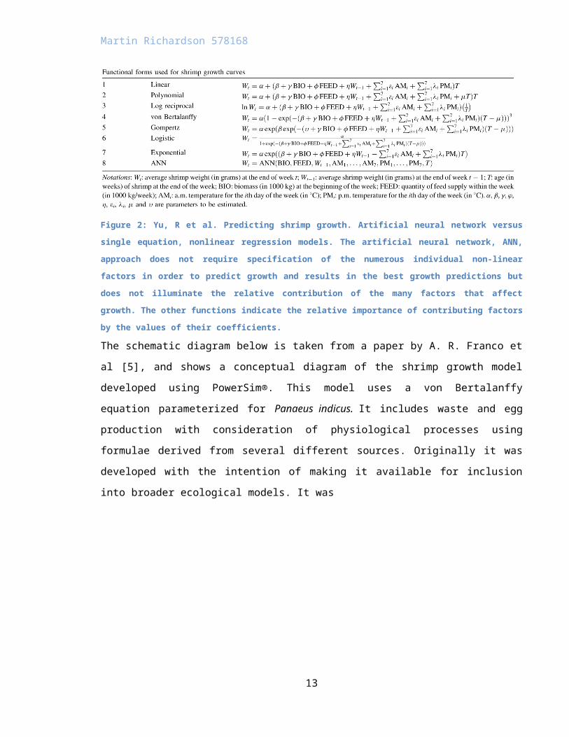
Figure 2: Yu, R et al. Predicting shrimp growth. Artificial neural network versus single equation, nonlinear regression

models. The artificial neural network, ANN, approach does not require specification of the numerous individual non-

linear factors in order to predict growth and results in the best growth predictions but does not illuminate the relative

contribution of the many factors that affect growth. The other functions indicate the relative importance of contributing

factors by the values of their coefficients.

The schematic diagram below is taken from a paper by A. R. Franco et al [5], and shows a conceptual

diagram of the shrimp growth model developed using PowerSim®. This model uses a von Bertalanffy

equation parameterized for Panaeus indicus. It includes waste and egg production with consideration

of physiological processes using formulae derived from several different sources. Originally it was

developed with the intention of making it available for inclusion into broader ecological models. It

was

Figure 3: Franco, A R et al, 2006. Here two forcing functions are considered: food availability and water temperature.

Temperature affects both the feeding rate and metabolism.

10


subsequently updated to include additional factors and incorporated into a commercial software

package called POND for use by shrimp farmers. It can be seen that the POND model incorporates

effects due to temperature, salinity, and dissolved oxygen as well as natural food (zooplankton and

bacteria) which feed on phytoplankton occurring in the water. The model also includes business

planning as well as a cost and profit analysis.

Figure 4: POND® shrimp aquaculture software console.

An additional model derived from fish was produced by Mishra et al. in 2002[15] in attempt to try

and better understand shrimp bioenergetics in order to consider fluctuations in wild populations.

This model details several physiological functions especially relating to metabolism and molting.

Feeding patterns are simulated (nocturnal with cessation during molting) and the discontinuous

growth pattern of shrimp detailed.

11


Figure 5: From Mishra et al. 2002. This model uses results from fish experiments and several assumptions when

experimental data is unavailable.

On a larger scale, models that integrate geographic information from GIS, and hydrodynamic models

to model currents are becoming available. A good example of this is the SMILE project[14][16].

These can be used to evaluate carrying capacity of a coastal area for mariculture of shellfish by

employing an individual species model; in this case it is called SHELLSIM®.

12


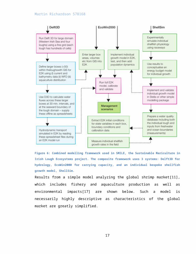
Figure 6: Combined modelling framework used in SMILE, the Sustainable Mariculture in Irish Lough Ecosystems project.

The composite framework uses 3 systems: Delft3D for hydrology, EcoWin2000 for carrying capacity, and an individual

bespoke shellfish growth model, ShellSim.

Results from a simple model analyzing the global shrimp market[11], which includes fishery and

aquaculture production as well as environmental impacts[17] are shown below. Such a model is

necessarily highly descriptive as characteristics of the global market are greatly simplified.

13


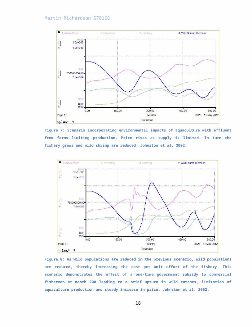
Figure 7: Scenario incorporating environmental impacts of aquaculture with effluent from farms limiting production.

Price rises as supply is limited. In turn the fishery grows and wild shrimp are reduced. Johnston et al. 2002.

Figure 8: As wild populations are reduced in the previous scenario, wild populations are reduced, thereby increasing the

cost per unit effort of the fishery. This scenario demonstrates the effect of a one-time government subsidy to commercial

fisherman at month 200 leading to a brief upturn in wild catches, limitation of aquaculture production and steady

increase in price. Johnston et al. 2002.

Key to model outputs

Actual price Global shrimp price

Harvesting Aquaculture production

14


Catching Fishery production

Wild shrimp biomass

Production of P. Vannamei has undergone a complete shift from wild fishery to aquaculture starting

around the turn of the millennium[18], due in part to development of disease resistant strains[19].

One scenario considered using the model, termed ‘Unbounded Aquaculture’ was closest to the mark

but was not considered a likely outcome. Illustrating how bias can influence the use of a model.

Analysis was skewed towards maintenance of a commercial fishery.

Shrimp characteristics

Penaid shrimp are marine but may spend part of their lifecycle in brackish estuaries [20]. Shrimp live

for 1.5 to 6 years with multiple cohorts in wild populations. In aquaculture there may be more than

one cohort in a pond. As with all crustaceans growth is discontinuous with periods of rapid growth,

no growth, and even negative growth particularly related to water temperature[21]. Growth can be

measured in terms of carapace length, total length or weight. The molt cycle is dependent on the

species in question as well as the age and size of the individual animal. Wild populations synchronize

molting with lunar cycles and bury themselves in the substrate to minimize predation and

cannibalism while the carapace hardens. The molting interval is affected by food availability and

environmental conditions, particular temperature[22]. Molting duration increases as the

temperature drops. Water is taken up during molting, with rapid gain in the wet weight of

replacement exuvia. However, the majority of somatic growth occurs during intermolt periods.

Feeding is nocturnal in many species, and there is a break of several days in feeding while molting

occurs. Feed intake increases with temperature. Light sensitivity to feeding varies widely, with some

species only active for 1 to 2 hours a night[23].

Shrimp show sexual dimorphism with females being larger, and growing faster than males. Females

achieve maturity at approximately 30-40 mm, after some 6 months, and produce from 100,000 to

over 250,000 eggs[23][24]. They usually spawn twice annually, although some species spawn only

once each year. Survivability is related to both temperature and salinity with increased salinity

mitigating against critical low thermal limit associated with mortality. Mortality due to cannibalism,

particularly during molting, is a factor in aquaculture. Aquaculture studies have shown significant

15


increased production potential through the use of a ‘substrate’ made of plastic mesh that permits

vertical separation of the shrimp[25], thereby greatly reducing the effective stocking density.

Methods

Shrimp bioenergetics research by Ingrid Lupatsch et al. at Swansea University’s’ centre for

sustainable aquatic research (CSAR) assessed protein and energy requirements for optimal growth of

shrimp under controlled conditions. Knowing daily protein and energy requirements for provides for

improved aquaculture practice in reducing waste and optimizing feed. Waste from aquaculture

facilities is an important problem[17] and results in contributions to dissolved organic matter as well

as benthic deposits[26]. Feed may account for as much as 50%[27] of all costs. Various protein and

energy sources can be used to formulate a feed to known composition. Until quite recently feed

composition in aquaculture was determined by comparison with dietary requirements of

domesticated animals (e.g. chickens). Since shrimp aquaculture is now a large industrial enterprise

around the World such calculations are of economic importance. For pacific white shrimp (L.

vanneamei) growth was measured by increase in wet weight, the body weight (BW) in grammes at

28°C with 32 ppt (parts per thousand) water salinity. pH and dissolved oxygen (DO) were not

specified. The equation for growth rate applies to post larval juvenile and adult stages over the range

of 1 g to 35 g.

This is an individual growth model so all quantities are per shrimp.

Growth rate is measured as incremental body weight per day, weight gain (g day -1).

(1) Growth rate (g day-1) = 0.050 × BW 0.582 , for 1g ≤ BW ≤35g

(2) Voluntary feed intake rate (g day-1) = 0.086 × BW 0.720

Energy requirements in kJ per day

Digestible energy required for maintenance, DEmaint (kJ day-1)

(3) DEmaint=0.345xBW (kJ day-1)

(4) Expected energy gain (kJ day-1) =(growth rate)x(energy content of gain)

Energy content of gain =4.844 kJ g-1

Energy gain = 0.050 × BW 0.582x4.844 (kJ day-1)

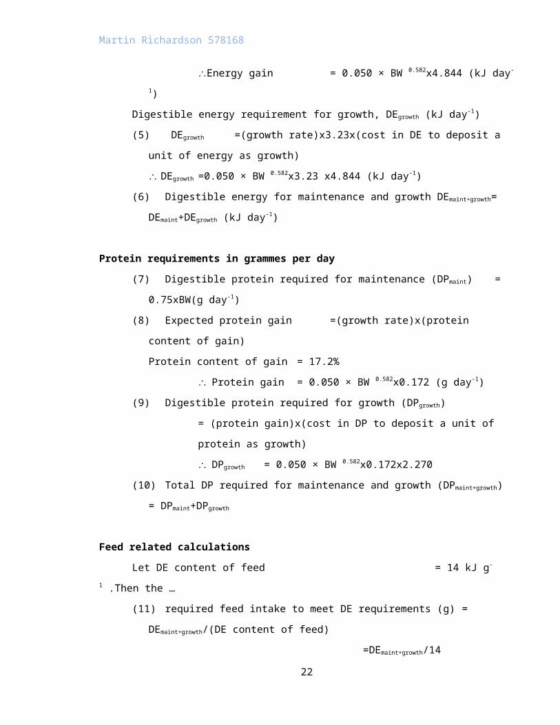
Digestible energy requirement for growth, DEgrowth (kJ day-1)

(5) DEgrowth =(growth rate)x3.23x(cost in DE to deposit a unit of energy as growth)

16


DEgrowth =0.050 × BW 0.582x3.23 x4.844 (kJ day-1)

(6) Digestible energy for maintenance and growth DEmaint+growth= DEmaint+DEgrowth (kJ day-1)

Protein requirements in grammes per day

(7) Digestible protein required for maintenance (DPmaint) = 0.75xBW(g day-1)

(8) Expected protein gain =(growth rate)x(protein content of gain)

Protein content of gain = 17.2%

Protein gain = 0.050 × BW 0.582x0.172 (g day-1)

(9) Digestible protein required for growth (DPgrowth)

= (protein gain)x(cost in DP to deposit a unit of protein as growth)

DPgrowth = 0.050 × BW 0.582x0.172x2.270

(10) Total DP required for maintenance and growth (DPmaint+growth) = DPmaint+DPgrowth

Feed related calculations

Let DE content of feed = 14 kJ g-1 .Then the …

(11)required feed intake to meet DE requirements (g) = DEmaint+growth/(DE content of feed)

=DEmaint+growth/14

(12)Required DP content of feed to meet DP requirement (%)=(DPmaint+growthx100)/Feed intake

=(DPmaint+growthx100)/(DEmaint+growth/14)

=14x100xDPmaint+growth/DEmaint+growth

=1400xDPmaint+growth/ DEmaint+growth

(13)Feed conversion ratio (FCR) =(feed intake)/(weight gain)

(14)DP/DE ratio =DP content of feed (mg)/DE content of feed(kJ)

17


Energy

Total energycomponent

DEmaint

Energy gain

Energy content ofbody

DEgrowth

DEefficiency

Growth Rate

Body Weight

DEmaint&growth

DEcost

Figure 9: Energy component of model. The diamonds are constants. Circles and oblongs are variable quantities that are

calculated using inputs from incoming arrows. The bracketed variables reference the same quantities at different

locations within the model without using connecting arrows and thereby reduce clutter.

Model object name Quantity Value/ Equation number

Energy content of body Constant 4.844 kJ g-1[28]

Total energy component (Energy content of body)x(body weight)

DEmaint DEmaint (3)

DEgrowth DEgrowth (5)

DEmaint&growth DEmaint+growth (6)

Energy gain (4)

DEefficiency Constant 0.31

DEcost 1/DEefficiency 3.23

18


Protein

protein content ofbody

Total proteincomponent

Body Weight

Growth Rate

Protein gain

DPgrowthDPmaint

DPefficiency

DPmaint&growth

DPcost

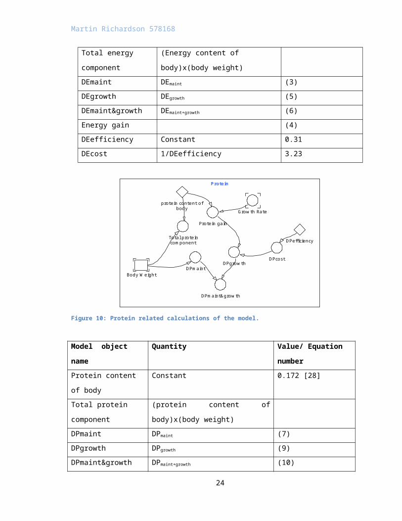
Figure 10: Protein related calculations of the model.


Protein content of body Constant 0.172 [28]

Total protein

component

(protein content of body)x(body weight)

DPmaint DPmaint (7)

DPgrowth DPgrowth (9)

DPmaint&growth DPmaint+growth (10)

Protein gain (8)

DPefficiency Constant 0.44

DPcost 1/DPefficiency 2.27

19

Body WeightGrowth Rate

Voluntary FeedIntake

a

b


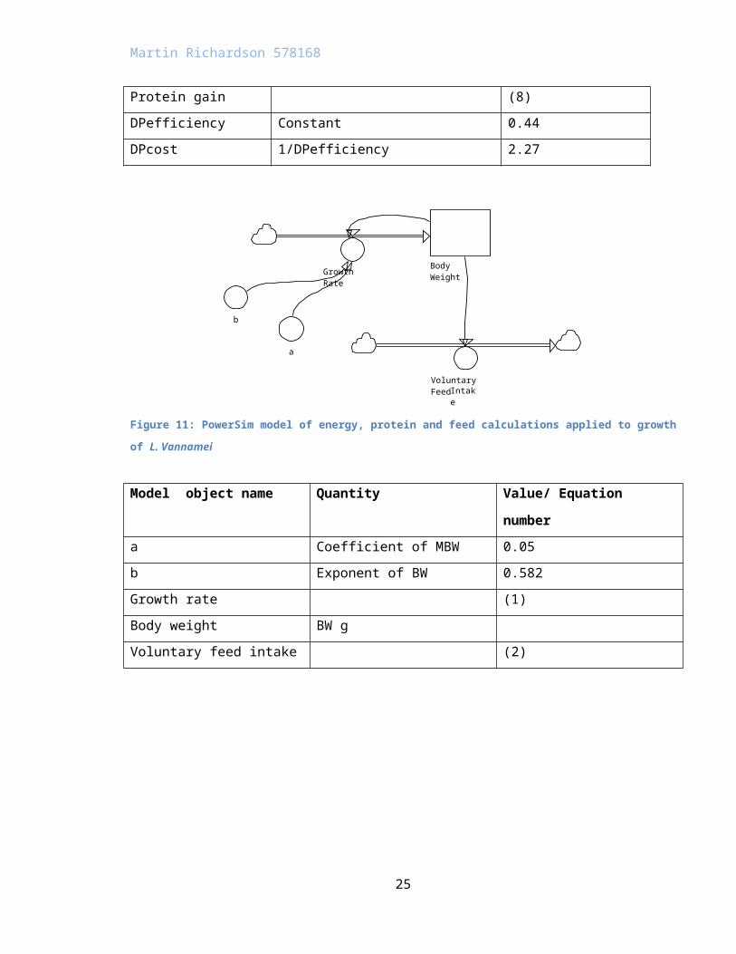
Figure 11: PowerSim model of energy, protein and feed calculations applied to growth of L. Vannamei


a Coefficient of MBW 0.05

b Exponent of BW 0.582

Growth rate (1)

Body weight BW g

Voluntary feed intake (2)

20


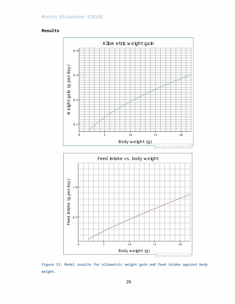
Results

Allometric weight gain

0 5 10 15 20

0.1

0.2

0.3

0.4

Body weight (g)

Wei

ght g

ain

(g p

er d

ay)

Non-commercial use only!

Feed intake vs. body weight

0 5 10 15 20

0.5

1.0

Body weight (g)

Feed

inta

ke (g

per

day

)


Figure 12: Model results for allometric weight gain and feed intake against body weight.

These results match the calculations given in Lupatsch et al. 2008 as listed below.

21


Figure 13: Lupatsch et al. 2008. Studies on Energy and Protein Requirements to Improve Feed Management of the Pacific

White Shrimp, Litopenaeus vannamei. The calculations have been completed for shrimp at 2 different weights: 2g and

10g. Feed calculations follow from specified digestible energy (DE) content which was set at 14 kJ g -1.

22


Growth in L. vannamei at 28 C with 32 ppt salinity andoptimal feeding

0 20 40 60 80 100 120 1400

10

20

30

Time in days

Body

Wei

ght (

g)


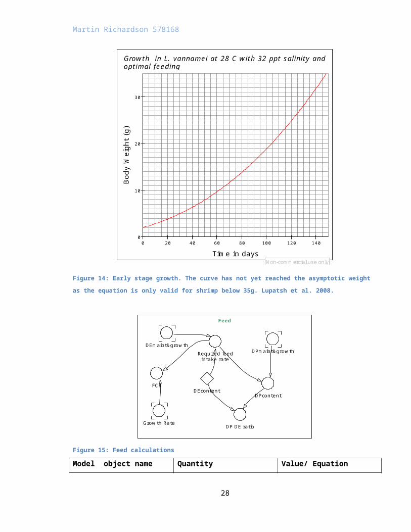
Figure 14: Early stage growth. The curve has not yet reached the asymptotic weight as the equation is only valid for

shrimp below 35g. Lupatsh et al. 2008.

Feed

Required feedintake rate

DEcontent

DEmaint&growth

DPcontent

DPmaint&growth

FCR

Growth Rate DP DE ratio

Figure 15: Feed calculations


DEmaint&growth DEmaint+growth (5)

23


DPmaint&growth DPmaint+growth (9)

Required feed intake rate Required feed intake for growth (10)

DEcontent DE content of feed (constant) 14 kJ g-1

DPcontent Required DP content of feed

(%)

(11)

DP DE ratio DP/DE (13)

FCR Feed conversion ratio (FCR) (12)

0 10 20 30 40 50 60 70 80 90 100 110 120 130 140 150

0.5

1.0

Required feed intake rate Voluntary feed intake

Time in days

Feed

inta

ke in

gra

mm

es


Figure 16: Model results showing voluntary feed intake against actual feed intake.

Discussion

Experimental results for shrimp growth, as well as growth models[5,15,29] all show generally

monotonic, asymptotic curves from juvenile through to adult stage. While there are numerous

factors that affect growth at the individual level, temperature and the molting cycle appear to be

most important. Growth has also been found to be affected by stocking density and biomass as well

24


as water salinity, pH, naturally occurring food[30][31] and photoperiod. There are numerous studies

in the literature addressing one or more of these environmental factors; however no clear picture

emerges as to how they interact to affect growth in combination. The mode developed by Franco et

al. [5] indicates sensitivity to temperature as shown below and this is also evident from experiments

and aquaculture.

Figure 17: Franco, A. R. et al, 2006. The model developed by Franco et al. is not sensitive to a ±10% variation in food

availability, but shows susceptibility to a ±10% change in water temperature indicating that temperature has a major

effect on growth.

Temperature considerations

Wild shrimp populations and pond shrimp are subjected to diurnal and seasonal temperature

variation. The characteristics of these temperature changes are well understood[32]. Seasonal

temperature effects upon growth can be added to the model. Temperature curves are generally

sinusoidal with a winter minimum and summer maximum as shown below.

25


Figure 18: Adamack et al. 2012. Seasonal temperature curve for wild shrimp population.

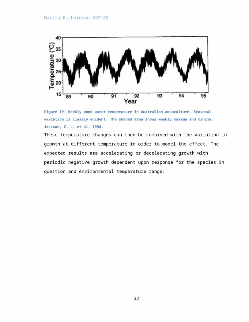
Figure 19: Weekly pond water temperature in Australian aquaculture. Seasonal variation is clearly evident. The shaded

area shows weekly maxima and minima. Jackson, C. J. et al. 1998.

These temperature changes can then be combined with the variation in growth at different

temperature in order to model the effect. The expected results are accelerating or decelerating

26


growth with periodic negative growth dependent upon response for the species in question and

environmental temperature range.

Figure 20: Growth in length at various temperatures. Species not identified. Source: Northern Gulf Institute, data derived

from the literature. Growth ceases at 0°C and increases to a maximum rate at around 25°C. As temperature increases,

growth declines and stops at approximately 35°C. Continuing temperature increases result in mortality. This is a problem

in shallow aquaculture ponds in the tropics. Low temperatures can decimate overwintering stocks in wild shrimp.

Food intake and growth increase with water temperature but decline beyond the optimal point.

Franco et al. [5] used a quadratic equation as a temperature function , f (T ) , to model the effect of

temperature on shrimp feeding rate.

(15)f (T )=−0.02T2+1.44T−17.41R32

[5]

Where R32 is the maximum feeding rate at the optimum temperature of 32°C for P. japonicus. If we

assume that the behavior is similar for P. vannemei, and that the maximum feeding rate is achieved

at, say 27°C then the general form of the graph of this function is as follows:

27


Figure 21: General form of the temperature function with temperature in °C on the x-axis. The y-axis value represents a

growth coefficient, as yet not defined.

Using the graph in figure (18) above taken from Adamack et al. 2012 , the annual temperature

variation in this location (Mississippi, USA) is approximately 22°C over 365 days (1 year). We can

approximate this without considering the actual date using the following equation:

(16)Water temperature=11sin(360 D /365)+24, where D is the time in days.

0 20 40 60 80 100 120 1400

10

20

30

40

Time in days

Wat

er t

empe

ratu

re


Figure 22: Natural fluctuation in water temperature associated with seasonal change over time.

Equation (16) can then be adjusted to match particular dates as required. Further studies, possibly

combined with salinity variation[33], are needed in order to better understand temperature effect. A

study by Rothlisberg, 1998 [34]considered larval growth as illustrated below

28


Figure 23: Rothlisberg, 1998. Effects of salinity and temperature on growth of shrimp protozoae.

Molting

Figure 24: Simulated oxygen consumption during 3 stages of moulting, pre-moult, moult, and post-moult. Mishra et al

2002. In actuality the cycle increases with size and age of the individual.

P. vannamei, molt every 5 days at 1-5g and every 14 days at 15g[23][35]. Information regarding the

molting cycle permits derivation of a scalar quantity that can be used to stretch the timeline, thereby

increasing both the inter-moult period and the length of the molt itself to better match observed

behavior. However, molting is also affected by temperature as shown below. Molting interval

increases inversely with temperature[36][22], tripling as temperature drops from 18°C to 14°C.

29


Figure 25: Molting period at 3 different temperatures. Kumlu et al 2005.

Conclusion

In order to improve the model additional experiments are needed to better understand the effects of

salinity and temperature, molting and spawning. There is little available data in the literature

concerning shrimp bioenergetics in general and environmental effects in particular. There is need to

standardize nomenclature, notation and formulae so as to provide a more rigorous foundation for

this field of research and to avoid errors of interpretation. A standardized metadata and verification

algorithm would also permit easier combination and exchange of models. The primary value is in the

data, as well as associated costs so best practice might involve the sharing of ‘open’ models through

the use of an industry ‘ecosystem’ of stakeholders. This would ensure improved scrutiny of the

methods used and enable the facilitation of popularity ratings and error calculation to indicate

stability as an indication of descriptive vs. quantitative purpose.

Appendix

Body weight to carapace length conversionA body weight to carapace length conversion formula[5] was developed by Franco et al. in their paper ‘Development of a growth model for penaeid shrimp’. Shrimp were measured and weighed to determine the relationship. The species used was Penaeus indicus.

Log10BW = 2.8xLog10CL -2.9

References

30


1 Bureau, D. & Azevedo, P. 2000 Pattern and cost of growth and nutrient deposition in fish and shrimp: Potential implications and applications. , 111-140.

2 Adamack, A., Stow, C., Mason, D., Rozas, L. & Minello, T. 2012 Predicting the effects of freshwater diversions on juvenile brown shrimp growth and production: a Bayesian-based approach. Marine Ecology Progress Series 444, 155-173. (doi:10.3354/meps09431)

3 Lupatsch, I. 2009 Quantifying nutritional requirements in aquaculture: the factorial approach. New Technologies in Aquaculture. Woodhead Publishing Limited, Cambridge, UK , 417–439.

4 Lupatsch, I. In press. Aquatic Animal Nutrition Feed formulation. Growth (Lakeland)

5 Franco, a, Ferreira, J. & Nobre, a 2006 Development of a growth model for penaeid shrimp. Aquaculture 259, 268-277. (doi:10.1016/j.aquaculture.2006.05.051)

6 Daviddottir, B. 2002 Management of the Commons: Social Behavior and Resource Extraction. In Dynamic Modeling for Marine Conservation (eds M. Ruth & J. Lindholm), pp. 356-373. Springer.

7 Kleiber, M. 1932 Body size and metabolism. Hilgardia 6, 37.

8 Green, D. 1976 The historical development of complex numbers. The Mathematical Gazette 60, 99-107.

9 Yu, R., Leung, P. & Bienfang, P. 2006 Predicting shrimp growth: Artificial neural network versus nonlinear regression models. Aquacultural Engineering 34, 26-32. (doi:10.1016/j.aquaeng.2005.03.003)

10 Tetlock, P. 2006 Expert Political Judgment: How Good Is It? How Can We Know? Princeton University Press; New Ed edition (31 July 2006).

11 Johnston, D., Soderquist, C. & Meadows, D. 2002 The Global Shrimp Market. In Dynamic Modeling for Marine Conservation (eds M. Ruth & J. Lindholm), pp. 394-417. Springer New York.

12 Christensen, V. 2009 Ecopath with Ecosim: linking fisheries and ecology. In Handbook of ecological modelling and informatics (eds S. E. Jorgensen T. S. Chon & F. Recknagel), pp. 55-70. WITpress.

13 France, B. 2002 Policy Research for Sustainable Shrimp Farming in Asia Centre for the Law and Economics of the Sea CEDEM University of Shrimp Farming in Thailand : A Review of Issues Shrimp Farming in Thailand : A Review of Issues.

31


14 Ferreira, J. et al. In press. SMILE Sustainable Mariculture in northern Irish Lough Ecosystems.

15 Mishra, A. K., Verdegem, M. & Dam, A. V. 2002 A Dynamic Simulation Model for Growth of Penaeid shrimps. Metabolism Clinical And Experimental

16 Franco, a, Ferreira, J. & Nobre, a 2006 Development of a growth model for penaeid shrimp. Aquaculture 259, 268-277. (doi:10.1016/j.aquaculture.2006.05.051)

17 Cao, L., Wang, W., Yang, Y., Yang, C., Yuan, Z., Xiong, S. & Diana, J. 2007 Environmental impact of aquaculture and countermeasures to aquaculture pollution in China. Environmental science and pollution research international 14, 452-62.

18 Holthius, L. B. 1980 FAO Species Catalogue Shrimps and Prawns of the World.

19 Wyban, J. 2007 Domestication of pacific white shrimp revolutionizes aquaculture. Global Aquaculture Advocate , 3.

20 Padlan, P. G. 1987 Pond culture: Pond Culture of Penaeid Shrimp. UN FAO: Fisheries & Aquaculture department.

21 Coman, G. J., Crocos, P. J., Preston, N. P. & Fielder, D. 2002 The effects of temperature on the growth, survival and biomass of different families of juvenile Penaeus japonicus Bate. Aquaculture 214, 185-199. (doi:10.1016/S0044-8486(02)00361-7)

22 Kumlu, M. & Kir, M. 2005 Food consumption, moulting and survival of Penaeus semisulcatus during over-wintering. Aquaculture Research 36, 137-143. (doi:10.1111/j.1365-2109.2004.01196.x)

23 Dall, W. 1990 The biology of the Penaeidae. Academic Press Limited.

24 2012 Cultured Aquatic Species Information Program Penaeus vannamei. pp. 1-15. UN FAO: Fisheries & Aquaculture department.

25 Tidwell, J. & Coyle, S. 2008 Impact of Substrate Physical Characteristics on Grow Out of Freshwater Prawn, Macrobrachium rosenbergii, in Ponds and Pond Microcosm Tanks. Journal of the World Aquaculture Society 39, 406–413.

26 Jimenez-Montealegre, R., Verdegem, M. C. J., van Dam, A. a & Verreth, J. a 2005 Effect of organic nitrogen and carbon mineralization on sediment organic matter accumulation in fish ponds. Aquaculture Research 36, 1001-1014. (doi:10.1111/j.1365-2109.2005.01307.x)

27 Lupatsch, I. In press. Aquatic Animal Nutrition Feed formulation. Growth (Lakeland)

32


28 Lupatsch, I., Cuthbertson, L., Davies, S. & Shields, R. J. 2008 Studies on Energy and Protein Requirements to Improve Feed Management of the Pacific White Shrimp , Litopenaeus vannamei. Management , 281-295.

29 Jackson, C. 1998 Modelling growth rate of Penaeus monodon Fabricius in intensively managed ponds: effects of temperature, pond age and stocking density. Aquaculture research , 27-36.

30 Wyban, J. A., Lee, C. S., Sato, V. T. & Ssveekey, J. N. 1987 Effect of Stocking Density on Shrimp Growth Rates in Manure-Fertilized Ponds. Public Health 61.

31 Otoshi, C. A., Moss, D. R. & Moss, S. M. 2011 Growth-Enhancing Effect of Pond Water on Four Size Classes of Pacific White Shrimp, Litopenaeus vannamei. Journal of the World Aquaculture Society 42, 417–422.

32 Hoang, T., Lee, S. Y., Keenan, C. P. & Marsden, G. E. 2002 Cold tolerance of the banana prawn Penaeus merguiensis de Man and its growth at different temperatures. , 21-26.

33 Adamack, A. T., Stow, C. A., Mason, D. M., Rozas, L. P. & Minello, T. J. 2009 Temperature and Salinity Effects on the Growth and Survival of Juvenile Penaeid Shrimps: Implications for the Influence of River Diversions on Production.

34 Rothlisberg, P. C. 1998 Aspects of penaeid biology and ecology of relevance to aquaculture: a review. Aquaculture 164, 49-65. (doi:10.1016/S0044-8486(98)00176-8)

35 Nunes, a 2000 Size-related feeding and gastric evacuation measurements for the Southern brown shrimp Penaeus subtilis. Aquaculture 187, 133-151. (doi:10.1016/S0044-8486(99)00386-5)

36 Sarac, H. Z., McMeniman, N. P., Thaggard, H., Gravel, M., Tabrett, S. & Saunders, J. 1994 Relationships between the weight and chemical composition of exuvia and whole body of the black tiger prawn, Penaeus monodon. Aquaculture 119, 249-258. (doi:10.1016/0044-8486(94)90179-1)

33

Documents

Modeling shrimp protein and energy requirements for …€¦ · Web viewModeling shrimp protein and energy ... and other fields such as sociology that now rely on extensive