The Regional Economics Applications Laboratory (REAL) is a unit in the University of Illinois focusing

on the development and use of analytical models for urban and region economic development. The

purpose of the Discussion Papers is to circulate intermediate and final results of this research among

readers within and outside REAL. The opinions and conclusions expressed in the papers are those of the

authors and do not necessarily represent those of the University of Illinois. All requests and comments

should be directed to Geoffrey J.D. Hewings, Director, Regional Economics Applications Laboratory,

607 South Mathews, Urbana, IL, 61801-3671, phone (217) 333-4740, FAX (217) 244-9339.

Web page: www.real.illinois.edu/

Modeling Regional Productive Performance Using a Spatial Stochastic

Frontier Approach: New Evidence for Europe (1995-2007)

Julián Ramajo and Geoffrey J. D. Hewings

REAL 16-T-2 March, 2016

Modeling Regional Productive Performance Using a Spatial Stochastic

Frontier Approach: New Evidence for Europe (1995-2007)

Julián Ramajo

UNIVERSITY OF EXTREMADURA (BADAJOZ, SPAIN)

Geoffrey J.D. Hewings

UNIVERSITY OF ILLINOIS AT URBANA-CHAMPAIGN (URBANA, IL, USA)

Abstract:

The literature on the measurement of regional convergence at different spatial scales and over

different time periods is extensive. This study explores the potential role of variations in

European regional technical efficiency as a contributing factor in providing explanation for

convergence or divergence. To control for spatial dependence among regions, the paper uses a

spatial stochastic frontier approach that integrates spatial econometric techniques with stochastic

frontier models, also allowing for non-linear technical progress jointly with time and cross-

sectional varying technical efficiency. From the estimated production function, we obtain

estimates of the technical efficiency of the investigated 120 NUTS-2 regions of the European

Union over the period 1995-2007. Our findings show that geographical externalities affect the

EU frontier level, and that European regions have been converging to the frontier at a rate of

about 0.8% per year. However, the analyses of the efficiency scores reveal that there is a strong

geographic pattern of regional efficiency while the degree of average regional efficiency has

increased steadily year by year. Overall, it appears that European regions have converged during

the 1995-2007 period in terms of their ability to utilize physical capital and labor to produce

gross value added.

Keywords:

Technical efficiency; spillover effects; frontier analysis; stochastic production function; spatial

panel model; European regions.

1. Introduction

Since Baumol’s (1986) pioneering work, a great number of empirical studies have attempted to

test the hypothesis of regional convergence, according to which poor regions tends to grow faster

than rich regions, such that there exists a process of catching-up of less developed regions with

the richer regions in terms of the level of per capita income (Barro and Sala-i-Martin, 1991).

Following this literature, the primary sources of regional economic growth and development are

centered on two basic explanations, factor accumulation and productivity growth, total factor

productivity (TFP) being considered as the most important driver behind economic growth (e.g.

Caselli, 2005; Parente and Prescott, 2005).

Therefore, proper understanding about how the productivity of regions evolves over time is

essential to an understanding of the current and future trends in regional income levels, and

growth in per capita income. In this sense, as TFP growth is often decomposed (ignoring the

scale component) into technical change (technological innovation) and technical efficiency

(technological catch-up), efficiency is an important component of productivity (Färe et al., 1994;

Kumar and Russell, 2002). Then, the exploration of variations in regional efficiency can provide

new insights in the explanation for convergence or divergence of regions (see Crespo-Cuaresma

et al., 2014, and Piribauer, 2016, for recent empirical studies that analyze regional growth

determinants and income convergence in Europe incorporating model uncertainty and spatial

spillovers simultaneously). Furthermore, because several studies have shown that failure to

account for spatial correlation effects in modeling technical efficiency can result in biased

estimates of efficiency scores (e.g. Schmidt et al., 2009), it is important to use an econometric

framework for accommodating the presence of cross-sectional dependence in the observed

regional production data.

In this context, our paper contributes to the literature on determinants of regional efficiency in

two ways. On the one hand, to the best of our knowledge, this is the first paper that applies

spatial stochastic frontier production functions to analyze technical efficiency of European

regions.1 We explicitly take into account spatial spillover effects by including a spatial lag term

in the econometric frontier specification. While spatial versions of stochastic frontier models

exist (see section 2), they still remain scarce and none concern the issue of regional production

efficiency in Europe. Moreover, by merging techniques used in the stochastic frontier panel

setting with spatial econometric techniques, we have developed two new spatial autoregressive

production frontier panel data models where technical efficiency can be time-invariant or time-

varying, in this last case permitting inefficiency to increase or decrease exponentially depending

1 For non-spatial applications to the European case see, for example, Angeriz et al. (2006), Enflo and Hjertstrand

(2009), or Ezcurra et al. (2008). These three papers address the issue of regional efficiency by means of the

nonparametric Data Envelopment Analysis (DEA).

only on a scalar measuring the yearly rate of technological catch-up. These models extend the

non-spatial estimators proposed by Battese and Coelli (1988, 1992) to the case where there is

spatial dependence in the data.

The rest of the paper is structured as follows. Section 2 reviews the literature of stochastic

frontier models with spatial dependence. The econometric methodology is then discussed in

section 3, followed by the empirical application that contains a discussion of the sample data, the

production function specification, and the main estimation results for production technology

parameters and the efficiency ranking of individual regions. The final section summarizes and

presents conclusions.

2. Frontier models with spatial dependence: A brief review of the literature

After the pioneer spatial autoregressive model by Cliff and Ord (1973), there has developed an

extensive spatial econometrics literature dealing with interactions of economic units in space and

over time (see, for example, the paper of Anselin, 2010, which describe the development of this

field of spatial analysis during the past 30 years; spatial panel data models are discussed in detail

in Baltagi, 2011, 2013, or in Elhorst, 2009, 2014). However, although the economic theory

recognizes that spatial dependency can influence on the productivity of economic units

(Acemoglu, 2009), the field of efficiency analysis generally does not take spatial interaction

effects into account, notwithstanding evidence that efficiency improvements are one of the key

components of productivity growth.

Only recent studies have tried to incorporate spatial dependence into frontier models. As a result,

a new class of spatial frontier models has recently appeared in the productivity and efficiency

analysis literature (see, e.g., Druska and Horrace, 2004; Schmidt et al., 2009; Affuso et al., 2010;

Barrios and Lavado, 2010; Areal et al., 2012; Pavlyuk, 2011, 2012, 2013; Brehm, 2013; Glass et

al., 2013, 2014, 2016; Fusco and Vidoli, 2013; Adetutu et al., 2015; Ramajo et al., 2015; Han et

al., 2016; Mastromarco et al., 2016). We will next briefly review these papers in order to put the

approach proposed in this paper into context.

Druska and Horrace (2004) is the first study in the literature on spatial frontier modeling. The

authors develop a spatial error production frontier panel data model (an extension of the Kelejian

and Prucha’s, 1999 specification for cross-sectional data) which they estimate using the

Generalized Moments method using a sample of Indonesian rice farms, calculating time-

invariant inefficiencies using the Schmidt and Sickles’s (1984) method. They conclude that

spillovers affect farm-level efficiency and ranking.

In Schmidt et al. (2009) a stochastic frontier model with a latent spatial structure is proposed to

account for possible unknown geographical variation of the outputs of farms in Brazil. Their

results demonstrate that models that ignore spatial effects produce significantly different ranking

of inefficiencies across agents than those models that include the latent spatial effects.

In the context of impact evaluation programs that aim to increase efficiency and productivity of

firms in developing countries, Affuso et al. (2010) propose a spatial autoregressive stochastic

production model that estimates the technical efficiencies of matched subsamples of treated and

control farmers in rural areas of Tanzania. Their article extends the literature addressing the

presence of self-selectivity bias considering both the issue of spatial autocorrelation and the

problem of sample selection

Barrios and Lavado (2010) propose an augmented stochastic frontier model that includes a

sparse autoregressive component in the cross-section case, accounting for spatial externalities in

the production capacity of the producers, or a spatial-temporal component for a panel data, where

information on both temporal dependencies and the interaction among units at specific points of

time is present. Using two data sets for Philippines, the authors show that these components can

improve estimates of technical efficiency in a production frontier that is usually biased

downwards.

Areal et al. (2012) incorporate spatial dependence into stochastic frontier analysis using an

autoregressive specification for the inefficiency component of a compound error term, and

employ this method to analyze technical efficiency of a sample of dairy farms in England and

Wales. Their results suggest that there is spatial dependence in technical efficiency in the

analyzed units, and not accounting for it may produce biased results for the efficiency

distribution.

Pavlyuk (2011, 2012, 2013) develops spatial modifications of the standard stochastic frontier

model that include spatial lags, spatial autoregressive disturbances and spatial autoregressive

inefficiencies. Maximum Likelihood (ML) estimators are derived for some of these models, and

small sample properties are investigated with a set of Monte Carlo experiments. Also the ML

estimators are tested with real-world data sets of regional tourism markets in the Baltic States

and of the European airports; in all the empirical applications significant spatial components in

data are discovered. The main conclusion is that non-inclusion of spatial components into

frontier models can lead to significant biases of frontier parameters and efficiency levels

estimates.

Brehm (2013) analyzes the potential link between fiscal decentralization and economic

efficiency for a panel of counties from a Chinese province based on a stochastic frontier model

with spatial error correction. The paper examines in addition the role of an estimation bias due

to spatial and serial correlation. The results point to the significance of the benchmarking or

competition effect, this effect identifying the spatially interdependent allocation of public

investments as a major source for differences in inefficiency at the county level.

Glass et al. (2013, 2014) introduce the concept of efficiency spillover, extending the non-spatial

Cornwell et al.’s (1990) model to the case where there is spatial autoregressive dependence. On

the other hand, Glass et al. (2016) use a composed error structure by assuming a half-normal

distribution for inefficiency. Their approach permits the analyst to benchmark how successful

units are at exporting and importing productive performance to and from other units. Features of

the modeling include time-varying efficiency and estimation of own and spillover returns to

scale. The model is applied to aggregate production in European countries and state-level

manufacturing costs in the US, highlighting in all cases the asymmetry between efficiency

spillovers to and from a decision-making unit.

As in Areal et al. (2012), Fusco and Vidoli (2013) include a spatial lag in the inefficiency term of

the compound error term to allow the splitting of the inefficiency into a spatial component and

into a specific term for every firm. The proposed model is applied to cross-sectional data from

the agricultural sector in Italy. The results show the effectiveness of the proposed technique on

data with uniform and strong spatial dependence, and on data that show only some local

interdependencies.

Adetutu et al. (2015) propose a local spatial stochastic frontier model that accounts for spatial

interaction by allowing spatial lags of the inputs and spatial lags of the exogenous variables to

shift the production frontier technology. Then, the frontier analysis is different from that in

Glass et al. (2013, 2014, 2016), where global spatial dependence is permitted via a spatial lag of

the dependent variable; moreover, rather than calculate efficiency from the cross-sectional

specific effects, they calculate efficiency by making an assumption about the distribution of the

inefficiency component of the error term.

In Ramajo et al. (2015), a nonparametric robust partial frontier methodology is applied to

account for the presence of geographical externalities. Specifically, a spatial autoregressive term

is included as an external factor in a Conditional Order-m model (Cazals et al., 2002; Daraio and

Simar, 2005), permitting the testing of the hypothesis of non-separability (the factor impacts both

the input-output space and the distribution of efficiencies). The results show that geographical

externalities affect both the frontier level and the probability of being more or less efficient.

Specifically, the results support the fact that the spatial autoregressive term has an inverted U-

shaped non-linear impact on the performance of regions.

Han et al. (2016) investigate spillover effects of public capital stock in a production function

model that accounts for spatial dependencies. They use the Schmidt and Sickles’s (1984)

hypothesis of tine-invariant inefficiency, but permit global spatial dependence by introducing a

spatial autoregressive term. Using data for 21 OECD countries from 1960 to 2001, they found

that spillover effects can be an important factor explaining variations in technical inefficiency

across countries as well as discrepancies among various levels of output elasticity of public

capital in traditional production function approaches.

The last contribution in this small body of literature on spatial frontier modeling is Mastromarco

et al. (2016) who proposes a unified framework for accommodating both time and cross-

sectional dependence (strong and weak) in modeling technical efficiency in panel stochastic

frontier models by combining an unobserved common factors-based approach and a threshold

efficiency regime selection mechanism. The proposed approach is applied to a dataset of 26

OECD countries, providing estimation results for the production technology parameters and the

associated efficiency ranking of individual countries. The results show a positive spillover effect

on efficiency, and also permit to identify efficiency clubs endogenously (a technology club, with

countries on or near the frontier, and an inefficiency club, with countries below the frontier).

3. Econometric methodology: Spatial autoregressive stochastic frontier production models

for regional panel data

The aggregate production frontier approach has been used in the cross-country literature to show

that economic growth convergence can be viewed as countries’ movements over time toward the

world or partial-world economy frontiers (efficiency improvements), and to estimate total factor

productivity growth, technical progress, and technological catch-up (see, among others, Kumar

and Russell, 2002; Kneller and Stevens, 2003; Henderson and Russell, 2005; Kumbhakar and

Wang, 2005; Arestis et al., 2006; Henry et al., 2009; Afonso and Aubyn, 2010; ; Growiec, 2012;

Christopoulos and McAdam, 2015).

The production function method has also been used to analyze regional growth in the United

States (e.g., Brock and Ogloblin, 2014) and Europe (e.g., Ezcurra et al., 2008). In this case, the

frontier approach assumes that a region is technically efficient if it produces the maximum

feasible output from a given combination of inputs and technology, regardless of market demand

and prices. On the other hand, it assumes that if a region produces less than is technically

feasible given both technology and inputs, it is inefficient. Hence, inefficiency is measured as

the distance of each individual observation from the frontier.

Following the same methodology of Brock and Ogloblin (2014), in this paper we use the

stochastic production-frontier approach to analyze technical efficiency in European regions.

This method is extended by introducing a spatial autoregressive term to control for spatial

spillover effects that can exist due to cross-regional interdependence. In the next section, we will

outline the proposed spatial stochastic frontier model.

Stochastic production frontier analysis

Aigner et al. (1977) and Meeusen and van den Broeck (1977) pioneered a stochastic production

frontier method to estimate potential output and efficiency characteristics.2 In stochastic frontier

analysis (SFA), a production econometric specification is proposed as:

(1) 𝑌𝑖 = 𝐹(�̃�𝑖, 𝜷)𝑒𝜈𝑖𝑇𝐸𝑖

where Y denotes observed output, 𝑌𝑖∗ = 𝐹(�̃�𝑖, 𝜷) represents the maximum quantity of output that

can be produced from a given K-dimensional input bundle �̃� = (𝑋1, 𝑋2, … , 𝑋𝐾), 𝜷 is the vector of

2 Greene (2008) provides excellent discussions of the development of the field.

parameters of the production function to be estimated, 𝜈𝑖 is a stochastic disturbance term allowing

for unobserved random errors affecting the frontier (exogenous production shocks), and 0 <

𝑇𝐸𝑖 = 𝑌𝑖 𝑌𝑖∗⁄ = 𝑒−𝑢𝑖 ≤ 1 is the Farrell (output oriented) measure of technical efficiency, 𝑢𝑖 ≥ 0

being a measure of the degree of inefficiency in the resource allocation in economic unit i.

The reformulated stochastic frontier (SF) log production model is given by:

(2) log 𝑌𝑖 = 𝑓(�̃�𝑖, 𝜷) +𝜈𝑖 −𝑢𝑖

and then the stochastic frontier is given by 𝑓(�̃�𝑖, 𝜷) +𝜈𝑖 , and 𝑢𝑖 represents the inefficiency

component (see figure 1).

[insert figure 1 about here]

Spatial versions of the cross-sectional SF model (SpSF models)

Using a log-linear functional form approximation for the function f (the log of the production

function F) the standard SF model can be written as:

(3) 𝑦𝑖 = 𝐱𝑖′𝜷 +𝜈𝑖 −𝑢𝑖

where 𝑦𝑖 represents the logarithm of the output of region i, and 𝐱𝑖 is a 𝐾 × 1 vector containing

the logarithms of the inputs (and possibly high-order transformations of them, squared and cross-

product terms). Note that this model does not include any type of spatial dependence, a

potentially restrictive specification in empirical applications where geo-referenced data are used

because there is a high probability that these types of data show some form of spatial

autocorrelation.

Expressing the aspatial SF model 𝑦𝑖 = 𝐱𝑖′𝜷 +𝜈𝑖 −𝑢𝑖 in matrix form,

(4) 𝒚 = 𝐗𝜷 +𝝂 − 𝒖

Pavlyuk (2011, 2012, 2013) proposes a general spatial frontier model for cross-section data

defined by the following equations:3

3 The terms between brackets in equation (5) are not proposed in the original papers of Pavlyuk but we introduced

them following earlier literature modeling inefficiency in terms of exogenous determinants and their spatially lagged

values (see Section 2).

(5)

𝒚 = 𝜌𝐖1𝒚 + 𝐗𝜷 +(𝐖2𝐗)𝜸 + 𝜺𝜺 = 𝝂 − 𝒖

𝝂 = 𝜉𝐖3𝝂 + �̃�

𝒖 = 휂𝐖4𝒖 + [𝐙𝜹 + (𝐖5𝐙)𝝎] + �̃� , 𝒖 ≥ 𝟎

where 𝐖𝑗 are spatial weights matrices with rows 𝐰𝑗,𝑖 specifying the spatial connections of each

unit i according to some measure of proximity between the units. This general unrestricted

specification, introducing spatial lags of the inputs-output vectors, spatial errors, and spatial

inefficiency terms, is a very flexible specification but raises computational problems due to

identification problems. This is the reason because finally only two spatial stochastic frontier

models are considered in the applications, a spatial autoregressive one and a spatial

autoregressive model with spatial autoregressive disturbances.

Panel versions of SpSF models

The frontier models we have discussed to this point have been mainly applied for analysis of

cross-sectional data. Since our application uses a panel of European regions, we need to re-adapt

the above formulation for the case of panel data. The fundamental challenge is to relax some of

the assumptions that the cross-sectional SF model imposes, basically considering a realistic

characterization of the evolution of inefficiencies over time (see Kumbhakar et al., 2014, for a

recent review of competing non-spatial panel data frontier models).

In a non-spatial context, Battese and Coelli (1988) (BC88) extended model (3) to panel data,

proposing the following SF model:

(6)

𝑦𝑖𝑡 = 𝐱𝑖𝑡′ 𝜷 +휀𝑖𝑡

휀𝑖𝑡 = 𝜈𝑖𝑡 − 𝑢𝑖

𝜈𝑖𝑡~𝑁(0, 𝜎𝜈2)

𝑢𝑖~𝑁+(𝜇, 𝜎𝑢2)

This formulation assumes that the (time-invariant) inefficiency term follows a non-negative

truncated-normal distribution that is truncated at zero with mean 𝜇 and variance 𝜎𝑢2 , and the

idiosyncratic error follows a standard symmetric normal distribution 𝜈𝑖𝑡~𝑁(0, 𝜎𝜈2).

Battese and Coelli (1992) (BC92) proposed an alternative (also non-spatial) model with unit-

specific time-varying decay pattern of variation of inefficiency:

(7)

𝑦𝑖𝑡 = 𝐱𝑖𝑡′ 𝜷 +휀𝑖𝑡

휀𝑖𝑡 = 𝜈𝑖𝑡 − 𝑢𝑖𝑡

𝜈𝑖𝑡~𝑁(0, 𝜎𝜈2)

𝑢𝑖𝑡 = ℎ(𝑡)𝑢𝑖

where ℎ(∙) is the deterministic function exp(−휂(𝑡 − 𝑇)) and 𝑢𝑖 is a non-negative truncated-

normal distribution given by 𝑢𝑖~𝑁+(𝜇, 𝜎𝑢2) .

4 When 휂 = 0 , the model BC92 (time-varying

decay) reduces to the model BC88 (time-invariant).

We extend the non-spatial BC88 and BC92 models by generalizing their respective panel

specifications following the same approach used by Pavlyuk (2011, 2012, 2013) for the cross-

sectional case. In particular, a first-order spatial autoregressive -SAR(1) - term have been added

to models (6) and (7) allowing for the existence of substantive spatial autocorrelation between

neighboring units.5 Hence, it is now possible to obtain spatial lag frontier models as follows:

(8)

𝑦𝑖𝑡 = 𝜌𝐰𝑖′𝒚𝒕 + 𝐱𝑖𝑡

′ 𝜷 +휀𝑖𝑡

휀𝑖𝑡 = 𝜈𝑖𝑡 − 𝑢𝑖

𝜈𝑖𝑡~𝑁(0, 𝜎𝜈2)

𝑢𝑖~𝑁+(0, 𝜎𝑢2)

for the BC88 case, and

(9)

𝑦𝑖𝑡 = 𝜌𝐰𝑖′𝒚𝒕 + 𝐱𝑖𝑡

′ 𝜷 +휀𝑖𝑡

휀𝑖𝑡 = 𝜈𝑖𝑡 − 𝑢𝑖𝑡

𝜈𝑖𝑡~𝑁(0, 𝜎𝜈2)

𝑢𝑖𝑡 = exp(−휂(𝑡 − 𝑇)) 𝑢𝑖 , 𝑢𝑖~𝑁+(𝜇, 𝜎𝑢2)

for the BC92 model, where the vectors 𝐰𝑖 of known positive constants specify the strength of the

spatial connections of each unit i according to some measure of proximity between the economic

units, and 𝜌 is the spatial autoregressive parameter.

4 Feng and Serletis (2009) have extended the BC formulation by specifying ℎ(𝑡) = exp(−휂1(𝑡 − 𝑇) − 휂2(𝑡 − 𝑇)2)

in a cost function context. In the same way, Kumbhakar (1991) proposes the function (1 + exp(𝛾1𝑡 + 𝛾2𝑡2))−1 that

can be monotonically increasing (decreasing) or concave (convex). On the other hand, Cornwell et al. (1990)

proposes an alternative model that assumes 𝑢𝑖𝑡 = 𝜔1𝑖 + 𝜔2𝑖𝑡 + 𝜔3𝑖𝑡2 allowing a unit-specific temporal pattern of

inefficiency but requiring the estimation of a large number of parameters. Glass et al. (2013, 2014) have adapted this

last model for the spatial panel data case. 5 Because in our application we are more interested to measure the spillover effects between regions, we only

introduce a spatial autoregressive term but we do not model spatial dependence in the error process 𝜈𝑖𝑡 (as in Druska

and Horrace, 2004). The consideration of a mixed regressive spatial autoregressive specification will be the

objective of future research.

Both models will be the basis for the empirical application presented in the next section. The

main difference between them centers on the hypothesis of time-invariance of technical

efficiency in model (8), which can be tested through the statistical significance of the decay

parameter 휂 in the exponential function of model (9). If the null hypothesis is rejected, technical

efficiency of regions can increase or decrease exponentially depending of the sign of the decay

parameter 휂: when 휂 > 0, this implies that the degree of inefficiency decreases over time, and

units move towards the frontier (technological catch-up) at a rate of (100 × 휂)% per year; if

휂 < 0 , technical inefficiency increases exponentially and this implies divergence (technical

inefficiency is growing).

Comparing the second proposed model with earlier contributions in the spatial stochastic frontier

literature (see section 2), our proposal represents an alternative to other specifications that allows

efficiency to vary over time and over the cross-section. Hence, rather than assume cross-

sectional specific effects in a SAR stochastic frontier model (Glass et al., 2013, 2014), or that the

inefficiency distribution is half-normal (Glass et al., 2016), we use a time-varying decay

efficiency specification.

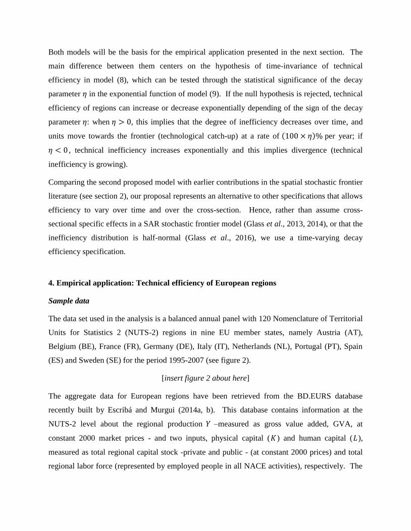
4. Empirical application: Technical efficiency of European regions

Sample data

The data set used in the analysis is a balanced annual panel with 120 Nomenclature of Territorial

Units for Statistics 2 (NUTS-2) regions in nine EU member states, namely Austria (AT),

Belgium (BE), France (FR), Germany (DE), Italy (IT), Netherlands (NL), Portugal (PT), Spain

(ES) and Sweden (SE) for the period 1995-2007 (see figure 2).

[insert figure 2 about here]

The aggregate data for European regions have been retrieved from the BD.EURS database

recently built by Escribá and Murgui (2014a, b). This database contains information at the

NUTS-2 level about the regional production 𝑌 –measured as gross value added, GVA, at

constant 2000 market prices - and two inputs, physical capital (𝐾 ) and human capital (𝐿),

measured as total regional capital stock -private and public - (at constant 2000 prices) and total

regional labor force (represented by employed people in all NACE activities), respectively. The

BD.EURS regional database has been built using information about gross value added, gross

fixed capital formation and employment from three different sources: REGIO-EUROSTAT for

the regional information, and AMECO and EU-KLEMS for the national sources.6

Econometric model specification

We start the empirical analysis by hypothesizing the existence of a regional Cliff-Ord-type

production frontier function which include a variable capturing the interaction between economic

units (the spatial lag of the neighbor’s output): 7

(10) 𝑌𝑖𝑡 = 𝐹 (∑ 𝑤𝑖𝑗𝑌𝑗𝑡

𝑁

𝑗=1

, 𝐾𝑖𝑡, 𝐿𝑖𝑡) 𝑒𝑔(𝑡)𝑒𝜈𝑖𝑡𝑒−𝑢𝑖𝑡

where Y denotes output, K, L represent physical capital and labor respectively, F and g represent

the production and technical progress functions, and subscripts i=1,2,…N and t=1,2,…T

respectively index region and time.

In our application, because of its higher flexibility with respect to the Cobb–Douglas production

function widely used in the related literature, we consider that the functional form for the (log)

production function takes the form of a spatially-augmented translog functional form in terms of

the logarithms of K and L (Christensen et al., 1973);8 in addition, we consider that the technical

progress function can be a non-linear function of a time trend variable. Hence, the SAR(1)

stochastic frontier model is specified as follows:9

6 See Escribá and Murgui (2014b) for details and descriptive statistics of the variables.

7 The corresponding spatial autoregressive parameter, measuring the relevance of spillovers across cross-sectional

units, indicates the direction of the global spatial externalities that the data show (Anselin, 2003): greater this

parameter –in absolute terms- much more the output of each economic unit will depends on the output of its

neighbors. 8 As a robustness exercise we also consider a Fourier functional form that adds trigonometric terms of re-scaled

values of the original variables to the translog production function in order to achieve a more global approximation

to the true frontier (Gallant, 1981, 1982). The efficiency estimates were very similar to the translog case so we omit

these complementary results. 9 As we are aware that subject-specific effects are an important source of heterogeneity in stochastic frontier models

(Greene, 2002, 2005; Chen et al., 2014), we also estimated a country fixed-effects frontier model changing the

constant intercept 𝛼0 by country-specific intercepts, 𝛼0 + 𝐜𝑖′𝜶, where 𝐜

is a vector of dummy variables for eight of

the nine EU countries which regions belong (Germany was used as the base country). This variant yielded similar

estimation results to the obtained with the base model and is not presented here. More general specifications that

include economic, political of socio-cultural indicators of regions have not been estimated due to information

(11)

𝑦𝑖𝑡 = 𝛼0 + 𝜌 ∑ 𝑤𝑖𝑗𝑦𝑗𝑡

𝑁

𝑗=1

+ 𝛽1𝑘𝑖𝑡 + 𝛽2𝑙𝑖𝑡 + 𝛽3𝑘𝑖𝑡2 + 𝛽4𝑙𝑖𝑡

2 + 𝛽5𝑘𝑖𝑡𝑙𝑖𝑡 + 𝛿1𝑡 + 𝛿2𝑡2 + 𝜈𝑖𝑡 − 𝑢𝑖𝑡

where 𝑦𝑖𝑡 , 𝑘𝑖𝑡 and 𝑙𝑖𝑡 are the log of the output, the physical capital, and the human capital,

respectively; t is a time trend; the stochastic noise component 𝜈𝑖𝑡 it is a idiosyncratic term

assumed to be i.i.d. normal with zero mean and constant variance, 𝜈𝑖𝑡~𝑁(0, 𝜎𝜈2), to allow for

unobserved random errors affecting the frontier; and 𝑢𝑖𝑡 represents inefficiency.

For each region, the endogenous spatial lags of the dependent variable are built as ∑ 𝑤𝑖𝑗𝑁𝑗=1 𝑦𝑗𝑡,

with elements 𝑤𝑖𝑗 reflecting the spatial connectivity structure between regions and the strength

of the relationships across them, and satisfying the restrictions 𝑤𝑖𝑗 ≥ 0, 𝑤𝑖𝑖 = 0 and ∑ 𝑤𝑖𝑗𝑁𝑗=1 =

1. In our case, the weights matrix 𝐖 is the row-standardized version of the geographic weight

matrix 𝐂𝑑 in which elements 𝑐𝑖𝑗 have been defined based on inverse distances with a decay

factor 𝑐𝑖𝑗 =1

𝑑𝑖𝑗𝜙 where 𝑑𝑖𝑗 denotes the physical distance between regions i and j, and 𝜙 is the

distance decay parameter. Although 𝜙 can be estimated by nonlinear estimation techniques, we

have used particular values as usual in the literature (see, for example, Crespo-Cuaresma et al.,

2014, Glass et al., 2016). Specifically, we used alternative values 𝜙 = 1 and 𝜙 = 2, and the

results were very similar. This is the reason because from now on we will present the empirical

results using 𝜙 = 1, that to say, we will use in the calculations the inverse distance specification,

𝑐𝑖𝑗 =1

𝑑𝑖𝑗 , and the corresponding row-normalized exogenous, symmetric and dense spatial

weights matrix 𝐖.

The proposed empirical frontier model also allows cross-section heterogeneous inefficiency

terms 𝑢𝑖𝑡 ≥ 0. In our application, two models have been estimated depending of the properties

assumed for the technical inefficiency term:

- Case 1 (Time-invariant inefficiency): 𝑢𝑖𝑡 = 𝑢𝑖~𝑁+(𝜇, 𝜎𝑢2) is a non-negative stochastic term

measuring the distance from the frontier for each region, and following a truncated-normal

distribution (Battese and Coelli, 1988).

restrictions of our database. The specification of a general region-specific fixed or random effects frontier model that

allows time-invariant heterogeneity in the frontier production function will be an area of future research.

- Case 2 (Time-varying inefficiency): 𝑢𝑖𝑡 = ℎ(𝑡)𝑢𝑖, where ℎ(𝑡) = exp(−휂(𝑡 − 𝑇)) and 𝑢𝑖 is a

non-negative stochastic term given by 𝑢𝑖~𝑁+(𝜇, 𝜎𝑢2) (Battese and Coelli, 1992).

10

Both formulated models, containing spatial interaction effects, non-linear technical progress and

heterogeneous time-varying technical efficiency, have been estimated using the Maximum

Likelihood (ML) method taking into account the endogeneity of the spatial lag variable, and the

efficiency estimation procedure involves three sequential steps: in the first step, the parameters

of the frontier model were estimated maximizing the log-likelihood function; after that, point

estimates of inefficiency were obtained through the usual conditional expectation method,

�̂�𝑖𝑡 = 𝐸[𝑢𝑖𝑡|휀𝑖𝑡] (Jondrow et al., 1982); finally, consistent estimates for the technical efficiency

of the ith

region at time t were calculated as τ̂𝑖𝑡 = exp(−�̂�𝑖𝑡).

Discussion of the stochastic frontier and efficiency results

In this section, we focus on the issue of the productive performance of 120 NUTS-2 regions in

nine European countries over the period 1995-2007. In a cross-regional framework, production

inefficiencies can be identified as the distance of the individual region’s production from the

frontier. Hence, efficiency improvement will represent productivity catch-up via technology

diffusion because inefficiencies can reflect a sluggish adoption of new technologies (Ahn and

Sickles 2000).

Productivity catching-up among European regions has been an important topic of interest for

many researchers (e.g. Gardiner et al., 2004, Ezcurra et al., 2007). In particular, it is important

to see how the productivity of European regions evolves over time because the literature

indicates that regional differences in productivity are the main reason for regional growth and per

capita income inequality in the EU (e.g. López-Bazo et al., 1999, Cuadrado-Roura et al., 2000).

In this sense, figure 3 presents the quantile maps of output per worker in 1995 and 2007 obtained

from our database, based on the associated Moran’s scatterplots, and figure 4 presents the usual

absolute β-convergence graph (first panel) for the labor productivity variable –labor productivity

10

In the present version of the paper a constant mean and variance of the distribution of the inefficiency term is

assumed. This limitation would be avoided specifying the mean and the variance as a function of vectors of time-

invariant covariates (or the means of time-varying covariates for each region) as 𝜇𝑖 = 𝛿0 + 휁𝐰𝑖′𝒖 + 𝐳𝑚,𝑖

′ 𝜹 and

𝜎𝑢,𝑖2 = 𝑒𝑥𝑝(𝜔0 + 𝐳𝑣,𝑖

′ 𝝎). Consideration of these extensions will be the immediate objective of future research.

growth 1995-2007 [y-axis] versus labor productivity in 1995 [x-axis]- and the Theil’s inequality

index for this variable over the complete period 1995-2007 (second panel).11

The maps in figure 3 show a strong geographic pattern in the European regional data about

output per worker12

(the values of the Moran’s I statistics reveal the existence of a strong positive

and statistically significant degree of spatial dependence in the distribution of European

productivity), and also suggest the presence of spatial heterogeneity in the form of two spatial

clusters of high and low productive regions: the high-productivity cluster situated in Europe’s

economic core area, the “Blue-Banana” zone (Brunet, 2002; Hospers, 2002), from the West of

England in the north to North of Italy in the south; and the low-productivity cluster including

some of the least developed region or Europe (located in Portugal, Spain, Southern Italy and

Eastern Germany).

The graphs in figure 4 shows that there has been unconditional β-convergence in labor

productivity (the slope of the regression was negative and statistically significant), and that

regional inequality in productivity decreased between 1995 and 2007. Indeed, the index values

fell over 8.5 percent over the thirteen years considered although, as can be seen, the reduction

has not been uniform throughout the period (the main decrease take place in the late nineties and

the early twentieth century).

[insert figures 3 and 4 here]

On the other hand, because productivity growth is the net change in output due to changes in

efficiency and technical change, efficiency is a component of productivity. In fact, the results in

Ezcurra and Iráizoz (2009) show that regional differences in the levels of technical efficiency

account for a relatively important portion of spatial inequality in labor productivity within the

EU. Then, it is a relevant question to analyze the degree of efficiency with which the European

regions use its available resources in production.

Following the spatial stochastic frontier analysis presented in section 3, now we will present the

efficiency estimates obtained for the EU regional panel database used in this work. However,

11

We used the measure of inequality proposed by Theil (1967), 𝑇0(𝑆𝑡) = ∑ 𝑓𝑖𝑡log (𝜇𝑡

𝑆𝑖𝑡)𝑛

𝑖=1 , where 𝑓𝑖𝑡 is the share in

total production of region i, 𝑆𝑖𝑡 is the value of the analyzed variable, S, in region i, and 𝜇𝑡 stands for the weighted

average of the variable S over space, all variables measured at time t. 12

Investigating the sources of regional growth in Europe, López-Bazo et al. (2004) showed that regional

productivity spillovers are far from negligible, and may cause non-decreasing returns at the spatial aggregate level.

before analyzing the efficiency results, we will present and discuss the econometric results for

the selected frontier models. In table 1, we present the maximum-likelihood estimates obtained

for the spatial stochastic frontier models defined by equations (8) and (9) using the production

function given by (11).

[insert table 1 here]

We first have tested the null hypothesis about inefficiency change over time, H0: {휂 = 0} vs.

H1: {휂 ≠ 0}. The null hypothesis was clearly rejected (p-value=0.0000), and the estimate of 휂,

0.008, implies technological catch-up: European regions have been converging to the frontier at

a rate of 0.8% per year, meaning that technical inefficiency has been shrinking at 0.8 percent

points per year.13

Due to the significance of the estimated of 휂, from now on we will only

consider in our analysis the Case 2 of our econometric specification, that is to say, the time-

varying inefficiency production frontier model (column 3 in table 1).

Secondly, with respect to the spatial autoregressive parameter (𝜌), the obtained estimate (0.35) is

positive and statistically significant at much more than 1% level (p-value=0.0000), indicating the

relevance of externalities (such as technological interregional spillovers or factor mobility) in

order to explain the productive process of each region. On the other hand, the estimates of 𝜌

from the Case 1 and Case 2 models are of similar order of magnitude, which indicates that the

degree of global spatial dependence of regional output (𝑦) is robust to the specification of the

technical inefficiency term.14

Finally, all the parameters of the translog function (𝛽’s) and also the trend parameters (𝛿’s) are

statistically significant at more that the 1% level (in all cases the p-value equals 0.0000).

Moreover, the Cobb-Douglas production specification (which impose the restrictions 𝛽3 = 0,

𝛽4 = 0, and 𝛽5 = 0 on equation 12) was clearly rejected by the data (p-value=0.0000). On the

other hand, the statistical significance of the 𝛿’s indicates that the production frontier shifted

appreciably over the considered period according to the values of the estimated parameters, 𝛿1 =

−0.011, and 𝛿2 = 0.0002.

13

Our estimate contrasts with the value of 2.4% obtained by Kumbhakar and Wang (2005) using a non-spatial

stochastic production model for a sample of 82 countries over the period 1960-1987. 14

This result is similar to that obtained by Glass et al. (2016) using aggregate data for 41 European countries for the

period 1990-2011, and several spatial stochastic frontier specifications.

Now we turn to analyzing the efficiency results. First, in table 2 we present the summary

statistics of the regional technical efficiency estimates over the full sample (EU-9 1995-2007),

over space (mean values of efficiency for each country over the whole sample period), and over

time (year by year from 1995 to 2007).15

Figure 5 presents the kernel density distribution of the

estimates over the full sample (1,560 observations), and figure 6 shows the mean (first panel),

and the median, 0.25 and 0.75 quantile scores per year (second panel), this second graph

revealing the spread of the efficiency values, measured by the inter-quantile range.

[insert table 2 here]

[insert figures 5 and 6 here]

Looking at second line of table 2, we can observe that full sample average technical efficiency is

around 0.68, this value implying that the average EU-9 regional efficiency could be increased by

32% if inputs were used in their most efficient combination. On the other hand, the graph in

figure 5 suggests the possibility of uni-modality in the distribution of the full sample technical

efficiency estimates. In fact, the Silverman nonparametric test for multimodality (Silverman,

1981) was applied and the null of uni-modality was not rejected (p-value=0.96). Hence, our

results suggest that there has not been polarization across European regions in terms of technical

efficiency. In other words, there are no spatial convergence clubs in the distribution of technical

efficiency of the European regions.

Additionally, with the “over space” country information contained in table 2 it is possible to

categorize the EU-9 countries in terms of their estimated 1995-2007 average values of technical

efficiency: Austria, Germany and Portugal present values below the EU-9 mean (0.68); Spain,

France, Italy, Netherlands and Sweden show values clustered around the average; and, finally,

only Belgium exhibits a value (0.75) clearly above the EU-9 mean.16

Finally, the “over time” numerical information of table 2, with the graphs contained in figure 6,

show that the degree of average regional efficiency has increased steadily year by year. Overall,

this result shows that European regions have converged during the 1995-2007 period in terms of

their ability to utilize physical capital and labor to produce GVA.

15

Detailed results for individual efficiency for the 120 EU-9 regions can be obtained from the authors upon request. 16

Our mean-country results can be compared with those obtained by Mastromarco et al. (2013) by combining a

dynamic efficiency analysis in the stochastic frontier framework, using a dataset of 18 EU countries over 1970-2004

(see table 3, where efficiency results are showed over the two sub-periods 1970-1995 and 1996-2004)

Figure 7 presents the histogram of the mean regional efficiency scores (averaged for the 1995 to

2007 period) of individual regions, showing the frequency distribution of the estimations.

Additionally, figures 8 and 9 show, respectively, the quantile map of the regional scores (dark-

shaded regions can be considered as comparatively more efficient than light-shaded regions) and

the associated Moran’s scatterplot and I statistic, and the LISA maps (Anselin, 1995) of regional

technical efficiency mean estimations.

[insert figures 7, 8 and 9 here]

Looking at figure 8, the quantile map points to a significant positive spatial dependency between

the efficiency level of each region and the performance of their neighboring regions. This

hypothesis is confirmed by the Moran’s I statistic (I=0.2055), which indicates the presence of a

strong geographic pattern (p-value=0.001). Moreover, the LISA maps of the EU-9 regional

mean efficiency scores of figure 9 show that there are two spatial clusters of European regions:

the first cluster (red color) is characterized by high annual average scores (more efficient

regions) surrounded by regions with similar results (high-high zone in the terminology of the

spatial econometrics literature); the second cluster (blue color) includes more inefficient regions

(low-low zone).

Finally, in order to explore the relative contribution of the technical efficiency component

(change of the obtained efficiency scores) to labor productivity growth, figure 10 presents the

regression line graph between these variables. The corresponding slope coefficient is positive

and statistically significant (p-value=0.0077), which is an indication that a non-negligible part of

European regional productivity growth 1995-2007 can be attributed to changes in technical

efficiency.

6. Final remarks and conclusions

Trying to explore the potential role of variations in regional technical efficiency as a contributing

factor in providing explanation for convergence or divergence in Europe, our paper estimates a

spatial stochastic frontier model that captures global spillovers through the introduction of a

spatial autoregressive term in the assumed translog production technology. Since the spatial

frontier model is applied to an aggregate production function using balanced panel dataset of 120

European regions (in 9 EU member states) over the period 1995-2007, we propose a panel

stochastic frontier model that allows the efficiency effects to vary over time and between cross-

sectional units, also allowing for non-linear exogenous technological change. Specifically, we

have ‘spatialized’ the BC (1992) model, which involves using an inefficiency term with time-

varying factor and time-invariant characteristics (the special case of time-invariant factor

produce the non-spatial BC model, 1988). The derived global spatial stochastic frontier model is

estimated using maximum likelihood methods taking into account the endogeneity of the spatial

lag variable included in the econometric specification.

Using the European regional dataset, we provide satisfactory estimation results for the

production technology parameters, the inefficiency time-varying factor, and the associated

technical efficiency scores of individual regions. We find statistically significant and positive

global spillover effects, showing that geographical externalities affect the EU frontier and

therefore play an important role in regional growth and convergence in Europe, and also we find

that regions have been converging to the EU-9 technology frontier at a statistically significant

rate of 0.8% per year.

Furthermore, our descriptive analysis of the technical efficiencies reveals cross-sectional

dependence in the estimated scores, showing the dependency of a region’s efficiency with the

performance of its neighbors. This finding suggests two areas for future work: to extend the

spatial stochastic frontier models formulated in this paper (which can only accommodate the

weak form of spatial dependence) for more general specifications which can generate strong

and/or weak forms of cross-sectional dependence endogenously, for example following the

approach proposed by Mastromarco et al. (2016) for modeling the time-varying inefficiency

term; to estimate efficiency spillovers to and form a region explicitly, for example using the

method proposed by Glass et al. (2016) to calculate time-varying relative direct, relative indirect

and relative total efficiencies in order to analyze spatial efficiency.

REFERENCES

Acemoglu, D. 2009. Introduction to Modern Economic Growth. Princeton University Press,

Oxford.

Adetutu, M., Glass, A.J., Kenjegalieva, K., and R.C. Sickles. 2015. The effects of efficiency and

TFP growth on pollution in Europe: a multistage spatial analysis. Journal of Productivity

Analysis 43 (3): 307–326.

Affuso, E. 2010. Spatial Autoregressive Stochastic Frontier Analysis: An Application to an

Impact Evaluation Study. Available at SSRN: http://ssrn.com/abstract=1740382.

Afonso, A., and M.St. Aubyn. 2010. Public and private inputs in aggregate production and

growth: A cross-county efficiency approach. Working Paper Series No. 1154, European Central

Bank (ECB), Germany. Available at SSRN: http://ssrn.com/abstract=1551199.

Ahn, S. C., and R.C. Sickles. 2000. Estimation of long-run inefficiency levels: A dynamic

frontier approach, Econometric Reviews 19: 461-492.

Aigner, D., C. Lovell, and P. Schmidt. 1977. Formulation and estimation of stochastic frontier

production function models. Journal of Econometrics 6 (1): 21-37.

Angeriz, A., McCombie, J., and M. Roberts. 2006. Productivity, efficiency and technological

change in European Union regional manufacturing: A data envelopment analysis approach, The

Manchester School 74 (4): 500–525.

Anselin, L. 1995. Local indicators of spatial association – LISA. Geographical Analysis 27 (2):

93-115.

Anselin, L. 2003. Spatial Externalities, Spatial Multipliers, and Spatial Econometrics.

International Regional Science Review 26 (2): 153-166.

Anselin, L. 2010. Thirty years of spatial econometrics. Papers in Regional Science 89 (1): 3-25.

Areal F.J., Balcombe K., and R. Tiffin. 2012. Integrating spatial dependence into Stochastic

Frontier Analysis. The Australian Journal of Agricultural and Resource Economics 56: 521-

541.

Arestis, P., Chortareas, G., and E. Desli. 2006. Financial development and productive efficiency

in OECD countries: An exploratory analysis. The Manchester School 74 (4): 417-440.

Baltagi, B.H., 2011. Spatial panels. In: Ullah, A., and D.E.A. Giles (Eds.), Handbook of

Empirical Economics and Finance. Chapman & Hall/CRC, Florida.

Baltagi, B.H., 2013. Econometric Analysis of Panel Data. Wiley, Chichester.

Barrios E.B., and Lavado R.F. 2010. Spatial Stochastic Frontier Models. Discussion Paper Series

No. 2010-08, Philippine Institute for Development Studies, Philippines.

Barro RJ, and X. Sala-i-Martin. 1991. Convergence across states and regions. Brooking Papers

of Economic Activity 1:107–158

Battese, G. E., and T. J. Coelli. 1988. Prediction of firm-level technical efficiencies with a

generalized frontier production function and panel data. Journal of Econometrics 38 (3): 387-

399.

Battese, G. E., and T. J. Coelli. 1992. Frontier production functions, technical efficiency and

panel data: With application to paddy farmers in India. Journal of Productivity Analysis 3: 153-

169.

Baumol W.J. 1986. Productivity growth, convergence, and welfare: what the long-run data show.

American Economic Review 76: 1072–1085.

Brehm, S. 2013. Fiscal incentives, public spending, and productivity – County-level evidence

from a Chinese province. World Development 46: 92-103.

Brock, G., and C. Oglobin. 2014. Another look at technical efficiency in American states, 1979-

2000. Annals of Regional Science 53: 577-590.

Brunet, R. 2002. Lignes de force de l’espace européen. Mappemonde 66: 14-19.

Caselli, F. 2005. Accounting for cross-country income differences. In: Aghion, P., and S.

Durlauf (Eds.), Handbook of Economic Growth. Elsevier, Amsterdam.

Cazals, C., Florens, J.P., and Simar, L. 2002. Nonparametric frontier estimation: A robust

approach. Journal of Econometrics 106 (1): 1–25.

Chen, Y.Y., Schmidt, P., and Wang, H.J. 2014. Consistent estimation of the fixed effects

stochastic frontier model. Journal of Econometrics 181 (2): 65–76.

Christensen, L., Jorgenson, D., and L. Lau. 1973. Transcendental logarithmic production

frontiers. Review of Economics and Statistics 55:28–45.

Christopoulos, D., and P. McAdam. 2015. Efficiency, inefficiency and the MENA frontier.

Working Paper Series No. 1757, European Central Bank (ECB), Germany.

Cliff, A.D., and J.K. Ord. 1973. Spatial Autocorrelation. In: Monographs in Spatial and

Environmental Systems Analysis, Volume 5. London: Pion, 1973.

Cornwell, C., Schmidt, P., and R.C. Sickles. 1990. Production frontiers with cross-sectional and

time-series variation in efficiency levels. Journal of Econometrics 46: 185–200.

Crespo-Cuaresma, J., Doppelhofer, G., and M. Feldkircher. 2014. The determinants of economic

growth in European regions. Regional Studies 48 (1): 44-67.

Cuadrado-Roura, J.R., Mancha-Navarro, T., and R. Garrido-Yserte. 2000. Regional productivity

patterns in Europe: An alternative approach. Annals of Regional Science 34: 365-84.

Daraio, C., and Simar, L. 2005. Introducing environmental variables in nonparametric frontier

models: A probabilistic approach. Journal of Productivity Analysis 24 (1): 93–121.

Druska, V., and Horrace, W.C., 2004. Generalized moments estimation for spatial panel data:

Indonesian rice farming. American Journal of Agricultural Economics 86 (1): 185–198.

Elhorst, J.P., 2009. Spatial panel data models. In: Fischer, M.M., Getis, A. (Eds.), Handbook of

Applied Spatial Analysis: Software Tools, Methods and Applications. Springer-Verlag, Berlin.

Elhorst, J.P. 2014. Spatial econometrics: from cross-sectional data to spatial panels. Springer,

Heidelberg.

Enflo, K., and P. Hjertstrand. 2006. Relative Sources of European Regional Productivity

Convergence: A Bootstrap Frontier Approach. Regional Studies 43 (5): 643-659.

Escribá, J., and M.J. Murgui. 2014a. New estimates of capital stock for European regions (1995-

2007). Revista de Economía Aplicada 66 (22): 113-137.

Escribá, J. and M.J. Murgui. 2014b. La base de datos BD-EURS (NACE Rev.1). Investigaciones

Regionales 28: 173-194.

Ezcurra, R., Pascual, P., and M. Rapún. 2007. Spatial Inequality in Productivity in European

Union: Sectoral and Regional Factors. International Regional Science Review 30 (4): 384-407.

Ezcurra, R., Iráizoz, B., and M. Rapún. 2008. Regional inefficiency in the European Union.

European Planning Studies 16 (8): 1121-1143.

Ezcurra, R., and B. Iráizoz. 2009. Spatial inequality in the European Union. Economics Bulletin

29 (4): 2648-2655.

Färe R., Grosskopf S., Norris M., and Z. Zhang. 1994. Productivity growth, technical progress,

and efficiency change in industrialized countries. American Economic Review 84: 66–83.

Feng, G., and A. Serletis. 2009. Efficiency and productivity of the US banking industry, 1998-

2005: evidence from Fourier cost functions satisfying global regularity conditions. Journal of

Applied Econometrics 24:105–138.

Fusco, E., and Vidoli, F. 2013. Spatial stochastic frontier models: controlling spatial global and

local heterogeneity. International Review of Applied Economics 27 (5): 679-694.

Gallant, A.R. 1981. On the bias in flexible functional forms and an essentially unbiased form –

The Fourier flexible form. Journal of Econometrics 15: 211-245.

Gallant, A.R. 1982. Unbiased determination of production technologies. Journal of Econometrics

20: 285-323.

Gardiner, B., Martin, R. and P. Tyler. 2004. Competitiveness, productivity and economic growth

across European regions. In. Martin, R., and P. Tyler (Eds.), Regional Competitiveness.

Routledge, London and New York.

Glass, A., Kenjegalieva, K., Paez-Farrell, J. 2013. Productivity growth decomposition using a

spatial autoregressive frontier model. Economics Letters 119: 291–295.

Glass, A.J., Kenjegalieva, K., and R.C. Sickles. 2014. Estimating efficiency spillovers with state

level evidence for manufacturing in the US. Economics Letters 123 (2): 154–159.

Glass, A.J., Kenjegalieva, K., and R.C. Sickles. 2016. A spatial autoregressive stochastic frontier

model for panel data with asymmetric efficiency spillovers. Journal of Econometrics 190: 289–

300.

Greene, W.H. 2002. Fixed and random effects in stochastic frontier models. Journal of

Productivity Analysis 23 (1): 7-32.

Greene, W.H. 2005. Reconsidering heterogeneity in panel data estimators of the stochastic

frontier model. Journal of Productivity Analysis 126 (2): 269-303.

Greene, W.H. 2008. The Econometric Approach to Efficiency Analysis. In Fried, H.O., Lovell,

C.A.K., and S.S. Shelton (Eds.), The Measurement of Productive Efficiency and Productivity

Growth. Oxford University Press, New York.

Growiec, J. 2012. The world technology frontier: What can we learn from the US states? Oxford

Bulletin of Economics and Statistics 74 (6): 777-807.

Han, J., Ryu, D., and R.C. Sickles. 2016. Spillover effects of public capital stock using spatial

frontier analyses: A first look at the data. In: Greene, W.H., Khalaf, L., Sickles, R.C., Veall, M.,

and M.C. Voia (Eds.), Productivity and Efficiency Analysis. Springer, Switzerland.

Henderson, D.J., and R. Russell. Human capital and convergence: A production-frontier

approach. International Economic Review 46 (4): 1167-1205.

Henry M., Kneller R., and C. Milner. 2009. Trade, technology transfer and national efficiency in

developing countries. European Economic Review 53:237–254.

Hospers, G.J. 2002. Beyond the blue banana? Structural change in Europe’s geo-economy. In:

Proceedings of the 42nd

Congress of the European Regional Science Association “From

Industry to Advanced Services – Perspectives on European Metropolitan Regions”. Available

at ECONSTOR: http://www.econstor.eu/handle/10419/115684.

Jondrow, J., Lovell C.A.K., Materov I.S., and P. Schmidt. 1982. On the estimation of technical

inefficiency in the stochastic frontier production function model. Journal of Econometrics 19

(2-3): 233-238.

Kelejian, H.H., and I.R. Prucha. 1999. A Generalized Moments Estimator for the Autoregressive

Parameter in a Spatial Model. International Economic Review 40: 509-533.

Kneller R., and P.A. Stevens. 2003. The specification of the aggregate production function in the

presence of inefficiency. Economics Letters 81:223–226.

Kumar S. and Russell R. (2002) Technological change, technological catch-up, and capital

deepening: relative contributions to growth and convergence, American Economic Review 92:

527–548.

Kumbhakar, S.C. 1991. Estimation of technical inefficiency in panel data models with firm- and

time-specific effects. Economic Letters 36:43–48.

Kumbhakar, S.C., and C.A.K. Lovell. 2000. Stochastic Frontier Analysis. Cambridge University

Press, Cambridge.

Kumbhakar, S.C., and H.J. Wang. 2005. Estimation of growth convergence using a stochastic

production frontier approach. Economics Letters 88: 300–305.

López-Bazo, E., Vayá, E., Mora, A.J., and J. Suriñach. 1999. Regional economic dynamics and

convergence in the European Union. Annals of Regional Science 33: 343-370.

López-Bazo, E., Vayá, E., and M. Artís. 2004. Regional externalities and growth: evidence from

European regions. Journal of Regional Science 44 (1): 43-73.

Mastromarco, C., Serlenga, L., and Y. Shin. 2013. Globalisation and technological convergence

in EU. Journal of Productivity Analysis 40: 15–29.

Mastromarco, C., Serlenga, L., and Y. Shin. 2013. Modelling technical efficiency in cross

sectionally dependent stochastic frontier panels. Journal of Applied Econometrics 31: 281–297.

Meeusen, W., and J. Van den Broeck. 1977. Efficiency estimation from Cobb-Douglas

production function with composed errors. International Economic Review 18 (2): 435-444.

Parente, S., and Prescott E.C. 2005. A unified theory of the evolution of international income

levels. In: Aghion, P., and S. Durlauf (Eds.), Handbook of Economic Growth. Elsevier,

Amsterdam.

Pavlyuk, D. 2011. Application of the spatial stochastic frontier model for analysis of a regional

tourism sector. Transport and Telecommunication 12 (2): 28–38.

Pavlyuk, D. 2012. Maximum likelihood estimator for spatial stochastic frontier models. In:

Proceedings of the 12th

International Conference “Reliability and Statistics in Transportation

and Communication - 2012”. Available at MPRA: https://mpra.ub.uni-muenchen.de/43390/.

Pavlyuk, D. 2013. Distinguishing between spatial heterogeneity and inefficiency: Spatial

stochastic frontier analysis of European airports. Transport and Telecommunication 14 (1): 29–

38.

Piribauer, P. 2016. Heterogeneity in spatial growth clusters. Empirical Economics. Available at

Springer Link: https://doi.org/10.1007/s00181-015-1023-y.

Ramajo, J., Márquez M.A., and J.M. Cordero. 2015. European regional efficiency and

geographical externalities: A spatial nonparametric frontier analysis. In: Proceedings of the

International Conference on Regional Science “Innovation and Geographical Spillovers: New

Approaches and Evidence”. Available at SSRN: http://ssrn.com/abstract=2729134.

Schmidt, A.M., Moreira A.R.B., Helfand, S.M., and T.C.O Fonseca. 2009. Spatial stochastic

frontier models: accounting for unobserved local determinants of inefficiency. Journal of

Productivity Analysis 31: 101-112.

Schmidt, P., and R.C. Sickles. 1984. Production Frontiers and Panel Data. Journal of Business

and Economic Statistics 2: 367-374.

Silverman, B.W. 1981. Using kernel density to investigate Multimodality. Journal of the Royal

Statistical Society B 43: 97–99.

Theil, H. 1967. Economics and Information Theory. North-Holland, Amsterdam.

TABLE 1: Estimation results of spatial stochastic frontiers 𝑦𝑖𝑡 = 𝛼0 + 𝜌𝐰𝑖′𝒚 + 𝐱𝑖𝑡

′ 𝜷 +휀𝑖𝑡 for

EU-9 regions over 1995-2007

Inefficiency

specification

Parameter

Case 1 Time-invariant inefficiency

휀𝑖𝑡 = 𝜈𝑖𝑡 − 𝑢𝑖

𝜈𝑖𝑡~𝑁(0, 𝜎𝜈2)

𝑢𝑖~𝑁+(𝜇, 𝜎𝑢2)

Case 2 Time-varying inefficiency

휀𝑖𝑡 = 𝜈𝑖𝑡 − 𝑢𝑖𝑡

𝜈𝑖𝑡~𝑁(0, 𝜎𝜈2)

𝑢𝑖𝑡 = ℎ(𝑡)𝑢𝑖

ℎ(𝑡) = exp(−휂(𝑡 − 𝑇))

𝑢𝑖~𝑁+(𝜇, 𝜎𝑢2)

Production equation

𝛼0 2.021

***

(3.93)

2.479***

(4.10)

𝜌 0.293

***

(5.17)

0.352***

(6.09)

𝛽1 -0.844

***

(-5.84)

-1.036***

(-7.37)

𝛽2 1.939

***

(13.32)

1.936***

(13.31)

𝛽3 0.126

***

(9.35)

0.139***

(10.67)

𝛽4 0.097

***

(5.17)

0.109***

(5.89)

𝛽5 -0.241

***

(-8.35)

-0.254***

(-8.77)

𝛿1 -0.006

***

(-3.67)

-0.011***

(-6.28)

𝛿2 0.0002

***

(3.75)

0.0002***

(4.39)

Inefficiency equation

𝜎𝜈2

0.0006***

(25.85)

0.0006***

(26.30)

휂 - 0.008***

(7.70)

𝜇 0.440

***

(9.18)

0.379***

(14.34)

𝜎𝑢2

0.032***

(5.39)

0.030***

(5.45)

Log-likelihood 3156.324 3185.031

NOTE: z-ratios are shown in parentheses. Significance: ***=1% level; **=5% level; *=10% level.

TABLE 2: Summary statistics for estimated EU-9 regional technical efficiency (time-varying

inefficiency production frontier model)

Mean Median Std. Dev. Obs.

EU-9

1995-2007 0.677 0.678 0.113 1560

Over space

AT 0.621 0.614 0.090 117

BE 0.750 0.739 0.109 143

DE 0.615 0.636 0.148 208

ES 0.698 0.671 0.090 208

FR 0.679 0.685 0.070 286

IT 0.705 0.698 0.126 273

NL 0.688 0.702 0.112 156

PT 0.588 0.567 0.073 65

SE 0.688 0.680 0.054 104

Over time

1995 0.665 0.668 0.116 120

1996 0.667 0.670 0.116 120

1997 0.669 0.672 0.115 120

1998 0.671 0.674 0.115 120

1999 0.673 0.676 0.114 120

2000 0.675 0.678 0.114 120

2001 0.677 0.680 0.113 120

2002 0.679 0.682 0.113 120

2003 0.681 0.684 0.112 120

2004 0.683 0.686 0.111 120

2005 0.685 0.690 0.111 120

2006 0.687 0.690 0.114 120

2007 0.689 0.692 0.110 120

FIGURE 1. The stochastic frontier production function

FIGURE 2. European NUTS-2 regions considered in the empirical analysis

FIGURE 3. Quantile maps of productivity in the EU-9 in 1995 and 2007, and associated Moran’s

scatterplots (Dark-shaded regions: more productive; Light-shaded regions: less productive)

1995

2007

FIGURE 4. Regional convergence and inequality in productivity in the EU-9: unconditional β-

convergence (first panel) and Theil index -1995=100- (second panel)

FIGURE 5. Kernel density of the technical efficiencies (Full sample: EU-9 1995-2007)

FIGURE 6. EU-9 regional efficiency scores: time-series pattern (yearly mean, median, 0.25 and

0.75 quantile scores)

.660

.665

.670

.675

.680

.685

.690

95 96 97 98 99 00 01 02 03 04 05 06 07

Mean of EFF_BC92

.56

.60

.64

.68

.72

.76

95 96 97 98 99 00 01 02 03 04 05 06 07

Median 0.25, 0.75 Quantiles

EFF_BC92

FIGURE 7. EU-9 mean regional efficiency scores: cross-section pattern

FIGURE 8. Quantile map of EU-9 mean regional efficiency scores, and associated Moran’s

scatterplot (Dark-shaded regions: more efficient; Light-shaded regions: less efficient)

NOTE: Light brown color[0.36,0.54], Dark brown color [0.83,0.99]

FIGURE 9. LISA maps of EU-9 mean regional efficiency scores

Cluster map

Significance map

NOTE: Red colorHigh-High, Dark blue colorLow-Low; Dark green colorp-value=0.01, Light green

colorp-value=0.05; WhiteNot significant.

FIGURE 10. Labor productivity growth [y-axis] versus efficiency changes [x-axis], 1995-2007