2 0 965 Copy 30 of 70 copiesAD-A24065_

MODELING RADAR CLUTTER

David A. Sparrow D TICELECTSEP04 1991t

May 1991

Preparedfor* Office of the Assistant Secretary of Defense

(Program Analysis and Evaluation)

91-09455

S INSTITUTE FOR DEFENSE ANALYSES180)1 N. BeIuregard Streeto Alexandria, Virginia 22• 1O-1772

IDA Log No. HO 90-35838

DEFINITIONSIDA publishes the following documents to report the results of Its work.

ReportsReports are the meOt euorittlve and moM crefully considered products IDA publishes.They normally embody results of major projects which (a) hive a direct bearing ondecisions affecting major programs. (b) address WIses of slonlficant concern to theExecutive Branch, the Congress and/or the public, or (c) address issues that havesignilicant economic implications. IDA Reports are reviewed by outside paniels of expertsto ensure their high quality and relevance to the problems studied, and they are releasedby the President of IDA.

Group Reports

Group Reports record the findings and results of IDA established working groups andpanels composed of senior lidividuals addressing major isues which otherwise would bethe subject of an IDA Report IDA Group Reports are reviewed by the senior Individualsresponsible for the project and others as selected by IDA to ensure their high quality andrelevance to the problems studied, and are released by the Preident of IDA.

PapersPapers, also aouhoritative and carefully considered products of IDA, address studies thatare narrower in scope than thoae coverel in Reports. IDA Papers are reviewed to ensurethat they meet the high standards expected of refereed papers In professional journals orformal Agency reports.

DocumentsIDA Documents are used for the convenience of the sponsors or the analysts (a) to recordsubstantive work done In quick reaction studies, (b) to record lhe proceedings ofconferences and meetlins, (cl to make available preliminary and tentative results ofanalyses. (d) to record data developed In the course of an Investigation, or (e) to forwardInformation that is essentially unanalyzed and unevolusted. The review of IDA DocumentsIs suited to their content and Intended use.

The work reported in this document was conducted under coMrl•t MDA 903 8g C 0003 forthe Department of Defense. The publication of this IDA document does not Indicateendorsement by the Department of Defense. nor should the contents be construed asreflecting the offlc;al position of that Agency.

i0

This Paper has bean reviewed by IDA to assure that It meets high standards ofthoroughness. objectivity, and appropriate analytical methodology and that the results,conclusions and recommendations are properly supported by the malarial presented.

I Approved for public release; distribution unlimItad. Review of this material does not ImplyDepartment of DOefese indorsement of factual aciuracy or epinion.

REPORT DOCUMENTATION PAGE jForm ApprovedI ~ OMB No. 0704-0188

!wc Pawm•b bul om eeft I m odm otwdmaDwlm aI som tol @m a Iql OM" ftft.0000M 9400 OW 00F W0 to ftm ftoofd VW

Iwdw ef4i. m ,m" w - co Wh, 4 80 lowmm em ftpwr 959 .ý V" b~ hm 8 aft V 20 ~ 0e.ma*"o V"A4" atd25 afm~. vw Sm Mea"""*S $OF Sm". *"~4 6~ .so WN IwS0 0 W .il m CO a , mh0imm~ o po 4 ft wot U ore Dom t[ ghwl y. SumM I M AM q VA " 14 3M .2 2 * i _t o .0m of __ __ _ __ _ _ _ __ __ _ __ _ __ _ __ _ __ _ _ ._ _ W_ t

1. AGENCY USE ONLY (Lea"v blank) 2. REPORT DATE 3REOTYPANOTSCVRD

May 1991 Final--July 1990 to May 19914. TITLE AND SUBTITLE S. FUNDING NUMBERS

Modeling Radar Clutter C - MDA 903 89 C 0003

T -T-Q2-8306. AUTHOR(S)

David A. Sparrow

7. PERFORMrNG ORGANIZATION NAME(S) AND ADDRESS(ES) 8. PERFORMING ORGANIZATIONREPORT NUMBER

Institute for Defense Analyses1801 N. Beauregard St. IDA Paper P-2464Alexandria, VA 22311-1772

9. SPONSORING/MONITORING AGENCY NAME(S) AND ADDRESS(ES) 10. SPONSORINGWMONITORING

AGENCY REPORT NUMBEROASD/PA&EThe Pentagon, Room 2B256Washington, DC 20301

11. SUPPLEMENTARY NOTES

120. DISTRIBUTION/AVAILABILITY STATEMENT 12b. DISTRIBUTION CODE

Approved for public release: distribution unlimited. Review of this materialdoes not imply Department of Defense indorsement of factual accuracy oropinion.

13. ABSTRACT (Maximum 200 words)

Radar detection of aircraft on a particular scan depends in large measure on the clutter return from thelaroet's range cell. The distribution of clutter reflectivities is often so wide that variations of many dB in signatureor threshold of detection correspond to changes of only a few percent in PD (probability of detection). Thus,where clutter variability is large, it must be included to avoid errors. However, large clutter variability whenincluded will tend to overwhelm the uncertainties from other sources such as human performance. This mayallow simplified treatment of these other sources. We find that the broad distribution of radar returns fromenvironmental features leads to clutter limited detection probabilities that approach unity slowly as rangedecreases, rather than abruptly as in the noise limited case.

14. SUBJECT TERMS 15. NUMBER OF PAGES

radar, radar clutter, aircraft detection 3516. PRICE CODE

17. SECURITY CLASSIFICATION 18. SECURITY CLASSIFICATION I19. SECURITY CLASSIFICATION 20. LIMITATION 5r-.jACTrOF REPORT OF THIS PAGE OF ABSTRACTUNCLASSIFIED UNCLASSIFIED UNCLASSIFIED SAR

NSN 7540-01-260-5500 Smndard Form 290 (Rev, 2-89)ftkb br AptM SWIM lI#-hbAmice d 55

IDA PAPER P-2464

MODELING RADAR CLUTTER

David A. Sparrow

May 1991

IDAINSTITUTE FOR DEFENSE ANALYSES

Contract MDA 903 89 C W003"rask T-Q2-830

PREFACE

The goal of this work is to improve modeling of the engagement of aircraft by radarsystems. To keep this paper unclassified, we treat engagements characterized by an

arbitrarily chosen 50 percent probability of detection at 10 km, and excursions therefrom.No attempt has been made to link this performance to any combination of target signatures

and radar performance. Nevertheless, this document should be treated as sensitive.

Aosion For

v-,,i",,jnc . [33

by

D I. Lj;t b i t! /on r

AvaIlIbtt! CodesjAv~i j aad/or

FTDOQ (h

ACKNOWLEDGMENTS

Insights gained during the course of this work from IIDA staff members Irvin Kay,Richard Miller, Jeffrey Nicoll, and Jamns Ralston are gratefully acknowledged.

uiJ

CONTENTS

Preface ................................................................................................. ii

Acknowledgments ................................................................................... iii

F igures ................................................................................................. v

A bbreviations ........................................................................................ vi

EXECUTIVE SUMMARY ....................................................................... S-1

I. INTRODUCTION ......................................................................... 1-1

II. TARGETS WITH A STEADY SIGNATURE .................................... II-1

III. TIME VARYING TARGETS ...................................................... III-1

IV. IMPROVING THE TREATMENT OF CLU'TTERIN COMBAT MODELS ............................................................. IV-1

A . M asking .............................................................................. IV -1

B. Use of a Universal Clutter Distribution ........................................... IV- 1C. Use of Local Clutter Distributions ................................................ IV-2

D. Summary ............................................................................. IV-3

V. EXPECTED IMPACT ON STUDIES .............................................. V-1

References ...................................................................................... R- 1

Appendix--Timelihes and rn-out-of-n Rules .................................................... A-1

iv

FIGURES

1. Noise-Limited Detection .................................................................. 1-2

2. Signal to Interference ..................................................................... 11-4

3. Environmental Radar Clutter Distributions ............................................ 11-5

4. Comparison of Huntsville Data and Fit ................................................ II-5

5. Clutter-Limited Detection .................. .................... I-6

6. Detection of Helicopter Body .......................................................... 111-3

7. Detection of Blade Flash ................................................................ 111-4

8. Comparison of Body versus Rotor Detection ........................................ 111-4

A-i. Cumulative Probability for 2/3 Rule ................................................ A-5

A-2. Probability per Scan ................................................................... A-5

A-3. Clutter-Lamited Detection ................................................................ A-6

A-4. Single-Scan and Cumulative PDs ....................................................... A-6

A-5. Delta PD Versus Range for Three Scan Numbers .................................... A-7

A-6. Cumulative Probabilities for Two Cases ........................................... A-8

V

ABBREVIATIONS

ADC Analog to Digital Computer

DMA Defense Mapping Agency

MTI Moving Target Indicator

PD Probability of Detection

PRF Pulse Repetition Frequency

SCAT scout or attack (helicopter)

S/C Signal to Clutter

S/I Signal to Interference

S/N Signal to Noise

vi

EXECUTIVE SUMMARY

Many analyses of the engagement of low-flying targets by radar-aided weaponstreat radar clutter by using a single characteristic reflectivity value. This reflectivity is usedto compute a clutter return, as a function of range to target, which is added to the systemnoise to obtain a total interference. This total interference is then used in standard formulaefor noise-lirr'i.ted detection. Rarely is this established methodology likely to be accuratewhere clutter is important.

The intensity of environmental radar returns varies greatly, and this variability isone of the dominant features of the engagement of low-flying targets by radars. The broad

0 distribution of radar returns from environmental features leads to clutter-limited detectionprobabilities that approach unity slowly as range decreases, rather than abruptly as in thenoise-limited case. The probabilities of successful engagement ar short ranges are greatlyinfluenced by clutter reflectivities far from the median value. Whether or not a target isdetected on a particular scan depends in large measure on the clutter return from the target'srange cell. The distribution of clutter reflectivities is often so wide that variations of manydecibels in signature or threshold of detection correspond to changes of only a few percentin probability of detection (PD). Thus, where clutter variability is large, it must be includedto avoid errors. However, large clutter variability when included will tend to overwhelmthe uncertainties from other sources such as human performance. This may allowsimplified treatment of these other sources.

This study focused on engagement of helicopters, and treated both steady* signatures characteristic of return from an aircraft body and the highly modulated signatures

characteristic of hub/rotor returns. The results on body signatures apply as well to themodeling of engagements with low-flying, fixed-wing aircraft and cruise missiles.

0

0

S-

I. INTRODUCTION

A recently released IDA study entitled "Active and Passive Aids to Survivability for

LHX" (Ref. 1) investigated signature reduction as a survivability aid for combat

helicopters. One of this study's conclusions was that the variability in anticipated

environmental clutter levels was so great that traditional analyses using a single (typically

median) value were untrustworthy. The main purpose of the work reported here is tooutline how to incorporate a wide range of clutter values in combat models, and to indicate

how this would influence effectiveness studies.

The study of radar detection of aircraft has focused primarily on fixed-wing rather

than rotary-wing targets. Fixed-wing aircraft targets move at a given velocity with a fairly

steady signature. Detection of high-altitude aircraft is limited primarily by radar systemnoise, rather than obscured by competing returns from ground clutter. This feature does

not extend to scout or attack (SCAT) helicopters employed according to current Army

doctrine.

SCAT helicopters survive in combat primarily through the use of terrain masking to

screen themselves from enemies. This places them well within a radar beam width ofterrain features, and the return from these features (ground clutter) can often protect a low-

flying helicopter from radar systems even when it is exposed. At the short ranges

characteristic of exposure and engagement of low-flying helicopters this clutter is muchmore likely to afford protectior than system noise.

The profile of helicopt-r signatures in velocity and time is also very different from

that of fixed-wing aircraft. One of the largest signatures is the blade flash, the specular

return from the entire length of the blde as it comes broadside to the radar. This return is

of very short duration, and is repeated with the blade passage frequency, or possibly twice

that freqiency if there is sufficient lead/lag between opposing blades or if the number of0 blades is odd. The velocity spectrum of this component of the signature covers most of the

region from Mach -I to +1. On many helicopters there is also an appreciable return from

rotor-body interactions which are also intermittent, and extend over a wide range of

velocities but are harder to characterize simply.

0

I-l

The body signature of a helicopter has variation comparable with that of fixed-wing

aircraft, but the aircraft velocities are much slower. This is important because the primary

electronic clutter suppression techniques exploit target velocity. The total radar return from

a low-altitude helicopter is likely to be overwhelmed in magnitude by the return from

clutter. If the helicopter is moving fatly fast, the radar return from the body will hdve a

large enough Doppler shift of its transmittal frequency to be distinguishable from the

unshifted return from the clutter. Even for a hovering helicopter the signature involving the

moving parts is, in principle, distinguishable from the clutter, but is likely to be only

infrequently large enough to detect.

0 Experience with high-flying, fixed-wing aircraft leads to analysis in terms of an

engagement range, inside of which the aircraft is vulnerable. For a given radar system

there is a fixed noise level, the signal-to-noise (S/N) ratio falls very fast as a function of

range (1/R 4 ), and the probability of detection (subject to a given false-alarm rate) as a

function of signal-to-noise ratio switches fairly rapidly from near 100 percent to near zero

in the neighborhood of a critical value of SIN. As a result, the detection process can be

characterized by a critical range (see Fig. I for typical profiles of probability of detection

versus range. These curves will be discussed in some detail in Chapter IH).* I.0

C 0,0

S0.8 - PD(N)d)

-, 0.6 - - PD(N*C) - P0.6-

-- s- PD(10 PULSES)

0.4

m 0.2L.-

0.0.C 10 20

Range, km

Figure i. Noise-Limited Detection

Tracking and other systems generally are engineered to be better than the acquisition

radar. Hence, using the 90 percent or 50 percent probability of detection range for the

1

I-2

S

acquisition radar as an engagement range is a reasonable practice. Any time delays in the

engagement result from hand-over times.

To a large extent this fixed-wing engagement background has influenced the

modeling of engagements of low-flying helicopters by radar air defense units. The parallel

breaks down in several particulars. First, clutter rather than noise limits detection, and

these environmental clutter returns show a broad distribution of values at any given

location, and considerable variation in the distributions from place to place. Second, even

for a fixed value of clutter reflectivity the signal-to-clutter ratio (S/C) falls much more

slowly with increasing range (1/R) than S/N. In addition. the probability of detection in

heavy clutter is more influenced by human factors than is noise-limited detection, and as a

result is much less predictable. Finally, for hovering or very slow moving helicop-ers,

timelines for engagement may be dominated by the intermittent nature of the exploi:abie

signatures.

To add to the complexity, .he helicopter can be masked or exposed; the clutter in the

same range gate as the target can be masked or exposed; it thf helicopter is visually masked

the possibility exists that diffraction of the radar beam will allow detection, and if the

helicopter is exposed there may be multipath signals bouncing off the terrain that limit

detection or that introduce tracking errors. Furthermore, windblown foliage and rair can

introduce a time dependence to the processed clutter.

In order to focus this study on achievable goals we will treat the impact of broad

clutter distributions on helicopter detection, both for the case of steady aircraft signature,

characteristic of returns from the body in fast forward flight, and for the case of time

varying signature, characteristic of the returns involving moving parts that dominate the

exploitable :;ignature of a helic.opter in hover (Chapters 11 and III, respectively). In a model

or war game that includes a specific terrain map we recommend determining if the ground

clutter is masked, using the same algorithm in use to determine if the target was masked.

Clutter distributions could be incorporated easily, relatively, if at every point one drewfrom the world clutter distribution. A more realistic, and tacticaly more relevant, approach

would be to draw from distributions appropriate to local features including terrain type,

* ground cover, and grazing angle. In the fourth secticn we propose an implernentation planto : ciude a broad clutter spectrum in Army models of detection of hovering and transiting

helicopters. The expected impacts of these modeling improvements are discussed in

Chapter V. The appendix contains some derivations and examples concerning engagement

*, timelines of requiring m-out-of-n detections to declare a target.

1-3

II. TARGETS WITH A STEADY SIGNATURE

As a practical matter, detection of a target in clutter depends on a complicated arrayof factor3 involving the radar, the operator, and the environment, as well as the targetsignature. The challenge we face is to describe the impact of clutter on engagement in afashion suitable both for one-on-one analyses and for more intricate war games. Thecomplexity of the problem motivates a search for a dominant feature around which theanalysis can be organized.

The initial step in an engagement analysis is to determine probability of detection.The probability is determined by a number of features all of which are uncertain or variable.The variability in environmental radar returns dominates all other variabilities anduncertainties. Hence, it is this variability, rather than any average behavior of this or otherfeatures of the detection, which will be central to the analysis.

Before presenting the formalism for including clutter variability, we willqualitatively support the assertion of the dominance of clutter variability by comparing anumber of possible changes to a radar or a target. For single pulse detection, a change inprobability of false alarm from 10-2 to 10-12 changes the S/N requirement by 7 dB for90 percent PD and 8 dB for 50 percent PD. Increasing the number of pulses on target fromone to ten decreases the S/N requirement by around 8 dB. For the radar to double lineardimension could lead to a 12 dB improvement in S/N with a 3 dB improvement in S/C.Turning to clutter suppression, if the analog to digital converter dynamic range is limitingclutter suppression, increasing the number of bits by 2, say from an 8-bit to 10-bit analogto digital converter (ADC) would improve clutter suppression by at most 12 dB. Atechnology change from 2-pulse to 3-pulse cancellers in an MTI system improvestheoretical clutter suppression by around 20 dB for typical values of PRF and dwell time.In contrast, clutter reflectivity values in a single location are characteristically spread overmore than 30 dB.

For a given processed signal to clutter ratio, S/C, at the target pixel the probabilityof detection will depend on operator skill, the clutter present in nearby pixels, if not thewhole screen, and the presence of moving target cues. S/C itself depends on the target's

II-1

signature, the radar's clutter suppression capability, and the local environmental clutter

reflectivity:

sic =0 IsC( (1)

where o = target signature

0o = clutter reflectivity

R = range to target

0 = azimuthal beam width

r = range resolution

ISC(v) = clutter improvement capability, which depends on radial velocity, v.

The probability of detection over a particular spot depends on the signal to clutter

ratio, S/C, and a set of other variables (tx), which include specifics of target radar cross

section, human factors, the surrounding environment, etc. This probability has hidden

dependence on range through S/C, and may be averaged over the distribution of clutterreflectivities in order to obtain a probability as a function of range characteristic of thisdistribution of clutter reflectivities rather than a single value of the clutter reflectivity.

D~(~a ) = jd '-oPD (S/C,{al ) P(o0-)(2

If the clutter s'Tectrum p(oo) is broad then the probability of detection for a given

S/C, PD(S/C, (a)), can be replaced by a threshold, the exact value of which depends upon(a):

PD (R) = d do P(0o) = Pum (T)(3)

1I-2

S

where:

TC = clsc(V)/T R 0 r

and T = S/C reqaired at the threshold, and the probability of detection is the probability that

the clutter reflectivity is below some definite value TC. The - in the lower limit of Eq. 3

presumes a db scale for co.

We note that the distribution of clutter reflectivities is often so wide that variationsof many dB in signature or threshold of detection correspond to changes of only a few

percent in PD. Thus, where clutter variability is large, it must be included to avoid errors.However, large clutter variability when included will tend to overwhelm the uncertaintiesfrom other sources. Mathematically, this was accomplished by replacing the probability

distribution of Eq. 2 with a threshold in Eq. 3.

We will now compare the results for detection probability using a variety ofmodels, Since the effects of clutter have generally been added to an approach focused on

system noise, we begin with a review of how noise limits detection. A radar has a

threshold and a gain, and under the assumption of Gaussian noise these can be used to

compute how detection probability varies with S/N for a given false alarm rate. These

relationships are tabulated in many standard references (cf. Refs. 2, 3).

In Fig. I we show noise-limited, single-pulse detection probability as a function of

range, PN (R) (open squares) for a radar with 50 percent PN (R) at 10 km with a Pfa of

10"6. If the radar integrates over 10 pulses this detection probability would occur between

15 and 16 km (solid squares). (See Ref. 2 for plots of PD versus required S/N for various

numbers of pulses.)

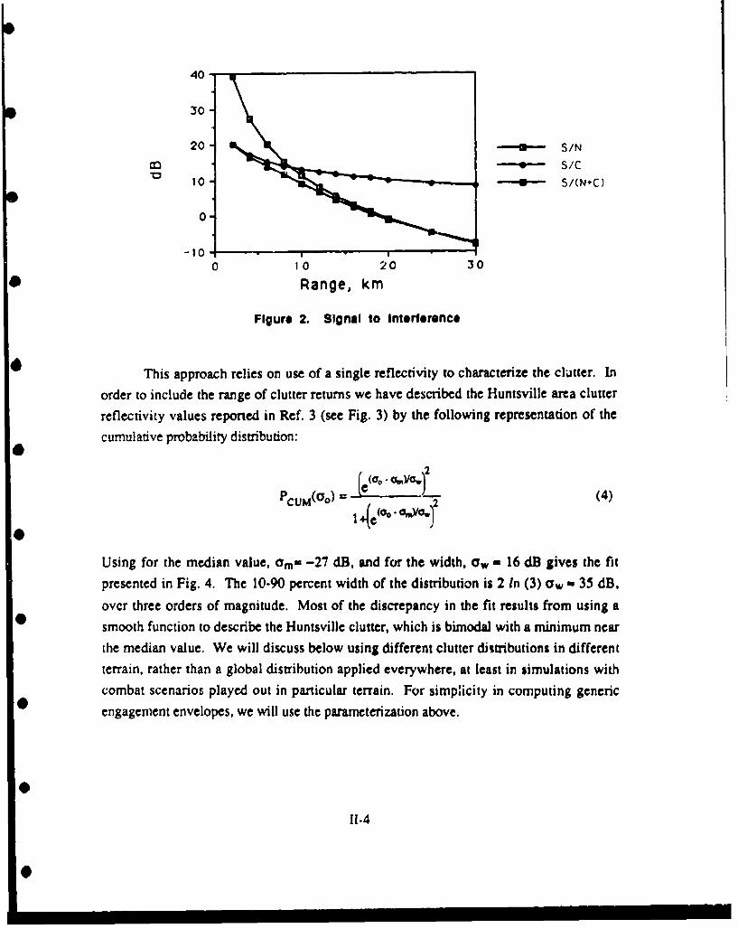
One standard method for incorporating clutter is to compute a signal-to-interference1

(S/I) ratio S/I = S/(N + C), and use S/I in place of S/N to determine PD (R) . We have

assumed a uniform clutter reflectivity such that S/C is 13 dB at 10 km. This example has

been set up so that clutter and noise are comparable at 10 kmi. This is shown in Fig. 2where S/I is dominated by clutter inside 8 km and by noise outside 10 km. Returning to

Fig. 1, we see that computing PD using S/I shortens the engagement envelope by a couple

of kilometers.

I1-3

40-

30

20 - S/N

---O- S/C

"10- 0-- S/(N*C)

0-

-10 -0 10 20 30

Range, km

Figure 2. SIgnal to Intlrterenco

This approach relies on use of a single reflectivity to characterize the clutter. In

order to include the range of clutter returns we have described the Huntsville area clutter

reflectivity values reported in Ref. 3 (see Fig. 3) by the following representation of the

cumulative probability distribution:

2

PCUM(Oo) (00.06Gu)_ (4)

Using for the median value, am- -27 dB, and for the width, ow - 16 dB gives the fit

presented in Fig. 4. The 10-90 percent width of the distribution is 2 In (3) aw - 35 dB,

ovcr three orders of magnitude. Most of the discrepancy in the fit results from using a

smooth function to describe the Huntsville clutter, which is bimodal with a minimum near

the median value. We will discuss below using different clutter distributions in different

terrain, rather than a global distribution applied everywhere, at least in simulations with

combat scenarios played out in particular terrain. For simplicity in computing generic

engagement envelopes, we will use the parameterization above.

11.4

0i

1'LAND CLUTTER

HUNTSVILLE. ALABAMA, AREA,-25-km RADIUS, HORIZONTAL SEAM,L-BAND. a.pseo PULSE,

10 - w 1.3' AZIMUTH, HORIZONTAL POLARIZATION-241 SAMPLES OUT OF 2,000

U I

IO0 • -.

2

8O

ma

2

0

t -60-5 -509 -40 -41 -20 -25 -0 -1 1I0 5 -

Figure 3. Enionmenaio Rada Cluntsler Distributions

100-

Uj 0

20-

-2 60 50 -40 -30-2 29 -2 0 I -10 I , -

Figure 4. Envpaironmna Rada Cutsiluter Distribution!

To compare the approach of Eq. 3 to the S/I approach, we assume the radar

parameters arc such that a threshold based on an S/C requirement of 13 dB leads via Eq. 3to a 50 percent probability of detection at 10 km for the Huntsville p(Oo). if the effects ofnoise are neglected. This is the same as would have been obtained with the signal-to-interference method if noise were neglected there also. However, as we see in Fig. 5, thecurve describing the probability that S/C ? 13 dB = 20 (solid diamonds) is very flatcompared to PD curves, whether S/N or S/I is used (open squares, or any curves from

Fig. 1).

1.0

> 0.82 'D(N *C)

0 -6 - N,- P ( 2 0 C ).j 06 ; PD*P(5>20C,1

0.4000

0CL 0-2-

0.0 , i

o1o 20

Range, km

Figure 5. Clutter-Limited Detection

Neglecting noise altogether is clearly inadequate. We propose as a surrogate for theoverall probability of detection limited by both noise and clutter the product of probabilities:

P,) (R) = PC) (R) 4R(5

which is represented by the solid squares. This curve is very different from the curveobtained by replacing S/N with S/(N + C) (open squares). Inclusion of the full clutterdistribution shows that some protection is provided even at very short ranges. Changingthe width parameter to aw = 6 dB yields a much narrower clutter distribution, but theexpected probability of escaping detection is still significant at short ranges.

Thus far we have been considering a single scan. The scan-to-scan behavior can bercgarded as correlated or uncorrelated depending on whether or not there is motion from

11-6

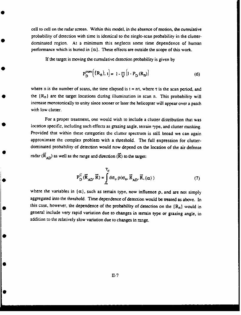
cell to cell on the radar screen. Within this model, in the absence of motion, the cumulative

probability of detection with time is identical to the single-scan probability in the clutter-

dominated region. At a minimum this neglects some time dependence of humanperformance which is buried in ((x). These effects are outside the scope of this work.

If the target is moving the cumulative detection probability is given by

lc (n1 )=I-rl'(l-P(R" (6)

where n is the number of scans, the time elapsed is t = nc, where r is the scan period, andthe (Rn) are the target locations during illumination in scan n. This probability willincrease monotonically to unity since sooner or later the helicopter will appear over a patch

with low clutter.

For a proper treatment, one would wish to include a clutter distribution that waslocation specific, including such effects as grazing angle, terrain type, and clutter masking.

Provided that within these categories the clutter spectrum is still broad we can againapproximate the complex problem with a threshold. The full expression for clutter-dominated probability of detection would now depend on the location of the air defense

radar (RAD) as well as the range and direction (R) to the target:

C f-PD (RAD, R) = dao p(7 0 , RAD, R, {lo}) (7)

where the variables in (a), such as terrain type, now influence p, and are not simply

aggregated into the threshold. Time dependence of detection would be treated as above. Inthis case, however, the dependence of the probability of detection on the (Rn) would in

general include very rapid variation due to changes in terrain type or grazing angle, inaddition to the relatively slow variation due to changes in range.

1-7

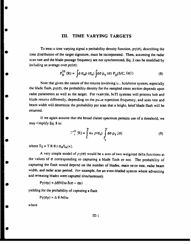
III. TIME VARYING TARGETS

To treat a time varying signal a probability density function, pT(a), describing thetime distribution of the target signature, must be incorporated. Then, assuming the radarscan rate and the blade passage frequency are not synchronized, Eq. 2 can be modified byincluding an average over pTr(a):

* PD (R) = d COP (aC0 ) fda PT (a) PD(S/C, {CE}) (8)

Note that given the nature of the returns involving t,-- hub/rotor system, especiallythe blade flash, pjr(a), the probability density for the sampled cross section depends upon

radar parameters as well as the target. For nxarrple, MTI systems will process hub andblade returns differently, depending on the pu;se rcpetition fr:,uency, and scan rate andbeam width will determine the probability per scan that a bright, brief blade flash will be

returned.

* It we again assume that the broad clutter spectrum permits use of a threshold, we

may cimplify Eq. 8 to:

R)$ ,,- (FOO f da PT 'a) (9)

*£TS

where TS = T R 0 r aO/Isc(v).

A very simple model of j-(a) would be a sum of two weigi~ted delta functions atthe values of ay corresponding to capturing a blade flash or not. The probability of

capturing the flash would depend on the number of blades, main rotor rate, radar beamwidth, and radar scan period. ?cr example, for an even-bladed systvm where advancing

and retreating blades were captured simultaneously

* PT(oF) = AONf/o 8(a - 7F)

yielding for the probability of capturing a flash

PT(OF) = A 0 Nf/a,

where

IH-l1

AO = radar beam width (10)

w = scan rate

N = n'imber of blades

f = rotor frequency, and

PT(oNF) I - PT (aF).

In such a simple case the integral over signature could be replaced with a two-term

sum with different thresholds for the remaining integral over clutter reflectivity. Thiswould give for a single-scan probability of detection for a helicopter over a randomly

selected ground patch

TF N

PD (R) = P (oF) fdao p(ao) + P(aoN') f doo p(oo) (II)

where the upper limits are defined as in Eq. 3.

Generally speaking, if the helicopter is hovering or moving very slowly the timevarying signature dominates the detection. Assuming the helicopter is essentially stationaryover a particular grounc patch with a fixed value of clutter reflectivity, a.,

P; (Rado)= dop(u) (12)

TS

For a given 0(o, a signature distribution with just two values would reduce to eitherunity, PT(aF), or zero for the probability depending on whether both values, only thehigher, or neither resulted in detection. In general, the cumulative probability of detectionwould be given by

P; (R,t, o) I -PD(R, co) (13)

To compute an aggregated cumulative probability this result is averaged over thedistribution of ao values:

cu (R,t)= doo p(oo) PcuD (R, t, oo) (14)

Im-2

We have not included system noise or location specific clutter reflectivity

distributions in this discussion. These features can be included in the same fashion as in

Chapter II.

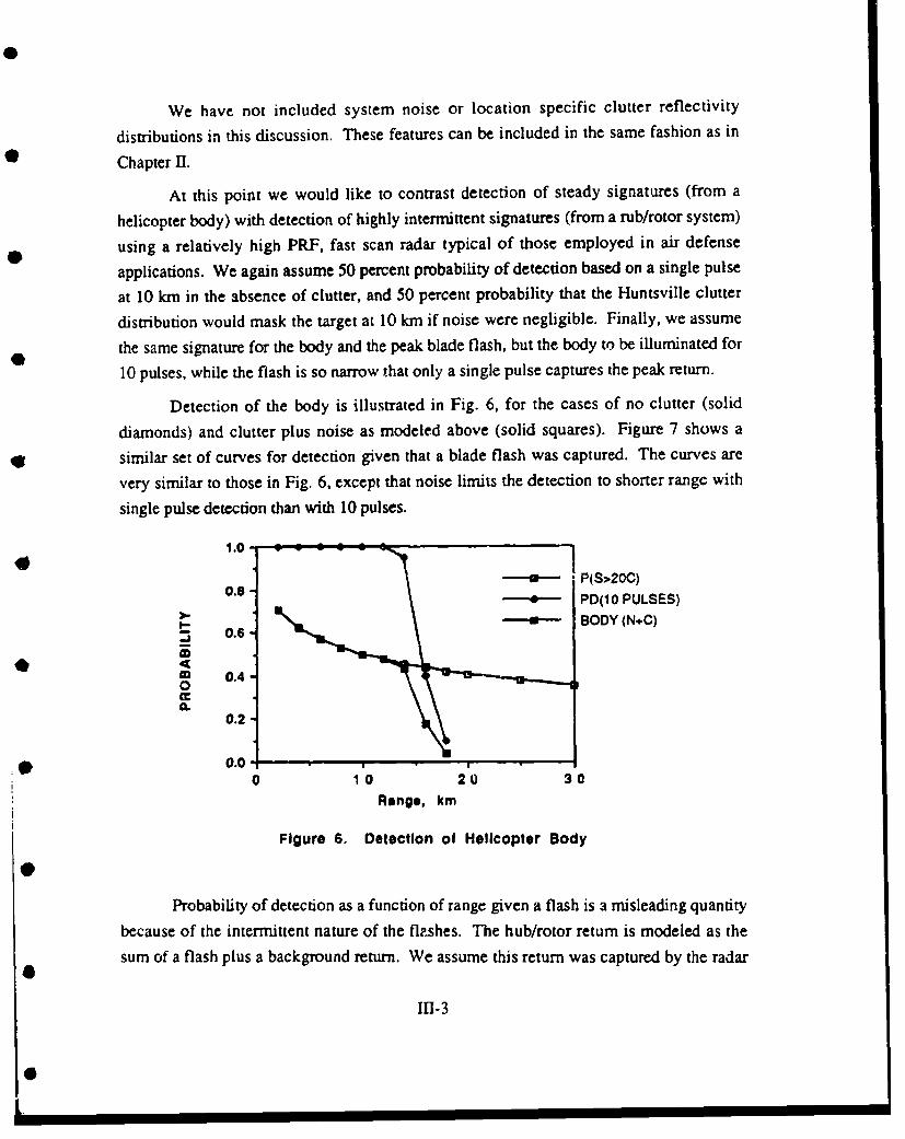
At this point we would like to contrast detection of steady signatures (from a

helicopter body) with detection of highly intermittent signatures (from a rub/rotor system)

using a relatively high PRF, fast scan radar typical of those employed in air defense

applications. We again assume 50 percent probability of detection based on a single pulse

at 10 km in the absence of clutter, and 50 percent probability that the Huntsville clutter

distribution would mask the target at 10 km if noise were negligible. Finally, we assume

the same signature for the body and the peak blade flash, but the body to be illuminated for

10 pulses, while the flash is so narrow that only a single pulse captures the peak return.

Detection of the body is illustrated in Fig. 6, for the cases of no clutter (solid

diamonds) and clutter plus noise as modeled above (solid squares). Figure 7 shows a

*- similar set of curves for detection given that a blade flash was captured. The curves are

very similar to those in Fig. 6, except that noise limits the detection to shorter range with

single pulse detection than with 10 pulses.

1.0- ,

0.8- PiS>20C)0.6 -PD(10 PULSES)

p> BODY (N÷C)

. 0.6

0 0.4

0.2

0.0

0 10 20 30

Range, km

Figure 6. Detection of Helicopter Body

Probability of detection as a function of range given a flash is a misleading quantity

because of the intermittent nature of the flashes. The hub/rotor return is modeled as the

sum of a flash plus a background return. We assume this return was captured by the radar

IM-3

at the flash level for a single pulse 10 percent of the time, and a much lower hub return90 percent of the time. Assuming the hub return to be 10 dB lower leads to a probability ofdetection indicated by the open diamonds for detection by a single pulse off the blade or10 pulses off the hub. For ease of comparison the noise plus clutter limited body and rotordetection probabilities are repeated in Fig. 8 and a case with the hub 20 dB (solid diamond)

below the rotor flash is added.

1.0-

0.8 --- PD(N)-- P(S>20C)

* -- PD*P(S>20C)S0.6

- -- 10%F+H(-10)

0 0.40

0.2

0.0-0 10 20 30

Range, km

Figure 7. Detection of Blade Flash

0.8•

BODY0.6-01- lOF+H(-10)

I1 00/%F+H(-20)

0.49 m

0

I. 0.2

0.00 10 20

Range, km

Figure 8. Comparison of Body versus Rotor Detection

If1-4

IV. IMPROVING THE TREATMENT OF CLUTTER IN

COMBAT MODELS

SSimple engagement envelopes, like those presented in Chapters II and III, are

useful for qualitative comparisons and for demonstrating the importance of features to beincluded in more detailed analysis. These chapters show that the large width of clutterdistributions is a feature which warrants inclusion in models such as JANUS andCASFOREM, at least when they are used to support acquisition decisions involvinghelicopters, other vehicles operating in clutter, or the radar-directed weapons that engagethem. In this chapter we will discuss how to incorporate the effects of clutter in theengagement of helicopters by air defense systems.

A. MASKING

Since use of terrain masking is a primary helicopter survivability tactic, modelsusually do not permit engagement when the helicopter is masked. This approach should beextended to set the clutter return to zero if the ground in the same range gate with the targetis masked. We believe that this would be a relatively simple coding change since the line-of-sight algorithm used to determine visibility of the helicopter could also be used todetermine visibility of the ground. This change would increase the detectability of targetsuniformly. It is difficult, however, to assess in the abstract how important this change willbe, because it is likely to h. very dependent on terrain and on mission. Nevertheless,implementation should be so simple that we believe this is the number one improvement tobe made in modeling effects of clutter for those codes where masking of ground clutter isnot already incorporated.

B. USE OF A UNIVERSAL CLUTTER DISTRIBUTION

Clutter reflectivity distributions depend on the radar's frequency, polarization andresolution cell size, as well as environmental features such as terrain type, grazing angle,man-made featurcs, and vegetation cover. By a "universal" distribution %,.- mean oneapplied to the entire globe, but which at least acknowledges the well-known dependence of

0 clutter reflectivity on radar frequency. To sample the clutter distribution would require

'V-I

S

some sort of random draw, but several conditions must be applied if this random draw is to

make both physical and operational sense.

First, the distribution must be based on map coordinates in a way that is

reproducible if vehicles leave and return to a specific location. Additionally, it would be

desirable for correlations to exist among the clutter refiectivities computed at various ranges

along the same azimuth from the target.

Second, as the location of the illuminated ground patch changes, the clutterreflectivity should not change much over a region small compared to a beam illumination

region.

Finally, as the azimuth from the illuminated ground ratch changes, the clutter

reflectivity should change smoothly. We are uncertain at present of the phenomenology

necessary to quantify this statement further.

There are two basic ways to implement such a scheme. The first approach woulduse extra fields in the map data to record clutter reflectivities with azimuthal, frequency andgrazing angle dependence. If these numbers were measured for a given location so muchthe better. If not measured, they could be estimated, consistent with knownphenomenology. The second approach would be to choose co values corresponding torandomly generated values of the cumulative probability satisfying the above listedrequirements. More importatt, probably, would be to proceed with families of clutterdistributions characteristic of specific locales, as discussed below.

C. USE OF LOCAL CLUTTER DISTRIBUTIONS

Clutter reflectivity distributions depend on the fre-quency, polarization, and spatialresolution of the radar, as well as environmental features such as tcrrain type, grazingangle, man-made features and vegetation cover. In order to obtain a single graph thatindicates the characteristic vulnerability of a particular helicopter type to at given air defensesystem aggregating all the environmental features to obtain a single distribution for thepurposes of analysis is acceptable. In the context of a detai.ed war game used forsupporting acquisition decisions or training commanders, however, our full knowledge ofthe phenomenology should be incorporated.

There is still a shortage of data for ground-based radars. The following generaiconsiderations seem likely to apply, and can be used to outline future work. First, thebroad distributions observed in nature (Fig. 3) are likely to be made up ol several

IV-2

II

distributions, for different terrain types, with different medians. These "fundamental"

distributions are probably much less broad individually than is their sum. Finally, the

median value (and possibly also the width) for a given terrain type will depend on the

grazing angle between the radar transmitter and the illuminated ground patch. Given the

knowledge of how the global distributions break down by terrain type, etc., the procedures

outlined in Section IV.B could be extended.

For map-based war games using Defense Mapping Agency (DMA) data bases the

needed information on terrain and grazing angle is available. To the extent that these

features matter, they should be incorporated correctly in operational effectiveness studies

and ,-arin'g exercises. A much more ambitious program would be to use these

co:isideratioins in mission planning and execution (Ref. 4).

D. SUMMARY

The most important improvement in clutter modeling is also the easiest to implement

in current models: If the terrain is masked set the clutter to zero.

To incorporate the broad range of clutter reflectivity, values using a single global

distribution is the simplest next step. A better approach would be to incorporate what is

* known of the phenomenology of clutter reflectivity. Low-flying aircraft exploiting terrain

will not find themselves exposed over random patches of terrain. Neglecting posible

correlations between exposure points and clutter values could be very misleading in war

games used for training or for ana'ysis.

IV-3

SD

V. EXPECTED IMPACT ON STUDIES

In this chapter, we will anticipate the effects the model improvements outlined

earlier are likely to have.

Terrain-specific combat models must include line of sight to both targets and clutter.

To our knowledge, line of sight to targets is generally treated, but some models assume

clutter returns are always present, even if the ground is masked. Modeling techniques that

account for masking of clutter will show enhanced effectiveness of air defense radars and

reduced effectiveness of low-flying aircraft. Radars with such high clutter suppression or

helicopters with such large signature that clutter never affords protection will be exceptionsto this rule. An important question is "how often will helicopters be exposed while theground under them is masked?" This can only be addressed in the context of exercise or

war games focusing on specific missions and terrain.

Including the width of clutter distributions in the engagement of transiting targetsleads to a probability of detection that limits very slowly to unity at short ranges. The

timelines for engagement at short ranges will increase, but the possibility of engagement at

long ranges may 1e. lightly increased. Clutter will afford protection some of the time, even

at very short range. This is a common experience in the field, but is often not reflected in

combat models.

Modeling of hovering helicopters is still at a rudimentary level. We believe that theprimary impact of the approach outlined here will be to change the modeled timelines for

engagement. The changes are difficult to predict. It is likely that the distribution of

timelines will be very broad, and cannot be modeled with a single delay.

V-I

REFERENCES

D.A. Sparrow, 1. Kay, R.R. Legault, J. Ralston, and W. Shafter, Active and PassiveAids to Survivability for LHX (U), Institute for Defense Analyses, IDA PaperP-2285, January 1990 (SECRET/NOFORN/WNINTEL).

2. Merrill I. Skolnik, Radar Handbook, McGraw-Hill, 1970.

3. Fred E. Nathanson, Radar Design Principles, McGraw-Hill, 1969.

4. This possibility was brought to our attention by Maj. Gary Davis (USA).

R-1

APPENDIX

TIMELINES AND M-OUT-OF-N RULES

A-1

I.

6

APPENDIX

TIMELINES AND M-OUT-OF-N RULES

Rules that impose constraints on whether or not to declare a detection based on a

sequence of events are common in signal processing, both human and electronic. The

earliest use of an m-out-of-n rule of which we are aware was descriptive: During World

War II radar operators did not generally declare a target with a single scan, but waited for

confirmation on one of the next two scans. This behavior was described as following a

2-out-of-3 rule for detections--a blip was required two times in three scans.

Beyond modeling human behavior such constraints are often imposed

electronically, for example through requiring 20-out-of-30 pulses per scan, or 2-out-of-4

available doppler bins before a declaration is made. Electronic tests operating on a single

scan affect the single scan probability of detection. The cumulative probabilities are

straightforward to calculate from the underlying probabilities.

On the other hand, m-out-of-n rules applied to sequential scans alter the cumulativeprobability timelines in ways that can be difficult to calculate. In this appendix we outline

the general algorithm, in the form of a recursion relationship, for computing how detectionprobability accumulates under an m-out-of-n rule. This solution is illustrated for the case of

2-out-of-3. A general solution is presented for the case of m-in-a-row. Cumulative

probability and individual probability versus number of scans are computed for severalvalues of PD for the 2-out-of-3 rule. Several cases of how Cumulative probabilities depend

on range through the decrease of the single-scan probabilities with range are also presented.

A. GENERAL SOLUTION

A straightforward description of an algorithm to compute the m-out-of-nprobabilities follows. First, one defines a vector with elements given by the probabilities

*- that after j steps the m-out-of-n rulc has not been satisfied, and the final n - I elements in

the string of hits and misses is specified by the set (a). One final element is the

probability that a detection has occurred at or before this step:

Vj .. I {PND( a),J)), PD)]

A-2

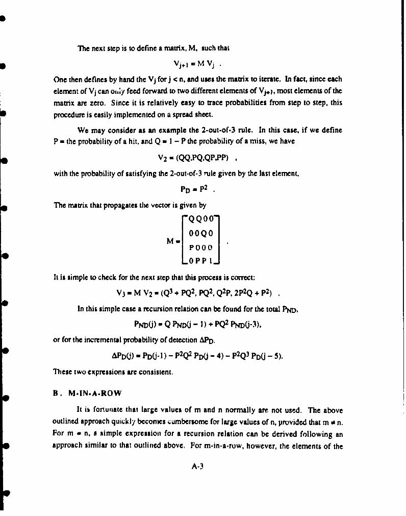
The next step is to define a matrix, M. such that

Vj+1 = M Vj .

One then defines by hand the Vj for j < n, and uses the matrix to iterate. In fact, since each

element of Vj can oi;y feed forward to two different elements of Vj+1, most elements of the

matrix are zero. Since it is relatively easy to trace probabilities from step to step, this

procedure is easily implemented on a spread sheet.

We may consider as an example the 2-out-of-3 rule. In this case, if we define

P - the probability of a hit, and Q - I - P the probability of a miss, we have

V2 - (QQPQ,QPPP) ,

with the probability of satisfying the 2-out-of-3 rule given by the last element,

PD-p 2

The matrix that propagates the vector is given by

-QQOO0

00Q0M=MPO00

_PP 1_

It is simple to check for the next step that this process is correct:

V3 - M V2 - (Q3 + pQ2 . pQ2 , Q2p, 2p 2Q + p2)

In this simple case a recursion relation can be found for the total PND,

P ND) - Q NDO - ) + pQ2PNDO-3),

or for the incremental probability of detection ArPD.

APDO) - PD(,j-I) - p2Q2 PDOj - 4) - p2Q3 PD(J - 5).

These two expressions are consistent.

B. M.IN.A.ROW

It ib fortunate that large values of m and n normally are, not used. The above

outlined approach quickly becomes ,;umbersome for large values of n, provided that m * n.

For m - n, 0 simple expression for a recursion relation can be derived following an

approach similar to that outlined above. For m-in-a-row, however, the elements of the

A-3

vector are strings which have never had m-in-a-row hits, the first element ending in a miss,

then a miss followed by a single hit. a miss followed by 2 hits..., a miss followed by m -

1 hits, and finally a string which has satisfied m-in-a-row at some time in its history:

V(PND(...0), PND(...01), PND(...011),...PD).

This results in the general expression for m-in-a-row

PNDQ•() = I 0!5;j < m

PND(J) -QI - DO2:

i-l

This can be checked by evaluated PND for the first non-tivial case, j = m, which

gives:M

PDOJ) = Q X pi-1i-I

IQll-.P m _=

I1-P r

Finally, we note that the PND(j) exhibit an exponential behavior for large j. In other

words, in the limit as j becomes infinite PND(j + 1)/PN(j) becomes a constant. This is

trivially correct for m = 1, and appears to be true for all m and n. However, we have notfound a way to exploit this to simplify analyses.

C. SAMPLE CALCULATIONS USING A 2-OUT-OF-3 RULE

In general for m-out-of-(2m - 1) detection rules a single-scan probability of

50 percent accumulates to 50 percent after (2m - 1) scans. Hence, for single-scan

probabilities greater than 50 percent, cumulative probabilities tend toward unity very fast.

In Fig. A-I we show how probabilities accumulate for low single-scan PD. For moderate

scan numbers, the cumulative probability is most sensitive to changes in the single-scan

probability in the 0.1 to 0.2 range.

The probability per scan is plotted in Fig. A-2 for three values of PD. We note firstthat for aircraft attrition rates of a few percent are generally considered unacceptably high.

Even low per scan probabilities satisfy the 2-out-of-3 rule on the second or third scans at

rates of a few percent. The cumulative probability derived from a 2-out-of-3 rule always

peaks on either the second or third scan, depending on whether the single-scan probability

is greater or less than 50 percent.

A-4

1.0 - I,

0.6 owe PCUM(.1)-.-- PCUM(.3)

73 0., - PCUM(.")F O PCUM(.2)

Im 0.4 -

0.02

0 10 20 30 40

SCAN NUMBER

Figure A-1. Cumulative Probability for 2/3 Rule

0.15'

- -P=0.1

-9-P.0.2

-"-- P.0.3S0.105

0 o.0o.

0.•IL 0.001

_ -- -0 10 20 30

SCAN NUMBER

Figure A-2. Probability per Scan

We wish to examine what happens with these cumulative probabilities when viewedas a function of range for a fixed scan number rather than as a function of scan number fora fixed single-scan PD. We use the new model for noise and clutter together, requiringboth that S/C be greater than 13 dB, and that S/N lead to detection. This proceduregenerates the single-scan probability of detection indicated by the solid squares in Fig. A-3,and is repeated in Fig. A-4 here as open circles. At each range, this single-scan probabilityis used to generate a cumulative probability after 3, 5, and 10 scans. We see as expectedthat the probability accumulates fairly fast if the single-scan P3 is above 0.5. In otherwords, as the number of scans increase the cumulative probability curve gets steeper at theedge.

A-5

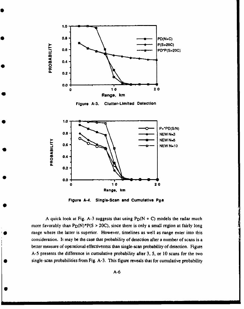
1.0-

0.8 - PD(N+C)

>_.- P(S-20C)

"0.6 PD'P(S>20C)

* 0.40

0.2

0.00 10 20

Range, km

Figure A-3. Clutter-Limited Detection

*1.0- a

-- 0- P>*PD(SN)0.8-- NEW NU3

-U- NEW N=60.6-. NEW N=5I--

0 0.40CO.

0.2

0 10 20

Range, km

Figure A-4. Single-Scan and Cumulative PD$

A quick look at Fig. A-3 suggests that using PD(N + C) models the radar much

more favorably than PD(N)*P(S > 20C), since there is only a small region at fairly long

range where the latter is superior. However, timelines as well as range enter into this

consideration. It may be the case that probability of detection after a number of scans is a

better measure of operational effectiveness than single-scan probability of detection. Figure

A-5 presents the difference in cumulative probability after 3, 5, or 10 scans for the two

single-scan probabilities from Fig. A-3. This figure reveals that for cumulative probability

A-6

0 . .

after many scans, performance that is slightly better in the low single-scan PD regime is

more important than performance much better in the high PD regime.

O delta PD N,-3

" \ delta PD N-5

-S--della PD N-10p 5

0 0.0

0.

I--

0

.0.4

0 1 20

Range, km

Figure A-S. Delta PD Versus Range for Three Scan Numbers

Finally, we compare how the same fundamental probabilities accumulate for

moving and stationary targets: the key difference is that the clutter does not change under a

stationary helicopter.* In other words, the probability that S > 20C cannot be allowed to

accumulate to unity, since the clutter is whatever it is near the h.-icopter. In Fig. A-6, a

given single-scan probability based on a product of noise and clutter probabilities is

accumulated. For the solid diamonds, the entire probability is used, corresponding to

significant scan-to-scan variation in the background clutter. For the solid squares, only the

probability that noise limits detection is allowed to decay away, corresponding to a target in

a fixed clutter cell. The differences are striking in the region where clutter dominates the

single-scan PD.

The formal assumpuon that the fundamental scan-to-scan probabilities is the same is critical here;clearly hovering and transmiiUng helicoptrs have very different singlc-scan detection probabilities inmost cases.

A-7

1.0 :1.0

P>'PD(S/N)

0.8 .- MOVING N-10-0--- STATIONARY Na1 0

S0.6

o 0.40aC

0.2

0.010 5 10 15

Range, km

Figure A-6. Cumulative Probabilities for Two Cases

A-8

L