Modeling of the very low pressure helium flow in the

LHC Cryogenic Distribution Line after a quench

Benjamin Bradua,b,, Philippe Gayeta,, Silviu-Iulian Niculescub,, EmmanuelWitrantc,

aCERN, CH-1211 Geneve 23, SwitzerlandbLaboratoire des Signaux et Systemes, UMR CNRS 8506, CNRS-Supelec, 3 rue Joliot

Curie, 91192, Gif-sur-Yvette, FrancecGipsa-lab,University Joseph Fourier, B.P. 46, 38 402, ST. Martin d’Heres, France

Abstract

This paper presents a dynamic model of the helium flow in the Cryogenic

Distribution Line (QRL) used in the Large Hadron Collider (LHC) at CERN.

The study is focused on the return pumping line, which transports gaseous

helium at low pressure and temperature (1.6 kPa / 3 K) over 3.3 km. Our

aim is to propose a new real-time model of the QRL while taking into ac-

count the non-homogeneous transport phenomena. The flow model is based

on 1D Euler equations and considers convection heat transfers, hydrostatic

pressure and friction pressure drops. These equations are discretized using

a finite difference method based on an upwind scheme. A specific model

for the interconnection cells is also proposed. The corresponding simulation

results are compared with experimental measurements of a heat wave along

the line that results from a quench of a superconducting magnet. Different

hypotheses are presented and the influence of specific parameters is discussed.

Key words: Helium (B), Heat transfer (C), Fluid Dynamics (C),

Email addresses: benjamin.bradu@cern.ch (Benjamin Bradu)

Preprint submitted to Cryogenics October 30, 2009

Numerical Simulation (F), Transmission lines (F)

1. Introduction

In 2008, the European Organization for Nuclear Research (CERN) started

the most powerful particle accelerator of the world, the Large Hadron Collider

(LHC). The LHC accelerates proton beams which are driven by supercon-

ducting magnets maintained at 1.9 K over a 27 km ring. To cool-down and

maintain superconductivity in different magnets, large helium refrigeration

plants are used [1].

The LHC cryogenic systems are divided into 8 equivalent cryoplants

around the LHC ring and each of them supply helium to superconduct-

ing magnets over 3.3 km via a Cryogenic Distribution Line (called QRL)

installed underground in parallel to magnets [2]. The dynamic behavior of

helium flows in the QRL is not well understood, especially during transients

as after a quench. To the best of the authors knowledge, relevant dynamic

models for such a cryogenic line do not exist, due to the system specifici-

ties (length, interconnections, gaseous helium at cryogenic temperature and

at low pressure). Thus, this paper provides a numerical dynamic model for

gaseous helium flows in long cryogenic lines that contain interconnections

with heat transfers.

Previously, a real-time dynamic simulator for cryogenic systems called

PROCOS and using the modeling software EcosimPro c© was developed at

CERN [3]. In this context, the model of a 1.8 K refrigeration unit for the

LHC achieved to simulate the pumping over the QRL performed by the cold-

compressors [4].

2

The model of the QRL flow is embedded in a larger model that aims

at operator training, diagnostic and control improvements. Thus, the QRL

model must be computed fast enough to obtain simulations faster than real-

time in case of operator training.

First, the paper presents briefly the cryogenic distribution line of the

LHC and its interconnections to the main cooling loops. Then, the numerical

model of the return pumping line at very low pressure is detailed: the model

of the flow, the heat transfers and the pressure drops are described with their

numerical implementations in Section 3. Next, steady-state and dynamic

simulations during a quench are presented in Section 4. The presented results

are discussed and compared with real data obtained in 2008.

2. The Cryogenic Distribution Line

The QRL is composed of five different headers (called B, C, D, E, F)

with temperatures ranging between 4 K and 75 K to supply magnets, beam

screens and thermal shields of the magnet cryostats, see Figure 2. All main

QRL elements as inner headers and internal fixed points are built in stainless

steel AISI 304 L.

A LHC sector of 3.3 km is divided into different cryogenic cells that

constitute the elementary cooling loops. A sector is composed of 23 standard

cells of 106, 9 m (composed of 6 dipoles and 2 quadripoles) plus other specific

cells according to the sector considered, see Figure 1 where the sector 5-6 of

the LHC is represented. The main cooling loops are supplied in supercritical

helium by the header C and the helium flows are returned back to the header

B through sub-cooled heat exchangers.

3

Q1/Q2/Q3

QRL - Header C

Q4/D2/Q5/Q6/

DFBQ7/Q8 Q9/

Q10

DS 5R = 184m

P5

CMS

D1 D2 D3 Q1 Q2D1 D2 D3

1standard cell = 106.9m

ARC : 23 cells

LSS 5R =269m ARC = 2459m

Q11 Q8/Q9/Q10

Jumper/DFB/Q5Q4

LSS 6L=269mDS 6L=170m

P6

QUI

S9701.8 K

Sector 5-6 = 3351 m

EH970Supercritical helium : 3 bar / 4.6 K

Gaseous helium , Very Low Pressure : 16 mbar / 4 K

DS = Dispersion SuppressorLSS = Long Straight Section

RM = Return moduleQUI = Cryogenic interconnection box

RM

D : Dipole magnetQ : Quadripole magnet

DFB : Distribution Feed Box

1.8 K refrigeration unit4.5 K

Refrigerator

3.5K8g/s

Cold compressorsWarm compressors

3.5K0.8g/s

3.5K0.8g/s

3.5K0.8g/s

3.5K0.8g/s

3.5K1.3g/s

3.5K3.8g/s

3.5K0.7g/s

3.5K2.4g/s

QRL - Header B

Figure 1: Details of the LHC sector 5-6 with the main cooling loops for the superconducting

magnets

3. Modeling of the header B

Helium is considered as a perfect fluid : viscosity and thermal conduc-

tivity are neglected as helium has a very low viscosity (µ ≈ 10−6 Pa.s) and

a very low thermal conductivity (λ ≈ 10−3 W.m−1.K−1). Moreover, gaseous

helium is considered as a compressible gas.

3.1. Modeling of the Flow

First, the main flow line is modeled, neglecting interconnections. Accord-

ing to previous assumptions, an inviscid flow in the header B is considered.

Thus, the flow can be described by Euler equation which is obtained from

Navier-Stokes equation neglecting the viscosity and the thermal conductivity

4

D=104 mm4,6 K, 3 bar

D=154 mm20 K, 1.3 bar

D=84 mm75 K, 18 bar

D=273 mm4 K, 0.016 bar

D=84 mm50 K, 19 bar

Figure 2: QRL cross-section with remarkable data

[5]. The conservative form of Euler equations is the following:

∂

∂t

ρ

~M

E

+ ~∇ ·

ρ · ~V

ρ · ~V T ⊗ ~V + P · I

ρ · ~V ·(u+ P

ρ

) =

0

0

q

(1)

where the different variables are described in Table 1. These three equa-

tions represent mass, momentum and energy balances. The momentum

is defined as ~M = ρ · ~V and the total energy per unit volume is E =

ρ ·(u+ 1

2· (V 2

x + V 2y + V 2

z )).

The following assumptions on the flow are assumed :

• flux according to the x direction only (the main flow direction) : V = Vx

and M = ρ · Vx;

• straight line. The QRL curvature (radius of curvature of 4.3 km) has

a negligible impact on the flow;

• in operational conditions, the kinetic component can be neglected: ρ ·

|~V |2 << P , which implies that ρ · ~V T ⊗ ~V + P · I ≈ P · I.

5

Considering the above approximations, Euler equation (1) can be ex-

pressed in 1D as:

∂X(x, t)

∂t+ F (X) · ∂X(x, t)

∂x= Q(x, t) (2)

where X = [ ρ M E ]T is the state vector, F is the Jacobian flux matrix

and Q = [ 0 0 q ]T is the source vector.

3.1.1. Modeling for an ideal gas flow

To compute the Jacobian flux matrix, it is necessary to include an equa-

tion of state to link pressure, density and internal energy. First, an ideal gas

is considered: it is assumed that u = Cv · T , which leads to the following

equation of state:

P = ρ ·R · T = ρ · u · RCv

= ρ · u · γ (3)

where the constant γ = (γ − 1). For this case, the Jacobian matrix was

calculated in [5, 6] as:

F =

0 1 0

(γ−3)V 2

2(3− γ)V γ

γV 3 − γV Eρ

γEρ− 3γV 2

2γV

(4)

and the eigenvalues of the Jacobian are:λ1 = V + c

λ2 = V

λ3 = V − c

(5)

6

where c is the speed of sound, defined by:

c =√γRT =

√γP

ρ=

√γγ(

E

ρ− V 2

2) (6)

All the eigenvalues of the Jacobian are real and distinct. This means that

Eq. (2) is a strictly hyperbolic system of equations. Moreover, for subsonic

flows (V < c) there are two positive eigenvalues and one negative eigenvalue:

informations are propagated forward and backward and the eigenvalues rep-

resent the different speeds of propagation.

3.1.2. Modeling for a gaseous helium flow

The previous equations cannot be directly applied to helium flows at low

temperature as the equation of state (3) is not valid anymore. Hence, the

following empirical formulation for the helium internal energy is considered:

u = u0 + Cv · T (7)

where u0 = 14950J.kg−1 is a constant. This equation remains valid for

gaseous helium at low pressure (P < 10 kPa), with a relative error less than

1 % between 1.8 K and 300 K. For higher pressures, this equation is still

valid for gaseous helium far from the saturation line and far from the critical

point.

We are interested in simulating the helium flow during the final cool-

down of magnets from 4.5 K to 1.8 K. During this phase, the pressure

in the header B decreases from 0.1 MPa to 1.6 kPa and temperatures are

between 2 K and 10 K. Within these ranges, Eq. (7) remains valid and the

equation of state and the sound velocity for helium become respectively:

7

P = ρ ·RHe · T = ρ · (u− u0) · γ (8)

c =

√γγ

(E

ρ− V 2

2− u0

)(9)

A new Jacobian flux matrix is computed with additional terms containing

the constant u0 :

F =

0 1 0

(γ−3)V 2

2− u0γ (3− γ)V γ

γV 3 − γV Eρ

γEρ− γ(3V 2

2+ u0) γV

(10)

and the eigenvalues are the same as for an ideal gas, see Eq. (5). Thus,

the system of equations is still a strictly hyperbolic system with the same

propagation speeds than for ideal gases but the dynamics is different.

3.2. Discretization Scheme

To solve numerically the system of partial differential equations, the flow

is discretized in N nodes, see Figure 3. A finite difference method was chosen

to compute space and time derivatives using a first order upwind scheme, as

suggested in [6]. The time discretization is performed according to an implicit

discretization scheme based on a backward Euler method. As the cryogenic

line is pumped by cold-compressors, natural Dirichlet boundary conditions

are set as follows:

• the input energy E(0, t) = E1(t);

• the input density ρ(0, t) = ρ1(t);

8

• the output momentum M(L, t) = MN(t).

Hence, mass and energy are propagated forward whereas momentum is

propagated backward, which is in agreement with the signs of eigenvalues ob-

tained in Eq. (5) and with the physics of the flow. As the cold-compressors

are ’pulling’ helium atoms in the line, the momentum propagation is back-

ward whereas the mass (helium atoms) and energy (heat) are naturally trans-

ported with the flow. Thus, in the framework of the upwind scheme, ∂ρ/∂x

and ∂E/∂x are approximated by a first-order backward finite difference and

∂M/∂x is approximated by a first-order forward finite difference. The fol-

lowing algebraic system is then obtained:

Xi(t) +Ai(Xi)

∆xXi(t) +

Bi(Xi)

∆xXi−1(t) (11)

+Ci(Xi)

∆xXi+1(t) = Qi(t)

where i denotes the value at xi and:

Xi =

ρi

Mi

Ei

Ai =

0 1 0

− (γ−3)V 2i

2+ u0γ −(3− γ)Vi −γ

γV 3i −

γViEi

ρi

γEi

ρi− γ(

3V 2i

2+ u0) γVi

Bi =

0 −1 0

0 0 0

−γV 3i + γViEi

ρi−γE

ρi+ γ(

3V 2i

2+ u0) γVi

9

Ci =

0 0 0

(γ−3)V 2i

2− u0γ (3− γ)Vi γ

0 0 0

Qi =

0

0

qi

Ei-1,ri-1 Ei+1,ri+1Ei,riMiMi-1Mi-2 Mi+1 ...

Dx

...

Figure 3: Discretization of the QRL main flow

3.3. Modeling of interconnections

Additional helium fluxes coming from LHC magnets enter in the header

B every 106.9 m in standard cells as depicted in Figure 1. These additional

fluxes are perpendicular to the main flux but their contribution to the mo-

mentum is considered as additive, since it is small compared to the total

flow.

Interconnections are included in the discretization scheme at regular inter-

vals every Nsub nodes. Thus, for Ninter interconnections, the line is discretized

in Nsub ·Ninter nodes, see Figure 4.

The source term Qi of interconnection nodes is now augmented to include

the incoming mass, momentum and energy, and consequently writes as:

10

i=(j-1)*Nsub+1

6 7 8 9 10

Mext1

Eext1

Dx

11 141312 151 432 5

Mext6

Eext6

Mext11

Eext11

M16M0

Figure 4: Discretization of the QRL with interconnections for Ninter = 3 and Nsub = 5

Qi =

Mext

i

∆x

(3− γ)V exti

Mexti

∆x

qi +γEext

i Mexti

ρexti ·∆x − (γ − 1)(

3V ext2i

2+ u0)

Mexti

∆x

(12)

for i = (j−1)·Nsub+1 with j = 1 . . . Ninter. Superscripts ext refer to external

inputs, namely the input fluxes at interconnections. As LHC magnet cooling

circuits are not simulated, the input fluxes variables are the boundary condi-

tions, determined from mass-flow, pressure and temperature measurements

on the real plant.

3.4. Heat transfers

The term qi in the energy balance represents heat transfers between the

fluid and its environments per unit volume in a node. The QRL is well

insulated inside a vacuum jacket using a Multi Layer Insulation (MLI) and

thermal shields to minimise radiation and conduction losses.

Heat losses can be divided in two parts: static losses qstati due to radiation,

conduction and vacuum barriers and dynamic losses qconvi due to convection

between the stainless steel pipe and the fluid:

qi = qstati + qconvi(t, ρi,Mi, Ei) (13)

11

In a former CERN study, the static heat losses were evaluated at 1.92 W/m3

in the header B, this corresponds to 0.1 W/m along the line [7].

To compute dynamically the convection heat transfer between the pipe

and the fluid, supplementary variables are introduced to characterize the

pipe properties: its temperature Tw, its specific heat Cpw, its mass Mw and

its internal surface Sw. The headers are built in stainless steel 304L and the

specific heat can be computed from an empirical logarithmic polynomial of

the 8th order valid between 2 K and 300 K [8]. The convective heat transfer

coefficient hc is computed by:

hci =Nui · kiD

(14)

where the Nusselt number Nu is computed from the Colburn formulation

[9]:

Nui = 0.023 · Pr1/3i ·Re0.8

i (15)

because the flow regime in the header B of the QRL is always turbulent

(Reynolds number Re > 105). Finally the convection heat transfer per unit

volume is computed by the Newton law:

qconvi =hci · Swi · (Twi − Ti)

S ·∆x=

Mwi

S ·∆x· Cpwi ·

dTwidt

(16)

3.5. Pressure drops

The QRL is not perfectly horizontal, the slope varies between −1.5 %

and +1.5 % along the LHC ring, and it results a hydrostatic pressure. This

hydrostatic pressure is not taken into account in previous equations and

should be considered.

12

Moreover, friction phenomena are not embedded (the flow is considered

inviscid) whereas frictions can lead to pressure drops not negligible in the

case of a very low pressure flow as in the QRL. Thus, we propose to replace

the momentum partial differential equation (∂M/∂t + ∂P/∂x = 0) by an

algebraic equation to compute the mass flow mi in each cell (compartmental

approach).

The pressure in a cell is computed using the equation of state (8) and the

total pressure drop in a cell can be computed as the sum of the hydrostatic

pressure difference and the friction pressure drop :

∆Pi = Pi − Pi+1 = ρi · g · dzi + fri ·∆x

D· m2

i

2 · ρi · S2(17)

where dzi is the elevation over the cell i and fri is the Darcy-Weisbach friction

factor. The line B of the QRL can be considered as a smooth pipe and the

flow is always turbulent with a Reynolds number Re > 2 · 104. In this case,

the friction factor can be computed from the empirical formulation of Kakac,

Shah and Aung [12] :

fri = 0.184 ·Re−0.2i = 0.184 ·

(D · mi

S · µi

)−0.2

(18)

Combining (17) and (18) the mass flow is calculated as function of the total

pressure drop:

mi =

((Pi − Pi+1)− ρi · g · dzi

0.184 · ( DS·µi

)−0.2 · ∆x2·D·ρi·S2

)1/1.8

(19)

Finally, the momentum is simply deduced from mi adding the interconnection

momentum :

Mi =mi

S+M ext

i (20)

13

3.6. Numerical implementation

The modeling and simulations are performed on a commercial software

called EcosimPro c©, which is able to simulate systems of differential and alge-

braic equations (DAEs) [10]. Ecosimpro c© uses a DASSL algorithm to solve

the DAE system [11]. This method is based on an implicit time discretization

scheme:

y(t) =yn − yn−1

tn − tn−1

(21)

The non-linear system dynamics is then solved by iterations for time tn us-

ing an implicit Newton-Raphson method. The iteration matrix required by

Newton-Raphsons method calculates a Jacobian matrix numerically using

finite differences. Note that the use of an implicit scheme renders the time

integration robust with respect to numerical errors but its main drawback is

the associated lack of precision.

4. Results and discussion

4.1. Simulation in steady-state

The first task consists in checking that the steady-state reached by the

model under constant boundary conditions agrees with the measured values

on the QRL. The header B is equipped with temperature sensors every 200 m

but there is only one pressure sensor and one mass-flow sensor at the end

of the header. Each interconnection also has a virtual flow meter allowing

to estimate the mass-flow in each cell and the electrical heater power in the

phase separator S970 allows us to estimate the mass-flow at the entrance of

the header B.

14

Each of the 8 LHC sectors have the same configuration but they present

some differences at their boundaries. A lot of experimental data were col-

lected in one of these sectors during the hardware commissioning in 2008,

namely sector 5-6 (chosen for this study). Constant boundary conditions

were set in the model, in agreement with the values measured in the sector

5-6 during April and May 2008, when the sector was cold in steady-state.

Pressure and temperature at the entrance were set respectively at 1.630 kPa

and 1.8 K, the output mass-flow was set to 58 g/s and the different external

input fluxes are listed in the Table 2.

Static heat losses were evaluated theoretically at 1.92 W/m3 on the header

B but after measurements on the real line, those losses were reevaluated at

1.1 W/m3, which represent a loss of 0.07 W/m along the line.

Figure 5 shows the simulated temperatures, pressures and mass-flows

along the line obtained in steady-state (curves) in comparison with sensor

values (crosses). The simulated temperatures agree with the observed ones

except for the temperature located at 700 m, due to a poor sensor calibration

or to a bad approximation of the first external fluxes. The pressure drop

calculated including the hydrostatic pressure and friction pressure drops gives

a total pressure drop of 110 Pa over the 3.3 km. This pressure drop is pretty

low in the case of the sector 5-6 because it has a negative slope of −1.54 %

and hydrostatic pressure compensates friction pressure drops.

4.2. Dynamic simulation during a quench

When a quench occurs in a superconducting magnet, the resistive tran-

sition releases a huge amount of energy. A quench protection system was

designed to discharge this energy in large electrical resistances in case of a

15

0 500 1000 1500 2000 2500 3000 35001.8

2

2.2

2.4

2.6

2.8

3

3.2

distance(m)

T(K

)

Temperature

0 1000 2000 3000 40001500

1520

1540

1560

1580

1600

1620

1640

distance(m)

P(P

a)

Pressure

SimulationMeasures

0 1000 2000 3000 400025

30

35

40

45

50

55

60

65

distance(m)

m(g

/s)

Mass flow

SimulationMeasures

SimulationMeasures

Figure 5: Temperatures, pressures and mass-flows along the header B in steady-state

compared with experimental measurements

quench, but an important heat flux is briefly induced in the headers B and

D of the QRL (the return lines), thus creating a propagated heat wave.

In April and May 2008, 23 quenchs were provoked in sector 5-6 during the

hardware commissioning of the LHC. It was chosen to reproduce a quench

provoked on a dipole magnet located 774 m after the beginning of header B,

inducing a heat wave on more than 2 km.

The quench is simulated by setting a peak at the interconnection bound-

16

ary (external momentum and temperature) corresponding to the quench lo-

cation. Due to the lack of instrumentation on the external fluxes, the mo-

mentum and temperature peaks are set in such a way that the temperature

peak observed on the line B after 107 meters has the correct amplitude and

shape. The temperature and mass flow coming from the flux at the quench

location are approximated by a bell shape with a peak of 30 K and 2.6 g/s

(the temperature of 30 K is approximatively the temperature reached by the

magnet after the quench). Then, to ensure the numerical stability of the

hyperbolic system, the Courant Friedrichs Lewy number, or CFL number, is

computed as:

C =a ·∆t∆x

(22)

where a is the propagation speed, ∆t and ∆x are time and spatial steps. For

the first order upwind scheme, the absolute value of the CFL number has to

be comprised between 0 and 1 to ensure stability [6]. Therefore, if a spatial

step is chosen, the time step has to respect:

∆t ≤∣∣∣∣ ∆x

amax

∣∣∣∣ (23)

The first simulation is performed with N = 31 nodes of 106.9 m each (one

node per cooling loop), the convective heat transfer and the pressure drops

are neglected (hc = 0 and dP = 0). Therefore, ∆x = 106.9 m and the highest

propagation speed, represented in Eq. (5) is a = c + V . For a maximum

sound velocity c = 115 m/s and a maximum flow velocity V = 5 m/s, Eq.

(23) gives a time step of ∆t = 0.9 s. The simulation with these parameters

shows that the heat wave is much more dissipated (smaller amplitude and

17

larger width) and much faster in simulation, see Figure 6, where simulation

results are plotted in comparison with experimental measurements made on

the real line after a quench at different locations.

Then, the convection heat transfer is included in the model. The simula-

tion result is more in agreement with the measurements, as the heat wave is

slowed down by the convection transfers. Nevertheless, the heat peak is still

too much dissipated.

In order to reduce spatial and time dissipation, the number of nodes is

increased by a factor 10 (N = 310). Therefore, the spatial step is reduced

to ∆x = 10.69 m and using the Eq. (23), the new time step is ∆t = 0.09 s.

This simulation shows that the dissipation of the heat peak was reduced and

that the simulation result is close to the experimental measurements, but the

wave is still a little bit faster in simulation. Note that there are no significant

modifications when there are more than 310 nodes and when the time step

is under 0.09 s.

A fourth simulation was performed including hydrostatic pressure and

friction pressure drops using the algebraic equation (19) instead of the partial

differential equation to compute the momenta. The result obtained is very

similar to the previous one but the heat wave is a little bit slowed and the

peak is slightly reduced. This configuration is more in agreement with the

measurements and we can consider this simulation as satisfying.

The temperature rise observed on measurements after the quench that

is not observed in simulations mainly comes from the approximation of the

external flux coming from the quench location.

Simulations are performed on a classical computer, with a processor

18

Pentium c© D 3.4 GHz and 1GB of RAM. The heat wave generated by the

quench is propagated over 20 minutes and for N = 31, the simulation is 3.4

times faster than real time (6 min), whereas for N = 310 the simulation is 2.5

times slower than real time (50 min). To speed-up the computation speed,

the time step was increased to ∆t = 1 s for ∆x = 10.69 m. The stability

condition (23) is not respected anymore but the simulation converges faster

and gives the same results with a time step ∆t = 0.09 s: the simulation takes

8 minutes and differences on pressures, temperatures and velocities are less

than 1 %. Moreover, the use of the algebraic equation including pressure

drops instead of the partial differential equation to compute the momentum

increases the simulation speed by a factor 1.5.

5. Conclusion

In this paper, a very low pressure gaseous helium flow model based on 1D

Euler equation was used to describe the flow dynamics and heat transfers in

a header of the LHC cryogenic distribution line over 3.3 km. Comparisons

between real data obtained on the LHC and simulations after a quench have

shown that the model is good enough to predict the dynamical behavior of

the flow over the line.

These simulations highlight the importance to include the convection heat

transfer between the fluid and the pipe in the model to obtain a correct

propagation speed and to reproduce a good attenuation of the heat wave.

In addition, pressure variations along the line due to hydrostatic pressure

and friction pressure drops can be embedded in the model using an algebraic

equation to compute momenta instead of the classical partial differential

19

0 200 400 600 800 1000

2.5

3

3.5

4

4.5

5

time(s)

T(K

)

107 m after quench

0 200 400 600 800 10002.5

3

3.5

4535 m after quench

time(s)

T(K

)

0 200 400 600 800 1000

2.8

3

3.2

3.4

3.6

3.8

4856 m after quench

time(s)

T(K

)

0 200 400 600 800 10002.8

3

3.2

3.4

3.6

3.8

41283 m after quench

time(s)

T(K

)

0 200 400 600 800 10002.9

3

3.1

3.2

3.3

3.4

3.5

3.6

3.7

3.8

3.9

1711 m after quench

time(s)

T(K

)

0 200 400 600 800 10003

3.1

3.2

3.3

3.4

3.5

3.6

3.7

3.8

3.9

42122 m after quench

time(s)

T(K

)

MeasurementsN=31;hc=0;dP=0N=31;hc=calc;dP=0N=310;hc=calc;dP=0N=310;hc=calc;dP=calc

Figure 6: Temperatures along the header B after a quench (real measurements compared

to 4 simulations)

equation. These pressure variations can be significant to simulate the flow

dynamics in long cryogenic line presenting a slope.

Moreover, it was shown that the numerical scheme directly impacts the

results and deserves a dedicated analysis. The spatial step has to be small

enough because the discretization induces dissipation phenomena. Concern-

20

ing the time discretization, the stability is ensured for a CFL number infe-

rior to 1 but simulations give similar results with a CFL number C = 11

(∆x = 10.69 m and ∆t = 1 s) with a computation speed 2.5 times faster

than real-time.

This model can be applied to other gaseous helium flow in long cryogenic

distribution lines if helium is far enough from the saturation line, where the

equation of state (8) remains valid. For instance, this model works in the

headers D, E and F of the QRL but not in the header C, where helium is in

the supercritical state, just above the helium critical point.

References

[1] Lebrun Ph. Cryogenics for the Large Hadron Collider. IEEE Trans App

Superc 1999;10:1500-1506.

[2] Erdt W., Riddone G., Trant R. The cryogenic distribution line for the

LHC : functional specification and conceptual design. Adv. Cryog. Eng.

2000;45(B):1387-1394.

[3] Bradu B., Gayet P., and Niculescu, S.I. A process and control sim-

ulator for large scale cryogenic plants, Control Engineering Practice,

doi:10.1016/j.conengprac.2009.07.003, 2009.

[4] Bradu B., Gayet P., Niculescu, S.I. Dynamic Simulation of a 1.8 K

Refrigeration Unit for the LHC. Proceedings of the 22nd International

Cryogenic Engineering Conference, July 2008.

[5] Hirsch C. Numerical Computation of Internal and External Flow, Vol.

2, Chapter 3. John Wiley and Sons, 1990.

21

[6] Toro E.F. Riemann Solvers and Numerical Methods for Fluid Dynamics,

second edition. Springer 1999.

[7] Riddone G. Cryogenic distribution line heat loads. CERN Heat Load

Working Group Minutes number 5. 2000.

[8] Marquardt E.D., Le J.P., Radebaugh R. Cryogenic Material Properties

Database. Proceedings of the 11th International Cryocooler Conference,

June 2000. p.681-687.

[9] Colburn A.P. A method of correlating forced convection heat transfer

Data and a comparison with fluid friction, Trans. AIChE 1933;19:174-

210.

[10] EA International. Ecosimpro mathematical algorithms and simulation

guide, 2007.

[11] Petzold L.R. A description of DASSL: A Differential/Algebraic System

Solver. Sandia National Laboratories Report SAND82-8637, 1984.

[12] Kakac S.R., Shah K. and Aung W. Handbook of Single-Phase Convec-

tive Heat Transfer. John Wiley and Sons 1987.

22

Table 1: Main variables and physical constants

Symbol Description Unit

c Sound velocity m.s−1

D Diameter m

E Energy per unit volume J.m−3

fr Darcy-Weisbach friction factor −

h Specific enthalpy J.kg−1

hc Heat transfer coefficient W.m−2.K−1

k Thermal conductivity W.m−1.K−1

L Length m

m Mass flow kg.s−1

~M Momentum kg.m−2.s−1

P Pressure Pa

Pr Prandtl number −

Re Reynolds number −

S Hydraulic cross section m2

q External heat inputs W.m−3

T Temperature K

u Specific internal energy J.kg−1

~V Gas speed m.s−1

µ Viscosity Pa.s

ρ Density kg.m−3

g = 9.81 Gravity acceleration m.s−2

R = 8.31 Perfect Gaz constant J.mol−1.K−1

RHe = 2078 Helium specific constant J.kg−1.K−1

Cv = 3148 Helium specific heat J.kg−1.K−1

γ = 1.66 Specific heat ratio, Cp

Cv−23

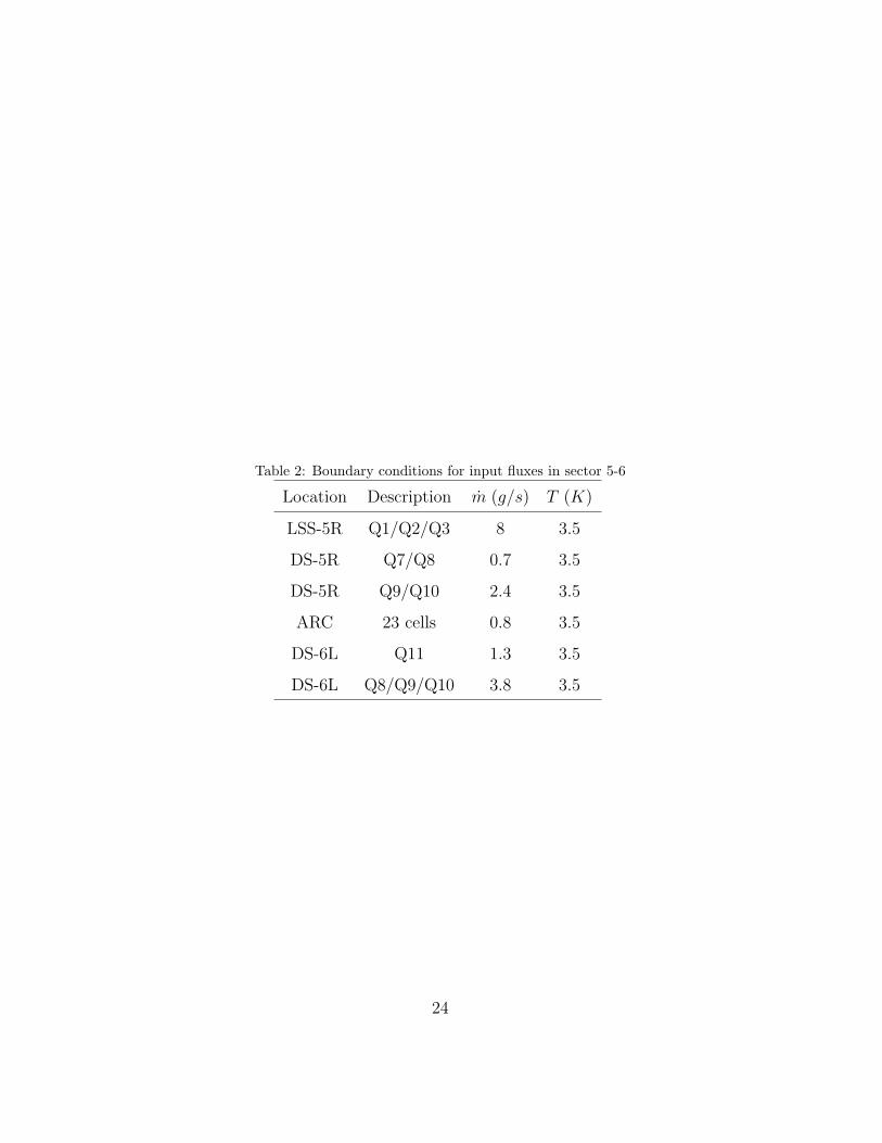
Table 2: Boundary conditions for input fluxes in sector 5-6

Location Description m (g/s) T (K)

LSS-5R Q1/Q2/Q3 8 3.5

DS-5R Q7/Q8 0.7 3.5

DS-5R Q9/Q10 2.4 3.5

ARC 23 cells 0.8 3.5

DS-6L Q11 1.3 3.5

DS-6L Q8/Q9/Q10 3.8 3.5

24