1

MODELING OF THE DYNAMIC RESPONSE OF A FRANCIS TURBINE

Paolo PENNACCHI, Steven CHATTERTON*, Andrea VANIA

Politecnico di Milano, Department of Mechanical Engineering - Via G. La Masa, 1 - 20156 - Milano, Italy.

KEYWORDS: hydroelectric power plant model, pressure waves, Francis turbine.

ABSTRACT The paper presents a detailed numerical model of the dynamic behaviour of a Francis

turbine installed in a hydroelectric plant. The model considers in detail the Francis

turbine with all the electromechanical subsystems, such as the main speed governor, the

controller and the servo actuator of the turbine distributor, and the electrical generator.

In particular, it reproduces the effects of pipeline elasticity in the penstock, the water

inertia and the water compressibility on the turbine behaviour. The dynamics of the

surge tank on low frequency pressure waves is also modeled together with the main

governor speed loop and the position controllers of the distributor actuator and of the

hydraulic electrovalve. Model validation has been made by means of experimental data

of a 75 MW - 470 m hydraulic head - Francis turbine acquired during some starting

tests after a partial revamping, which also involved the control system of the distributor.

NOMENCLATURE ω∆ Deviation of rotational speed in p.u. G∆ Deviation of gate opening in p.u.

tH∆ Deviation of turbine hydraulic head in p.u.

mP∆ Deviation of mechanical power in p.u.

tU∆ Deviation of water velocity in p.u.

pφ Friction energy term of the penstock

cφ Friction coefficient of the tunnel * Corresponding author: email: steven.chatterton@polimi.it, ph: +39 02 23998442, fax: +39 02 23998492

2

ρ Volumetric mass of water

pτ Time constant of the servovalve

0ω Rotational speed in operating condition

pA Penstock area

3, , , ,p t x db b T T T Gains and time constants of the speed controller in operating mode

IC Proportional gain of the gate opening controller

xC Flow gain of the servovalve

pc Wave velocity in the penstock D Damping factor

ckD Diameter of the k-th tunnel (k = 1,2)

pD Penstock diameter eω Rotational speed error in p.u. E Young’s modulus of elasticity of pipe material f Thickness of pipe wall g Gravitational acceleration

0 0,G G Gate opening reference signal and p.u. form G Actual gate opening

0,( )H H Hydraulic head at gate (in operating condition)

0I Current command input of the servovalve J Generator inertia

1k Gain constant of the servovalve

bk Hydraulic cylinder net area constant

fk Friction coefficient of the penstock ,p ik k Gains of the PI speed controller in starting mode

K Bulk modulus of water compression

iK Inertia constant ,u pK K Velocity and power constants

ckL Length of the k-th tunnel (k = 1,2)

pL Penstock length

0,( )m mP P Turbine mechanical power (in operating condition)

tp Water pressure at gate

oilq Oil flow in the hydraulic cylinder

0Q Turbine water flow in operating condition

aT Mechanical starting time

eT Electrical load torque in p.u.

epT Elastic time of the penstock

mT Mechanical torque of the turbine in p.u.

sT Time constant of the surge tank

WcT Starting time of the tunnel

3

WpT Water starting time of the penstock

0,( )U U Water velocity (in operating condition) x Pilot valve spool position

pZ Penstock normalized hydraulic surge impedance

0pZ Hydraulic surge impedance of the penstock

1 INTRODUCTION The accurate dynamic model of turbine units in hydroelectric plants assumes great

importance in case of renewal of turbine components, such as the control and the

actuator systems, or in case of periodic and required inspection of the emergency

systems. In this sense, a model of the entire system prevents dangerous conditions

during the tuning of the control system and provides a reference response for

inspections.

This kind of model could be also used during design phases, for penstock

dimensioning, for the overspeed estimation and for the analysis of new control

strategies of the speed governor.

The first studies about power system of hydro turbines date back to the early 70s,

when a task force on overall plant response was established in order to consider the

effects of power plants on power system stability and to provide recommendations

regarding problems not already investigated. The outcome of this effort has been a first

simple model consisting in transfer functions of the speed governing and the hydro

turbines systems [1].

However, these early models were inadequate to study large variations of power

output and frequency. For instance, they were not reliable in the very low frequency

range, as they did not account for the water mass oscillations between the surge tank

and the reservoir, and at high frequency [2], as they did not reproduce water hammer

effects.

To solve these limitations, some improvements of both turbine and speed control

models were made by the Working Group on Prime Mover and Energy Supply Models

for System Dynamic Performances Studies [3].

In this paper, the authors propose a detailed and complete numerical model of the

dynamic behaviour of a Francis turbine of a hydroelectric plant. The model considers in

detail the Francis turbine with all the electromechanical subsystems, such as the main

4

speed governor, the controller and the servo actuator of the turbine distributor, and the

electrical generator. In particular it reproduces the effects of pipeline elasticity in the

penstock, the water inertia and the water compressibility on the turbine behaviour.

Among the different possible approaches for the pressure wave modelling, the transfer

function method is employed in this paper, allowing testing different closing

manoeuvres of turbine distributor performed by the control system. The dynamics of the

surge tank and of the reservoir on low frequency pressure waves are also modelled

together with the main governor speed loop and the position controllers of the

distributor actuator and of the hydraulic electrovalve.

The proposed model has been successfully validated by means of experimental data

of a 75 MW - 470 m hydraulic head - Francis turbine of a hydroelectric plant, acquired

during some starting tests after a partial revamping, which also involved the control

system of the distributor.

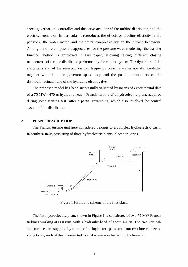
2 PLANT DESCRIPTION

The Francis turbine unit here considered belongs to a complex hydroelectric basin,

in southern Italy, consisting of three hydroelectric plants, placed in series.

ReservoirTunnel 1

Tunnel 2

Surgetank 1

Surgetank 2

Penstock

Turbine 1

Turbine 2

0H

Figure 1 Hydraulic scheme of the first plant.

The first hydroelectric plant, shown in Figure 1 is constituted of two 75 MW Francis

turbines working at 600 rpm, with a hydraulic head of about 470 m. The two vertical-

axis turbines are supplied by means of a single steel penstock from two interconnected

surge tanks, each of them connected to a lake reservoir by two rocky tunnels.

5

The discharged water of the first plant supplies a second reservoir used by the

second plant and so on also for the last plant. The main data of the plant are reported in

Table 1.

Table 1. Data of the hydroelectric central

1cL Tunnel 1 length 4190 m

1cD Tunnel 1 diameter 2.5 m

2cL Tunnel 2 length 4111 m

2cD Tunnel 2 diameter 3.2 m

pL Penstock length 1220 m

pD Penstock diameter 3 m f Thickness of pipe wall 0.020 m 0tQ Penstock overall rated flow 35 m3/s

0H Hydraulic head 440.37-474.43 m 2PD

J Generator inertia PD2 600 103 kgm2

0Q Single turbine rated flow 17-18 m3/s

rP Single turbine electric power 66.3-75.2 MW

0ω Rated speed 600 rpm

A spherical valve, moved by a hydraulic actuator, is placed at the end of the

penstock as shown in Figure 2. This valve operates only during starting, emergency

phases and stopping.

6

Figure 2 Spherical valve at the end of the penstock.

The generator is an 80 MVA-10 kV three-phase synchronous machine running at

600 rpm. The upper part of the exciter system of the generator is shown in Figure 3.

Figure 3 Upper part of the generator exciter system.

7

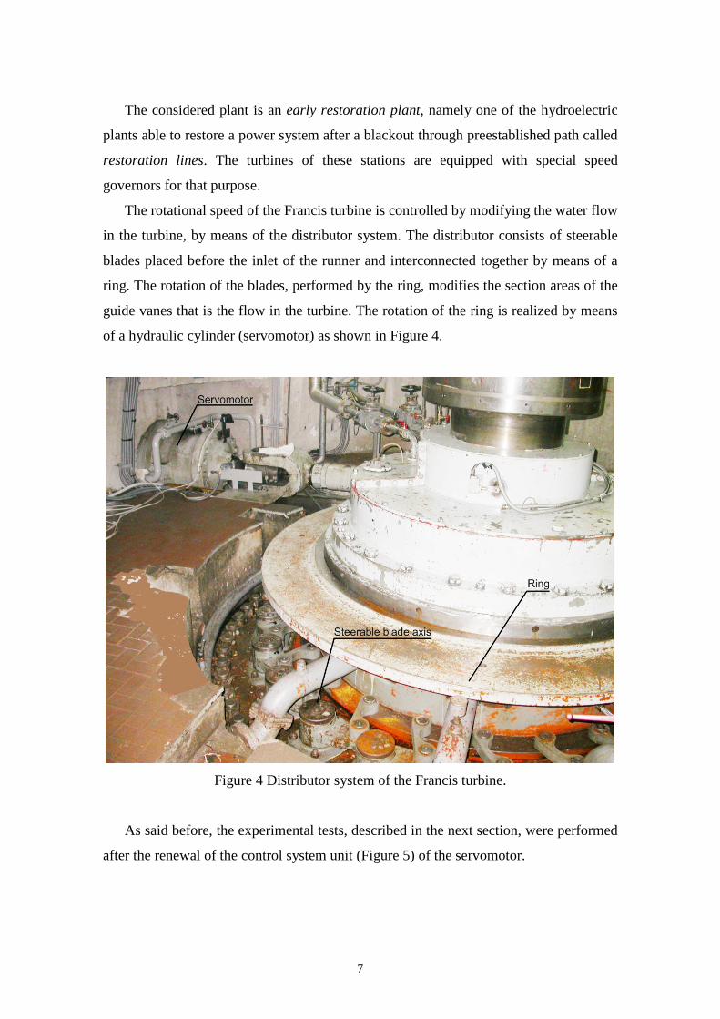
The considered plant is an early restoration plant, namely one of the hydroelectric

plants able to restore a power system after a blackout through preestablished path called

restoration lines. The turbines of these stations are equipped with special speed

governors for that purpose.

The rotational speed of the Francis turbine is controlled by modifying the water flow

in the turbine, by means of the distributor system. The distributor consists of steerable

blades placed before the inlet of the runner and interconnected together by means of a

ring. The rotation of the blades, performed by the ring, modifies the section areas of the

guide vanes that is the flow in the turbine. The rotation of the ring is realized by means

of a hydraulic cylinder (servomotor) as shown in Figure 4.

Figure 4 Distributor system of the Francis turbine.

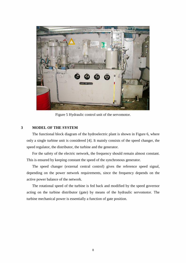
As said before, the experimental tests, described in the next section, were performed

after the renewal of the control system unit (Figure 5) of the servomotor.

8

Figure 5 Hydraulic control unit of the servomotor.

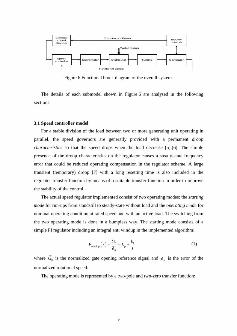
3 MODEL OF THE SYSTEM

The functional block diagram of the hydroelectric plant is shown in Figure 6, where

only a single turbine unit is considered [4]. It mainly consists of the speed changer, the

speed regulator, the distributor, the turbine and the generator.

For the safety of the electric network, the frequency should remain almost constant.

This is ensured by keeping constant the speed of the synchronous generator.

The speed changer (external central control) gives the reference speed signal,

depending on the power network requirements, since the frequency depends on the

active power balance of the network.

The rotational speed of the turbine is fed back and modified by the speed governor

acting on the turbine distributor (gate) by means of the hydraulic servomotor. The

turbine mechanical power is essentially a function of gate position.

9

Servomotor Distributor Turbine Generator

Water supply

Speed controller

Externalspeed

changerElectric network

Rotational speed

Frequency - Power

Figure 6 Functional block diagram of the overall system.

The details of each submodel shown in Figure 6 are analysed in the following

sections.

3.1 Speed controller model For a stable division of the load between two or more generating unit operating in

parallel, the speed governors are generally provided with a permanent droop

characteristics so that the speed drops when the load decrease [5],[6]. The simple

presence of the droop characteristics on the regulator causes a steady-state frequency

error that could be reduced operating compensation in the regulator scheme. A large

transient (temporary) droop [7] with a long resetting time is also included in the

regulator transfer function by means of a suitable transfer function in order to improve

the stability of the control.

The actual speed regulator implemented consist of two operating modes: the starting

mode for run-ups from standstill to steady-state without load and the operating mode for

nominal operating condition at rated speed and with an active load. The switching from

the two operating mode is done in a bumpless way. The starting mode consists of a

simple PI regulator including an integral anti windup in the implemented algorithm:

( ) 0 istarting p

G kF s ke sω

= = +

(1)

where 0G is the normalized gate opening reference signal and eω is the error of the

normalized rotational speed.

The operating mode is represented by a two-pole and two-zero transfer function:

10

( ) ( )( )

0

3

1111

1

x

dtoperating

p x

p

T sT sbGF s

e b T sT sb

ω

+ + = =

+ +

(2)

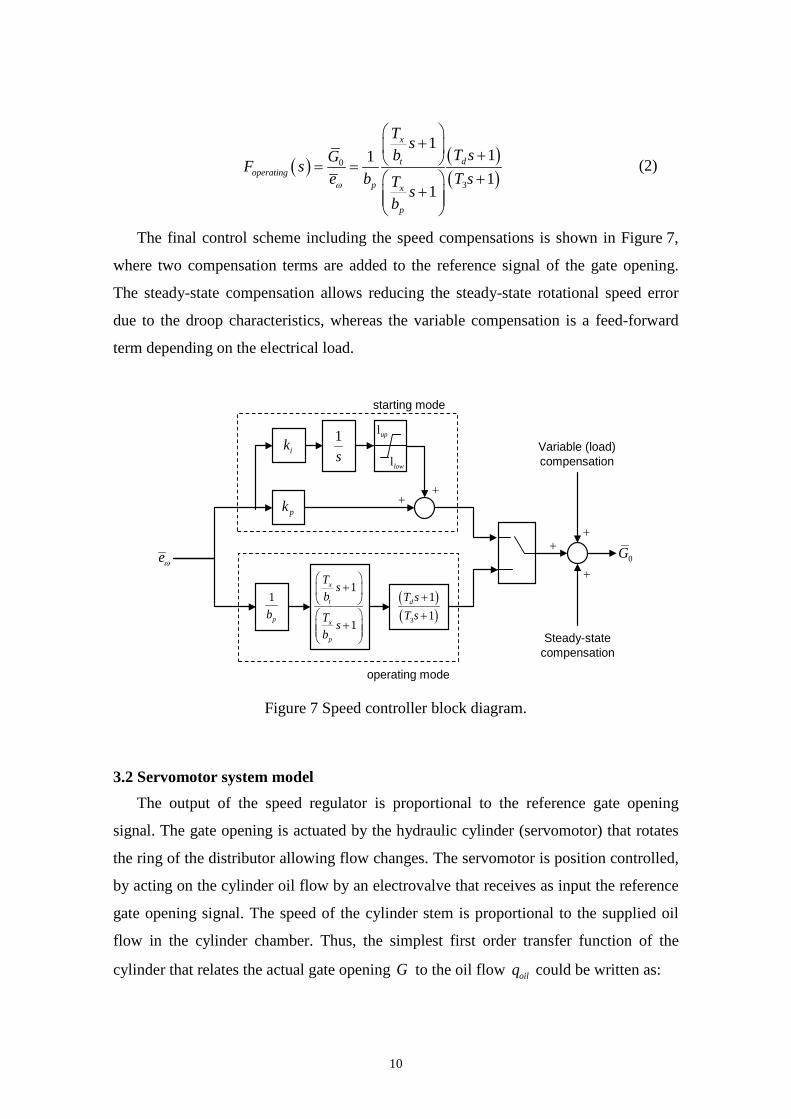
The final control scheme including the speed compensations is shown in Figure 7,

where two compensation terms are added to the reference signal of the gate opening.

The steady-state compensation allows reducing the steady-state rotational speed error

due to the droop characteristics, whereas the variable compensation is a feed-forward

term depending on the electrical load.

( )( )3

11

dT sT s

++

eω

1

pb

1

1

x

t

x

p

T sb

T sb

+

+

operating mode

0G

Steady-statecompensation

Variable (load)compensation

pk

ik 1s llow

lup

++

++

+

starting mode

Figure 7 Speed controller block diagram.

3.2 Servomotor system model The output of the speed regulator is proportional to the reference gate opening

signal. The gate opening is actuated by the hydraulic cylinder (servomotor) that rotates

the ring of the distributor allowing flow changes. The servomotor is position controlled,

by acting on the cylinder oil flow by an electrovalve that receives as input the reference

gate opening signal. The speed of the cylinder stem is proportional to the supplied oil

flow in the cylinder chamber. Thus, the simplest first order transfer function of the

cylinder that relates the actual gate opening G to the oil flow oilq could be written as:

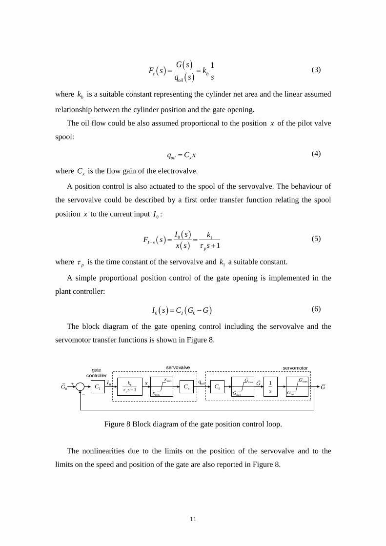
11

( ) ( )( )

1c b

oil

G sF s k

q s s= = (3)

where bk is a suitable constant representing the cylinder net area and the linear assumed

relationship between the cylinder position and the gate opening.

The oil flow could be also assumed proportional to the position x of the pilot valve

spool:

oil xq C x= (4)

where xC is the flow gain of the electrovalve.

A position control is also actuated to the spool of the servovalve. The behaviour of

the servovalve could be described by a first order transfer function relating the spool

position x to the current input 0I :

( ) ( )( )

0 1

1I xp

I s kF sx s sτ− = =

+ (5)

where pτ is the time constant of the servovalve and 1k a suitable constant.

A simple proportional position control of the gate opening is implemented in the

plant controller:

( ) ( )0 0II s C G G= − (6)

The block diagram of the gate opening control including the servovalve and the

servomotor transfer functions is shown in Figure 8.

servovalve

IC 1

1p

ksτ +

minx

maxx

minG

maxG

xCminG

maxG1s0G +

G0I

gatecontroller

−

x oilq G

servomotor

bC

Figure 8 Block diagram of the gate position control loop.

The nonlinearities due to the limits on the position of the servovalve and to the

limits on the speed and position of the gate are also reported in Figure 8.

12

3.3 Turbine model The dynamic behaviour of a hydraulic turbine operating at full load is widely

described by a transfer function that relates the deviation of the output mechanical

power to the deviation of gate opening [5],[8].

The turbine-distributor system is modelled as a valve, where the velocity U of the

water at gate is given by:

uU K G H= (7)

The turbine mechanical power is proportional to the product of pressure and flow:

m pP K HU= (8)

where uK and pK are proportional constants, G is the gate (distributor) opening, and

H is the hydraulic head at the gate.

By linearizing and considering both small displacements about the operating point

and p.u. expressions, it follows:

( )( )

( )

( )

11

1 112

mP s F sG s

F s

+∆

=∆ −

(9)

where ,0m m mP P P∆ = ∆ is the p.u. small deviation of the hydraulic (or mechanical)

power (corresponding to the p.u. mechanical torque), G∆ is the p.u. small deviation of

the gate opening and ( ) ( ) ( )t tF s U s H s= ∆ ∆ is the transfer function that relates the

normalized flow (corresponding to the p.u. water speed) to the normalized hydraulic

head deviation at gate.

3.3.1 Classical model The classical model of the ideal turbine is obtained considering [1],[9]:

( )1

WpT sF s

= − (10)

where WpT is the water starting time (or water time constant) of the penstock at rated

load, that depends on the load conditions. The starting time represents the time required

13

for a total head 0H to accelerate the water in the penstock of length pL from standstill

to the velocity 0U :

0

0

pWp

L UT

gH= (11)

Different values of WpT are used in the model depending on the load condition:

0.65sWpT = for full load condition ( 30, 17.5m sfullQ = ), whereas 0.065sWpT = for the

idling condition ( 30, 1.75m sidlingQ = ).

Equations (9) and (10) describe the behaviour of a simple ideal linear model of

hydraulic turbine for small deviations from steady-state operating point, considering

negligible hydraulic resistance, incompressible water and inelastic penstock pipe.

This model is only a medium-low frequency approximation, with relevant errors in

the high frequency range, because it does not include the water hammer phenomenon.

The model is not also entirely adequate in the very-low-frequency range, as it does not

account for the water-mass oscillations in the tunnel (considered as inelastic) that

connects the surge tank and the reservoir [9].

3.3.2 Detailed model The effects of the travelling waves owing to the elasticity of penstock steel and of

the water compressibility could be considered by means of the method of characteristics

[10],[11] or by means of a transfer function approach. The first method requires the

integration of partial differential equations by means of finite difference method and

allows the time evaluation of the hydraulic head and speed in several point of the

penstock. Instead, the transfer function approach allows only the evaluation of the same

quantities at the turbine level [2].

Considering the presence of the surge tank, the overall and detailed transfer function

to be used in eq. (9) becomes [5]:

( )

( ) ( )( ) ( )

1

1

1 tanh

tanh

eppt

t p p ep

F sT s

ZUF sH F s Z T sφ

+∆

= = −∆ + +

(12)

• ( )1F s is the transfer function that describes the tunnel and surge tank interaction:

14

( )1 21r c Wc

p s c Wc s

H sTF sU sT s T T

φφ

∆ += − =

∆ + + (13)

• WcT is the starting time of the tunnel, sT the time constant of the surge tank and cφ

the friction coefficient of the tunnel;

• epT is the elastic time of the penstock of length pL , diameter pD and area

2 4p pA Dπ= :

pep

p

LT

c= (14)

• pc is the wave velocity in the penstock given by:

pp

gcα

= (15)

• pα considers the water compressibility and the pipe elasticity:

1 pp

Dg

K Efα ρ

= +

(16)

• K is the bulk modulus of water compression, E the Young’s modulus of elasticity

of pipe material and f the thickness of pipe wall;

• pZ is the normalized value of the hydraulic surge impedance of the penstock 0pZ

given by:

00

0p p

QZ ZH

=

(17)

• 0pZ is the hydraulic surge impedance of the penstock:

0p

p

cZ

Ag= (18)

• pφ represents the friction energy term of the penstock:

02p fk Uφ = (19)

The term ( )tanh epT s in eq. (12) could be written as:

15

( )

( )

2

21

2 2

1

11tanh1 2

12 1

ep

ep

epeT s

n

ep T s

ep

n

sTsT

neT se sT

n

π

π

∞

−=

−∞

=

+ − = =

+ + −

∏

∏ (20)

The elastic time is related to the time constant by:

Wp p epT Z T= (21)

The pressure at gate could be easily evaluated by:

( ) 01t tp H H= ∆ + (22)

where tH∆ , depending on the gate opening, could be evaluated by the following

transfer function:

( )( )

112

tp

HF sG F s

∆= =∆ −

(23)

3.3.3 Simplified model Excluding the surge tank and considering in this way only the high-frequency

effects of the water hammer, the following equation should be used [5]:

( ) ( )1

tanht

t p p ep

UF sH Z T sφ

∆= = −∆ +

(24)

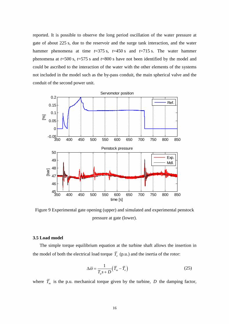
3.4 Experimental penstock pressure All the quantities presented in the previous equation have been evaluated by means

of available data and by experimental data. For instance, the experimental gate opening

described by the servomotor position and the experimental and the simulated penstock

pressure at gate are reported in Figure 9. In particular, the model of the plant including

the turbine, the penstock, the surge tank and the reservoir has been tuned using the

experimental gate opening reported in the upper part of Figure 9 as input of eq. (22) and

evaluating the simulated penstock pressure at gate by means of eq. (23). In the lower

part of Figure 9, both the experimental and the simulated penstock pressures at gate are

16

reported. It is possible to observe the long period oscillation of the water pressure at

gate of about 225 s, due to the reservoir and the surge tank interaction, and the water

hammer phenomena at time t=375 s, t=450 s and t=715 s. The water hammer

phenomena at t=500 s, t=575 s and t=800 s have not been identified by the model and

could be ascribed to the interaction of the water with the other elements of the systems

not included in the model such as the by-pass conduit, the main spherical valve and the

conduit of the second power unit.

350 400 450 500 550 600 650 700 750 800 850-0.05

0

0.05

0.1

0.15

0.2Servomotor position

[%]

Ref.

350 400 450 500 550 600 650 700 750 800 85045

46

47

48

49

50Penstock pressure

time [s]

[bar

]

Exp.Mdl.

Figure 9 Experimental gate opening (upper) and simulated and experimental penstock

pressure at gate (lower).

3.5 Load model The simple torque equilibrium equation at the turbine shaft allows the insertion in

the model of both the electrical load torque eT (p.u.) and the inertia of the rotor:

( )1m e

a

T TT s D

ω∆ = −+

(25)

where mT is the p.u. mechanical torque given by the turbine, D the damping factor,

17

ω∆ the p.u. rotational speed deviation and aT the mechanical starting time. The

mechanical starting time is obtained by the inertia constant 2i aK T= that it is defined

by the ratio of the kinetic energy of the rotor at rated speed 0ω and the rated electrical

power of the generator ( )0VA :

( )20

0

12i

JKVAω

= (26)

Inertia J and damping D change depending on the operating conditions in the

model. For instance, during a closure manoeuvre of the gate, both J and D decrease

due to a reduction of the water present in the runner. The mechanical starting time aT

linearly changes in the range 8.5 9s÷ , whereas D in 0.06 0.1÷ as function of the

normalized gate opening limits 0 1÷ . In this way, the model is linearized about different

steady-state operating points. A change of the damping factor also includes nonlinear

variation of the turbine efficiency for different operating points [12].

Regarding the electrical load, all electrical devices such as the generator, the

transformers and the power network have not been modelled in detail [13]. The

experimental electrical load eT has been used as input in the model simulations.

4 EXPERIMENTAL TESTS

As above mentioned, the considered plant is an early restoration plant and a partial

revamping involved the control system of the distributor. For these reasons, the

experimental data are acquired during some inspection tests of restoring procedures of

the plant control system. In particular, they were aimed at verifying the proper working

of the overall system and have been performed by sending suitable signals to the control

system. For instance, complete closures of the main spherical valve or some

disturbances on the reference speed signal have been simulated.

In particular, two different sets of tests have been carried out only on one of the two

units, with the spherical valve of the second unit completely closed. The first set has

regarded the correct working of the revamped control system of the servomotor,

whereas the latter has been carried out on the overall system in order to test several

operating conditions.

18

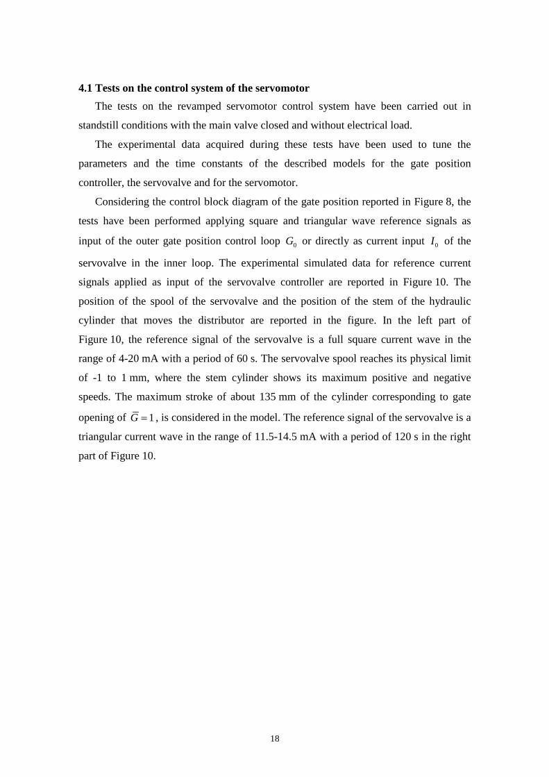
4.1 Tests on the control system of the servomotor The tests on the revamped servomotor control system have been carried out in

standstill conditions with the main valve closed and without electrical load.

The experimental data acquired during these tests have been used to tune the

parameters and the time constants of the described models for the gate position

controller, the servovalve and for the servomotor.

Considering the control block diagram of the gate position reported in Figure 8, the

tests have been performed applying square and triangular wave reference signals as

input of the outer gate position control loop 0G or directly as current input 0I of the

servovalve in the inner loop. The experimental simulated data for reference current

signals applied as input of the servovalve controller are reported in Figure 10. The

position of the spool of the servovalve and the position of the stem of the hydraulic

cylinder that moves the distributor are reported in the figure. In the left part of

Figure 10, the reference signal of the servovalve is a full square current wave in the

range of 4-20 mA with a period of 60 s. The servovalve spool reaches its physical limit

of -1 to 1 mm, where the stem cylinder shows its maximum positive and negative

speeds. The maximum stroke of about 135 mm of the cylinder corresponding to gate

opening of 1G = , is considered in the model. The reference signal of the servovalve is a

triangular current wave in the range of 11.5-14.5 mA with a period of 120 s in the right

part of Figure 10.

19

20 40 60 800

5

10

15

20

I0 - Servovalve current input[m

A]

Ref.

0 50 100 1500

5

10

15

20

I0 - Servovalve current input

Ref.

20 40 60 80-1

-0.5

0

0.5

1x - Servovalve spool position

[mm

]

0 50 100 150-1

-0.5

0

0.5

1x - Servovalve spool position

20 40 60 800

50

100

G - Servomotor position

time [s]

[mm

]

Exp.Mdl.

0 50 100 1500

50

100

G - Servomotor position

time [s]

Exp.Mdl.

Figure 10 Tests on the inner loop of gate position control scheme: 100% square current

wave (left) and triangular wave (right) reference signal as input of the servovalve.

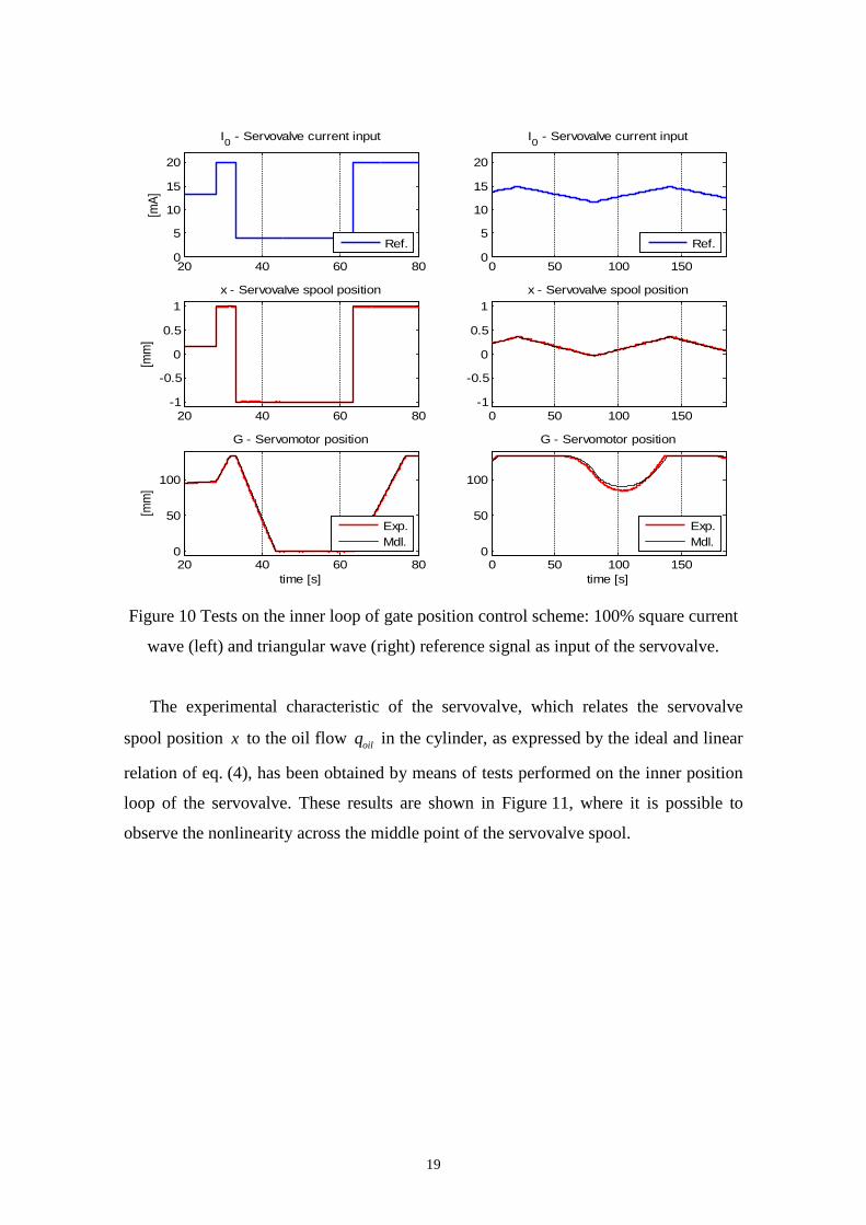
The experimental characteristic of the servovalve, which relates the servovalve

spool position x to the oil flow oilq in the cylinder, as expressed by the ideal and linear

relation of eq. (4), has been obtained by means of tests performed on the inner position

loop of the servovalve. These results are shown in Figure 11, where it is possible to

observe the nonlinearity across the middle point of the servovalve spool.

20

-1 -0.5 0 0.5 1-1

-0.8

-0.6

-0.4

-0.2

0

0.2

0.4

0.6

0.8

q oil

x

Servovalve characteristics

Figure 11 Characteristics curve of the servovalve obtained from experimental data.

4.2 Tests on the overall system The second set of tests has been carried out on the overall system in order to test

several operating conditions:

A) starting procedure from standstill to rated speed, idling electrical load;

B) step reference speed signals at rated speed then stop in idling electrical load;

C) full stop from rated condition (speed and load) closing both to the distributor and

the spherical valve;

D) full load cut out at rated speed.

For the sake of brevity, only the first and the last interesting operation conditions are

reported in the following subsections.

4.2.1 Starting from standstill to rated speed condition The rotational speed, the gate opening and the pressure in the penstock at the

spherical valve are reported in Figure 12, for the starting procedure from standstill to the

rated speed in absence of the electrical load where the speed controller is the PI of

eq. (1). The rotational speed reaches the rated value in about 100 s, where the model

shows a negligible speed overshoot with respect to the experimental data. The rated

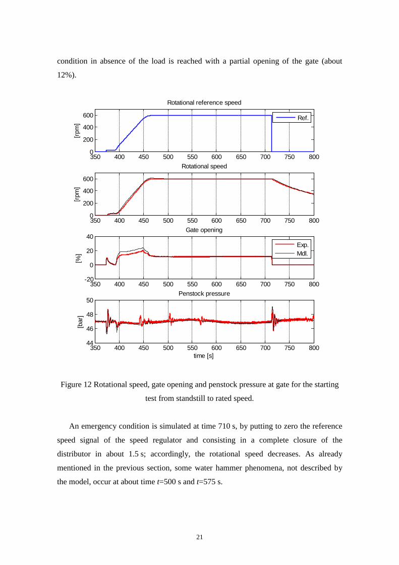
21

condition in absence of the load is reached with a partial opening of the gate (about

12%).

350 400 450 500 550 600 650 700 750 8000

200

400

600

Rotational reference speed

[rpm

]

Ref.

350 400 450 500 550 600 650 700 750 8000

200

400

600

Rotational speed

[rpm

]

350 400 450 500 550 600 650 700 750 800-20

0

20

40Gate opening

[%]

Exp.Mdl.

350 400 450 500 550 600 650 700 750 80044

46

48

50Penstock pressure

time [s]

[bar

]

Figure 12 Rotational speed, gate opening and penstock pressure at gate for the starting

test from standstill to rated speed.

An emergency condition is simulated at time 710 s, by putting to zero the reference

speed signal of the speed regulator and consisting in a complete closure of the

distributor in about 1.5 s; accordingly, the rotational speed decreases. As already

mentioned in the previous section, some water hammer phenomena, not described by

the model, occur at about time t=500 s and t=575 s.

22

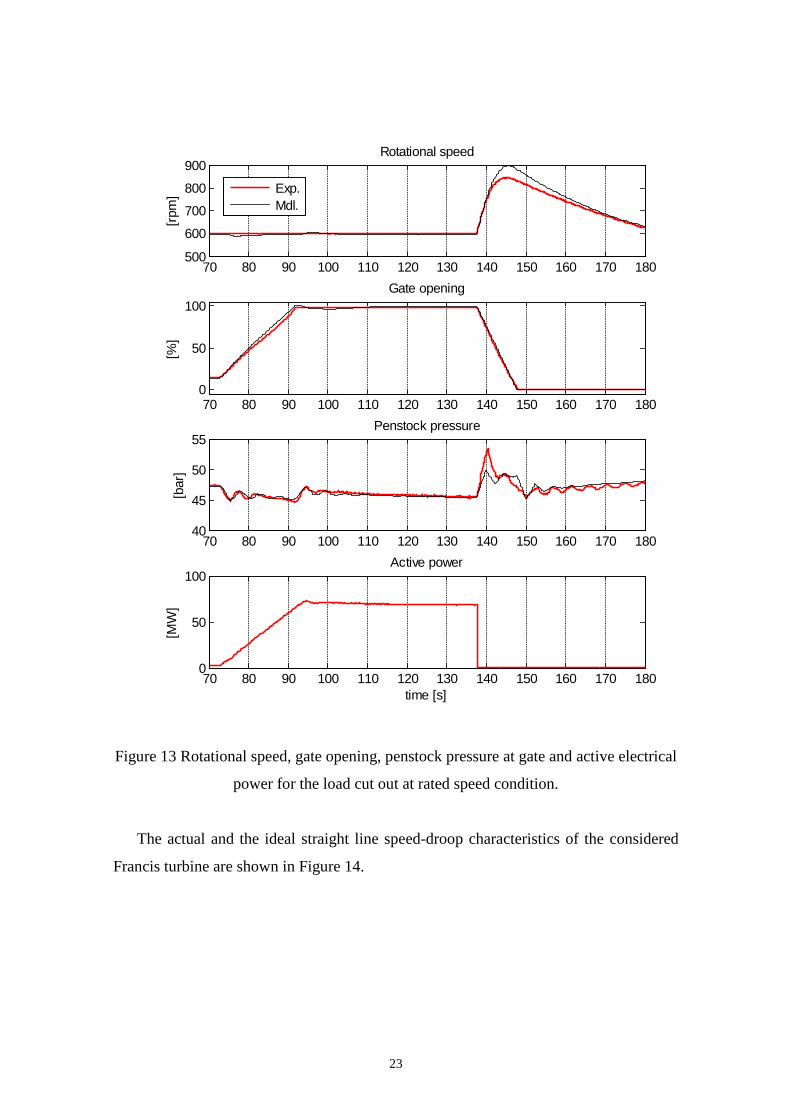
4.2.2 Full load cut out at rated speed condition The electrical load cut out at rated speed is analysed in this case. This condition is

extremely dangerous because a turbine overspeed occurs, as shown in the upper

diagram of Figure 13, where the rotational speed, the gate opening, the penstock

pressure and the active electrical power are also reported. The electrical load is linearly

applied starting from time t=72 s till t=95 s and is completely removed at time t=137 s

as appears from the last diagram of the figure, by disconnecting the generator from the

power network. The experimental overspeed is about 40% whereas the simulated one is

about 50% of the rated speed. The difference between the experimental and the

simulated overspeed could be ascribed to the nonlinearity of the damping of the system

described by eq. (25).

23

70 80 90 100 110 120 130 140 150 160 170 180500

600

700

800

900Rotational speed

[rpm

]

Exp.Mdl.

70 80 90 100 110 120 130 140 150 160 170 1800

50

100Gate opening

[%]

70 80 90 100 110 120 130 140 150 160 170 18040

45

50

55Penstock pressure

[bar

]

70 80 90 100 110 120 130 140 150 160 170 1800

50

100Active power

time [s]

[MW

]

Figure 13 Rotational speed, gate opening, penstock pressure at gate and active electrical

power for the load cut out at rated speed condition.

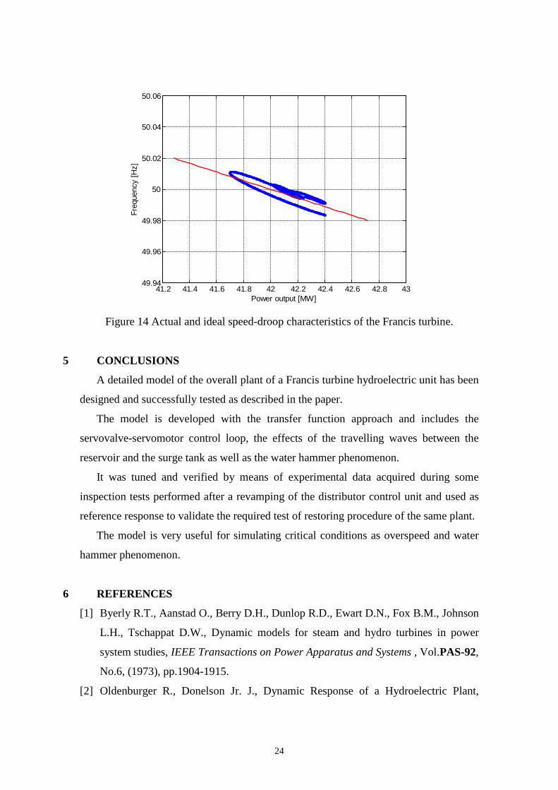
The actual and the ideal straight line speed-droop characteristics of the considered

Francis turbine are shown in Figure 14.

24

41.2 41.4 41.6 41.8 42 42.2 42.4 42.6 42.8 4349.94

49.96

49.98

50

50.02

50.04

50.06

Freq

uenc

y [H

z]

Power output [MW] Figure 14 Actual and ideal speed-droop characteristics of the Francis turbine.

5 CONCLUSIONS

A detailed model of the overall plant of a Francis turbine hydroelectric unit has been

designed and successfully tested as described in the paper.

The model is developed with the transfer function approach and includes the

servovalve-servomotor control loop, the effects of the travelling waves between the

reservoir and the surge tank as well as the water hammer phenomenon.

It was tuned and verified by means of experimental data acquired during some

inspection tests performed after a revamping of the distributor control unit and used as

reference response to validate the required test of restoring procedure of the same plant.

The model is very useful for simulating critical conditions as overspeed and water

hammer phenomenon.

6 REFERENCES

[1] Byerly R.T., Aanstad O., Berry D.H., Dunlop R.D., Ewart D.N., Fox B.M., Johnson

L.H., Tschappat D.W., Dynamic models for steam and hydro turbines in power

system studies, IEEE Transactions on Power Apparatus and Systems , Vol.PAS-92,

No.6, (1973), pp.1904-1915.

[2] Oldenburger R., Donelson Jr. J., Dynamic Response of a Hydroelectric Plant,

25

Transaction of the American Institute of Electrical Engineers, Vol.81, No.3 (1962),

pp.403-418.

[3] Working Group on Prime Mover, Hydraulic turbine and turbine control models for

system dynamic studies, IEEE Transactions on Power System, Vol.7, No.1 (1992),

pp.167-179.

[4] De Jaeger E., Janssens N., Malfliet B., Van De Meulebroeke F., Hydro Turbine

model for system dynamic studies, IEEE Transactions on Power Systems, Vol.9,

No.4, (1994), pp.1709-1715.

[5] Kundur P., Power system stability and control, (1994), EPRI Editors.

[6] Schleif F.R., Wilbor A.B., The coordination of hydraulic turbine governors for

power system operations, IEEE Transactions on Power Apparatus and Systems,

Vol.PAS-85. No.7, (1965), pp.750-758.

[7] Undrill J.M., Woodward J.L., Nonlinear hydro governing model and improved

calculation for determining temporary droop, IEEE Transactions on Power

Apparatus and Systems, Vol.PAS-86, No.4, (1967), pp.443-453.

[8] Hannett L.N., Feltes J.W., Fardanesh B., Field tests to validate hydro turbine-

governor model structure and parameters, IEEE Transactions on Power System,

Vol.9, No.4, (1994), pp.1744-1751.

[9] Ramey D.G., Skooglund J.W., Detailed hydrogovernor representation for system

stability studies, IEEE Transactions on Power Apparatus and Systems, Vol.PAS-

89. No.1, (1970), pp.106-112.

[10] Larock B.E., Jeppson R.W., Watters G.Z., Hydraulics of pipeline system, CRC

Press, (2000).

[11] Afshar M.H., Rohani M., Water hammer simulation by implicit method of

characteristic, International Journal of Pressure Vessels and Piping, Vol.85, No.12,

(2008), pp.851-859.

[12] Tzuu Bin Ng, Walker G.J., Sargison J.E., Modelling of transient behaviour in a

Francis turbine power plant, 15th Australian Fluid Mechanics Conference, (2004),

pp.1-4.

[13] Okou F.A., Akhrif O., Dessaint L., A robust nonlinear multivariable controller for

multimachine power systems, Proceedings of the 2003 American Control

Conference, Vol.3, (2003), pp.2294-2299.

26

Figure Captions:

Figure 1 Hydraulic scheme of the first plant.

Figure 2 Spherical valve at the end of the penstock.

Figure 3 Upper part of the generator exciter system.

Figure 4 Distributor system of the Francis turbine.

Figure 5 Hydraulic control unit of the servomotor.

Figure 6 Functional block diagram of the overall system.

Figure 7 Speed controller block diagram.

Figure 8 Block diagram of the gate position control loop.

Figure 9 Experimental gate opening (upper) and simulated and experimental penstock

pressure at gate (lower).

Figure 10 Tests on the inner loop of gate position control scheme: 100% square current

wave (left) and triangular wave (right) reference signal as input of the servovalve.

Figure 11 Characteristics curve of the servovalve obtained from experimental data.

Figure 12 Rotational speed, gate opening and penstock pressure at gate for the starting

test from standstill to rated speed.

Figure 13 Rotational speed, gate opening, penstock pressure at gate and active electrical

power for the load cut out at rated speed condition.

Figure 14 Actual and ideal speed-droop characteristics of the Francis turbine.

27

Table Caption:

Table 1. Data of the hydroelectric central