Modeling of Selenium for the San Diego Creek Watershed and ... › of › 2009 › 1114 › of2009-1114.pdf · The San Diego Creek watershed and Newport Bay in southern California

U.S. Department of the InteriorU.S. Geological Survey

Open-File Report 2009-1114

U.S. Department of the InteriorU.S. Geological Survey

Open-File Report 2009-1114

Modeling of Selenium for the San Diego Creek Watershed and Newport Bay, California

Cover Photos: In order from top, space radar image of Orange County, California, NASA, 2006 [http://visibleearth.nasa.gov]; birds: curlew, skimmer, pelican, and mallard; Upper Newport Bay Ecological Reserve; middle portion of Newport Bay, Lower Newport Bay, California State University, Long Beach, College of Natural Science and Mathematics [http://www.cnsm.csulb.edu].

Cover art by Jeanne DiLeo, USGS, Menlo Park, Calif.

http://visibleearth.nasa.gov/

http://www.cnsm.csulb.edu/

Modeling of Selenium for the San Diego Creek Watershed and Newport Bay, California

By Theresa S. Presser and Samuel N. Luoma

Open-File Report 2009-1114 U.S. Department of the Interior U.S. Geological Survey

ii

U.S. Department of the Interior KEN SALAZAR, Secretary

U.S. Geological Survey Suzette M. Kimball, Acting Director

U.S. Geological Survey, Reston, Virginia 2009

For product and ordering information: World Wide Web: http://www.usgs.gov/pubprod Telephone: 1-888-ASK-USGS

For more information on the USGS—the Federal source for science about the Earth, its natural and living resources, natural hazards, and the environment: World Wide Web: http://www.usgs.gov Telephone: 1-888-ASK-USGS

Suggested citation: Presser, T.S., and Luoma, S.N., 2009, Modeling of selenium for the San Diego Creek watershed and Newport Bay, California: U.S. Geological Survey Open-File Report 2009-1114, 48 p. [http://pubs.usgs.gov/of/2009/1114/].

Any use of trade, product, or firm names is for descriptive purposes only and does not imply endorsement by the U.S. Government.

Although this report is in the public domain, permission must be secured from the individual copyright owners to reproduce any copyright the material contained within this report.

http://www.usgs.gov/pubprod�

http://www.usgs.gov/�

http://pubs.usgs.gov/of/2009/1114/�

iii

Contents Abstract ........................................................................................................................................... 1 Introduction ..................................................................................................................................... 1 Conceptual Models .......................................................................................................................... 3 Partitioning Coefficient (Kd) .............................................................................................................. 5

San Diego Creek Watershed ....................................................................................................... 5 Newport Bay ................................................................................................................................ 7

Trophic Transfer Factors (TTFs) ...................................................................................................... 8 Invertebrates ................................................................................................................................ 9 Fish............................................................................................................................................ 10 Birds .......................................................................................................................................... 10

Modeling........................................................................................................................................ 11 Scenarios................................................................................................................................... 11 Validation ................................................................................................................................... 12

Summary ....................................................................................................................................... 12 Acknowledgments ......................................................................................................................... 12 References Cited ........................................................................................................................... 13 Tables ........................................................................................................................................... 19 Figures .......................................................................................................................................... 44

iv

Figures Figure 1. Schematic of San Diego Creek watershed and Newport Bay. The Upper Newport Bay Ecological Reserve is shown. .................................................................................................. 44 Figure 2. Conceptual model for the San Diego Creek watershed illustrating linked factors that determine the effects of Se on ecosystems. ................................................................................... 45 Figure 3. Conceptual model for the upper Newport Bay illustrating linked factors that determine the effects of Se on ecosystems. ................................................................................... 46 Figure 4. Conceptual model for the lower Newport Bay illustrating linked factors that determine the effects of Se on ecosystems. .................................................................................................... 47 Figure 5. Extrapolation of dissolved Se at 15.1 ppt to 0 ppt. Data from transect of the upper Newport Bay from the mouth of San Diego Creek into the upper bay (CH2MHILL, 2008). .............. 48

Tables Table 1. Total water-column Se concentrations and Se speciation for the San Diego Creek watershed. ...................................................................................................................................... 19 Table 2a. Dissolved or total water-column Se concentrations; Se concentrations in bed sediment and algae; and calculated Kds for the San Diego Creek watershed (freshwater sites). .... 20 Table 2b. Statistics for calculated Kds based on table 2a data. ....................................................... 21 Table 3. Dissolved water-column Se concentrations and speciation for the Newport Bay estuary. .......................................................................................................................................... 22 Table 4. Water-column and suspended particulate Se concentrations in Upper Newport Bay in a transect from the near the mouth of San Diego Creek into the upper bay to salinities of 33.1 ppt. ................................................................................................................................................. 22 Table 5. Water-column and sediment Se concentrations and calculated Kds in a gradient from landward to seaward in Newport Bay. ............................................................................................. 22 Table 6. Experimental data for invertebrate physiological factors and calculated kinetic TTFs for invertebrates. ............................................................................................................................ 23 Table 7. Field-derived TTFs for invertebrates from field datasets (temporally and spatially matched data-pairs), with experimentally derived TTFs given for comparison ................................ 24 Table 8. Invertebrate Se concentrations for the San Diego Creek watershed. ............................... 25 Table 9. Invertebrate Se concentrations for Newport Bay. .............................................................. 25 Table 10. Selected particulate Se concentration and a comparison of calculated invertebrate TTFs for the San Diego Creek watershed and invertebrate TTF derived from the literature. ........... 26 Table 11. Experimentally or field derived TTFs for fish. .................................................................. 27 Table 12. Fish Se concentrations for the San Diego Creek watershed. .......................................... 28 Table 13. Invertebrate and fish Se concentrations for San Diego Creek watershed and derivation of watershed-specific TTFs for fish. ................................................................................ 29 Table 14. Invertebrate and fish Se concentrations for Newport Bay and derivation of bay-specific TTFs for fish. ..................................................................................................................... 30 Table 15. Mean and ranges for bird egg Se concentrations for the San Diego Creek watershed. ...................................................................................................................................... 31 Table 16. Mean and ranges for bird egg Se concentrations for Upper Newport Bay ....................... 31

v

Table 17. Calculated TTFs from laboratory mallard studies; the endpoint is reduced hatchability in eggs (see Ohlendorf, 2003 for complete dataset). .................................................... 31 Table 18. Modeled Se exposure for the San Diego Creek watershed and Newport Bay. ................ 32 Table 19. Modeled Se exposure for the San Diego Creek watershed and Newport Bay. ............... 33 Table 20. Modeled Se exposure for the San Diego Creek watershed and Newport Bay. ................ 34 Table 21. Generalized modeled Se exposure scenarios for the watershed based on protection for fish. ........................................................................................................................................... 36 Table 22. Generalized modeled exposure scenarios for the watershed based on protection of birds. .............................................................................................................................................. 37 Table 23. Model validation for Newport Bay showing predicted and observed fish Se concentrations. ............................................................................................................................... 38 Table 24. Model validation for bay showing (1) predicted and observed fish Se concentrations and (2) predicted and observed bird egg Se concentrations. ........................................................ 39 Table 25. Model validation for bay showing predicted and observed bird egg Se concentrations. ............................................................................................................................... 40 Table 26. Model validation for watershed showing (1) predicted and observed invertebrate Se concentrations and (2) predicted and observed bird egg Se concentrations. ................................. 41 Table 27. Model validation for watershed showing (1) predicted and observed fish Se concentrations and (2) predicted and observed bird egg Se concentrations. .................................. 42 Table 28. Model validation for watershed showing predicted and observed bird egg Se concentrations. ............................................................................................................................... 43

1

Modeling of Selenium for the San Diego Creek Watershed and Newport Bay, California By Theresa S. Presser and Samuel N. Luoma

Abstract The San Diego Creek watershed and Newport Bay in southern California are

contaminated with selenium (Se) as a result of groundwater associated with urban development overlying a historical wetland, the Swamp of the Frogs. The primary Se source is drainage from surrounding seleniferous marine sedimentary formations. An ecosystem-scale model was employed as a tool to assist development of a site-specific Se objective for the region. The model visualizes outcomes of different exposure scenarios in terms of bioaccumulation in predators using partitioning coefficients, trophic transfer factors, and site-specific data for food-web inhabitants and particulate phases. Predicted Se concentrations agreed well with field observations, validating the use of the model as realistic tool for testing exposure scenarios. Using the fish tissue and bird egg guidelines suggested by regulatory agencies, allowable water concentrations were determined for different conditions and locations in the watershed and the bay. The model thus facilitated development of a site-specific Se objective that was locally relevant and provided a basis for step-by-step implementation of source control.

Introduction Understanding the biotransfer of selenium (Se) is essential for evaluating the effects of Se on ecosystem resources. The linked approach presented in the San Francisco Bay-Delta Selenium Model (Presser and Luoma, 2006) considers progressive modeling of Se through water-column loads, concentrations, and speciation; particulate matter transformation and bioavailability; the biodynamics of bioaccumulation in prey; and trophic transfer to predators. This approach can conceptualize and model Se exposure through site-specific food webs and determine the vulnerability of predator species in an ecosystem. This approach also can be used to generate forecasts of how Se moves through a watershed and estuary based on selected management and regulatory options.

2

Groundwater- and wastewater-related discharges of Se within the San Diego Creek watershed have the potential to adversely affect surface waters and, hence, habitats within the watershed and Newport Bay (fig. 1) (U.S. Environmental Protection Agency, 2002). In 2004, the California Santa Ana Regional Water Quality Control Board issued a revised National Pollutant Discharge Elimination System permit regulating groundwater-related discharges in the watershed (California Santa Ana Regional Water Quality Control Board, 2004). This specific revised regulatory approach addressed (1) the presence of Se and nitrogen and (2) the ability to comply with established Total Maximum Daily Load requirements for impaired water bodies (that is, San Diego Creek and Newport Bay) (U.S. Environmental Protection Agency, 2002). This action initiated an alternative compliance approach allowing stakeholders to participate in Work Groups to develop and implement a comprehensive Work Plan to address Se and nitrogen. This process included Federal agencies (U.S. Environmental Protection Agency, U.S. Fish and Wildlife, U.S. Geological Survey), State and County agencies (California State and Regional Boards; California Department of Fish and Game; County of Orange), and three consulting groups (CH2M Hill, RBF Consulting, and Larry Walker Associates) working cooperatively as the Resource and Regulatory Agency Group with the regulated community to develop a site-specific Se objective to integrate into a watershed scale management strategy for Se (California County of Orange, 2006a; Larry Walker Associates and CH2M Hill, 2007; California Nitrogen and Selenium Management Program, 2006a). A primary task included in the development of the site-specific Se objective was the adaptation of the San Francisco Bay-Delta Selenium Model to the San Diego Creek watershed and Newport Bay. The modeling would translate selected tissue guidelines for predators (that is, whole-body fish tissue and bird egg tissue) to dissolved Se concentrations at chosen sites in the watershed. The dissolved Se concentrations would then facilitate calculation of Total Maximum Daily Load Se requirements for the watershed (U.S. Environmental Protection Agency, 2002).

This report is supplemental to the larger effort of justifying, deriving, and implementing a site-specific Se objective for San Diego Creek watershed and Newport Bay (California Santa Ana Regional Water Quality Control Board, 2004). In that regard, this report is written mainly for a specific audience that has considerable knowledge of the watershed and has participated in Resource and Regulatory Agency Group and Work Group meetings from 2007 to 2009. In addition to this project report, a report is planned that further details and justifies the approach for ecosystem-scale modeling of Se.

This report (1) designs conceptual models for the San Diego Creek watershed and Newport Bay; (2) derives and justifies partitioning coefficients (Kds) and trophic transfer factors (TTFs) used in modeling of the watershed and bay; (3) models different food-web scenarios to elucidate Se exposure within the watershed and bay; and (4) compares predicted Se concentrations to modeled Se concentrations (that is, validation). The work presented here shows the nature of a cooperative iterative process resulting in site-specific regulation and the evolution of our modeling effort. During this time, additional field data became available, data gaps were addressed, feedback was given, guidelines were developed, and revised exposure scenarios were completed. Thus, this report, in addition to illustrating modeling of Se for the watershed and bay, serves as a record to support decision-making within the larger group of resource and regulating agencies.

3

From a scientific perspective, this watershed-scale project illustrates the importance of ecosystem knowledge, especially ecology, for successful Se modeling.

Conceptual Models A generalized schematic of the San Diego Creek watershed and Newport Bay is presented in Figure 1. The watershed is in an urban setting that is intensively developed (93 percent urban uses; 7 percent agricultural uses, including plant nurseries). Newport Bay is an important southern California estuary that is an ecological reserve in the upper portion and a developed marina for recreational boating and fishing in the lower portion. Figure 1 shows the boundaries of historical marshes (Swamp of the Frogs and an ephemeral lake), and these areas overlay aquifers containing the most elevated Se concentrations (Hibbs and Lee, 2000; Meixner and others, 2004). Geologic Se sources are implicated for the watershed including the surrounding Monterey Formation (Piper and Isaacs, 1994). Ninety-six percent of Se loading is estimated to be from groundwater sources in the watershed (California Nitrogen and Selenium Management Program, 2006b; 2009). Drains and drainage channels are important parts of the hydrology of the watershed because of the presence of a high ground water table (Hibbs and Lee, 2000; Meixner and others, 2004).

Sites for modeling (Larry Walker Associates Inc. and CH2M Hill, 2007) within the San Diego Creek watershed and Newport Bay include:

• marsh drains (drains within the area historically designated as the Swamp of the Frogs);

• non-marsh drains (drains outside the area of the historical swamp); • upper and lower San Diego Creek (SDC); • upper and lower Peters Canyon Wash (PCW); • Irvine Ranch Water District (IRWD) off-channel wetlands; • University of California at Irvine (UCI) off-channel wetlands; and • Upper and Lower Newport Bay.

Some data exist for other freshwater drainages to the bay [for example, Santa Ana Delhi Channel (SADC), Big Canyon Wash], but these sites are not included in the final exposure analysis.

Aquatic habitat categories within the area are: riparian channels and pools; control basins; freshwater wetlands; salt marsh; tidal mudflat; estuarine open-water; and marine open-water. The quality of the habitats varies, as does the potential for Se interaction (for example, low habitat value and high Se exposure in some marsh drains). Many of the habitat components are highly engineered and managed to serve several purposes, including treatment for nitrogen and phosphorus and sediment control (for example, in-channel or off-channel wetlands; detention basins in lower San Diego Creek).

The Upper Newport Bay Ecological Reserve and the bay itself (fig. 1) are important stopovers for birds on the Pacific Flyway. Threatened or endangered bird species include the light-footed clapper rail (Rallus longirostris levipes), California brown pelican

4

(Pelecanus occidentalis californicus), and California least tern (Sterna antillarum browni) (Sutula and others, 2005; Allen and others, 2008). Bird species of concern in California are osprey (Pandion haliaetus), double-crested cormorant (Phalacrocorax auritus), elegant tern (Thalasseus elegans), black skimmer (Rhynchops niger), and California gull (Larus californicus). Forage fish species that serve as food for birds include killifish, goby, juvenile halibut, sculpin, and topsmelt (Allen and others, 2004). Larger predatory fish species include sea basses, halibut, sand bass, croaker, and jacksmelt. Shellfish sampling of bivalves showed 24 species of bivalves, with the lower bay supporting more species (California County of Orange, 2004). However, lack of previously available commercial species has deterred studies to evaluate the suitability of existing bay habitats and water quality for renewal of a shellfish industry. Several organic chemicals, including modern pesticides (diazinon, chlorpyrifos) and legacy pesticides (DDT, Chlordane), as well as heavy metals (cadmium, copper, lead, zinc, and mercury) also are of concern in the watershed and bay and may have affected the status of specific food webs and their inhabitants (U.S. Environmental Protection Agency, 2002).

Conceptual Se models for the San Diego Creek watershed and Newport Bay are based on the approach of Presser and Luoma (2006) (figs. 2-4). Important components of food webs identified from site-specific monitoring data (CH2M Hill, 2008a) for the freshwater portions of the watershed are:

• invertebrates: aquatic insect, crayfish, clam, snail, worm, leech. • fish: minnow, sunfish, carp shiner, crappie, catfish, bass, mosquitofish. • birds: avocet, stilt, rail, killdeer, coot, mallard, grebe.

Important components of food webs identified from site-specific monitoring data (CH2M Hill, 2008a) for the estuarine and marine portions of bay are:

• invertebrates: amphipod, isopod, clam, mussel, crab, snail. • fish: mullet, killifish, goby, anchovy, sandbass, turbot, halibut, sculpin, perch,

topsmelt. • birds: avocet, stilt, rail, killdeer, tern, skimmer.

Some species not represented in the collected species (for example, polychaetes) were modeled because of implications for past and future food webs.

Datasets compiled for modeling are food-web-specific and include Se data for the water column (dissolved or total Se); particulate phases; invertebrates; fish (whole-body); birds (egg); and, when available, dissolved Se speciation and salinity (CH2M Hill, 2008a). These datasets are limited to data that are temporally and spatially matched [that is, datasets gathered across media (water, particulate material, invertebrates, fish and/or bird tissue) and during a constrained time period]. Summaries of the data are presented in this report, with extensive documentation available in the spreadsheet datasets that are part of the site-specific Se objective process (CH2M Hill, 2008a). Data are sorted according to seasonal conditions (wet season, November through April, and dry season, May through October). However, the small number of data for prey and predators precluded conclusions based on season. All solids data are given in dry weight (dw).

5

Partitioning Coefficient (Kd) San Diego Creek Watershed

Partitioning of Se between water and particulate material is a dynamic biogeochemical process. Because of the biology involved, it is complex to model (that is, geochemical modeling misses major biological processes). At any point in time and space, Se partitioning can be described by a distribution coefficient, which is the ratio

Kd = Se concentrations in particulate (µg/kg dw) / Se concentrations in water (µg/L).

Note that particulate Se concentrations are usually expressed as µg/g dw. These units must be converted to µg/kg dw to make the particulate concentrations comparable to water concentrations. Presser and Luoma (2006) explained this coefficient in detail and presented data from the literature showing the wide range of distribution coefficients (Kd’s) that occurred in different environments. They recognized that the use of Kd is an operational, descriptive choice for characterizing Se dynamics in an environment. As a practical measure Kd is very useful, but there are limits to its interpretation in terms of describing and quantifying phase transformation processes (Presser and Luoma, 2006).

A major factor determining the magnitude of the partitioning coefficient is Se speciation in the water column (Presser and Luoma, 2006). Dissolved Se can exist as selenate, selenite, and organo-Se. Selenium speciation also differs in nature with the character of the input to a water body and the residence time in the water body. For example, Se often enters a stream (for example, San Diego Creek) as selenate. If that stream flows into a wetland and is retained in a wetland (that is, in-stream water becomes off-stream water) with sufficient residence time, then recycling of Se may occur. During recycling, some selenate is taken up by bacteria and/or plants and converted to selenite and organo-Se. These reduced species then are released back to the water as these organisms die and decay. The more recycling, the more selenite and organo-Se are produced. Neither of the latter forms can be re-oxidized to selenate; that reaction takes hundreds of years (Cutter and Bruland, 1984). Therefore, the net outcome of recycling in a watershed is a gradual buildup of selenite and organo-Se in the water. This process is evidenced in the San Diego Creek watershed by a small increase in selenite (21 to 25 percent) toward the downstream end of the system, 39-100 percent selenite in watershed wetlands, and as much as 78 percent selenite in the estuary (table 1).

Reactions between particles and dissolved Se are dominated by biological uptake into bacteria, plants, and their decaying debris termed detritus. Selenate is the least reactive of the three forms of dissolved Se in generating particulate material. Thus, if selenate is the only form of Se, then the Kd tends to be low. This condition reflects low Se concentrations on particulate material compared to Se concentrations in the water column. As selenite concentrations increase (even if that increase is small) the ratio begins to increase. In the case here, as the San Diego Creek watershed changes from freshwater to the saline water of the estuary and bay, residence time increases, recycling increases, and eventually the ratio of particulate to dissolved Se can be extremely high as Se is stripped from the water column with increasing effectiveness.

6

Presser and Luoma (2006) discussed several studies that supported the link between speciation and partitioning coefficient; however, several additional studies are included in this report. Calculations using data from laboratory microcosms and experimental ponds show speciation-specific Kds of 140-493 for selenate; 720-2,800 when an elevated proportion of selenite exists; and 12,197-36,300 for 100-percent dissolved seleno-methionine uptake into algae or periphyon (Besser and others, 1989; Graham and others, 1992; Kiffney and Knight, 1990). These ranges are consistent with the general ranges for Kd used by Presser and Luoma (2006) for modeling of the San Francisco Bay-Delta Estuary when they developed scenarios based on several possible fates for Se. These ranges also are consistent with the full range for Se in the San Diego Creek watershed and Newport Bay.

The Kd also can be influenced by the type of material in the sediment, although to a lesser degree than by speciation. For example, field data for Luscar Creek in Alberta, Canada, show a hierarchy of Se concentrations: 2.4 µg/g dw in sediment, 3.2 µg/g dw in biofilm, and 5.5 µg/g dw for filamentous algae (Casey, 2005). Using these concentrations with a field-measured dissolved Se concentration of 10.7 µg/L yields Kds of 224, 299, and 514 respectively, with an average Kd of 346. Similarly, field data for a slough tributary to the San Joaquin River, California, show a hierarchy of Se concentrations: 0.47 µg/g dw in sediment, 2.4 µg/g dw in algae, and 7.9 µg/g dw in detritus (Saiki and others, 1993). Using these concentrations with a field-measured dissolved Se concentration of 13 µg/L yields Kds of 36, 185, and 608 respectively, with an average Kd of 276.

Interpretation of particulate Se concentrations should take into consideration, where possible, the nature of the particulate material. Bed sediments are the least desirable choice for calculating Kd, especially if the sediments vary from sand to fine-grained material among the samples. Sandy sediments dilute concentrations with a high mass of inorganic material and may yield Kds that are anomalously low. On the other hand, bed sediments samples are the most traditional type of sample to collect; and Se concentrations in bed sediment are commonly all that are available. In that case, these data are used for determination of Kd. Further operational choices include comparison of one consistent type of material among locations or comparison of an average of the different types of materials (that is, all relevant particulate phases). In practical terms however, modelers usually have to work with the particulate Se data that are available and try to find ways to both minimize the influences caused by particle type and capture the influences of changes in speciation. This is the approach taken below.

Several approaches are possible in choosing a Kd(s) for the San Diego Creek watershed. The dataset for Se concentrations in the water column is extensive, but a smaller dataset exists for particulate Se concentrations (CH2M Hill, 2008a). Table 1 is a summary of total water-column Se concentrations and the percentages of dissolved selenite for the watershed during the dry season. The datasets for water and sediment data pairs were more numerous for the dry season than for the wet season. Table 2a shows a summary of available Se concentrations for bed sediment and algae samples collected in the same place and at the same time as the water-column samples (that is, matched samples). The 75th percentile values for all data collected at each of the sites also are shown. Use of a 75th percentile value was chosen by the Resource and Regulatory Agency Group as a

7

useful statistical representation for the data. The location-specific Kds are calculated from these data and are shown in table 2a. Table 2a was assembled at the request of the Resource and Regulatory Agency Group for the purpose of illustrating the basis for decisions (and the uncertainty around those decisions) concerning Kds for the watershed. Table 2a is complex, but the compilation is intended to show all the available data and the limitations of the datasets for particular sites.

The Kds for different environments in the San Diego Creek watershed vary from <100 to a maximum of 938, averaging 241 (table 2b). The UCI marsh is a consistent exception from the rest of the watershed, with Kds from 656 – 939, averaging 791. Excluding UCI marsh, the range is 19 to 444, averaging 168 across the entire creek. Thus, the variability (based on a coefficient of variation) in the Kd in this area is about twofold. The 75th percentile for all values (excluding UCI marsh) is 238. The type of particulate materials used (for example, sediment or algae) has a small influence on Kd in this dataset. Differences are not large between Kds determined from matched data-pairs (particulate and water samples collected in the same place and at the same time) and Kds calculated from the 75th percentile of all available water and sediment data (where enough sediment data are available to do that calculation). The greatest differences in Kds, however, are due to the inherent spatial variability in the data (table 2).

Choices for Kd used in freshwater modeling (shown later in tables 18-22) are:

1. A choice for Kd of approximately 200 would illustrate a representative freshwater average scenario. This choice of Kd reflects the mean (168) and 75th percentile (238) Kds for the San Diego Creek watershed. Predictions using this Kd would represent water-column Se concentrations if conditions in the watershed stayed much like they are now.

2. A more environmentally conservative approach is illustrated using the 75th percentile of all Kds (approximately 400). Predictions using this Kd would represent water-column Se concentration if conditions in the watershed change, for example, to allow more recycling. Use of this environmentally conservative Kd would be desirable to assure the greatest likelihood of remaining below fish-tissue guidelines within the entire watershed.

3. An alternative approach would be to assume that any areas that behaved like the UCI wetlands must be protected. In that case, a Kd of 800 could be used in modeling.

Newport Bay

Table 3 shows a summary of dissolved Se concentrations for Newport Bay as a function of salinity (parts per thousand, ppt) and the percentage of selenite as a fraction of the dissolved Se. Concentrations decline dramatically between the mouth of San Diego Creek and the lower bay. Dissolved Se concentration data in a transect from near the mouth of the estuary at San Diego Creek into Upper Newport Bay (table 4) were used to predict the Se concentration at the mouth of the estuary (at 0 ppt salinity) (fig. 5; table 3). The extrapolation of the dissolved Se concentration from a salinity of 15.1 ppt to a salinity of

8

0 ppt is based on Se being conservative (that is, no loss into other phases of the environment). Table 4 also shows the results of Se analysis of suspended particulate samples for the upper bay taken at the same time as the dissolved samples. The Kds calculated from the matched dissolved and particulate Se concentrations increase from 107 in the landward-most sample to as high as 578 and 776 seaward. One choice for a Kd for modeling the upper bay is the mean of these values: 264. Another alternative is the 75th percentile value: 353.

Table 5 shows the mean of 11 samples of dissolved and bed-sediment Se concentrations collected at different harbors of Newport Bay, most of which are in the lower bay. The locations closest to where San Diego Creek enters the upper bay (Newport Dunes and Bayside DeAnza) had the lowest Se concentrations in sediment and the highest dissolved Se concentrations for this dataset. The most enclosed location (Harbor Towers), which is likely to have the poorest circulation and longest residence, had the highest Se concentrations in sediments and low dissolved Se. These patterns suggest that biogeochemical processes progressively transform Se to particulate forms as the contaminants are transported seaward and residence time allows longer reaction times. The distribution also could reflect some transport seaward of fine-grained sediments from the watershed. Whatever the processes involved, most of the Se coming from the watershed is trapped in these harbors. Kds also increase dramatically in these environments (from approximately 7,000 to 43,000). Unfortunately no data are available to track Se concentrations on suspended particulate concentrations in the water column, making it difficult to draw conclusions about how tightly the water-column community of invertebrates, fish, and birds is linked to these contaminated sediments. Modeling for the bay depends on particulate Se data and an assumption that bed-sediment Se concentrations are linked to the Se concentrations in invertebrates, fish, and birds in the system. Choices for estuary and bay modeling shown later employ Kds of 200, 1,000, 10,000 and 20,000 to represent the various conditions from the upper bay to the most isolated harbors.

Trophic Transfer Factors (TTFs) Traditional models for aquatic systems attempt to quantify the linkage between Se concentrations in invertebrates, fish, and aquatic birds and those in the environment. The traditional approach was to employ a bioconcentration factor (BCF), which is the ratio between Se accumulated by an organism from water and Se concentrations in the water; or a bioaccumulation factor (BAF), which is the ratio between the concentration accumulated by the animal from all sources (for example, in the field) and the concentration in the water column. It is well recognized that BCFs and BAFs are extremely variable among circumstances and are not constants (McGeer and others, 2003; DeForest and others, 2007). The latter means that both factors can change as Se concentrations change, even if all other conditions are held constant. It is also widely recognized that this approach is not very useful for understanding Se exposures because it skips links among components of food webs (figs. 2-4).

Selenium trophic transfer factors (TTFs), on the other hand, take account of the well-established principle that Se is bioaccumulated almost entirely from the food an animal

9

eats (Luoma and others, 1992; Presser and Luoma, 2006). In addition, the extent of bioaccumulation (that is, the concentration achieved by the organism) is driven by physiological constants that are specific to each species (Luoma and Rainbow, 2005). Experimental protocols are now well developed for defining those constants. The constants are assimilation efficiency (AE), ingestion rate (IR) and the rate constant that describes Se excretion or loss from the animal (ke). In the absence of rapid growth, the species-specific potential for an organism to bioaccumulate Se is

TTF = [(AE) (IR)]/ke.

as defined by Reinfelder and others (1998) and reviewed by Wang (2002). If field data are available, derivation is from matched data-pairs using the equation

TTF = Canimal ÷ Cdiet

Invertebrates

TTFs from kinetic experiments

Table 6 shows a summary of Se TTFs determined in robust kinetic experiments over the past decade for a variety of marine invertebrate taxa and the freshwater zebra mussel. The clam Corbicula fluminea can exist in both freshwater and marine environments. The table also illustrates the degree of variability among different determinations of TTF. The variability typically reflects the influences of different factors, such as food type and food availability, but also includes some influence from experiment-to-experiment variability. The variability among studies for each species is typically much smaller than the variability among species.

TTFs from field data

Selenium TTFs also can be derived from field data, using the ratio of bioaccumulated Se in the animal versus the concentration of Se in its food. Table 7 shows a summary of TTFs derived for different animal taxa from field studies for which robust data are available. Kinetic TTFs are given where appropriate for comparison. The use of these field data allows us to expand the number of taxa for which TTFs are available for modeling.

TTFs from San Diego Creek

Some data for Se concentrations in invertebrates are available from both the San Diego Creek habitat and from Newport Bay. Tables 8 and 9 show summaries of available Se concentrations for invertebrates collected in the San Diego Creek watershed and Upper and Lower Newport Bay. One way to verify if data from other locations are appropriate for use in the San Diego Creek situation is to compare TTFs from the small data set available for the local environment with those from elsewhere. Table 10 shows a comparison of the TTFs derived locally with a summary of those derived in tables 6 and 7. The local values, even though based upon a limited number of data-pairs in many cases, are comparable to the literature-derived values, verifying that studies in other

10

situations are applicable to the local conditions in the San Diego Creek watershed (table 10). From these summaries, choices are possible with regard to which TTFs to use in modeling for major groups of taxa:

• Freshwater: o insects in general: 2.8 o zooplankton: 1.5 (amphipod: 0.6; copepod: 2.05) o freshwater clams: 2.7 o freshwater mussels: 6

• Bay o deposit-feeding clams: 7.4 o marine mussels: 6 o amphipods: 0.6 o zooplankton: 1.5 o polychaete worm: 4.5

Although some clams show much higher potential for bioaccumulation, this has not been verified in the field.

Fish

Table 11 shows a compilation of Se TTFs for fish derived from experimental studies and from sets of matching field data for invertebrates and fish. The average TTF for this set of data is 1.18 and the 75th percentile is 1.34. Table 12 shows a summary of available Se concentrations for fish tissue collected in the watershed. Table 13 shows the derivation of site-specific Se TTFs for fish in the watershed based on matched fish and invertebrate data. Fewer data are available for fish than for invertebrates in the watershed. The range of site-specific TTFs is 0.8 to 4.6, so choosing a Se TTF for fish of 1.1 to 1.2 would be conservative on the basis of local data. Table 14 shows a summary of available Se concentrations for fish tissue collected in the bay and calculated site-specific TTFs based on matched fish and invertebrate data. The range of site-specific TTFs is 0.62 to 1.3. Most modeling scenarios use a default TTF for fish of 1.1.

Birds

Tables 15 and 16 show summaries of available Se concentrations for bird eggs collected in the watershed and bay. Table 17 shows the laboratory data used to derive a TTF for birds for modeling. A range of 1.8 to 2.9 is shown. The toxicity endpoint for the experimental studies was reduced hatchability in mallard eggs (Ohlendorf, 2003). A TTF of 1.8, the lowest value derived from this dataset, is chosen for modeling. This choice would represent the least effective bioaccumulative potential derived from the dataset. The choice of 1.8 can be modified as part of exposure scenarios if regulating agencies such as the U.S. Fish and Wildlife Service decide to do so. The TTFs derived from experimental data may be most relevant to resident birds rather than to birds feeding in a larger range of diverse habitats. Another compilation of studies relevant to calculating TTFs for birds concluded that a TTF of 1.4 was appropriate for the watershed (CH2M HILL, 2008b).

11

Modeling Scenarios

Modeling scenarios were constructed throughout the course of the development of a site-specific Se objective for the San Diego Creek and Newport Bay watershed. The generalized equations (Presser and Luoma, 2006) used for translation of tissue Se guidelines to dissolved Se concentrations are

Cwater = (Cfish) ÷ (TTFfish) (TTFinvertebrate) Kd

Cwater = (Cbird egg) ÷ (TTFbird) (TTFinvertebrate) Kd

Equations may be modified for more complex food webs by inserting additional TTFs. In addition to modeling scenarios chosen for illustration of specific food-web exposure in the watershed and bay, some modeling conditions were stipulated by those collaborating in the site-specific Se objective process.

A series of exposure scenarios are shown in tables 18-20 (for example, particulate to invertebrate to fish to bird; particulate to invertebrate to bird; particulate to invertebrate to forage fish to predator fish). The scenarios employ a fish-tissue target of 5.0 µg/g whole-body dw or a bird-egg target of 8.0 µg/g whole-egg dw. These targets were chosen as part of the regulatory process of the Resource and Regulatory Agency Group for the San Diego Creek watershed and Newport Bay. The Se TTF used for modeling exposure of fish is 1.1, except for mosquitofish, where a TTF of 2.2 was used. The TTF used for modeling exposure of birds is 1.8. For the watershed, aquatic insects (TTF = 2.8) were used as the selected invertebrate on which to base translation for invertebrate-eating fish or birds. Selenium TTFs for invertebrates used in modeling for the mouth of the estuary and the upper and lower bay varied from 2.05 for copepod, 4.5 for polychaete, and 7.4 for clam. Modeled Kds were those derived previously to represent the habitats of the watershed (200-1,000) and bay (200 to 20,000). Tables 21 and 22 show requested generalized exposure scenarios for the watershed based on protecting fish or birds. Results of modeling are shown for varying Kds, guidelines for the protection of fish and birds, and the TTFs for birds.

Modeling of the conditions and habitats of the San Diego Creek watershed and Newport Bay shows the importance of (1) wetlands within the watershed and (2) estuary interaction within the lower and upper bays in determining the fate of Se discharged within the watershed. Food-web modeling of the watershed predicts increased Se transfer from the upper watershed through lower San Diego Creek to the lower wetlands. Food-web modeling of Newport Bay predicts that if predators are limited to feeding on prey from the water column (the current main food webs), then trophic transfer will be less than if transfer is through a food web consisting of benthic predators (restored food webs).

12

Validation

Comparisons were made between predicted concentrations and available observed Se concentrations for invertebrate, fish, and bird species to test the validity of the selected approach and site-specific assumptions for the San Diego Creek watershed and Newport Bay (tables 23-28). In some cases, few data were available for comparison. Predicted Se concentrations were in the range of observed Se concentrations for most modeled cases. Where there were discrepancies, modeling factors were examined and redefined or it was recommended that additional data be collected to confirm modeling expectations.

Summary Critical variables to be considered in modeling and protection of a watershed or estuary are (1) Se speciation in the water column, (2) bioavailablity of particulate material as food for invertebrates, and (3) the biodynamics of food ingestion in invertebrates, fish, and birds. Site-specific modeling of Se exposure in prey-predator pairs in the San Diego Creek watershed and Newport Bay illustrates the differences in invertebrate physiology that are propagated to higher trophic levels as a main determinant of exposure and, hence, risk. Modeling of the estuary and bay illustrates that biogeochemical processes progressively transform Se to particulate forms as the contaminants are transported seaward and residence time allows longer reaction times.

A final recommendation of a site-specific Se objective for San Diego Creek watershed and Newport Bay involves more choices than analyzed here. These choices include collaborative resolution of (1) what habitat to protect (the most sensitive part of the watershed or bay; a generalized watershed; individual components of the watershed or bay); (2) what predators and food webs to protect (endangered and threatened species; commercially valuable species; existing abundant species); (3) what parameters to use in modeling (maximums; averages; or 75th percentile); and (4) what type of guideline to adopt (fish or bird tissue; dietary; or water column). An overarching question for those confronted with protection of a watershed/estuary that is affected by a mixture of legacy pollutants, such as the San Diego Creek watershed and Newport Bay, is whether to restore the ecosystem and consider exposure scenarios based on potential future inhabitants of the ecosystems.

Acknowledgments We wish to thank Orange County for providing cooperative funding with the U.S. Geological Survey for this project. We also thank participating members of the U.S. Environmental Protection Agency, U.S. Fish and Wildlife Service, the California State Water Resources Control Board, the Santa Ana Regional Water Resources Control Board, the California Department of Fish and Game, CH2M Hill, Larry Walker Associates, and RBF Consultants for their insights and support during this process. We wish to especially thank Christine Arenal of CH2M Hill for the compilation of a comprehensive Se dataset and Jeanne DiLeo of USGS for the illustration of the Se pathway in the watershed and bay.

13

References Cited Allen, M.J., Diehl, D.W., and Zeng, E.Y., 2004, Bioaccumulation by recreational and

forage fish in Newport Bay, California in 2000-2002: Westminster, California, Southern California Coastal Water Research Project, Technical Report 436, 68 p.

Allen, M.J., Mason, A.Z., Gossett, R., Diehl, D.W., Raco-Rands, V., and Schlenk, D., 2008, Assessment of food web transfer of organochlorine compounds and trace metals in fishes (2005-2006) in Newport Bay, California; Final Grant Report, Costa Mesa, California, Southern California Coastal Water Research Project, 81 p.

Alquezar, R., Markich, S.J., and Twining, J.R., 2008, Comparative accumulation of 109Cd and 75Se from water and food by an estuarine fish (Tetractenos glaber): Journal of Environmental Radioactivity, v. 99, no. 1, p. 167-180.

Baines, S.B., Fisher, N.S., and Stewart, R., 2002, Assimilation and retention of selenium and other trace elements from crustacean food by juvenile striped bass (Morone saxitilis): Limnology and Oceanography, v. 47, no. 3, p. 646–655.

Bennett, W.N., Brooks, A.S., and Boraas, M.E., 1986, Selenium uptake and transfer in an aquatic food chain and its effects on fathead minnow larvae: Archives of Environmental Contamination and Toxicology, v. 15, no. 5, p. 513–517.

Besser, J.M., Huckins, J.N., Little, E.E., and La Point, T.W., 1989, Distribution and bioaccumulation of selenium in aquatic microcosms: Environmental Pollution, v. 62, no. 1, p. 1–12.

Besser, J.M., Canfield, T.J., and La Point, T.W., 1993, Bioaccumulation of organic and inorganic selenium in a laboratory food chain: Environmental Toxicology and Chemistry, v. 12, no. 1, p. 57–72.

Bertram, P.E., and Brooks, A.S., 1986, Kinetics of accumulation of selenium from food and water by fathead minnows: Water Research, v. 20, no. 7, p. 877–884.

Birkner, J.H., 1978, Selenium in aquatic organisms from seleniferous habitats: Fort Collins, Colorado State University, Ph.D. dissertation, 121 pages.

California County of Orange, 2004, Newport Bay shellfish harvesting assessment: prepared by Eisenberg, Olivieri and Associates and Kinnetic Laboratories Incorporated for County of Orange Resources and Development Management Department, Anaheim, California, 121 p.

California County of Orange, 2006, Submittal of decision package on appropriateness to commence development of a site-specific objective for selenium in the Newport Bay Watershed for the compliance with provision D.15.i(13) of order no, R8-2004-0021: Anaheim, California, County of Orange Resources and Development Management Department, 3 p.

California Nitrogen and Selenium Management Program, 2006a, Rationale for a selenium site-specific objective, Newport Bay Watershed: prepared by Larry Walker Associates, Davis, California and CH2M Hill, Sacramento, California, for California Santa Ana Regional Water Quality Control Board, Riverside California, 33 p. and attachment I [http://www.ocnsmp.com, last accessed June 3, 2009].

http://www.ocnsmp.com/�

14

California Nitrogen and Selenium Management Program, 2006b, Sources and loads and identification of data gaps for selenium in the Newport Bay Watershed (Interim Report): prepared by CH2M Hill, Sacramento, California, for California Santa Ana Regional Water Quality Control Board, Riverside California, 103 p.

California Nitrogen and Selenium Management Program, 2009 (in press), Sources and loads for selenium in the Newport Bay Watershed (Final Report): prepared by CH2M Hill, Sacramento, California for California Santa Ana Regional Water Quality Control Board, Riverside California.

California Santa Ana Regional Water Quality Control Board, 2004, General waste-discharge requirements for short-term groundwater-related discharges and de minimus wastewater discharges to surface waters within the San Diego Creek/Newport Bay watershed: Riverside, California, California Santa Ana Regional Water Quality Control Board, Order no. R8-2004-0021, NPDES No. CAG998002, 30 p.

Casey, R., 2005, Results of aquatic studies in the McLeod and Upper Smoky River Systems: Edmonton, Alberta, Alberta Environment, 72 p. [http://environment.gov.ab.ca/info/library/7743.pdf, last accessed June 3, 2009].

Cavitt, J.F., 2007, Concentration and effects of selenium on breeding shorebirds at Great Salt Lake, in Development of a selenium standard for the open waters of the Great Salt Lake, Project 1A, Utah Department of Environmental Quality, Division of Water Quality, Salt Lake City, Utah, 49 p. [http://www.deq.utah.gov/Issues/GSL_WQSC/docs/051608_Appendix_C.pdf, last accessed June 3, 2009].

CH2M Hill, 2008a, Datasets for San Diego Creek watershed and Newport Bay: EXCEL Spreadsheets, C. Arenal, CH2M Hill, Sacramento, California.

CH2M Hill, 2008b, Trophic transfer factors from diet to bird eggs: Technical Memo, H.M. Ohlendorf, CH2M Hill, Sacramento, California, 9 p.

Cleveland, L., Little, E.E., Buckler, D.R., and Wiedmeyer, R.H., 1993, Toxicity and bioaccumulation of waterborne and dietary selenium in juvenile bluegill (Lepomis macrochirus): Aquatic Toxicology, v. 27, no. 3-4, p. 265–280.

Cutter, G.A., and Bruland, K.W., 1984, The marine biogeochemistry of selenium—a re-evaluation: Limnology and Oceanography, v. 29, p. 1179-1192.

DeForest, D.K., Brix, K.V., and Adams, W.J., 2007, Assessing metal bioaccumulation in aquatic environments—the inverse relationship between bioaccumulation factors, trophic transfer factors, and exposure concentration: Aquatic Toxicology, v. 84, p. 236-246.

Fisher, N.S., and Reinfelder, J.R., 1991, Assimilation of selenium in the marine copepod Acartia tonsa studied with a radiotracer ratio method: Marine Ecology Progress Series, v. 70, no. 2, p. 157-164.

Fowler, S.W., and Benayoun, G., 1976a, Influence of environmental factors on selenium flux in two marine invertebrates: Marine Biology, v. 37, no. 1, p. 59-68.

Fowler, S.W., and Benayoun, G., 1976b, Selenium kinetics in marine zooplankton: Marine Science Communications, v. 2, no. 1, p. 43-67.

Graham, R.V., Blaylock, B.G., Hoffman, F.O., and Frank, M.L., 1992, Comparison of selenomethionine and selenite cycling in freshwater experimental ponds: Water, Air, and Soil Pollution, v. 62, no. 1-2, p. 25-42.

http://environment.gov.ab.ca/info/library/7743.pdf�

http://www.deq.utah.gov/Issues/GSL_WQSC/docs/051608_Appendix_C.pdf�

15

Greater Yellowstone Coalition, 2005 and 2006, Technical reports on selenium concentrations in water, macrophytes, macroinvertebrates, and fish: Bozeman, Montana, Greater Yellowstone Coalition [http://greateryellowstone.org/media/pdf/Se-sampling-data/selenium-overview.pdf, last accessed June 3, 2009].

Hamilton, S.J., and Buhl, K.J., 2004, Selenium in water, sediment, plants, invertebrates, and fish in the Blackfoot River drainage: Water, Air, and Soil Pollution, v. 159, no. 1-4, p. 3-34.

Hamilton, S.J., and Buhl, K.J., 2005, Selenium in the Blackfoot, Salt, and Bear River watersheds: Environmental Monitoring and Assessment, v. 104, no. 1-3, p. 309-339.

Hamilton, S.J., Buhl, K.J., and Lamothe, P.J., 2004, Selenium and other trace elements in water, sediment, aquatic plants, aquatic invertebrates, and fish from streams in SE Idaho near phosphate mining, in Hein, J.R., ed., Life cycle of the Phosphoria Formation—from deposition to post-mining environment: New York, Elsevier, p. 483-525.

Harding, L.E., Graham, M., and Paton, D., 2005, Accumulation of selenium and lack of severe effects on productivity of American dippers (Cinclus Mexicanus) and spotted sandpipers (Actitis Macularia): Archives of Environmental Contamination and Toxicology, v. 48, no. 3, p. 414–423.

Hibbs, B.J., and Lee, M.M., 2000, Sources of selenium in the San Diego Creek watershed, Orange County, California: Department of Geological Sciences, California State University, Los Angeles andDefend the Bay, Newport Beach, California, 123 p.

Ke, C., and Wang, W.-X., 2001, Bioaccumulation of Cd, Se, and Zn in an estuarine oyster (Crassostrea rivularis) and a coastal oyster (Saccostrea glomerata): Aquatic Toxicology, v. 56, no. 1, p. 33–51.

Kiffney, P.K., and Knight, A.W., 1990, The toxicity and bioaccumulation of selenate, selenite, and seleno-L-methionine in the cyanobacterium Anabaena flos-aquae: Archives of Environmental Contamination and Toxicology, v. 19, no. 4, p. 488-494.

Larry Walker Associates, Inc. and CH2M Hill, 2007, Selenium site-specific objective—procedural and technical elements:, Larry Walker Associates, Davis California and CH2M Hill, Sacramento, California, Technical Memorandum, 37 p.

Lee, B.-G., Lee, J.-S., and Luoma, S.N., 2006, Comparison of selenium bioaccumulation in the clams Corbicula fluminea and Potamocorbula amurensis—a bioenergetic modeling approach: Environmental Toxicology and Chemistry, v. 25, no. 7, p. 1933–1940.

Lemly, A.D., 1993, Metabolic stress during winter increases the toxicity of selenium to fish: Aquatic Toxicology, v. 27, no. 1-2, p. 133-158.

Luoma, S.N., and Rainbow, P.S., 2005, Why is metal bioaccumulation so variable? Biodynamics as a unifying concept: Environmental Science and Technology, v. 39, no. 7, p. 1925-1931.

http://greateryellowstone.org/media/pdf/Se-sampling-data/selenium-overview.pdf

http://greateryellowstone.org/media/pdf/Se-sampling-data/selenium-overview.pdf

16

Luoma, S.N., Johns, C., Fisher, N.S., Steinberg, N.A., Oremland, R.S., and Reinfelder, J.R., 1992, Determination of selenium bioavailability to a benthic bivalve from particulate and solute pathways: Environmental Science and Technology, v. 26, no. 3, p. 485-491.

Marden, B.T., 2008, Synoptic survey of the pelagic zone—selenium in water, seston, and Artemia, in Development of a selenium standard for the open waters of the Great Salt Lake, Project 2B, Utah Department of Environmental Quality, Division of Water Quality, Salt Lake City, Utah, 153 p. [http://www.deq.utah.gov/Issues/GSL_WQSC/docs/ 111708_Full_%20Report_Final_DWQ_version_2008.pdf, last accessed June 3, 2009].

McDonald, L.E. and Strosher, M.M., 1998, Selenium mobilization from surface coal mining in the Elk River Basin, British Columbia—a survey of water, sediment, and biota: Pollution Prevention, Ministry of Environment, Lands and Parks, Kootenay Region, Cranbrook, British Columbia, 66 p. [http://www.env.gov.bc.ca/eirs/epd/, last accessed June 3, 2009].

McGeer, J.C., Brix, K.V., Skeaff. J.M., DeForest, D.K., Brigham, S.I., Adams, W.J., and Green, A., 2003, Inverse relationship between bioconcentration factor and exposure concentration for metals — implications for hazard assessment of metals in the aquatic environment: Environmental Toxicology and Chemistry, v. 22, no.5, p. 1017-1037.

Meixner, T., Hibbs, B.J., Sjolin, J., and Walker, J., 2004, Sources of selenium, arsenic, and nutrients in the Newport Bay Watershed: State Water Resources Control Board, California, Department of Geological Sciences, California State University, Los Angeles, Agreement no. 00-200-180-01, Final Report, 145 p.

Ni, I.-H., Chan, S.M., and Wang, W.-X., 2005, Influences of salinity on the biokinetics of Cd, Se, and Zn in the intertidal mudskipper Periophthalmus cantonensis: Chemosphere, v. 61, no. 11, p. 1607-1617.

Ohlendorf, H.M., 2003, Ecotoxicology of selenium, in Hoffman, D.J., Rattner, B.A., Burton, Jr., G.A., Cairns, Jr., J., eds., Handbook of Ecotoxicology (2nd ed.): Boca Raton, Lewis Publishers, p. 465-500.

Okazaki, R.K., and Panietz, M.H., 1981, Depuration of twelve trace metals in tissues of the oysters Crassostrea gigas and C. virginica: Marine Biology, v. 63, p 113.

Piper, D.Z., and Isaacs, C.M., 1994, Geochemistry of minor elements in the Monterey Formation, California; seawater chemistry of deposition: U.S. Geological Survey Professional Paper 1566, 41 p.

Presser, T.S., and Luoma, S.N., 2006, Forecasting selenium discharges to the San Francisco Bay-Delta Estuary — ecological effects of a proposed San Luis Drain extension: U.S. Geological Survey Professional Paper 1646, 196 p.

Rainbow, P.S., and Wang, W.-X., 2001, Comparative assimilation of Cd, Cr, Se and Zn by the barnacle Elminius modestus from phytoplankton and zooplankton diets: Marine Ecology Progress Series, v. 218, p. 239–248.

Reinfelder, J.R., Wang, W.-X., Luoma, S.N., and Fisher, N.S., 1997, Assimilation efficiencies and turnover rates of trace elements in marine bivalves — a comparison of oysters, clams and mussels: Marine Biology, v. 129, no. 3, p. 443-452.

http://www.deq.utah.gov/Issues/GSL_WQSC/docs/111708_Full_%20Report_Final_DWQ_version_2008.pdf

http://www.deq.utah.gov/Issues/GSL_WQSC/docs/111708_Full_%20Report_Final_DWQ_version_2008.pdf

http://www.env.gov.bc.ca/eirs/epd/

17

Reinfelder, J.R., Fisher, N.S., Luoma, S.N., Nichols, J.W., and Wang, W-X., 1998, Trace element trophic transfer in aquatic organisms; a critique of the kinetic model approach: The Science of the Total Environment, v. 219, no. 2-3, p. 117-135.

Roditi, H.A., and Fisher, N.S., 1999, Rates and routes of trace elements uptake in zebra mussels: Limnology and Oceanography, v. 44, no. 7, p. 1730–1749.

Saiki, M.K., Jennings, M.R., and Brumbaugh, W.G., 1993, Boron, molybdenum, and selenium in aquatic food chains from the lower San Joaquin River and its tributaries, California: Archives of Environmental Contamination and Toxicology, v. 24, no. 3, p. 307-319.

Saiki, M.K., Martin, B.A., and May, T.W., 2008, Year 3 summary report—baseline selenium monitoring of agricultural drains operated by the Imperial Irrigation District in the Salton Sea Basin: U.S. Geological Survey Open-File Report 2008-1271, 75 p.

Schlekat, C.E., Lee, B.-G., and Luoma, S.N., 2002, Assimilation of selenium from phytoplankton by three benthic invertebrates — effect of phytoplankton species: Marine Ecology Progress Series, v. 237, p. 79-85.

Schlekat, C.E., Purkerson, D.G., and Luoma, S.N., 2004, Modeling selenium bioaccumulation through arthropod food webs in San Francisco Bay, California, USA: Environmental Toxicology and Chemistry, v. 23, no. 12, p. 3003-3010.

Sutula, M., Bay, S., Santolo, G., and Zembal, 2005, Organochlorine, trace elements, and metal contaminants in the food web of the lightfooted clapper rail, Upper Newport Bay, California: Technical Report 467, Southern California Coastal Water Research Project, Westminster, California, 42 p.

U.S. Environmental Protection Agency, 2002, Total Maximum Daily Loads for Toxic Pollutants San Diego Creek and Newport Bay, California, U.S. Environmental Protection Agency, Region 9, 88 p. [http://www.ocwatersheds.com/Watersheds/default.aspx?ID=10000300, last accessed June 3, 2009].

Wang, W.-X , 2002, Interactions of trace metals and different marine food chains: Marine Ecology Progress Series, v. 243, p. 295-309.

Wang, W.-X., and Fisher, N.S., 1998, Accumulation of trace elements in a marine copepod: Limnology and Oceanography, v. 43, no. 2, p. 273-283.

Wang, W.-X., Reinfelder, J.R., Lee, B-G, and Fisher, N.S, 1996a, Assimilation and regeneration of trace elements by marine copepods: Limnology and Oceanography, v. 41, no. 2, p. 70-81.

Wang, W.-X., Fisher, N.S., and Luoma, S.N., 1996b, Kinetic determinations of trace element bioaccumulation in the mussel Mytilus edulis: Marine Ecology Progress Series, v. 140, no. 1-3, p. 91-113.

Wang, W.-X., Qiu, J.-W., and Qian, P.-Y., 1999, The trophic transfer of Cd, Cr, and Se in the barnacle Balanus Amphitrite from planktonic food: Marine Ecology Progress Series. v. 187, p. 191-201.

http://www.ocwatersheds.com/Watersheds/default.aspx?ID=10000300

18

Wurtsbaugh, W., 2007, Preliminary analyses of selenium bioaccumulation in benthic food webs of the Great Salt Lake, Utah, in, Development of a selenium standard for the open waters of the Great Salt Lake, Utah Department of Environmental Quality, Division of Water Quality, Salt Lake City, Utah, 51 p. [http://www.deq.utah.gov/Issues/GSL_WQSC/docs/051408_Appendix_E.pdf, last accessed June 3, 2009].

Xu, Y., and Wang, W.-X., 2002, Exposure and potential food chain transfer factor of Cd, Se, and Zn in marine fish Lutjanus argentimaculatus: Marine Ecology Progress Series, v. 238, p. 173-186.

Zhang, G.H., Hu, M.H., and Huang, Y.P., 1990, Se uptake and accumulation in marine phytoplankton and transfer of Se to the clam Puditapes philippnarum: Marine Environmental Research, v. 30, no. 3, p. 179-190.Tables

http://www.deq.utah.gov/Issues/GSL_WQSC/docs/051408_Appendix_E.pdf�

19

Tables Table 1. Total water-column Se concentrations and Se speciation for the San Diego Creek watershed.

location season 75th percentile (µg/L)

mean (µg/L)

minimum (µg/L)

maximum (µg/L)

selenite (%) (selenite/dissolved Se)

Upper PCW dry 2.5 5.0 0.1 24.7 up to 21% Upper SDC dry 4.6 2.9 0.7 6.1 up to 21% Lower PCW dry 31.0 21.8 1.6 44.0 up to 22% Lower SDC dry 16.0 12.3 1.2 37.5 up to 25% IRWD wetlands dry 15.6 11.7 4.0 16.9 up to 39% UCI wetlands dry 2.9 2.3 1.3 3.0 up to 100%

OTHER Marsh Drains dry 24.2 14.9 0.1 162.0 Non-Marsh Drains dry 4.7 5.4 0.5 79.8 SADC dry 14.0 9.9 2.2 19.0 up to 11% IRWD (IN)a dry 19.1 12.9 4.0 20.7 IRWD (OUT)a dry 13.3 10.5 4.0 14.1 a denotes location near inflow or outflow.

20

Table 2a. Dissolved or total water-column Se concentrations; Se concentrations in bed sediment and algae; and calculated Kds for the San Diego Creek watershed (freshwater sites). [Kds are calculated from matched (that is, temporally and spatially paired) and 75th percentile datasets when data are available. The average of the sediment and algae Se concentrations are preferentially used, if available, to calculate Kd. Additional available data are listed in brackets ([ ]) to substantiate data ranges for sites. See additional notes in text on assemblage of table. dw = dry weight; n = number of samples.]

location, season, and speciation water (µg/L) bed sediment

(µg/g dw) algae

(µg/g dw) average

(sediment and algae) (µg/g dw)

Kd

sediment/water (µg/kg/µg/L)

Upper SDC (matched) DRY 0.79 0.2 253 Upper SDC (75th percentile) DRY 4.6 0.2 (n=1) 43 Upper PCW (matched) DRY (up to 21% selenite)

3.4 total 3.2 dissolved

0.6 0.6

1.2 1.2

0.9 0.9

264 281

Upper PCW (75th percentile) DRY 2.5 0.6 (n=1) 240 Non-marsh drains (matched) none none none Non-marsh drains (75th percentile) 4.7 DRY

3.65 WET none none

Marsh drain (matched) DRY

0.25-28.1

11.1

none 0.6 2.4 3.1 3.8 3.1

279 Marsh Drains (75th percentile) 24.2 DRY

17 WET none none

Lower PCW (matched) DRY (up to 22% selenite)

8.1 --- [0.86]

3.6 [2.5, 1.6]

444 based on algae

Lower PCW (matched) WET 30 6.7 223 Lower PCW (75th percentile) 31 ALL 4.1 n=6 ALL

(0.7-13.8) 132

Lower SDC (matched) (up to 25% selenite)

3.3 DRY (n=1) 29 DRY (n=1) 4.1 DRY (May)

19.2 25.3 WET (n=1) 18.4 WET (n=1)

0.2 (n=1) DRY 0.54 (n=2) DRY

0.66 (range 0.5-1.6)a

2.6 (range 0.17-2.6) WET 2.6 (range 0.17-2.6) WET

[3.1]

0.64 (n=1) DRY

61 19 156 34 103 141

Lower SDC 75th percentile mean

17 DRY 12.7

1.16 0.95

68 75

21

minimum maximum

1.2 37.5

0.09 6.2

75 166

Lower SDC, 75th percentile mean minimum maximum

19.7 WET 13.3 0.75 39

1.16 0.95 0.09 6.2

59 71 120 159

IRWD wetlands (matched) WET pond 1 pond 1 anti-predator trench pond 3 pond 3 anti-predator trench stream and riparian zone (up to 39% selenite)

21.1 21.1 20.4 20.4

(assume 21)

2.3 2.7 4.5 5.8 6.9

5.7; 9.3

7.3

109 128 221 284 348

IRWD wetlands (75thpercentle) ALL 16.0 3.72 232 IRWD wetlands IN (75th percentile) ALL (up to 9% selenite)

21.5 in

IRWD wetlands OUT (75th percentile) ALL (up to 39% selenite)

12.3 out

UCI wetlands (matched) (up to 100% selenite)

none none

UCI wetlands (DRY) 75th percentile mean minimum maximum

2.77 (n=2) 2.04 1.31 2.77

2.18 (n=5) 1.6 0.86 2.6

787 784 656 939

Delhi Channel (SADC) DRY (up to 11% selenite)

0.49 2.0 none

Delhi Channel (75th percentile) 15 1.23 (range 0.5-4.0) 82 a sand to silty-sand sample.

Table 2b. Statistics for calculated Kds based on table 2a data. Kd all sites all sites except UCI wetlands UCI wetlands IRWD wetlands UCI and IRWD wetlands mean 241 168 792 220 449 median 159 136 786 226 316 75th percentile 279 238 825 271 752 Maximum 939 444 939 348 939 Minimum 19 19 656 109 109 n (number of data points) 33 29 4 6 10

22

Table 3. Dissolved water-column Se concentrations and speciation for the Newport Bay estuary. location dissolved or range of dissolved (µg/L) selenite or range of selenite (%) mouth of estuary at 0 ppt 24 extrapolated (see figure 5) Upper Bay at 15 ppt 14.4 11 Upper Bay at 27 ppt 3.5 19 Upper Bay at 28 ppt 2.4-1.8 18-32 Upper Bay at 30 ppt 1.3-1.0 14-25 Upper/Lower Bay at 33 ppt 0.97-0.29 21-48 Lower Bay 0.15-0.11 Lower Bay 0.08-0.06

Table 4. Water-column and suspended particulate Se concentrations in Upper Newport Bay in a transect from the near the mouth of San Diego Creek into the upper bay to salinities of 33.1 ppt. [Calculated Kds and percentages of dissolved selenite also are shown. ppt = parts per thousand; dw = dry weight] salinty (ppt)

dissolved (µg/L)

total (µg/L)

particulate (µg/g dw) Kd % selenite

(selenite/dissolved) 15.1 14.4 18.4 1.54 107 10.7 26.6 3.50 4.02 0.39 111 18.6 30.2 1.79 2.26 0.18 101 20.1 28.0 2.32 2.47 0.27 116 22.0 31.4 1.13 1.60 0.24 212 31.9 28.7 2.42 2.97 0.21 87 17.8 31.6 1.27 1.43 0.17 134 22.0 30.5 1.31 1.67 0.24 183 13.7 31.0 1.32 1.72 0.25 189 18.9 30.8 1.18 1.53 0.17 144 25.4 31.4 0.991 1.37 0.21 212 27.2 31.6 0.837 1.02 0.24 287 25.1 32.0 0.967 0.985 0.17 176 14.5 32.8 0.445 0.548 0.17 382 31.5 33.0 0.482 0.624 0.17 353 29.0 32.8 0.438 0.744 0.34 776 32.0 32.2 0.674 0.839 0.20 297 20.8 32.8 0.508 0.698 0.17 335 27.6 32.9 0.465 0.506 0.17 366 30.1 33.0 0.294 0.351 0.17 578 47.6 33.1 0.417 0.466 0.17 408 33.6

264 mean 353 75th percentile

Table 5. Water-column and sediment Se concentrations and calculated Kds in a gradient from landward to seaward in Newport Bay. [dw = dry weight]

location (with increasing residence time) sediment (µg/g dw) dissolved (µg/L) Kd Newport Dunes 1.07 0.15 6,933 Bayside DeAnza 1.05 0.11 9,679 Bahia Corinthian 1.17 0.07 16,675 Balboa Yacht Basin 1.06 0.06 17,026 H&J Moorings 1.10 0.08 13,508 Lido Village 1.32 0.06 20,000 Lido Anchorage 1.57 0.07 25,000 Harbor Towers 2.98 0.07 42,715

23

Table 6. Experimental data for invertebrate physiological factors and calculated kinetic TTFs for invertebrates. Marine Environments

species AE IR ke TTF (AE X IR/ke) Reference copepod (Acartis tonsa) 0.97 0.42a 0.13b 3.1 Fisher and Reinfelder, 1991 copepod (Temora longicornis) 0.55 0.42 0.155 1.5 Wang and Fisher, 1998 copepod (A. tonsa; T. longicornis) 0.8 0.42a 0.19 1.8 Wang and othersl., 1996a copepod (Oithona; Limnoithona; Tortanus; Acartia; T. longicornis)

0.50 0.42 0.155 1.35 Schlekat and others, 2004

mysid (Neomysis mercedis) 0.61-0.73 0.45 0.25 1.1-1.3 Schlekat and others, 2004 amphipod (Leptocheirus plumulosus) 0.45 0.20 0.15 0.6 Schlekat and others, 2004 clam (Corbula amurensis) 0.45-0.80 0.25 0.025 4.5-8.0 Schlekat and others, 2002 clam (C. amurensis) 0.36-0.54 0.25 0.025 3.6-5.4 Lee and others, 2006 clam (Corbicula fluminea) 0.29-0.81 0.05 0.010 1.45-4.05 Lee and others, 2006 clam (Macoma balthica) 0.22-0.86 0.25 0.012c 11.2 (using mean AE) Luoma and others, 1992 clam (M. balthica) 0.54 (mean) 0.25 0.030d 4.5 Luoma and others, 1992 clam (Ruditapes philippnarum) 0.52-0.70 0.25a 0.013e 10-13.5 Zhang and others, 1990 clam (Mercenaria mercenaria) 0.92 0.25a 0.010f 23 Reinfelder and others, 1997 oyster (Crassostrea virginica) 0.45-0.70 0.25a 0.069g 1.6-2.5 Reinfelder and others, 1997 oyster (Crassostrea rivularis) 0.55 0.45 Ke and Wang, 2001 oyster (Saccostrea glomerata) 0.45 0.32 Ke and Wang, 2001 mussel (Mytilus edulis) 0.31 0.27 0.022 3.8 Wang and others, 1996b mussel (M. edulis) 0.72 0.27 0.022 8.8 Reinfelder and others, 1997 barnacle (Balanus amphitrite) 0.63-0.79 0.40 0.014 18-22.6 Wang and others, 1999 barnacle (Elminus modestus) 0.34-0.74 0.40 0.0137 9.9-21.6 Rainbow and Wang, 2001

Freshwater Environments Species AE IR ke TTF (AE X IR/ke) Reference zebra mussel (Dreissena polymorpha) 0.28-0.46 0.42 0.026 4.5-7.4 Roditi and Fisher, 1999 clam (Corbicula fluminea) 0.29-0.81 0.05 0.010 1.45-4.05 Lee and others, 2006 a assumed IR b calculated from 5.25 day half-life c chosen from Fowler and Benayoun, 1976a; Zhang and others, 1990; and Okazaki and Panietz, 1981 dcalculated from 23 day half-life [efflux (/d) = 0.69/half-life (d)], Reinfelder and others, 1997 e calculated from 52 day half-life f calculated from 70 day half-life g calculated from 10 day half-life

24

Table 7. Field-derived TTFs for invertebrates from field datasets (temporally and spatially matched data-pairs), with experimentally derived TTFs given for comparison

invertebrate kinetic TTF field TTF reference Freshwater

amphipod 0.94 Birkner, 1978; Saiki and others, 1993 zooplankton 1.5 Saiki and others, 1993 mayfly 2.7 Casey, 2005 caddisfly 3.2 Casey, 2005 cranefly 2.3 Casey, 2005 stonefly 2.6 Casey, 2005 all flies composite 3.2 Harding and others, 2005 damselfly 2.6 Birkner, 1978 midge (chironomid) 2.7 Birkner, 1978; Saiki and others, 1993 corixid (waterboatman) 2.14 Birkner, 1978 crayfish 1.5 Birkner, 1978; Saiki and others, 1993 daphnia 1.9 Besser and others, 1989 zebra mussel (D. polymorpha) 4.5-7.4 Roditi and Fisher 1999 clam (C. fluminea) 1.5-4.1 Lee et al 2006

Marine/Estuarine amphipod 0.6 Schlekat and others, 2004; copepod 1.35 Schlekat and others, 2004 euphausiid 1.3 Fowler and Benayoun 1976b mysid 1.3 Schlekat and others, 2004; brine shrimp adult 4.2 Marden, 2008 brine shrimp nauplius 2.6 Marden, 2008 brine shrimp cysts 2.2 Marden, 2008 brine fly adult 1.8 Cavitt, 2007; Wurtzbach, 2007 brine fly larvae 1.5 Cavitt, 2007; Wurtzbach, 2007

25

Table 8. Invertebrate Se concentrations for the San Diego Creek watershed. [Means and ranges or values (if only two values are available) are shown. dw = dry weight; n = number of samples.]

species Upper SDC and PCW Marsh Drains Lower SDC (DRY) Lower PCW IRWD wetlands UCI wetlands invertebrate (µg/g dw)

zooplankton 6.8 (n=1) amhipod 8.7 (n=1) midge larvae (chironomid) 26.7 (8.1, 45.3) (n=2) 11 (8.4-15.7) (n=3) waterboatman (corixid) 7.5 (2.3-13.6) (n=4) 11.6 (1.8-23.6) (n=5) scud 2.7 (n=1) snail 1.4 (1.2, 1.7) (n=2) 4.9 (n=1) 7.3 (n=1) 5.3 (n=1) crayfish 4 (2.6-4.9) (n=3) 5.8 (n=1) 10.7 (n=1) 12.1 (8.5-15) (n=4) dragonfly (nymphs or larvae) 12.6 (n=1) 10.2 (12.5, 7.8) (n=2) 5.6 (3.2, 7.9) (n=2) clam (Corbicula if freshwater) 7.5 (6.1-8.5) (n=9) 7.6 (n=1) clam (transplanted) 5.4 (n=1) 5.2 (n=1) backswimmer 4.2 (n=1) worm 14.9 (n=1) leech 20.9 (n=1)

Table 9. Invertebrate Se concentrations for Newport Bay. [Means and ranges are shown. dw = dry weight; n = number of samples.]

species Upper Bay (µg/g dw)

Lower Bay (µg/g dw)

amphipod 4.8 none isopod 8.4 (6.5 - 10.4) bivalve 6.1 (4.8 - 7.8) clam 2.9 (2.0 - 3.8) crab 6.1(2.5 - 8.0) snail 6.2 (2.3 - 12.0) mussels 4.4 (4.1, 4.7) transplanted mussels 3.9 (2.7 - 5.3)

26

Table 10. Selected particulate Se concentration (see particulate Se concentration data in CH2M Hill, 2008a, matched and 75th percentile concentrations) and a comparison of calculated invertebrate TTFs for the San Diego Creek watershed and invertebrate TTF derived from the literature. [Means and ranges are shown. Two TTFs are calculated if two particulate Se concentrations were available or chosen as representative of a site. See table 8 for invertebrate Se concentrations use in calculations of TTF. dw = dry weight; n = number of samples; NA = not available.]

Upper SDC and PCW

Marsh Drains Lower SDC Lower PCW IRWD wetlands UCI

wetlands

San Diego Creek watershed

(field average by invertebrate species)

other studies (by invertebrate

species) (See tables 6 and 7

for data and references)

particulate Se (µg/g dw) 0.9 or 0.4 2.6 2.8 or 1.2 4.1 or 3.2 5.3 or 3.7 2.2 NA NA TTF-zooplankton

1.3 or 1.8 n=1

1.6 1.5 freshwater zooplankton composite;

1.4 copepod; 1.3 euphausiid;

1.2 mysid 1.9 daphnia

TTF-amphipod 2.1 or 2.7 n=1 2.4

0.6 marine

0.94 freshwater TTF- chironomid 2.0 or 2.5 n=1 2.1 or 3.0 n=3 2.4 2.7 TTF-corixid 2.7 or 6.2 n=4 2.2 or 3.1 n=5 3.6 2.1 TTF-scud

1.0 n=1 1.0 n=1 1.4 copepod;

1.3 euphausiid; 1.2 mysid;

1.9 daphnia TTF-snail 5.6 or 3.5 n=2 1.8 or 4.1 n=1 1.8 or 2.3 n=1 1.0 or 1.4 n=1 2.7 TTF-crayfish 1.5 n=3 2.1 or 4.8 n=1 2.6 or 3.3 n=1 2.3 or 3.3 n=4 2.8 1.5 freshwater TTF-dragonfly (nymphs/ larvae) 3.1 or 3.9 n=1 1.9 or 2.8 n=2 2.5 n=2 2.8 2.8 all insects TTF-clam (Corbicula) 2.7 or 6.2 n=9 1.4 or 2.1 n=1 3.1 2.7Corbicula TTF-clam (transplanted) 1.9 or 4.5 n=1 1.3 or 1.6 n=1 2.3 n=1 TTF-backswimmer 1.9 n=1 1.9 n=1 2.8 all insects TTF-worm 3.6 or 4.6 n=1 4.1 n=1 TTF-leech 5.1 or 6.5 n=1 5.8 n=1

27

Table 11. Experimentally or field derived TTFs for fish. [Matching field datasets (temporally/spatially matched data-pairs) are used in the derivation. Unless noted, transfer is from invertebrate to fish.]

species kinetic TTF field or lab TTF experimental physiological factors reference mangrove snapper 1.1 ke 0.031; IR 5%; 69% AE) Xu and Wang, 2002 juvenile striped bass 0.89 ke 0.08; IR 17%; 42% AE) Baines and others, 2002 mudskipper 0.84 ke 0.019; IR 5%; 32% AE) Ni and others, 2005 smooth toadfish 0.80 ke 0.015-0.032; IR, 7-10%; AE 24%) Alquezar and others, 2008 fathead minnowa 1.0b ke 0.025; assumed IR 5%; AE 50%) Bennett and others,1986 fathead minnow adult 0.71-1.8b ke 0.014;assumed IR 5%; AE 20-50% Bertram and Brooks,1986 bluegill (fry/juvenile)a 0.51b ke 0.035; assumed IR 5%; AE 36%) Besser and others, 1993 bluegill (fry/juvenile) 0.61b ke 0.041; assumed IR 5% AE 50%) Cleveland and others, 1993 bluegill (juvenile) 1.15 (lab) Lemly, 1993 bluegill 1.06 Saiki and others, 1993 white sturgeon range 1.0-1.7 Presser and Luoma, 2006 mosquitofish 0.71-1.8 (average 1.2) Saiki and others, 1993 mosquitofish 1.3 Saiki and others, 2008 largemouth bass 1.1; 0.95 (average 1.0) Saiki and others, 1993 sailfin mollie 1.4 Saiki and others, 2008 rainbow trout 0.91; 0.71; 1.1; 0.96 (average 0.91) Casey, 2005 rainbow trout 1.04 Greater Yellowstone Coalition, 2005; 2006; Hamilton and Buhl

2004, 2005; Hamilton and others, 2004 cutthroat trout 1.0 McDonald and Strosher, 1998 cutthroat trout from dace 0.87; 0.99 (average 0.93) Greater Yellowstone Coalition, 2005; 2006; Hamilton and Buhl

2004, 2005; Hamilton and others, 2004 cutthroat trout from sculpin 0.95; 1.0 (average 0.98) Greater Yellowstone Coalition, 2005; 2006; Hamilton and Buhl

2004, 2005; Hamilton and others, 2004 cutthroat trout 0.97; 1.53 (average 1.25) Greater Yellowstone Coalition, 2005; 2006; Hamilton and Buhl

2004, 2005; Hamilton and others, 2004 brook trout 0.77 Hamilton 2004a,b;2005 brown trout 1.45; 1.18 (average 1.32) Greater Yellowstone Coalition, 2005; 2006; Hamilton and Buhl

2004, 2005; Hamilton and others, 2004 sculpin 1.23; 1.66 (average 1.45) Greater Yellowstone Coalition, 2005; 2006; Hamilton and Buhl

2004, 2005; Hamilton and others, 2004 dace 1.41; 1.65 (average 1.53) Greater Yellowstone Coalition, 2005; 2006; Hamilton and Buhl

2004, 2005; Hamilton and others, 2004 chub 1.03; 1.38 (average 1.21) Greater Yellowstone Coalition, 2005; 2006; Hamilton and Buhl

2004, 2005; Hamilton and others, 2004 shiner 1.5 Greater Yellowstone Coalition 2005; 2006 whitefish 1.3 Greater Yellowstone Coalition 2005; 2006 sucker 0.97 Greater Yellowstone Coalition 2005; 2006 a rotifer to larval fish microcosm or experimental microcosm b with assumptions

28

Table 12. Fish Se concentrations for the San Diego Creek watershed. [Means and ranges by species are shown. dw = dry weight; n = number of samples.]

species Upper SDC (µg/g, whole-body,

dw)

Marsh Drains (µg/g, whole-body,

dw)

Lower SDC (µg/g, whole-body,

dw)

Lower PCW (µg/g, whole-body, dw)

IRWD wetlands (µg/g, whole-body, dw)

UCI wetlands (µg/g, whole-body,

dw) mixed fish 5.8

n=1 5.5 (2.4-9.0)

n=3 13

n=1

fathead minnow 9.0 (8.9-9.1) n=3

6.5 n=1

bluegill 9.1 (5.6-12.7) n=2 carp 9.3 (5.7-14.5) n=4 19 (dead fish filet)

n=1

red shiner 7.9 (7.4-8.5) n=2

6.3 n=1

black crappie 6.7 n=1

catfish 2.4 (2.2-2.7) n=2

mosquitofish 12.5 n=1

17 n=1

21 n=2 (12.1, 29.9)

10.1 (1.3-18.9) n=10

5.8 (5.6-6.0) n=2

29

Table 13. Invertebrate and fish Se concentrations for San Diego Creek watershed and derivation of watershed-specific TTFs for fish. [For Se concentrations, means and ranges are shown. dw = dry weight; wb = whole-body; n = number of samples; avg = average.]

location and speciation food web observed Se in invertebrate

(µg/g dw) observed Se in fish

(µg/g wb, dw) watershed-specific TTF invertebrate TTF source

Upper SDC and PCW (up to 21% selenite)

sediment> invertebrate>

fish

1.4 snail n=2 5.8 tadpole composite

no fish snail=mollusk= corbicula =2.8

Non-marsh drains If clam, 2.8 Marsh drains sediment>

invertebrate> fish

2.7 scud n=1 4.0 crayfish n=3 12.5 mosquitofish n=1

12.5 mosquitofish /2.7 amphipod=4.6 12.5 mosquitofish

/4 crayfish=3.1

crayfish=1.6; scud=amphipod= 0.9

average=1.3

Lower PCW (up to 22% selenite)


fish

8.7 amphipod, n=1 27 midge (8.1; 45) n=2

7.3 snail n=1 11 crayfish n=1

12.6 dragonfly n=1 21 leach n=1 15 worm n=1

5.4 trans clam n=1 (all average 11)

6.5 fathead n=1 6.3 shiner n=1

21 mosquitofish (n=2) 6.4 fathead;shiner/8.1 midge=0.8 21 mosquitofish/11 avg invert=1.9

amphipod=0.6 midge,

dragonfly=2.9 crayfish=1.6

clam=2.8 leech, worm=2.8?

average = 2.1

Lower SDC (up to 25% selenite)


fish

7.5 corixid (2.3-14) n=4 5.8 crayfish n=1

4.9 snail n=1 7.5 clam (6.1-8.5) n=9

(all average 6.4)

7.8 avg (2.2-14.5) bluegill, carp, fat-head minnow, red shiner,

largemouth bass, blk crappie, wht catfish, mixed fish, n=17

17 mosquitofish n=1

7.8 avg fish/7.5 corixid =1.04 17 mosquitofish/6.4 avg=2.6

crayfish=1.6 corixid=2.9 (insect)

clam (freshwater) =2.7 average =2.4

IRWD wetlands (up to 39% selenite)


fish

6.8 zooplankton n=1 11 midge (8-16) n=3 12 corixid (2-24) n=5

5.3 snail n=1 12 crayfish (8-15) n=4 10 dragonfly (12; 7.8)

7.6 clam n=1 (all average 9.2)

13 mixed n=1 19 dead carp n=1

10 mosquitofish n=10

13 mixed/11.5 midge, corixid=1.1 13 mixed/9.2 avg=1.4

10 mosquitofish/9.2 avg =1.1

midge, corixid, dragon= 2.9 crayfish=1.6 copepod=1.6

clam=2.8 snail=2.8

average =2.3

UCI wetlands (up to 100% selenite)


fish

5.6 dragonfly (3.2; 7.9) 4.2 back-swimmer n=1

(4.9 average) 5.8 mosquitofish n=2 5.8 mosquitofish/4.9=1.2 aquatic insects=2.9

Santa Ana Delhi Channel (up to 11% selenite)

sediment> invertebrate 4.3 clam n=1 clam=2.8

30

Table 14. Invertebrate and fish Se concentrations for Newport Bay and derivation of bay-specific TTFs for fish. [Means and ranges are shown. The percentage of food items in diets of specific fish species also are given. dw = dry weight; wb = whole-body; n = number of samples.]

species Upper Bay (µg/g, wb, dw)

Lower Bay (µg/g, wb, dw)

% in diet (Allen and others, 2008)

Upper Bay invertebrate µg/g dw (clapper rail study)a TTF

striped mullet 5.5 (2.4-9.5) n=7 copepod 78% (bivalve 13%)

California killifish

5.8 (2.6-9.5) n=5 3.9 (1.6-4.6) n=9

bivalve 62%

**isopod 3%

6.1 bivalve n=5 2.9 clam n=4

4.4 mussel n=2 4.5 average 8.4 isopodb

5.8/4.5= 1.3

shadow goby 5.1 n=1 amphipod 70% amphipod 4.8 n=1 5.1/4.8 =1.1 arrow goby 4.0 (1.8-8.0) n=4 1.6 n=1 copepod 94% cheekspot goby 2.3 (1.4-3.3) n=2 copepod 70% anchovy 3.0 (3.0-3.1) n=2 amphipod 99% amphipod 4.8 n=1 3.0/4.8=0.62 barred sandbass 2.2 (2.2, 2.2) n=2 spotted sandbass

3.2 (3.1-3.4) n=2 fish 32%

bivalve 26% crab 15%

assume fish 3.0 bivalve 6.1 n=5

crab 6.1 n=5 3.2/4.6=0.70

diamond turbot 3.3 (2.4-4.0) n=3 2.7 (1.5-4.0) n=2 California halibut 4.0 (3.4-4.5) n=4 1.5 (0.9-3.1) n=4 mysid 90% (eating from

water column)

staghorn sculpin 1.6 n=1 2.0 (1.6-2.4) n=3 black surfperch 1.1 (1.0-1.2) n=3 shiner perch 1.2 (1.2, 1.2) n=2 pile surfperch 1.8 (1.7-1.8) n=2 1.7 n=1 topsmelt 3.4 (1.7-8.0) n=24 2.6 (1.3-4.1) n=26 copepod 57%

bivalve 31% 4.5 average of bivalve,

clam, mussel a other data: 6.2 µg/g snail (n=15) b killifish is the only fish that eats isopods (with highest Se in invertebrates, 8.4 µg/g dw)

31

Table 15. Mean and ranges for bird egg Se concentrations for the San Diego Creek watershed. [dw = dry weight; n = number of samples.]

species Lower SDC (µg/g, bird egg dw)

IRWD wetlands (µg/g, bird egg, dw)

UCI wetlands (µg/g, bird egg, dw)

American avocet 2.8 (1.9-3.9) n=3* 6.4 (2.0-17.2) n=8

5.1 (3.3-11) n=5

black-necked stilt 6.9 (3.6-8.7) n=11 5.0 (3.0-9.8) n=4

killdeer 9.5 (9.1-9.9) n=2 4.8 (2.6-7.1) n=2

American coot 5.2 n=1

2.7 (1.9-4.5) n=9

mallard 6.2 (4.0-7.0) n=4

pied-billed grebe 5.8 n=1

6.2 (4.0-11) n=4

Table 16. Mean and ranges for bird egg Se concentrations for Upper Newport Bay [dw = dry weight; n = number of samples.]

species Upper Bay (µg/g, bird egg, dw)

American avocet 5.3 (1.6-10.7) n=12

clapper rail 3.7 (3.1-4.5) n=6

black-necked stilt 5.1 (3.4-8.5) n=3

killdeer 2.6 (2.3-2.9) n=2

tern 4.4 (2.5-8.4) n=18

black skimmer 3.1 (2.1-5.6) n=21

Table 17. Calculated TTFs from laboratory mallard studies; the endpoint is reduced hatchability in eggs (see Ohlendorf, 2003 for complete dataset). [Selenium concentrations in diet and bird eggs used to calculate TTFs also are shown. dw = dry weight; n = number of samples; EC = effect concentration.]

TTF diet, µg/g dw bird egg, µg/g dw 1.8 3.6 (EC3) 6.4

2.55 4.9 (EC10) 12.5 2.9 5.7 (EC18) 16.5

32

Table 18. Modeled Se exposure for the San Diego Creek watershed and Newport Bay. [Two scenarios are shown: scenario A: particulate to invertebrate to average fish to bird; and scenario B: particulate to invertebrate to mosquitofish to bird. The modeled Se criterion is 8.0 µg/g in bird eggs (dw). dw = dry weight; wb = whole-body; n = number of samples; NA = not applicable.]

location food web Se in water column (ug/L) Kd

Se in particulate (µg/g, dw)

TTF for invertebrate

Se in invertebrate (ug/g, dw)

TTF for fish

Se in fish (ug/g wb, dw)

TTF for bird

target Se in bird egg (µg/g

dw) Upper watershed sediment>insect>

average fish>bird 7.0 200 1.4 2.8 4.0 1.1 4.4 1.8 8.0

Upper watershed sediment>insect> mosquitofish>bird

3.6 200 0.71 2.8 2.0 2.2 4.4 1.8 8.0

Lower SDC sediment>insect> average fish>bird

4.4 320 1.4 2.8 4.0 1.1 4.4 1.8 8.0

Lower SDC sediment>insect> mosquitofish>bird

2.2 320 0.71 2.8 2.0 2.2 4.4 1.8 8.0

IRWD wetlands sediment>insect> average fish>bird

3.5 400 1.4 2.8 4.0 1.1 4.4 1.8 8.0

IRWD wetlands sediment>insect> mosquitofish>bird

1.8 400 0.71 2.8 2.0 2.2 4.4 1.8 8.0

UCI wetlands sediment>insect> average fish>bird

1.4 1000 1.4 2.8 4.0 1.1 4.4 1.8 8.0

UCI wetlands sediment>insect> mosquitofish>bird

0.71 1000 0.71 2.8 2.0 2.2 4.4 1.8 8.0

Near mouth of estuary

sediment>isopod>rail 10.5 200 2.1 2.05 4.4 NA NA 1.8 8.0


sediment>clam>rail 3.0 200 0.60 7.4 4.4 NA NA 1.8 8.0


sediment>copepod> topsmelt>tern

10.0 200 2.0 2.05 4.0 1.1 4.4 1.8 8.0


sediment>polychaete> turbot> tern

4.4 200 0.89 4.5 4.0 1.1 4.4 1.8 8.0

Upper Bay sediment>isopod> scaup or rail

2.1 1000 2.1 2.05 4.4 NA NA 1.8 8.0

Upper Bay sediment>clam >scaup or rail

0.60 1000 0.60 7.4 4.4 NA NA 1.8 8.0

Upper/Lower Bay sediment>copepod> topsmelt>tern

0.20 10,000 2.0 2.05 4.0 1.1 4.4 1.8 8.0

Upper/Lower Bay sediment>polychaete> turbot> tern

0.09 10,000 0.89 4.5 4.0 1.1 4.4 1.8 8.0

Lower Bay sediment>copepod> topsmelt>tern

0.10 20,000 2.0 2.05 4.0 1.1 4.4 1.8 8.0

Lower Bay sediment>polychaete> turbot> tern

0.04 20,000 0.89 4.5 4.0 1.1 4.4 1.8 8.0

33

Table 19. Modeled Se exposure for the San Diego Creek watershed and Newport Bay. [The modeled scenario is particulate to invertebrate to bird. The modeled Se criterion is 8.0 µg/g in bird eggs (dw). dw = dry weight; n = number of samples.]

location food web Se in water column (ug/L) Kd Se in particulate

(µg/g, dw) TTF for

invertebrate Se in invertebrate

(ug/g, dw) TTF for bird target Se in bird egg (µg/g dw)

Upper watershed sediment>insect>>bird 8.0 200 1.6 2.8 4.4 1.8 8.0 Lower SDC sediment>insect>>bird 5.0 320 1.6 2.8 4.4 1.8 8.0 IRWD wetlands sediment>insect>>bird 4.0 400 1.6 2.8 4.4 1.8 8.0 UCI wetlands sediment>insect>>bird 1.6 1000 1.6 2.8 4.4 1.8 8.0 Near mouth of estuary sediment>isopod>rail 10.5 200 2.1 2.05 4.4 1.8 8.0

Near mouth of estuary sediment>clam>rail 3.0 200 0.60 7.4 4.4 1.8 8.0

Near mouth of estuary sediment>copepod>bird 10.05 200 2.1 2.05 4.4 1.8 8.0

Near mouth of estuary sediment>polychaete>bird 4.9 200 0.98 4.5 4.4 1.8 8.0

Upper Bay sediment>isopod>scaup or rail 2.1 1000 2.1 2.05 4.4 1.8 8.0 Upper Bay sediment>clam>scaup or rail 0.60 1000 0.60 7.4 4.4 1.8 8.0 Upper/Lower Bay sediment>copepod>bird 0.21 10,000 2.1 2.05 4.4 1.8 8.0 Upper/Lower Bay sediment>polychaete>bird 0.098 10,000 0.98 4.5 4.4 1.8 8.0 Lower Bay sediment>copepod>bird 0.105 20,000 2.1 2.05 4.4 1.8 8.0 Lower Bay sediment>polychaete>bird 0.049 20,000 0.98 4.5 4.4 1.8 8.0

34

Table 20. Modeled Se exposure for the San Diego Creek watershed and Newport Bay. [Two scenarios are modeled: scenario A: particulate to invertebrate to average fish; and scenario B: particulate to invertebrate to forage fish to predator fish. The modeled Se guideline is 5.0 µg/g in fish tissue (wb, dw). dw = dry weight; wb = whole-body; n = number of samples; NA = not applicable.]





TTF for fish

Se in fish (ug/g wb,

dw) TTF for fish target Se in fish

(µg/g wb, dw)

Upper watershed sediment>insect> average fish

8.0 200 1.6 2.8 4.5 NA NA 1.1 5.0

Upper watershed sediment>iinsect> average fish>LM bass

7.5 200 1.5 2.8 4.1 1.1 4.5 1.1 5.0

Lower SDC sediment>insect> average fish

5.0 320 1.6 2.8 4.5 NA NA 1.1 5.0

Lower SDC sediment>insect> average fish>LM bass

4.7 320 1.5 2.8 4.1 1.1 4.5 1.1 5.0

IRWD wetlands sediment>insect> average fish

4.0 400 1.6 2.8 4.5 NA NA 1.1 5.0

IRWD wetlands sediment>insect> average fish>LM bass

3.8 400 1.5 2.8 4.1 1.1 4.5 1.1 5.0

UCI wetlands sediment>insect> average fish

1.6 1000 1.6 2.8 4.5 NA NA 1.1 5.0

UCI wetlands sediment>insect> average fish>LM bass

1.5 1000 1.5 2.8 4.1 1.1 4.5 1.1 5.0


sediment>copepod> topsmelt

11 200 2.2 2.05 4.5 NA NA 1.1 5.0


sediment>polychaete> turbot

5.0 200 1.0 4.5 4.5 NA NA 1.1 5.0

Upper Bay sediment>copepod> topsmelt

2.2 1000 2.2 2.05 4.5 NA NA 1.1 5.0

Upper Bay sediment>copepod> topsmelt>halibut

2.0 1000 2.0 2.05 4.1 1.1 4.5 1.1 5.0

Upper Bay sediment>polychaete> turbot

1.0 1000 1.0 4.5 4.5 NA NA 1.1 5.0

Upper Bay sediment>polychaete> turbot>halibut

0.91 1000 0.91 4.5 4.1 1.1 4.5 1.1 5.0

Upper/Lower Bay sediment>copepod> topsmelt

0.22 10,000 2.2 2.05 4.5 NA NA 1.1 5.0

Upper/Lower Bay sediment>copepod> topsmelt>halibut

0.20 10,000 2.0 2.05 4.1 1.1 4.5 1.1 5.0

Upper/Lower Bay sediment>polychaete> turbot

0.10 10,000 1.0 4.5 4.5 NA NA 1.1 5.0

Upper/Lower Bay sediment>polychaete> turbot>halibut

0.09 10,000 0.91 4.5 4.1 1.1 4.5 1.1 5.0

Lower Bay sediment>copepod> 0.11 20,000 2.2 2.05 4.5 NA NA 1.1 5.0

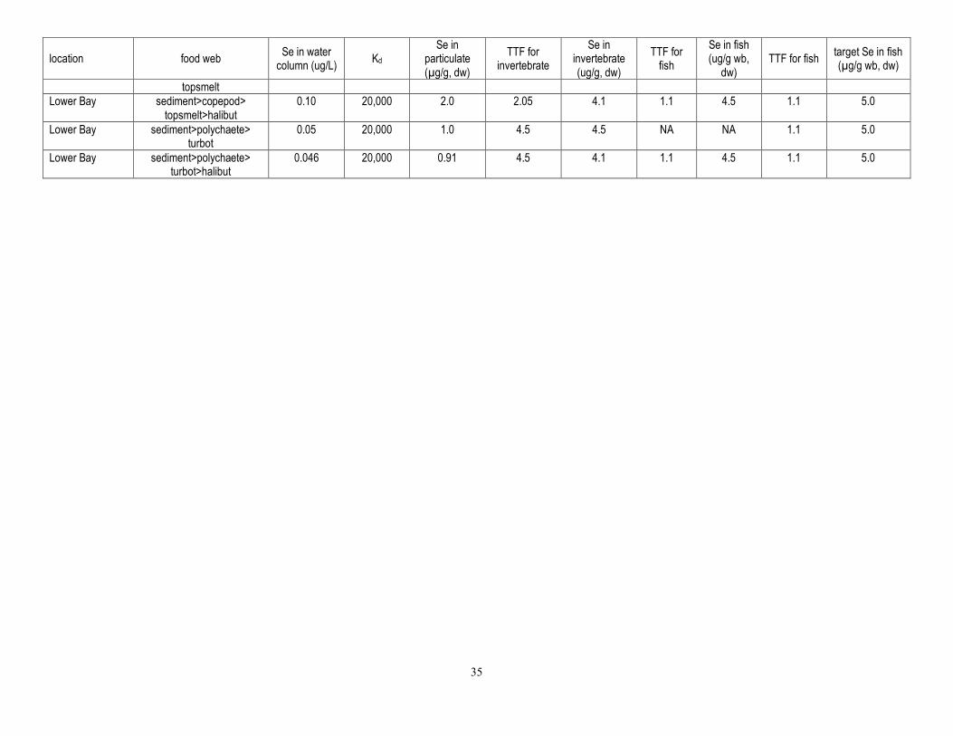
35





TTF for fish

Se in fish (ug/g wb,

dw) TTF for fish target Se in fish

(µg/g wb, dw)

topsmelt Lower Bay sediment>copepod>

topsmelt>halibut 0.10 20,000 2.0 2.05 4.1 1.1 4.5 1.1 5.0

Lower Bay sediment>polychaete> turbot

0.05 20,000 1.0 4.5 4.5 NA NA 1.1 5.0

Lower Bay sediment>polychaete> turbot>halibut

0.046 20,000 0.91 4.5 4.1 1.1 4.5 1.1 5.0

36

Table 21. Generalized modeled Se exposure scenarios for the watershed based on protection for fish. [dw = dry weight.] Se guideline for fish (µg/g dw) TTF for fish Se in invertebrate

(µg/g dw) TTF for aquatic insect Se in particulate (µg/g dw) Kd Se in water column

(ug/L)

Effect of varying Kd 5 1.1 4.55 2.8 1.62 136 (median) 11.94 5 1.1 4.55 2.8 1.62 168 (mean) 9.66 5 1.1 4.55 2.8 1.62 238 (75th percentile) 6.82 5 1.1 4.55 2.8 1.62 400 (wetland A) 4.06 5 1.1 4.55 2.8 1.62 800 (wetland B) 2.03 5 1.1 4.55 2.8 1.62 791 (UCI wetland mean) 2.05

Effect of varying fish guideline 8 1.1 7.27 2.8 2.60 136 (median) 19.10 7 1.1 6.36 2.8 2.27 136 (median) 16.71 6 1.1 5.45 2.8 1.95 136 (median) 14.32 5 1.1 4.55 2.8 1.62 136 (median) 11.94

Effect of varying fish guideline at a 75th percentile Kd 8 1.1 7.27 2.8 2.60 238 (75th percentile) 10.91 5 1.1 4.55 2.8 1.62 238 (75th percentile) 6.82

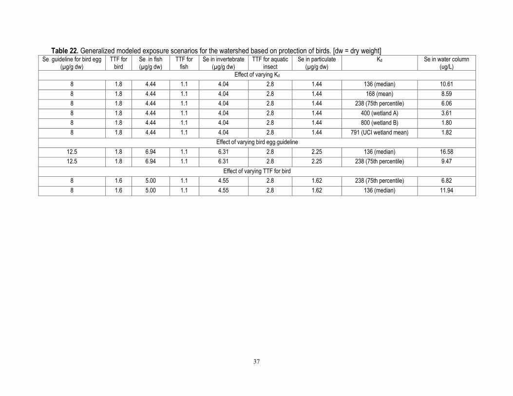
37

Table 22. Generalized modeled exposure scenarios for the watershed based on protection of birds. [dw = dry weight] Se guideline for bird egg

(µg/g dw) TTF for

bird Se in fish (µg/g dw)

TTF for fish

Se in invertebrate (µg/g dw)

TTF for aquatic insect

Se in particulate (µg/g dw)

Kd Se in water column (ug/L)

Effect of varying Kd 8 1.8 4.44 1.1 4.04 2.8 1.44 136 (median) 10.61 8 1.8 4.44 1.1 4.04 2.8 1.44 168 (mean) 8.59 8 1.8 4.44 1.1 4.04 2.8 1.44 238 (75th percentile) 6.06 8 1.8 4.44 1.1 4.04 2.8 1.44 400 (wetland A) 3.61 8 1.8 4.44 1.1 4.04 2.8 1.44 800 (wetland B) 1.80 8 1.8 4.44 1.1 4.04 2.8 1.44 791 (UCI wetland mean) 1.82

Effect of varying bird egg guideline 12.5 1.8 6.94 1.1 6.31 2.8 2.25 136 (median) 16.58 12.5 1.8 6.94 1.1 6.31 2.8 2.25 238 (75th percentile) 9.47

Effect of varying TTF for bird 8 1.6 5.00 1.1 4.55 2.8 1.62 238 (75th percentile) 6.82 8 1.6 5.00 1.1 4.55 2.8 1.62 136 (median) 11.94

38

Table 23. Model validation for Newport Bay showing predicted and observed fish Se concentrations. [SPM = suspended particulate material; max = maximum; dw = dry weight; n = number of samples.]

food web Se in

particulate (µg/g dw)


predicted Se in invertebrate (µg/g dw)

TTF for fish

predicted Se in fish

(µg/g, wb, dw)

observed Se in fish

(mean µg/g, wb, dw)

observed Se range in fish

(µg/g, wb, dw)

Upper Bay mean SPM>copepod>topsmelt 0.21 2.05 0.43 1.1 0.47 3.4 2.4-9.5 n=7 max SPM>copepod>topsmelt 1.00 2.05 2.05 1.1 2.26 mean SPM>polychaete>turbot 0.21 4.5 0.94 1.1 1.03 3.3 2.4-4.0 n=3 max SPM> polychaete>turbot 1.00 4.5 4.5 1.1 5.0 mean SPM>polychaete>killifish 0.21 4.5 0.94 1.1 1.03 5.8 2.6-9.5 n=5 max SPM> polychaete>killifish 1.00 4.5 4.5 1.1 5.0 mean SPM>clams>turbot 0.21 7.40 1.55 1.1 1.71 3.3 2.4-4.0 n=3 creekSPM>clams>turbot 1.00 7.40 7.40 1.1 8.14 meanSPM>anchovy>halibut 0.21 1.70 0.36 1.1 0.39 4.0 3.4-4.5 n=4 meanSPM>anchovy>halibut 1.00 1.70 1.70 1.1 1.87 sediments>mullet 2.00 2.0 4.00 5.5 2.4-9.5 n=7

Lower Bay sediments>amphipods>killifish 1.10 0.60 0.66 1.1 0.73 3.9 1.6-4.6 n=9 sediments>amphipods>killifish 2.98 0.60 1.79 1.1 1.97 sediment>copepod>topsmelt>halibut 1.10 2.05 and 1.1 2.50 1.1 2.75 1.5 0.9-3.1 n=4 sediment>copepod>topsmelt>halibut 2.98 2.05 and 1.1 6.70 1.1 7.40 1.5 sediment>polychaete>turbot 1.1 4.5 5.0 1.1 5.5 2.7 1.5-4.0 n=2 sediment>polychaete>turbot 2.98 4.5 13.4 1.1 14.7

39

Table 24. Model validation for bay showing (1) predicted and observed fish Se concentrations and (2) predicted and observed bird egg Se concentrations. [SPM = suspended particulate material; max = maximum; dw = dry weight; n = number of samples; NA = not available.]

food web Se in



predicted Se in

invertebrate (µg/g dw)

TTF for fish

predicted Se in fish

(µg/g, wb, dw)

observed Se in fish

(mean µg/g, wb, dw)

TTF for bird

predicted Se in bird egg, (µg/g dw)

observed Se in bird egg (µg/g

dw)a (skimmer/tern)

Se in bird egg from

observed fish ( µg/g dw)

Upper Bay mean SPM>copepod>topsmelt> skimmer, tern, grebe 0.21 2.05 0.43 1.1 0.47 3.4 1.8 0.85 3.1/4.4 6.1

max SPM 1.00 2.05 2.05 1.1 2.26 1.8 4.07 3.1/4.4 mean SPM>polychaete>turbot> skimmer, tern, grebe 0.21 4.5 0.94 1.1 1.03 3.3 1.8 1.85 3.1/4.4 5.9

max SPM 1.00 4.5 4.5 1.1 5.0 1.8 9.0 3.1/4.4 mean SPM>polychaete>killifish> skimmer, tern, grebe 0.21 4.5 0.94 1.1 1.03 5.8 1.8 1.85 3.1/4.4 10.4

max SPM 1.00 4.5 4.5 1.1 5.0 1.8 9.0 3.1/4.4 mean SPM>clams>turbot> skimmer, tern, grebe 0.21 7.40 1.55 1.1 1.71 3.3 1.8 3.1 3.1/4.4 5.9

max SPM>clams>turbot 1.00 7.40 7.40 1.1 8.14 1.8 14.6 3.1/4.4 mean SPM>anchovy>halibut> skimmer, ern, grebe 0.21 1.70 0.36 1.1 0.39 4.0 1.8 0.70 3.1/4.4 7.2

max SPM 1.00 1.70 1.70 1.1 1.87 1.8 3.4 3.1/4.4 mean sediment>mullet> skimmer, tern, grebe 2.00 2.0 4.00 5.5 1.8 7.2 3.1/4.4 9.9

Lower Bay sediment>amphipods>killifish> skimmer, tern, grebe 1.10 0.60 0.66 1.1 0.73 3.9 1.8 1.31 3.1/4.4 7.0

max sediment 2.98 0.60 1.79 1.1 1.97 1.8 3.54 3.1/4.4 sediment>copepod>topsmelt> halibut>pelican, osprey 1.10 2.05 and 1.1 2.50 1.1 2.75 1.5 1.8 4.95 3.1/4.4 2.7

max sediment 2.98 2.05 and 1.1 6.70 1.1 7.40 1.5 1.8 13.32 3.1/4.4 sediment>polychaete>turbot> skimmer, tern, grebe 1.1 4.5 5.0 1.1 5.5 2.7 1.8 9.9 3.1/4.4 4.9

max sediment 2.98 4.5 13.4 1.1 14.7 1.8 26.5 3.1/4.4 mean sediment>mullet>skimmer, tern, grebe 2.00 2.0 4.00 5.5 1.8 7.2 3.1/4.4 9.9

sediment 2.00 2.0 4.00 5.5 1.8 7.2 3.1/4.4 a ranges in bird egg Se concentrations (mean, range, and number of samples): skimmer, 3.1 µg/g dw (2.1-5.6) n=21; tern, 4.4 µg/g dw (2.5-8.4) n=18; and grebe, (from watershed) 6.1 µg/g dw (4-11) n=5

40

Table 25. Model validation for bay showing predicted and observed bird egg Se concentrations. [dw = dry weight; n = number of samples.]

food web particulate Se (µg/g dw)


predicted Se in

invertebrate (µg/g dw)

TTF for bird

predicted Se in bird

egg (µg/g, dw)

observed Se in bird

egga (µg/g, dw)

Se in bird egg (range, µg/g,

egg dw) number of samples

Upper Bay mean SPM>isopod>avocet 0.21 2.05 0.43 1.80 0.77 5.35 (1.6-10.7) n=12 creekSPM>isopod>avocet 1.00 2.05 2.05 1.80 3.69 5.35 mean SPM>isopod>rail 0.21 2.05 0.43 1.80 0.77 3.7 (3.1-4.5) n=6 creekSPM>isopod>rail 1.00 2.05 2.05 1.80 3.69 3.7 mean SPM>clams>scaup 0.21 7.40 1.55 1.80 2.80 NA creekSPM>clams>scaup 1.00 7.40 7.40 1.80 13.32 NA mean SPM>clams>rail 0.21 7.40 1.55 1.80 2.80 3.7 (3.1-4.5) n=6 creekSPM>clams>rail 1.00 7.40 7.40 1.80 13.32 3.7

Lower Bay sediment>clam>scaup 1.1 7.40 8.14 1.80 14.65 NA sediment>clam>scaup 2.98 7.40 22.05 1.80 39.69 NA sediment>clam>scaup 2 7.40 14.80 1.80 26.64 NA sediment>clam>scaup 2 7.40 14.80 1.80 26.64 NA a additional bird egg Se concentrations (mean, range, and number of samples): stilt, 5.1 µg/g dw (3.4-8.5 ) (n=3); and killdeer, 2.6 µg/g dw (2.3-2.9) (n=2)

41

Table 26. Model validation for watershed showing (1) predicted and observed invertebrate Se concentrations and (2) predicted and observed bird egg Se concentrations. [dw = dry weight; n = number of samples]

location food web invertebrate Se in



predicted Se in invertebrate (µg/g dw)

observed in invertebrate (average)

TTF for bird


egg (µg/g, dw)

observed Se in bird egg (µg/g, dw)

species and number of samples

Lower SDC sediment>invertebrate> avocet

corixid, crayfish, snail, clam

1.2 2.8

2.8 2.8

3.4 7.8

6.2 1.8 1.8

6.2 14.0

2.8 (1.9-3.9)

avocet (3)

Lower SDC sediment>invertebrate> stilt


2.8 1.8 6.9 (3.6-8.7)

stilt (11)

Lower SDC sediment>invertebrate> killdeer


2.8 1.8 9.5 (9.1-9.9)

killdeer (2)

Lower SDC sediment>invertebrate> grebe


2.8 1.8 5.8 pied-billed grebe (1)

Lower SDC sediment>invertebrate> coot


2.8 1.8 5.2 coot (1)

IRWD wetlands sediment>invertebrate> avocet

midge, corixid, dragonfly

3.7 5.3

2.8 10.4 14.8

10.9

1.8 18.7 26.6

6.4 (2-17.2)

avocet (8)

IRWD wetlands sediment> invertebrate> stilt

zooplankton, midge, corixid, snail, crayfish,

dragonfly, clam

2.8 1.8 5 (3-9.8)

stilt (4)

IRWD wetlands sediment> invertebrate> mallard


dragonfly, clam

2.8 1.8 6.2 (4-7)

mallard (4)

IRWD wetlands sediment> invertebrate> killdeer


dragonfly, clam

2.8 1.8 4.8 (2.6-7.1)

killdeer (2)

UCI wetlands sediment> invertebrate> coot

dragonfly 2.2 2.8 6.2 5.6 1.8 11.2 2.7 (1.9-4.5)

coot (9)

UCI wetlands sediment> invertebrate> avocet

dragonfly 2.8 1.8 5.1 (3.3-11)

avocet (5)

UCI wetlands sediment> invertebrate> grebe

dragonfly 2.8 1.8 6.2 (4-11)

pied-billed grebe (4)

42

Table 27. Model validation for watershed showing (1) predicted and observed fish Se concentrations and (2) predicted and observed bird egg Se concentrations. [dw = dry weight; n = number of samples.]

location food web fish species

particulate Se (µg/g dw)


predicted Se in inverte-brate

(µg/g dw) TTF for

fish predicted Se in fish (µg/g dw)

average observed

in fisha TTF for

bird


egg (µg/g, dw)

observed Se in bird

egg (µg/g, dw)

species and

number of samples

Lower San Diego Creek

sediment> invert>fish>bird

average fish

1.2 2.8

2.8 3.4 7.8

1.1 1.1

3.7 8.6

8.4


IRWD wetlands sediment> invert>fish>bird

average fish

3.7 5.3

2.8 10.4 14.8

1.1 1.1

11.4 16.3

14 1.8 25.2

UCI wetlands sediment> invert> grebe

average fish

2.2 2.8 6.2 1.1 6.8 5.8 1.8 10.4 6.2 (4-11)

pied-billed grebe (4)

a mosquitofish for marsh drains, lower San Diego Creek, and Lower Peters Canyon Wash were 12.5, 17 and 21 µg/g dw, respectively; thus, transfer for mosquitofish at these sites are underestimated by a TTF of 1.1 (see table 11 for range of TTFs for mosquitofish)

43

Table 28. Model validation for watershed showing predicted and observed bird egg Se concentrations. [dw = dry weight; n = number of samples.]

location food web Se in fish (µg/g, wb, dw) fish species TTF for

bird predicted Se in bird

egg (µg/g, dw) observed Se in

bird egg (µg/g, dw)

species and number of bird egg samples

Upper SDC and PCW sediment>invert>fish>bird 5.8 mixed fish 1.8 10.4 Marsh drains sediment>invert>fish>bird 12.5 mosquitofish 1.8 22.5 Lower SDC sediment>invert>fish>bird 7.8 bluegill, common carp, fathead

minnow, red shiner, largemouth bass, black crappie, white catfish, mixed fish


Lower SDC sediment>invert>fish>bird 17 mosquitofish 1.8 30.6 Lower PCW sediment>invert>fish>bird 6.4 fathead minnow, red shiner 1.8 11.5 Lower PCW sediment>invert>fish>bird 21 mosquitofish (12.1; 29.9) 1.8 37.8 IRWD wetlands sediment>invert>fish>bird 19.3 dead carp (filet) 1.8 34.7 IRWD wetlands sediment>invert>fish>bird 13 mixed fish 1.8 23.4 IRWD wetlands sediment>invert>fish>bird 10.1 mosquitofish (2.3; 15.3) 1.8 18.2 UCI wetlands sediment>invert>fish>bird 5.8 mosquitofish 1.8 10.4 6.2 (4.0-11) pied-billed

grebe (4)

44

Figures Figure 1. Schematic block diagram of the San Diego Creek watershed and Newport Bay highlighting assessment areas and Se pathway. Map enlargement shows Upper and Lower Newport Bay.

45

Figure 2. Conceptual model for the San Diego Creek watershed illustrating linked factors that determine the effects of Se on ecosystems.

46

Figure 3. Conceptual model for the Upper Newport Bay illustrating linked factors that determine the effects of Se on ecosystems.

47

Figure 4. Conceptual model for the Lower Newport Bay illustrating linked factors that determine the effects of Se on ecosystems.

48

Figure 5. Extrapolation of dissolved Se to 0 ppt. Data from transect of the Upper Newport Bay from near the mouth of San Diego Creek into the upper bay (CH2M Hill, 2008a).

0

5

10

15

20

25

0 5 10 15 20 25 30 35

Dis

solv

ed S

e, m

icro

gram

s pe

r lite

r (µg

/L)

Salinity, parts per thousand (ppt)

y = 24.53 - 0.74507x

R2 = 0.96067

Documents

Modeling of Selenium for the San Diego Creek Watershed and ... › of › 2009 › 1114 › of2009-1114.pdf · The San Diego Creek watershed and Newport Bay in southern California