MODELING OF REYNOLDS-STRESS AUGMENTATION IN …congress.cimne.com/iacm-eccomas2014/admin/files/filePaper/p1349.pdfround turbulent jet, which exhibits an overestimated jet core length

11th World Congress on Computational Mechanics (WCCM XI)5th European Conference on Computational Mechanics (ECCM V)

6th European Conference on Computational Fluid Dynamics (ECFD VI)E. Onate, J. Oliver and A. Huerta (Eds)

MODELING OF REYNOLDS-STRESS AUGMENTATION INSHEAR LAYERS WITH STRONGLY CURVED VELOCITY

PROFILES

RENE-DANIEL CECORA∗, ROLF RADESPIEL∗ AND SUAD JAKIRLIC†

∗ Institute of Fluid MechanicsTechnische Universitat Braunschweig

Hermann-Blenk-Str. 37, 38108 Braunschweig, Germanye-mail: [email protected], web page: www.tu-braunschweig.de/ism

† Institute of Fluid Mechanics and AerodynamicsTechnische Universitat Darmstadt

Alarich-Weiss-Str. 10, 64287 Darmstadt, Germanyweb page: http://www.sla.tu-darmstadt.de/sla

Key words: RANS, Reynolds-stress turbulence modeling, free shear flows

Abstract. An extension and re-calibration of a differential Reynolds-stress model isperformed, which is influential in shear layers where the velocity profile shows large secondderivatives. Besides a backward-facing step flow and a zero-pressure-gradient flat plate,which are used for calibration, further test cases are simulated with the new model forvalidation purposes. Especially the simulation of the flow over a transonic bump canbe improved with the new model version JHh-v3, further improvements are made for aturbulent round jet.

1 INTRODUCTION

Numerical flow simulation is an important tool in the development process of aircraftindustry. Solving of the Reynolds-Averaged Navier-Stokes (RANS) equations is regardedas a good compromise between computational effort and accuracy. The quality of RANSsimulations highly depends on the modeling of the Reynolds-stress tensor as a measurefor the statistical influence of turbulence on the mean flow.

The most commonly used turbulence models in an industrial environment are so-callededdy-viscosity models (e.g. [1, 2]), which link the Reynolds stresses to the shear rate of themean flow via an eddy viscosity as a proportionality factor. Mostly one or two transportequations are solved to provide the eddy viscosity. Second-moment closure (SMC) models,on the other hand, directly employ transport equations for the Reynolds stresses, offering

1

Rene-Daniel Cecora, Rolf Radespiel and Suad Jakirlic

a higher potential for an adequate predicition of complex flows. They are often refered toas Reynolds-stress models (RSM).

Recently Cecora et al. [3] presented a SMC model (JHh-v2) which showed promis-ing results in different aeronautical applications, containing high-lift airfoil flow andshock/boundary-layer interaction. It was however noticed that the JHh-v2 model un-derestimates the development of turbulence in shear layers with inflection point in thevelocity profile. Corresponding examples are the backward-facing step (BFS) flow, inwhich the slowly developing turbulence causes too long separation length, as well as theround turbulent jet, which exhibits an overestimated jet core length. A remedy is foundby implementing an additional sink term, which is sensitized towards shear flows withinflection point, into the length-scale equation. The successful application of this termto a similar Reynolds-stress model (RSM-PSAS) has already been shown by Maduta [4]and Jakirlic and Maduta [5]. The two RSM are both evolved from the JH model [6], theymainly differ in the length-scale equation, with the JHh-v2 employing the homogeneousdissipation rate εh as length-scale variable while the RSM-PSAS model uses the homoge-neous part of the inverse time scale ωh = εh/k. Furthermore the JHh-v2 model containsan additional source term in the length-scale equation which sensitizes the model towardsadverse pressure gradients. Last but not least the models use a different set of coefficientsin the length-scale equation.

In this paper, the extension and calibration of the JHh-v2 model is presented, usinga backward-facing step flow and a zero-pressure-gradient flat plate flow as calibrationcases. The resulting model is named as JHh-v3. The performance of the JHh-v3 model isvalidated considering two wall-bounded transonic flows as well as a turbulent round jet.

2 NUMERICAL METHOD

The following investigations have been carried out using the DLR-TAU Code [7], afinite-volume solver which solves the Favre- and Reynolds-averaged Navier-Stokes equa-tions on hybrid unstructured grids with second order accuracy.

Closure of the equation system is achieved with a differential Reynolds-stress turbulencemodel. It is based on a near-wall RSM by Jakirlic and Hanjalic [6] (JH RSM), which wasimplemented into the DLR-TAU Code by Probst and Radespiel [8]. A re-calibration fordifferent aeronautical test cases was conducted by Cecora et al. [3], resulting in the modelversion JHh-v2, which is further developed in this work.

2.1 Extension of the JHh-v2 Model for Free Shear Flows

It was noted that the current version of the Reynolds-stress model (JHh-v2) tendsto underestimate the growth of Reynolds stresses in free shear layers which contain aninflection point in the velocity distribution. As a remedy, an additional sink term is im-plemented into the length-scale equation with the intention of locally reducing dissipationand hence supporting the development of turbulence. After implementation, the RSM is

2


re-calibrated and named as JHh-v3.The background of the implemented sink term can be found within the k − kL model

of Rotta [9], which employs a transport equation for the quantity kL, with L being anintegral length scale of turbulence:

kL =3

16

∞∫

−∞

Rii (~x, ry) dry . (1)

Rij describes the two-point correlation tensor of the velocity fluctuation u′i, considering the

Einstein summation convention for Rii. In the derivation of the modeled kL equation froman exact transport equation, Rotta notices a second production term that is influentialon the performance of his turbulence model. Menter and Egorov [10] proposed theirown way of modeling this term, furthermore they transformed it to different length-scalevariables in order to make it suitable for modern turbulence models [10, 11]. This secondproduction term contains second derivatives of the velocity tensor, which enables theturbulence model to account for additional length scales within the mean velocity field.Combining it with an eddy-viscosity model gave birth to the so-called Scale AdaptiveSimulation (SAS) concept [10], in which the turbulence model is sensitized for resolvinginstabilities by locally reducing modeled turbulence. The additional source term especiallycontributes in shear flows with velocity distributions containing inflection points, which isan indicator for a tendency towards instability. Combined with the length-scale equationof modern eddy-viscosity models, the source term reduces the modeled turbulence in theaffected region, causing the simulation to develop unsteadiness. Using these turbulencemodels with SAS-extension in a time-accurate flow solver (URANS) allows for an improvedprediction of turbulence in shear layers with a tendency towards instability. Instead ofcombining the additional source term to an eddy-viscosity model, Maduta and Jakirlic[12] use the SAS concept in combination with a second-moment closure model.

While the SAS concept is intended to resolve a wide part of the turbulent spectrum inunsteady flow regions, the opposite approach followed in this work is to consider a widerspectrum of instabilities within the turbulence model. Therefore the SAS source term isused as a sink term in the length-scale equation of the Reynolds-stress model:

Dεh(JHh−v3)

Dt=

Dεh(JHh−v2)

Dt− PSAS . (2)

This idea was proposed and successfully applied by Maduta [4] using the JH Reynolds-stress model in combination with a ωh length-scale equation. After transformation ofMaduta’s term into an εh formulation, the implemented sink term reads:

PSAS = CSAS,1max [PSAS,1 − PSAS,2, 0] , (3)

with

PSAS,1 = 1.755κkS2

(

L

Lvk

)1

2

(4)

3


and

PSAS,2 = 3k2max

(

CSAS,2(∇εh)2k2 + (∇k)2(εh)2 − 2kεh∇εh∇k

k2(εh)2,(∇k)2

k2

)

. (5)

The formulation contains the turbulent length scale L = k3/2/εh and the 3D generalizationof the classical boundary-layer definition of the von Karman length scale Lvk = κS/ |∇2U |.

3 CALIBRATION OF THE ADDITIONAL SINK TERM

Although the model investigated in this work is derived from the same Reynolds-stressmodel as the one shown by Maduta [4] and as Maduta and Jakirlic [5], minor differencescan be found in the formulations and in the model coefficients. Therefore the sink termcan not be just transformed from ωh to εh, it has to be calibrated as well. The additionalsink term (Eq. (3)-(5)) contains two coefficients that need to be calibrated: CSAS,1 andCSAS,2, where the former is responsible for the global impact of the term compared to theregular source terms. The latter modifies the term itself.

In Fig. 1, the distribution of the ratio of PSAS,1 and the main destruction term Yεh1 is

shown for the backward-facing step flow, simulated with the basic JHh-v2 RSM. A strongcontribution can be seen in the developing shear layer between the recirculating flow andthe outer flow. Furthermore significant values are found in the boundary layer upstreamof the step, very close to the wall.

x / H

z/H

-4 -2 0 2 4 6 8 10 12 140

2

410987654321

PSAS,1/Yεh

Figure 1: BFS. Ratio of PSAS,1 to main destruction term Yεh .

Corresponding profiles of PSAS,1 at two different streamwise positions, upstream of the

1Due to the modeling formulation of a combined production-destruction, i.e. derived from two termsin the exact ε equation, the sink term is originally refered to as P 4

ε − Y [13]. As a simplification andin order to illustrate its function as destruction term of the εh equation, the sink term is in this workdenoted as Yεh .

4


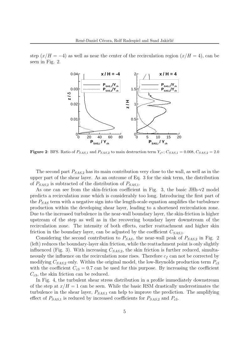
step (x/H = −4) as well as near the center of the recirculation region (x/H = 4), can beseen in Fig. 2.

PSAS,i / Yεh

z/δ

0 20 40 60 800

0.01

0.02

0.03

0.04

PSAS,1/Yεh

PSAS,2/Yεh

x / H = -4

PSAS,i / Yεh

z/H

0 5 10 15 200

0.5

1

1.5

2

PSAS,1/Yεh

PSAS,2/Yεh

x / H = 4

Figure 2: BFS. Ratio of PSAS,1 and PSAS,2 to main destruction term Yεh ; CSAS,1 = 0.008, CSAS,2 = 2.0

The second part PSAS,2 has its main contribution very close to the wall, as well as in theupper part of the shear layer. As an outcome of Eq. 3 for the sink term, the distributionof PSAS,2 is subtracted of the distribution of PSAS,1.

As one can see from the skin-friction coefficient in Fig. 3, the basic JHh-v2 modelpredicts a recirculation zone which is considerably too long. Introducing the first part ofthe PSAS term with a negative sign into the length-scale equation amplifies the turbulenceproduction within the developing shear layer, leading to a shortened recirculation zone.Due to the increased turbulence in the near-wall boundary layer, the skin-friction is higherupstream of the step as well as in the recovering boundary layer downstream of therecirculation zone. The intensity of both effects, earlier reattachment and higher skinfriction in the boundary layer, can be adjusted by the coefficient CSAS,1.

Considering the second contribution to PSAS, the near-wall peak of PSAS,2 in Fig. 2(left) reduces the boundary-layer skin friction, while the reattachment point is only slightlyinfluenced (Fig. 3). With increasing CSAS,2, the skin friction is further reduced, simulta-neously the influence on the recirculation zone rises. Therefore cf can not be corrected bymodifying CSAS,2 only. Within the original model, the low-Reynolds production term Pε3

with the coefficient Cε3 = 0.7 can be used for this purpose. By increasing the coefficientCε3, the skin friction can be reduced.

In Fig. 4, the turbulent shear stress distribution in a profile immediately downstreamof the step at x/H = 1 can be seen. While the basic RSM drastically underestimates theturbulence in the shear layer, PSAS,1 can help to improve the prediction. The amplifyingeffect of PSAS,1 is reduced by increased coefficients for PSAS,2 and Pε3.

5


x / H

c f

0 10 20

0

0.002

0.004

Driver 1985JHh-v2CSAS1=8e-3CSAS1=8e-3, CSAS2=2CSAS1=8e-3, Cε3=1.8JHh-v3

Figure 3: BFS. Skin-friction coefficient alongthe wall.

1000*u’w’/U ∞2

z/H

-10 -5 00

0.5

1

1.5

2 Exp., x/H=1JHh-v2CSAS1=-8e-3CSAS1=-8e-3, CSAS2=2CSAS1=-8e-3, Cε3=1.8JHh-v3

Figure 4: BFS. Profile of turbulent shear stressat streamwise position x/H = 1.

For a precise adjustment of the skin friction in boundary layers, a zero-pressure-gradient(ZPG) flat plate has to be simulated. As we have already seen in the backward-facingstep flow, the skin friction rises when PSAS,1 is activated (Fig. 5).

Rex

c f

0 5E+06 1E+070

0.002

0.004

0.006 Exp.JHh-v2CSAS,1=0.008JHh-v3

Figure 5: Zero-Pressure-Gradient Flat Plate. Skin-friction coefficient along the wall.

Agreeable results for both calibration cases, backward-facing step as well as ZPG flatplate, are achieved for the following coefficient set: CSAS,1 = 0.008, CSAS,2 = 2.0, Cε3 =1.8. The resulting model is named as JHh-v3. When the shear-stress profile in Fig. 4 isconsidered, even higher values of CSAS,1 seem appropriate to obtain agreeable turbulence

6


levels. The coefficients found here are however regarded as a reasonable compromise ofthe cases investigated so far.

4 VALIDATION OF THE EXTENDED MODEL

Since the model formulation and its coefficients are changed, the new turbulence modelversion has to be validated against different test cases, in order to evaluate its performancefor a wide range of aeronautical flows.

4.1 Round Single-Stream Jet

Similar to the backward-facing step flow, a shear layer with inflection point developsbetween a jet and the stagnant or slowly moving ambiance. The turbulent M = 0.75 jetthat emerges from a round nozzle was simulated on a hexahedral mesh with 9 ·106 points.Velocity profiles as well as profiles of the turbulent shear stress component u′v′ can beseen in Fig. 6, in comparison to experimental results [14].

U/U j

y/D

0 0.5 10

0.4

0.8

1.2 ExperimentJHh-v2JHh-v3

x / D = 1

U/U j

y/D

0 0.5 10

0.4

0.8

1.2

x / D = 5

R12/U j2

y/D

0 0.01 0.020

0.4

0.8

1.2

x / D = 1

R12/U j2

y/D

0 0.01 0.020

0.4

0.8

1.2

x / D = 5

Figure 6: Round Single-Stream Jet. Profiles of velocity (upper line) and turbulent shear stress (lowerline), at two streamwise positions.

7


Already early in the developing shear layer (x/D = 1, with x having its origin at thenozzle exit), the JHh-v2 model underestimates the turbulent shear stress, similarly to theBFS flow. The lack of turbulence is still existent at x/D = 5, showing furthermore aninfluence on the velocity profile. An improvement is found in the simulation with theJHh-v3 model, where higher levels of turbulence increase the transport of momentum,giving a velocity profile with a better agreement to the experimental data. Neverthelessthe peak values of u′v′ are underpredicted.

The underestimated transport of momentum has a lengthening effect on the jet core,which can be seen in Fig. 7. The velocity on the jet axis is shown for both RSM versions

x/D

U/U

j

0 5 10 150

0.2

0.4

0.6

0.8

1

1.2

ExperimentsJHh-v2JHh-v3

Figure 7: Round Single-Stream Jet. Axial velocity ratio along the jet axis.

as well as for the experiments, with Uj being the axial velocity at x/D = 0. Whilein experiments the axial velocity starts to decrease at xc/D = 5...6, JHh-v3 predictsxc/D ≈ 8.8 and JHh-v2 even xc/D ≈ 10.4.

4.2 Transonic Airfoil RAE 2822

The supercritical flow around the RAE 2822 airfoil is a standard test case for turbulencemodels, experimental data is provided by Cook et al. [15]. Fig. 8 shows a comparison ofmeasured and simulated pressure distribution at Mach number M = 0.73 and Reynoldsnumber Re = 6.5 · 106, also known as Case 9. It can be seen that the influence of theadditional sink term in combination with the re-calibration is rather small for this fullyattached airfoil flow. A small contribution can be found in the decelerated boundary layernear the shock, increasing the turbulence and therefore stabilizing the boundary layer.As a result, the shock moves slightly downstream.

8


4.3 Transonic Axisymmetric Bump

The flow at transonic Mach number over an axisymmetric bump is a complex test casefor turbulence models. It develops a compression shock which interacts with the boundarylayer and induces a flow separation over the rear part of the bump, before it reattachesfurther downstream. Experiments have been conducted by Bachalo and Johnson [16, 17].The axisymmetric problem was simulated on a 2D grid of 48000 points that was rotated by5◦, employing an axisymmetry boundary condition on both sides. The 2D grid contains300 points in streamwise direction, of which 150 discretize the bump geometry. Theboundary layer upstream of the bump is resolved by 90 points in wall-normal direction.

In order to adequately predict the shock location as well as the separation point, agood quality of the turbulence model in simulating the upstream boundary layer throughfavorable and adverse pressure gradient is essential. The reattachment point howeverstrongly depends on the turbulent shear stresses that develop in the separated shearlayer.

Fig. 9 shows a comparison of the simulated pressure distribution with experiments.It can be noticed that the basic JHh-v2 model overestimates the size of the separation,

x/c

Cp

0 0.2 0.4 0.6 0.8 1

-1

-0.5

0

0.5

1

ExperimentJHh-v2JHh-v3

Figure 8: Transonic Airfoil RAE 2822, Case 9.pressure coefficient along the airfoil.

x/c

c p

0.6 0.8 1 1.2 1.4

-0.8

-0.6

-0.4

-0.2

0

0.2

Ma 0.875SAOMenter SSTJHh-v2JHh-v3

Figure 9: Transonic Axisymmetric Bump. Pres-sure coefficient along the wall.

which results in an exaggerated pressure plateau around x/c = 1. Furthermore the shockposition is found slightly upstream of the experimental prediction. Clear improvementsof the pressure distribution can be found when using the JHh-v3 model, especially inthe recovering boundary layer downstream of the separation (x/c ≈ 1.2). The pressureplateau is even underestimated, while the shock position shows a good agreement to the

9


experimental data. A comparison of shock position, separation location and reattachmentlocation is given in Tab. 1.

Table 1: Transonic Axisymmetric Bump. Comparison of simulated and measured flow topology.

SAO Menter SST JHh-v2 JHh-v3 Exp.

Shock position2 0.690 0.645 0.633 0.653 0.66Separation point 0.690 0.645 0.667 0.689 0.70

Reattachment point 1.165 1.174 1.194 1.092 1.10Length of separation 0.475 0.529 0.527 0.403 0.40

Distance of separation to shock 0.000 0.000 0.034 0.036 0.04

It can be noticed that the prediction of the reattachment point and thus the length ofthe separation is improved in the simulation with JHh-v3. Furthermore the shock movesslightly downstream, similar to the RAE 2822 case. While both eddy-viscosity modelsshow an immediate separation at the shock, the boundary layer endures the adversepressure gradient for a short distance in the simulations with both RSM versions, whichagrees to the experimental data.

5 CONCLUSION

The extension of the length-scale equation of a differential Reynolds-stress turbulencemodel with an additional sink term has been presented. It was shown that the modificationamplifies the development of turbulence in free shear flows, which positively influencesthe separation length of a backward-facing step flow. Furthermore the overprediction ofthe core length in turbulent round jets is reduced. Only minor influence is noticed inthe simulation of the attached flow around the transonic airfoil RAE 2822, whereas theprediction of the separated flow over a transonic bump is improved.

Acknowledgments

The authors gratefully acknowledge the “Bundesministerium fur Bildung und Forschung”who funded parts of this research within the frame of the joint project AeroStruct (fund-ing number 20 A 11 02 E), as well as the “North-German Supercomputing Alliance” forsupplying us with computational resources within the project nii00090. Furthermore wewould like to thank A. Probst of DLR Gottingen who provided a computational meshand his experience for the BFS flow.

2In the simulations, the shock position is not a discrete point. The measured shock position corre-sponds to a pressure coefficient of cp = −0.49, which was used for determination of the simulated shockpositions.

10


REFERENCES

[1] Spalart, P. R., Allmaras, S. R. A one-equation turbulence model for aerodynamicflows. La Recherche Aerospatiale (1994) 1:5–21.

[2] Menter, F. R. Two-Equation Eddy-Viscosity Turbulence Models for Engineering Ap-plications. AIAA Journal (1994) 32(8):1598–1605.

[3] Cecora, R.-D., Eisfeld, B., Probst, A., Crippa, S. and Radespiel, R. DifferentialReynolds Stress Modeling for Aeronautics. 50th AIAA Aerospace Sciences Meeting

(2012) Nashville, Jan. 9-12.

[4] Maduta, R. An eddy-resolving Reynolds stress model for unsteady flow computations:development and application. Dissertation, TU Darmstadt (2014).

[5] Jakirlic, S. and Maduta, R. On “Steady” RANS Modeling for improved Prediction ofWall-bounded Separation. 52nd AIAA Aerospace Sciences Meeting (2014) NationalHarbor, MD, USA.

[6] Jakirlic, S. and Hanjalic, K. A new approach to modelling near-wall turbulence energyand stress dissipation. Journal of Fluid Mechanics (2002) 459:139–166.

[7] Schwamborn, D., Gardner, A., von Geyr, H., Krumbein, A., Ludeke, H. and Sturmer,A. Development of the TAU- Code for aerospace applications. 50th NAL International

Conference on Aerospace Science and Technology (2008) Bangalore, India.

[8] Probst, A. and Radespiel, R. Implementation and Extension of a Near-Wall Reynolds-Stress Model for Application to Aerodynamic Flows on Unstructured Meshes. 46thAIAA Aerospace Sciences Meeting and Exhibit (2008).

[9] Rotta, J. C. Turbulente Stromungen. Stuttgart: B. G. Teubner (1972).

[10] Menter, F. R., and Egorov, Y. A Scale-Adaptive Simulation Model using Two-Equation Models. AIAA-Paper 2005-1095 (2005).

[11] Menter, F. R., and Egorov, Y. The Scale-Adaptive Simulation Method for UnsteadyTurbulent Flow Predictions. Part 1: Theory and Model Description. Flow, Turbulenceand Combustion (2010) 85(1):113-138.

[12] Maduta, R., and Jakirlic, S. An eddy-resolving Reynolds stress transport model forunsteady flow computations. In: Advances in Hybrid RANS-LES Modelling 4. Noteson Numerical Fluid Mechanics and Multidisciplinary Design. (2012) 117: 77-89.

[13] Jakirlic, S. A DNS-Based Scrutiny of RANS Approaches and Their Potential forPredicting Turbulent Flows. Habilitationsschrift, TU Darmstadt (2004).

11


[14] Jordan, P., Gervais, Y., Valiere, J.-C. and Foulon, H. Final results from single pointmeasurements. Project deliverable D3.4, JEAN - EU 5th Framework Programme,

G4RD-CT2000-00313 (2002) Laboratoire dEtude Aerodynamiques, Poitiers.

[15] Cook, P. H., McDonald, M. A., Firmin, M. C. P. Aerofoil RAE 2822 – PressureDistributions, and Boundary Layer and Wake Measurements. In: J. Barche (Ed.),Experimental Data Base for Computer Program Assessment (1979) AGARD-AR-138A6.

[16] Bachalo, W. D., and Johnson, D. A. An Investigation of Transonic Turbulent Bound-ary Layer Separation Generated on an Axisymmetric Flow Model. AIAA 12th Fluid

and Plasma Dynamics Conference (1979) Williamsburg, Virginia.

[17] Bachalo, W. D., and Johnson, D. A. Transonic, Turbulent Boundary-Layer Separa-tion Generated on an Axisymmetric Flow Model. AIAA Journal (1986) 24(3):437-443.

12

Documents

MODELING OF REYNOLDS-STRESS AUGMENTATION IN …congress.cimne.com/iacm-eccomas2014/admin/files/filePaper/p1349.pdfround turbulent jet, which exhibits an overestimated jet core length