micromachines

Article

Modeling of Knudsen Layer Effects in theMicro-Scale Backward-Facing Step in the SlipFlow Regime

Apurva Bhagat , Harshal Gijare and Nishanth Dongari ∗

Department of Mechanical and Aerospace Engineering, Indian Institute of Technology, Hyderabad, Kandi,Medak 502285, India; me13m15p000001@iith.ac.in (A.B.); me13m15p000002@iith.ac.in (H.G.)* Correspondence: nishanth@iith.ac.in

Received: 27 December 2018; Accepted: 2 February 2019; Published: 12 February 2019�����������������

Abstract: The effect of the Knudsen layer in the thermal micro-scale gas flows has been investigated.The effective mean free path model has been implemented in the open source computationalfluid dynamics (CFD) code, to extend its applicability up to slip and early transition flow regime.The conventional Navier-Stokes constitutive relations and the first-order non-equilibrium boundaryconditions are modified based on the effective mean free path, which depends on the distance fromthe solid surface. The predictive capability of the standard ‘Maxwell velocity slip—Smoluchwoskitemperature jump’ and hybrid boundary conditions ‘Langmuir Maxwell velocity slip—LangmuirSmoluchwoski temperature jump’ in conjunction with the Knudsen layer formulation has beenevaluated in the present work. Simulations are carried out over a nano-/micro-scale backward facingstep geometry in which flow experiences adverse pressure gradient, separation and re-attachment.Results are validated against the direct simulation Monte Carlo (DSMC) data, and have shownsignificant improvement over the existing CFD solvers. Non-equilibrium effects on the velocityand temperature of gas on the surface of the backward facing step channel are studied by varyingthe flow Knudsen number, inlet flow temperature, and wall temperature. Results show that themodified solver with hybrid Langmuir based boundary conditions gives the best predictions whenthe Knudsen layer is incorporated, and the standard Maxwell-Smoluchowski can accurately capturemomentum and the thermal Knudsen layer when the temperature of the wall is higher than thefluid flow.

Keywords: rarefied gas flows; micro-scale flows; Knudsen layer; computational fluid dynamics(CFD); OpenFOAM; Micro-Electro-Mechanical Systems (MEMS); Nano-Electro-Mechanical Systems(NEMS); backward facing step

1. Introduction

Conventional Navier-Stokes (NS) equations are based on the assumption that the mean free path(MFP) of the particle is much smaller than the characteristic length scale of the system. However, in afew engineering applications of interest, this continuum assumption deviates, if the flow is highlyrarefied (e.g., vehicles operating at high altitude conditions), or length scale of the system is of theorder of MFP of the gas (e.g., micro-scale gas flows). Flow through the nano-/micro-scale devicesis dominated by non-equilibrium effects such as rarefaction and gas molecule-surface interactions.Knudsen layer (KL) is one such phenomenon, where a non-equilibrium region is formed near the solidsurface in rarefied/micro-scale gas flows. Molecule-surface collisions are dominated by the presence ofa solid surface reducing the mean time between collisions, i.e., unconfined MFP of the gas is effectivelyreduced in the presence of a solid surface [1]. Molecules collide with the wall more frequently than

Micromachines 2019, 10, 118; doi:10.3390/mi10020118 www.mdpi.com/journal/micromachines

Micromachines 2019, 10, 118 2 of 15

with other molecules, leading to the formation of the Knudsen layer as demonstrated in Figure 1.Linear constitutive relations for shear stress and heat flux are no longer valid in this region [2–4].

Figure 1. Schematic of inter-molecular and molecule-surface collisions leading to the formation ofKnudsen layer (KL).

Behavior of the non-equilibrium gas flows and structure of KL have been extensively investigatedby directly solving the Boltzmann equation [5], kinetic equations (e.g., the BGK (Bhatnagar, Gross andKrook) model, rigid-sphere model, the Williams model) [6–9] or alternative hydrodynamic models suchas the Burnett equation, super-Burnett equations, Grad 13 moment equation and the regularized Gradmoment equations [2,10–13]. However, obtaining solutions using these models is computationallychallenging due to the complicated structure of molecular collisions term, lack of well-posed boundaryconditions and inherent instability. The direct simulation Monte Carlo (DSMC) technique [14,15] isone of the most accepted and reliable methods for solving gas flows in the non-equilibrium region.Collisions of some representative particles with each other and wall boundaries, are handled in astochastic manner [16]. As a result, computational cost becomes pretty intensive in case of micro-scaleflows due to high density and low flow velocity. A few researchers [17–19] have applied DSMC methodto analyze gas flow through micro-channel, and statistical scatter have been a critical issue. A hugesample size is required to reduce the statistical scatter, which makes the DSMC simulation tedious andtime-consuming. These difficulties can be overcome if NS equations are extended with higher-orderconstitutive relations and boundary conditions so that they can accurately capture the Knudsen layerand non-linear flow physics of micro-scale gas flows.

Few researchers have attempted to include non-equilibrium effects in NS framework fromdifferent viewpoints. Myong [13] has derived the second-order macroscopic constitutive equationfrom the kinetic Boltzmann equation and obtained analytical solutions to the KL in Couette flowwithin continuum frame-work. Li et al. [20] have proposed an effective viscosity model to accountfor the wall effect in the wall adjacent layer. Lockerby et al. [21] have introduced the concept ofwall function into a scaled stress-strain rate relation by fitting the velocity profile obtained fromthe linearized Boltzmann equation. This idea has been further extended to obtain Kn dependentfunctions [22], power-law scaling of constitutive relations [23] and discontinues correction functionfor near wall and far wall region [24,25]. The key disadvantage of these models is that they usuallycontain some empirical parameters which are specific for the geometry and the flow conditions, andit is not very convenient to extract them for various practical applications. Unlike these models,Guo et al. [26] developed a model based on the effective mean free path in which the wall boundingeffect is considered with an assumption that MFP follows an exponential probability distribution.On the other hand, Dongari et al. [27] have hypothesized that the MFP of molecules follow a power-lawbased distribution, which is also valid in thermodynamic non-equilibrium.

Although several attempts have been made to improve constitutive relations, not much attentionis given to the wall boundary conditions. Most previous studies are based on the classical velocityslip boundary conditions, as Lockerby et al. [21] and Dongari et al. [28] have used the first ordervelocity slip boundary condition by replacing MFP with effective MFP. Generalized second order slipboundary condition for velocity has been used by a few researchers [23,26,29]. Also, studies have been

Micromachines 2019, 10, 118 3 of 15

limited to low-speed isothermal gas flows over simple geometries like planar surface and cylinder.The temperature jump boundary condition with KL effects within NS framework, in thermal rarefiedgas flows, has been overlooked in the literature to the best of authors knowledge. Present work aims tobridge the gap in the literature and different non-equilibrium boundary conditions, for both velocityand temperature, have been extended using effective MFP model proposed by Dongari et al. [27,28].This model is rigorously validated against molecular dynamics (MD), DSMC, and experimental data,and also compared with other theoretical models [30–33]. The backward-facing step geometry ischosen in this manuscript as the flow experiences adverse pressure gradient and the separation.

In the present work, the effective MFP model [27,28] has been implemented in NS frame-work inopen source CFD tool OpenFOAM. The mean free path is modified based on local flow density, andlinear constitutive relations for shear stress and heat flux are modified to account for the effect of KL.In addition to this, first-order boundary conditions, (i) Maxwell velocity slip [34], (ii) Smoluchwoskitemperature jump [35], as well as (iii) Langmuir Maxwell [36] and (iv) Langmuir Smoluchwoski [36] aremodified with the effective mean free path. The simulations are carried out over a 2D backward-facingstep nano- and micro-channel in the slip and early transition flow regime (0.01 < Kn < 0.1, Kn is thenon-dimensional Knudsen number defined as λ/L, to indicate the degree of rarefaction, and L is thelength-scale of the system). The novel contribution of the present work is that NS equations, combinedwith KL based constitutive relations and boundary conditions, are investigated for the flows withseparation and reattachment. Results are compared with DSMC data [37], and validity of the proposedmethod is investigated. Effect of change in Knudsen number, inlet flow and wall temperature on theflow properties such as velocity slip and temperature jump is studied.

2. Computational Methodology

OpenFOAM (Open Field Operation and Manipulation, CFD Direct Ltd, UK) is a popular opensource, parallel friendly CFD software, which is based on C++ library tools and a collection ofvarious applications (created using these libraries). Implementation of tensor fields, partial differentialequations, boundary conditions, etc. can be handled using these libraries [38,39].

The rhoCentralFoam solver is used as a base solver in the present study. It is a density-basedcompressible flow solver based on the central-upwind schemes of Kurganov and Tadmor [40,41].Calculation of transport properties, formulation of KL within NS equations, governing equations withnon-linear constitutive relations, and non-equilibrium various boundary conditions are explained inthe Sections 2.1–2.4.

2.1. Transport Properties

Transport coefficients are obtained using kinetic theory treatment [4,42,43], and the dynamicviscosity is calculated as :

µ = 2.6693× 10−5√

MTd2F(kBT/ε)

, (1)

where M is the molecular weight, T is the temperature and d is the characteristic molecular diameter.F(kBT/ε) is the function of kBT/ε), which gives the variation of the effective collision diameter as afunction of temperature (values are obtained from Bird et al. [14]), where ε is a characteristic energy ofinteraction between the molecules and kB is the Boltzmann constant. Values of d and ε/kB for differentgases are associated with the Lennard-Jones potential, and are tabulated by Anderson et al. [44].

Thermal conductivity is calculated by Eucken’s relation [45] :

κ = µ

(Cp +

54

R)

, (2)

where Cp is the specific heat capacity at constant pressure and R is the specific gas constant.

Micromachines 2019, 10, 118 4 of 15

2.2. Knudsen Layer Formulation

Using kinetic theory of gases [42], Maxwellian mean free path of a gas can be expressed as,

λ =µ

ρ

√π

2RT, (3)

where µ is obtained from Equation (1), and ρ is the gas density.The geometry dependent effective MFP model proposed by Dongari et al. [27,28,46–48] is

defined as,λe f f = λβ, (4)

where β is the normalized MFP which is function of local MFP and normal distance from the solidsurface (y) defined as,

β = 1− 196

[(1 +

yλ

)1−n+ 2

7

∑j=1

(1 +

yλ cos(jπ/16)

)1−n+ 4

8

∑j=1

(1 +

yλ cos((2j− 1)π/32)

)1−n](5)

where exponent n = 3. This function is based on the assumption that molecules follow a non-Brownianmotion when flow is confined by a solid surface. Detailed mathematical derivation and formulation ofβ for planar and cylindrical surfaces can be obtained in references [28,47] (refer to Equation (12) in [28]for planar geometry and Equation (18) in [47] for non-planar geometry).

Using Equations (3) and (4), effective viscosity is calculated as:

µe f f = µβ. (6)

MFP for thermal cases (i.e., if temperature gradient exists in the flow) can be expressed asλT = 1.922λ [5] for hard sphere molecules. It has been stated by Sone et al. [5,49] on the basis ofsolution of linearized Boltzmann equation for hard sphere molecular model. Therefore, effective MFPexpression for thermal cases becomes:

λe f f (T) = λT βT , (7)

where βT is the normalized MFP for thermal cases [28].Using Equations (2), (3) and (7), effective thermal conductivity is calculated as:

κe f f = κβT . (8)

One should note that the transport properties µ and κ of the fluid are initially calculated fromthe kinetic theory based transport model described in the Section 2.1. Their effective values, i.e., µe f fand κe f f are obtained to achieve the non-linear form of constitutive relations, which account for thenon-equilibrium effect of KL.

2.3. Governing Equations

The rhoCentralFoam solver computes the following governing equations, namely conservation oftotal mass, momentum and energy [50]:

∂ρ

∂t+∇· [ρu] = 0, (9)

∂(ρu)∂t

+∇· [u(ρu)] +∇p +∇·Π = 0, (10)

∂(ρE)∂t

+∇· [u(ρE)] +∇· [up] +∇· [Π·u] +∇· j = 0, (11)

Micromachines 2019, 10, 118 5 of 15

where u is the velocity of the flow, p is pressure, E = e + |u|22 is the total energy, e is specific internal

energy, and Π is the shear stress tensor calculated as :

Π = µe f f

(∇u + (∇u)T − 2

3Itr(∇·u)

), (12)

where µe f f is the effective shear viscosity of the fluid, which accommodates non-linearity due to KLeffects (see Equation (6)), and, I and tr denotes, identity matrix and trace, respectively. The heat fluxdue to conduction of energy (j) by temperature gradients (Fourier’s law) is defined as:

j = −κe f f∇T, (13)

where κe f f is the effective thermal conductivity of the fluid based on effective thermal MFP (seeEquation (8)). And temperature is calculated iteratively from the total energy as :

T =1

Cv(T)

(E(T)− |u|

2

2

), (14)

where Cv(T) is the specific heat at constant volume as a function of temperature.Perfect gas equation is solved to update the pressure as :

p = ρRT. (15)

2.4. Boundary Conditions

The first-order Maxwell velocity slip boundary condition [34], is modified to take into account theKL correction [47] as follows:

u = uw −(

2− σv

σv

)λe f f∇n(S·u)−

(2− σv

σv

)λe f f

µe f fS· (n·Πmc)−

34

µe f f

ρ

S· ∇TT

, (16)

where uw is the reference wall velocity, σv is tangential momentum accommodation coefficient,subscript n denotes normal direction to the surface, the tensor S = I − nn removes normal componentsof non-scalar field, and Πmc = Π− µe f f∇u is obtained from Equation (12). Here, third term on theRHS of Equation (16) accounts for the curvature effect and fourth term considers the thermal creep.

Smoluchowski temperature jump [35] is modified as follows:

T = Tw −2− σT

σT

2γ

γ + 1

λe f f (T)

Pr∇nT, (17)

where Tw is the reference wall temperature, Pr is Prandtl number, σT is thermal accommodationcoefficient and γ is specific heat ratio.

In addition to above widely used boundary conditions, following hybrid boundary conditions,which consider the effect of adsorption of molecules on the surface, are also evaluated in the presentwork. These boundary conditions are developed by Le et al. [36], and have proven to give good resultsfor rarefied hypersonic flow cases, and low-speed rarefied micro-scale gas flows [37]. These boundaryconditions are based on the concept that the molecules are adsorbed by the solid surface, as a functionof pressure at constant temperature. If molecules are adsorbed by the fraction α, they do not contributeto the fluid shear stress and conduction of heat due to receding molecules (1 − α). This fraction ofcoverage α is computed by the Langmuir adsorption isotherm [51,52] for mono-atomic gases,

α =ζ p

1 + ζ p, (18)

and for diatomic gases,

Micromachines 2019, 10, 118 6 of 15

α =

√ζ p

1 +√

ζ p, (19)

where ζ is an equilibrium constant related to surface temperature, which is represented as,

ζ =Amλe f f

RuTwexp

(De

RuTw

), (20)

where Am is approximately calculated as NAπd2/4 for gases [52,53], NA is Avogadros’s number,De = 5255 (J/mol) is the heat of adsorption for argon and nitrogen given in literature [52,53], and Ru isthe universal gas constant.

Langmuir-Maxwell slip velocity [36] boundary condition is modified as,

u = uw −(

11− α

)λe f f∇n(S·u)−

(1

1− α

)λe f f

µe f fS· (n·Πmc)−

34

µe f f

ρ

S· ∇TT

, (21)

and Langmuir-Smoluchwoski temperature jump [36] boundary condition is modified as,

T = Tw −1

1− α

2γ

γ + 1

λe f f (T)

Pr∇nT. (22)

These boundary conditions consider the effect of KL as well as adsorption on the wall.It should be noted that all equations stated above reduce to their conventional form when

β = βT = 1. All simulations are carried out using the conventional rhoCentralFoam solver withoutthe effect of KL initially. Local MFP (λ) in Equation (3) and the geometry-dependent effectiveMFP (λe f f ) in Equation (4) are updated using the post-processing utility developed by authorswithin OpenFOAM framework and simulations are carried out again. Results obtained usingconventional NS equations, using linear constitutive relations, along with Maxwell velocity slipand Smoluchwoski temperature jump (MS) are referred as “NS-MS", whereas, Langmuir-Maxwellvelocity slip and Langmuir-Smoluchwoski temperature jump (LMS) boundary conditions are referredas “NS-LMS" throughout the manuscript. Current results, which are referred as “NS-MS-withKL"and “NS-LMS-withKL" are obtained using the modified constitutive relations and respective boundaryconditions with effective MFP (β and βT). Flow is modeled using a single gas species in chemicalequilibrium in the present study.

3. Results and Discussion

A schematic of the backward-facing step is illustrated in Figure 2. Dirichlet boundary conditionis imposed for pressure at inlet and outlet, whereas zero-gradient boundary condition is used forvelocity (extrapolated from the interior solution), as it is a pressure driven flow. The temperatureof flow is specified at the inlet boundary and zero-gradient at the outlet. Various non-equilibriumsurface boundary conditions (described in Section 2.4) have been applied at the top wall, upstreamwall, step, and bottom wall. Dimensions of the nano-/micro step channel vary depending on theKnudsen number and are given in Table 1. The authors have compared the results with the DSMCdata obtained by Mahadavi et al. [37]. Specified inlet and outlet pressure boundary conditions havebeen implemented in DSMC simulations, through correcting density and velocity implicitly from thecharacteristics theory [54,55]. A fully diffuse reflection wall patch (perfect exchange of momentumand energy), which corresponds to σv = σT = 1 in CFD simulations, has been used for all simulations.

Micromachines 2019, 10, 118 7 of 15

Inlet

Outlet

Bottom wall

Upstream wall

Top wall

H1

H2

Step

Figure 2. Schematic of backward-facing step.

A grid is created using the ‘blockMesh’ utility in OpenFOAM. A grid independence study hasbeen carried out by gradually increasing cells in x and y-direction as shown Figure 3. Slip velocityon the bottom wall is plotted for nano-channel (refer Figure 3a) and micro-channel (refer Figure 3b).Results obtained are independent of the grid resolution. Final grid size have 200 cells in x-direction(minimum cell size δx = 0.427 nm) and 120 cells in y-direction (minimum cell size δy = 0.142 nm) fornano-channel, and micro-channel grid has 300 cells in x-direction (δx = 0.0187 µm) and 60 cells iny-direction (δy = 0.0166 µm).

Table 1. Dimensions of nano- and micro-step channel.

Dimensions of Nano-Step Channel Micro-Step Channel

Top wall 85.47 nm 5.61 µmUpstream wall 25.641 nm 1.81 µmBottom wall 59.829 nm 3.8 µmH1 17.095 nm 1 µmH2 8.547 nm 0.5 µmStep 8.547 nm 0.5 µm

30 40 50 60 70 80

X (nm)

-4

-2

0

2

4

6

8

10

12

14

16

U (

m/s

)

100 x 60100 x 120200 x 120400 x 240

28 30 32 34 36 38-4.5

-4

-3.5

-3

-2.5

-2

-1.5

-1

(a)

1.5 2 2.5 3 3.5 4 4.5 5

X ( m)

0

2

4

6

8

10

12

14

16

18

20

22

U (

m/s

)

100 x 60100 x 120200 x 120400 x 240

1.8 1.9 2 2.1

0

0.5

1

1.5

2

(b)

Figure 3. Grid independence study by analysing the slip velocity distribution on the bottom wall.Legends show the number of cells in x direction (along the length of channel) × y direction (along theheight of channel). (a) Kn = 0.01; (b) Kn = 0.05.

3.1. Effect of Change in Knudsen Number

In this section, simulations are carried out for various Knudsen numbers in slip (Kn = 0.01, 0.05),and early transition (Kn = 0.1) flow regime. Flow parameters for all 3 cases are given in Table 2.The temperature of the inlet flow and wall is same for Kn = 0.01 case, and minimal difference of 30 Kfor other 2 cases. The nano-step channel is used for Kn = 0.01 case, whereas a micro-step channel isused to simulate high Kn cases [37]. Although the height of backward-facing step is less for Kn = 0.01case, inlet pressure is very high compared to higher Kn cases. Slip velocity distribution obtained

Micromachines 2019, 10, 118 8 of 15

using different solvers on the bottom wall of the backward-facing step is plotted. Gradient-based localKn (Kngll =

1Q

dQdl ) is plotted on the secondary y-axis for all plots. Here, Kngll is calculated based on

velocity gradients and Q in the denominator is taken as maximum of (u,√

γRT).

Table 2. Flow parameters for various Kn number cases.

Kn (Based on H2) 0.01 0.05 0.1

Pin (MPa) 31.077 0.150735 0.075397Tin(K) 300 330 330Pin/Pout 2 2.32 2.32Tw(K) 300 300 300σv, σT 1 1 1

Geometry Nano-step Micro-step Micro-stepGas N2 N2 N2

Figure 4 shows the slip velocity distribution for Kn = 0.01 case i.e., slip flow regime.Flow accelerates through the nano-step channel along its length and undergoes Prandtl-Meyerexpansion at the upstream wall-step corner. Flow is separated from the wall, and a wake is formedimmediately after the step. Negative slip velocity components in Figure 4 for x < 38 nm, indicatesthe reverse flow and the adverse flow gradient. Flow is reattached to the wall at x = 38 nm, and slipvelocity increases along the streamline. It is observed that in the separation region, solvers using LMSboundary conditions give better results than usual MS boundary conditions when compared withDSMC data. Also, the introduction of KL effects in NS-MS solver does not change results, as theyexactly overlap with each other. Their deviation w.r.t. DSMC increases as flow becomes more rarefiedtowards the outlet, maximum deviation being 26.66%. On the other hand, results are considerablyimproved when KL effects are incorporated in NS-LMS solver, and they are in excellent agreementtowards the outlet. Flow is more rarefied near outlet, as Kngll is higher, which leads to the growth ofthickness of KL. However, with and without KL results are similar in the separation zone (x < 38 nm),as local Kn < 0.03, and KL effects are minimal in this region.

30 40 50 60 70 80X (nm)

-10

-5

0

5

10

15

20

U (

m/s

)

0

0.01

0.02

0.03

0.04

0.05

0.06

0.07

0.08

0.09

0.1

Kn

gll

DSMCNS-MSNS-MS-withKLNS-LMSNS-LMS-withKLKngll

Figure 4. Velocity slip distribution on the bottom wall at Kn = 0.01.

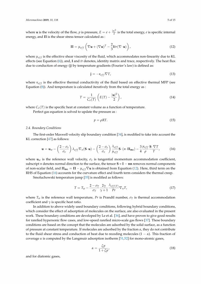
Figures 5 and 6 demonstrate the slip velocity distribution on the bottom wall for Kn = 0.05and 0.1 cases, respectively. As the flow enters the early transition regime, the phenomena of flowseparation, recirculation, and re-attachment disappear. This is because slip velocity on the wallbecomes comparable to the flow velocity. The Knudsen layer thins the shear layer, and fluid followswall direction without separating even at the sudden step corner. It can be observed that NS-MS solver

Micromachines 2019, 10, 118 9 of 15

under-predicts, whereas NS-LMS solver over-predicts the slip velocity when compared to DSMC,throughout the length of the bottom wall. After the incorporation of KL effects, slip velocity valuespredicted by NS-MS solver, move closer to DSMC data, but the improvement is not much significant(∼5.88%), and maximum deviation with DSMC is ∼ 31.57%. On the other hand, results are greatlyimproved for NS-LMS-KL solver, i.e., 10% improvement over NS-LMS solver and deviations within10% with DSMC data. It is noticed that the introduction of KL is more effective when Kngll > 0.05,as the growth of KL thickness increases with increase in Kn. Visualization of KL thickness for variousKn cases is demonstrated in Figure 7, using contours of normalized MFP (β). Thickness of KL isminimal for the Kn = 0.01 case, whereas it almost covers the entire flow domain for Kn = 0.1 case.

2 2.5 3 3.5 4 4.5 5 5.5X ( m)

0

5

10

15

20

25

30

U (

m/s

)

0

0.02

0.04

0.06

0.08

0.1

0.12

0.14

Kn

gll

DSMCNS-MSNS-MS-withKLNS-LMSNS-LMS-withKLKngll

Figure 5. Velocity slip distribution on the bottom wall at Kn = 0.05.

2 2.5 3 3.5 4 4.5 5 5.5X ( m)

0

5

10

15

20

25

U (

m/s

)

0

0.02

0.04

0.06

0.08

0.1

0.12

0.14

Kn

gll

DSMCNS-MSNS-MS-withKLNS-LMSNS-LMS-withKLKngll

Figure 6. Velocity slip distribution on the bottom wall at Kn = 0.1.

Micromachines 2019, 10, 118 10 of 15

(a)

(b)

(c)

Figure 7. Knudsen layer formation in terms of the normalized MFP (β) contours for various Knudsennumbers (obtained using Equation (5)). (a) Kn = 0.01; (b) Kn = 0.05; (c) Kn = 0.1.

3.2. Effect of Change in Inlet Temperature

In this section, the temperature of the flow at the inlet is varied to investigate the effect of KL ontemperature jump on the bottom wall. Simulations are carried out for Kn = 0.01 case with Tin = 500 Kand Tin = 700 K.

Figures 8 and 9 demonstrate the temperature of the fluid on the bottom wall obtained usingdifferent solvers. Local Kn based on velocity gradients is plotted on the secondary y-axis. It is observedthat NS-LMS solver results are closer to DSMC data when compared to NS-MS solver. This is due tothe fact that surface boundary conditions in the DSMC method are based on gas-surface interactions,and particles are adsorbed on the surface and re-emitted. LMS boundary conditions account for theeffect of molecules adsorption on the surface and are able to predict better surface properties than MSboundary conditions.

However, the introduction of KL effects has noticeably improved predictions for both the solvers,NS-MS and NS-LMS. The main reason behind this is that the thermal KL is formed near the wall,whose thickness is more than the momentum KL. It not only modifies the constitutive relation forthe heat flux but also considers the thermal MFP in the calculation of surface temperature jump.The introduction of KL effects has improved NS-MS solver results even in the separation zone, withmaximum relative improvement of 30% for Tin = 500 K case, and 41.05% for Tin = 700 K case w.r.t.DSMC results. NS-LMS solver with and without KL accurately captures the peak temperature valuefor Tin = 500 K case. Location of peak temperature for DSMC is slightly downstream of NS solutions, asflow gradients in DSMC are diffuse. Relative improvement of around 81% is observed for Tin = 700 Kcase solver due to the addition of KL effects over NS-LMS solver.

Micromachines 2019, 10, 118 11 of 15

20 30 40 50 60 70 80 90X (nm)

299

300

301

302

303

304

305

306

307

T (

K)

0

0.01

0.02

0.03

0.04

0.05

0.06

0.07

0.08

0.09

Kn

gll

DSMCNS-MSNS-MS-withKLNS-LMSNS-LMS-withKLKngll

Figure 8. Temperature distribution of the fluid on the bottom wall at Kn = 0.01, Tin = 500 K.

20 30 40 50 60 70 80 90X (nm)

300

302

304

306

308

310

312

314

316

T (

K)

0

0.01

0.02

0.03

0.04

0.05

0.06

0.07

0.08

Kn

gll

DSMCNS-MSNS-MS-withKLNS-LMSNS-LMS-withKLKngll

Figure 9. Temperature distribution of the fluid on the bottom wall at Kn = 0.01, Tin = 700 K.

3.3. Effect of Change in Wall Temperature

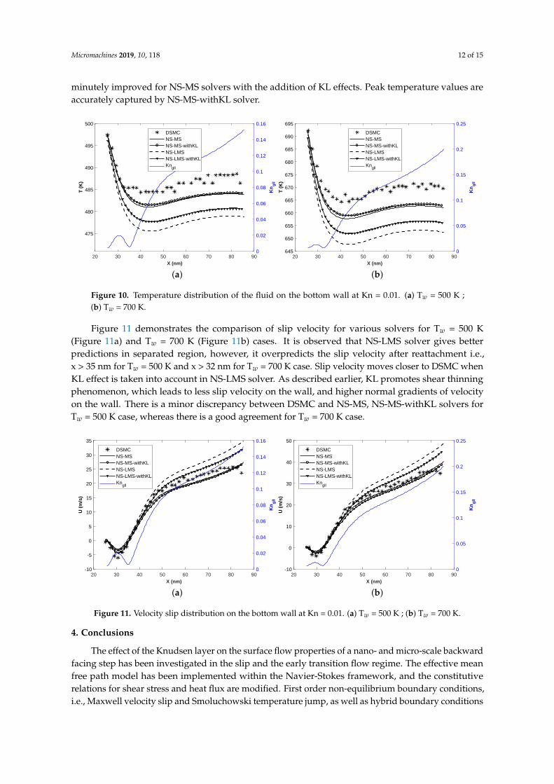
In this section, the temperature of the bottom wall and step has been varied for Kn = 0.01 case.Inlet flow and other walls have the temperature of 300 K. Simulations are carried out by settingtemperature of both the bottom wall and step to 500 K and 700 K.

Figure 10 shows the temperature distribution of fluid on the bottom wall for Tw = 500 K (Figure 10a)and Tw = 700 K (Figure 10b). As wall temperature is higher than the flow temperature, heat istransferred from the wall to the fluid flow, and temperature abruptly drops near the step - bottom wallregion where a separation zone is formed.

It is interesting to note that for this particular case, NS-MS solvers predict better surfacetemperature than NS-LMS solver, unlike previous cases. This can be attributed to the fact that referencetemperature Tw is high, which affects the calculation of α and ζ parameters in Equations (19) and (20),respectively. In LMS boundary conditions, approaching stream of molecules has lower temperaturethan the surface, and high temperature surface adsorbs molecules by fraction of α. These moleculesare re-emitted with T = Tw, which could be the reason that temperature is under-predicted by NS-LMSsolvers. Therefore, LMS boundary conditions are not suitable when temperature gradients are negativeor not uniform. Though NS-LMS solver has deviations w.r.t DSMC data, KL effects have led to therelative improvement of around 24% for Tw = 500 K case and 29% for Tw = 700 K case. Results are

Micromachines 2019, 10, 118 12 of 15

minutely improved for NS-MS solvers with the addition of KL effects. Peak temperature values areaccurately captured by NS-MS-withKL solver.

20 30 40 50 60 70 80 90X (nm)

475

480

485

490

495

500

T (

K)

0

0.02

0.04

0.06

0.08

0.1

0.12

0.14

0.16

Kn

gll

DSMCNS-MSNS-MS-withKLNS-LMSNS-LMS-withKLKngll

(a)

20 30 40 50 60 70 80 90X (nm)

645

650

655

660

665

670

675

680

685

690

695

T (

K)

0

0.05

0.1

0.15

0.2

0.25

Kn

gll

DSMCNS-MSNS-MS-withKLNS-LMSNS-LMS-withKLKngll

(b)

Figure 10. Temperature distribution of the fluid on the bottom wall at Kn = 0.01. (a) Tw = 500 K ;(b) Tw = 700 K.

Figure 11 demonstrates the comparison of slip velocity for various solvers for Tw = 500 K(Figure 11a) and Tw = 700 K (Figure 11b) cases. It is observed that NS-LMS solver gives betterpredictions in separated region, however, it overpredicts the slip velocity after reattachment i.e.,x > 35 nm for Tw = 500 K and x > 32 nm for Tw = 700 K case. Slip velocity moves closer to DSMC whenKL effect is taken into account in NS-LMS solver. As described earlier, KL promotes shear thinningphenomenon, which leads to less slip velocity on the wall, and higher normal gradients of velocityon the wall. There is a minor discrepancy between DSMC and NS-MS, NS-MS-withKL solvers forTw = 500 K case, whereas there is a good agreement for Tw = 700 K case.

20 30 40 50 60 70 80 90X (nm)

-10

-5

0

5

10

15

20

25

30

35

U (

m/s

)

0

0.02

0.04

0.06

0.08

0.1

0.12

0.14

0.16

Kn

gll

DSMCNS-MSNS-MS-withKLNS-LMSNS-LMS-withKLKngll

(a)

20 30 40 50 60 70 80 90X (nm)

-10

0

10

20

30

40

50

U (

m/s

)

0

0.05

0.1

0.15

0.2

0.25

Kn

gll

DSMCNS-MSNS-MS-withKLNS-LMSNS-LMS-withKLKngll

(b)

Figure 11. Velocity slip distribution on the bottom wall at Kn = 0.01. (a) Tw = 500 K ; (b) Tw = 700 K.

4. Conclusions

The effect of the Knudsen layer on the surface flow properties of a nano- and micro-scale backwardfacing step has been investigated in the slip and the early transition flow regime. The effective meanfree path model has been implemented within the Navier-Stokes framework, and the constitutiverelations for shear stress and heat flux are modified. First order non-equilibrium boundary conditions,i.e., Maxwell velocity slip and Smoluchowski temperature jump, as well as hybrid boundary conditions

Micromachines 2019, 10, 118 13 of 15

based on Langmuir adsorption isotherm are effectively modified to incorporate the non-equilibriumeffects associated with KL.

The NS-LMS solver has proven to give better predictions in the separation zone than NS-MSsolver when compared with the benchmark DSMC results. The velocity slip and temperature jumpresults are significantly improved for the NS-LMS method when KL effects are incorporated, implyingthat non-linear effects due to momentum and thermal KL are captured by the proposed method.On the other hand, for the case of negative temperature gradient near the wall, the NS-MS solver haveaccurately predicted the slip velocity and temperature jump and has good agreement with DSMC data,and NS-LMS method have higher deviations with DSMC.

The present results have demonstrated the potential of the effective MFP based approach in themodeling of rarefied nano- and micro-scale gas flows. Although non-linear effects associated withmomentum and thermal KL are captured up to some extent, no strong conclusions can be drawn.In the future, the detailed analysis should be carried out over a wide range of Knudsen numbers,and arbitrary geometries subjected to a range of complex flow conditions.

Author Contributions: Conceptualization, A.B. and H.G.; methodology, A.B.; software, A.B. and H.G.; validation,A.B., H.G. and N.D.; formal analysis, A.B.; investigation, A.B.; writing—original draft preparation, A.B.;writing—review and editing, H.G. and N.D.; funding acquisition, N.D.

Funding: The research was supported by Department of Science and Technology (DST): SERB/F/2684/2014-15and Ministry of Human Resource Development (MHRD) fellowship. The APC was funded by IIT Hyderabad.

Conflicts of Interest: The authors declare no conflict of interest.

References

1. Stops, D. The mean free path of gas molecules in the transition regime. J. Phys. D Appl. Phys. 1970, 3, 685.[CrossRef]

2. Burnett, D. The distribution of molecular velocities and the mean motion in a non-uniform gas. Proc. Lond.Math. Soc. 1936, 2, 382–435. [CrossRef]

3. Grad, H. Note on N-dimensional hermite polynomials. Commun. Pure Appl. Math. 1949, 2, 325–330.[CrossRef]

4. Chapman, S.; Cowling, T.G.; Burnett, D. The Mathematical Theory of Non-Uniform Gases: An Account of TheKinetic Theory of Viscosity, Thermal Conduction and Diffusion in Gases; Cambridge University Press: Cambridge,UK, 1970.

5. Sone, Y. Kinetic Theory and Fluid Dynamics; Springer Science & Business Media: Berlin, Germany, 2012.6. Cercignani, C. Mathematical Methods in Kinetic Theory; Springer: New York, NY, USA, 1969; pp. 232–243.7. Barichello, L.; Siewert, C. The temperature-jump problem in rarefied-gas dynamics. Eur. J. Appl. Math. 2000,

11, 353–364. [CrossRef]8. Barichello, L.B.; Bartz, A.C.R.; Camargo, M.; Siewert, C. The temperature-jump problem for a variable

collision frequency model. Phys. Fluids 2002, 14, 382–391. [CrossRef]9. Su, W.; Wang, P.; Liu, H.; Wu, L. Accurate and efficient computation of the Boltzmann equation for

Couette flow: Influence of intermolecular potentials on Knudsen layer function and viscous slip coefficient.J. Comput. Phys. 2019, 378, 573–590. [CrossRef]

10. Jin, S.; Slemrod, M. Regularization of the Burnett equations via relaxation. J. Stat. Phys. 2001, 103, 1009–1033.[CrossRef]

11. Al-Ghoul, M.; Eu, B.C. Generalized hydrodynamics and microflows. Phys. Rev. E 2004, 70, 016301. [CrossRef]12. Struchtrup, H.; Torrilhon, M. Higher-order effects in rarefied channel flows. Phys. Rev. E 2008, 78, 046301.

[CrossRef]13. Myong, R. Theoretical description of the gaseous Knudsen layer in Couette flow based on the second-order

constitutive and slip-jump models. Phys. Fluids 2016, 28, 012002. [CrossRef]14. Bird, R.B.; Stewart, W.E.; Lightfoot, E.N. Transport Phenomena; John Wiley & Sons: Hoboken, NJ, USA, 2007.15. Bird, G. The DSMC Method; CreateSpace Independent Publishing Platform: Scotts Valley, CA, USA, 2013.

Micromachines 2019, 10, 118 14 of 15

16. White, C.; Borg, M.K.; Scanlon, T.J.; Longshaw, S.M.; John, B.; Emerson, D.; Reese, J.M. dsmcFoam+:An OpenFOAM based direct simulation Monte Carlo solver. Comput. Phys. Commun. 2018, 224, 22–43.[CrossRef]

17. Piekos, E.; Breuer, K. DSMC modeling of micromechanical devices. In Proceedings of the 30th ThermophysicsConference, San Diego, CA, USA, 19–22 June 1995; p. 2089.

18. Oh, C.; Oran, E.; Sinkovits, R. Computations of high-speed, high Knudsen number microchannel flows.J. Thermophys. Heat Transf. 1997, 11, 497–505. [CrossRef]

19. Nance, R.P.; Hash, D.B.; Hassan, H. Role of boundary conditions in Monte Carlo simulation ofmicroelectromechanical systems. J. Thermophys. Heat Transf. 1998, 12, 447–449. [CrossRef]

20. Li, J.M.; Wang, B.X.; Peng, X.F. Wall-adjacent layer analysis for developed-flow laminar heat transfer of gasesin microchannels. Int. J. Heat Mass Transf. 2000, 43, 839–847. [CrossRef]

21. Lockerby, D.A.; Reese, J.M.; Gallis, M.A. Capturing the Knudsen layer in continuum-fluid models ofnonequilibrium gas flows. AIAA J. 2005, 43, 1391–1393. [CrossRef]

22. Cercignani, C.; Frangi, A.; Lorenzani, S.; Vigna, B. BEM approaches and simplified kinetic models for theanalysis of damping in deformable MEMS. Eng. Anal. Bound. Elem. 2007, 31, 451–457. [CrossRef]

23. Lockerby, D.A.; Reese, J.M. On the modelling of isothermal gas flows at the microscale. J. Fluid Mech. 2008,604, 235–261. [CrossRef]

24. Lilley, C.R.; Sader, J.E. Velocity gradient singularity and structure of the velocity profile in the Knudsen layeraccording to the Boltzmann equation. Phys. Rev. E 2007, 76, 026315. [CrossRef]

25. Lilley, C.R.; Sader, J.E. Velocity profile in the Knudsen layer according to the Boltzmann equation. Proc. R.Soc. Lond. A Math. Phys. Eng. Sci. 2008, 464, 2015–2035. [CrossRef]

26. Guo, Z.; Shi, B.; Zheng, C.G. An extended Navier-Stokes formulation for gas flows in the Knudsen layernear a wall. EPL (Europhys. Lett.) 2007, 80, 24001. [CrossRef]

27. Dongari, N.; Zhang, Y.; Reese, J.M. Molecular free path distribution in rarefied gases. J. Phys. D Appl. Phys.2011, 44, 125502. [CrossRef]

28. Dongari, N.; Zhang, Y.; Reese, J.M. Modeling of Knudsen layer effects in micro/nanoscale gas flows.J. Fluids Eng. 2011, 133, 071101. [CrossRef]

29. Guo, Z.; Qin, J.; Zheng, C. Generalized second-order slip boundary condition for nonequilibrium gas flows.Phys. Rev. E 2014, 89, 013021. [CrossRef] [PubMed]

30. Jaiswal, S.; Dongari, N. Implementation of knudsen layer effects in open source cfd solver for effectivemodeling of microscale gas flows. In Proceedings of the 23rd National Heat and Mass Transfer Conferenceand 1st International ISHMT-ASTFE Heat and Mass Transfer Conference IHMTC2015, 17–20 December 2015;pp. 1–8.

31. To, Q.D.; Léonard, C.; Lauriat, G. Free-path distribution and Knudsen-layer modeling for gaseous flows inthe transition regime. Phys. Rev. E 2015, 91, 023015. [CrossRef] [PubMed]

32. Norouzi, A.; Esfahani, J.A. Two relaxation time lattice Boltzmann equation for high Knudsen number flowsusing wall function approach. Microfluid. Nanofluid. 2015, 18, 323–332. [CrossRef]

33. Tu, C.; Qian, L.; Bao, F.; Yan, W. Local effective viscosity of gas in nano-scale channels. Eur. J. Mech.-B/Fluids2017, 64, 55–59. [CrossRef]

34. Maxwell, J.C. On the dynamical theory of gases. Philos. Trans. R. Soc. Lond. 1867, 157, 49–88.35. Smoluchowski von Smolan, M. Ueber wärmeleitung in verdünnten gasen [On heat conduction in diluted

gases]. Annalen der Physik 1898, 300, 101–130. (In German) [CrossRef]36. Le, N.T.; White, C.; Reese, J.M.; Myong, R.S. Langmuir–Maxwell and Langmuir–Smoluchowski boundary

conditions for thermal gas flow simulations in hypersonic aerodynamics. Int. J. Heat Mass Transf. 2012,55, 5032–5043. [CrossRef]

37. Mahdavi, A.M.; Le, N.T.; Roohi, E.; White, C. Thermal rarefied gas flow investigations throughmicro-/nano-backward-facing step: Comparison of dsmc and cfd subject to hybrid slip and jump boundaryconditions. Numer. Heat Transf. Part A Appl. 2014, 66, 733–755. [CrossRef]

38. Weller, H.G.; Tabor, G.; Jasak, H.; Fureby, C. A tensorial approach to computational continuum mechanicsusing object-oriented techniques. Comput. Phys. 1998, 12, 620–631. [CrossRef]

39. Jasak, H. OpenFOAM: a year in review. In Proceedings of the 5th OPENFOAM Workshop, Gothenburg,Sweden, 21–24 June 2010; pp. 21–24.

Micromachines 2019, 10, 118 15 of 15

40. Kurganov, A.; Tadmor, E. New high-resolution central schemes for nonlinear conservation laws andconvection–diffusion equations. J. Comput. Phys. 2000, 160, 241–282. [CrossRef]

41. Kurganov, A.; Noelle, S.; Petrova, G. Semidiscrete central-upwind schemes for hyperbolic conservation lawsand Hamilton–Jacobi equations. SIAM J. Sci. Comput. 2001, 23, 707–740. [CrossRef]

42. Kennard, E.H. Kinetic Theory of Gases, with an Introduction to Statistical Mechanics; McGraw-Hill: New York,NY, USA, 1938.

43. Hirschfelder, J.; Bird, R.B.; Curtiss, C.F. Molecular Theory of Gases and Liquids; Wiley: Hoboken, NY, USA, 1964.44. Anderson, J.D. Hypersonic and High Temperature Gas Dynamics; AIAA: Reston, VA, USA, 2000.45. Vincenti, W.G.; Kruger, C.H. Introduction to Physical Gas Dynamics; Wiley: New York, NY, USA, 1965;

Volume 246.46. Dongari, N. Micro Gas Flows: Modelling the Dynamics of Knudsen Layers. Ph.D. Thesis, University of

Strathclyde, Glasgow, UK, 2012.47. Dongari, N.; Barber, R.W.; Emerson, D.R.; Stefanov, S.K.; Zhang, Y.; Reese, J.M. The effect of Knudsen layers

on rarefied cylindrical Couette gas flows. Microfluid. Nanofluid. 2013, 14, 31–43. [CrossRef]48. Dongari, N.; White, C.; Scanlon, T.J.; Zhang, Y.; Reese, J.M. Effects of curvature on rarefied gas flows between

rotating concentric cylinders. Phys. Fluids 2013, 25, 052003. [CrossRef]49. Sone, Y.; Ohwada, T.; Aoki, K. Evaporation and condensation on a plane condensed phase: Numerical

analysis of the linearized Boltzmann equation for hard-sphere molecules. Phys. Fluids A Fluid Dyn. 1989,1, 1398–1405. [CrossRef]

50. Blazek, J. Computational Fluid Dynamics: Principles and Applications; Butterworth-Heinemann: Oxford, UK, 2015.51. Dushman, S.; Lafferty, J.M.; Pasternak, R. Scientific foundations of vacuum technique. Phys. Today 1962,

15, 53. [CrossRef]52. Myong, R.; Reese, J.; Barber, R.W.; Emerson, D. Velocity slip in microscale cylindrical Couette flow: the

Langmuir model. Phys. Fluids 2005, 17, 087105. [CrossRef]53. Bhattacharya, D.; Eu, B.C. Nonlinear transport processes and fluid dynamics: Effects of thermoviscous

coupling and nonlinear transport coefficients on plane Couette flow of Lennard-Jones fluids. Phys. Rev. A1987, 35, 821. [CrossRef]

54. Wang, M.; Li, Z. Simulations for gas flows in microgeometries using the direct simulation Monte Carlomethod. Int. J. Heat Fluid Flow 2004, 25, 975–985. [CrossRef]

55. Akhlaghi, H.; Roohi, E.; Stefanov, S. A new iterative wall heat flux specifying technique in DSMC forheating/cooling simulations of MEMS/NEMS. Int. J. Therm. Sci. 2012, 59, 111–125. [CrossRef]

c© 2019 by the authors. Licensee MDPI, Basel, Switzerland. This article is an open accessarticle distributed under the terms and conditions of the Creative Commons Attribution(CC BY) license (http://creativecommons.org/licenses/by/4.0/).