Embed Size (px)
Citation preview
DE-AC22-87PC79864
Modeling of Integrated Environmental Control Systemsfor Coal-Fired Power Plants
Final Report
to
U.S. Department of EnergyPittsburgh Energy Technology Center
Pittsburgh, PA 15236
from
Center for Energy and Environmental StudiesCarnegie Mellon University
Pittsburgh, PA 15213
Prepared by
E.S. Rubin, P.I.J.S. Salmento
H.C. FreyA. Abu-BakerM. Berkenpas
May, 1991

i
TABLE OF CONTENTS
TABLE OF CONTENTS ..............................................................................................iLIST OF TABLES.........................................................................................................vLIST OF FIGURES.......................................................................................................viACKNOWLEDGEMENTS ..........................................................................................viii1 INTRODUCTION..............................................................................................12 ENHANCEMENTS TO BASELINE PLANT MODEL.................................3
2.1 Nomenclature.......................................................................................................32.2 Stream Properties and Composition.....................................................................8
2.2.1 Fuel and Other Solid Streams ..................................................................82.2.2 Air and Flue Gas Streams ........................................................................122.2.3 Thermodynamic Data...............................................................................15
2.3 Boiler Efficiency..................................................................................................202.4 Air Preheater ........................................................................................................212.5 Wet FGD Performance.........................................................................................28
2.5.1 Reagent and SO2 Efficiency ....................................................................282.5.2 Water Balance ..........................................................................................292.5.3 Flue Gas Composition and Reheat...........................................................322.5.4 Waste Stream Composition......................................................................342.5.5 Economics Algorithm ..............................................................................35
2.6 Spray Dryer Performance.....................................................................................352.6.1 Reagent and SO2 Efficiency ....................................................................362.6.2 Water Balance ..........................................................................................382.6.3 Flue Gas Composition and Reheat...........................................................382.6.4 Waste Stream Composition......................................................................402.6.5 Economics Algorithm ..............................................................................41
2.7 Power Plant Economics .......................................................................................412.7.1 Base Plant Costs.......................................................................................412.7.2 Pollution Control Equipment Energy Penalties .......................................422.7.3 Pollution Control Equipment Energy Credits ..........................................442.7.4 Total Pollution Control Cost....................................................................46
2.8 Key Financial Parameters ....................................................................................472.8.1 Fixed Charge Factor.................................................................................472.8.2 Levelization Factor ..................................................................................502.8.3 Year-by-Year Revenue Requirement Analysis........................................502.8.4 Accumulated Funds Used During Construction ......................................50
2.9 Conventional Coal Cleaning ................................................................................512.9.1 Introduction..............................................................................................512.9.2 Level 4 Plant Cost....................................................................................512.9.3 Moisture Content of Cleaned Coal ..........................................................51
ii
3 COPPER OXIDE PROCESS MODEL ...........................................................593.1 Nomenclature.......................................................................................................593.2 Introduction..........................................................................................................593.3 Sulfation Reaction Algorithm..............................................................................623.4 Enthalpy Functions ..............................................................................................65
4 NOXSO PROCESS MODEL............................................................................674.1 Nomenclature.......................................................................................................674.2 Introduction..........................................................................................................694.3 Performance Model..............................................................................................724.4 Economic Model..................................................................................................81
4.4.1 Capital Costs ...............................................................................................814.4.2 Operating and Maintenance Costs ..............................................................84
4.5 Deterministic Analysis for the NOXSO Process .................................................854.5.1 Cost Results .............................................................................................864.5.2 NOx Removal Efficiency.........................................................................914.5.3 Effects of Stoichiometry ..........................................................................914.5.4 Process Energy Requirements..................................................................93
4.6 Sensitivity Analysis for the NOXSO Process......................................................934.6.1 Combustion of Acid Plant Gases .............................................................934.6.2 Air Preheater Effects................................................................................944.6.3 Other Process Parameters.........................................................................954.6.4 NOx Reduction Efficiency.......................................................................984.6.5 Sorbent Regenerator Efficiency ...............................................................98
4.7 Conclusion ...........................................................................................................995 ELECTRON BEAM PROCESS MODEL ......................................................102
5.1 Nomenclature.......................................................................................................1025.2 Introduction..........................................................................................................1035.3 Spray Dryer Model Modifications .......................................................................1035.4 Electron Beam Dose ............................................................................................1045.5 Flue Gas Composition .........................................................................................1055.6 Waste Composition..............................................................................................1065.7 Economics Algorithm ..........................................................................................107
6 SULFURIC ACID PLANT MODEL ...............................................................1086.1 Nomenclature.......................................................................................................1086.2 Introduction..........................................................................................................1106.3 Performance Model..............................................................................................1146.4 Economic Model..................................................................................................127
6.4.1 Capital Cost..............................................................................................1276.4.2 Operating and Maintenance Costs ...........................................................129
6.5 Numerical Example .............................................................................................1307 CLAUS PLANT MODEL .................................................................................145
7.1 Nomenclature.......................................................................................................145
iii
7.2 Introduction..........................................................................................................1457.3 Performance Model..............................................................................................1467.4 Economic Model..................................................................................................148
8 FROTH FLOTATION PROCESS MODEL...................................................1508.1 Nomenclature.......................................................................................................1508.2 Introduction..........................................................................................................1518.3 Process Description..............................................................................................1518.4 Froth Flotation Performance Model.....................................................................1538.5 Process Economics...............................................................................................154
9 SELECTIVE AGGLOMERATION PROCESS MODEL.............................1569.1 Nomenclature.......................................................................................................1569.2 Introduction..........................................................................................................1579.3 Process Description..............................................................................................158
9.3.1 Grinding Operation ..................................................................................1589.3.2 Agglomeration and Separation ................................................................1589.3.3 Solvent Recovery and Refuse Thickening ...............................................159
9.4 Performance Model..............................................................................................1609.5 Economic Model..................................................................................................163
9.5.1 Capital Cost..............................................................................................1639.5.2 Operating and Maintenance Cost.............................................................165
9.6 Illustrative Example .............................................................................................1669.6.1 Performance Model..................................................................................1669.6.2 Economic Model......................................................................................168
9.7 Sensitivity Analysis .............................................................................................1739.7.1 Coal Grind................................................................................................1739.7.2 Pulp Density.............................................................................................1769.7.3 Agglomerant Dosage ...............................................................................1769.7.4 Asphalt Dosage ........................................................................................1769.7.5 Effects on Economics ..............................................................................176
10 HEAVY LIQUID SEPARATION PROCESS MODEL.................................17810.1 Nomenclature.................................................................................................17810.2 Introduction....................................................................................................17910.3 Process Description........................................................................................180
10.3.1 Precleaning Subcircuit .............................................................................18010.3.2 Comminution Subcircuit..........................................................................18110.3.3 Heavy Liquid Cyclone (HLC) Subcircuit ................................................18110.3.4 Heavy Liquid Recovery Subcircuit..........................................................182
10.4 Performance Model........................................................................................18310.4.1 Precleaning Subcircuit .............................................................................18310.4.2 Communition Subcircuit..........................................................................18310.4.3 HLC Subcircuit ........................................................................................18310.4.4 HLR Subcircuit ........................................................................................183
iv
10.4.5 Thermal Drier Subcircuit .........................................................................18510.5 Economic Model............................................................................................185
10.5.1 Capital Cost..............................................................................................18610.5.2 Operating and Maintenance Cost.............................................................187
10.6 Illustrative Results .........................................................................................18810.7 Sensitivity Results..........................................................................................190
10.7.1 Illinois Coal..............................................................................................19010.7.2 Pittsburgh No. 8 Coal...............................................................................193
10.8 Numerical Example .......................................................................................19710.8.1 Performance Model..................................................................................19710.8.2 Economic Model......................................................................................200
11 REFERENCES...................................................................................................204APPENDIX.....................................................................................................................1
v
LIST OF TABLES
Table 2-1: Standard Heat of Formation ..........................................................................17Table 2-2: Heats of Reactions .........................................................................................18Table 2-3: Constants for the Specific Heat Correlations ................................................19Table 2-4: Federal Tax Depreciation Schedule...............................................................48Table 4-1: Area Cost Multipliers for NOXSO Process...................................................81Table 4-2: Properties of Illinois No. 6 Coal Used for Case Studies (As-Fired Basis) ....84Table 4-3: NOXSO Performance and Economic Assumptions ......................................85Table 4-4: Financial and Emission Assumptions for Case Studies ................................86Table 4-5: Summary of Total Pollution Control Costs ...................................................87Table 4-6: Breakdown of Cost for NOXSO Process ......................................................88Table 4-7: NOXSO Performance Parameters .................................................................89Table 4-8: Effects of Gas Burner for Sulfuric Acid Plant with the Unwashed Coal ......93Table 4-9: Effects of the Air Preheater for the Unwashed Coal .....................................94Table 6-1: Input Parameters for Sulfuric Acid Plant Numerical Example .....................129Table 9-1: Properties of n-heptane and n-pentane ..........................................................157Table 9-2: Feed Coal and Clean Coal quality .................................................................159Table 9-3: Operating Cost Factors (1980 $) ...................................................................164Table 9-4: Components of Cleaning Cost (1984$ / dry ton of clean coal) .....................168Table 9-5: Breakdown of the Operating and Maintenance Cost s
( 1984$ / dry to of clean coal ) .............................................................................169Table 9-6: Breakdown of the Capital Cost ( Million 1984$ ) .........................................169Table 9.7: Multiple Variable Results on Pittsburgh#8....................................................171Table 9-8: Multiple Variable Results on Illinois #6 .......................................................172Table 9-9: Multiple Variable Results on Upper Freeport ...............................................173Table 10-1: Operating Cost Factors (1980 $) .................................................................186Table 10-2: Feed Coal and Clean Coal quality ...............................................................187Table 10-3: Properties of Heavy Liquids ........................................................................188Table 10-4: The effect of precleaned subcircuit on Pittsburgh coal ...............................189Table 10-5: Quality vs. Coal Size ...................................................................................191Table 10-6: Quality vs. Coal Size ...................................................................................192Table 10-7: Components of Cleaning Cost (1984$ / dry ton of clean coal) ...................200Table 10-8: Breakdown of the Operating and Maintenance Cost ( 1984$ / dry to of clean
coal)......................................................................................................................200Table 10-9: Breakdown of the Capital Cost ( Million 1984$ ) .......................................200
vi
LIST OF FIGURES
Figure 1-1: Schematic of Control Model Technologies .................................................2Figure 2-1: Schematic Diagram of the Gaseous and Solid Streams in IECM ................9Figure 2-2: Schematic Diagram of Air Preheater ...........................................................22Figure 2-3: Schematic Diagram of the Wet FGD Model................................................27Figure 2-4: Flue Gas Specific Heat versus Exit Temperature ........................................30Figure 2-5: Enthalpy Difference between Saturated Steam and Saturated Water at 120•F30Figure 2-6: Saturation Pressure of Water versus Temperature .......................................31Figure 2-7: Evaporated Water versus Temperature ........................................................32Figure 2-8: Schematic Diagram of the Spray Dryer Model............................................36Figure 2-9: Schematic Diagram of a Level 2 Conventional Coal Cleaning Plant ..........55Figure 2-10: Schematic Diagram of a Level 3 Conventional Coal Cleaning Plant ........56Figure 2-11: Schematic Diagram of a Level 4 Conventional Coal Cleaning Plant ........57Figure 3-1: Schematic Diagram of the Copper Oxide Process .......................................60Figure 3-2: Comparison of Experimental and Predicted Copper-to-Sulfur Ratio ..........64Figure 3-3: Typical Device in Copper Oxide Process ....................................................65Figure 4-1: NOXSO Process Diagram............................................................................70Figure 4-2: Simplified Diagram of Mass Flows for Sulfur Compounds ........................72Figure 4-3: Simplified Diagram of Mass Flows for NOx ..............................................74Figure 4-4: Sulfur Removal Efficiency versus Molar Stoichiometry .............................91Figure 4-5: Capital Cost Sensitivity Analysis for Unwashed Coal ................................95Figure 4-6: Total Revenue Requirement Sensitivity Analysis .......................................96Figure 4-7: Effect of NOx Destruction Efficiency in Boiler...........................................98Figure 4-8: Effect of Overall Regenerator Efficiency ....................................................99Figure 5-1: Schematic Diagram of Electron Beam Process............................................101Figure 6-1: Schematic Diagram of Sulfuric Acid Plant..................................................109Figure 6-2: Schematic Diagrams of Inlet Compressor and Gas Burner .........................110Figure 6-3: Inlet Gas Cooling Heat Exchangers .............................................................119Figure 7-1: Schematic Diagram of Claus Sulfur Plant ...................................................144Figure 8-1: Coal Cleaning Plant with Froth Flotation of Fine Stream ...........................150Figure 9-1: Schematic Diagram of Selective Agglomeration Process............................156Figure 9-2: Schematic Diagram of Selective Agglomeration Process with Flow Rates 160Figure 9-3: Components of Total Coal Cost (1984$/dry ton of cleaned coal) ...............170Figure 9-4: Breakdown of Capital Cost (Million 1984$) ...............................................170Figure 9-5: Cleaning Cost (1984$/dry ton of cleaned coal) vs. Sulfur Reduction (%) on
Different Grind Size.............................................................................................175Figure 9-6: Cleaning Cost (1984$/dry ton of cleaned coal) vs. Sulfur Reduction (%) on
Different Pulp Density .........................................................................................175Figure 10-1: Heavy Liquid Cyclone Subcircuit (HLC) ..................................................179Figure 10-2: Heavy Liquid Recovery Subcircuit (HLR) ................................................180

vii
Figure 10-3: Illinois #6: Grind Size vs. Grade Recovery ...............................................190Figure 10-4: Illinois #6: Effect of Solid Concentration on Performance........................190Figure 10-5: Pittsburgh: Grind Size vs. Grade Recovery ...............................................193Figure 10-6: Pittsburgh: Effect of Solid Concentration on Performance .......................193Figure 10-7: Grade / Recovery vs. Aclean .......................................................................194Figure 10-8: Grade / Recovery vs. PSclean .....................................................................195Figure 10-9: Components of Total Coal Cost ................................................................201Figure 10-10: Components of Capital Cost ...................................................................201

viii
ACKNOWLEDGEMENTS
The work described in this report was carried out under Contract No. DE-AC22-87PC79864for the U.S. Department of Energy, Pittsburgh Energy Technology Center (DOE/PETC). Theauthors acknowledge the support and assistance of Mr. Charles Drummond, Mr. Richard Hucko,Dr. Soung Kim, Mr. Charles Schmidt and Ms. Felixa Eskey of DOE/PETC in the conduct of thisresearch.
1
1 INTRODUCTION
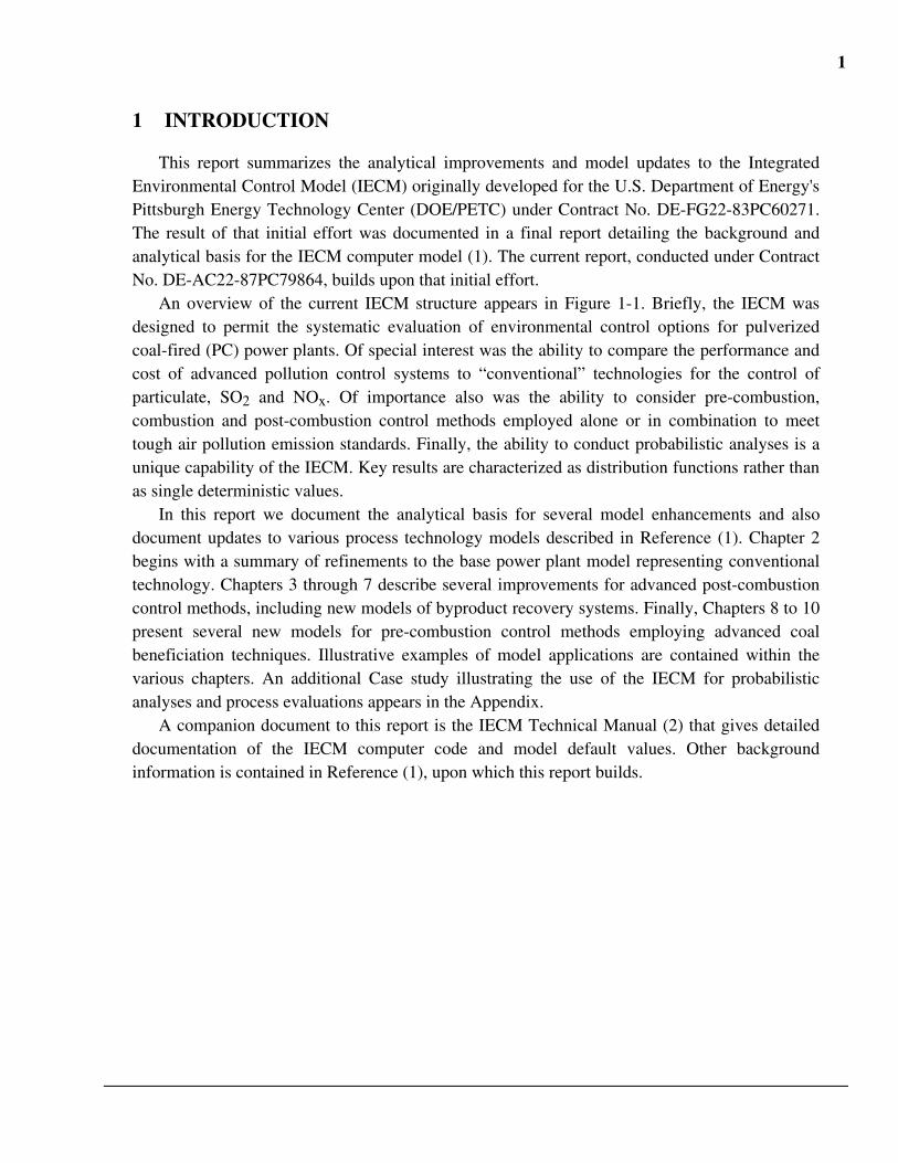
This report summarizes the analytical improvements and model updates to the IntegratedEnvironmental Control Model (IECM) originally developed for the U.S. Department of Energy'sPittsburgh Energy Technology Center (DOE/PETC) under Contract No. DE-FG22-83PC60271.The result of that initial effort was documented in a final report detailing the background andanalytical basis for the IECM computer model (1). The current report, conducted under ContractNo. DE-AC22-87PC79864, builds upon that initial effort.
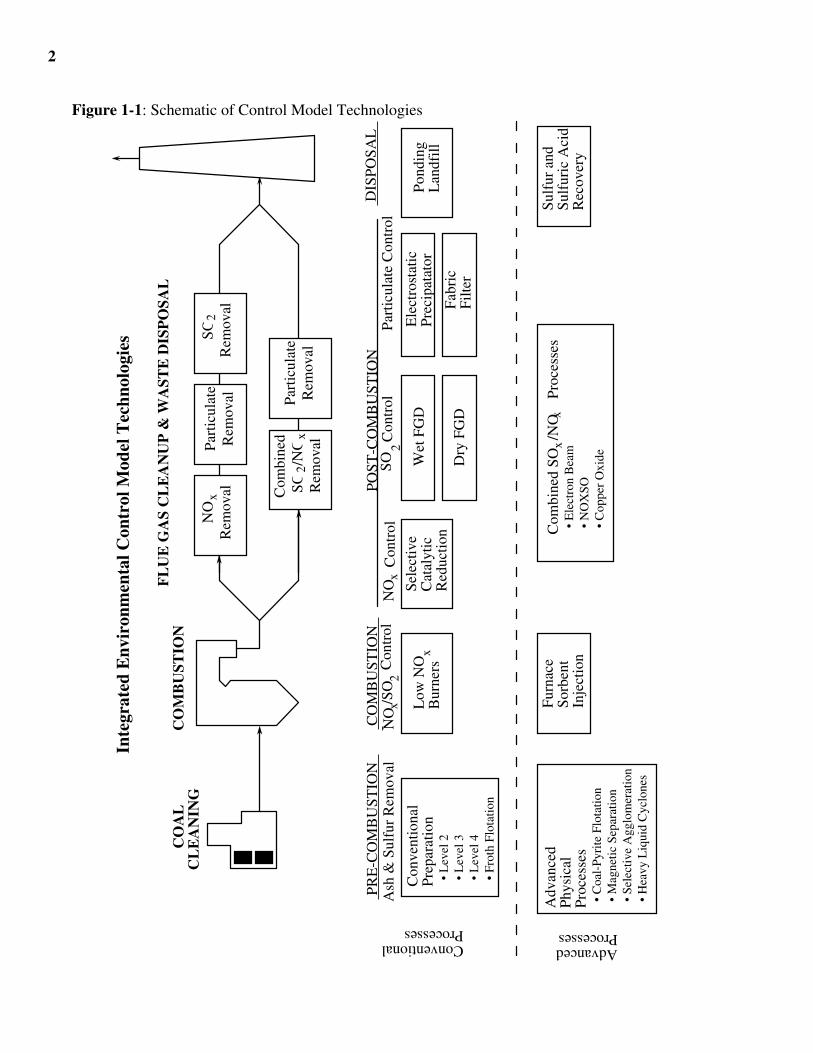
An overview of the current IECM structure appears in Figure 1-1. Briefly, the IECM wasdesigned to permit the systematic evaluation of environmental control options for pulverizedcoal-fired (PC) power plants. Of special interest was the ability to compare the performance andcost of advanced pollution control systems to “conventional” technologies for the control ofparticulate, SO2 and NOx. Of importance also was the ability to consider pre-combustion,combustion and post-combustion control methods employed alone or in combination to meettough air pollution emission standards. Finally, the ability to conduct probabilistic analyses is aunique capability of the IECM. Key results are characterized as distribution functions rather thanas single deterministic values.
In this report we document the analytical basis for several model enhancements and alsodocument updates to various process technology models described in Reference (1). Chapter 2begins with a summary of refinements to the base power plant model representing conventionaltechnology. Chapters 3 through 7 describe several improvements for advanced post-combustioncontrol methods, including new models of byproduct recovery systems. Finally, Chapters 8 to 10present several new models for pre-combustion control methods employing advanced coalbeneficiation techniques. Illustrative examples of model applications are contained within thevarious chapters. An additional Case study illustrating the use of the IECM for probabilisticanalyses and process evaluations appears in the Appendix.
A companion document to this report is the IECM Technical Manual (2) that gives detaileddocumentation of the IECM computer code and model default values. Other backgroundinformation is contained in Reference (1), upon which this report builds.
2
Figure 1-1: Schematic of Control Model Technologies
Low
NO
x
CO
MB
UST
ION
N
Ox/
SO2
Con
trol
Bur
ners
PR
E-C
OM
BU
STIO
N
Ash
& S
ulfu
r R
emov
alPO
ST-C
OM
BU
STIO
N
N
Ox
Con
trol
Part
icul
ate
Con
trol
Wet
FG
D
Dry
FG
D
xx
Conventional Processes
Advanced Processes
SO2
Con
trol
NO
R
emov
alxPa
rtic
ulat
e R
emov
alSO
R
emov
al2
Com
bine
d S
O /
NO
R
emov
alx
2Pa
rtic
ulat
e R
emov
al
FL
UE
GA
S C
LE
AN
UP
& W
AST
E D
ISP
OSA
LC
OM
BU
STIO
NC
OA
L
CL
EA
NIN
G
Inte
grat
ed E
nvir
onm
enta
l Con
trol
Mod
el T
echn
olog
ies
Adv
ance
d Ph
ysic
al
Proc
esse
s •
Coa
l-Py
rite
Flo
tatio
n •
Mag
netic
Sep
arat
ion
• S
elec
tive
Agg
lom
erat
ion
• H
eavy
Liq
uid
Cyc
lone
s
Con
vent
iona
l Pr
epar
atio
n •
Lev
el 2
•
Lev
el 3
•
Lev
el 4
•
Fro
th F
lota
tion
Sele
ctiv
e C
atal
ytic
R
educ
tion
Ele
ctro
stat
ic
Prec
ipat
ator
Fabr
ic
Filte
r
Com
bine
d SO
/N
O
Pro
cess
es
• E
lect
ron
Bea
m
• N
OX
SO
• C
oppe
r O
xide
DIS
POSA
L
Pond
ing
Lan
dfill
Furn
ace
Sor
bent
In
ject
ion
Sul
fur
and
Sulf
uric
Aci
d R
ecov
ery
3
2 ENHANCEMENTS TO BASELINE PLANT MODEL
The “baseline” power plant in the IECM is a plant consisting of a conventional PC boilerwith low NOx burners plus a selective catalytic reduction (SCR) system for NOx control, either awet or dry flue gas desulfurization (FGD) system for SO2 removal and (depending on the choiceof FGD system) either a cold-side electrostatic precipitator (ESP) or fabric filter for particulatecontrol. Physical coal cleaning with post-combustion controls also is part of the baseline system.
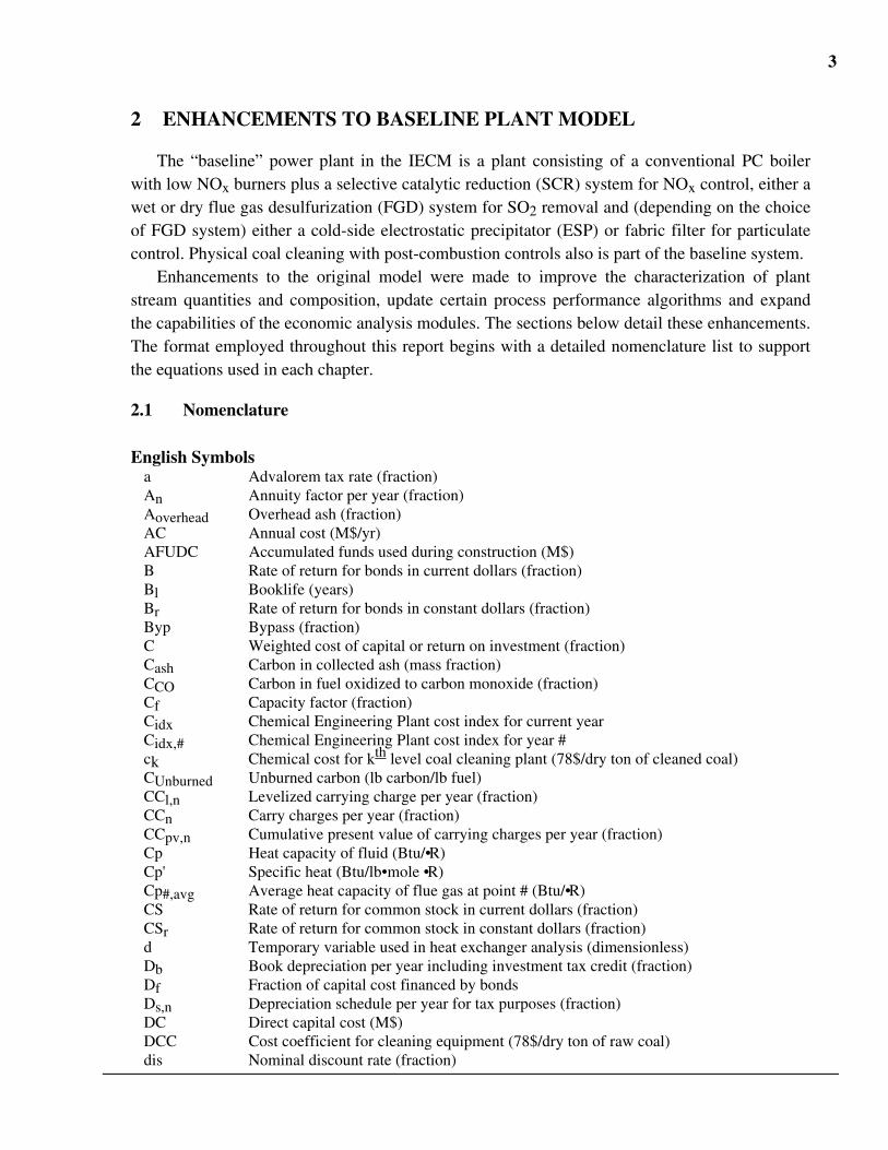
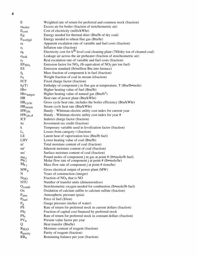
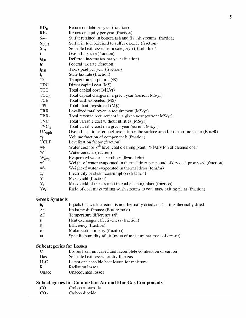
Enhancements to the original model were made to improve the characterization of plantstream quantities and composition, update certain process performance algorithms and expandthe capabilities of the economic analysis modules. The sections below detail these enhancements.The format employed throughout this report begins with a detailed nomenclature list to supportthe equations used in each chapter.
2.1 Nomenclature
English Symbolsa Advalorem tax rate (fraction)An Annuity factor per year (fraction)Aoverhead Overhead ash (fraction)AC Annual cost (M$/yr)AFUDC Accumulated funds used during construction (M$)B Rate of return for bonds in current dollars (fraction)Bl Booklife (years)Br Rate of return for bonds in constant dollars (fraction)Byp Bypass (fraction)C Weighted cost of capital or return on investment (fraction)Cash Carbon in collected ash (mass fraction)CCO Carbon in fuel oxidized to carbon monoxide (fraction)Cf Capacity factor (fraction)Cidx Chemical Engineering Plant cost index for current yearCidx,# Chemical Engineering Plant cost index for year #ck Chemical cost for kth level coal cleaning plant (78$/dry ton of cleaned coal)CUnburned Unburned carbon (lb carbon/lb fuel)CCl,n Levelized carrying charge per year (fraction)CCn Carry charges per year (fraction)CCpv,n Cumulative present value of carrying charges per year (fraction)Cp Heat capacity of fluid (Btu/•R)Cp' Specific heat (Btu/lb•mole •R)Cp#,avg Average heat capacity of flue gas at point # (Btu/•R)CS Rate of return for common stock in current dollars (fraction)CSr Rate of return for common stock in constant dollars (fraction)d Temporary variable used in heat exchanger analysis (dimensionless)Db Book depreciation per year including investment tax credit (fraction)Df Fraction of capital cost financed by bondsDs,n Depreciation schedule per year for tax purposes (fraction)DC Direct capital cost (M$)DCC Cost coefficient for cleaning equipment (78$/dry ton of raw coal)dis Nominal discount rate (fraction)
4
E Weighted rate of return for preferred and common stock (fraction)eboiler Excess air for boiler (fraction of stoichiometric air)Ecost Cost of electricity (mills/kWhr)Ed Energy needed for thermal drier (Btu/lb of dry coal)Ewetfgd Energy needed to reheat flue gas (Btu/hr)ef Apparent escalation rate of variable and fuel costs (fraction)ei Inflation rate (fraction)ek Electricity cost for kth level coal cleaning plant (78$/dry ton of cleaned coal)eleak Leakage air across the air preheater (fraction of stoichiometric air)er Real escalation rate of variable and fuel costs (fraction)EFNO2 Emission factor for NOx (lb equivalent of NO2 per ton fuel)ES Emission standard (lb/million Btu into furnace)fk Mass fraction of component k in fuel (fraction)fsi Weight fraction of coal in stream i(fraction)FCF Fixed charge factor (fraction)hj(T) Enthalpy of component j in flue gas at temperature, T (Btu/lb•mole)Hhv Higher heating value of fuel (Btu/lb)Hhvnatgas Higher heating value of natural gas (Btu/ft3)HR Heat rate of power plant (Btu/kWhr)HRcycle Gross cycle heat rate, includes the boiler efficiency (Btu/kWhr)HRsteam Steam cycle heat rate (Btu/kWhr)HWidx Handy - Whitman electric utility cost index for current yearHWidx,# Handy - Whitman electric utility cost index for year #ICF Indirect charge factor (fraction)itc Investment tax credit (fraction)k Temporary variable used in levelization factor (fraction)Li Losses from category i (fraction)LE Latent heat of vaporization loss (Btu/lb fuel)LHV Lower heating value of coal (Btu/lb)m' Total moisture content of coal (fraction)mi' Inherent moisture content of coal (fraction)ms' Surface moisture content of coal (fraction)m#,j Pound moles of component j in gas at point # (lb•mole/lb fuel)m#,j Molar flow rate of component j at point # (lb•mole/hr)M#,j Mass flow rate of component j at point # (tons/hr)MWg Gross electrical output of power plant (MW)N Years of construction (integer)NNO Fraction of NOx that is NONTU Number of transfer units (dimensionless)Ocomb Stoichiometric oxygen needed for combustion (lb•mole/lb fuel)Ox Oxidation of calcium sulfite to calcium sulfate (fraction)Patm Atmospheric pressure (psia)Pfuel Price of fuel ($/ton)Pg Guage pressure (inches of water)PS Rate of return for preferred stock in current dollars (fraction)PSf Fraction of capital cost financed by preferred stockPSr Rate of return for preferred stock in constant dollars (fraction)PVn Present value factor per yearQ Heat transfer (Btu/hr)RH2O Moisture content of reagent (fraction)Rpurity Purity of reagent (fraction)RBn Remaining balance per year (fraction)
5
RDn Return on debt per year (fraction)REn Return on equity per year (fraction)Sret Sulfur retained in bottom ash and fly ash streams (fraction)SSO2 Sulfur in fuel oxidized to sulfur dioxide (fraction)SEi Sensible heat losses from category i (Btu/lb fuel)t Overall tax rate (fraction)td,n Deferred income tax per year (fraction)tf Federal tax rate (fraction)tp,n Taxes paid per year (fraction)ts State tax rate (fraction)T# Temperature at point # (•R)TDC Direct capital cost (M$)TCC Total capital cost (M$/yr)TCCn Total capital charges in a given year (current M$/yr)TCE Total cash expended (M$)TPI Total plant investment (M$)TRR Levelized total revenue requirement (M$/yr)TRRn Total revenue requirement in a given year (current M$/yr)TVC Total variable cost without utilities (M$/yr)TVCn Total variable cost in a given year (current M$/yr)UAaph Overall heat transfer coefficient times the surface area for the air preheater (Btu/•R)vj Volume fraction of component k (fraction)VCLF Levelization factor (fraction)wk Water cost for kth level coal cleaning plant (78$/dry ton of cleaned coal)W Water content (fraction)Wevp Evaporated water in scrubber (lb•mole/hr)w' Weight of water evaporated in thermal drier per pound of dry coal processed (fraction)w'e Weight of water evaporated in thermal drier (tons/hr)xi Electricity or steam consumption (fraction)Y Mass yield (fraction)Yi Mass yield of the stream i in coal cleaning plant (fraction)Yod Ratio of coal mass exiting wash streams to coal mass exiting plant (fraction)
Greek Symbolsδi Equals 0 if wash stream i is not thermally dried and 1 if it is thermally dried.∆h Enthalpy difference (Btu/lb•mole)∆T Temperature difference (•F)ε Heat exchanger effectiveness (fraction)η Efficiency (fraction)σ Molar stoichiometry (fraction)ω Specific humidity of air (mass of moisture per mass of dry air)
Subcategories for LossesC Losses from unburned and incomplete combustion of carbonGas Sensible heat losses for dry flue gasH2O Latent and sensible heat losses for moistureR Radiation lossesUnacc Unaccounted losses
Subcategories for Combustion Air and Flue Gas ComponentsCO Carbon monoxideCO2 Carbon dioxide
6
H2O MoistureN2 NitrogenNO Nitrogen oxideNO2 Nitrogen dioxideO2 OxygenSO2 Sulfur dioxideSO3 Sulfur trioxide
Subcategories for Fuel ComponentsAsh AshC CarbonH Hydrogen (monatomic)H2O MoistureN Nitrogen (monatomic)O Oxygen (monatomic)
Subcategories for Natural Gas ComponentsCH4 MethaneC2H6 EthaneCO2 Carbon dioxideN2 NitrogenO2 Oxygen
Subcategories for Solid Stream ComponentsAsh AshCaO LimeCaCO3 LimestoneCaSO3•.5H2O Hydrated calcium sulfiteCaSO4 Calcium SulfateCaSO4•2H2O Hydrated calcium sulfateH2O Water or MoistureMisc Miscellaneous
Subcategories for Stream Locationapho Exiting air preheater on combustion air sidebotash Bottom ash streamecono Exiting the economizerfdfan Exiting forced draft fanfg1 Located at point 1 in flue gas stream (see Figure 2-1)fg2 Located at point 2 in flue gas stream (see Figure 2-1)fg3 Located at point 3 in flue gas stream (see Figure 2-1)fgaphi Entering air preheater on flue gas sidefgapho Exiting air preheater on flue gas sidefuel Fuel streamfurn In furnace after combustionleak Leakage across air preheaterstack Entering stackunc “Uncorrected” flue gas temperature
Subcategories for Utility Consumptionc Cooling systemf Fans
7
misc Miscellaneousp Pulverizerssp Steam pumps
Subcategories for Economic Variablesfuel Fuel chargesnon Non fuel chargesutil Utility charges, i.e. steam and electricity consumption (M$/yr)w/o cc Without coal cleaningw/o util Without utility charges
Subcategories for FGD Variablesevp Evaporatedmax Maximummin Minimumreag Reagentrem Removedrh ReheaterS Sulfur or sulfur compoundsd Spray dryersat Saturationsludge Sludge exiting bottom of scrubberSO2 Sulfur dioxidestd Based on emission standardTSP Total suspended particulates in flue gas
General Subcategoriesaph Air preheaterbp Base power plantc Coal exiting the washing equipmentcredit Creditd Thermal drierdelta Change between current and originalexit Exiting deviceff Fabric filterin Entering devicenatgas Natural gasnew Current or modifiedo Final product of coal cleaning plantorig Original or without pollution control equipmentoil Fuel oilop Overall power plant (including pollution control equipment)out Exiting devicep Cleaning equipment in coal cleaning plantpce Pollution control equipmentref Refuse stream in coal cleaning plantROM Run-of-mine coalt Overall coal cleaning planttotal Sum or total
8
2.2 Stream Properties and Composition
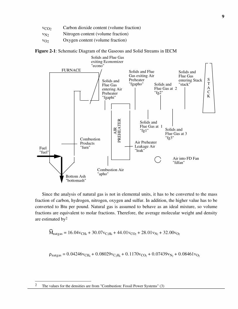
This section describes how the IECM calculates the quantity and quality of solid and gaseousstreams in fossil-fuel fired power plants. A schematic of the solid and gaseous streams for thebase power plant is shown in Figure 2-1. These basic streams are always present in the model. Asthe plant is configured with pollution control equipment, additional streams are created and theequations defining the streams in Figure 2-1 may be modified.
The phrases in quotation marks in Figure 2-1 are the stream labels. They are used as variablesubscripts in this documentation to show the variable location in the power plant. For example,the variable Tfgaphi refers the temperature of the flue gas at the air preheater inlet. The subscripts“fg1”, “fg2” and “fg3” refer to locations downstream from the air preheater. Pollution controlequipment is placed between these locations. For example, an ESP is placed between “fgapho”and “fg1”. The variables at “fgapho” and “fg1” are respectively the inlet and outlet variables forthe ESP. The equations for some variables at “fg1” are redefined to reflect the changes caused bythe ESP. The following section describes in more detail the stream variables and their equations.
2.2.1 Fuel and Other Solid StreamsThis section describes the fuel and other solid streams in the base power plant. The IECM
tracks the following chemical compounds in most solid streams (tons per hour): final ash, lime,limestone, hydrated calcium sulfite, calcium sulfate, hydrated calcium sulfate, moisture andmiscellaneous1. The total mass flow of any stream is the sum of these chemical compounds. Forthe fuel stream, the total mass flow rate is determined instead of the mass flow rates of thechemical components.
Oil or natural gas is added to coal in the IECM as boiler fuels. The model requires thefollowing property variables for coal and oil:
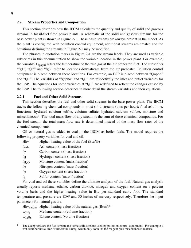
Hhv Higher heating value of the fuel (Btu/lb)fAsh Ash content (mass fraction)fC Carbon content (mass fraction)fH Hydrogen content (mass fraction)fH2O Moisture content (mass fraction)fN Nitrogen content (mass fraction)fO Oxygen content (mass fraction)fS Sulfur content (mass fraction)For coal and oil these variables define the ultimate analysis of the fuel. Natural gas analysis
usually reports methane, ethane, carbon dioxide, nitrogen and oxygen content on a percentvolume basis and the higher heating value in Btu per standard cubic foot. The standardtemperature and pressure are 80•F and 30 inches of mercury respectively. Therefore the inputparameters for natural gas are:
Hhvnatgas Higher heating value of the natural gas (Btu/ft3)
vCH4 Methane content (volume fraction)vC2H6 Ethane content (volume fraction)
1 The exceptions are the fuel stream and some solid streams used by pollution control equipment. For example a
wet scrubber has a lime or limestone slurry, which only contains the reagent plus miscellaneous material.
9
vCO2 Carbon dioxide content (volume fraction)vN2 Nitrogen content (volume fraction)vO2 Oxygen content (volume fraction)
Figure 2-1: Schematic Diagram of the Gaseous and Solid Streams in IECM
Air into FD Fan "fdfan"
Combustion Air "apho"
Air Preheater Leakage Air "leak"
Solids and Flue Gas exiting Economizer "econo"
Solids and Flue Gas entering Air Preheater "fgaphi"
Solids and Flue Gas exiting Air Preheater "fgapho"
Solids and Flue Gas at 1 "fg1"
Solids and Flue Gas at 2 "fg2"
Solids and Flue Gas at 3 "fg3"
Solids and Flue Gas entering Stack "stack"
FURNACE
AIR
P
RE
HE
AT
ER
Fuel "fuel"
Bottom Ash "bottomash"
Combustion Products "furn"
S T A C K
Since the analysis of natural gas is not in elemental units, it has to be converted to the massfraction of carbon, hydrogen, nitrogen, oxygen and sulfur. In addition, the higher value has to beconverted to Btu per pound. Natural gas is assumed to behave as an ideal mixture, so volumefractions are equivalent to molar fractions. Therefore, the average molecular weight and densityare estimated by2
Mnatgas = 16.04vCH4 + 30.07vC2H6 + 44.01vCO2 + 28.01vN2 + 32.00vO2
ρnatgas = 0.04246vCH4 + 0.08029vC2H6
+ 0.1170vCO2 + 0.07439vN2
+ 0.08461vO2
2 The values for the densities are from "Combustion: Fossil Power Systems" (3)
10
The higher heating value on a mass basis can be determined by dividing the higher heatingvalue on a volume basis by the density.
Hhv = Hhvnatgas
ρnatgas
The mass fractions of carbon, hydrogen, nitrogen and oxygen are found by determining themass of the individual components (i.e. carbon, hydrogen, etc.) and dividing by the averagemolecular weight. Since the natural gas is assumed to be free of ash, sulfur and moisture, thesevalues are set to zero.
fC = 12.01vCH4 + 24.02vC2H4 + 12.01vCO2
Mnatgas
fH = 4.04vCH4 + 6.06vC2H4
Mnatgas
fN = 28.01vN2
Mnatgas
fO = 32.00vO2
+ 32.00vCO2
Mnatgas
fAsh = fS = fH2O = 0
With the fuel characteristics it is possible to calculate the mass flow rates and composition ofthe gaseous and solid streams in the power plant. The mass flow rate of fuel must be calculatedfirst.
The base power plant is sized to produce a specified amount of electricity, MWg, which is theamount of electricity that the generators produce. The amount of fuel needed to produce the grosselectric capacity, MWg, depends upon the gross cycle heat rate, boiler efficiency and higherheating value of the fuel. It is determined by
Mfuel = MWg HRcycle
2 Hhv
where
HRcycle = HRsteamηboiler
11
The gross electrical capacity, steam cycle heat rate and the higher heating value of the fuelare input parameters. The boiler efficiency is calculated and described in more detail in Section2.3.
With the mass flow rate of fuel determined, it is now possible to determine the mass flowrates of the other solids streams in the power (e.g. the bottom ash or flyash). The solids producedby combustion are from three sources: ash in the fuel, sulfur retained in the ash and any unburnedcarbon. The mass from sulfur in the ash and the unburned carbon is accounted for in the variableMfurn,misc. The base power plant does not inject lime or limestone slurries into the flue gasstream. Therefore, mass flow rates of lime, limestone, calcium sulfate, hydrated calcium sulfatecalcium sulfite and moisture are zero.
Mfurn,ash = fAshMfuel
;
Mfurn,Misc = fSSret + fCCUnburned Mfuel
Mfurn,k = 0 for k = CaO, CaCO3, CaSO3•0.5H2O, CaSO4, CaSO4•2H2O, H2O
The unburned carbon is a solid entrained in the bottom ash and flyash streams. Utilitiesmeasure the fraction of carbon in their collected ash streams. This value is called the percentcarbon in refuse and is used in the following formula to determine the amount of unburnedcarbon per pound of fuel.
CUnburned = fash Cash1 - Cash
(2.1)
The solids produced by combustion can either exit the furnace with the flue gas or drop outthe bottom of the furnace. The fraction that exists with the flue gas is the overhead ash fractionand is a function of the furnace design and coal rank. The bottom ash flow rate is determined by
Mbotash,k = Mfurn,k (1 - Aoverhead) for all k
The solids exiting the economizer is equal to the overhead ash fraction times the solids
produced by combustion.
Mecono,k = Mfurn,k Aoverhead for all k
For the base power plant, no pollution control equipment can change the mass flow rates of
solids in the flue gas. The mass flow rates of solids at each location are the mass flow rate ofsolids at the previous location. When pollution control equipment is added the definitions ofthese variables change depending upon the specific choice of equipment.
12
Mstack,k = Mfg3,k = Mfg2,k = Mfg1,k = Mfgapho,k = Mfgaphi,k = Mecono,k for all k
2.2.2 Air and Flue Gas StreamsThis section describes the gaseous streams in the base power plant. The IECM tracks the
following chemical compounds in all gaseous streams (lb•mole/lb fuel and lb•mole/hour):diatomic nitrogen, diatomic oxygen, moisture, carbon dioxide, carbon monoxide, sulfur dioxide,sulfur trioxide, nitrogen oxide and nitrogen dioxide. At every location in Figure 2-1, the IECMdetermines the gaseous stream flow rate in lb•mole/lb fuel and lb•mole/hour. The gaseous streamvariables with units of lb•mole/lb fuel describe the gas stream created by the base power plant.They do not change as pollution control equipment is added. These variables are needed bydifferent algorithms in the IECM for comparison with the base power plant3. The gaseous streamvariables with units of lb•mole/hour describe the gas stream for the current power plantconfiguration.
The gas streams are assumed to act as ideal mixtures and obey the ideal gas law. Therefore,the total value of a stream property can be determined by summing the values of the property ofthe individual components. Since the gases obey the ideal gas law, the enthalpy is a function oftemperature only. The enthalpy functions are described in more detail in Section 2.2.3. The totalvolumetric flow rate and enthalpy of a gaseous stream are determined by
V = 1545 T144 * 60 (Patm + 0.036127Pg)
mjj=1
9
h(T) = hj(T)j=1
9
The IECM assumes that dry air consist of 79% nitrogen and 21% oxygen. The specifichumidity is an input parameter. The volumetric fraction of nitrogen, oxygen and moisture can bedetermined from
vN2 = 0.791 + 0.79*28.01 + 0.21*32.00
18.02 ω
= 0.791 + 1.601ω
vH2O = 1.601ω1 + 1.601ω
;
vO2 = 0.211 + 1.601ω
The amount of oxygen needed for stoichiometric combustion of the fuel is the sum of the
oxygen needed to convert of carbon to carbon dioxide, hydrogen to water and sulfur to sulfur
3 The boiler efficiency algorithm uses the gaseous stream variables in units of lb•mole/lb fuel to prevent a cyclic
dependency between the boiler efficiency and the mass flow rate of fuel.
13
dioxide minus any oxygen in the fuel. To minimize incomplete combustion losses, thecombustion air entering the furnace is more than the stoichiometric air requirement. Thisadditional air is called excess air and is an input parameter.
Ocomb = fC12.01
+ fH1.01
+ fS32.06
- fO16.00
mapho,N2 = vN2(1 + eboiler)Ocomb
vO2
;
mapho,H2O = vH2O(1 + eboiler)Ocomb
vO2
mapho,O2 = (1 + eboiler)Ocomb
;
mapho,j = 0
for j = CO2,CO,SO2,SO3,NO,NO2
mapho,j = 2000 Mfuel mapho,j
The leakage air across the air preheater is based upon the stoichiometric air requirement and
is an input parameter. The air entering the forced draft fans is the sum of the leakage air and theair entering the furnace.
mleak,N2 = vN2(1 + eleak)Ocomb
vO2
;
mleak,H2O = vH2O(1 + eleak)Ocomb
vO2
mleak,O2 = (1 + eleak)Ocomb
;
mleak,j = 0
for j = CO2, CO, NO, NO2, SO2, SO3
mleak,j = 2000 Mfuel mleak,j
mfdfan,j = mapho,j + mleak,j
;
mfdfan,j = mapho,j + mleak,j
The products of combustion are determined by specifying extent of combustion for carbon,
sulfur and nitrogen and an emission factor for NO2. The carbon in the fuel can oxides to carbonmonoxide or carbon dioxide or it can remain unburned. The amount of unburned carbon,CUnburned, is determined with Equation (2.1). The amount of carbon monoxide is determined bythe input parameter CCO, the fraction of carbon that oxidizes to carbon monoxide. The sulfur inthe fuel can oxidize to either sulfur dioxide or sulfur trioxide. It also can be captured in the ash.The amount sulfur retained in the ash is determined by the input parameter, Sret. The amount of
14
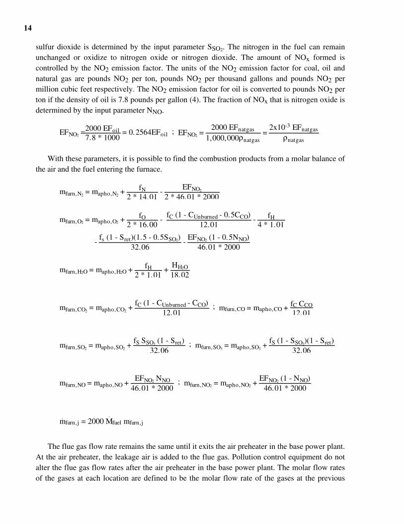
sulfur dioxide is determined by the input parameter SSO2. The nitrogen in the fuel can remainunchanged or oxidize to nitrogen oxide or nitrogen dioxide. The amount of NOx formed iscontrolled by the NO2 emission factor. The units of the NO2 emission factor for coal, oil andnatural gas are pounds NO2 per ton, pounds NO2 per thousand gallons and pounds NO2 permillion cubic feet respectively. The NO2 emission factor for oil is converted to pounds NO2 perton if the density of oil is 7.8 pounds per gallon (4). The fraction of NOx that is nitrogen oxide isdetermined by the input parameter NNO.
EFNO2 =2000 EFoil7.8 * 1000
= 0.2564EFoil
;
EFNO2 = 2000 EFnatgas
1,000,000ρnatgas =
2x10⁻³ EFnatgas
ρnatgas
With these parameters, it is possible to find the combustion products from a molar balance ofthe air and the fuel entering the furnace.
mfurn,N2 = mapho,N2
+ fN2 * 14.01
- EFNO2
2 * 46.01 * 2000
mfurn,O2 = mapho,O2 + fO2 * 16.00
- fC (1 - CUnburned - 0.5CCO)
12.01 - fH
4 * 1.01
- fs (1 - Sret)(1.5 - 0.5SSO2)
32.06 -
EFNO2 (1 - 0.5NNO)46.01 * 2000
mfurn,H2O = mapho,H2O + fH2 * 1.01
+ HH2O
18.02
mfurn,CO2 = mapho,CO2
+ fC (1 - CUnburned - CCO)
12.01
;
mfurn,CO = mapho,CO + fC CCO
12.01
mfurn,SO2 = mapho,SO2
+ fS SSO2
(1 - Sret)32.06
;
mfurn,SO3 = mapho,SO3
+ fS (1 - SSO2
)(1 - Sret)32.06
mfurn,NO = mapho,NO + EFNO2 NNO
46.01 * 2000
;
mfurn,NO2 = mapho,NO2 + EFNO2 (1 - NNO)
46.01 * 2000
mfurn,j = 2000 Mfuel mfurn,j
The flue gas flow rate remains the same until it exits the air preheater in the base power plant.At the air preheater, the leakage air is added to the flue gas. Pollution control equipment do notalter the flue gas flow rates after the air preheater in the base power plant. The molar flow ratesof the gases at each location are defined to be the molar flow rate of the gases at the previous
15
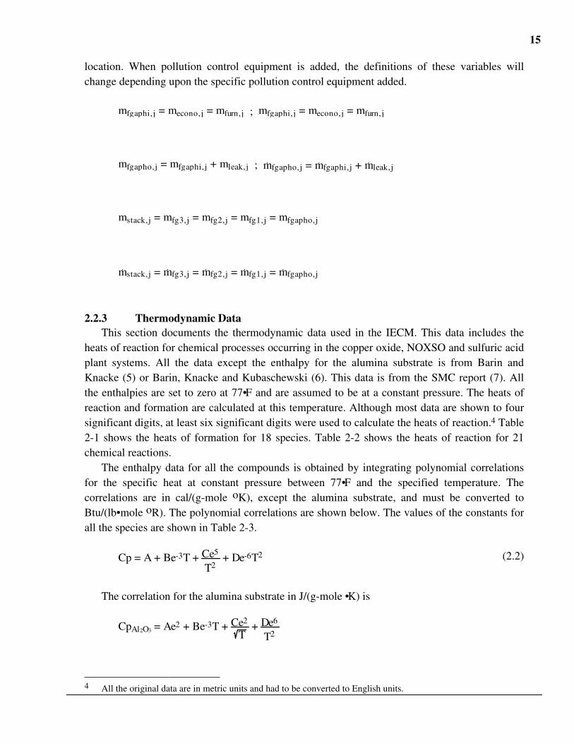
location. When pollution control equipment is added, the definitions of these variables willchange depending upon the specific pollution control equipment added.
mfgaphi,j = mecono,j = mfurn,j
;
mfgaphi,j = mecono,j = mfurn,j
mfgapho,j = mfgaphi,j + mleak,j
;
mfgapho,j = mfgaphi,j + mleak,j
mstack,j = mfg3,j = mfg2,j = mfg1,j = mfgapho,j
mstack,j = mfg3,j = mfg2,j = mfg1,j = mfgapho,j
2.2.3 Thermodynamic DataThis section documents the thermodynamic data used in the IECM. This data includes the
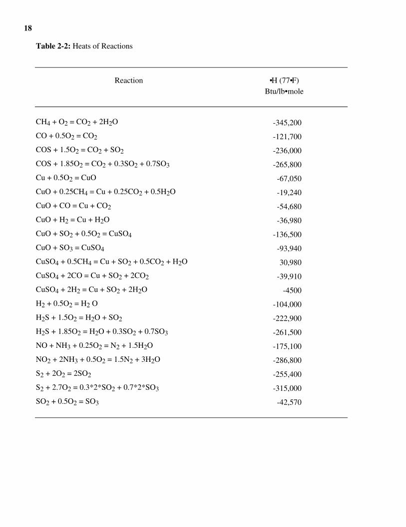
heats of reaction for chemical processes occurring in the copper oxide, NOXSO and sulfuric acidplant systems. All the data except the enthalpy for the alumina substrate is from Barin andKnacke (5) or Barin, Knacke and Kubaschewski (6). This data is from the SMC report (7). Allthe enthalpies are set to zero at 77•F and are assumed to be at a constant pressure. The heats ofreaction and formation are calculated at this temperature. Although most data are shown to foursignificant digits, at least six significant digits were used to calculate the heats of reaction.4 Table2-1 shows the heats of formation for 18 species. Table 2-2 shows the heats of reaction for 21chemical reactions.
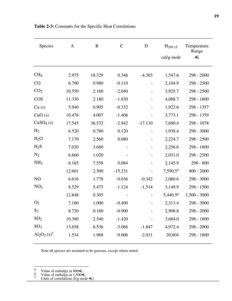
The enthalpy data for all the compounds is obtained by integrating polynomial correlationsfor the specific heat at constant pressure between 77•F and the specified temperature. Thecorrelations are in cal/(g-mole oK), except the alumina substrate, and must be converted toBtu/(lb•mole oR). The polynomial correlations are shown below. The values of the constants forall the species are shown in Table 2-3.
Cp = A + Be-3T + Ce5
T2 + De-6T2 (2.2)
The correlation for the alumina substrate in J/(g-mole •K) is
CpAl2O3 = Ae2 + Be-3T + Ce2
T + De6
T2
4 All the original data are in metric units and had to be converted to English units.
16
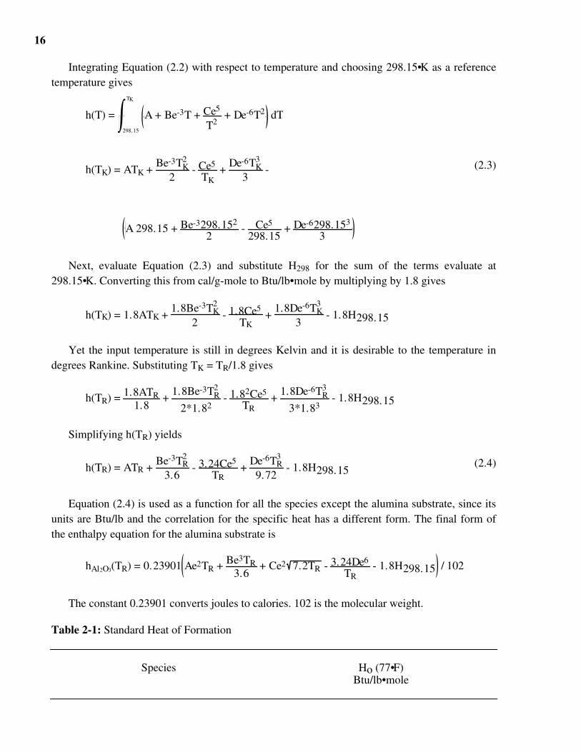
Integrating Equation (2.2) with respect to temperature and choosing 298.15•K as a referencetemperature gives
h(T) = A + Be-3T + Ce5
T2 + De-6T2 dT
298.15
TK
h(TK) = ATK + Be-3TK
2
2 - Ce5
TK +
De-6TK3
3 - (2.3)
A 298.15 + Be-3298.152
2 - Ce5
298.15 + De-6298.153
3
Next, evaluate Equation (2.3) and substitute H298 for the sum of the terms evaluate at298.15•K. Converting this from cal/g-mole to Btu/lb•mole by multiplying by 1.8 gives
h(TK) = 1.8ATK + 1.8Be-3TK
2
2 - 1.8Ce5
TK +
1.8De-6TK3
3 - 1.8H298.15
Yet the input temperature is still in degrees Kelvin and it is desirable to the temperature indegrees Rankine. Substituting TK = TR/1.8 gives
h(TR) = 1.8ATR1.8
+ 1.8Be-3TR
2
2*1.82 - 1.82Ce5
TR +
1.8De-6TR3
3*1.83 - 1.8H298.15
Simplifying h(TR) yields
h(TR) = ATR + Be-3TR
2
3.6 - 3.24Ce5
TR +
De-6TR3
9.72 - 1.8H298.15
(2.4)
Equation (2.4) is used as a function for all the species except the alumina substrate, since itsunits are Btu/lb and the correlation for the specific heat has a different form. The final form ofthe enthalpy equation for the alumina substrate is
hAl2O3(TR) = 0.23901 Ae2TR + Be3TR3.6
+ Ce2 7.2TR - 3.24De6
TR - 1.8H298.15 / 102
The constant 0.23901 converts joules to calories. 102 is the molecular weight.
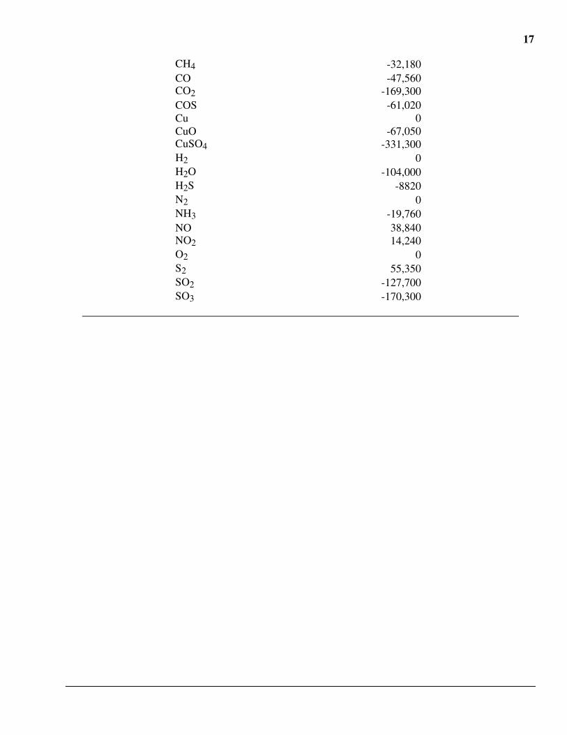
Table 2-1: Standard Heat of Formation
Species Ho (77•F)Btu/lb•mole
17
CH4 -32,180CO -47,560CO2 -169,300COS -61,020Cu 0CuO -67,050CuSO4 -331,300H2 0H2O -104,000H2S -8820N2 0NH3 -19,760NO 38,840NO2 14,240O2 0S2 55,350SO2 -127,700SO3 -170,300
18
Table 2-2: Heats of Reactions
Reaction •H (77•F)Btu/lb•mole
CH4 + O2 = CO2 + 2H2O -345,200
CO + 0.5O2 = CO2 -121,700
COS + 1.5O2 = CO2 + SO2 -236,000
COS + 1.85O2 = CO2 + 0.3SO2 + 0.7SO3 -265,800
Cu + 0.5O2 = CuO -67,050
CuO + 0.25CH4 = Cu + 0.25CO2 + 0.5H2O -19,240
CuO + CO = Cu + CO2 -54,680
CuO + H2 = Cu + H2O -36,980
CuO + SO2 + 0.5O2 = CuSO4 -136,500
CuO + SO3 = CuSO4 -93,940
CuSO4 + 0.5CH4 = Cu + SO2 + 0.5CO2 + H2O 30,980
CuSO4 + 2CO = Cu + SO2 + 2CO2 -39,910
CuSO4 + 2H2 = Cu + SO2 + 2H2O -4500
H2 + 0.5O2 = H2 O -104,000
H2S + 1.5O2 = H2O + SO2 -222,900
H2S + 1.85O2 = H2O + 0.3SO2 + 0.7SO3 -261,500
NO + NH3 + 0.25O2 = N2 + 1.5H2O -175,100
NO2 + 2NH3 + 0.5O2 = 1.5N2 + 3H2O -286,800
S2 + 2O2 = 2SO2 -255,400
S2 + 2.7O2 = 0.3*2*SO2 + 0.7*2*SO3 -315,000
SO2 + 0.5O2 = SO3 -42,570
19
Table 2-3: Constants for the Specific Heat Correlations
Species A B C D H298.15 TemperatureRange
cal/g-mole •K
CH4 2.975 18.329 0.346 -4.303 1,547.6 298 - 2000
CO 6.790 0.980 -0.110 - 2,104.9 298 - 2500
CO2 10.550 2.160 -2.040 - 3,925.7 298 - 2500
COS 11.330 2.180 -1.830 - 4,088.7 298 - 1800
Cu (s) 5.940 0.905 -0.332 - 1,922.6 298 - 1357
CuO (s) 10.476 4.007 -1.406 - 3,773.1 298 - 1359
CuSO4 (s) 17.545 36.532 -2.942 -17.110 7,690.4 298 - 1078
H2 6.520 0.780 0.120 - 1,938.4 298 - 3000
H2O 7.170 2.560 0.080 - 2,224.7 298 - 2500
H2S 7.020 3.680 - - 2,256.6 298 - 1800
N2 6.660 1.020 - - 2,031.0 298 - 2500
NH3 6.165 7.558 0.084 - 2,145.9 298 - 800
12.601 2.500 -15.231 - 7,590.55 800 - 2000
NO 6.616 1.778 -0.036 -0.342 2,060.6 298 - 3000
NO2 8.529 5.475 -1.124 -1.514 3,149.9 298 - 1500
12.848 0.305 - - 5,440.56 1,500 - 3000
O2 7.160 1.000 -0.400 - 2,313.4 298 - 3000
S2 8.720 0.160 -0.900 - 2,908.8 298 - 2000
SO2 10.380 2.540 -1.420 - 3,684,0 298 - 1800
SO3 13.658 6.536 -3.086 -1.847 4,972.4 298 - 2000
Al2O3 (s)7 1.534 1.968 -9.006 -2.031 20,804 298 - 1800
Note all species are assumed to be gaseous, except where noted.
5 Value of enthalpy at 800•K.6 Value of enthalpy at 1,500•K.7 Units of correlations J/(g-mole •K)
20
2.3 Boiler Efficiency
This section describes the algorithm used to calculate the boiler efficiency. The boilerefficiency is determined for a power plant without any pollution control equipment. This fixesthe amount of fuel entering the furnace. Any changes in the energy efficiency of the boilercaused by pollution control equipment is considered by the energy credit algorithm. The airpreheater is described in more detail in the next section. Yet, it is necessary to understand that theair preheater is divided into an ideal heat exchanger (i.e., no leakage) followed by a sectionwhere air leaks into the flue gas (see Figure 2-2). The uncorrected air preheater temperature,Tunc,orig, is the flue gas temperature after the heat exchanger.
The boiler efficiency in the IECM is based on the algorithm in “Steam/ Its Generation andUse”, by Babcock and Wilcox (8) and “Combustion, Fossil Power Systems”, by CombustionEngineering, Inc (9). The boiler efficiency is the energy absorbed by the steam cycle divided bythe energy in the fuel. The energy that is not absorbed by the steam cycle is lost to theenvironment. These losses can be categorized into five areas:
• sensible heat loss of the dry flue gas• sensible and latent heat loss from water vapor• unburned carbon and carbon monoxide• radiation loss• unaccounted lossesTherefore, the boiler efficiency is
ηboiler = 1 - LGas - LH2O - LC - LR - LUnacc
The sensible heat loss of the dry flue gas is the energy that could be used if the dry flue gaswere cooled to the inlet air temperature of the air preheater, Tfdfan,orig. The inlet fuel temperatureis assumed to be the same as the combustion air. This energy loss in Btu per pound of fuel can bedefined as
SEGas = mfgaphi,j,orig hj(Tunc,orig) - hj(Tfdfan,orig)j = 1
8
where j equals all the flue gas components except H2OThis energy loss can be expressed as a fraction of the fuel’s energy content by dividing it by
the higher heating value.
LGas = SEGasHhv
The heat loss due to water vapor in the flue gas can be split into the latent heat ofvaporization and the sensible heat loss. The latent heat loss is the energy that could be used if thewater vapor in the flue gas was condensed. Every pound of water vapor that is condensedreleases 1,040 Btu of energy. The water vapor in the flue gas is produced by the vaporization of
21
moisture in the fuel and the combustion of hydrogen in the fuel. The latent heat loss can becalculated as follows:
LE = fH2O + 18.02fH2*1.01
1,040
The sensible heat loss due to water vapor is the energy that could be used if the water vaporcould be cooled to the inlet air temperature, Tfdfan,orig. This energy loss can be calculated asfollows:
SEH2O = mfgaphi,H2O,orig hH2O(Tunc,orig) - hH2O(Tfdfan,orig)
The total loss from moisture expressed as a fraction is the sum of the latent heat and sensibleheat losses divided by the higher heating value of the fuel.
LH2O = LE + SEH2O
Hhv
Since the fuel’s higher heating value is based on the complete oxidation of carbon to carbondioxide, the boiler efficiency has to account for energy loss from unburned carbon and carbonmonoxide. Pure carbon has a higher heating value of 14,100 Btu/lb. The energy lost per pound ofunburned carbon is 14,100 Btu. For every pound of carbon converted to carbon monoxide, 9755Btu of energy are lost. The total energy loss due to unburned carbon and carbon monoxide is
LC = 12.01*9,755mfgaphi,co + 14,100CUnburned / Hhv
The loss from radiation exchange with the surroundings is estimated based on Figure 27 inreference (8) and Figure 6-5 in reference (9). Modern utility boilers usually have four watercooled walls and range in output from 800 to 6,000 million Btu per hour. Therefore, this curvewas fitted to the following equation between 800 and 6,000 million Btu per hour:
LR = 0.0015 + 6000MWg HRsteam
There are other minor losses that are not determined in this algorithm. An example of one ofthese losses is the sensible heat loss from the ash exiting the boiler. Theses losses and othermiscellaneous tolerance errors are entered as an input parameter in LUnacc.
2.4 Air Preheater
This section describes the performance and economic algorithms for the air preheater. Figure2-2 shows a schematic the air preheater. The purpose of the air preheater is to heat thecombustion air entering the boiler by cooling the flue gas exiting the boiler. Typically, there is a
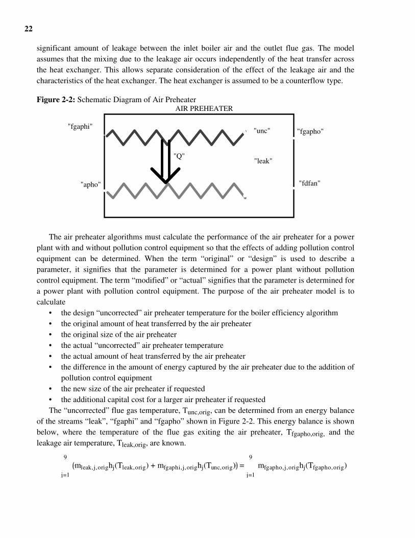
22
significant amount of leakage between the inlet boiler air and the outlet flue gas. The modelassumes that the mixing due to the leakage air occurs independently of the heat transfer acrossthe heat exchanger. This allows separate consideration of the effect of the leakage air and thecharacteristics of the heat exchanger. The heat exchanger is assumed to be a counterflow type.
Figure 2-2: Schematic Diagram of Air PreheaterAIR PREHEATER
"Q"
"fgaphi"
"apho" "fdfan"
"fgapho""unc"
"leak"
The air preheater algorithms must calculate the performance of the air preheater for a powerplant with and without pollution control equipment so that the effects of adding pollution controlequipment can be determined. When the term “original” or “design” is used to describe aparameter, it signifies that the parameter is determined for a power plant without pollutioncontrol equipment. The term “modified” or “actual” signifies that the parameter is determined fora power plant with pollution control equipment. The purpose of the air preheater model is tocalculate
• the design “uncorrected” air preheater temperature for the boiler efficiency algorithm• the original amount of heat transferred by the air preheater• the original size of the air preheater• the actual “uncorrected” air preheater temperature• the actual amount of heat transferred by the air preheater• the difference in the amount of energy captured by the air preheater due to the addition of
pollution control equipment• the new size of the air preheater if requested• the additional capital cost for a larger air preheater if requestedThe “uncorrected” flue gas temperature, Tunc,orig, can be determined from an energy balance
of the streams “leak”, “fgaphi” and “fgapho” shown in Figure 2-2. This energy balance is shownbelow, where the temperature of the flue gas exiting the air preheater, Tfgapho,orig, and theleakage air temperature, Tleak,orig, are known.
mleak,j,orighj(Tleak,orig) + mfgaphi,j,orighj(Tunc,orig)j=1
9
= mfgapho,j,orighj(Tfgapho,orig) j=1
9
23
Stream “fgapho” is equal to the sum of streams “leak” and “fgaphi”. Therefore, the energybalance can be rearranged as follows
mfgaphi,j,orig hj(Tunc,orig) - hj(Tfgapho,orig) = mleak,j,orig hj(Tfgapho,orig) - hj(Tleak,orig) j=1
9
j=1
9
The temperature difference between Tfgapho,orig and Tunc,orig is usually less than 40•F, so theleft hand side of this equation can be estimated by the average heat capacity times thetemperature difference between Tunc,orig and Tfgapho,orig. The average heat capacity is estimatedbetween Tfgapho,orig and Tfgapho,orig + 40•F. Therefore, Tunc,orig is determined by
Tunc,orig =
mleak,j,orig hj(Tfgapho,orig) - hj(Tleak,orig) j=1
9
Cpfgaphi,avg,orig + Tfgapho,orig
where
Cpunc,avg,orig =
mfgaphi,j,orig hj(Tfgapho,orig+40) - hj(Tfgapho,orig) j=1
9
40
The amount of energy transferred from the flue gas to the combustion air for a power plantwithout pollution control equipment is
Qaph,orig = 2000Mfuel mfgaphi,j,orig hj(Tfgaphi,orig) - hj(Tunc,orig)j=1
9
The temperature of the combustion air exiting the air preheater is typically less than 535•F. Itcan be estimated by
Tapho,orig =Qaph,orig
2000MfuelCpapho,avg,orig + Tfdfan,orig
where
Cpapho,avg,orig =
mapho,j,orig hj(985) - hj(Tfdfan,orig) j=1
9
985 - Tfdfan,orig
The size of the air preheater is estimated by the quantity UA, where U is the overall heattransfer coefficient and A is the surface area. For a given heat exchanger, the heat transfer can beestimated by the equation below, where the subscripts “i” and “o” represent “in” and “out” and“h” and “c” represent “hot” and “cold” respectively (10).
Q = UA Th,i - Tc,o - Th,o - Tc,i
lnTh,i - Tc,o
Th,o - Tc,i

24
Solving the above equation for UA for the original air preheater. Substituting the appropriatesubscripts yields
UAaph,orig =Qaph,orig
Tfgaphi,orig - Tapho,orig - Tunc,orig - Tfdfan,orig ln
Tfgaphi,orig - Tapho,orig
Tunc,orig - Tfdfan,orig(2.65)
Certain pollution control equipment, such as the copper oxide and NOXSO processes,significantly change the composition and temperature of the flue gas entering the air preheater.These changes may increase or decrease the amount of energy captured by the air preheater orchange the exit temperature of the flue gas exiting the air preheater. Two cases can beconsidered. The first (or base) case is using the original air preheater without modifications. Thealternative is to resize the air preheater so that additional energy can be captured by the airpreheater.
For the base case, the original air preheater is used so its size is fixed and the overall heattransfer coefficient is assumed to be constant. Therefore, the known values are
• flue gas flow rate, mfgaphi and inlet temperature, Tfgaphi
• combustion air flow rate, mapho and inlet temperature, Tfdfan,orig
• leakage air flow rate, mleak,orig and inlet temperature, Tleak,orig
• the product of the overall heat transfer coefficient and surface area, UAIt should be noted that mapho, mfgaphi and Tfgaphi are known, but their values may be
different from their value for the original power plant without pollution control equipment.The output parameters are the energy transferred across the air preheater, Qaph, the flue gas
exit temperature, Tfgapho, the “uncorrected” flue gas temperature, Tunc and the combustion airexit temperature, Tapho. To simplify the algorithms the average heat capacity of the flue gasentering the air preheater and the combustion air exiting the air preheater is determined.
Cpapho,avg =
mapho,j hj(Tfgaphi-100) - hj(Tfdfan,orig) j=1
9
Tfgaphi-100 - Tfdfan,orig
Cpfgaphi,avg =
mfgaphi,j hj(Tfgaphi) - hj(Tfgapho,input) j=1
9
Tfgaphi - Tfgapho,input
The variable Tfgapho,input is the new flue gas exit temperature when the air preheater isresized. It is used for the base case as a matter of convenience to determine the average heatcapacity of the flue gas. Once the average heat capacities are calculated, the “uncorrected” fluegas temperature, Tfgapho, is determined using the effectiveness-NTU method. The effectiveness,ε, is the ratio of the actual heat transfer rate for the heat exchanger to the maximum heat transferrate.
ε = Q
Qmax =
Cph(Th,i - Th,o)Cpmin(Th,i - Tc,i)
(2.5)
25
The subscript “min” indicates the stream with the lower heat capacity, while the subscript“max” indicates the stream with the higher heat capacity. For a counterflow heat exchanger withboth fluids unmixed, the effectiveness can approximated with the following relation.
ε = 1 - exp -NTU 1 -
Cpmin
Cpmax
1 - Cpmin
Cpmaxexp -NTU 1 -
Cpmin
Cpmax
(2.6)
In fossil fuel fired power plants, the hot fluid stream (flue gas) is significantly larger than thecold fluid stream. Therefore, the hot fluid stream has a greater heat capacity rate than the coldfluid. Equations (2.5) and (2.6) can be solved for Th,o by substituting Cc for Cmin and Ch forCmax and eliminating ε.
Th,o= Th,i - (Th,i - Tc,i)1 - exp -NTU 1 -
Cpmin
Cpmax
Cph
Cpc - exp -NTU 1 -
Cpmin
Cpmax
(2.7)
The number of transfer units (NTU) is a dimensionless parameter in heat exchanger analysisand is
NTU= UACpmin
Since UA is known, the term in the exponential of Equation (2.7) can be replaced by
d = - NTU 1 - Cpc
Cph = -UA
Cpc 1 -
Cpc
Cph = UA Cph
-1 - Cpc-1
Therefore, Equation (2.7) can be written as
Th,o= Th,i - (Th,i - Tc,i) 1 - ed
Cph
Cpc - ed
Substituting the appropriate subscripts for the air preheater into the above equations yields
Tunc= Tfgaphi - (Tfgaphi - Tfdfan) 1 - ed
Cpfgaphi,avg
Cpapho,avg - ed
d = UAaph,orig(Cpfgaphi,avg-1 - Cpapho,avg
-1 )
Once the “uncorrected” flue gas temperature is determined the flue gas and combustiontemperatures exiting the air preheater and the heat transfer across the air preheater can bedetermined.
26
Cpleak,avg =
mleak,j hj(Tunc) - hj(Tleak,orig) j=1
9
Tunc - Tleak,orig
Tfgapho = Cpleak,avgTleak,orig + Cpfgaphi,avgTunc
Cpleak,avg + Cpfgaphi,avg
Qaph = Cpfgaphi,avg(Tfgaphi - Tunc)
Tapho = Qaph
Cpapho,avg + Tfdfan,orig
For the resize case, the air preheater is resize so that the flue gas has an exit temperature ofTfgapho,input. Therefore, the known values are
• flue gas flow rate, mfgaphi and inlet temperature, Tfgaphi
• combustion air flow rate, mfgapho and inlet temperature, Tfdfan,orig
• leakage air flow rate, mleak,orig and inlet temperature, Tleak,orig
• the flue gas exit temperature, Tfgapho,input
The output parameters are the energy transferred across the air preheater, Qaph, the“uncorrected” flue gas temperature, Tfgapho and the combustion air exit temperature, Tfgapho andthe air preheater size, UA. Since Tfgapho,input is specified, the “uncorrected” flue gas temperatureis
Tunc =
mleak,j,orig(hj(Tfgapho,input) - hj(Tfgapho,input))j=1
9
Cpfgaphi,avg + Tfgapho,input
With the “uncorrected” flue gas temperature, the flue gas and combustion temperaturesexiting the air preheater and the heat transfer across the air preheater can be determined. The fluegas exit temperature, Tfgapho, should be very close to Tfgapho,input.
Tfgapho = Cpleak,avgTleak,orig + Cpfgaphi,avgTunc
Cpleak,avg + Cpfgaphi,avg
Qaph = Cpfgaphi,avg(Tfgaphi - Tunc)
Tapho = Qaph
Cpapho,avg + Tfdfan,orig
27
Once all the exit temperatures are determined, the new air preheater size, UAaph, can bedetermined with
UAaph =Qaph
Tfgaphi - Tapho - Tunc - Tfdfan,orig ln
Tfgaphi - Tapho
Tunc - Tfdfan,orig
Once the new size is determined, the additional capital cost in millions of current dollars canbe estimated by
Capaph = 2.6x10³(UAaph0.6 - UAaph,orig
0.6 ) CidxCidx,1984
For either the base case or the resize case, the difference in the energy transfer across the airpreheater can be determined by
Qaph,delta = Qaph - Qaph,orig
This difference in the energy transfer is an energy credit and how it affects the economics ofthe power plant is discussed in Section 2.7.
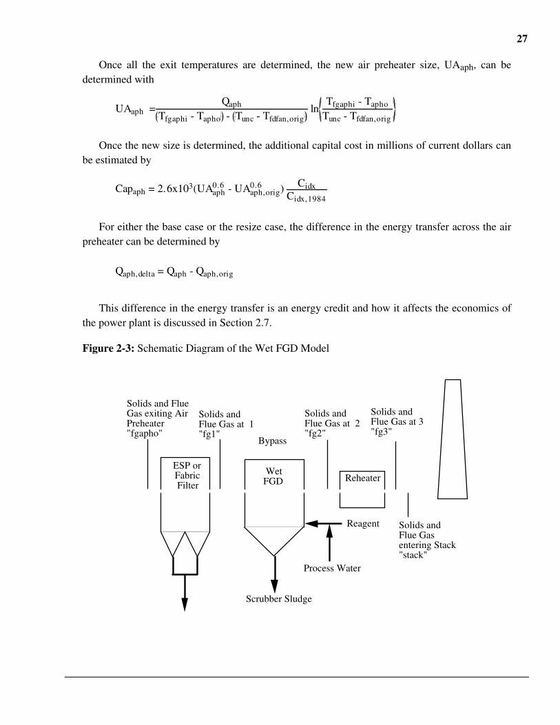
Figure 2-3: Schematic Diagram of the Wet FGD Model
ReheaterWet FGD
ESP or Fabric Filter
Bypass
Solids and Flue Gas exiting Air Preheater "fgapho"
Solids and Flue Gas at 1 "fg1"
Solids and Flue Gas at 2 "fg2"
Solids and Flue Gas at 3 "fg3"
Solids and Flue Gas entering Stack "stack"
Scrubber Sludge
Reagent
Process Water
28
2.5 Wet FGD Performance
This section describes the improvements to the wet flue gas desulfurization (FGD) modelsince the original model development (1). The quantities that were modified are the reagentcomposition, water evaporation in the scrubber, flue gas composition exiting scrubber, energyneeded for reheat, characterization of the scrubber waste and the capital cost when using lime asa reagent. A schematic diagram of the wet scrubber is shown in Figure 2-3. The diagram shows aconfiguration with bypass and a reheater. These options are mutually exclusive, since it is notlikely that a scrubber would be built with both. So, if there is a bypass, the reheater is not used.Conversely, if there is no bypass, the reheater is used to raise the flue gas temperature to aspecified value.
2.5.1 Reagent and SO2 EfficiencyThe SO2 removal efficiency is a key parameter governing the performance of the FGD
system. The removal efficiency can either be specified or it can be calculated to meet a desiredSO2 emission standard. The SO2 removal efficiency, ηSO2, based on the emission standard iscalculated by
ηSO2,std = 1 - 2000 ESSO2
Mfuel Hhvfuel
64.06 * 1,000,000 (min,SO2 + min,SO3
)
ηSO2,std = 1 - ESSO2
Mfuel Hhvfuel 64.06 * 500 (min,SO2
+ min,SO3)
(2.8)
The wet FGD system has an option to allow bypassing of some flue gas around the scrubber.This option may lower the cost of the wet FGD system if the efficiency calculated by Equation(2.8) is not very high. When the bypass option is chosen the scrubber operates at its maximumremoval efficiency, ηSO2,max, provided the amount of bypass is greater than the minimum bypassspecified by the user, Bypmin. Since the bypass does not affect the total amount of sulfurremoved, the moles of sulfur removed by the scrubber are determined from the Equation (2.8).
if 1 - ηSO2,std
ηSO2,max Bypmin then
Byp = 1 -
ηSO2,std
ηSO2,max ; ηSO2
= ηSO2,max
else Byp = 0.0 ; ηSO2 = ηSO2,std
mrem,S = ηSO2,std (min,SO2 + min,SO3)
The reagent for the wet scrubber can be either lime or limestone. The reagent purity, Rpurity
and moisture content, Wreag, must be specified. Any remaining material is considered inert. The
29
molar stoichiometry, σ, (moles of calcium required per mole of sulfur removed) must bespecified. The default values for the molar stoichiometry are 1.15 and 1.05 for limestone andlime, respectively. With the molar stoichiometry, the mass flow rate of reagent is calculated by
Mreag = 100.09 mrem,S σ
2000 Rpurity for CaCO3
;
Mreag = 56.08 mrem,S σ
2000 Rpurity for CaO
2.5.2 Water BalanceMakeup water to the FGD system is required principally to offset evaporative losses in the
scrubber. The mass of water evaporated in the FGD system is determined by an energy balanceassuming adiabatic conditions and neglecting the solid mass flow rates in the scrubber. Withthese assumptions, the sensible energy released by the flue gas entering the scrubber has to equalthe energy needed to evaporate the water evaporated and raise it to the exit temperature. Theequation for the energy balance is shown by Equation (2.9) for a scrubber without bypass8. Thefunction, Cp'in,avg is the average specific heat of the flue gas between the inlet temperature andthe Texit. The function, ∆h, is the energy needed to raise the makeup water to saturated steam atTexit.
Cp' in,avg(Tin,Texit) (Tin - Texit) min,jj=1
9
= Wevp ∆h(Texit) (2.9)
Tin = Tfg1 + ∆Tidfan
The temperature Tin is higher than Tin, since the induce draft fan raises the inlet temperatureby ∆Tidfan. The induced draft fan is assumed to be located between the scrubber and theparticulate collector. The flue gas is assumed to behave as an ideal mixture, so the molar fractionof water in the flue gas is equal to the parcel pressure of water divided by the total pressure of theflue gas. Since the flue gas is saturated when it exits the scrubber, the amount of waterevaporated is constrained by the saturation pressure of the water in the flue gas at the exittemperature. Since the change in the flue gas' total molar flow rate caused by the chemicalequations is very small, the water evaporation constraint is show in Equation (2.10).
Psat(Texit)Patm + Pg,exit
= Wevp + min,H2O
Wevp + min,jj=1
9
(2.10)
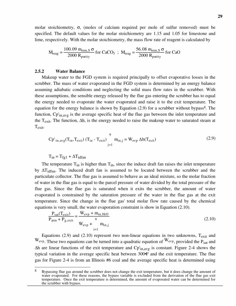
Equations (2.9) and (2.10) represent two non-linear equations in two unknowns, Texit andWevp. These two equations can be turned into a quadratic equation of Wevp, provided the Psat and∆h are linear functions of the exit temperature and Cp'in,avg is constant. Figure 2-4 shows thetypical variation in the average specific heat between 300•F and the exit temperature. The fluegas for Figure 2-4 is from an Illinois #6 coal and the average specific heat is determined using
8 Bypassing flue gas around the scrubber does not change the exit temperature, but it does change the amount of
water evaporated. For these reasons, the bypass variable is excluded from the derivation of the flue gas exittemperature. Once the exit temperature is determined, the amount of evaporated water can be determined forthe scrubber with bypass.
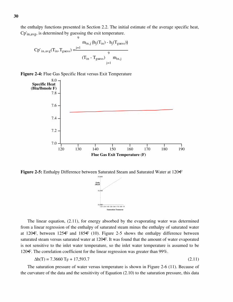
30
the enthalpy functions presented in Section 2.2. The initial estimate of the average specific heat,Cp'in,avg, is determined by guessing the exit temperature.
Cp' in,avg(Tin,Tguess) =
min,j hj(Tin) - hj(Tguess)j=1
9
(Tin - Tguess) min,jj=1
9
Figure 2-4: Flue Gas Specific Heat versus Exit Temperature8.0
7.8
7.6
7.4
7.2
7.0
190180170160150140130120Flue Gas Exit Temperature (F)
Specific Heat(Btu/lbmole F)
Figure 2-5: Enthalpy Difference between Saturated Steam and Saturated Water at 120•F
18,000
18,500
19,000
120 130 140 150 160 170 180 190
Saturation Temperatu
Entha(Btu/lb
The linear equation, (2.11), for energy absorbed by the evaporating water was determinedfrom a linear regression of the enthalpy of saturated steam minus the enthalpy of saturated waterat 120•F, between 125•F and 185•F (10). Figure 2-5 shows the enthalpy difference betweensaturated steam versus saturated water at 120•F. It was found that the amount of water evaporatedis not sensitive to the inlet water temperature, so the inlet water temperature is assumed to be120•F. The correlation coefficient for the linear regression was greater than 99%.
∆h(T) = 7.3660 TF + 17,593.7 (2.11)
The saturation pressure of water versus temperature is shown in Figure 2-6 (11). Because ofthe curvature of the data and the sensitivity of Equation (2.10) to the saturation pressure, this data
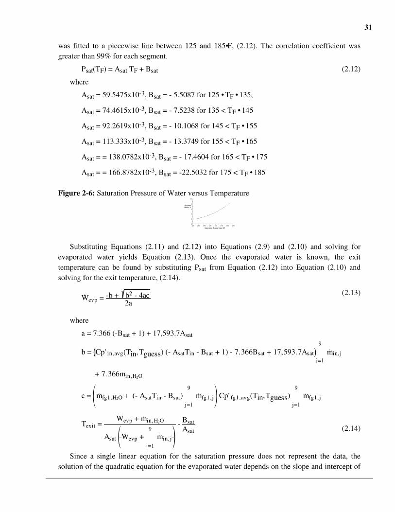
31
was fitted to a piecewise line between 125 and 185•F, (2.12). The correlation coefficient wasgreater than 99% for each segment.
Psat(TF) = Asat TF + Bsat (2.12)
where
Asat = 59.5475x10⁻³, Bsat = - 5.5087 for 125 • TF • 135,
Asat = 74.4615x10⁻³, Bsat = - 7.5238 for 135 < TF • 145
Asat = 92.2619x10⁻³, Bsat = - 10.1068 for 145 < TF • 155
Asat = 113.333x10⁻³, Bsat = - 13.3749 for 155 < TF • 165
Asat = = 138.0782x10⁻³, Bsat = - 17.4604 for 165 < TF • 175
Asat = = 166.8782x10⁻³, Bsat = -22.5032 for 175 < TF • 185
Figure 2-6: Saturation Pressure of Water versus Temperature
0
2
4
6
8
10
120 130 140 150 160 170 180 190
Pressure (lbf/in^2)
Saturation Temperature ÞF
Substituting Equations (2.11) and (2.12) into Equations (2.9) and (2.10) and solving forevaporated water yields Equation (2.13). Once the evaporated water is known, the exittemperature can be found by substituting Psat from Equation (2.12) into Equation (2.10) andsolving for the exit temperature, (2.14).
Wevp = -b + b2 - 4ac2a
(2.13)
where
a = 7.366 (-Bsat + 1) + 17,593.7Asat
b = Cp' in,avg(Tin,Tguess) (- AsatTin - Bsat + 1) - 7.366Bsat + 17,593.7Asat min,jj=1
9
+ 7.366min,H2O
c = mfg1,H2O + (- AsatTin - Bsat) mfg1,jj=1
9
Cp' fg1,avg(Tin,Tguess) mfg1,jj=1
9
Texit = Wevp + min,H2O
Asat Wevp + min,jj=1
9 - Bsat
Asat (2.14)
Since a single linear equation for the saturation pressure does not represent the data, thesolution of the quadratic equation for the evaporated water depends on the slope and intercept of
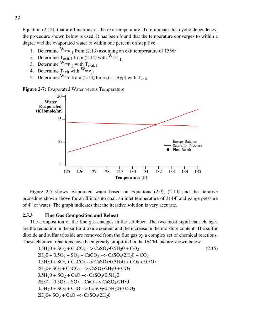
32
Equation (2.12), that are functions of the exit temperature. To eliminate this cyclic dependency,the procedure shown below is used. It has been found that the temperature converges to within adegree and the evaporated water to within one percent on step five.
1. Determine Wevp,1 from (2.13) assuming an exit temperature of 155•F
2. Determine Texit,1 from (2.14) with Wevp,1
3. Determine Wevp,2 with Texit,1
4. Determine Texit with Wevp,1
5. Determine Wevp from (2.13) times (1 - Byp) with Texit
Figure 2-7: Evaporated Water versus Temperature20
15
10
5
135134133132131130129128127126125Temperature (F)
WaterEvaporated
(K lbmole/hr)
Energy Balance Saturation Pressure Final Result
Figure 2-7 shows evaporated water based on Equations (2.9), (2.10) and the iterativeprocedure shown above for an Illinois #6 coal, an inlet temperature of 314•F and gauge pressureof 4” of water. The graph indicates that the iterative solution is very accurate.
2.5.3 Flue Gas Composition and ReheatThe composition of the flue gas changes in the scrubber. The two most significant changes
are the reduction in the sulfur dioxide content and the increase in the moisture content. The sulfurdioxide and sulfur trioxide are removed from the flue gas by a complex set of chemical reactions.These chemical reactions have been greatly simplified in the IECM and are shown below.
0.5H20 + SO2 + CaCO3 --> CaSO3•0.5H20 + CO2 (2.15)2H20 + 0.5O2 + SO2 + CaCO3 --> CaSO4•2H20 + CO2
0.5H20 + SO3 + CaCO3 --> CaSO3•0.5H20 + CO2 + 0.5O2
2H20+ SO3 + CaCO3 --> CaSO4•2H20 + CO2
0.5H20 + SO2 + CaO --> CaSO3•0.5H202H20 + 0.5O2 + SO2 + CaO --> CaSO4•2H200.5H20 + SO3 + CaO --> CaSO3•0.5H20+ 0.5O2
2H20+ SO3 + CaO --> CaSO4•2H20
33
Using these chemical reactions the composition of the flue gas exiting the scrubber can bedetermined from a molar balance and is shown below. It is assumed that the oxygen needed tooxidize the calcium sulfite to calcium sulfate is taken from the flue gas. In practice this oxygenmay be supplied by blowing air through the sludge outside the scrubber vessel. It is assumed thatthe water needed to hydrate the scrubber sludge comes directly from the makeup slurry and doesnot reduce the moisture content of the flue gas. The symbol Ox represents the fraction of calciumsulfite oxidized to calcium sulfate.
mexit,j = (1 - Byp) min,j for j = N2, CO, NO, NO2
mexit,O2 = (1 - Byp) min,O2 + 0.5(1 - Ox) min,SO3 - 0.5 Ox min,SO2 ηso2,std
mexit,H2O = (1 - Byp) min,H2O + Wevp
mexit,CO2 = (1 - Byp) min,CO2 + mrem,S if regent = CaCO3
mexit,SO2 = (1 - Byp) min,SO2 - min,SO2 ηSO2,std
mexit,SO3 = (1 - Byp) min,SO3
- min,SO3 ηSO2,std
The flue gas exiting the scrubber contains water droplets that the demister has not removed.These droplets evaporate either in the reheater or after the flue gas is remixed with the bypassedflue gas. These droplets are assumed to be a fraction, Wdemis, of the evaporated water:
mstack,j = mexit,j + Byp min,j for all j except H2O
mstack,H2O = mexit,H2O + Byp min,H2O + Wdemis Wevp
The flue gas exiting the scrubber is either remixed with the bypass flue gas or it passesthrough a reheater. Therefore, the flue gas temperature entering the stack is either the averagetemperature of the bypass flue gas and the flue gas exiting the scrubber or the exit temperature ofthe reheater. The exit temperature of the reheater is an input parameter, Tstack,input. The energyneeded to raise the flue gas temperature to Tstack is the sum of the sensible energy of the flue gasand the energy needed to evaporate the water droplets and raise their temperature to Tstack.
If no bypass then
Tstack = Tstack,input
34
Ewetfgd = Wdemis Wevp (7.366Tstack + 17593.7) + min,jj=1
9
hj(Tstack) - hj(Texit)
else
Tstack = Byp Tin + (1 - Byp) Texit
Ewetfgd = 0
2.5.4 Waste Stream CompositionA major environmental flow stream emanating from a wet FGD system is the stream of wet
solids. Two model options affect the mass flow rate of wet solids. The user specifies either aforced oxidation FGD system producing a gypsum waste or a natural oxidation FGD system thatproduces a wet sludge. The basic chemistry for these two options is shown in Equation (2.15).The difference in the composition and mass flow rates of FGD waste depends on the extent ofoxidation of calcium sulfite to sulfate, Ox and the extent of dewatering of the final product,Wsludge. Other constituents of the FGD solids stream include unreacted reagent (that depends onthe molar stoichiometry), inert materials introduced with the reagent (as dictated by the level ofreagent purity) and flyash that has been removed by the scrubber (that depends on the particulateremoval efficiency, ηTSP). The mass flow rates of the component are shown below.
Msludge,j = (1 - Byp) ηTSP Min,j for j = Ash, CaSO4
Msludge,CaO = (1 - Byp) ηTSP Min,CaO + 56.08 (σ - 1) mrem,S
2000 if reagent = CaO
Msludge,CaCO3 = (1 - Byp) ηTSP Min,CaCO3 + 100.09 (σ - 1) mrem,S
2000 if reagent = CaCO3
Msludge,CaSO3•0.5H2O = (1 - Byp) ηTSP Min,CaSO3•0.5H2O + 129.14 (1 - Ox) mrem,S
2000
Msludge,CaSO4•2H2O = (1 - Byp) ηTSP Min,CaSO4•2H2O + 172.17 Ox mrem,S
2000
Msludge,Misc = (1 - Byp) ηTSP Min,Misc + (1 - Rpurity - Wreag) Mreag
35
Msludge,H2O = 1Wsludge
- 1 Msludge,jj=1
8
for all j except H2O
2.5.5 Economics AlgorithmThe economic algorithm for the wet scrubber has remained unchanged except two items. The
first is that the single indirect charge factor originally employed for capital cost estimates hasbeen split into its component categories following the nomenclature used by the TennesseeValley Authority (TVA), author of the basic FGD cost model. The second change is in the directcapital cost for reagent handling. If lime is used as the reagent, the direct capital cost of reagenthandling is the same as the algorithm used for a spray dryer (1). If limestone is used, thealgorithm remains unchanged. The direct capital cost of reagent handling is shown below.
If Reagent = CaCO3
DCreag = If Mreag < 18 Then 0.1323 Mreag + 2.859 else 0.07288 Mreag + 5.393 CidxCidx,1981
else
DCreag = If Mreag < 2 Then 0.2997 Mreag + 1.546 else 0.1986 Mreag + 2.042 CidxCidx,1981
2.6 Spray Dryer Performance
This section describes improvements to the lime spray dryer performance model relative tothe previous report (1). The areas that were modified are the reagent composition, waterevaporation in the spray dryer, flue gas composition exiting spray dryer, energy needed for reheatand characterization of the scrubber waste. A schematic diagram of the spray dryer is shown inFigure 2-8. The diagram shows a configuration with bypass and a reheater. These options aremutually exclusive, since it is not likely that a spray dryer would be built with both. If there is abypass, the reheater is not used. Conversely, if there is no bypass, the reheater is used to raise theflue gas temperature to a specified value.
Figure 2-8: Schematic Diagram of the Spray Dryer FGD Model
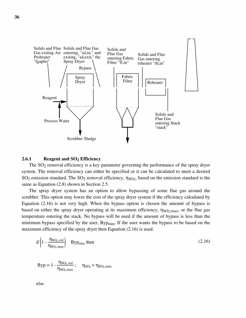
36
Spray Dryer Reheater
Fabric Filter
Bypass
Scrubber Sludge
Reagent
Process Water
Solids and Flue Gas exiting Air Preheater "fgapho"
Solids and Flue Gas entering Fabric Filter "ff,in"
Solids and Flue Gas entering reheater "rh,in"
Solids and Flue Gas entering Stack "stack"
Solids and Flue Gas entering, "sd,in," and exiting, "sd,exit," the Spray Dryer
2.6.1 Reagent and SO2 EfficiencyThe SO2 removal efficiency is a key parameter governing the performance of the spray dryer
system. The removal efficiency can either be specified or it can be calculated to meet a desiredSO2 emission standard. The SO2 removal efficiency, ηSO2, based on the emission standard is thesame as Equation (2.8) shown in Section 2.5.
The spray dryer system has an option to allow bypassing of some flue gas around thescrubber. This option may lower the cost of the spray dryer system if the efficiency calculated byEquation (2.16) is not very high. When the bypass option is chosen the amount of bypass isbased on either the spray dryer operating at its maximum efficiency, ηSO2,max, or the flue gastemperature entering the stack. No bypass will be used if the amount of bypass is less than theminimum bypass specified by the user, Bypmin. If the user wants the bypass to be based on themaximum efficiency of the spray dryer then Equation (2.16) is used.
if 1 - ηSO2,std
ηSO2,max Bypmin then (2.16)
Byp = 1 - ηSO2,std
ηSO2,max ; ηSO2
= ηSO2,max
else
37
Byp = 0.0 ; ηSO2 = ηSO2,std
The user may desire to have the bypass based on a desired stack temperature, Tstack,input.With this option, a bypass is only allowed if the bypass is greater than the minimum, Bypmin,and less than the amount determined by Equation (2.16). The induced draft fan is after the fabricfilter, (that is after the gases remix) and raises the temperature of the flue gas by a user specifiedamount, Tidfan. The flue gas exiting the spray dryer and the flue gas bypassed around the spraydryer are assumed to have the same specific heat; therefore, Equation (2.17) is used if the userwants the bypass to be based on the Tstack,input. The inlet temperature, Tin, equals thetemperature exiting the air preheater, Tfgapho, while the exit temperature, Texit, is determined inthe next section.
if Bypmin Š Tstack,input - Tidfan - Tsd,exit
Tfgapho - Tsd,exit Š 1 -
ηSO2,std
ηSO2,max then (2.17)
Byp = Tstack,input - Tidfan - Tsd,exit
Tfgapho - Tsd,exit ; ηSO2 =
ηSO2,std
1 - Byp
else
Byp = 0.0 ; ηSO2 = ηSO2,std
The flue gas that is not bypassed and the moles of sulfur removed by the scrubber aredetermined by
msd,in,j = (1 - Byp) mfgapho,j
mrem,S = ηSO2 (msd,in,SO2
+ msd,in,SO3)
The reagent for the spray dryer is lime. The reagent purity, Rpurity and moisture content,Wreag, must be specified. Any remaining material is considered inert. The molar stoichiometry,σ, (moles of calcium required per mole of sulfur into the system) is a function of the SO2
removal efficiency and the approach to saturation temperature (1). With the molar stoichiometry,the mass flow rate of reagent can be determined.
σsd = exp(3.322 ηSO2 + 0.025 ∆Tsat - 2.900) (2.18)
Mreag = 56.08 msd,in,SO2 + msd,in,SO3 σsd
2000 Rpurity(2.19)
38
2.6.2 Water BalanceMakeup water to the spray dryer system is required principally to offset evaporative losses in
the scrubber. The mass of water evaporated in the spray dryer system is determined by an energybalance assuming adiabatic conditions and neglecting the solid mass flow rates in the system.With these assumptions, the sensible energy released by the flue gas entering the scrubber has toequal the energy needed to evaporate the water evaporated and raise it to the exit temperature.This is identical with the wet scrubber, except that the flue gas exiting the spray dryer is notsaturated. The user specifies an approach to saturation temperature, ∆Tsat, which is a measure ofhow close the flue gas is to being saturated. The procedure for the spray dryer is identical withthe algorithm shown in Section 2.5, except steps 4 and 59. Once the saturation temperature, Tsat,of the flue gas is determined, the approach to saturation temperature is added to find the exittemperature. The evaporated water is determined with Equation (2.20), shown below, as follows:
1. Determine Wevp,1 from (2.13) assuming an exit temperature of 155•F
2. Determine Tsat,1 from (2.14) with Wevp,1
3. Determine Wevp,2 with Texit,1
4. Determine Tsat with Wevp,1, then Texit = Tsat + ∆Tsat.
5. Determine Wevp from (2.20)10
Wevp =
(1 - Byp) msd,in,j hj(Tfgapho) - hj(Tsd,exit)j=1
9
7.366 Tsd,exit + 17,593.7
(2.20)
2.6.3 Flue Gas Composition and ReheatThe composition of the flue gas changes in the spray dryer. The two most significant changes
are the reduction in the sulfur dioxide content and the increase in the moisture content. The sulfurdioxide and sulfur trioxide are removed from the flue gas by a complex set of chemical reactions.These chemical reactions have been greatly simplified in the IECM and are shown below:
SO2 + CaO + 0.5H20 --> CaSO3•0.5H20 (2.21)SO2 + CaO + 2H20 + 0.5O2 --> CaSO4•2H20SO3 + CaO + 0.5H20 --> CaSO3•0.5H20+ 0.5O2
SO3 + CaO + 2H20 --> CaSO4•2H20Using these chemical reactions the composition of the flue gas exiting the scrubber can be
determined from a molar balance and is shown below. It is assumed that the oxygen needed tooxidize the calcium sulfite to calcium sulfate is taken from the flue gas. In practice this oxygenmay be supplied by blowing air through the sludge outside the scrubber vessel. It is assumed thatthe water needed to hydrate the scrubber sludge comes directly from the makeup slurry and doesnot reduce the moisture content of the flue gas. The symbol Ox represents the fraction of calciumsulfite oxidized to calcium sulfate.
9 An additional assumption is needed for the spray dryer which is that the enthalpy of the water in the flue gas is
approximately equal to the enthalpy of saturated steam at the same temperature.10 Bypassing flue gas around the scrubber does not change the exit temperature, but it does change the amount of
water evaporated. For these reasons, the bypass variable is excluded from the derivation of the flue gas exittemperature. Once the exit temperature is determined, the amount of evaporated water can be determined forthe spray dryer with bypass.
39
msd,exit,j = msd,in,j for j = N2, CO2, CO, NO, NO2
msd,exit,O2 = msd,in,O2 + 0.5(1 - Ox) msd,in,SO3 - 0.5 Ox msd,in,SO2 ηSO2
msd,exit,H2O = msd,in,H2O + Wevp
msd,exit,SO2 = msd,in,SO2 - msd,in,SO2 ηSO2
msd,exit,SO3 = msd,in,SO3
- msd,in,SO3 ηSO2
After the spray dryer there are two options depending if a bypass is used. The first is that theflue gas is remixed with the bypassed flue gas before going into the fabric filter. After the fabricfilter the flue gas temperature is raised by the induced draft fan before entering the stack. Thesecond is that the flue gas passes through the fabric filter and induced draft fan before going intothe reheater. After exiting the reheater the flue gas enters the stack. For either case, the flue gascomposition and temperature do not change in the fabric filter. The equations governing the fluegas temperature and composition for the bypass case are shown below.
mff,in,j = msd,exit, j + Byp mfgapho,j
(2.22)
Tff,in = Byp Tfgapho + (1 - Byp) Tsd,exit (2.23)
mstack,in,j = mff,in,j(2.24)
Tstack = Tff,in + ∆Tidfan (2.25)
Edryfgd = 0 (2.26)
The equations governing the flue gas temperature and composition for the reheater case areshown below. The exit temperature of the reheater is an input parameter, Tstack,input. The energyneeded to raise the flue gas temperature to Tstack is the sensible energy of the flue gas.
mstack,in,j = mff,in,jmstack,j = mrh,in,j = mff,in,j = msd,exit,j(2.27)
Tff,in = Tsd,exit (2.28)
Trh,in = Tff,in + ∆Tidfan (2.29)
Tstack = Tstack,input (2.30)
40
Edryfgd = mrh,in,jj=1
9
hj(Tstack) - hj(Trh,in) (2.31)
2.6.4 Waste Stream CompositionA major environmental flow stream emanating from a spray dryer system is the stream of dry
waste solids. The basic chemistry for the creation of these solids is shown in Equation (2.21).The difference in the composition and mass flow rates of spray dryer waste depends on the extentof oxidation of calcium sulfite to sulfate, Ox. Other constituents of the spray dryer solids streaminclude unreacted reagent (that depends on the molar stoichiometry), inert materials introducedwith the reagent (as dictated by the level of reagent purity) and flyash. The total mass flow rate ofthe solids created in the spray dryer and the flyash entering the spray dryer is shown below.
Msd,total,j = Msd,in,j for j = Ash, CaCO3, CaSO4
Msd,total,CaO = Msd,in,CaO + 56.08 σ msd,in,SO2 + msd,in,SO3 - mrem,S
2000
Msd,total,CaSO3•0.5H2O = Msd,in,CaSO3•0.5H2O + 129.14 (1 - Ox) mrem,S
2000
Msd,total,CaSO4•2H2O = Msd,in,CaSO4•2H2O + 172.17 Ox mrem,S
2000
Msd,total,Misc = Msd,in,Misc + (1 - Rpurity - Wreag) Mreag
The total solids in the spray dryer either exit with the flue gas or drop out the bottom of thespray dryer. The removal efficiency, ηTSP, of the solids is an input parameter, that specifies whatfraction of the total solids exit out the bottom. The solids that exit with the flue gas remix withthe flyash bypassed around the spray dryer (if present) before entering the fabric filter. After thefabric filter removes most of the solids, the solids from the spray dryer and fabric filter areremixed before being disposed.
Msd,bottom,j = ηTSP Msd,total,j
41
Msd,exit,j = (1 - ηTSP) Msd,total,j
Mff,in,j = Byp Mfgapho,j + Msd,exit,j
2.6.5 Economics AlgorithmThe economic algorithm for the spray dryer has remained unchanged except one item. The
single indirect charge factor for capital cost has been split into different categories of indirectcharges following the nomenclature of the TVA.
2.7 Power Plant Economics
This section describes the economics of the base (original) power plant. Subsequent sectionsthen describe how the pollution control equipment affects the economics of the base plant. Thefollowing section will describe how the economics changes when pollution control equipment isadded. For purposes of cost estimate and internal consistency, the IECM effectively considers thepower plant and pollution control equipment to be separate entities. The base power plantessentially consumes fuel and produces electricity and flue gas, while the pollution controlequipment consumes some electricity and removes the pollutants from the flue gas.
2.7.1 Base Plant CostsThe base power plant uses electricity and steam for running pulverizers, steam cycle pumps,
flue gas fans, cooling system and miscellaneous other equipment. These components representinternal utility (auxiliary power) consumption that reduces the amount of electricity that thepower plant can sell to customers (including the pollution control equipment). The auxiliarypower consumption reduces the electricity available for sale and increases the heat rate.
MWbp = MWg 1 - xp - xsp - xf - xc - xmisc
HRbp = HRcycle
1 - xp - xsp - xf - xc - xmisc
The capital and operating cost of a power plant is based on the algorithms presented inMolberg (11). The direct and total capital costs are estimated as follows:
TDCbp = 600MWbp
1,000,000
0.85 HWidxHWidx,1988
42
TCCbp = TDCbp (1 + ICF)
The operating cost is divided into two categories: fuel cost and non-fuel cost. The non-fuelexpenses include labor, maintenance, overhead, taxes, etc… The fuel cost depends on the fuelconsumption and cost of fuel, while the non-fuel cost is proportional to the size of the powerplant.
ACfuel = 8766x10-6 CfmfuelPfuel
ACnon = 8766x10-6 Cf 4.35 MWbp CidxCidx,1988
ACbp = ACfuel + ACnon
The total revenue requirement excluding any income from “selling” electricity to thepollution control equipment can be calculated by annualizing the total capital cost and levelizingthe total operating and maintenance costs. The model does not explicitly charge the power plantfor its own utility consumption. The main reason is that any charge to the power plant iscollected by the power plant, so the net effect is zero. The price of electricity, Ecost, charged tothe pollution control equipment can be set to any value by the model user (as is typically done inmost economic analyses). However, the default is to use the marginal electricity cost based onthe total revenue requirement of the base plant without utilities:
TRRw/o util,bp = TCCbpFCF + ACbpVCLF(2.32)
Ecost = TRRw/o util,bpx106
8766CfMWbp
(2.33)
where 8766 is the average number of hours in a year (including leap years).
2.7.2 Pollution Control Equipment Energy PenaltiesThis section gives a brief overview of the economics of pollution control equipment and
describes in detail how the pollution control equipment affects the economics of the base powerplant. This section assumes that the pollution control equipment is a consumer of energy. Thenext section describes the effects when pollution control equipment contributes energy (e.g. fromexothermic chemical reactions). How the capital and operating costs of specific pollution controlequipment are determined is described in other chapters and is not covered in this section. Oncethe total capital and operating costs are determined for a specific pollution control equipment thetotal revenue requirement can be calculated.
43
TRRw/o util,pce,j = TCCpce,jFCF + ACpce,jVCLF
However, this does not reflect the cost of electricity and steam consumption charged to thepollution control equipment by the power plant. The utility cost is the equivalent electricityconsumption times the cost of electricity. Given the utility cost, the total revenue requirementcan be determined. This total revenue requirement can be expressed in mills per kilowatt hour bydivided it by the net electric capacity of the power plant.
ACutil,pce,j = 8766Cf MWbp xpce,j Ecost
TRRpce,j = TRRw/o util,pce,j + ACutil,pce,j
Epce,j = TRRpce,jx106
8766CfMWnet
The electricity consumption of the pollution control equipment reduces the amount ofelectricity available for sale to external customers. Therefore, the net electric capacity is the grosscapacity minus the internal consumption, including all pollution control equipment:
MWnet = MWg 1 - xp - xsp - xf - xc - xmisc - xpce,jj=1
n
Since the pollution control equipment “pays” the base power plant for electricityconsumption, these charges are income for the base power plant. The pollution controlequipment utility costs appear as negative charges (i.e. income) in the base power plant utilitycost. This procedure is a bookkeeping operation to change pollution control equipment for utilityuse:
ACutil,bp = - ACutil,pce,jj=1
n
The total revenue requirement including utility cost for the power plant can be calculated asthe sum of the total revenue requirement without utilities plus the utility cost for the base powerplant. The total revenue requirement can be divided by the net capacity to determine the cost ofelectricity including utility costs of the base power plant, Ebp. This cost of electricity, Ebp, willequal the price of electricity charged to the pollution control equipment, Ecost, if the pricecharged to the pollution control equipment is equal to the value determined by Equation (2.33).
TRRbp = TRRw/o util,bp + ACutil,bp(2.34)
44
Ebp = TRRbpx106
8766CfMWnet
(2.35)
2.7.3 Pollution Control Equipment Energy CreditsThis section describes the changes in economics when pollution control equipment
contributes energy that can be converted to electricity (as is true of an exothermic process thatincreases the potential heat input to the boiler). There are a variety of ways to treat this case. Forthe IECM, the pollution control equipment is assumed to sell the energy back to the power plant,that converts the additional energy into electricity for sale. Therefore, the revenue generated fromthe sale of energy to the power plant shows up as a credit in the operating costs for the pollutioncontrol equipment and a debit in the fuel cost of the power plant.
The power plant is considered to have two choices for treating this energy. Either it canreduce the amount of purchased fuel while the gross amount of electricity remains constant or itcan “build” additional equipment to convert this energy into additional electricity (i.e., increasethe gross plant size). The first choice requires an iterative solution since the energy generated bythe pollution control equipment is a function of the fuel consumption of the power plant.11
Because of the complexities of the IECM, it is not possible to solve this iterative problemexplicitly.
Instead, the IECM assumes the power plant builds additional equipment to convert theadditional energy into electricity. Since the IECM models new power plants, the additionalequipment is “built” simultaneously with the base power plant, yet is accounted separately in theeconomics. This approach allows a simpler solution. Or, the user simply can neglect the changein size since it is generally small and does not change the economics substantially. The additionalequipment has capital and non-fuel operating costs, that are charged to the base power plant.
The equivalent electric capacity of this energy is needed to determine the charges and debitsfor energy generated by pollution control equipment. If the additional energy is in the form ofheat captured by the air preheater, it is treated the same as the energy from coal. The additionalenergy is divided by the original heat rate. If the additional energy is in the form of steam, it istreated the same as energy in the steam cycle, so the additional energy is divided by the originalheat rate times the boiler efficiency. With the equivalent electric capacity, the electric capacity ofthe power plant with and without pollution control equipment also can be determined.
MWcredit = Qaph,delta
HRorig +
Qsteam
ηboilerHRorig
11 The energy generated by the pollution control equipment is based on the fuel flow rate into the power plant and
the characteristics of the specific pollution control equipment. So reducing the fuel flow rate into the powerplant, changes the energy generated by the pollution control equipment, which changes the fuel flow rate. Toaccurately solve this problem requires an interactive solution, since it is not possible to a priori determine theappropriate fuel flow rate and energy from the pollution control equipment to produce a specific amount ofelectricity.
45
MWbp,new = MWg 1 - xp - xsp - xf - xc - xmisc + MWcredit
MWnet = MWg 1 - xp - xsp - xf - xc - xmisc - xpce,jj=1
n
+ MWcredit
Multiplying the electric capacity by the heat rate and dividing by the higher heating value ofthe fuel gives the equivalent fuel consumption. The equivalent fuel consumption is multiplied bythe cost of fuel to determine the revenue from the sale of the energy to the power plant. Thisrevenue is credited to the operating cost of the pollution control equipment that generated theenergy.
mfuel,credit = MWcredit HRbp
2Hhv
ACfuel,credit = 8766x10-6 Cfmfuel,creditPfuel
ACpce,j = ACw/o credit,pce,j + ACfuel,credit
Several base plant economic variables must be modified to account for the energy credit. Thedirect capital cost for the additional equipment is estimated to be proportional to the direct capitalcost of the original power plant. Therefore, the direct capital cost is determined by
TDCbp = 600 1 + MWcreditMWbp
MWbp
1,000,000
0.85 HWidxHWidx,1988
The non-fuel operating and maintenance costs are estimated to be proportional to the non-fuel operating and maintenance cost of the original power plant. The total operating cost for thebase plant is
ACnon = 8766x10-6 Cf 4.35 MWbp + MWcredit Cidx
Cidx,1988
ACbp = ACfuel + ACnon + ACfuel,credit
46
The equations for the total revenue requirement, (2.34) and (2.32) and the cost of electricityof the base power plant, (2.35), do not change, but the equation for the default price of electricitycharged to pollution control equipment, (2.33), does change:
Ecost = TRRw/o util,bpx106
8766CfMWbp,new
2.7.4 Total Pollution Control CostThe total capital, operating, utility and revenue requirements for pollution control excluding
coal cleaning can be determined by summing the values the pollution control equipment:
TCCtotal,pce = TCCpce,jj=1
n
;
ACtotal,pce = ACpce,jj=1
n
TRRw/o util, total,pce = TRRw/o util,pce,jj=1
n
;
ACutil,total,pce = ACutil,pce,jj=1
n
TRRtotal,pce = TRRpce,jj=1
n
;
Etotal,pce = Epce,jj=1
n
The total capital, operating, utility and revenue requirements of the power plant are the sumof the base power plant and the total pollution control equipment.
TCCtotal = TCCbp + TCCtotal,pce
ACtotal = ACbp + ACtotal,pce
TRRw/o util,total = TCCw/o util,bp + TCCw/o util,total,pce
ACutil,total = ACutil,bp + ACutil,total,pce
TRRtotal = TCCbp + TCCtotal,pce
ECtotal = ECbp + ECtotal,pce
The total cost for pollution control including coal cleaning has to be determined byexamining two identical power plant. One power plant uses cleaned coal, while the other doesnot. The total pollution control costs are calculated by subtracting the base plant costs for theplant that is not using cleaned coal from the total plant costs for the plant that is using cleanedcoal. This procedure is necessary since the coal cleaning plant is assumed to be separate from thepower plant. The capital and operating costs of the coal cleaning plant are added to the cost ofraw coal, so delivered cost of coal to the power plant increases.
TCCtotal,pce = TCCtotal - TCCbp,w/o cc
ACtotal,pce = ACtotal - ACbp,w/o cc
47
TRRw/o util,total,pce = TCCw/o util,total - TCCw/o util,bp,w/o cc
ACutil,total,pce = ACutil,total - ACutil,bp,w/o cc
TRRtotal,pce = TCCtotal - TCCbp,w/o cc
ECtotal,pce = ECtotal - ECbp,w/o cc
2.8 Key Financial Parameters
2.8.1 Fixed Charge FactorThe fixed charge factor is used to convert the future carrying charges of the plant investment
into a uniform series of payments over the plant life. It is calculated based on the revenuerequirement methodology presented in the EPRI Technical Assessment Guide (12, 13).
Revenue requirements consist of two main components, carrying charges (fixed charges) andexpenses (operating costs). Carrying charges are related to the capital investment and areincurred despite how the plant is used. They consist of return on investment, book depreciation,income taxes, local property taxes and insurance. Expenses are related to the operation andmaintenance of the plant and generally used within one year and generally consist of fuel,operating and maintenance costs.
Book depreciation is the annual charge to repay the original investment. A straight linemethod is used in the IECM and it is assumed that the salvage value is equal to the cost ofretiring the plant. The current tax laws allow for an investment tax credit. This credit is animmediate reduction in the income taxes for the year that the plant goes into services. Theinvestment tax credit is normalized as opposed to “flow through” (these terms are explainedlater). Therefore, the book depreciation calculation is
Db = 1 - itcBl
Money to cover the total capital investment comes from the sale of bonds (known as debtfinancing) and the sale of common and preferred stock (equity financing). The ratio of debtfinancing to equity financing is generally around 50%. The return on debt and equity is themoney a utility must pay to its investors for using their money. The weighted average of thereturn on debt and equity is often called the “return on investment”, “cost of money” or the“weighted cost of capital”. This return is based on the undepreciated investment or the remainingbalance on the initial investment, that will be defined later in Equation (2.42). The annual rate ofreturn on debt and equity is related to the inflation rate. The IECM assumes that the real rate ofreturn or the return in the absence of inflation remains constant. Therefore, the rates of return areinput parameters expressed in constant dollars and the nominal or current rates of returns arecalculated with Equations (2.36), (2.37), (2.38). The weighted cost equity is shown in Equation(2.39), while the weighted cost of capital is shown in Equation (2.40).
B = (1 + ei) (1 + Br) - 1 (2.36)
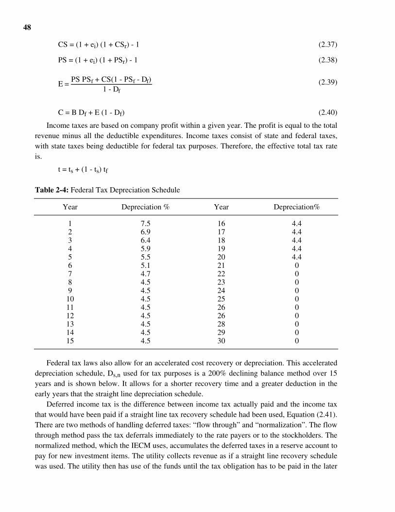
48
CS = (1 + ei) (1 + CSr) - 1 (2.37)
PS = (1 + ei) (1 + PSr) - 1 (2.38)
E = PS PSf + CS(1 - PSf - Df)
1 - Df
(2.39)
C = B Df + E (1 - Df) (2.40)
Income taxes are based on company profit within a given year. The profit is equal to the totalrevenue minus all the deductible expenditures. Income taxes consist of state and federal taxes,with state taxes being deductible for federal tax purposes. Therefore, the effective total tax rateis.
t = ts + (1 - ts) tf
Table 2-4: Federal Tax Depreciation Schedule
Year Depreciation % Year Depreciation%
1 7.5 16 4.42 6.9 17 4.43 6.4 18 4.44 5.9 19 4.45 5.5 20 4.46 5.1 21 07 4.7 22 08 4.5 23 09 4.5 24 010 4.5 25 011 4.5 26 012 4.5 26 013 4.5 28 014 4.5 29 015 4.5 30 0
Federal tax laws also allow for an accelerated cost recovery or depreciation. This accelerateddepreciation schedule, Ds,n used for tax purposes is a 200% declining balance method over 15years and is shown below. It allows for a shorter recovery time and a greater deduction in theearly years that the straight line depreciation schedule.
Deferred income tax is the difference between income tax actually paid and the income taxthat would have been paid if a straight line tax recovery schedule had been used, Equation (2.41).There are two methods of handling deferred taxes: “flow through” and “normalization”. The flowthrough method pass the tax deferrals immediately to the rate payers or to the stockholders. Thenormalized method, which the IECM uses, accumulates the deferred taxes in a reserve account topay for new investment items. The utility collects revenue as if a straight line recovery schedulewas used. The utility then has use of the funds until the tax obligation has to be paid in the later
49
years of the booklife. The deferred income taxes and the investment tax credit are called taxpreferences.
td,n = (Ds,n - 1/Bl) t for n = 1, Bl (2.41)
As mentioned earlier, the return on investment was based on the remaining balance. Theremaining balance per year is the initial investment minus the book depreciation, deferredincome tax per year and investment tax credit in the first year, Equation (2.42). The returns ondebt and equity per year are shown in Equation (2.43) and (2.44). The taxes paid per year areshown in Equation (2.45). The year by year carrying charges is just the sum of the bookdepreciation, deferred taxes, return on debt, return on equity, income taxes paid and theadvalorem tax, Equation (2.46).
RBn = RBn-1 - Db - td,n-1 (2.42)
RDn = RBn Df B (2.43)
REn = RBn (1 - Df) E (2.44)
tp,n = t1 - t
(Db - Ds,n + td,n + REn) (2.45)
CCn = Db + td,n + RDn + REn + tp,n + a for n = 1,Bl (2.46)
RB1 = 1 - itc
The discount rate used for present value calculations is related to the weighted cost of capital.The most common method used in the utility industry is a “before tax discount rate” that is equalto the weighted cost of capital. Some industries use an “after tax discount rate” that is equal tothe weighted cost of capital less the tax rate times the return on debt. The IECM uses a “beforetax discount rate”, Equation (2.47). The present value factor of a future expense in a given year isgiven by Equation (2.48). It is assumed for present value calculations that all expenses are paid atthe end of year. The annuity factor shown in Equation (2.49), calculates the present value of auniform series of payments in the future, while the reciprocal of the annuity factor calculates anequivalent uniform annual amount for a single payment.
dis = C (2.47)
PVn = (1 + dis)n (2.48)
An = 1 - PVndis
(2.49)
The present value of future carrying charges is the sum of carrying charges times the presentvalue factor, Equation (2.50). The levelized carrying charge converts the actual carrying chargesthat vary from year to year into a uniform payment for the tax life of the plant. The levelizedcarrying charge per year is just the cumulative present value of the carrying charge divided by
50
the annuity, Equation (2.51). The levelized carrying charge for the last year of the book life is thefixed charge factor, Equation (2.52).
CCpv,n = CCm PVmm=1
n
(2.50)
CCl,n = CCpv,n
An (2.51)
FCF = CCl,Bl (2.52)
2.8.2 Levelization FactorThe levelization algorithm is used to convert a series of future payments that have a uniform
escalation rate into a uniform series of payments over the same period. The IECM assumes thatthe real escalation rate for expenses is constant, so the apparent escalation rate is calculated fromEquation (2.53). The levelization factor is calculated with Equation (2.54). The total revenuerequirement is calculated in Equation (2.55).
ef = (1 + er) (1 + ei) - 1 (2.53)
Ln = k (1 - kn)ABl(1 - k)
where k = 1 + ef1 + dis
(2.54)
TRR = TCC FCF + TVC LBl (2.55)
2.8.3 Year-by-Year Revenue Requirement AnalysisA year-by-year revenue requirement analysis is also available in the IECM. This method has
the advantage of showing the revenue requirement in current dollars over the entire tax life. Thetotal revenue requirement in a future year is the sum of the carrying charges and the operatingexpenses.
TCCn = TCC CC
TVCn = TVC (1 + ef)n
TRRn = TCCn + TVCn
2.8.4 Accumulated Funds Used During ConstructionThe accumulated funds used during construction, AFUDC, or interest during construction is
determined from the total plant cost, TPC. It is assumed that the equipment begins service at thebeginning of January and that the construction takes place during the preceding years. Also theIECM determines the total plant cost in the same year dollars that the equipment begins services.The actual cashed expended for construction is assumed to be spent uniformly at the middle of
51
each year during construction. Therefore, the total cash expended, TCE, in mixed year dollars, isfound by de-escalating the total plant cost back in time.
TCE = TPCN
11 + i j-0.5
j=1
N
After the money is spent, interest charges are accumulated as part of the AFUDC at adiscount rate, dis. The discount rate is determined from Equation (2.47). Therefore, the totalplant investment, TPI, is
TPI = TPCN
1 + dis j-0.5
1 + i j-0.5j=i
N
= TPCN
1 + dis1 + i
j-0.5
j=1
N
The AFUDC is the difference between the total plant investment and the total cash expended.
AFUDC = TPI - TCE
2.9 Conventional Coal Cleaning
2.9.1 IntroductionThis section describes the changes to the conventional coal cleaning model. A detailed
description of the conventional coal cleaning model is contained in Reference (1). Figures 2-9 -2-11 show the schematic diagrams for coal cleaning plants of levels 2, 3 and 4. The subscript “i”in this section refers to the coarse, medium or fine streams of the coal cleaning plant.
2.9.2 Level 4 Plant CostAfter reviewing the economics for a level four plant, several cost coefficients were modified
to more accurately represent level four plants that use hydrocyclones. These changes are minorand do not change the cost of cleaning a given coal significantly. The new cost coefficients weremodified for the direct capital cost, chemicals, electricity and water are:
DCC4 = 45,700
c4 = 0.065
e4 = 0.158
w4 = 0.0041
2.9.3 Moisture Content of Cleaned CoalAnother improvement to the coal cleaning model is that it now more accurately calculates the
moisture content of the cleaned and refuse coal. Previously the model did not explicitly calculatethe moisture content of the cleaned or refuse coal and it did not adjust the final quality of the coalto account for the thermal drier. These assumptions made the model less sensitive to the effectsof the different moisture content associated with different size wash streams.
The revised model assumes that the total moisture content of the raw coal is composed of twocomponents: the inherent moisture and the surface moisture. The inherent moisture is assumed to
52
remained constant even if the coal is washed or thermally dried. The surface moisture of the coalchanges if it is washed or thermally dried. The model requires that the surface moistureassociated with each wash stream be entered as an input parameter. The value should be typicalof the surface moisture associated with the wash size stream after it has been through mechanicaldewatering. In other words, as the wash stream size decreases the surface moisture shouldincrease. For example, 28x0 mesh coal would have a surface moisture of approximately 20%,while 1.375”x0.25” would have a value of approximately 4%.
The total moisture content of each wash stream is equal to the inherent moisture content ofthe raw coal plus the surface moisture of either the wash stream (if the stream was washed) or theraw coal Equation.
If Yi < 1 then
m'i =mi'ROM + ms'i
else
m'i =mi'ROM + ms'ROM
To calculate the average properties of the coal entering the thermal drier, the fraction of coalto be thermally dried needs to be determined. Equation (2.56) calculates the weight fraction ofthe coal exiting the washing equipment, while Equation (2.57) calculates the fraction of coal tobe thermally dried. The input parameter, δi, is used to determine which streams should bethermally dried. It is set to 1 if the stream is to be thermally dried; otherwise, it is 0. This allowsany combination of wash streams to be sent to the thermal drier.
fsc,i = fsROM,iYi
Yp(2.56)
fsd = fsc,iδii=1
3(2.57)
The surface moisture associated with a wash stream, ms'i, is an input parameter. Equations(2.58) and (2.59) show the equations for the average moisture content and higher heating value ofthe coal entering the thermal drier.
m' in =
m' ifsc,iδi
(1 - m' i)i=1
3
fsc,iδi
(1 - m' i)i=1
3 (2.58)
HHVd =
HHVifsc,iδii=1
3
fsd
(2.59)
53
The moisture content of the refuse streams is equal to the inherent moisture content of theraw coal plus surface moisture associated with the washed streams. Therefore, the averagemoisture content of the refuse coal is estimated with the equation below.
m' ref =
(mi' ROM + ms' i)(1 - Yi)fsROM,i
(1 - mi' ROM - ms' i)i=1
3
(1 - Yi)fsROM,i
(1 - mi' ROM - ms' i)i=1
3
With the moisture content and higher heating value of the coal entering the thermal drierdetermined, it is possible to calculate the performance of the thermal drier. Since the modelexplicitly calculates the moisture content of the coal entering the thermal drier, m'in, it is possiblefor that coal to be drier than the specified moisture content of the coal exiting the thermal drier,m'out. Thus, the thermal drier is used only if the coal entering the drier has a moisture contentabove a certain level. If the thermal drier is not used the thermal drier yield is set to 100 percentand the fraction of coal dried and water evaporated are set to zero. If it is used the fraction of coaldried is calculated with Equation (2.57) and the other parameters are calculated as follows.
m'out = mi'ROM + ms'out
If m'in < m'out then
w' = 0.0
Ed = 0.0
LHV = 0.0
Yd = 1.0
Yod = 1.0 (2.60)
w'e = 0.0
fsd = 0.0
δι = 0
else
w' = m' in - m' out(1 - m' in) (1 - m' out)
Ed = 1020 m'ηd
LHV = 0.96 HHVd - 1020 m' out(1 - m' out)
54
Yd = 1 - EdLHV
Yod = (1 - fsd) + fsd Yd (2.61)
w' e = w' mo fsdYod
The ratio of the coal exiting the washing equipment to the coal leaving the plant is defined byEquation (2.60) or (2.61). This parameter is needed to calculate the amount of coal leaving thewash streams based on the out capacity of the plant.
The thermal drier does not change the quality of the coals. It does change the weight fractionof coal in each stream. Therefore, the mass yield and weight fraction of each stream must beadjusted to account for the losses of water and coal in thermal drier. At this point it is moreappropriate to describe the drier yield by individual stream though the streams to be dried arecombined before entering the thermal drier and the yield is the same across both streams.
If δi= 1 then
Yd,i = Yd
else
Yd,i = 1
With the thermal drier yield described as above, the weight fraction and mass yield of eachstream can be calculated as follows:
fso,i = fsc,i δi
Yod
Yt,i = Yi Yd,i
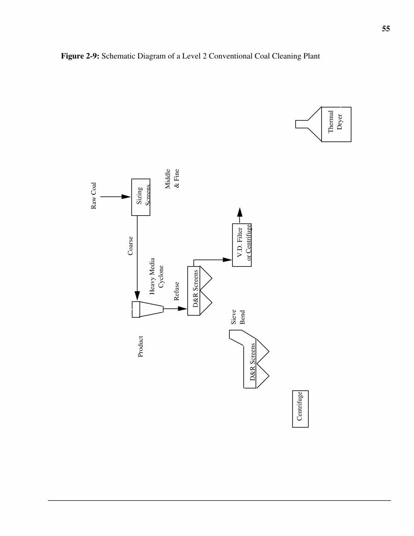
55
Figure 2-9: Schematic Diagram of a Level 2 Conventional Coal Cleaning Plant
Raw
Coa
l
Coa
rse
Mid
dle
&
Fin
e
Sizi
ng
Scre
ens
D&
R S
cree
ns
Hea
vy M
edia
C
yclo
ne
Ref
use
Prod
uct
V.D
. Filt
er
or C
entr
ifug
e
Cen
trif
uge
The
rmal
D
ryer
D&
R S
cree
ns
Siev
e B
end
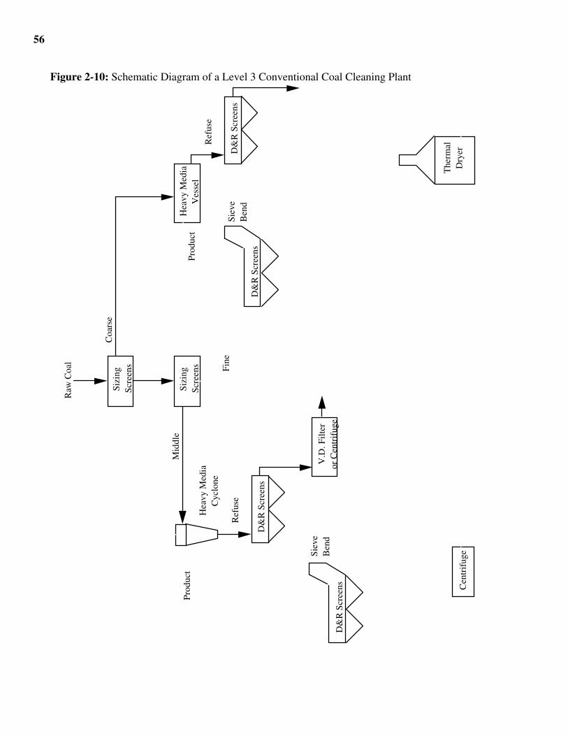
56
Figure 2-10: Schematic Diagram of a Level 3 Conventional Coal Cleaning PlantR
aw C
oal
Coa
rse
Mid
dle
Fine
D&
R S
cree
ns
Sizi
ng
Scre
ens
Sizi
ng
Scre
ens
Hea
vy M
edia
V
esse
l
D&
R S
cree
ns
Hea
vy M
edia
C
yclo
neR
efus
e
Ref
use
Pro
duct
Pro
duct
V.D
. Fil
ter
or C
entr
ifug
e
Cen
trif
uge
The
rmal
D
ryer
D&
R S
cree
ns
D&
R S
cree
ns
Siev
e B
end
Siev
e B
end
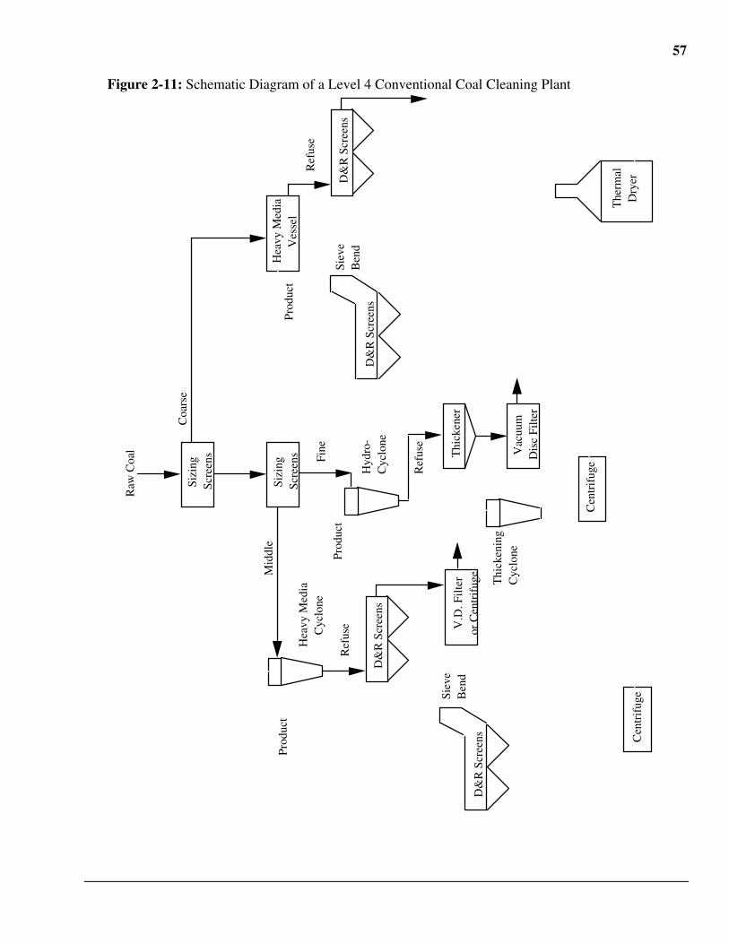
57
Figure 2-11: Schematic Diagram of a Level 4 Conventional Coal Cleaning Plant
Raw
Coa
l
Coa
rse
Mid
dle
Fine
D&
R S
cree
ns
Sizi
ng
Scre
ens
Sizi
ng
Scre
ens
Hea
vy M
edia
V
esse
l
D&
R S
cree
ns
Hea
vy M
edia
C
yclo
ne
Ref
use
Ref
use
Ref
use
Pro
duct
Pro
duct
Pro
duct
Thi
cken
er
Vac
uum
D
isc
Filte
r
V.D
. Fil
ter
or C
entr
ifug
e
Cen
trif
uge
Cen
trif
uge
The
rmal
D
ryer
D&
R S
cree
ns
D&
R S
cree
ns
Siev
e B
end
Siev
e B
end
Hyd
ro-
Cyc
lone
Thi
cken
ing
Cyc
lone
58
With the new weight fraction data it is possible to calculate the quality of the coal leaving thecoal cleaning plant. The moisture content of the final product depends on whether any streamwas thermally dried. From this, the higher heating value, ash and sulfur content on a wet basiscan be calculated with the equations shown below.
If δi = 1 then
m'o,i = m'out
else
m'o,i = m'in,i
m' o =
m' o,ifso,i
1 - m' o,ii=1
3
fso,i
1 - m' o,ii=1
3
HHVo = (1 - m' o,i) HHVo,ifso,ii=1
3
Ao = (1 - m' o,i) Ao,ifso,ii=1
3
So = (1 - m' o,i) So,ifso,ii=1
3
The quality of the final product after the thermal drier may differ slightly from the targetquality specified because the optimization algorithm is based on dry coal properties. Thedifference should not be very large since the thermal drier usually has a mass yield well above98%. Also note, that if all the streams are picked to be thermally dried, the model will onlyattempt to dry to coal if the moisture content exceeds a specified value.
59
3 COPPER OXIDE PROCESS MODEL
3.1 Nomenclature
a Slope of linear approximation of enthalpy function (Btu/lb•mole •R)A reactor cross-sectional area, m2
b Intercept of linear approximation of enthalpy function (Btu/lb•mole •R)Co initial CuO content, kg CuO/kg Al2O3Cpavg Heat capacity (Btu/•R)D fluidized bed (expanded) density, kg Al2O3/m3
E activation energy, KJ/gmoleF sorbent feed rate, kg Al2O3/hrFf frequency factor, 1/hrG molar volume of gas at reaction temperature, m3/kgmolehi Enthalpy of i (Btu/lb•mole •R)k reaction rate constant, 1/hrM molecular weight of CuO, kg/kgmolemj mass flow rate of j, lb/hrMj Molar flow rate of j, lb•mole/hrMWj molecular weight of j, lb/lb•molep fractional partial pressure of SO2 at absorber outletpo fractional partial pressure of SO2 at absorber inletQreac Total energy released or absorbed by reaction (Btu/hr)Qtotal Total energy entering device including Qreac (Btu/hr)r Molar ratio of sulfur dioxide entering absorber to available copperR universal gas constant, 0.008314 KJ/(gmole-K)Rc ratio of the molecular weights of Cu and CuOT absolute reaction temperature, KVo inlet flue gas volumetric flow rate, m3/hrxCu weight fraction of available copper in sorbent (kg Cu/kg fresh sorbent)Z expanded bed depth, m.ηr regeneration efficiency, fraction
SubcategoriesAl2O3 Alumina substrateCu CopperCuO Copper OxideCuSO4 Copper sulfates SorbentSO2 Sulfur dioxide
3.2 Introduction
This chapter describes improvements to the copper oxide process model relative to theoriginal formulation (1). The areas that were modified are the sulfation reaction algorithm in theabsorber the enthalpy functions used to calculate the temperatures of various streams and theenergy captured by the air preheater. The sulfation reaction algorithm is described below inSection 3.3. The new enthalpy functions and the heats of reactions are described in Section 2.2,while the changes in the copper oxide model caused by the new enthalpy functions are described

60
in Section 3.4. The algorithms that determined the energy captured by the air preheater aredescribed in Section 2.4. A schematic diagram of the copper oxide process is shown in Figure 3-1.
Figure 3-1: Schematic Diagram of the Copper Oxide Process
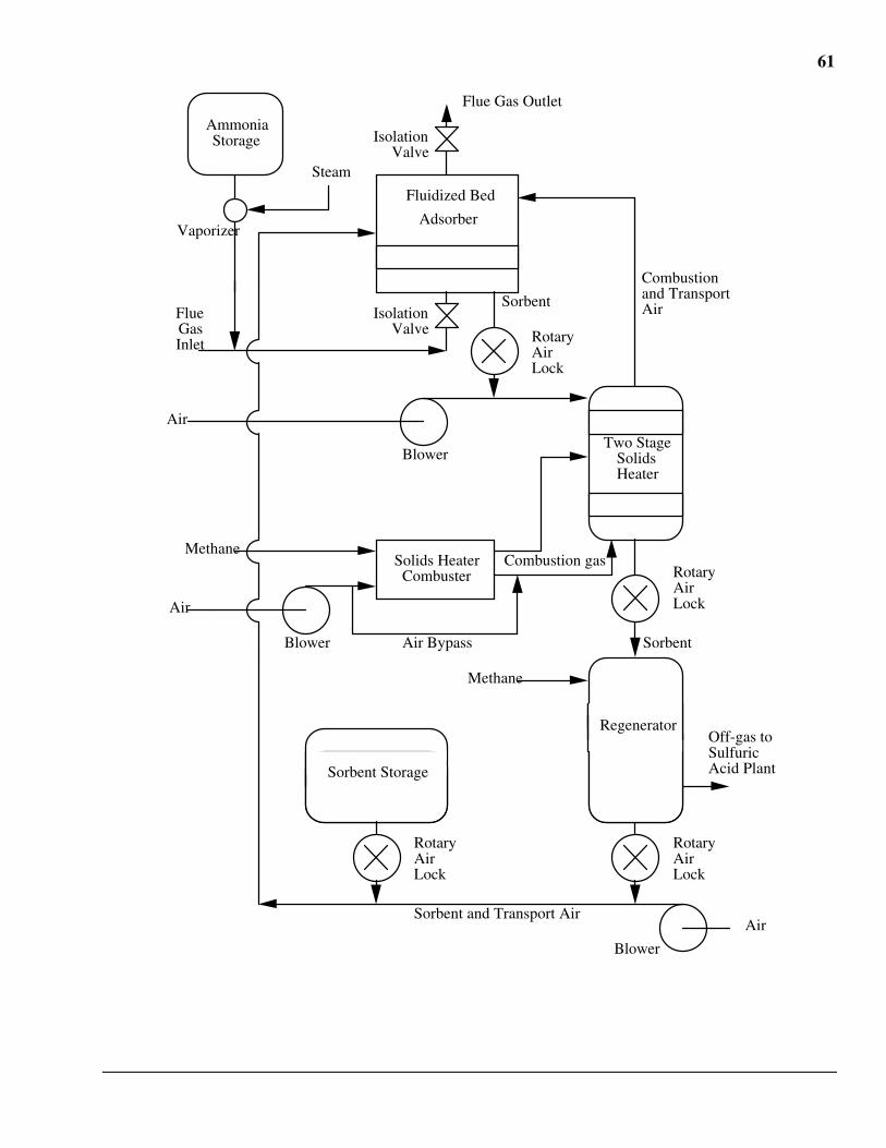
61
Fluidized Bed
Adsorber
Ammonia Storage
Steam
Flue Gas Inlet
Isolation Valve
Two Stage Solids Heater
Rotary Air Lock
Sorbent
Isolation Valve
Flue Gas Outlet
Air
Solids Heater Combuster
Air
Methane
Air Bypass
Combustion gasRotary Air Lock
Methane
Rotary Air Lock
Air
Sorbent Storage
Vaporizer
Blower
Blower
Blower
Sorbent
Sorbent and Transport Air
Combustion and Transport Air
Rotary Air Lock
RegeneratorOff-gas to Sulfuric Acid Plant
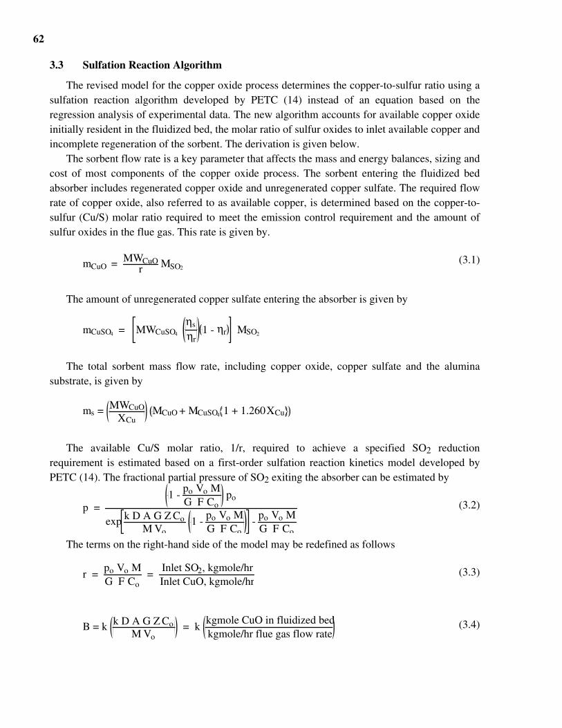
62
3.3 Sulfation Reaction Algorithm
The revised model for the copper oxide process determines the copper-to-sulfur ratio using asulfation reaction algorithm developed by PETC (14) instead of an equation based on theregression analysis of experimental data. The new algorithm accounts for available copper oxideinitially resident in the fluidized bed, the molar ratio of sulfur oxides to inlet available copper andincomplete regeneration of the sorbent. The derivation is given below.
The sorbent flow rate is a key parameter that affects the mass and energy balances, sizing andcost of most components of the copper oxide process. The sorbent entering the fluidized bedabsorber includes regenerated copper oxide and unregenerated copper sulfate. The required flowrate of copper oxide, also referred to as available copper, is determined based on the copper-to-sulfur (Cu/S) molar ratio required to meet the emission control requirement and the amount ofsulfur oxides in the flue gas. This rate is given by.
mCuO = MWCuOr MSO2
(3.1)
The amount of unregenerated copper sulfate entering the absorber is given by
mCuSO4 = MWCuSO4 ηs
ηr1 - ηr MSO2
The total sorbent mass flow rate, including copper oxide, copper sulfate and the aluminasubstrate, is given by
ms = MWCuO
XCu MCuO + MCuSO4 1 + 1.260XCu
The available Cu/S molar ratio, 1/r, required to achieve a specified SO2 reductionrequirement is estimated based on a first-order sulfation reaction kinetics model developed byPETC (14). The fractional partial pressure of SO2 exiting the absorber can be estimated by
p = 1 -
po Vo MG F Co
po
exp k D A G Z CoM Vo
1 - po Vo MG F Co
- po Vo MG F Co
(3.2)
The terms on the right-hand side of the model may be redefined as follows
r = po Vo MG F Co
= Inlet SO2, kgmole/hrInlet CuO, kgmole/hr
(3.3)
B = k k D A G Z CoM Vo
= k kgmole CuO in fluidized bedkgmole/hr flue gas flow rate
(3.4)
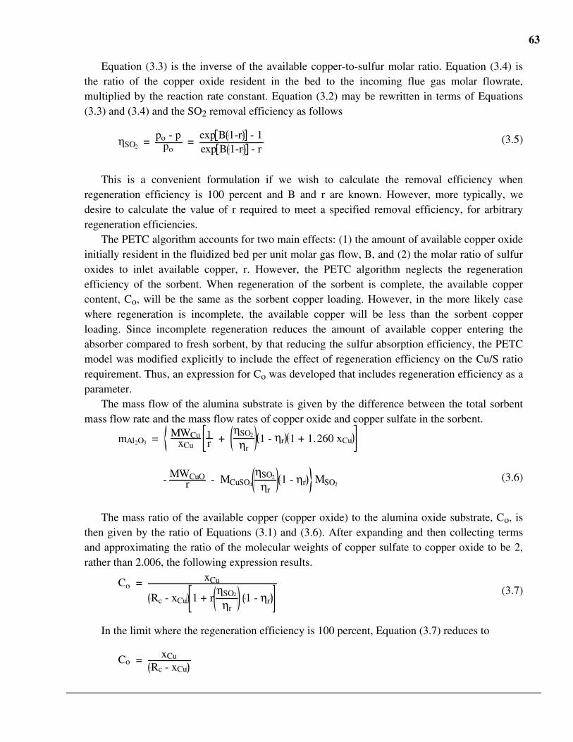
63
Equation (3.3) is the inverse of the available copper-to-sulfur molar ratio. Equation (3.4) isthe ratio of the copper oxide resident in the bed to the incoming flue gas molar flowrate,multiplied by the reaction rate constant. Equation (3.2) may be rewritten in terms of Equations(3.3) and (3.4) and the SO2 removal efficiency as follows
ηSO2 =
po - ppo
= exp B 1-r - 1exp B 1-r - r
(3.5)
This is a convenient formulation if we wish to calculate the removal efficiency whenregeneration efficiency is 100 percent and B and r are known. However, more typically, wedesire to calculate the value of r required to meet a specified removal efficiency, for arbitraryregeneration efficiencies.
The PETC algorithm accounts for two main effects: (1) the amount of available copper oxideinitially resident in the fluidized bed per unit molar gas flow, B, and (2) the molar ratio of sulfuroxides to inlet available copper, r. However, the PETC algorithm neglects the regenerationefficiency of the sorbent. When regeneration of the sorbent is complete, the available coppercontent, Co, will be the same as the sorbent copper loading. However, in the more likely casewhere regeneration is incomplete, the available copper will be less than the sorbent copperloading. Since incomplete regeneration reduces the amount of available copper entering theabsorber compared to fresh sorbent, by that reducing the sulfur absorption efficiency, the PETCmodel was modified explicitly to include the effect of regeneration efficiency on the Cu/S ratiorequirement. Thus, an expression for Co was developed that includes regeneration efficiency as aparameter.
The mass flow of the alumina substrate is given by the difference between the total sorbentmass flow rate and the mass flow rates of copper oxide and copper sulfate in the sorbent.
mAl2O3 = MWCuxCu
1r +
ηSO2
ηr1 - ηr 1 + 1.260 xCu
- MWCuOr - MCuSO4
ηSO2
ηr1 - ηr MSO2
(3.6)
The mass ratio of the available copper (copper oxide) to the alumina oxide substrate, Co, isthen given by the ratio of Equations (3.1) and (3.6). After expanding and then collecting termsand approximating the ratio of the molecular weights of copper sulfate to copper oxide to be 2,rather than 2.006, the following expression results.
Co = xCu
Rc - xCu 1 + rηSO2
ηr 1 - ηr
(3.7)
In the limit where the regeneration efficiency is 100 percent, Equation (3.7) reduces to
Co = xCu
Rc - xCu
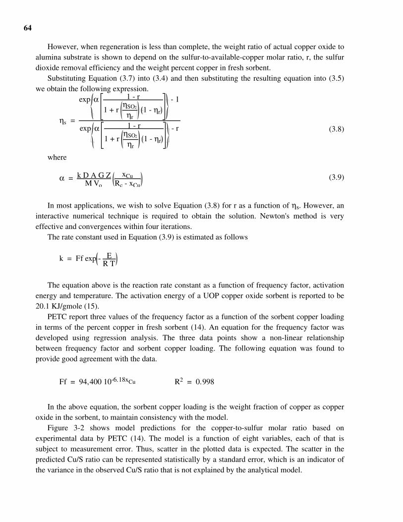
64
However, when regeneration is less than complete, the weight ratio of actual copper oxide toalumina substrate is shown to depend on the sulfur-to-available-copper molar ratio, r, the sulfurdioxide removal efficiency and the weight percent copper in fresh sorbent.
Substituting Equation (3.7) into (3.4) and then substituting the resulting equation into (3.5)we obtain the following expression.
ηs =
exp α 1 - r
1 + r ηSO2
ηr 1 - ηr
- 1
exp α 1 - r
1 + r ηSO2
ηr 1 - ηr
- r (3.8)
where
α = k D A G ZM Vo
xCuRc - xCu
(3.9)
In most applications, we wish to solve Equation (3.8) for r as a function of ηs. However, aninteractive numerical technique is required to obtain the solution. Newton's method is veryeffective and convergences within four iterations.
The rate constant used in Equation (3.9) is estimated as follows
k = Ff exp - ER T
The equation above is the reaction rate constant as a function of frequency factor, activationenergy and temperature. The activation energy of a UOP copper oxide sorbent is reported to be20.1 KJ/gmole (15).
PETC report three values of the frequency factor as a function of the sorbent copper loadingin terms of the percent copper in fresh sorbent (14). An equation for the frequency factor wasdeveloped using regression analysis. The three data points show a non-linear relationshipbetween frequency factor and sorbent copper loading. The following equation was found toprovide good agreement with the data.
Ff = 94,400 10-6.18xCu R2 = 0.998
In the above equation, the sorbent copper loading is the weight fraction of copper as copperoxide in the sorbent, to maintain consistency with the model.
Figure 3-2 shows model predictions for the copper-to-sulfur molar ratio based onexperimental data by PETC (14). The model is a function of eight variables, each of that issubject to measurement error. Thus, scatter in the plotted data is expected. The scatter in thepredicted Cu/S ratio can be represented statistically by a standard error, which is an indicator ofthe variance in the observed Cu/S ratio that is not explained by the analytical model.
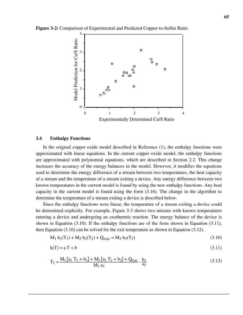
65
Figure 3-2: Comparison of Experimental and Predicted Copper-to-Sulfur Ratio
43210
0
1
2
3
4
Experimentally Determined Cu/S Ratio
Mod
el P
redi
ctio
n fo
r C
u/S
Rat
io
3.4 Enthalpy Functions
In the original copper oxide model described in Reference (1), the enthalpy functions wereapproximated with linear equations. In the current copper oxide model, the enthalpy functionsare approximated with polynomial equations, which are described in Section 2.2. This changeincreases the accuracy of the energy balances in the model. However, it modifies the equationsused to determine the energy difference of a stream between two temperatures, the heat capacityof a stream and the temperature of a stream exiting a device. Any energy difference between twoknown temperatures in the current model is found by using the new enthalpy functions. Any heatcapacity in the current model is found using the form (3.16). The change in the algorithm todetermine the temperature of a stream exiting a device is described below.
Since the enthalpy functions were linear, the temperature of a stream exiting a device couldbe determined explicitly. For example, Figure 3-3 shows two streams with known temperaturesentering a device and undergoing an exothermic reaction. The energy balance of the device isshown in Equation (3.10). If the enthalpy functions are of the form shown in Equation (3.11),then Equation (3.10) can be solved for the exit temperature as shown in Equation (3.12).
M1 h1(T1) + M2 h2(T2) + Qreac = M3 h3(T3) (3.10)
h(T) = a T + b (3.11)
T3 = M1 a1 T1 + b1 + M2 a2 T2 + b2 + Qreac
M3 a3 - b3
a3(3.12)
66
In the current copper oxide model, the enthalpy functions are of the form shown in Equation(3.13)12. Because of the form of the enthalpy functions, Equation (3.10) cannot be solved for theexit temperature explicitly. Instead a two step iteration replaces the equations in the originalcopper oxide model which determined temperatures from an energy balance. In the first step, aninitial estimate of the temperature is made using Equation (3.14)13. For the second step, the exittemperature is determined with Equation (3.15). In Equation (3.15), the inlet stream that has thegreatest effect on the exit temperature is used for T1. This two step iteration is very accurate for avariety of cases studies.
h(TR) = ATR + Be-3TR
2
3.6 - 3.24Ce5
TR +
De-6TR3
9.72 - 1.8H298.15
(3.13)
Tguess = M1 h1(T1) T1 + M2 h2(T2) T2
M1 h1(T1) + M2 h2(T2) 1 +
Qreac
Qtotal(3.14)
T3 = Qtotal - M3 h3(T1)
Cp3,avg + T1 (3.15)
where
Qtotal = M1 h1(T1) + M2 h2(T2) + Qreac
Cp3,avg = M3 h3(Tguess) - h3(T1)
Tguess - T1(3.16)
Figure 3-3: Typical Device in Copper Oxide Process
Qreac
DeviceM1 M3
M2
T 1 T 3
T 2
12 The constants A, B, C, D, and H298.15 are given in Table 2.3.13 In the current copper oxide model, the temperature of the flue gas exiting the absorber is determined with
Equation (3.14), since the correction determined by Equation (3.15) is insignificant.
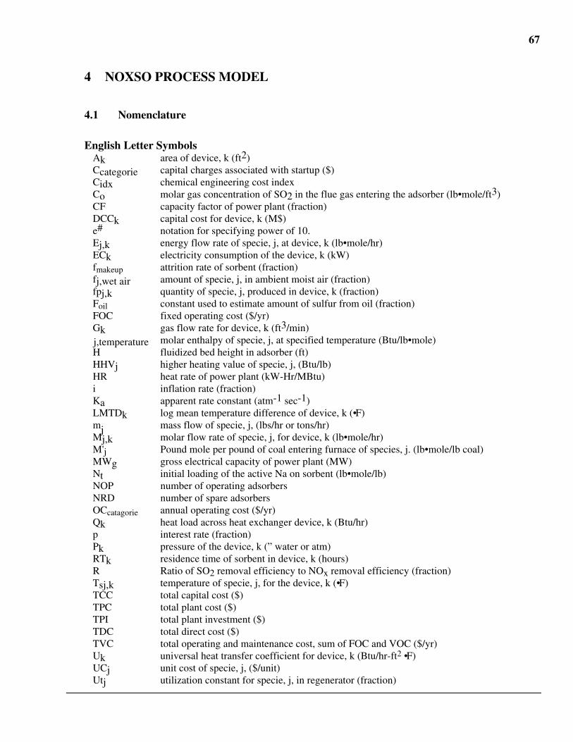
67
4 NOXSO PROCESS MODEL
4.1 Nomenclature
English Letter SymbolsAk area of device, k (ft2)Ccategorie capital charges associated with startup ($)Cidx chemical engineering cost indexCo molar gas concentration of SO2 in the flue gas entering the adsorber (lb•mole/ft3)CF capacity factor of power plant (fraction)DCCk capital cost for device, k (M$)e# notation for specifying power of 10.Ej,k energy flow rate of specie, j, at device, k (lb•mole/hr)ECk electricity consumption of the device, k (kW)fmakeup attrition rate of sorbent (fraction)fj,wet air amount of specie, j, in ambient moist air (fraction)fpj,k quantity of specie, j, produced in device, k (fraction)Foil constant used to estimate amount of sulfur from oil (fraction)FOC fixed operating cost ($/yr)Gk gas flow rate for device, k (ft3/min) ∧hj,temperature molar enthalpy of specie, j, at specified temperature (Btu/lb•mole)H fluidized bed height in adsorber (ft)HHVj higher heating value of specie, j, (Btu/lb)HR heat rate of power plant (kW-Hr/MBtu)i inflation rate (fraction)Ka apparent rate constant (atm-1 sec-1)LMTDk log mean temperature difference of device, k (•F)mj mass flow of specie, j, (lbs/hr or tons/hr)Mj,k molar flow rate of specie, j, for device, k (lb•mole/hr)M'j Pound mole per pound of coal entering furnace of species, j. (lb•mole/lb coal)MWg gross electrical capacity of power plant (MW)Nt initial loading of the active Na on sorbent (lb•mole/lb)NOP number of operating adsorbersNRD number of spare adsorbersOCcatagorie annual operating cost ($/yr)Qk heat load across heat exchanger device, k (Btu/hr)p interest rate (fraction)Pk pressure of the device, k (” water or atm)RTk residence time of sorbent in device, k (hours)R Ratio of SO2 removal efficiency to NOx removal efficiency (fraction)Tsj,k temperature of specie, j, for the device, k (•F)TCC total capital cost ($)TPC total plant cost ($)TPI total plant investment ($)TDC total direct cost ($)TVC total operating and maintenance cost, sum of FOC and VOC ($/yr)Uk universal heat transfer coefficient for device, k (Btu/hr-ft2 •F)UCj unit cost of specie, j, ($/unit)Utj utilization constant for specie, j, in regenerator (fraction)
68
V superficial velocity of flue gas through adsorber (ft/sec)VOC variable operating cost ($/yr)WNa weight fraction of sodium to sorbent (fraction)X mean value of the fractional conversion of the sorbent in the entire adsorber (fraction)y molar fraction of SO2 in the flue gas (fraction)
Greek Letter SymbolsδNOx fraction of NOx returned to boiler that is destroyed (fraction)•Hk heat of reaction in device, k (Btu/hr)ηj,k efficiency of device, k (fraction)λ molar stoichiometry of SO2 to active sorbentρsorb bulk density of sorbent (lbs/ft3)
Subscripts1 specifies the first part or half a device, kguess used to indicate the guess of a value in the interpolating algorithmsi stands for inletj,k used in sums to specify equipment or species.o stands for outletstd emission standard for either SOx or NOx
Species:acid sulfuric acidair airash ashc combustion air for gas burner not including air needed to maintain maximum
temperatureCD carbon dioxideCM carbon monoxideCS carbon oxide sulfide, COSex excess air for the gas burner needed to maintain temperatureH hydrogen, H2HS hydrogen sulfide, H2SM methane, CH4makeup makeup sorbentN nitrogen, N2NO nitrogen oxide, NOND nitrogen dioxide, NO2O oxygen, O2st steamsorb sorbentS sulfur, S2SC sulfur compounds, includes COS, H2S, S2, SO2 and SO3SD sulfur dioxide, SO2SOX sulfur dioxide and sulfur trioxideST sulfur trioxide, SO3W water, H2O
Equipment:aph air preheaterAD adsorberAH air heater for sorbent heater
69
AP acid plantB boiler of power plantGB gas burnerR regeneratorR&S regenerator and steam treatment vesselSC sorbent coolerSH sorbent heaterSTV steam treatment vessel
Categories for capital and operating cost:acid acid plantadmin support and administration laborcredit income from sale of sulfuric acideng engineering and home office feesgf general facilitiesinv inventory capitalmaint-labor maintenance labormaint-matl maintenance materialmakeup makeup catalyst due to attrition lossmarketing marketing and shipping charges for selling sulfuric acidmisc royalty and land chargesoper operating laborproc process contingencyproj project contingencystartup startup charges for one monthwork working capital
4.2 Introduction
This chapter describes improvements to the NOXSO process model originally developed byBarrett (1). Most of these changes have been reported in previous reports to PETC. (16, 17).Other minor improvements change how sulfur from the air heater is handled and modifyEquations (4.1), (4.2), (4.3), (4.7) and (4.8). Another improvement couples the SO2 and NOx
removal efficiencies in the absorber by an input parameter, R. This change modifies Equations(4.4) and (4.5).
The basic NOXSO model is based on designs by NOXSO Corporation (18-21) and Stearns-Rogers (22). The design of the process has changed over time to incorporate other potentialimprovements. The current process design for this model is based on a study for EPRI (22), withone modification suggested by NOXSO Corp (23), i.e., using methane as the reducing gasinstead of synthesis gas produced from a Texaco Coal Gasification System.
The NOXSO process is intended to remove over 90 percent of the SOx and NOx from theflue gas of a coal-fired power plant. The pollutants are adsorbed onto a sodium coated aluminasorbent in a fluidized bed reactor. The sorbent is regenerated producing various sulfurcompounds and NOx. The NOx and some SOx are returned to the boiler, while the remainingsulfur compounds are sent either to a sulfuric acid or Claus plant. The NOx returned to the boileris expected to decompose partially into nitrogen leading to a steady-state NOx concentration.
A proposed process diagram is shown in Figure 4-1. There are four major mass flows in theNOXSO process: (1) the sorbent recirculation stream, (2) the regenerator off-gas sent to the acid
70
plant, (3) the sorbent heater gas stream containing NOx and SOx returned to the boiler and (4) thecombustion/flue gas stream. This process diagram differs from the one used for the initial modeldeveloped by Barrett (1) in the following ways:
• oil is used instead of coal in the sorbent heater• the cyclone in front of the adsorber has been removed• methane is used for the reducing gas• the adsorber by-pass option has been removedFigure 4-1 is best understood by examining each major mass flow separately. The first mass
flow is the sorbent stream. The sorbent entering the adsorber contains some residual sulfurcompounds. The sorbent removes NOx and SOx from the flue gas while raising the temperatureof the flue gas. When inside the sorbent heater, it releases all the NOx and about 8 to 10 percentof the SOx in the sorbent. The sorbent then enters the regenerator where methane (or anotherreducing gas) is used to remove additional SOx in the sorbent. After the regenerator, the sorbententers the steam treatment vessel where steam is used to removed most of the remaining sulfurcompounds. Finally, the sorbent is cooled and makeup sorbent is added before it is returned tothe adsorber.
The second major mass stream is the off gas from the regenerator. This gas stream is criticalto the cost and performance of the acid plant, since its composition can drastically affect the costof the sulfur recovery system. Its composition depends on the type and quantity of reducing gasused and the design of the regenerator and steam treatment vessels. In communications withNOXSO Corporation they have suggested that these two vessels be replaced with a single vessel.
The third major stream is the air stream used to heat and cool the sorbent and to return theNOx (and some SOx) to the boiler. Recent tests have indicated that approximately 65% of theNOx returned to the boiler is decomposed (24). This air stream also contains a significant amountof oxygen, so it is used to reduce the amount of combustion air entering the air preheater. Thisgas stream enters the sorbent cooler where it is heated by cooling the sorbent to approximately210 •F. Then it enters the sorbent heater where it picks up the NOx and some SOx. After leavingthe sorbent heater it mixes with combustion air and enters the boiler.
The last mass flow is the combustion/flue gas stream. The inlet air passes through the airpreheater and picks up the gas stream exiting the sorbent heater. This gas stream contains NOx,
SOx and the products of combustion from the air heater, plus air used to heat and cool thesorbent. The inlet gas entering the air preheater is reduced in proportion to the amount of oxygenentering this stream. The SOx comes from the sorbent heater and the combustion of #6 fuel oil.This combined gas stream enters the boiler where some NOx decomposes. After the boiler itpasses through the air preheater, where it picks up additional air leaking across air preheater.After the air preheater, the flue gas is cooled by adding water. It then enters the adsorber, wheremost of the NOx and SOx are removed by the sorbent. The cleaned flue gas picks up the attritionparticles of the sorbent and enters the fabric filter. Here, particulate matter is removed before thegas is vented to the atmosphere.
Figure 4-1: NOXSO Process Diagram
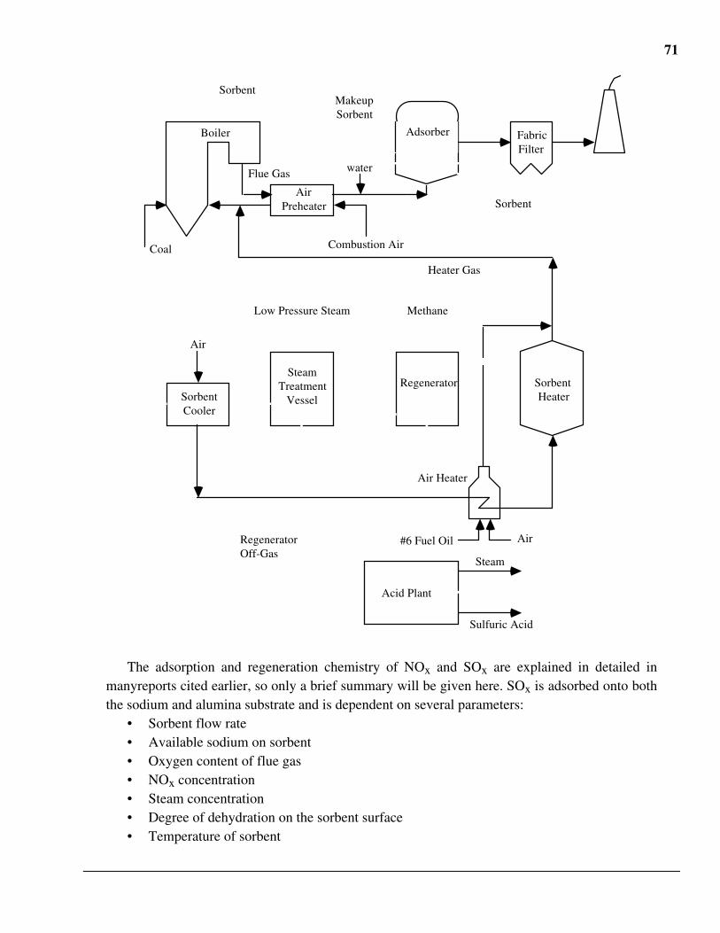
71
water
Combustion AirCoal
#6 Fuel Oil Air
Air
Sulfuric Acid
Steam
MethaneLow Pressure Steam
Acid Plant
Air Heater
Sorbent Heater
RegeneratorSteam
Treatment VesselSorbent
Cooler
Air Preheater
Adsorber Fabric Filter
Sorbent
Flue Gas
Regenerator Off-Gas
Boiler
Makeup Sorbent
Sorbent
Heater Gas
The adsorption and regeneration chemistry of NOx and SOx are explained in detailed inmanyreports cited earlier, so only a brief summary will be given here. SOx is adsorbed onto boththe sodium and alumina substrate and is dependent on several parameters:
• Sorbent flow rate• Available sodium on sorbent• Oxygen content of flue gas• NOx concentration• Steam concentration• Degree of dehydration on the sorbent surface• Temperature of sorbent
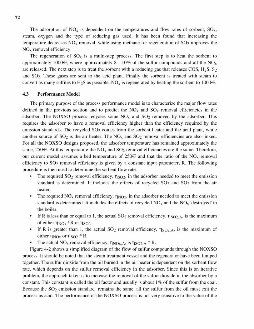
72
The adsorption of NOx is dependent on the temperatures and flow rates of sorbent, SOx,steam, oxygen and the type of reducing gas used. It has been found that increasing thetemperature decreases NOx removal, while using methane for regeneration of SO2 improves theNOx removal efficiency.
The regeneration of SOx is a multi-step process. The first step is to heat the sorbent toapproximately 1000•F, where approximately 8 - 10% of the sulfur compounds and all the NOx
are released. The next step is to treat the sorbent with a reducing gas that releases COS, H2S, S2
and SO2. These gases are sent to the acid plant. Finally the sorbent is treated with steam toconvert as many sulfites to H2S as possible. NOx is regenerated by heating the sorbent to 1000•F.
4.3 Performance Model
The primary purpose of the process performance model is to characterize the major flow ratesdefined in the previous section and to predict the NOx and SOx removal efficiencies in theadsorber. The NOXSO process recycles some NOx and SO2 removed by the adsorber. Thisrequires the adsorber to have a removal efficiency higher than the efficiency required by theemission standards. The recycled SO2 comes from the sorbent heater and the acid plant, whileanother source of SO2 is the air heater. The NOx and SO2 removal efficiencies are also linked.For all the NOXSO designs proposed, the adsorber temperature has remained approximately thesame, 250•F. At this temperature the NOx and SO2 removal efficiencies are the same. Therefore,our current model assumes a bed temperature of 250•F and that the ratio of the NOx removalefficiency to SO2 removal efficiency is given by a constant input parameter, R. The followingprocedure is then used to determine the sorbent flow rate:
• The required SO2 removal efficiency, ηSO2, in the adsorber needed to meet the emissionstandard is determined. It includes the effects of recycled SO2 and SO2 from the airheater.
• The required NOx removal efficiency, ηNOx, in the adsorber needed to meet the emissionstandard is determined. It includes the effects of recycled NOx and the NOx 'destroyed' inthe boiler.
• If R is less than or equal to 1, the actual SO2 removal efficiency, ηSO2,A, is the maximumof either ηNOx / R or ηSO2.
• If R is greater than 1, the actual SO2 removal efficiency, ηSO2,A, is the maximum ofeither ηNOx or ηSO2 * R.
• The actual NOx removal efficiency, ηNOx,A, is ηSO2,A * R.Figure 4-2 shows a simplified diagram of the flow of sulfur compounds through the NOXSO
process. It should be noted that the steam treatment vessel and the regenerator have been lumpedtogether. The sulfur dioxide from the oil burned in the air heater is dependent on the sorbent flowrate, which depends on the sulfur removal efficiency in the adsorber. Since this is an iterativeproblem, the approach taken is to increase the removal of the sulfur dioxide in the absorber by aconstant. This constant is called the oil factor and usually is about 1% of the sulfur from the coal.Because the SO2 emission standard remains the same, all the sulfur from the oil must exit theprocess as acid. The performance of the NOXSO process is not very sensitive to the value of the
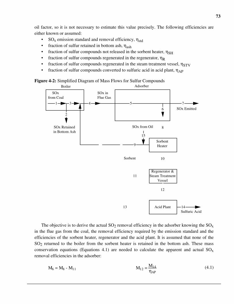
73
oil factor, so it is not necessary to estimate this value precisely. The following efficiencies areeither known or assumed:
• SOx emission standard and removal efficiency, ηstd• fraction of sulfur retained in bottom ash, ηash• fraction of sulfur compounds not released in the sorbent heater, ηSH• fraction of sulfur compounds regenerated in the regenerator, ηR• fraction of sulfur compounds regenerated in the steam treatment vessel, ηSTV• fraction of sulfur compounds converted to sulfuric acid in acid plant, ηAP
Figure 4-2: Simplified Diagram of Mass Flows for Sulfur CompoundsAdsorber
SOx in Flue Gas
SOx Emitted
1
2
3 4 5
6
7
Sorbent Heater
Regenerator & Steam Treatment
Vessel
Sorbent
8
10
9
11
Acid PlantSulfuric Acid
12
13 14
Boiler
SOx Retained in Bottom Ash
SOx from Coal
15
SOx from Oil
The objective is to derive the actual SO2 removal efficiency in the adsorber knowing the SOx
in the flue gas from the coal, the removal efficiency required by the emission standard and theefficiencies of the sorbent heater, regenerator and the acid plant. It is assumed that none of theSO2 returned to the boiler from the sorbent heater is retained in the bottom ash. These massconservation equations (Equations 4.1) are needed to calculate the apparent and actual SOx
removal efficiencies in the adsorber:
M6 = M8 - M11 M12 = M14ηAP
(4.1)
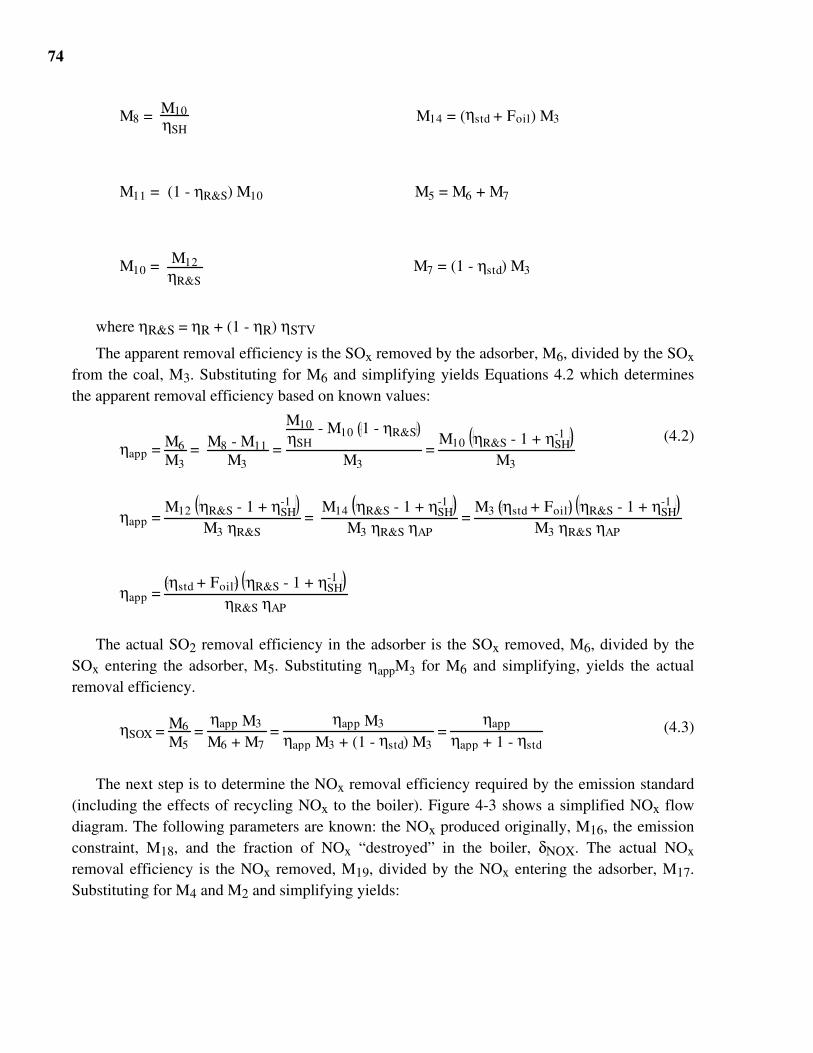
74
M8 = M10ηSH
M14 = (ηstd + Foil) M3
M11 = (1 - ηR&S) M10 M5 = M6 + M7
M10 = M12ηR&S
M7 = (1 - ηstd) M3
where ηR&S = ηR + (1 - ηR) ηSTV
The apparent removal efficiency is the SOx removed by the adsorber, M6, divided by the SOx
from the coal, M3. Substituting for M6 and simplifying yields Equations 4.2 which determinesthe apparent removal efficiency based on known values:
ηapp = M6M3
= M8 - M11M3
=
M10ηSH
- M10 1 - ηR&S
M3 =
M10 ηR&S - 1 + ηSH-1
M3
(4.2)
ηapp = M12 ηR&S - 1 + ηSH
-1
M3 ηR&S =
M14 ηR&S - 1 + ηSH-1
M3 ηR&S ηAP =
M3 ηstd + Foil ηR&S - 1 + ηSH-1
M3 ηR&S ηAP
ηapp = ηstd + Foil ηR&S - 1 + ηSH
-1
ηR&S ηAP
The actual SO2 removal efficiency in the adsorber is the SOx removed, M6, divided by theSOx entering the adsorber, M5. Substituting ηappM3 for M6 and simplifying, yields the actualremoval efficiency.
ηSOX = M6
M5 =
ηapp M3
M6 + M7 =
ηapp M3
ηapp M3 + (1 - ηstd) M3 =
ηapp
ηapp + 1 - ηstd(4.3)
The next step is to determine the NOx removal efficiency required by the emission standard(including the effects of recycling NOx to the boiler). Figure 4-3 shows a simplified NOx flowdiagram. The following parameters are known: the NOx produced originally, M16, the emissionconstraint, M18, and the fraction of NOx “destroyed” in the boiler, δNOX. The actual NOx
removal efficiency is the NOx removed, M19, divided by the NOx entering the adsorber, M17.Substituting for M4 and M2 and simplifying yields:
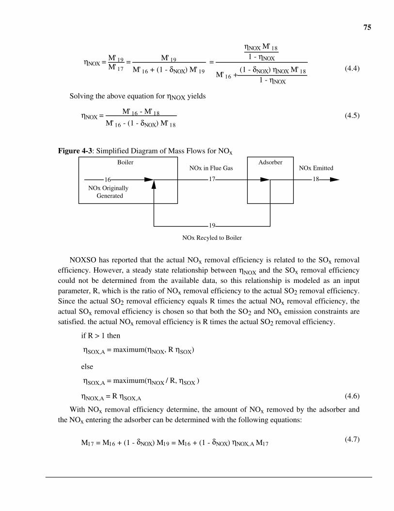
75
ηNOX = M' 19M' 17
= M' 19
M' 16 + (1 - δNOX) M' 19
=
ηNOX M' 18
1 - ηNOX
M' 16 + (1 - δNOX) ηNOX M' 18
1 - ηNOX
(4.4)
Solving the above equation for ηNOX yields
ηNOX = M' 16 - M' 18
M' 16 - (1 - δNOX) M' 18
(4.5)
Figure 4-3: Simplified Diagram of Mass Flows for NOx
Boiler Adsorber
16 17 18
19
NOx Recyled to Boiler
NOx Originally Generated
NOx EmittedNOx in Flue Gas
NOXSO has reported that the actual NOx removal efficiency is related to the SOx removalefficiency. However, a steady state relationship between ηNOX and the SOx removal efficiencycould not be determined from the available data, so this relationship is modeled as an inputparameter, R, which is the ratio of NOx removal efficiency to the actual SO2 removal efficiency.Since the actual SO2 removal efficiency equals R times the actual NOx removal efficiency, theactual SOx removal efficiency is chosen so that both the SO2 and NOx emission constraints aresatisfied. the actual NOx removal efficiency is R times the actual SO2 removal efficiency.
if R > 1 then
ηSOX,A = maximum(ηNOX, R ηSOX)
else
ηSOX,A = maximum(ηNOX / R, ηSOX )
ηNOX,A = R ηSOX,A (4.6)
With NOx removal efficiency determine, the amount of NOx removed by the adsorber andthe NOx entering the adsorber can be determined with the following equations:
M17 = M16 + (1 - δNOX) M19 = M16 + (1 - δNOX) ηNOX,A M17(4.7)
76
M17 = M16
1 - (1 - δNOX) ηNOX,A
(4.8)
M19 = ηNOX,AM17
With the actual SOx removal efficiency in the adsorber known, it is possible to determine theSOx removed by the adsorber and the SOx remaining in the flue gas. Equations 4.6, 4.7 and 4.9are easily derived from Figure 4-2. The derivation of Equation 4.8 is quite involved and is notpresented here. The ratio of sulfur exiting the absorber to the sulfur removed by the absorber is
c = M6
M8 = 1 - (1 - ηR&S) ηSH (4.9)
M7 = M5 (1 - ηSO2,A)
M6 = M3 ηSO2,A c (1 + Foil)
c - ηSO2,A (1 - ηSH + (1 - ηAP) ηR&S ηSH)
M8 = M6c
The sorbent flow rate is determined by an algorithm developed by NOXSO (24). Thenumerator in Equation 4.10 is the SOx removed by the adsorber, M6. λ is the stoichiometric ratioof sulfur removed to available sodium and is assumed to be unity (23). The parameter X can bedetermined by existing algorithms (24).
msorb
= λNtX
AAVCo(y
i - yo)
= λNtX
M6 (4.10)
X = kaPH
ln y
i
yo V
+ 1= kaPH
ln(1 - ηSOX,A
)V + 1
H, Ka, P and λ are input parameters. Ka is currently set to 3.7 according to (24), while P isassumed to be 1 atmosphere. Nt is the loading of active sorbent material to the weight of sorbent.This can be determined by the following equation:
Nt = 23 η
R&S
wNa
Once the sorbent flow rate is known, the makeup sorbent rate and the energy required topump the sorbent can be determined. The makeup sorbent rate is assumed to be a fraction of the
77
sorbent rate and is an input parameter. Energy to pump the sorbent is assumed to be proportionalto the energy estimated in the EPRI report (22):
mmakeup = fmakeup msorb
ECsorb = 1795 kW / 1.3486e6 lb/hr * msorb = 1.32e-3 msorb
The energy required to raise the sorbent temperature to 1110•F from the exit temperature ofthe adsorber is simply the difference in enthalpy times the sorbent flow rate. This determines theamount of air needed by the sorbent heater. It is assumed that the air temperature drops from1280•F to 610•F in the sorbent heater.
Esorb,SH = ( ∧hsorb(1110) -
∧hsorb(250)) msorb
Mair,SH
= ∧h
air(1,280) -
∧h
air(610)
Esorb,SH
Once the flow rate of the air is determined, the amount of energy needed to heat the air to1280•F is equal to the energy flow rate of air at 1280•F minus the heat given up in the sorbentcooler minus the energy flow rate of air at 100•F, which is the temperature of the air after thecompressor. The sorbent flow rate at the sorbent cooler is approximately 7% less than when itleft the adsorber; it is also assumed to drop from 970•F to 210•F.
The energy required to heat the air determines the oil requirement for the air heater. Theefficiency of the air heater is an input parameter. The electricity consumption of the compressoris determined by the flow rate of air and the pressure increase, which is assumed to be 84” ofwater.
Eair,AH
= (∧h
air(1280) -
∧h
air(100))
Mair,SH
- 0.93 (∧h
sorb(970) -
∧h
sorb(210))
msorb
ECair,SH
= 0.75*60*44,240
1,545Mair,SH
1.4-1
1.4
14.68714.687 + 3.612e-2*84
1.41.4-1
- 1
(80 + 460)
Once the energy requirement to heat the air is known, this determines the oil requirement forthe air heater. The efficiency of the air heater is an input parameter and 18% excess air isassumed. With the oil consumption known, the amount of combustion air for the air heater canbe determined. The oil is assumed to be a heavy fuel oil, with a higher heating value of 18,400Btu/lb and the following composition: 87.87% carbon, 10.33% hydrogen, 1.16% sulfur, 0.14%nitrogen and 0.50% oxygen (8). The actual composition is not extremely critical, yet thecomponents are in place in case another fuel, such as coal, is used.
moil
= HHV
oilη
AH
Eair,SH
78
mair,AH
= fO, wet air
120.8787 +
40.1033 +
320.0116 -
320.005
1.18m
oil
The amount of steam and methane used in the regenerator and steam treatment vessels can becalculated once the sulfur flow rate exiting the sorbent heater is found. The methane requirementfor the regenerator is assumed to be proportional to the sulfur dioxide entering the regenerator.According to NOXSO, approximately 3690 SCFM of methane are needed for 575 lb-moles perhour of sulfur dioxide (25). Also 3.34 moles of steam are needed for each mole of sulfur dioxideentering the steam treatment vessel. The constant converting SCFM to lb-moles/hr is 0.1585assuming at standard temperature of 58•F.
MSC,R,i = MSC,A,o ηSH
MM,R,i = 3690 / 575 * 0.1585MSC,R,i
MW,STV,i = 3.34 (1 - ηSTV) MSC,R,i
The utilization of methane and steam and the fractions of SO2, H2S and S2 produced in theregenerator are input parameters. It is assumed that there is sufficient oxygen to convert all thecarbon in the methane to CO2, that no COS is formed and that all only H2S and steam areproduced in the steam treatment vessels. The moisture content of the regenerator gas is assumedto be the steam not used in the steam treatment vessel plus the hydrogen released when methaneis converted to carbon dioxide minus the hydrogen used to form hydrogen sulfide. This gas issent to either a sulfuric acid plant or an elemental sulfur (Claus) plant.
MM,R,o = (1 - ηR)MM,R,i
MSD,R,o = fpSD,R ηRMSD,R,i
MHS,R,o = (fpHS,R ηR + (1 - ηR)ηSTV)MSD,R,i
MS,R,o = (1 - fpSD,R - fpHS,R)ηRMSD,R,i / 2
MM,R,o = (1 - UtM) MM,R,i
MCD,R,o = UtM MM,R,i
MW,R,o = (1 - UtW)MW,STV,i + 2MCD,R,o - fpHS,R ηR MSD,R,i
The next step is to determine the composition of the gas returned to the boiler. This gasstream consists of three other streams. The first is the air used to heat and cool the sorbent,Mair,SH. The second is the NOx and SOx picked up by this stream in the sorbent heater. Finally,there is the flue gas from the air heater. The off gas from the acid plant is returned to the flue gasupstream of the adsorber. Since it is a small stream and to simplify the calculations, it is treatedas SO2 returned to the boiler. It is assumed that only SO2 is returned to the boiler from thesorbent heater, acid plant and air heater. The composition of NOx returned to the boiler isassumed to be in the same proportions as that generated in the boiler. The temperature of this gasstream is estimated to be 620•F (22).
79
MN,B,i = fN,wet airMair,SH+ 0.0014 / 28 Moil
MO,B,i = fO,wet air(Mair,SH+ 0.18 / 1.18 Mair,AH)
MW,B,i = fW,wet air(Mair,SH+ Mair,AH) + 0.1033 / 2 Moil
MCD,B,i = 0.8787 / 12 Moil
MSD,B,i = [(1 - ηSH) + (1 - ηAP)ηSHηR&S)]MSD,A,o + 0.0116 / 32 Moil
MNO,B,i = fpNO,BMNOX,A,o
MND,B,i = (1 - fpNO,B)MNOX,A,o
Now the inlet combustion air and the composition of the flue gas exiting the boiler can bedetermined. The oxygen being returned to the boiler reduces the combustion air entering the airpreheater. Since the nitrogen and moisture are based on the oxygen content, the only variablewhich needs to be modified is the oxygen required. See Chapter 2 for more details on how thevariables, MB,i, are determined. Once these parameters are known, the composition of the fluegas exiting the boiler can be determined:
MO,AP,i = MO,required - MO,B,i
MCD,B,o = MC,coal + MCD,B,i
MW,B,o = MW,coal + MW,AP,i + 0.5 MH,coal + MW,B,i
MSD,B,o = fpSD,B ηash MS,coal + MSD,B,i
MST,B,o = (1 - fpSD,B) ηash MS,coal
MND,orig
=
46 + 1 - fp
NO,B
30fpNO,B
NOxefm
coal
MNO,orig
= 1 - fp
NO,B
fpNO,B
MND,orig
MND,B,o = MND,orig + (1 - δNOX)MND,B,i
MNO,B,o = MNO,orig + (1 - δNOX)MNO,B,i
MN,B,o = 0.5MN,coal + MN,AP,i - 0.5(MNO,orig + MND,orig) + MN,B,i + 0.5MNOX,A,o
MO,B,o = MO,AP,i + 0.5MO,coal - MC,coal - 0.25MH,coal - fpSD,BηashMS,coal - 1.5MST,B,o
- 0.5MNO,orig - MND,orig + MO,B,i + δNOX(MND,B,i + 0.5MNO,B,i)
With the flue gas flow rate and combustion air determined, the air preheater model can beused to determine the flue gas temperature leaving the air preheater, Tfg,AP,o and the temperatureof the combustion exiting the air preheater, Tair,AP,o. Now the amount of water added to cool the
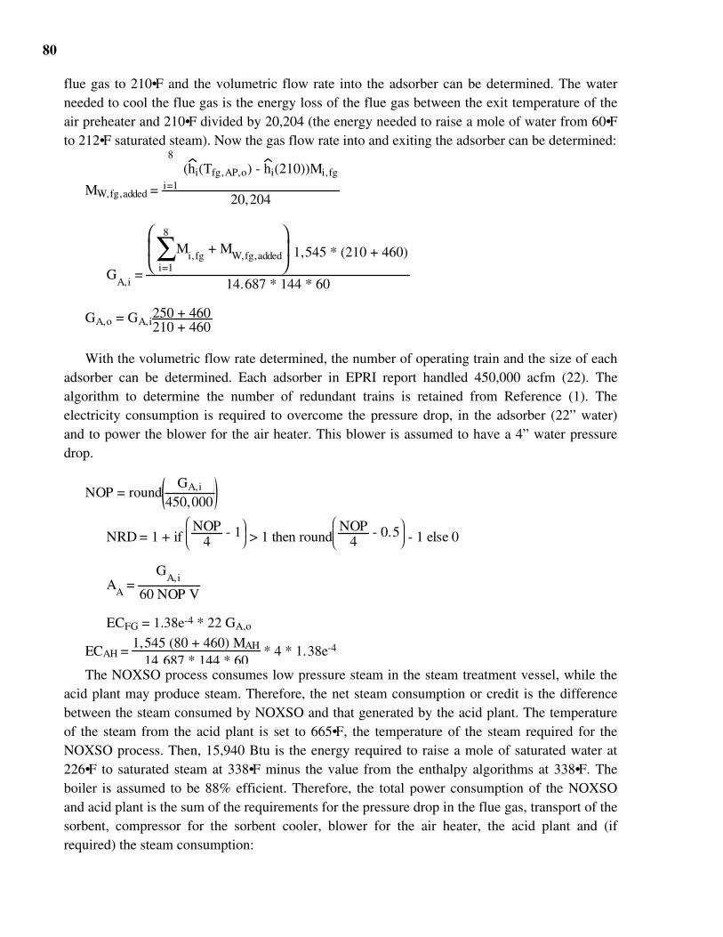
80
flue gas to 210•F and the volumetric flow rate into the adsorber can be determined. The waterneeded to cool the flue gas is the energy loss of the flue gas between the exit temperature of theair preheater and 210•F divided by 20,204 (the energy needed to raise a mole of water from 60•Fto 212•F saturated steam). Now the gas flow rate into and exiting the adsorber can be determined:
MW,fg,added =
(hi(Tfg,AP,o) - hi(210))Mi,fgi=1
8
20,204
GA,i
= 14.687 * 144 * 60
∑i=1
8
Mi,fg
+ MW,fg,added
1,545 * (210 + 460)
GA,o = GA,i250 + 460210 + 460
With the volumetric flow rate determined, the number of operating train and the size of eachadsorber can be determined. Each adsorber in EPRI report handled 450,000 acfm (22). Thealgorithm to determine the number of redundant trains is retained from Reference (1). Theelectricity consumption is required to overcome the pressure drop, in the adsorber (22” water)and to power the blower for the air heater. This blower is assumed to have a 4” water pressuredrop.
NOP = roundGA,i
450,000
NRD = 1 + if 4NOP - 1
> 1 then round
4NOP - 0.5
- 1 else 0
AA =
60 NOP V
GA,i
ECFG = 1.38e-4 * 22 GA,o
ECAH = 1,545 (80 + 460) MAH
14.687 * 144 * 60 * 4 * 1.38e-4
The NOXSO process consumes low pressure steam in the steam treatment vessel, while theacid plant may produce steam. Therefore, the net steam consumption or credit is the differencebetween the steam consumed by NOXSO and that generated by the acid plant. The temperatureof the steam from the acid plant is set to 665•F, the temperature of the steam required for theNOXSO process. Then, 15,940 Btu is the energy required to raise a mole of saturated water at226•F to saturated steam at 338•F minus the value from the enthalpy algorithms at 338•F. Theboiler is assumed to be 88% efficient. Therefore, the total power consumption of the NOXSOand acid plant is the sum of the requirements for the pressure drop in the flue gas, transport of thesorbent, compressor for the sorbent cooler, blower for the air heater, the acid plant and (ifrequired) the steam consumption:
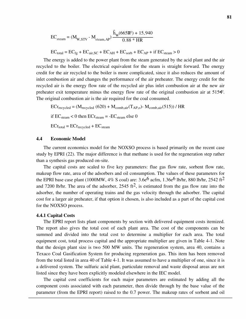
81
ECsteam = (MW,STV
- Msteam,AP
) 0.88 * HR
∧h
W(665ÞF) + 15,940
ECtotal = ECfg + ECair,SC + ECAH + ECsorb + ECAP + if ECsteam > 0
The energy is added to the power plant from the steam generated by the acid plant and the airrecycled to the boiler. The electrical equivalent for the steam is straight forward. The energycredit for the air recycled to the boiler is more complicated, since it also reduces the amount ofinlet combustion air and changes the performance of the air preheater. The energy credit for therecycled air is the energy flow rate of the recycled air plus inlet combustion air at the new airpreheater exit temperature minus the energy flow rate of the original combustion air at 515•F.The original combustion air is the air required for the coal consumed.
ECrrecycled = (Mrecycled ∧h(620) + Mcomb,air
∧h
(TAP,o)- Mcomb,air ∧h
(515)) / HR
if ECsteam < 0 then ECrsteam = -ECsteam else 0
ECrtotal = ECrrecycled + ECsteam
4.4 Economic Model
The current economics model for the NOXSO process is based primarily on the recent casestudy by EPRI (22). The major difference is that methane is used for the regeneration step ratherthan a synthesis gas produced on-site.
The capital costs are scaled to five key parameters: flue gas flow rate, sorbent flow rate,makeup flow rate, area of the adsorbers and oil consumption. The values of these parameters forthe EPRI base case plant (1000MW, 4% S coal) are: 3.6e6 acfm, 1.36e6 lb/hr, 880 lb/hr, 2542 ft2
and 7200 lb/hr. The area of the adsorber, 2545 ft2, is estimated from the gas flow rate into theadsorber, the number of operating trains and the gas velocity through the adsorber. The capitalcost for a larger air preheater, if that option it chosen, is also included as a part of the capital costfor the NOXSO process.
4.4.1 Capital CostsThe EPRI report lists plant components by section with delivered equipment costs itemized.
The report also gives the total cost of each plant area. The cost of the components can besummed and divided into the total cost to determine a multiplier for each area. The totalequipment cost, total process capital and the appropriate multiplier are given in Table 4-1. Notethat the design plant size is two 500 MW units. The regeneration system, area 40, contains aTexaco Coal Gasification System for producing regeneration gas. This item has been removedfrom the total listed in area 40 of Table 4-1. It was assumed to have a multiplier of one, since it isa delivered system. The sulfuric acid plant, particulate removal and waste disposal areas are notlisted since they have been explicitly modeled elsewhere in the IEC model.
The capital cost coefficients for each major parameters are estimated by adding all thecomponent costs associated with each parameter, then divide through by the base value of theparameter (from the EPRI report) raised to the 0.7 power. The makeup rates of sorbent and oil
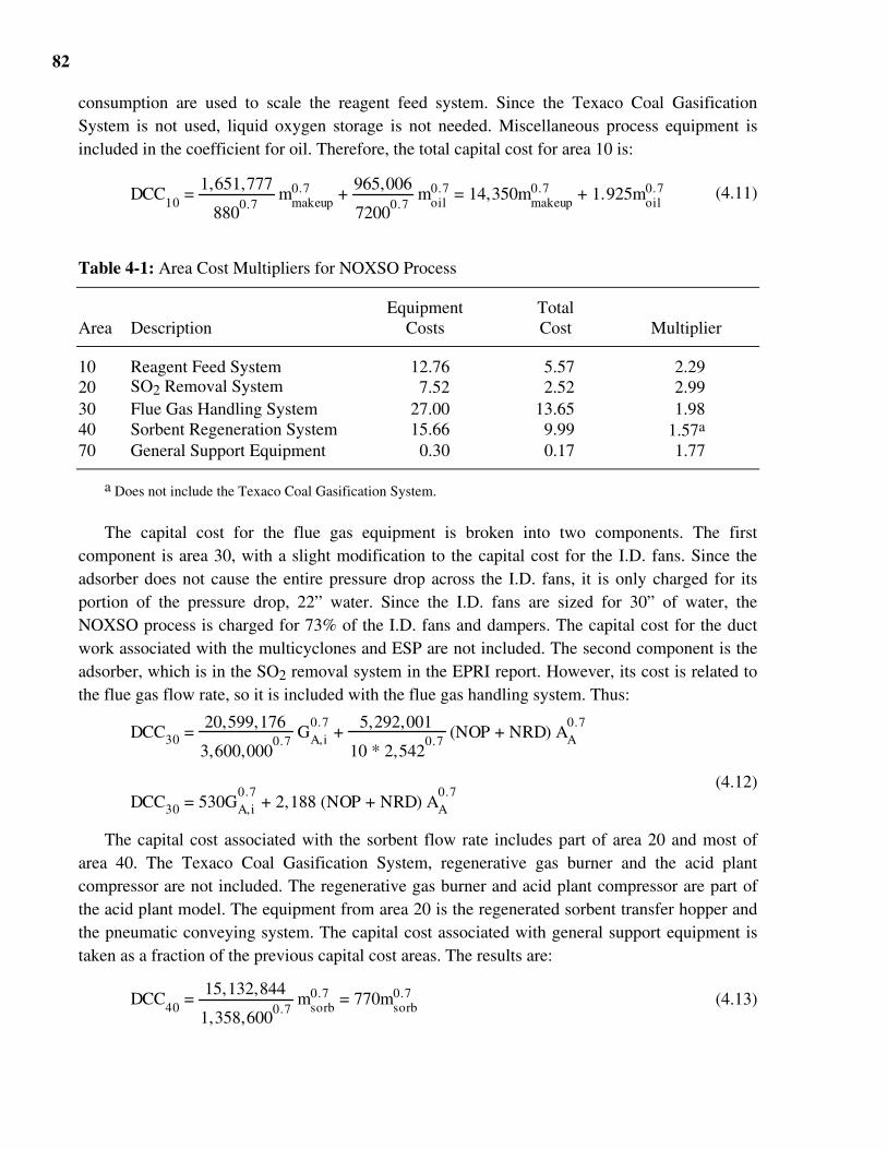
82
consumption are used to scale the reagent feed system. Since the Texaco Coal GasificationSystem is not used, liquid oxygen storage is not needed. Miscellaneous process equipment isincluded in the coefficient for oil. Therefore, the total capital cost for area 10 is:
DCC10
= 880
0.7
1,651,777 m
makeup0.7 +
72000.7
965,006 m
oil0.7 = 14,350m
makeup0.7 + 1.925m
oil0.7 (4.11)
Table 4-1: Area Cost Multipliers for NOXSO Process
Equipment TotalArea Description Costs Cost Multiplier
10 Reagent Feed System 12.76 5.57 2.2920 SO2 Removal System 7.52 2.52 2.9930 Flue Gas Handling System 27.00 13.65 1.9840 Sorbent Regeneration System 15.66 9.99 1.57a
70 General Support Equipment 0.30 0.17 1.77
a Does not include the Texaco Coal Gasification System.
The capital cost for the flue gas equipment is broken into two components. The firstcomponent is area 30, with a slight modification to the capital cost for the I.D. fans. Since theadsorber does not cause the entire pressure drop across the I.D. fans, it is only charged for itsportion of the pressure drop, 22” water. Since the I.D. fans are sized for 30” of water, theNOXSO process is charged for 73% of the I.D. fans and dampers. The capital cost for the ductwork associated with the multicyclones and ESP are not included. The second component is theadsorber, which is in the SO2 removal system in the EPRI report. However, its cost is related tothe flue gas flow rate, so it is included with the flue gas handling system. Thus:
DCC30 = 3,600,000
0.720,599,176
GA,i0.7
+ 10 * 2,542
0.75,292,001
(NOP + NRD) AA0.7
DCC30 = 530GA,i0.7
+ 2,188 (NOP + NRD) AA0.7
(4.12)
The capital cost associated with the sorbent flow rate includes part of area 20 and most ofarea 40. The Texaco Coal Gasification System, regenerative gas burner and the acid plantcompressor are not included. The regenerative gas burner and acid plant compressor are part ofthe acid plant model. The equipment from area 20 is the regenerated sorbent transfer hopper andthe pneumatic conveying system. The capital cost associated with general support equipment istaken as a fraction of the previous capital cost areas. The results are:
DCC40
= 1,358,600
0.7
15,132,844 m
sorb0.7 = 770m
sorb0.7 (4.13)
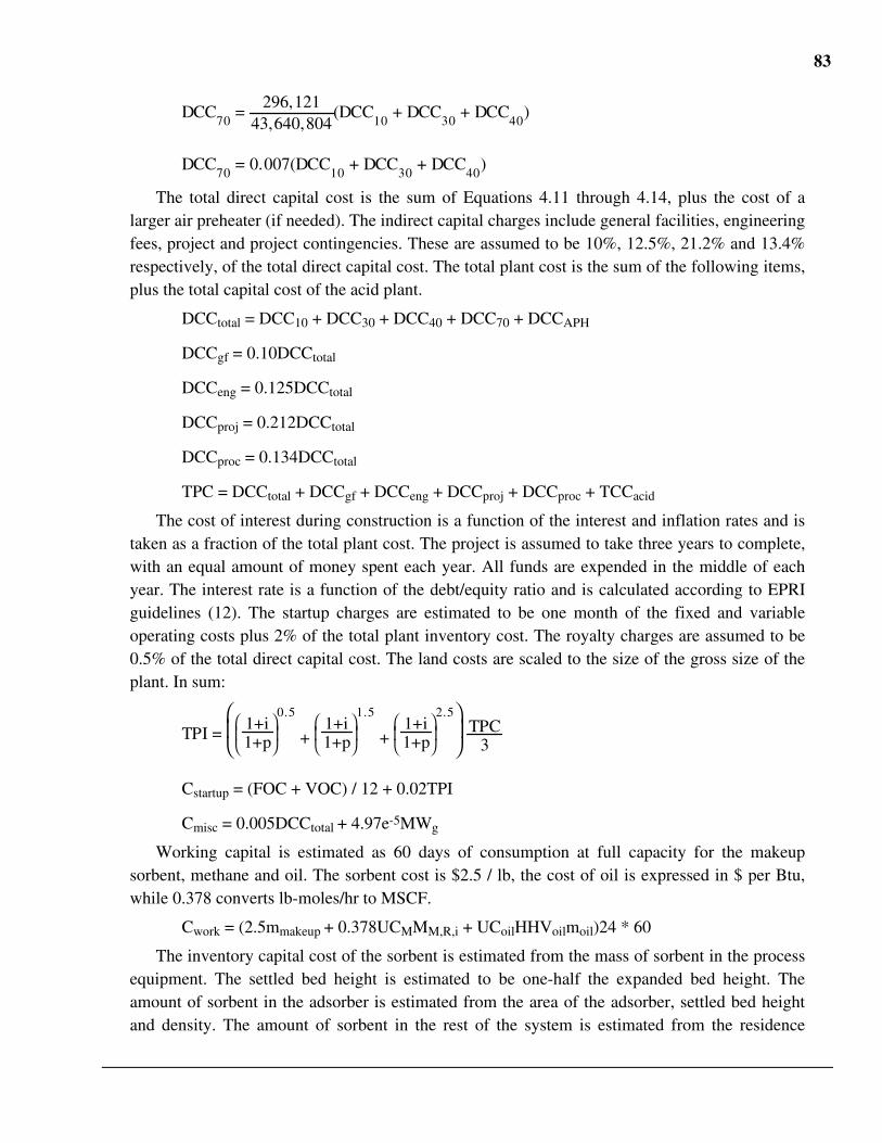
83
DCC70
= 43,640,804
296,121(DCC
10 + DCC
30 + DCC
40)
DCC70
= 0.007(DCC10
+ DCC30
+ DCC40
)
The total direct capital cost is the sum of Equations 4.11 through 4.14, plus the cost of alarger air preheater (if needed). The indirect capital charges include general facilities, engineeringfees, project and project contingencies. These are assumed to be 10%, 12.5%, 21.2% and 13.4%respectively, of the total direct capital cost. The total plant cost is the sum of the following items,plus the total capital cost of the acid plant.
DCCtotal = DCC10 + DCC30 + DCC40 + DCC70 + DCCAPH
DCCgf = 0.10DCCtotal
DCCeng = 0.125DCCtotal
DCCproj = 0.212DCCtotal
DCCproc = 0.134DCCtotal
TPC = DCCtotal + DCCgf + DCCeng + DCCproj + DCCproc + TCCacid
The cost of interest during construction is a function of the interest and inflation rates and istaken as a fraction of the total plant cost. The project is assumed to take three years to complete,with an equal amount of money spent each year. All funds are expended in the middle of eachyear. The interest rate is a function of the debt/equity ratio and is calculated according to EPRIguidelines (12). The startup charges are estimated to be one month of the fixed and variableoperating costs plus 2% of the total plant inventory cost. The royalty charges are assumed to be0.5% of the total direct capital cost. The land costs are scaled to the size of the gross size of theplant. In sum:
TPI =
1+p
1+i
0.5
+ 1+p
1+i
1.5
+ 1+p
1+i
2.5
3TPC
Cstartup = (FOC + VOC) / 12 + 0.02TPI
Cmisc = 0.005DCCtotal + 4.97e-5MWg
Working capital is estimated as 60 days of consumption at full capacity for the makeupsorbent, methane and oil. The sorbent cost is $2.5 / lb, the cost of oil is expressed in $ per Btu,while 0.378 converts lb-moles/hr to MSCF.
Cwork = (2.5mmakeup + 0.378UCMMM,R,i + UCoilHHVoilmoil)24 * 60
The inventory capital cost of the sorbent is estimated from the mass of sorbent in the processequipment. The settled bed height is estimated to be one-half the expanded bed height. Theamount of sorbent in the adsorber is estimated from the area of the adsorber, settled bed heightand density. The amount of sorbent in the rest of the system is estimated from the residence
84
times of equipment and the mass flow rate of sorbent. The total capital cost is the sum of the totalplant inventory, startup charges, working capital, inventory cost, land and royalty fees:
Cinv
= 2H A
Aρsorb +
NOP
msorb (RT
R + RT
SH + RT
SC) (NOP + NRD) * 2.5
TCC = TPI + Cstartup + Cwork + Cinv + Cmisc
4.4.2 Operating and Maintenance CostsAnnual operating charges consist of fixed and variables charges. The fixed charges consist of
the operating, maintenance, administrative labor and the maintenance materials. It is estimatedthat 5.2 workers per hour at $19.70/hr are needed for operating labor. Maintenance labor andmaterials and administration labor charges are estimated using the EPRI guidelines (12).Maintenance cost is 4.8% of the total plant cost excluding the total capital cost for the acid plant.Labor accounts for 40%, while materials account for 60% of the total maintenance cost.Administrative and support labor is estimated to be 30% of the operating and maintenance labor.The variable charges include the costs for makeup sorbent, methane, oil and miscellaneouscharges. The result is:
OCoper = 5.2 * 19.7 * 8766
OCmaint-labor = 0.40 * 0.048 (TPC - TCCacid)
OCmaint-matl = 0.60 * 0.048 (TPC - TCCacid)
OCadmin = 0.30(OCoper + OCmaint-labor)
FOC = OCoper + OCmaint-labor + OCmaint-matl + OCadmin
OCsorb = 2.5 * 8,766 CF mmakeup
OCM = 0.378 * 8,766 CF UCM MM,R,i
OCoil = 8,766 CF HHVoil UCoil moil
OCmisc = 0.019DCCtotal
VOC = OCsorb + OCM + OCoil + OCmisc
The NOXSO process typically produces an energy credit. In the IEC model, energy creditsare account for by increasing the output of the power plant while keeping coal consumption thesame. The capital and operating costs, including the additional energy cost, of the increased sizeare charged to the basic power plant, while the NOXSO process is given a credit for the energy itsupplies to the power plant. This is equivalent to if the NOXSO process decreases the amount ofcoal burned in the boiler. Since the energy credit and the cost of the NOXSO are dependent onthe coal consumption, it becomes an iterative problem.
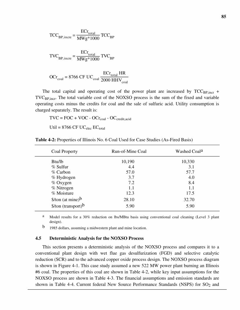
85
TCCBP,incre = MWg*1000
ECrtotal TCCBP
TVCBP,incre
= MWg*1000
ECrtotal TVC
BP
OCrcoal = 8766 CF UCcoal 2000 HHVcoal
ECrtotal HR
The total capital and operating cost of the power plant are increased by TCCBP,incr +TVCBP,incr. The total variable cost of the NOXSO process is the sum of the fixed and variableoperating costs minus the credits for coal and the sale of sulfuric acid. Utility consumption ischarged separately. The result is:
TVC = FOC + VOC - OCrcoal - OCcredit,acid
Util = 8766 CF UCelec ECtotal
Table 4-2: Properties of Illinois No. 6 Coal Used for Case Studies (As-Fired Basis)
Coal Property Run-of-Mine Coal Washed Coala
Btu/lb 10,190 10,330% Sulfur 4.4 3.1% Carbon 57.0 57.7% Hydrogen 3.7 4.0% Oxygen 7.2 8.4% Nitrogen 1.1 1.1% Moisture 12.3 17.5$/ton (at mine)b 28.10 32.70$/ton (transport)b 5.90 5.90
a Model results for a 30% reduction on lbs/MBtu basis using conventional coal cleaning (Level 3 plantdesign).
b 1985 dollars, assuming a midwestern plant and mine location.
4.5 Deterministic Analysis for the NOXSO Process
This section presents a deterministic analysis of the NOXSO process and compares it to aconventional plant design with wet flue gas desulfurization (FGD) and selective catalyticreduction (SCR) and to the advanced copper oxide process design. The NOXSO process diagramis shown in Figure 4-1. This case study assumed a new 522 MW power plant burning an Illinois#6 coal. The properties of this coal are shown in Table 4-2, while key input assumptions for theNOXSO process are shown in Table 4-3. The financial assumptions and emission standards areshown in Table 4-4. Current federal New Source Performance Standards (NSPS) for SO2 and
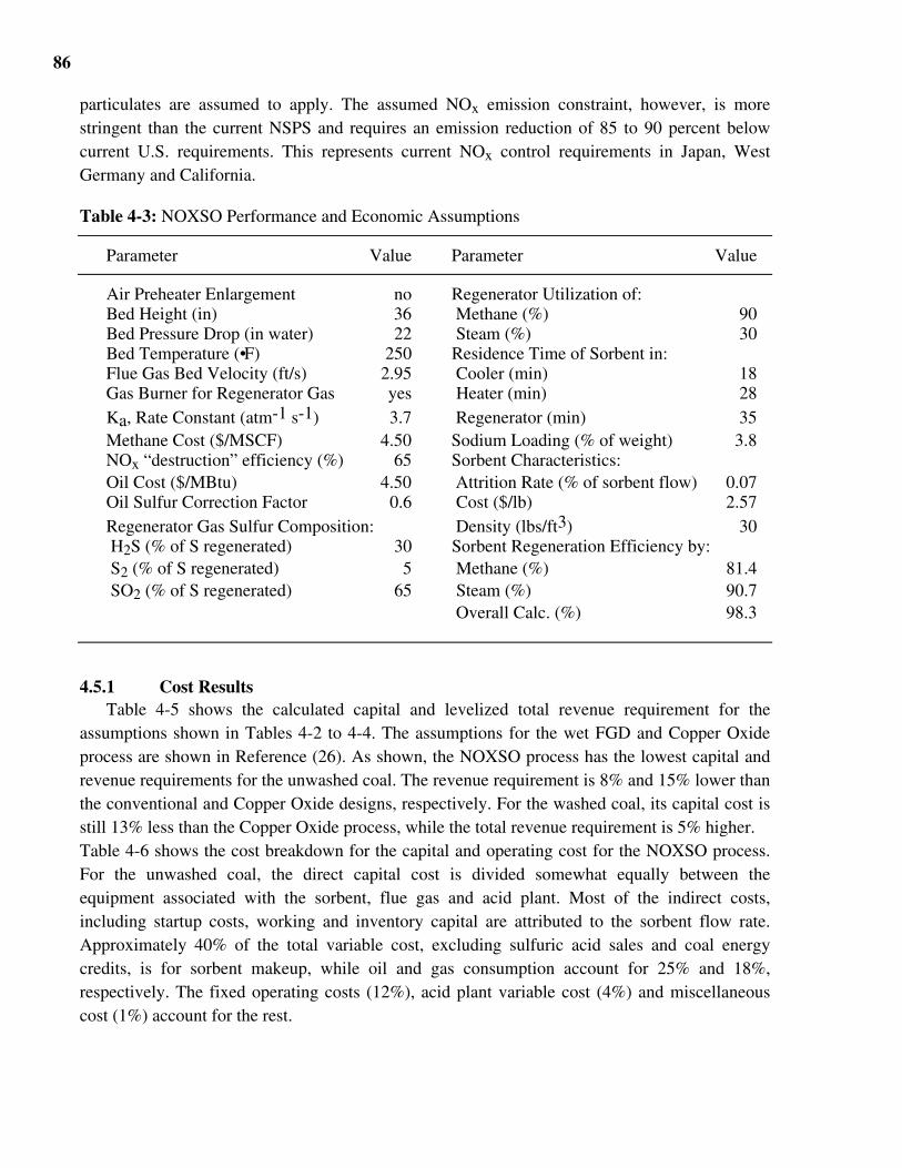
86
particulates are assumed to apply. The assumed NOx emission constraint, however, is morestringent than the current NSPS and requires an emission reduction of 85 to 90 percent belowcurrent U.S. requirements. This represents current NOx control requirements in Japan, WestGermany and California.
Table 4-3: NOXSO Performance and Economic Assumptions
Parameter Value Parameter Value
Air Preheater Enlargement no Regenerator Utilization of:Bed Height (in) 36 Methane (%) 90Bed Pressure Drop (in water) 22 Steam (%) 30Bed Temperature (•F) 250 Residence Time of Sorbent in:Flue Gas Bed Velocity (ft/s) 2.95 Cooler (min) 18Gas Burner for Regenerator Gas yes Heater (min) 28Ka, Rate Constant (atm-1 s-1) 3.7 Regenerator (min) 35Methane Cost ($/MSCF) 4.50 Sodium Loading (% of weight) 3.8NOx “destruction” efficiency (%) 65 Sorbent Characteristics:Oil Cost ($/MBtu) 4.50 Attrition Rate (% of sorbent flow) 0.07Oil Sulfur Correction Factor 0.6 Cost ($/lb) 2.57Regenerator Gas Sulfur Composition: Density (lbs/ft3) 30 H2S (% of S regenerated) 30 Sorbent Regeneration Efficiency by: S2 (% of S regenerated) 5 Methane (%) 81.4 SO2 (% of S regenerated) 65 Steam (%) 90.7
Overall Calc. (%) 98.3
4.5.1 Cost ResultsTable 4-5 shows the calculated capital and levelized total revenue requirement for the
assumptions shown in Tables 4-2 to 4-4. The assumptions for the wet FGD and Copper Oxideprocess are shown in Reference (26). As shown, the NOXSO process has the lowest capital andrevenue requirements for the unwashed coal. The revenue requirement is 8% and 15% lower thanthe conventional and Copper Oxide designs, respectively. For the washed coal, its capital cost isstill 13% less than the Copper Oxide process, while the total revenue requirement is 5% higher.Table 4-6 shows the cost breakdown for the capital and operating cost for the NOXSO process.For the unwashed coal, the direct capital cost is divided somewhat equally between theequipment associated with the sorbent, flue gas and acid plant. Most of the indirect costs,including startup costs, working and inventory capital are attributed to the sorbent flow rate.Approximately 40% of the total variable cost, excluding sulfuric acid sales and coal energycredits, is for sorbent makeup, while oil and gas consumption account for 25% and 18%,respectively. The fixed operating costs (12%), acid plant variable cost (4%) and miscellaneouscost (1%) account for the rest.
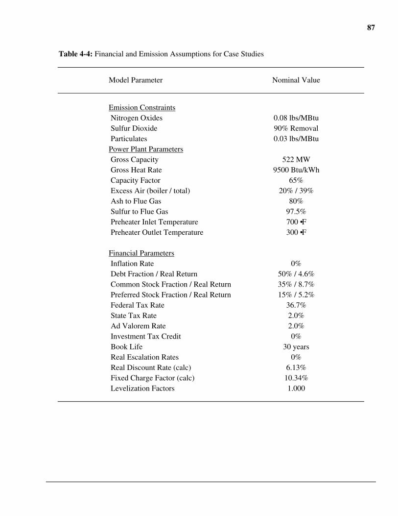
87
Table 4-4: Financial and Emission Assumptions for Case Studies
Model Parameter Nominal Value
Emission Constraints Nitrogen Oxides 0.08 lbs/MBtu Sulfur Dioxide 90% Removal Particulates 0.03 lbs/MBtuPower Plant Parameters Gross Capacity 522 MW Gross Heat Rate 9500 Btu/kWh Capacity Factor 65% Excess Air (boiler / total) 20% / 39% Ash to Flue Gas 80% Sulfur to Flue Gas 97.5% Preheater Inlet Temperature 700 •F Preheater Outlet Temperature 300 •F
Financial Parameters Inflation Rate 0% Debt Fraction / Real Return 50% / 4.6% Common Stock Fraction / Real Return 35% / 8.7% Preferred Stock Fraction / Real Return 15% / 5.2% Federal Tax Rate 36.7% State Tax Rate 2.0% Ad Valorem Rate 2.0% Investment Tax Credit 0% Book Life 30 years Real Escalation Rates 0% Real Discount Rate (calc) 6.13% Fixed Charge Factor (calc) 10.34% Levelization Factors 1.000
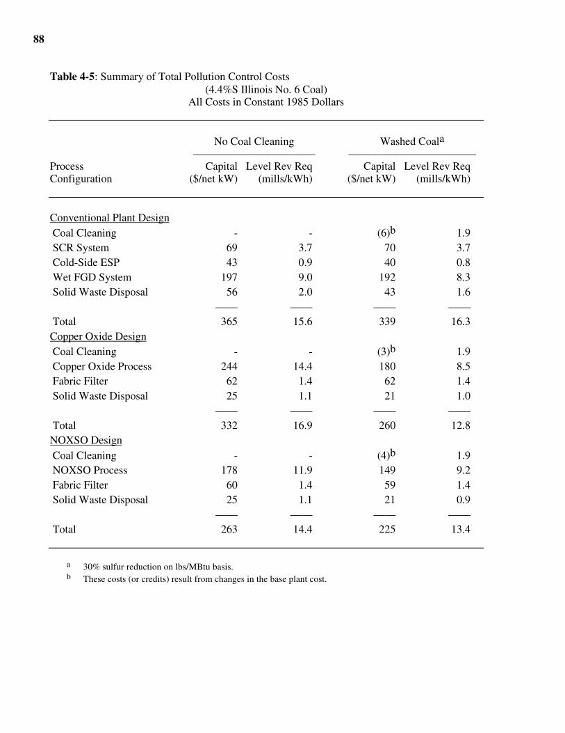
88
Table 4-5: Summary of Total Pollution Control Costs(4.4%S Illinois No. 6 Coal)
All Costs in Constant 1985 Dollars
No Coal Cleaning Washed Coala—————–—–———— ————–———————
Process Capital Level Rev Req Capital Level Rev ReqConfiguration ($/net kW) (mills/kWh) ($/net kW) (mills/kWh)
Conventional Plant Design Coal Cleaning - - (6)b 1.9 SCR System 69 3.7 70 3.7 Cold-Side ESP 43 0.9 40 0.8 Wet FGD System 197 9.0 192 8.3 Solid Waste Disposal 56 2.0 43 1.6 —— —— —— —— Total 365 15.6 339 16.3Copper Oxide Design Coal Cleaning - - (3)b 1.9 Copper Oxide Process 244 14.4 180 8.5 Fabric Filter 62 1.4 62 1.4 Solid Waste Disposal 25 1.1 21 1.0
—— —— —— —— Total 332 16.9 260 12.8NOXSO Design Coal Cleaning - - (4)b 1.9 NOXSO Process 178 11.9 149 9.2 Fabric Filter 60 1.4 59 1.4 Solid Waste Disposal 25 1.1 21 0.9
—— —— —— —— Total 263 14.4 225 13.4
a 30% sulfur reduction on lbs/MBtu basis.b These costs (or credits) result from changes in the base plant cost.
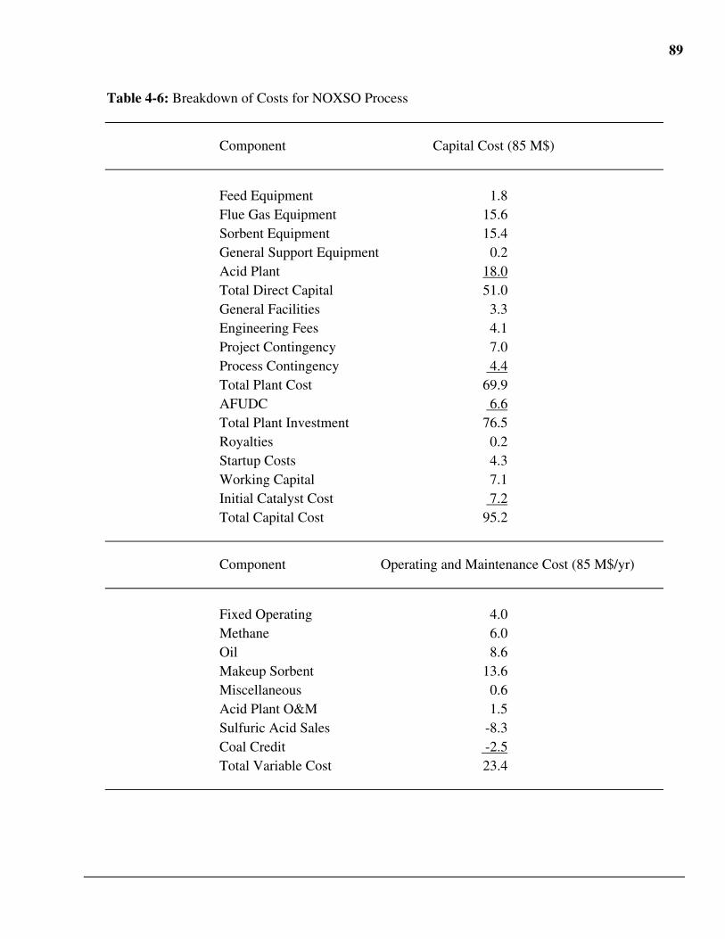
89
Table 4-6: Breakdown of Costs for NOXSO Process
Component Capital Cost (85 M$)
Feed Equipment 1.8Flue Gas Equipment 15.6Sorbent Equipment 15.4General Support Equipment 0.2Acid Plant 18.0Total Direct Capital 51.0General Facilities 3.3Engineering Fees 4.1Project Contingency 7.0Process Contingency 4.4Total Plant Cost 69.9AFUDC 6.6Total Plant Investment 76.5Royalties 0.2Startup Costs 4.3Working Capital 7.1Initial Catalyst Cost 7.2Total Capital Cost 95.2
Component Operating and Maintenance Cost (85 M$/yr)
Fixed Operating 4.0Methane 6.0Oil 8.6Makeup Sorbent 13.6Miscellaneous 0.6Acid Plant O&M 1.5Sulfuric Acid Sales -8.3Coal Credit -2.5Total Variable Cost 23.4
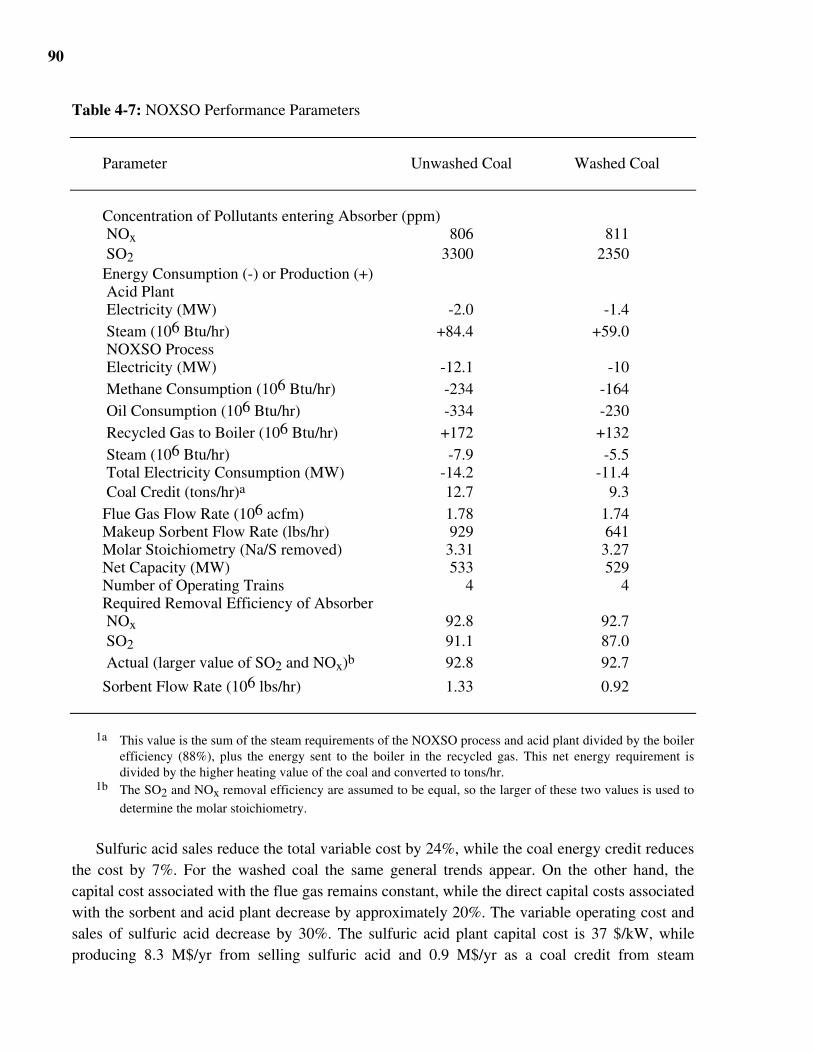
90
Table 4-7: NOXSO Performance Parameters
Parameter Unwashed Coal Washed Coal
Concentration of Pollutants entering Absorber (ppm) NOx 806 811 SO2 3300 2350Energy Consumption (-) or Production (+) Acid Plant Electricity (MW) -2.0 -1.4 Steam (106 Btu/hr) +84.4 +59.0 NOXSO Process Electricity (MW) -12.1 -10 Methane Consumption (106 Btu/hr) -234 -164 Oil Consumption (106 Btu/hr) -334 -230 Recycled Gas to Boiler (106 Btu/hr) +172 +132 Steam (106 Btu/hr) -7.9 -5.5 Total Electricity Consumption (MW) -14.2 -11.4 Coal Credit (tons/hr)a 12.7 9.3Flue Gas Flow Rate (106 acfm) 1.78 1.74Makeup Sorbent Flow Rate (lbs/hr) 929 641Molar Stoichiometry (Na/S removed) 3.31 3.27Net Capacity (MW) 533 529Number of Operating Trains 4 4Required Removal Efficiency of Absorber NOx 92.8 92.7 SO2 91.1 87.0 Actual (larger value of SO2 and NOx)b 92.8 92.7
Sorbent Flow Rate (106 lbs/hr) 1.33 0.92
1a This value is the sum of the steam requirements of the NOXSO process and acid plant divided by the boilerefficiency (88%), plus the energy sent to the boiler in the recycled gas. This net energy requirement isdivided by the higher heating value of the coal and converted to tons/hr.
1b The SO2 and NOx removal efficiency are assumed to be equal, so the larger of these two values is used to
determine the molar stoichiometry.
Sulfuric acid sales reduce the total variable cost by 24%, while the coal energy credit reducesthe cost by 7%. For the washed coal the same general trends appear. On the other hand, thecapital cost associated with the flue gas remains constant, while the direct capital costs associatedwith the sorbent and acid plant decrease by approximately 20%. The variable operating cost andsales of sulfuric acid decrease by 30%. The sulfuric acid plant capital cost is 37 $/kW, whileproducing 8.3 M$/yr from selling sulfuric acid and 0.9 M$/yr as a coal credit from steam
91
production. The variable and utility cost is 2.1 M$/yr. This translates into a savings of 1.7mills/kWh for the NOXSO process or a profit of 31 $/ton for the sulfuric acid generated. For thewashed coal, the capital cost is 30 $/kW and the sulfuric acid sales are 5.8 M$/yr. The net resultis a savings of 1.1 mills/kWh or 28 $/ton.
4.5.2 NOx Removal EfficiencyOriginally, NOXSO believed that the NOx removal efficiency was a function of the SO2
concentration and the bed temperature (20). In Reference (1), it was estimated that at a bedtemperature of 248•F the NOx and SO2 removal efficiencies would be equal. However, in theprocess developmental unit test at the Pittsburgh Energy Technology Center (PETC), theexperimental data did not show any clear correlation between NOx removal efficiency and bedtemperature (27). However, there was clear evidence that the NOx removal efficiency wasdepended on the regeneration gas. Methane was found to improve the NOx removal efficiencycompared to hydrogen. Four experimental tests were conducted using methane at a bedtemperature of approximately 245•F. The SO2 and NOx concentrations were held atapproximately 2300 and 630 ppm, respectively. Three test were conducted at an 18 inch bedheight, the other was at 42 inches. For three of the tests with removal efficiencies were greaterthan 84%, the SO2 and NOx removal efficiencies were within + 2. For the other test, the removalefficiencies were much lower (SO2 equalled 69%, while NOx equalled 78%). For the reasonsshown above the SO2 and NOx removal efficiencies are assumed to be equalled.
In Reference (27), NOXSO also showed that the NOx removal efficiency was correlated tothe ratio of SO2 to NOx by a factor of 0.80. However, all the data came from experiments whichused hydrogen as a regeneration gas and it is not clear if the same trend would hold if methane isused as a regeneration gas. NOXSO also showed a significant transient effect of increasing theratio of SO2 to NOx from 3.1 to 4.1. The steady-state effect was small, approximately 3.5removal points. Since this is a steady-state model, the transient change is not useful. Yet, it couldbe very useful to a power plant operator. These test were also conducted using hydrogen, so thesteady-state effect may not be applicable using methane—especially if removal efficiencies of90% or greater are required.
4.5.3 Effects of StoichiometryTable 4-7 gives a breakdown of the important performance parameters for the washed and
unwashed coals. For both cases the required NOx removal efficiency, (92.8%) is higher than theSO2 efficiency, (91.1%). This is caused by the inefficient destruction of NOx which is recycledto the boiler. Since the NOx and SO2 efficiencies are assumed to be equal, the molarstoichiometry is determined by the NOx removal efficiency. As shown, the sorbent flow ratedecreases by 30% for the washed coal. However, if the molar stoichiometry was driven by theSO2 removal efficiency, its value for the unwashed and washed coals would be 2.8 and 2.2respectively, instead of 3.3. These stoichiometries would produce sorbent flow rates of 1.1 x 10⁶
lbs/hr and 0.57 x 10⁶ lbs/hr, respectively. The NOXSO process capital cost would decrease from178 to 166 $/kW for the unwashed coal and from 149 to 129 $/kW for the washed and the totalNOXSO process revenue requirement would fall to 10.4 mills/kWh and 6.8 mills/kWh,respectively. Thus, if the NOx “destruction” efficiency was improved substantially or the NOx
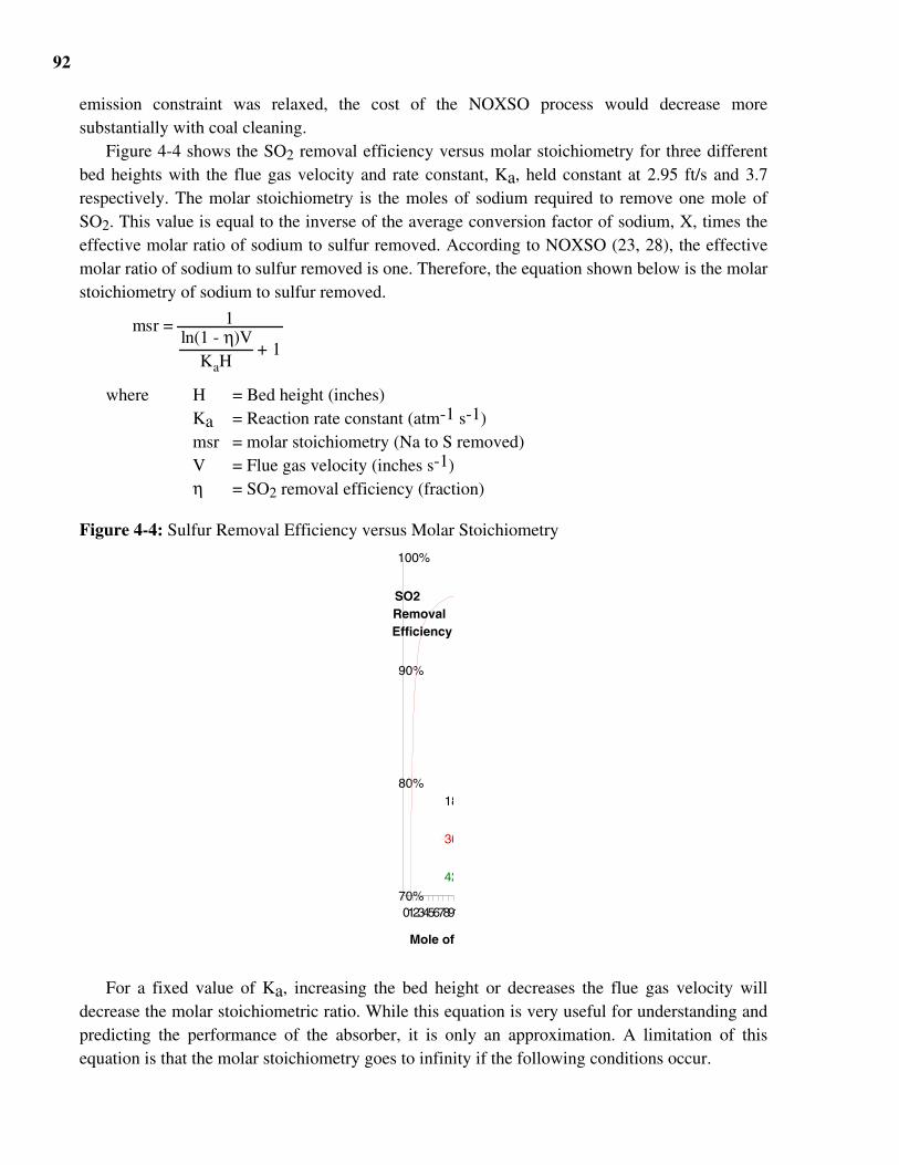
92
emission constraint was relaxed, the cost of the NOXSO process would decrease moresubstantially with coal cleaning.
Figure 4-4 shows the SO2 removal efficiency versus molar stoichiometry for three differentbed heights with the flue gas velocity and rate constant, Ka, held constant at 2.95 ft/s and 3.7respectively. The molar stoichiometry is the moles of sodium required to remove one mole ofSO2. This value is equal to the inverse of the average conversion factor of sodium, X, times theeffective molar ratio of sodium to sulfur removed. According to NOXSO (23, 28), the effectivemolar ratio of sodium to sulfur removed is one. Therefore, the equation shown below is the molarstoichiometry of sodium to sulfur removed.
msr =
KaHln(1 - η)V
+ 1
1
where H = Bed height (inches)Ka = Reaction rate constant (atm-1 s-1)msr = molar stoichiometry (Na to S removed)V = Flue gas velocity (inches s-1)η = SO2 removal efficiency (fraction)
Figure 4-4: Sulfur Removal Efficiency versus Molar Stoichiometry
70%
80%
90%
100%
01234567891
SO2RemovalEfficiency
18
36
42
Mole of
For a fixed value of Ka, increasing the bed height or decreases the flue gas velocity willdecrease the molar stoichiometric ratio. While this equation is very useful for understanding andpredicting the performance of the absorber, it is only an approximation. A limitation of thisequation is that the molar stoichiometry goes to infinity if the following conditions occur.
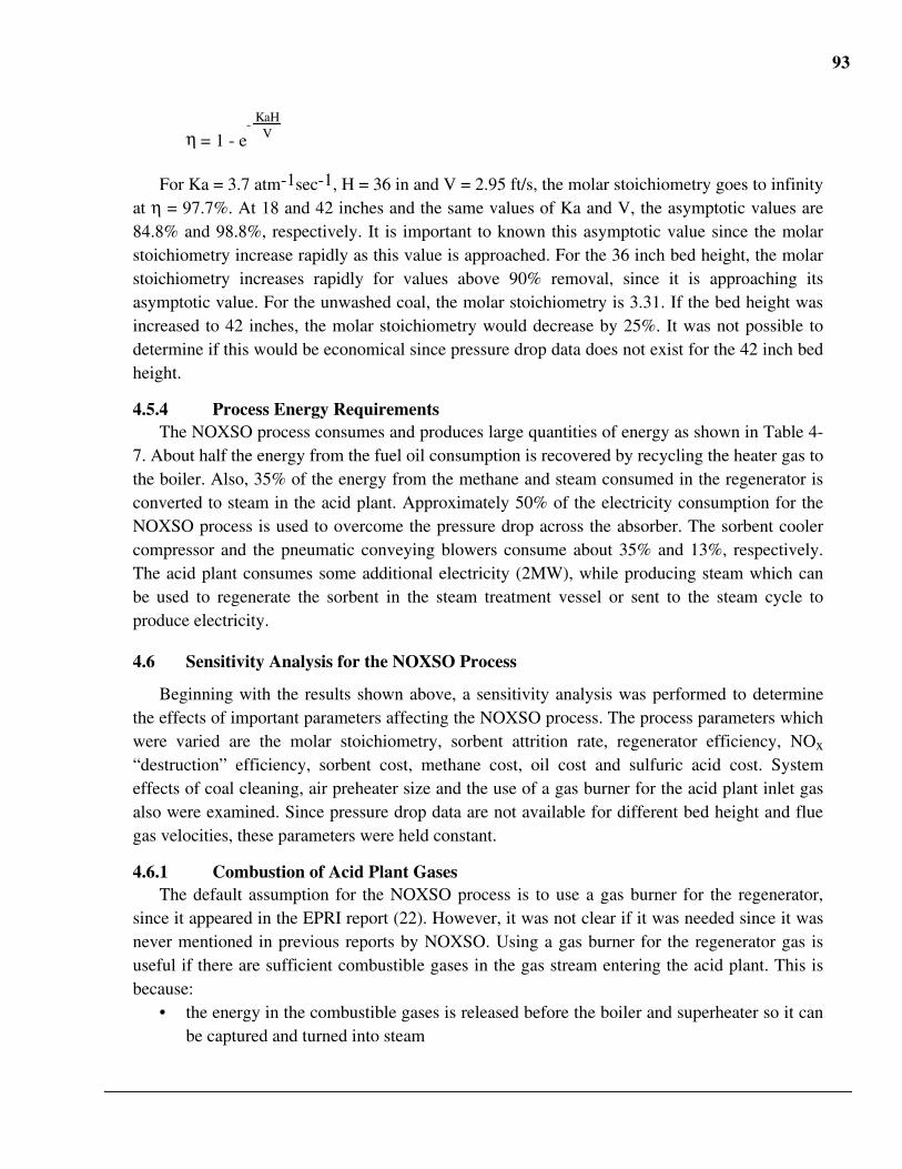
93
η = 1 - e-
VKaH
For Ka = 3.7 atm-1sec-1, H = 36 in and V = 2.95 ft/s, the molar stoichiometry goes to infinityat η = 97.7%. At 18 and 42 inches and the same values of Ka and V, the asymptotic values are84.8% and 98.8%, respectively. It is important to known this asymptotic value since the molarstoichiometry increase rapidly as this value is approached. For the 36 inch bed height, the molarstoichiometry increases rapidly for values above 90% removal, since it is approaching itsasymptotic value. For the unwashed coal, the molar stoichiometry is 3.31. If the bed height wasincreased to 42 inches, the molar stoichiometry would decrease by 25%. It was not possible todetermine if this would be economical since pressure drop data does not exist for the 42 inch bedheight.
4.5.4 Process Energy RequirementsThe NOXSO process consumes and produces large quantities of energy as shown in Table 4-
7. About half the energy from the fuel oil consumption is recovered by recycling the heater gas tothe boiler. Also, 35% of the energy from the methane and steam consumed in the regenerator isconverted to steam in the acid plant. Approximately 50% of the electricity consumption for theNOXSO process is used to overcome the pressure drop across the absorber. The sorbent coolercompressor and the pneumatic conveying blowers consume about 35% and 13%, respectively.The acid plant consumes some additional electricity (2MW), while producing steam which canbe used to regenerate the sorbent in the steam treatment vessel or sent to the steam cycle toproduce electricity.
4.6 Sensitivity Analysis for the NOXSO Process
Beginning with the results shown above, a sensitivity analysis was performed to determinethe effects of important parameters affecting the NOXSO process. The process parameters whichwere varied are the molar stoichiometry, sorbent attrition rate, regenerator efficiency, NOx
“destruction” efficiency, sorbent cost, methane cost, oil cost and sulfuric acid cost. Systemeffects of coal cleaning, air preheater size and the use of a gas burner for the acid plant inlet gasalso were examined. Since pressure drop data are not available for different bed height and fluegas velocities, these parameters were held constant.
4.6.1 Combustion of Acid Plant GasesThe default assumption for the NOXSO process is to use a gas burner for the regenerator,
since it appeared in the EPRI report (22). However, it was not clear if it was needed since it wasnever mentioned in previous reports by NOXSO. Using a gas burner for the regenerator gas isuseful if there are sufficient combustible gases in the gas stream entering the acid plant. This isbecause:
• the energy in the combustible gases is released before the boiler and superheater so it canbe captured and turned into steam
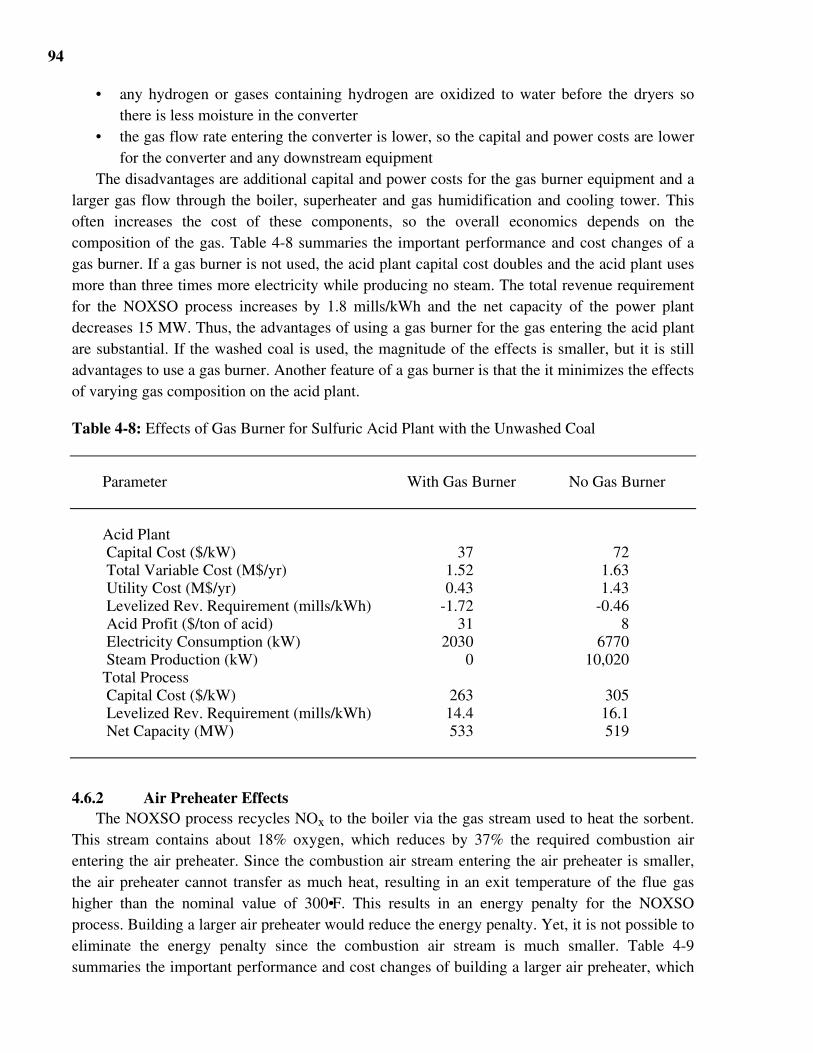
94
• any hydrogen or gases containing hydrogen are oxidized to water before the dryers sothere is less moisture in the converter
• the gas flow rate entering the converter is lower, so the capital and power costs are lowerfor the converter and any downstream equipment
The disadvantages are additional capital and power costs for the gas burner equipment and alarger gas flow through the boiler, superheater and gas humidification and cooling tower. Thisoften increases the cost of these components, so the overall economics depends on thecomposition of the gas. Table 4-8 summaries the important performance and cost changes of agas burner. If a gas burner is not used, the acid plant capital cost doubles and the acid plant usesmore than three times more electricity while producing no steam. The total revenue requirementfor the NOXSO process increases by 1.8 mills/kWh and the net capacity of the power plantdecreases 15 MW. Thus, the advantages of using a gas burner for the gas entering the acid plantare substantial. If the washed coal is used, the magnitude of the effects is smaller, but it is stilladvantages to use a gas burner. Another feature of a gas burner is that the it minimizes the effectsof varying gas composition on the acid plant.
Table 4-8: Effects of Gas Burner for Sulfuric Acid Plant with the Unwashed Coal
Parameter With Gas Burner No Gas Burner
Acid Plant Capital Cost ($/kW) 37 72 Total Variable Cost (M$/yr) 1.52 1.63 Utility Cost (M$/yr) 0.43 1.43 Levelized Rev. Requirement (mills/kWh) -1.72 -0.46 Acid Profit ($/ton of acid) 31 8 Electricity Consumption (kW) 2030 6770 Steam Production (kW) 0 10,020Total Process Capital Cost ($/kW) 263 305 Levelized Rev. Requirement (mills/kWh) 14.4 16.1 Net Capacity (MW) 533 519
4.6.2 Air Preheater EffectsThe NOXSO process recycles NOx to the boiler via the gas stream used to heat the sorbent.
This stream contains about 18% oxygen, which reduces by 37% the required combustion airentering the air preheater. Since the combustion air stream entering the air preheater is smaller,the air preheater cannot transfer as much heat, resulting in an exit temperature of the flue gashigher than the nominal value of 300•F. This results in an energy penalty for the NOXSOprocess. Building a larger air preheater would reduce the energy penalty. Yet, it is not possible toeliminate the energy penalty since the combustion air stream is much smaller. Table 4-9summaries the important performance and cost changes of building a larger air preheater, which
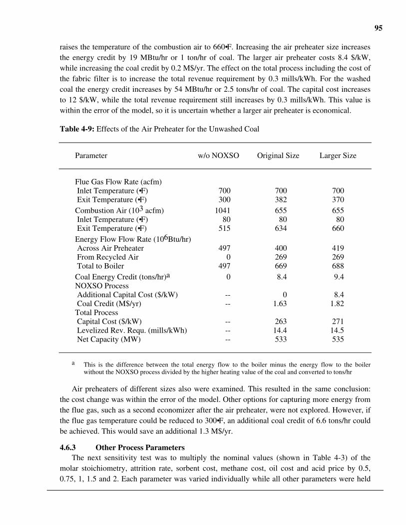
95
raises the temperature of the combustion air to 660•F. Increasing the air preheater size increasesthe energy credit by 19 MBtu/hr or 1 ton/hr of coal. The larger air preheater costs 8.4 $/kW,while increasing the coal credit by 0.2 M$/yr. The effect on the total process including the cost ofthe fabric filter is to increase the total revenue requirement by 0.3 mills/kWh. For the washedcoal the energy credit increases by 54 MBtu/hr or 2.5 tons/hr of coal. The capital cost increasesto 12 $/kW, while the total revenue requirement still increases by 0.3 mills/kWh. This value iswithin the error of the model, so it is uncertain whether a larger air preheater is economical.
Table 4-9: Effects of the Air Preheater for the Unwashed Coal
Parameter w/o NOXSO Original Size Larger Size
Flue Gas Flow Rate (acfm) Inlet Temperature (•F) 700 700 700 Exit Temperature (•F) 300 382 370Combustion Air (103 acfm) 1041 655 655 Inlet Temperature (•F) 80 80 80 Exit Temperature (•F) 515 634 660Energy Flow Flow Rate (106Btu/hr) Across Air Preheater 497 400 419 From Recycled Air 0 269 269 Total to Boiler 497 669 688Coal Energy Credit (tons/hr)a 0 8.4 9.4NOXSO Process Additional Capital Cost ($/kW) -- 0 8.4 Coal Credit (M$/yr) -- 1.63 1.82Total Process Capital Cost ($/kW) -- 263 271 Levelized Rev. Requ. (mills/kWh) -- 14.4 14.5 Net Capacity (MW) -- 533 535
a This is the difference between the total energy flow to the boiler minus the energy flow to the boilerwithout the NOXSO process divided by the higher heating value of the coal and converted to tons/hr
Air preheaters of different sizes also were examined. This resulted in the same conclusion:the cost change was within the error of the model. Other options for capturing more energy fromthe flue gas, such as a second economizer after the air preheater, were not explored. However, ifthe flue gas temperature could be reduced to 300•F, an additional coal credit of 6.6 tons/hr couldbe achieved. This would save an additional 1.3 M$/yr.
4.6.3 Other Process ParametersThe next sensitivity test was to multiply the nominal values (shown in Table 4-3) of the
molar stoichiometry, attrition rate, sorbent cost, methane cost, oil cost and acid price by 0.5,0.75, 1, 1.5 and 2. Each parameter was varied individually while all other parameters were held
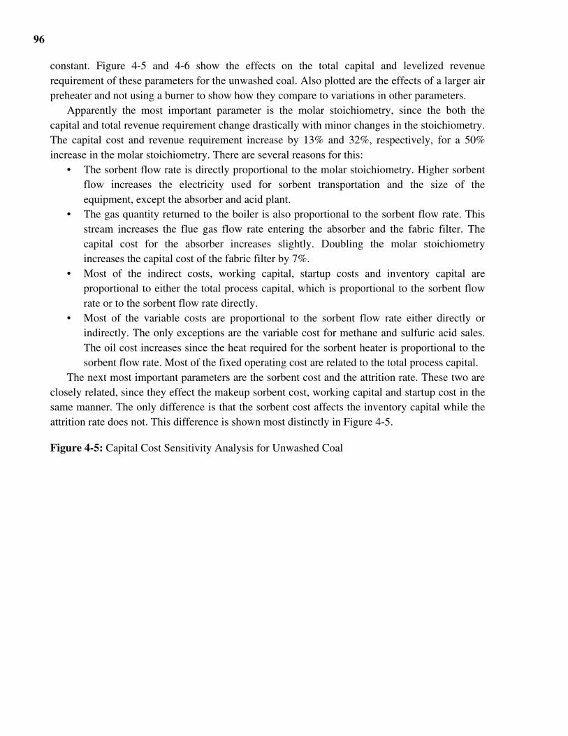
96
constant. Figure 4-5 and 4-6 show the effects on the total capital and levelized revenuerequirement of these parameters for the unwashed coal. Also plotted are the effects of a larger airpreheater and not using a burner to show how they compare to variations in other parameters.
Apparently the most important parameter is the molar stoichiometry, since the both thecapital and total revenue requirement change drastically with minor changes in the stoichiometry.The capital cost and revenue requirement increase by 13% and 32%, respectively, for a 50%increase in the molar stoichiometry. There are several reasons for this:
• The sorbent flow rate is directly proportional to the molar stoichiometry. Higher sorbentflow increases the electricity used for sorbent transportation and the size of theequipment, except the absorber and acid plant.
• The gas quantity returned to the boiler is also proportional to the sorbent flow rate. Thisstream increases the flue gas flow rate entering the absorber and the fabric filter. Thecapital cost for the absorber increases slightly. Doubling the molar stoichiometryincreases the capital cost of the fabric filter by 7%.
• Most of the indirect costs, working capital, startup costs and inventory capital areproportional to either the total process capital, which is proportional to the sorbent flowrate or to the sorbent flow rate directly.
• Most of the variable costs are proportional to the sorbent flow rate either directly orindirectly. The only exceptions are the variable cost for methane and sulfuric acid sales.The oil cost increases since the heat required for the sorbent heater is proportional to thesorbent flow rate. Most of the fixed operating cost are related to the total process capital.
The next most important parameters are the sorbent cost and the attrition rate. These two areclosely related, since they effect the makeup sorbent cost, working capital and startup cost in thesame manner. The only difference is that the sorbent cost affects the inventory capital while theattrition rate does not. This difference is shown most distinctly in Figure 4-5.
Figure 4-5: Capital Cost Sensitivity Analysis for Unwashed Coal
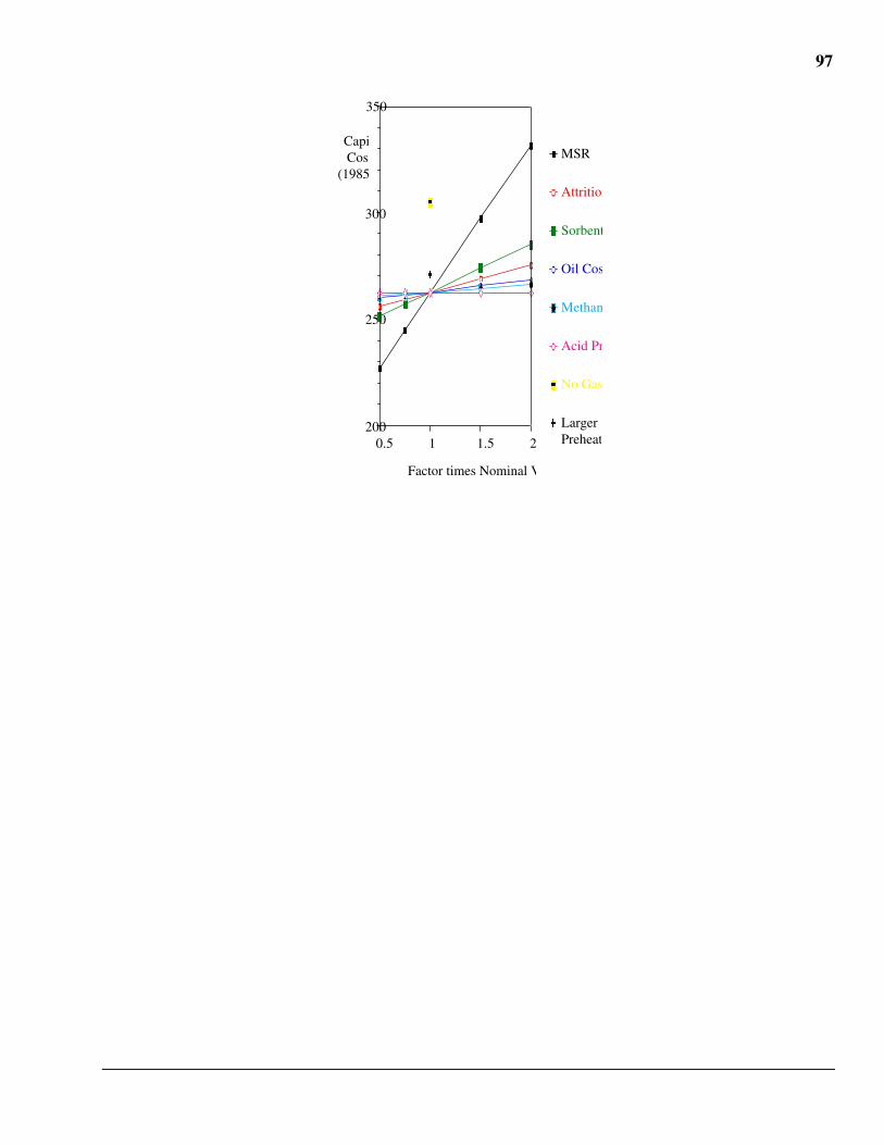
97
MSR
Attrition
Sorbent
Oil Cos
Methan
Acid Pr
No Gas
Larger APreheat
200
250
300
350
0.5 1 1.5 2
Factor times Nominal V
CapiCost
(1985
98
Figure 4-6: Total Revenue Requirement Sensitivity Analysis
Levelized Revenue
Requirement (1985mills/kWh)
MSR
Attrition
Sorbent Cost
Oil Cost
Methane Cost
Acid Price
No Gas Burner
Larger Air Preheater
10
15
20
25
0.5 1 1.5 2
Factor times Nominal Value of Parameter
Of the remaining parameters, the price of methane, fuel oil and sulfuric acid, the totalrevenue requirement is most sensitive to the price of oil and least sensitive to the price ofmethane. A 50% increase in the price of oil increases the total revenue requirement by 10%,while the same increase in methane cost, results in a 7% increase. These two parameters alsoaffect the capital cost since they affect the startup and working capital. The price of sulfuric acidhas no effect on the capital cost, while having a significant effect on the total revenuerequirement. A 50% increase in the price of sulfuric acid decreases the total revenue requirementby 8.5%.
4.6.4 NOx Reduction EfficiencyFigure 4-7 shows the capital and revenue requirements for different values of the NOx being
destroyed in the boiler. The NOx “destruction” efficiency determines the NOx removal efficiencyrequired in the adsorber to meet the emission standard. As this value decreases the removalefficiency increases since there is a more NOx entering the adsorber. Between destructionefficiencies of 50% and 80%, the NOx removal efficiency in the adsorber is higher than therequired SO2 removal efficiency, so any change in this parameter changes the molarstoichiometry, which has a significant effect on the overall cost. Above a NOx “destruction”efficiency of 80% the SO2 removal efficiency is greater, so the molar stoichiometry is notaffected. For the washed coal, the NOx removal efficiency is always greater so the cost alwaysdecreases with improvements in the destruction efficiency.
4.6.5 Sorbent Regenerator EfficiencyFigure 4-8 shows the capital and revenue requirements versus the overall regeneration
efficiency. The overall regeneration efficiency is a function of the efficiencies of both theregenerator and the steam treatment vessel:
ηR&S = ηR + (1 - ηR)ηSTV
whereηR the efficiency of removing sulfur from the sorbent with methane in theηSTV the efficiency of removing sulfur from the sorbent with steam in the steam
treatment vesselηR&S the overall regeneration efficiency of both vessels
99
To analyze the sensitivity of the NOXSO process to the overall regeneration efficiency, ηR
and ηSTV were given the following values: 55%, 60%, 70%, 80%, 90%, 95%. This produced theoverall efficiencies of 79.75%, 84%, 91%, 96%, 99% and 99.75% shown plotted in Figure 4-8.The nominal value is 98.27%, which was estimated from an EPRI report (22). The utilization ofmethane and steam was assumed to remain constant at their nominal values of 90% and 30%,respectively. The efficiency of the regenerator using methane was not set to 50%, because thiswould have created a gas composition which the acid plant was not designed to handle.14 Asshown, the capital and revenue requirement cannot be improved significantly, since the nominalvalue for the regeneration efficiency is high. However, if the regeneration efficiency drops to91%, then the capital and revenue requirement increase by 2.7% and 6.7%, respectively.
4.7 Conclusion
From this analysis it is obvious that the most significant parameter affecting the design andcost of the NOXSO process is the sorbent flow rate needed to achieve a given removalefficiency. Therefore, the relationship between NOx and SO2 removal efficiencies, the molarstoichiometry and regeneration process should be studied further, since they affect the sorbentflow rate directly and have a high degree of uncertainty. Data on NOx removal and destruction inthe boiler is the most critical, since it is the most uncertain of any of the parameters. Moreexperimental data is needed to confirm the analytical model for SO2 removal efficiency.However, the results of the performance model are consistent with previous studies.
Experiments using a continuous regenerator should be performed since only batch test havebeen performed. These experiments should be designed to develop a performance curve relatingmethane and steam consumption to regeneration efficiency and predict the regenerated gascomposition. If a performance curve existed, the IEC model could be used to optimize theNOXSO process, since the tradeoffs between the sorbent flow rate, oil consumption, methaneconsumption and acid plant are modeled explicitly.
The analysis of the air preheater showed that an additional that an energy credit worth 1.3M$/yr can be achieved if the temperature in the flue gas is reduced to 300•F. Other options forcapturing this energy should be explored. A second economizer after the air preheater may beeconomical.
Figure 4-7: Effect of NOx Destruction Efficiency in Boiler
14 The inlet sulfur dioxide concentration was too low for this design, so the capital and operating cost would not
be valid.
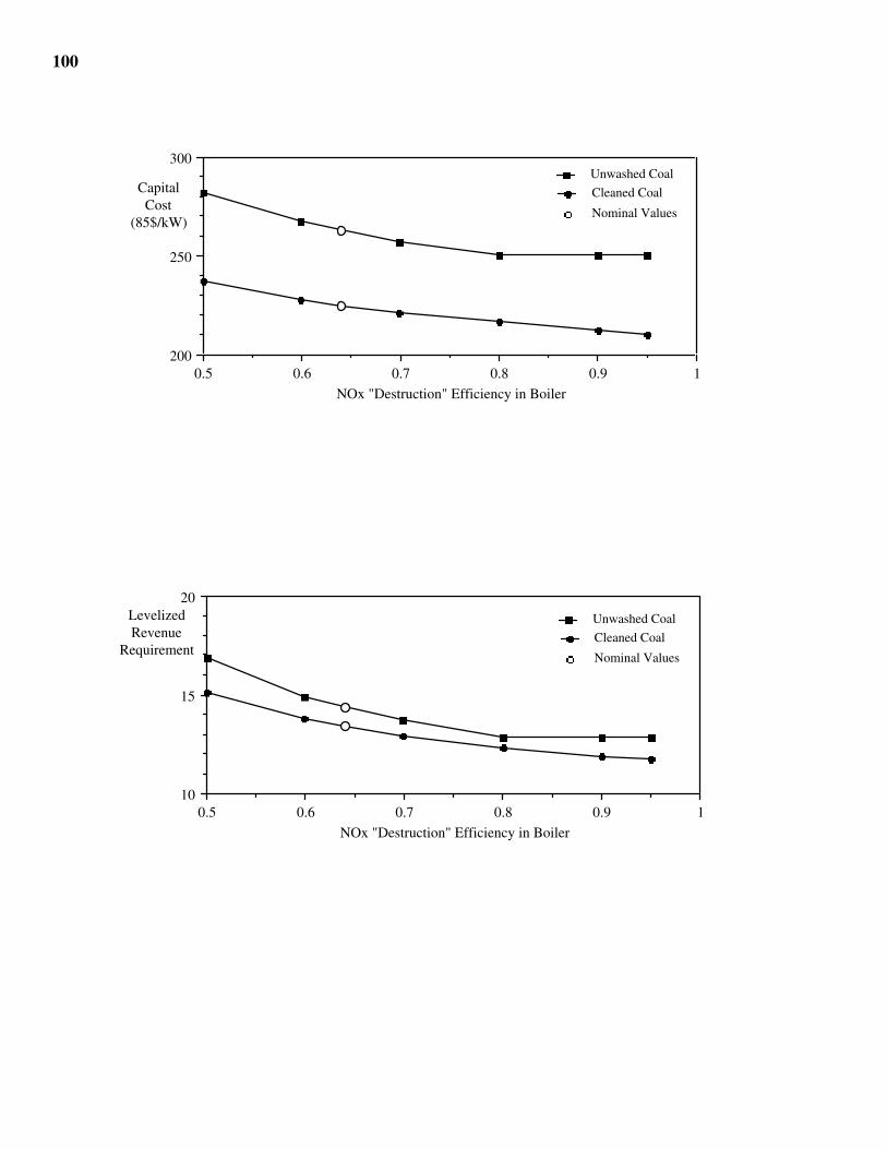
100
Capital Cost
(85$/kW)
200
250
300
0.5 0.6 0.7 0.8 0.9 1
NOx "Destruction" Efficiency in Boiler
Unwashed Coal
Cleaned Coal
Nominal Values
10
15
20
0.5 0.6 0.7 0.8 0.9 1
Levelized Revenue
Requirement
NOx "Destruction" Efficiency in Boiler
Unwashed Coal
Cleaned Coal
Nominal Values
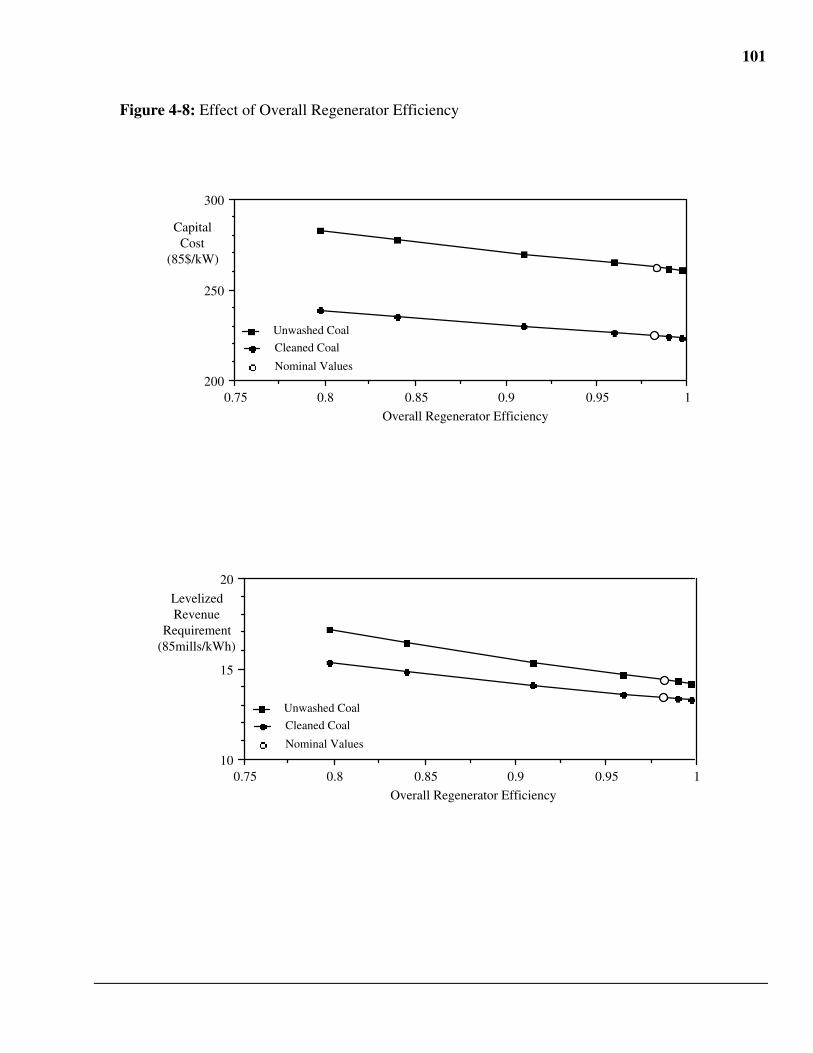
101
Figure 4-8: Effect of Overall Regenerator Efficiency
Unwashed Coal
Cleaned Coal
Nominal Values200
250
300
0.75 0.8 0.85 0.9 0.95 1
Overall Regenerator Efficiency
Capital Cost
(85$/kW)
Levelized Revenue
Requirement (85mills/kWh)
10
15
20
0.75 0.8 0.85 0.9 0.95 1
Overall Regenerator Efficiency
Unwashed Coal
Cleaned Coal
Nominal Values
102
5 ELECTRON BEAM PROCESS MODEL
5.1 Nomenclature
English SymbolsByp Bypass (fraction)Cj Concentration of j in flue gas (ppm)D Electron beam dosage (Mrads)ES Emission standard (lb/million Btu into furnace)Hhv Higher heating value of fuel (Btu/lb)m#,j Molar flow rate of component j at point # (lb•mole/hr)M#,j Mass flow rate of component j at point # (tons/hr)Rpurity Purity of reagent (fraction)T# Temperature at point # (•R)
Greek Symbols∆T Temperature difference (•F)η Efficiency (fraction)σ Molar stoichiometry (fraction)
Subcategories for Combustion Air and Flue Gas ComponentsCO Carbon monoxideCO2 Carbon dioxideH2O MoistureN2 NitrogenNO Nitrogen oxideNO2 Nitrogen dioxideO2 OxygenSO2 Sulfur dioxideSO3 Sulfur trioxide
Subcategories for Solid Stream ComponentsAsh AshCaO LimeCaCO3 LimestoneCaSO3•.5H2O Hydrated calcium sulfiteCaSO4 Calcium SulfateCaSO4•2H2O Hydrated calcium sulfateH2O Water or MoistureMisc Miscellaneous
General Subcategorieseb Electron beam chamberexit Exiting devicefgapho Exiting air preheater on flue gas sidefuel Fuel streamin Entering deviceNOx Nitrogen oxidesat Saturation
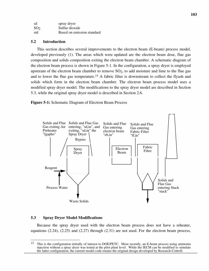
103
sd spray dryerSO2 Sulfur dioxidestd Based on emission standard
5.2 Introduction
This section describes several improvements to the electron beam (E-beam) process model,developed previously (1). The areas which were updated are the electron beam dose, flue gascomposition and solids composition exiting the electron beam chamber. A schematic diagram ofthe electron beam process is shown in Figure 5-1. In the configuration, a spray dryer is employedupstream of the electron beam chamber to remove SO2, to add moisture and lime to the flue gasand to lower the flue gas temperature.15 A fabric filter is downstream to collect the flyash andsolids which form in the electron beam chamber. The electron beam process model uses amodified spray dryer model. The modifications to the spray dryer model are described in Section5.3, while the original spray dryer model is described in Section 2.6.
Figure 5-1: Schematic Diagram of Electron Beam Process
Fabric Filter
Electron Beam
Spray Dryer
Bypass
Waste Solids
Reagent
Process Water
Solids and Flue Gas exiting Air Preheater "fgapho"
Solids and Flue Gas entering, "sd,in", and exiting, "sd,in" the Spray Dryer
Solids and Flue Gas entering electron beam "eb,in"
Solids and Flue Gas entering Fabric Filter "ff,in"
Solids and Flue Gas entering Stack "stack"
5.3 Spray Dryer Model Modifications
Because the spray dryer used with the electron beam process does not have a reheater,equations (2.24), (2.25) and (2.27) through (2.31) are not used. For the electron beam process,
15 This is the configuration initially of interest to DOE/PETC. More recently, an E-beam process using ammonia
injection without a spray dryer was tested at the pilot plant level. While the IECM can be modified to simulatethe latter configuration, the current model code retains the original design developed by Research-Cottrell.
104
the flue gas exiting the spray dryer enters the electron beam process instead of a fabric filter. Theresult of modifying equations (2.22) and (2.23) are shown below:
meb,in,j = msd,exit, j + Byp mfgapho,j
Teb,in = Byp Tfgapho + (1 - Byp) Tsd,exit
In the original spray dryer model, the reagent and molar stoichiometry was determined usingEquations (2.18) and (2.19). For the electron beam model, they are determined with the equationsbelow. The molar stoichiometry of the E-beam, σeb, is an input parameter and is the molar ratioof lime to sulfur dioxide plus one-half the NOx entering the spray dryer.
Mreag = 56.08 msd,in,SO2 + msd,in,SO3 + 0.5msd,in,NO + 0.5msd,in,NO2 σeb
2000 Rpurity
σsd = 2000 Mreag Rpurity
56.08 msd,in,SO2 + msd,in,SO3
In the spray dryer model, the amount of bypass and SO2 removal was determined usingEquations (2.16) and (2.16). For the electron beam model, the amount of bypass is an inputparameter and the SO2 removal is determined by solving Equation (2.18) for ηSO2.
ηSO2 = ln σsd - 0.025∆Tsat + 2.9
3.322
5.4 Electron Beam Dose
The sulfur dioxide and NOx removal efficiencies required for the ebeam process to meet theirrespective emission standards are determined by
ηSO2,std = 1 - 2000 ESSO2 Mfuel Hhvfuel
64.06 * 1,000,000 (meb,in,SO2 + meb,in,SO3)(5.1)
ηSO2,std = 1 - 2000 ESNOx Mfuel Hhvfuel
46.01 * 1,000,000 (meb,in,NO + meb,in,NO2)(5.2)
Helfritch and Feldman determined an algorithm for predicting the outlet concentration ofSO2 and NOx versus the dose of electron directed into the flue gas (29). Their algorithm is basedon the rates of reactions of the principal chemical reactions and experimental data and is shownbelow.16
16 In Reference (29), there is a typographical error for Equation 5.3. The constant "2.5" is typed as "0.25."
105
CSO2
CSO2,in
= exp -2.5 D1 + 0.0058 CSO2,in
(5.3)
CNOx
CNOx,in
= exp-0.12 D 1 + 0.058 CSO2,in
1 + 0.0058 CSO2,in
(5.4)
Typically when the IECM is used, the emission constraints are specified and the pollutioncontrol equipment has to meet these constraints. Therefore, Equations (5.3) and (5.4) are solvedfor the electron beam dose and the ratios of the outlet to inlet concentrations are replaced by oneminus the removal efficiencies specified in Equations (5.1) and (5.2).
DSO2 =
1 + 0.0058 CSO2,in * ln 1 - ηSO2,std
-2.5(5.5)
DNOx = 1 + 0.0058 CSO2,in * ln 1 - ηNOx,std
-0.12 1 + 0.058 CSO2,in
(5.6)
where
CSO2,in =
1,000,000 meb,in,SO2 + meb,in,SO3
meb,in,jj=1
9
Since the electron beam process has to meet both the NOx and SO2 emission constraints, thelarger dose determined by Equations (5.5) and (5.6) is used and the actual NOx and SO2 removalefficiencies are determined by the equations below. Thus,
if DSO2 • DNOx then D = DSO2 else D = DNOx
ηSO2 = 1 - exp -2.5 D1 + 0.0058 CSO2,in
ηNOx = 1 - exp
-0.12 D 1 + 0.058 CSO2,in
1 + 0.0058 CSO2,in
5.5 Flue Gas Composition
The composition of the flue gas changes in the electron beam chamber. The two mostsignificant changes are the reduction in the sulfur dioxide content and nitrogen oxide content.The sulfur dioxide and nitrogen oxide are removed from the flue gas by a complex set ofchemical reactions (29). These chemical reactions have been greatly simplified in the IECM andare shown below.
106
SO2 + CaO + 2H20 + 0.5O2 --> CaSO4•2H20 (5.7)SO3 + CaO + 2H20 --> CaSO4•2H202NO + CaO + H20 + 0.5O2 --> Ca(NO2)2•H202NO + CaO + 1.5O2 --> Ca(NO3)2
2NO2 + CaO + H20 --> Ca(NO2)2•H20 + 0.5O2
2NO2 + CaO + 0.5O2 --> Ca(NO3)2
Using these chemical reactions the composition of the flue gas exiting the electron beamchamber can be determined from a molar balance as shown below. The symbol, Ox, representsthe fraction of calcium nitrite oxidized to calcium nitrate.
meb,exit,j = meb,in,j for j = N2, CO2, CO
meb,exit,O2 = meb,in,O2
- 0.5 meb,in,SO2 ηSO2
+
(0.5 Ox+ 0.25 ) meb,in,NO + (0.5 Ox - 0.25) meb,in,NO2 ηNOx
meb,exit,H2O = meb,in,H2O - 2 meb,in,SO2 + meb,in,SO3 ηSO2 +
(1 - Ox) meb,in,NO + meb,in,NO2 ηNOx
meb,exit,SO2 = meb,in,SO2 - meb,in,SO2 ηSO2
meb,exit,SO3 = meb,in,SO3 - meb,in,SO3 ηSO2
meb,exit,NO = meb,in,NO - meb,in,NO ηNOx
meb,exit,NO2 = meb,in,NO2 - meb,in,NO2 ηNOx
5.6 Waste Composition
A major environmental flow stream emanating from the electron beam system is the streamof dry waste solids. The basic chemistry for the creation of these solids is shown in Equation(5.7). The difference in the composition and mass flow rates of electron beam waste depends onthe extent of oxidation of calcium nitrite to calcium nitrate, Ox. Other constituents of the electron
107
beam solids stream include unreacted reagent (which depends on the molar stoichiometry), inertmaterials introduced with the reagent (as dictated by the level of reagent purity) and the solidwaste from the spray dryer system. The total mass flow rate of the solids exiting the electronbeam is shown below.
Meb,exit,j = Meb,in,j for j = Ash, CaCO3, CaSO4, CaSO3•0.5H2O
Meb,exit,CaO = Meb,in,CaO - 56.082000
meb,in,SO2 + meb,in,SO3
ηSO2 +
0.5 meb,in,NO + meb,in,NO2 ηNOx
Meb,CaSO4•2H2O = Meb,in,CaSO4•2H2O + 172.17 meb,in,SO2 + meb,in,SO3 ηSO2
2000
Meb,exit,Misc = Meb,in,Misc + 150.1 (1-Ox) + 164.09 Ox 0.5 meb,in,NO + meb,in,NO2 ηNOx
2000
5.7 Economics Algorithm
The economic algorithm for the electron beam process has remained unchanged except oneitem. The single indirect charge factor for capital cost has been split into different categories ofindirect charges following the nomenclature of the TVA (see baseline plant section).
108
6 SULFURIC ACID PLANT MODEL
6.1 Nomenclature
English Letter SymbolsAk area of device, k (ft2)Ccategorie capital charges associated with startup ($)Cidx chemical engineering cost indexCo molar gas concentration of SO2 in the flue gas entering the adsorber (lb•mole/ft3)CF capacity factor of power plant (fraction)DCCk capital cost for device, k (M$)e# notation for specifying power of 10.Ej,k energy flow rate of specie, j, at device, k (lb•mole/hr)ECk electricity consumption of the device, k (kW)fmakeup attrition rate of sorbent (fraction)fj,wet air amount of specie, j, in ambient moist air (fraction)fpj,k quantity of specie, j, produced in device, k (fraction)Foil constant used to estimate amount of sulfur from oil (fraction)FOC fixed operating cost ($/yr)Gk gas flow rate for device, k (ft3/min) ∧hj,temperature molar enthalpy of specie, j, at specified temperature (Btu/lb•mole)H fluidized bed height in adsorber (ft)HHVj higher heating value of specie, j, (Btu/lb)HR heat rate of power plant (kW-Hr/MBtu)i inflation rate (fraction)Ka apparent rate constant (atm-1 sec-1)LMTDk log mean temperature difference of device, k (•F)mj mass flow of specie, j, (lbs/hr or tons/hr)Mjk molar flow rate of specie, j, for device, k (lb•mole/hr)MWg gross electrical capacity of power plant (MW)Nt initial loading of the active Na on sorbent (lb•mole/lb)NOP number of operating adsorbersNRD number of spare adsorbersOCcatagorie annual operating cost ($/yr)Qk heat load across heat exchanger device, k (Btu/hr)p interest rate (fraction)Pk pressure of the device, k (” water or atm)RTk residence time of sorbent in device, k (hours)Tsj,k temperature of specie, j, for the device, k (•F)TCC total capital cost ($)TPC total plant cost ($)TPI total plant investment ($)TDC total direct cost ($)TVC total operating and maintenance cost, sum of FOC and VOC ($/yr)Uk universal heat transfer coefficient for device, k (Btu/hr-ft2 •F)UCj unit cost of specie, j, ($/unit)Utj utilization constant for specie, j, in regenerator (fraction)V superficial velocity of flue gas through adsorber (ft/sec)VOC variable operating cost ($/yr)
109
WNa weight fraction of sodium to sorbent (fraction)X mean value of the fractional conversion of the sorbent in the entire adsorber (fraction)y molar fraction of SO2 in the flue gas (fraction)
Greek Letter SymbolsδNOx fraction of NOx returned to boiler which is destroyed (fraction)•Hk heat of reaction in device, k (Btu/hr)ηj,k efficiency of device, k (fraction)λ molar stoichiometry of SO2 to active sorbentρsorb bulk density of sorbent (lbs/ft3)
Subscripts1 specifies the first part or half a device, kguess used to indicate the guess of a value in the interpolating algorithmsi stands for inletj,k used in sums to specify equipment or species.o stands for outletstd emission standard for either SOx or NOx
Species:acid sulfuric acidair airash ashc combustion air for gas burner not including air needed to maintain maximum
temperatureCD carbon dioxideCM carbon monoxideCS carbon oxide sulfide, COSex excess air for the gas burner needed to maintain temperatureH hydrogen, H2HS hydrogen sulfide, H2SM methane, CH4makeup makeup sorbentN nitrogen, N2NO nitrogen oxide, NOND nitrogen dioxide, NO2O oxygen, O2st steamsorb sorbentS sulfur, S2SC sulfur compounds, includes COS, H2S, S2, SO2 and SO3SD sulfur dioxide, SO2SOX sulfur dioxide and sulfur trioxideST sulfur trioxide, SO3W water, H2O
Equipment:aph air preheaterAD adsorberAH air heater for sorbent heaterAP acid plantb boiler in acid plant
110
B boiler of power plantBF dilution air blower and filterCS catalytic converter contact sectionD drying towerES effluent strippersGB gas burnerGC gas humidification and cooling towerHP heat recovery preheaterIC inlet compressorMC main compressorPA product acidR regeneratorR&S regenerator and steam treatment vessels superheaterSC sorbent coolerSH sorbent heaterSS strong acid handling systemSTV steam treatment vesselT interpass and final towers and associated equipmentWA weak acid system
Categories for capital and operating cost:acid acid plantadmin support and administration laborcredit income from sale of sulfuric acideng engineering and home office feesgf general facilitiesinv inventory capitalmaint-labor maintenance labormaint-matl maintenance materialmakeup makeup catalyst due to attrition lossmarketing marketing and shipping charges for selling sulfuric acidmisc royalty and land chargesoper operating laborproc process contingencyproj project contingencystartup startup charges for one monthwork working capital
6.2 Introduction
This chapter describes a sulfuric acid plant model developed by Frey (30). This model hasbeen incorporated into the IECM to more carefully analyze the economics of processesproducing a sulfuric acid byproduct. The original IECM models of the NOXSO and copper oxideprocesses treated the acid plant as a simple system, based on earlier studies for DOE/PETC. Thenew acid plant performance and economic models were developed based on an interpassabsorption (2/1) contact acid plant design by Monsanto for SMC (31, 32). Subsequentinformation from Monsanto (33, 34) and other studies (22) also were used for this model.
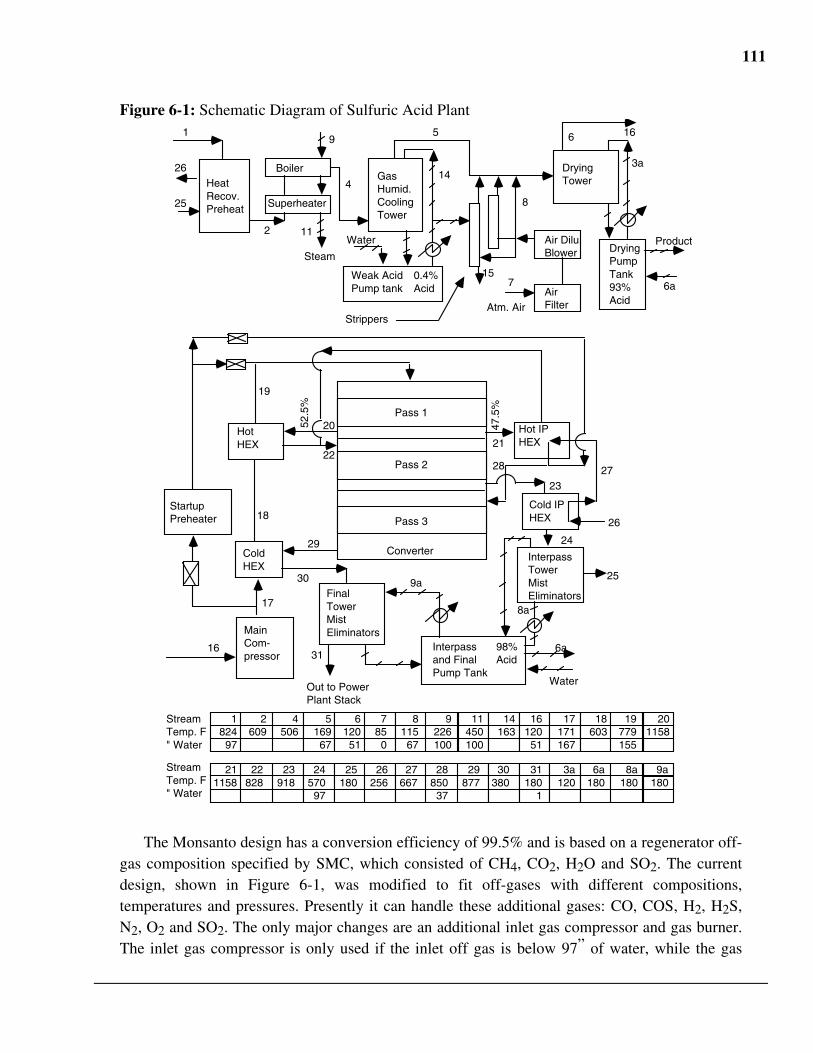
111
Figure 6-1: Schematic Diagram of Sulfuric Acid Plant
Heat Recov. Preheat
Boiler
Superheater
Gas Humid. Cooling Tower
Weak Acid Pump tank
Drying Tower
Air Filter
Air Dilu. Blower
Atm. Air
Drying Pump Tank 93% Acid
0.4% Acid
Startup Preheater
26
25
Steam
1 5
4
2
8
7
6 16
16
Pass 1
Pass 2
Pass 3
Converter
Final Tower Mist Eliminators
Interpass Tower Mist Eliminators
Hot IP HEX
Cold IP HEX
Hot HEX
Cold HEX
Interpass and Final Pump Tank
98% Acid
Main Com- pressor
17
18
19
21
20
22
2327
26
25
2429
30
31
Out to Power Plant Stack
47.5
%
52.5
%
Water
14
Strippers
9
11
15
Stream Temp. F " Water
1 824 97
2 609
4 506
5 169 67
6 120 51
7 85 0
8 115 67
9 226 100
11 450 100
14 163
16 120 51
17 171 167
18 603
19 779 155
Stream Temp. F " Water
28
3a
9a
8a
21 1158
22 828
23 918
24 570 97
25 180
26 256
27 667
28 850 37
29 877
30 380
31 180
1
3a 120
8a 180
9a 180
6a
Water
6a
Product
20 1158
6a 180
The Monsanto design has a conversion efficiency of 99.5% and is based on a regenerator off-gas composition specified by SMC, which consisted of CH4, CO2, H2O and SO2. The currentdesign, shown in Figure 6-1, was modified to fit off-gases with different compositions,temperatures and pressures. Presently it can handle these additional gases: CO, COS, H2, H2S,N2, O2 and SO2. The only major changes are an additional inlet gas compressor and gas burner.The inlet gas compressor is only used if the inlet off gas is below 97” of water, while the gas
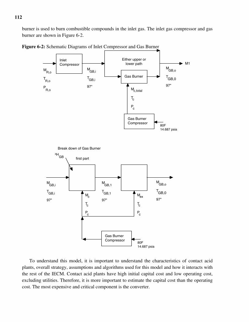
112
burner is used to burn combustible compounds in the inlet gas. The inlet gas compressor and gasburner are shown in Figure 6-2.
Figure 6-2: Schematic Diagrams of Inlet Compressor and Gas Burner
Inlet Compressor
Gas Burner
M1
M T P
R,o
R,o
R,o
M T 97"
GB,i
GB,i
Either upper or lower path
M T 97"
GB,o
GB,0
Break down of Gas Burner
first part
M T 97"
GB,i
GB,i
M T P
c,total
c
c
M T P
c
c
c
M T 97"
GB,1
GB,1
²HGB
M T P
ex
c
c
M T 97"
GB,o
GB,0
Gas Burner Compressor
80F 14.687 psia
Gas Burner Compressor
80F 14.687 psia
To understand this model, it is important to understand the characteristics of contact acidplants, overall strategy, assumptions and algorithms used for this model and how it interacts withthe rest of the IECM. Contact acid plants have high initial capital cost and low operating cost,excluding utilities. Therefore, it is more important to estimate the capital cost than the operatingcost. The most expensive and critical component is the converter.
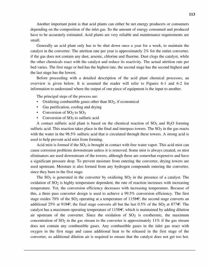
113
Another important point is that acid plants can either be net energy producers or consumersdepending on the composition of the inlet gas. So the amount of energy consumed and producedhave to be accurately estimated. Acid plants are very reliable and maintenance requirements aresmall.
Generally an acid plant only has to be shut down once a year for a week, to maintain thecatalyst in the converter. The attrition rate per year is approximately 2% for the entire converter,if the gas does not contain any dust, arsenic, chlorine and fluorine. Dust clogs the catalyst, whilethe other chemicals react with the catalyst and reduce its reactivity. The actual attrition rate perbed varies. The first stage or bed has the highest rate, the second stage has the second highest andthe last stage has the lowest.
Before proceeding with a detailed description of the acid plant chemical processes, anoverview is given below. It is assumed the reader will refer to Figures 6-1 and 6-2 forinformation to understand where the output of one piece of equipment is the input to another.
The principal steps of the process are:• Oxidizing combustible gases other than SO2, if economical• Gas purification, cooling and drying• Conversion of SO2 to SO3
• Conversion of SO3 to sulfuric acidA contact sulfuric acid plant is based on the chemical reaction of SO3 and H2O forming
sulfuric acid. This reaction takes place in the final and interpass towers. The SO3 in the gas reactswith the water in the 98.5% sulfuric acid that is circulated through these towers. A strong acid isused to help prevent acid mist from forming.
Acid mist is formed if the SO3 is brought in contact with free water vapor. This acid mist cancause corrosion problems downstream unless it is removed. Some mist is always created, so misteliminators are used downstream of the towers, although these are somewhat expensive and havea significant pressure drop. To prevent moisture from entering the converter, drying towers areused upstream. Moisture is also formed from any hydrogen compounds entering the converter,since they burn in the first stage.
The SO3 is generated in the converter by oxidizing SO2 in the presence of a catalyst. Theoxidation of SO2 is highly temperature dependent, the rate of reaction increases with increasingtemperature. Yet, the conversion efficiency decreases with increasing temperature. Because ofthis, a three pass converter design is used to achieve a 99.5% conversion efficiency. The firststage oxides 70% of the SO2 operating at a temperature of 1158•F; the second stage converts anadditional 25% at 918•F; the final stage converts all but the last 0.5% of the SO2 at 877•F. Thecatalyst has a maximum operating temperature of 1158•F, which is maintained by adding dilutionair upstream of the converter. Since the oxidation of SO2 is exothermic, the maximumconcentration of SO2 in the gas stream to the converter is approximately 11% if the gas streamdoes not contain any combustible gases. Any combustible gases in the inlet gas react withoxygen in the first stage and cause additional heat to be released in the first stage of theconverter, so additional dilution air is required to ensure that the catalyst does not get too hot.
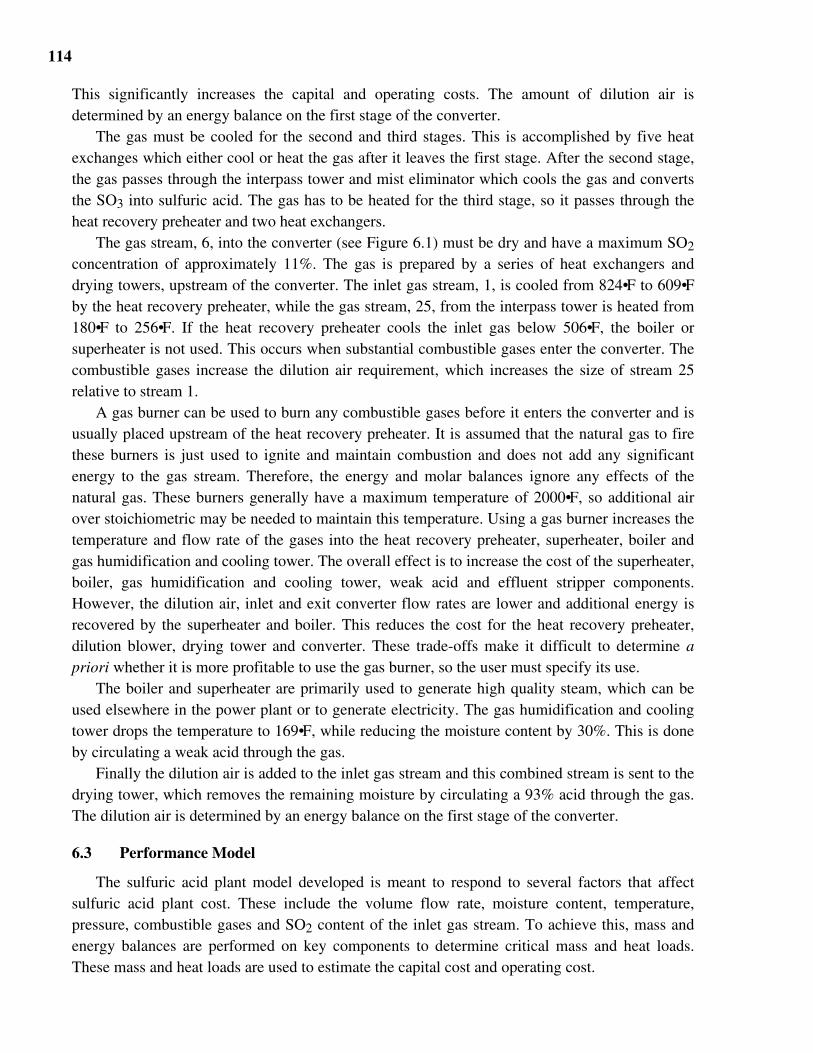
114
This significantly increases the capital and operating costs. The amount of dilution air isdetermined by an energy balance on the first stage of the converter.
The gas must be cooled for the second and third stages. This is accomplished by five heatexchanges which either cool or heat the gas after it leaves the first stage. After the second stage,the gas passes through the interpass tower and mist eliminator which cools the gas and convertsthe SO3 into sulfuric acid. The gas has to be heated for the third stage, so it passes through theheat recovery preheater and two heat exchangers.
The gas stream, 6, into the converter (see Figure 6.1) must be dry and have a maximum SO2
concentration of approximately 11%. The gas is prepared by a series of heat exchangers anddrying towers, upstream of the converter. The inlet gas stream, 1, is cooled from 824•F to 609•Fby the heat recovery preheater, while the gas stream, 25, from the interpass tower is heated from180•F to 256•F. If the heat recovery preheater cools the inlet gas below 506•F, the boiler orsuperheater is not used. This occurs when substantial combustible gases enter the converter. Thecombustible gases increase the dilution air requirement, which increases the size of stream 25relative to stream 1.
A gas burner can be used to burn any combustible gases before it enters the converter and isusually placed upstream of the heat recovery preheater. It is assumed that the natural gas to firethese burners is just used to ignite and maintain combustion and does not add any significantenergy to the gas stream. Therefore, the energy and molar balances ignore any effects of thenatural gas. These burners generally have a maximum temperature of 2000•F, so additional airover stoichiometric may be needed to maintain this temperature. Using a gas burner increases thetemperature and flow rate of the gases into the heat recovery preheater, superheater, boiler andgas humidification and cooling tower. The overall effect is to increase the cost of the superheater,boiler, gas humidification and cooling tower, weak acid and effluent stripper components.However, the dilution air, inlet and exit converter flow rates are lower and additional energy isrecovered by the superheater and boiler. This reduces the cost for the heat recovery preheater,dilution blower, drying tower and converter. These trade-offs make it difficult to determine apriori whether it is more profitable to use the gas burner, so the user must specify its use.
The boiler and superheater are primarily used to generate high quality steam, which can beused elsewhere in the power plant or to generate electricity. The gas humidification and coolingtower drops the temperature to 169•F, while reducing the moisture content by 30%. This is doneby circulating a weak acid through the gas.
Finally the dilution air is added to the inlet gas stream and this combined stream is sent to thedrying tower, which removes the remaining moisture by circulating a 93% acid through the gas.The dilution air is determined by an energy balance on the first stage of the converter.
6.3 Performance Model
The sulfuric acid plant model developed is meant to respond to several factors that affectsulfuric acid plant cost. These include the volume flow rate, moisture content, temperature,pressure, combustible gases and SO2 content of the inlet gas stream. To achieve this, mass andenergy balances are performed on key components to determine critical mass and heat loads.These mass and heat loads are used to estimate the capital cost and operating cost.
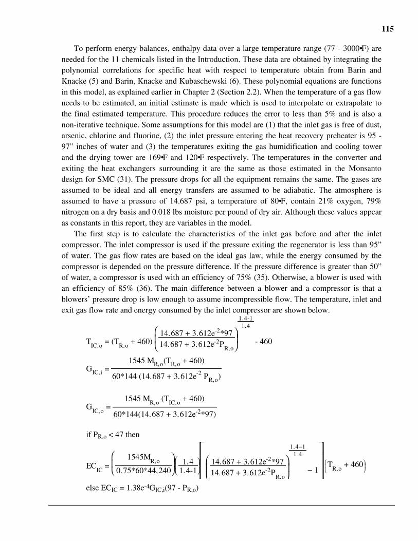
115
To perform energy balances, enthalpy data over a large temperature range (77 - 3000•F) areneeded for the 11 chemicals listed in the Introduction. These data are obtained by integrating thepolynomial correlations for specific heat with respect to temperature obtain from Barin andKnacke (5) and Barin, Knacke and Kubaschewski (6). These polynomial equations are functionsin this model, as explained earlier in Chapter 2 (Section 2.2). When the temperature of a gas flowneeds to be estimated, an initial estimate is made which is used to interpolate or extrapolate tothe final estimated temperature. This procedure reduces the error to less than 5% and is also anon-iterative technique. Some assumptions for this model are (1) that the inlet gas is free of dust,arsenic, chlorine and fluorine, (2) the inlet pressure entering the heat recovery preheater is 95 -97” inches of water and (3) the temperatures exiting the gas humidification and cooling towerand the drying tower are 169•F and 120•F respectively. The temperatures in the converter andexiting the heat exchangers surrounding it are the same as those estimated in the Monsantodesign for SMC (31). The pressure drops for all the equipment remains the same. The gases areassumed to be ideal and all energy transfers are assumed to be adiabatic. The atmosphere isassumed to have a pressure of 14.687 psi, a temperature of 80•F, contain 21% oxygen, 79%nitrogen on a dry basis and 0.018 lbs moisture per pound of dry air. Although these values appearas constants in this report, they are variables in the model.
The first step is to calculate the characteristics of the inlet gas before and after the inletcompressor. The inlet compressor is used if the pressure exiting the regenerator is less than 95”of water. The gas flow rates are based on the ideal gas law, while the energy consumed by thecompressor is depended on the pressure difference. If the pressure difference is greater than 50”of water, a compressor is used with an efficiency of 75% (35). Otherwise, a blower is used withan efficiency of 85% (36). The main difference between a blower and a compressor is that ablowers’ pressure drop is low enough to assume incompressible flow. The temperature, inlet andexit gas flow rate and energy consumed by the inlet compressor are shown below.
TIC,o
= (TR,o
+ 460) 14.687 + 3.612e-2P
R,o
14.687 + 3.612e-2*97
1.41.4-1
- 460
GIC,i = 60*144 (14.687 + 3.612e-2 PR,o)
1545 MR,o(TR,o + 460)
GIC,o
= 60*144(14.687 + 3.612e-2*97)
1545 MR,o
(TIC,o
+ 460)
if PR,o < 47 then
ECIC
= 0.75*60*44,240
1545MR,o
1.4-1
1.4
14.687 + 3.612e-2P
R,o
14.687 + 3.612e-2*97
1.41.4−1
− 1
T
R,o + 460
else ECIC = 1.38e-4GIC,i(97 - PR,o)
116
The next step is to determine if the gas burner is used and affects the gas flow rate. Themodel assumes that the pressure drop across the gas burner is negligible. The gas burner isassumed to be fired by natural gas. It is assumed that only enough natural gas is used to maintainand ignite the combustible gases in the inlet stream. Therefore, the energy and mass balancesignore the effects of it. The gas burner has a maximum operating temperature of 2000•F andcompletely oxide all the combustible gases. To prevent the gas burner from operating above2000•F, additional air is added above the stoichiometric requirement to oxides the combustiblegases. To solve for the additional air requirement, the gas burner is assumed to be divided intotwo parts, shown in Figure 6-2. The first part burns the gases with 5% excess air. If the totalenergy flow rate into the first part of the gas burner is greater than the energy flow rate of theexhaust gases at 2000•F, then additional air is added. If it isn't, then the exit temperature of thegas burner is estimated by interpolating between the inlet temperature and 2000•F. The oxygenneeded for combustion is
MO,c,1 = 2MM,R,o + 0.5MH,R,o + 0.5MCM,R,o + 1.5MCS,R,o + 1.5MHS,R,o + 2MS,R,o
The additional air needed for 5% excess air is
if 1.05MO,c,1 > MO,R,o then
MO,c = 1.05MO,c,1 - MO,R,o
else MO,c = 0
MN,c = 3.76MO,c
MW,c = 1.611*0.018(MO,c + MN,c)
Since combustion air has to be raised to 97” of water, its temperature into the gas burner is
Tc = (80 + 460) 14.68714.687 + 3.612e-2*97
1.41.4-1
- 460
The next step is to determine the exhaust gases exiting the first part of the gas burner and theenergy produced. It is assumed that all the methane, hydrogen, carbon monoxide, hydrogensulfide, sulfur and COS are oxidized.
Mj,GB,1 = 0
MSD,GB,1 = MSD,R,o + MCS,R,o + MHS,R,o + 2MS,R,o
MW,GB,1 = MW,R,o + MW,c + 2MM,R,o + MH,R,o + MHS,R,o
MCD,GB,1 = MCD,R,o + MM,R,o + MCM,R,o + MCS,R,o
MN,GB,1 = MN,R,o + MW,c
if MO,R,o > 1.05MO,c,1 then
MO,GB,1 = MO,R,o - MO,c,1
117
else MO,GB,1 = 0.05MO,c,1
where j = CM,CS,H,HS,M,S
•HGB = 345,200MM + 104,000MH + 121,700MCM + 255,400MS +
222,900MHS + 236,000MCS
Now an energy balance is performed on the first part of the gas burner to see if more air isneeded to cool the gas burner. Two estimates are made for the exit temperature: one is made atthe maximum allowable temperature of 2000•F, the other is made at the inlet temperature. If thetotal energy entering the gas burner is greater the energy flow rate of the exhaust gases at 2000•F,then additional air is needed to cool the gas. If the temperature is less than 2000•F, then noadditional air is added and the exit temperature is estimated by a linear interpolation between theinlet temperature and 2000•F. Finally, the total molar and volumetric flow rates of thecombustion air are calculated, with the energy consumed by the gas burner combustion aircompressor.
EGB,i
= ∑k=1
11 ∧h
k(T
GB,i)M
GB,i
Ec = ∧h
O(Tc)MO,c
+ ∧h
N(Tc)MN,c
+ ∧h
W,c(Tc)Mw,c
EGB,total
= EBG,i
+ Ec + ∆HGB
EGB,max
= ∑j = 1
5 ∧h
j(2000)M
j,1
EGB,min
= ∑j=1
5 ∧h
j(T
GB,i)M
j,1
where k = CD,CM,CS,H,HS,M,N,O,S,SD,W and j = CD,N,O,SD,W
if EGB,total
> EGB,max
then
MO,ex
= 15,180 -
∧h
O(Tc) + 3.76(14,440 -
∧h
N(T
c)) + 1.611*0.018*(17,920 -
∧h
W(Tc ))
EGB,total
- EGB,max
TGB,o
= 2000
118
else MO,ex
= 0
TGB,o
= E
G- E
G i
2000 - TGB,i
(EGB,total
- EGB,min
) + TGB,i
MN,ex = 3.76MO,ex
MW,ex = 1.611*0.018*4.76MO,ex
Mc,total = MO,c + MN,c + MW,c + MO,ex + MN,ex + MW,ex
Gc,total
= 60*14.687*144
1545Mc,total
(80 + 460)
ECGBC = 0.75*60*44,240
1545Mc,total
1.4-1
1.4
14.68714.687+3.612e-2*97
1.41.4-1
- 1
(80 + 460)
The next step is to determine the composition and temperature of the gas steam entering theheat recovery preheater. It should be noted that the composition of the gas stream between thegas burner and the first stage of the converter is the same, except the moisture content. Thisallows the use of the same variable names for the composition of the gas stream between the gasburner and converter, which saves space and increases execution speed. The composition of thegas stream entering the heat recovery preheater depends on whether the gas burner is used. If itisn't used, the composition and temperature are the same as those exiting the regenerator.
If a gas burner is not used then
Mk,HP,i = Mk,R,o
THP,i = TR,o
else
Mj,HP,i = 0
MSD,HP,i = MSD,GB,1
MCD,HP,i = MCD,GB,1
MW,HP,i = MW,GB,1 + MW,ex
MN,HP,i = MN,GB,1 + MN,ex
MO,HP,i = MO,GB,1 + MO,ex
THP,i = TGB,o
MHP,i
= ∑k=1
11M
k,HP,i

119
GHP,i
= 60*144*(14.687 + 3.612e-2*97)
1545MHP,i
(THP,i
+ 460)
where k = CD,CM,CS,H,HS,M,N,O,S,SD,W and j = CM,CS,H,HS,M,SSo far the algorithms have followed the gas stream into the acid plant and it seems logical to
model the heat recovery preheater next. However, the heat load on the preheater is determined bythe gas flow exiting the second stage of the converter, M25, which hasn't been determined andthis gas flow is depended on the gas flow entering the converter. This cyclic problem iseliminated by the assumptions made at the beginning of this section and noting that thecomposition of the gas entering the converter can be predicted by the composition exiting the gasburner. Another important assumption is dividing the first stage of the converter into two parts.The first part burns the combustible gases and converts 70% of the SO2 to SO3. The second partadds dilution air to lower the temperature to 1158•F. This is the same procedure used for the gasburner. Another important points are:
• The combustible gases entering the converter are the same as those exiting the gas burner.Therefore, the energy released in the first stage of the converter can be determined.
• The oxygen requirement for complete conversion of SO2 to SO3 and the oxidation of theother combustible gases can be calculated.
• The gas entering the first stage of the converter is assumed to be 997•F and free ofmoisture, since the drying tower removes all moisture.
The oxygen consumed in the first stage is calculated, with the oxygen needed for oxidationall the combustible gases and converting all the SO2 to SO3 is calculated below. This ensuresthat enough oxygen is available to convert the SO2 to SO3. Once these values are known thecomposition of the gas exiting the converter, not including additional dilution air needed tomaintain 1158•F, can be determined:
MO,CS,1 = 2MM,PH,i + 0.5MCM,PH,i + 0.5MH,PH,i + 0.35MSD,PH,i + 1.85MCS,PH,i +
1.85MHS,PH,i + 2.7MS,PH,i
MO,CS,all = 2MM,PH,i + 0.5MCM,PH,i + 0.5MH,PH,i + 0.5MSD,PH,i + 2MCS,PH,i +
2MHS,PH,i + 3MS,PH,i
if MO,CS,all > MO,PH,i then MO,CS,c = MO,CS,all - MO,PH,i
else MO,CS,c = 0
MN,CS,c = 3.76MO,CS,c
MW,CS,c = 1.611*0.018(MO,CS,c + MO,CS,c)
if MO,CS,all > MO,PH,i then MO,CS,1,o = MO,CS,all - MO,CS,1
else MO,CS,1,o = MO,PH,i - MO,CS,1
MN,CS,1,o = MN,PH,i + MN,CS,c
120
MCD,CS,1,o = MCD,PH,i + MM,PH,i + MCM,PH,i + MCS,PH,i
MW,CS,1,o = MH,PH,i + 2MM,PH,i + MHS,PH,i
MST,CS,1,o = 0.7(MSD,PH,i + 2MS,PH,i + MHS,PH,i + MCS,PH,i)
MSD,CS,1,o = 0.3(MSD,PH,i + 2MS,PH,i + MHS,PH,i + MCS,PH,i)
•HCS,1 = 42,570*0.7MSD,PH,i + 345,200MM,PH,i + 104,000MH,PH,i +
121,700MCM,PH,i + 315,000MS,PH,i + 261,500MHS,PH,i + 265,800MCS,PH,i
With this information an energy balance can be performed on the second part of the firststage to determine the additional amount of dry air needed to cool the catalyst to 1158•F. Thenthe total molar flow rate of moist dilution air can be calculated. The energy flow rate into thesecond part of the first stage is the energy flow of the species entering the heat recovery preheaterat 779•F, except the moisture, plus the energy flow from the combustion air at 779•F, plus theenergy released in the first part. The energy flow out of the second part of the first stage is thesum of the product gases at 1158•F. The constants in Equation 6.69 are the enthalpies of oxygenand nitrogen at 779•F. The constant 2864.2 in Equation 3.51 is the enthalpy difference for dry airbetween 1158•F and 779•F.
ECS,1
= ∑k =1
10 ∧h
j(779)M
k ,PH,i + 5,235.7M
O,CS,c + 5,028.4M
N,CS,c + ∆H
CS,1(6.1)
ECS,1,max
= ∑j=1
6 ∧h
j(1158)M
j,CS,1,o
Mair,CS,ex = 2,864.2
ECS,1 - ECS,1,max (6.2)
MBF = (1 + 1.611*0.018)Mair,CS,ex + MO,CS,c + MN,CS,c+ MW,CS,c
where k = CD,CM,CS,H,HS,M,N,O,S,SD and j = CD,N,O,SD,ST,W
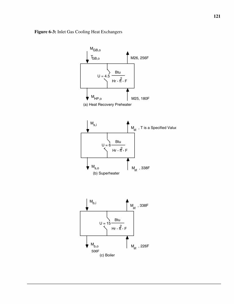
121
Figure 6-3: Inlet Gas Cooling Heat Exchangers
Btu
Hr - ft - F2
M25, 180F
M26, 256F
MGB,o
MHP,o
(b) Superheater
(a) Heat Recovery Preheater
Btu
Hr - ft - F2
M , 338F
M , T is a Specified ValueMs,i
Ms,o st
st
TGB,o
(c) Boiler
Btu
Hr - ft - F2
M , 226F
M , 338FMb,i
Mb,o st
st
506F
U = 4.5
U = 6
U = 15
122
Now the molar flow rates for the gas streams entering and exiting the drying tower and gasstreams, 23 & 25 can be determined. The gas stream entering the drying tower is the same as thegas stream entering the heat recovery preheater minus the moisture removed in the gashumidification and cooling tower plus the moist dilution air. This includes all the moisture addedwith the dilution air, since the dilution air compressor is upstream of the drying tower. The gasstreams, 23 & 25, are a bit more complicated to figure out. Stream 23 is after the second stage ofthe converter, which converts an additional 83% of the SO2 exiting the first stage to SO3, whichconsumes oxygen. Therefore, gas stream 23 is the sum of Mk,CS,1,o, the air added for temperaturecontrol, Mair,CS,ex, minus the oxygen consumed in the second stage. After the second stage itpasses through the interpass tower, which removes all the moisture and converts all the SO3 tosulfuric acid. Note that the variables MN,CS,1,o, MO,CS,1,o and MCD,CS,1,o do not include the dryair needed to cool the catalyst to 1158•F.
MD,i = MPH,i + MBF - 0.3MW,PH,i
MD,o = MD,i - 0.7MW,PH,i - 1.611*0.018Mair,CS,ex - MW,CS,c
M23
= ∑k=1
6M
k,CS,1,o + M
air,CS,ex - 0.5*0.83M
SD,CS,1,o
MCD,25 = MCD,CS,1,o
MN,25 = MN,CS,1,o+ 0.79Mair,CS,ex
MO,25 = MO,CS,1,o+ 0.21Mair,CS,ex- 0.5*0.83*MSD,CS,1,o
MSD,25 = 0.17MSD,CS,1,o
M25
= ∑j=1
4M
j,25
where k = CD,N,O,SD,ST,W and j = CD,N,O,SDWith this information, it is possible to model the heat recovery preheater, superheater and
boiler. Schematic diagrams for the heat recovery preheater, boiler and superheater are shown inFigure 6-3. The factor which will most directly affect the cost of heat exchangers are the requiredheat transfer surface area. This is calculated based on knowledge of the heat transfer load, theheat transfer coefficient U and the log mean temperature difference (LMTD) for the heatexchanger. The heat transfer coefficients for the heat recovery preheater, superheater and boilerare 4.5, 6 and 15 respectively, which are taken from the Monsanto design.
The heat load in the heat recovery preheater is energy needed to raise the gas stream, 25,from 180•F to 256•F. The exit temperature of the heat recovery preheater is estimated by makinga guess of the exit temperature based on the ratio of the heat load to the energy entering heatrecovery preheater. This algorithm is used instead of a constant since it provides a reasonableestimate of the exit temperature. This temperature estimate is used to estimate the energy flowrate exiting the heat recovery preheater. The energy estimate is used to calculate the exit
123
temperature. The exit temperature is used to calculate the log mean temperature difference,which is used to determine the area of the heat recovery preheater.
QHP
=∑j=1
4(∧h
j(256) -
∧h
j(180))M
j,25
EHP,i = ∑k=1
11 ∧hk(THP,i)Mk
Tguess = THP,i
1 -
EHP,i
QHP
Eguess = ∑k=1
11 ∧h
k(Tguess)Mk
where j = CD,N,O,SD and k = CD,CM,CS,H,HS,M,N,O,S,SD,W
THP,o
= -QHP
E
HP,i - Eguess
THP,i
- Tguess + T
HP,i
LMTDHP
=
ln T
HP o - 180
THP,i
- 256
(THP,i
- 256) - (THP,o
- 180)
AHP
= 4.5LMTD
HP
QHP
The calculations for the boiler and superheater are similar, except that first the amount ofwater that can be heated to steam must be determined and then the calculations for the LMTDand heat transfer areas of the boiler and superheater can be made. To parallel the design workperformed by Monsanto, the off-gas temperature leaving the boiler is specified as 506•F, unlessthe exit temperature of the heat recovery preheater is less. If this occurs, the superheater andboiler are not used, no steam is generated and the temperature of the gas entering the gashumidification and cooling tower is the exit temperature of the heat recovery preheater.17
The water mass flow rate required for conversion to steam is calculated by determining howmuch energy is available in the hot regenerator off-gas to heat water from 226•F to superheatedsteam at a specified temperature and 100 psia. The constant 17,929 is the energy needed to raisea mole of saturated water at 226 to 338•F, while 2134.8 is the enthalpy of saturated steam at
17 Instead of testing the exit temperature of the heat recovery preheater to see if it is greater than 506, the energy
flow of the gas stream exiting the heat recovery preheater is compared against the energy flow of the gas streamat 506. This method is used since the exit temperature is just an interpolated estimate, while the energy flowexiting the preheater can be determine more accurately by subtracting the heat load from the energy enteringthe preheater.
124
338•F. The temperature of the superheated steam is a user specified value, since this steam can beused by some FGD processes, which require steam at different temperatures.
EHP,o = EHP,i - QHP
E506 = ∑k=1
11 ∧hk(506)Mk
if EHP,o > E506 then
EGC,i = E506
TGC,i = 506
else
EGC,i = EHP,o
TGC,i = THP,o
Mst = ∧hW(Tspecified) - 2134.8 + 17,929
EHP,o - EGC,i
Now the boiler and superheater energy loads can be determined and after an energy balancecalculation, the boiler inlet temperature can be determined. The inlet temperature of the boilercan be estimated similarly to the exit temperature of the heat recovery preheater. From this, theLMTD for both the superheater and the boiler can be calculated. Finally, the required heattransfer areas for both heat exchangers are calculated from knowledge of the heat transfercoefficient, heat load and LMTD.
Qb = 17,929Mst
Qs = (∧h
W(T
specified) - 2134.8)Mst
Tguess = THP,i
1 -
EHP,i
QHP
Eguess = ∑k=1
11 ∧h
k(Tguess)Mk
Tbi,i
= -Qs EHP,o
- Eguess
THP,o
- Tguess + T
HP,o
The log mean temperature differences for the boiler and superheater are based on the inletand outlet temperatures of the two heat exchangers. The required heat transfer surface area for
125
each is calculated based on the heat load, the log mean temperature difference and the universalheat transfer coefficient. The values for the heat transfer coefficients are adopted from theMonsanto estimate.
LMTDs =
ln T
b i - 338
THP,o
- Tspecified
(THP,o
- Tspecified
) - (Tb,i
- 338)
LMTDb =
ln 506 - 226
Tb,i
- 338
(Tb,i
- 338) - (506 - 226)
As = 6LMTDs
Qs
Ab =
15LMTDb
Qb
The off-gas enters the cooling and humidification tower at a temperature of 506•F and leavesat 169•F. It is assumed that about 30 percent of the water vapor is removed based on theMonsanto design. Cooling is effected by the circulation of a weak acid stream through thecooling tower. The mass flow of this stream is calculated by an energy balance. The constant324.6 is amount of energy needed to raise the temperature of the weak acid from 163•F to 181•F.The constants 840.6 and 17,813 are the enthalpy and heat of vaporization at 181•F.
EGC,o = ∑k=1
11 ∧hk(169)Mk - 0.3
∧hW(169)MW,HP,i
MWA
= 324.6
EGC,i
- EGC,o
+ 0.3(∧h
W(T
GC,i) - 840.6 + 17,813
The electricity usage for the main and dilution compressors and also the pumps used for thestrong, weak and product acid pumps can be determined. The pressure drops across the main anddilution compressors are 116” and 67” of water respectively.
ECBF
= 0.75*60*44240
1545MBF
1.4-1
1.4
14.68714.687 + 3.612e-2*67
1.41.4-1
- 1
(80 + 460)
ECMC =
0.75*60*44240
1545MD,o
1.4-1
1.4
14.687 + 3.612e-2*51
14.687 + 3.612e-2*167
1.41.4-1
- 1
(120 + 460)
The total acid produced can be determined with the energy consumption of the pumps. Thepressure drops for the strong, weak and product acid pumps are 80 feet of water, 120 psi and 80psi respectively. The efficiencies for the strong and weak acid pumps are 80%, while the product
126
pump is much smaller and has an efficiency of 70%. The specific gravity for sulfuric acid greaterthan 95% is 1.83, while the specific gravity for weak acid is assumed to be 1. The specificgravity for the product acid at 93% concentration, is estimated to be 1.77, which equals 1.83*.93+ 1*0.07. The energy needed for the weak acid pump is based on the molar flow rate of weakacid. The strong acid system which supplies acid to the drying, interpass and final towers hasthree pumps. Therefore, the energy usage is based on scaling the total flow rate for these pumpson the sulfuric acid produced. In the Monsanto design, 3501 gallons per minute of strong acid ispumped against a head of 80 feet of water for 17.3 tons per hour of acid produced.
macid = 0.995 (MSD,R,o + MCS,R,o + MHS,R,o + 2MS,R,o) * 98 lbm/lb•mole
/ 2000 tons/lbm
ECWA
= 44,240
kWft-lbf/min*7.4805
ft3gal
*60hr
min*8.33gallbm*0.80
120in2lbf *18
lbmolelbm *144
ft2in2
MWA
which simplifies to
ECWA
= 63,813
kWlbmole/hr * lbf/in2
*0.80
120in2lbf M
WA
ECSS
= 7.4805
ft3gal
*32.174lbf-sec2lbm-ft *44,240
kWft-lbf/min*0.80
17.3
hrtons
3501mingal
80 ft * 61.2ft3lbm*32.174
sec2ft *1.83m
acid
which simplifies to
ECSS = 2955
kWgal/min*ft
*0.80
202.4tons/hrgal/min
*80 ft macid
ECPA
= 60
hrmin*8.33
gallbm*7.4805
ft3gal
*44,240kW
ft-lbf/min*1.77*0.70
2000tonlbm*144
ft2in2
*80in2lbf m
acid
which simplifies to
ECPA = 1017
kWtons/hr lbf/in2
*0.70
80in2lbf macid
The total energy consumed is the sum of the inlet, gas burner, dilution air and maincompressor plus the weak, strong and product acid pumps. The equivalent electric power of the
127
steam produced is calculated by assuming an 88% efficient boiler and the heat rate specified bythe main power plant.
ECtotal = ECIC + ECGB + ECBF + ECMC + ECWA + ECSS + ECPA
ECst = 0.88HR
EPH,o
- EGC,i
6.4 Economic Model
The cost estimate for the sulfuric acid plant is based on physical parameters that affect thecost of the equipment in the plant. An experimental scaling factor of 0.6 is assumed and all thecapital costs are in mid-83 dollars, except the inlet compressor and gas burner which are mid-82dollars. All costs may later be adjusted to a current basis using appropriate cost-escalatorsincluded in the IEC model.
6.4.1 Capital CostThe cost of the inlet compressor depends on the pressure drop and the inlet gas flow rate. The
cost is pro-rated by pressure drop since the capital cost of blowers and compressors increase withincreasing pressure. The cost estimates come from the NOXSO chapter in the EPRI EconomicEvaluation of FGD Systems (22). For both estimates, it is assumed that there are two operatingand one spare. The algorithm is:
if PR,o < 47” of water
DCCIC
= $1.04e6 35,000ft3/min
GR,o
0.6
314
Cidx
else if 47 <= PR,o < 95
DCCIC = $5.64e6 1.80e6 ft
3/min
GR,o
0.6
314
Cidx
The capital gas of the gas burner is also taken from reference (22). It is assumed that there aretwo operating and one spare and that the cost includes the cost of the combustion air compressor.
DCCGB
= $7.07e5 68,000 ft3/min
GIC,o
0.6
314
Cidx
The heat recovery preheater cost is scaled to the Monsanto cost estimate of $29,000 for a heatexchanger with an area of 1100 square feet. The cost of the boiler is based on an estimated costof $53,000 for a heat exchanger with 350 square feet of heat exchange area. The cost of thesuperheater is scaled from the estimate of $80,000 for a heat exchanger with an area of 50 squarefeet.
128
DCCHP = $29,000 1,100ft
2
AHP
0.6
316.9
Cidx
DCCb = $53,000
350ft2
Ab
0.6
316.9
Cidx
DCCs = $80,000 50ft2
As
0.6
316.9
Cidx
The gas humidification and cooling tower cost estimate is based on the Monsanto estimate of$367,000 for a gas stream of 1063 lb•mole/hr. The cost of the tower is scaled to the off-gas flowMGC,i entering the sulfuric acid plant.
DCCGC
= $367,000 1,063 lbmole/hr
MGC
0.6
316.9
Cidx
The weak acid system is associated with the gas humidification and cooling tower. The costof this system is proportional to the flow rate of weak acid, MWA, required to achieve thenecessary cooling in the tower.
DCCWA
= $39,000 19,250 lbmole/hr
MWA
0.6
316.9
Cidx
The drying tower is sized to accommodate the inlet gas stream consisting of the regeneratoroff-gas and dilution air, MD,i. Monsanto estimated a cost of $636,000 for a tower that handles5325 lb•mole/hr of gas.
DCCD = $636,000
5,325 lbmole/hr
MD,i
0.6
316.9
Cidx
The blower and filter are required to pump and clean the dilution air mass flow, MBF and aresized accordingly. Monsanto estimated the cost of these components based on a dilution air inletflow of 4407 lb•mole/hr.
DCCBF
= $518,000 4,407 lbmole/hr
MBF
0.6
316.9
Cidx
The contact section of the sulfuric acid plant includes the inter-pass heat exchangers and thecatalytic converter. The total cost of this part of the system was estimated by Monsanto to be$2,681,000. The cost of this part of the plant is scaled to the gas flow exiting the drying tower.
DCCCS
= $2,681,000 4,854 lbmole/hr
MD,o
0.6
316.9
Cidx
129
The cost for the interpass and final towers and their associated equipment was estimated to be$988,000. This cost is scaled to the gas stream M23.
DCCT = $988,000 4,685 lbmole/hr
M23
0.6
316.9
Cidx
The strong acid system is proportional in size to the amount of sulfur in the off-gas stream.The cost of the effluent stripper is assumed to be proportional to the off-gas flow rate.
DCCSA
= $739,000 354 lbmole/hr
MSD,HP,i
+ MCS,HP,i
+ MHS,HP,i
+ 2MS,HP,i
0.6
316.9
Cidx
DCCES
= $70,000 1,063 lbmole/hr
MGC,i
0.6
316.9
Cidx
The total direct cost of the sulfuric acid plant is the sum of the individual equipment directcapital costs. The indirect capital cost, not including AFUDC, is estimated to be 27.5%, 41.9%and 8.1% of the total direct cost for the labor and general field cost, home office cost andcontingency respectively.
DCCtotal
= ∑k=1
13DCC
k
TCCacid = (1 + 0.275 + 0.419 + 0.081)DCCtotal= 1.776DCCtotal
6.4.2 Operating and Maintenance CostsThe non-utility operating costs of an acid plant consist of the operating, maintenance and
administration labor, plus maintenance material, catalyst makeup, marketing and shipping cost.The labor costs and makeup requirements are estimated from letters with Monsanto (33, 34). Themaintenance personnel are assumed to only work 1/3 of the total number of hours in a year. It isassumed that 2 operators are always working around the clock. Acid plants of this size require 2operators per shift, with 2 full time maintenance people. The administration and support laborcost is estimated to be 30% of the operating and maintenance labor cost.
OCoper = 2 persons * 19.70 $/hr * 8766 hrs/yr * Cidx/325.3
OCmaint-labor = 2 persons * 19.70 $/hr * 8766 hrs/yr / 3 * Cidx/325.3
OCadmin = 0.30 * (OCoper + OCmaint-labor)
The maintenance material cost is estimated as a fraction of the direct capital cost. Thefraction is 0.9%. The makeup of the catalyst is approximately 2% per year and the converterrequires approximately $35.2 per lb•mole/hr of gas flow (1985$) (34). The marketing andshipping cost are estimated to be 10% of the sulfuric acid credit (12). Sulfuric acid is assumed tosell for $50/ton (1985$). (12).
OCmaint-matl = 0.009 * DCCtotal
130
OCmakeup = 0.02 * 35.2 85$/lb•mole/hr * M6 * Cidx/325.3
OCcredit = 50 85$/ton * CF * 8766 * macid * Cidx/325.3
OCmarketing = 0.1 * OCcredit
OCtotal = OCoper + OCmaint-labor + OCadmin + OCmain-mater + OCmakeup
+ OCmarketing - OCcredit
6.5 Numerical Example
This section contains a numerical example of the sulfuric acid plant model presented in theprevious sections. The input parameters and their values necessary to run the model are given inTable 6-1. The model will be illustrated by using a gas stream with a large quantity ofcombustible gases, which requires the use of the gas burner. The gas stream is not from anyparticular report or FGD process. The composition consists of the species with which this modelhas been designed for except nitrogen and oxygen.18 The pressure exiting the regenerator in theFGD process is 28” of water. Therefore, the inlet compressor is required to raise the pressure to97” of water.
Since the pressure of the regenerator off-gas is less than 97” of water, the inlet compressor isneeded. Equations 6.3, 6.4, 6.5 and 6.6 are used to calculate the temperature exiting the inletcompressor, gas flow rate in actual cubic feet per minute and electricity consumption of thecompressor.
TIC,o
= (TR,o
+ 460) 14.687 + 3.612e-2P
R,o
14.687 + 3.612e-2*97
1.41.4-1
- 460(6.3)
TIC,i = (550 + 460) 14.687 + 3.612e-2*28
14.687 + 3.612d-2
*97
1.41.4-1
- 460
TIC,i = 958.5•F
GIC,i
= 60*144 (14.687 + 3.612e-2 P
R,o)
1545 MR,o
(TR,o
+ 460)(6.4)
GIC,i
= 60*144(14.687 + 3.612e-2*28)
1545*1,568*(550 + 460)
GIC,i = 24,290 acfm
18 There are two reasons for not including oxygen and nitrogen in the gas stream for the numerical example.
Since there are products of incomplete oxidation in this particular gas stream, it is not likely to contain oxygen.Nitrogen could have been added to the gas; however, any nitrogen available would probably have been addedwith air to completely oxidize the gas in the regenerator.
131
GIC,o
= 60*144(14.687 + 3.612e-2*97)
1545 MR,o
(TIC,o
+ 460)(6.5)
Table 6-1: Input Parameters for Sulfuric Acid Plant Numerical Example
Input Parameter Sample Value Input Parameter Sample Value
TR,o 900•F MM,R,o 10 lb•mole/hrPR,o 28” of water MN,R,o 0 lb•mole/hrTspecified 550•F MO,R,o 0 lb•mole/hrMCD,R,o 500 lb•mole/hr MS,R,o 41 lb•mole/hrMCO,R,o 50 lb•mole/hr MSD,R,o 200 lb•mole/hrMCOS,R,o 17 lb•mole/hr MW,R,o 500 lb•mole/hrMH,R,o 100 lb•mole/hr MR,o 1,568 lb•mole/hrMHS,R,o 150 lb•mole/hr
GIC,o
= 60*144*(14.687 + 3.612e-2*97)
1,545*1,568*(958.54 + 460)
GIC,o = 21,865 acfm
if PR,o < 47 then
ECIC
= 0.75*60*44,240
1545MR,o
1.4-1
1.4
14.687 + 3.612e-2P
R,o
14.687 + 3.612e-2*97
1.41.4-1
- 1
T
R,o
+ 460 (6.6)
else ECIC = 1.38e-4GIC,i(97 - PR,o)
Since 28” is less than 97”
ECIC
= 0.75*60*44,240
1,545*1,568
1.4-1
1.4
14.687 + 3.612e-2*28
14.687 + 3.612e-2*97
1.41.4-1
- 1
(TR,o
+ 460)
ECIC = 249.3 kW
The gas burner is used since the inlet gas contains many combustible gases. The algorithm ofthe gas burner divides it into two parts, see Figure 6-3. The first part determines the amount ofenergy released by burning the combustible gases. This is used to determine the total energy flowexiting the first part of the gas burner and the composition of the outlet gas. The air needed forcombustion and its temperature are calculated first.
132
MO,c,1 = 2MM,R,o + 0.5MH,R,o + 0.5MCM,R,o + 1.5MCS,R,o + 1.5MHS,R,o + 2MS,R,o
MO,c,1 = 2*10 + 0.5*100 + 0.5*50 + 1.5*17 + 1.5*150 + 2*41 = 427.5 lb•mole/hr
since 1.05*427.5 > 0
MO,c = 1.05*427.5 - 0 = 448.9 lb•mole/hr
MN,c = 3.76MO,c = 3.76*448.88 = 1,688 lb•mole/hr
MW,c = 1.611*0.018(448.88 + 1,687.77) = 61.96 lb•mole/hr
Tc = (80 + 460) 14.68714.687 + 3.612e-2*97
1.41.4-1
- 460
Tc = 114.1•F
Now the exhaust gas from the first part and the energy released are calculated.
MCO,GB,1 = MCOS,GB,1 = MH,GB,1 = MHS,GB,1 = MM,GB,1 = MS,GB,1 = 0
MSD,GB,1 = MSD,R,o + MCS,R,o + MHS,R,o + 2MS,R,o
MSD,GB,1 = 200 + 17 + 150 + 2*41 = 449 lb•mole/hr
MW,GB,1 = MW,R,o + MW,c + 2MM,R,o + MH,R,o + MHS,R,o
MW,GB,1 = 500 + 61.96 + 2*10 + 100 + 150 = 832.0 lb•mole/hr
MCD,GB,1 = MCD,R,o + MM,R,o + MCM,R,o + MCS,R,o
MCD,GB,1 = 500 + 10 + 50 + 17 = 577 lb•mole/hr
MN,GB,1 = MN,R,o + MW,c
MN,GB,1 = 0 + 1,688 = 1,688 lb•mole/hr
since 0 > 1.05*427.5 is false
MO,GB,1 = 0.05MO,c,1 = 0.05*417.5 = 21.38
•HGB = 345,200MM + 104,000MH + 121,700MCM + 255,400MS +
222,900MHS + 236,000MCS
•HGB = 345,200*10 + 104,000*100 + 121,700*50 + 255,400*41+
222,900*150 + 236,000*17
•HGB = 67.86e6 Btu/hr
The total energy exiting the first part of the gas burner is calculated next, with the energyflow rates of the exhaust gases at two estimated temperatures 2000•F and 958.54•F. Then theenergy flow exiting the first part is compared to the energy flow rate of the exhaust gas, if it isgreater than additional air is needed to cool the gas burner. Then the total volumetric flow rate of
133
the combustion gas is calculated with the electricity consumed by the compressor for thecombustion air.
EGB,i
= ∑k=1
11 ∧h
k(T
GB,i)M
GB,i = ∑
k=1
11 ∧h
k(958.54)M
GB,i
EGB,i = 9,567*500 + 6,414*50 + 10.34e3*17 + 6,166*100 +7,950*150 +
10,33e3*10 + 6,359*0 + 7.426*41 + 9,833*200 + 7,576*500
EGB,i = 13.25e6 Btu/hr
Ec = ∧h
O(Tc)MO,c
+ ∧h
N(Tc)MN,c
+ ∧h
W,c(Tc)Mw,c
Ec = 261.3*448.9 + 258.6*1,688 + 298.2*61.96 = 572.2e3 Btu/kr
EGB,total
= EBG,i
+ Ec + ∆HGB
EGB,total = 13.25e6 + 572.2e3 + 67.86e6 = 81.68e6
EGB,max
= ∑j = 1
5 ∧h
j(2000)M
j,1
EGB,max = 22.78e3*577 + 14.44e3*1,688 + 15.18e3*21.38 + 23.36e3*449 +
17.92e3*832.0
EGB,max = 63.24e6 Btu/hr
EGB,min = ∑j=1
5 ∧hj(TGB,i)Mj,1
EGB,min = 9,569*577 + 6,359*1,688 + 6,640*21.38 + 9,833*449 + 7,576*832.0
EGB,min = 27.11e6 Btu/hr
134
if EGB,total
> EGB,max
then
MO,ex
= 15,180 -
∧h
O(T
c) + 3.76(14,440 -
∧h
N(T
c)) + 1.611*0.018*(17,920 -
∧h
W(T
c))
EGB,total
- EGB,max
TGB,o
= 2000
else MO,ex
= 0
TGB,o
= E
GB,max - E
GB,min
2000 - TGB,i
(EGB,total
- EGB,min
) + TGB,i
since 81.68e6 > 63.24e6
MO,ex
= (15,180 - 261.3) + 3.76(14,440 - 258.6) + 1.611*0.018*4.76(17,920 - 298.2)
81.68e6 - 63.24e6
MO,ex = 260.9 lb•mole/hr
TGB,o = 2000•F
MN,ex = 3.76MO,ex = 3.76*260.9 = 981.1 lb•mole/hr
MW,ex = 1.611*0.018*4.76MO,ex = 1.611*0.018*4.76*260.9 = 36.02 lb•mole/hr
Mc,total = MO,c + MN,c + MW,c + MO,ex + MN,ex + MW,ex
Mc,total = 448.9 + 1,688 + 61.96 + 260.9 + 981.1 + 36.02 = 3,477 lb•mole/hr
Gc,total
= 60*14.687*144
1,545Mc,total
(80 + 460) =
60*14.687*1441,545*3,477*(80 + 460)
= 22,860 acfm
ECGB = 0.75*60*44,240
1545Mc,total
1.4-1
1.4
14.68714.687+3.612e-2*97
1.41.4-1
- 1
(80 + 460)
ECGB
= 0.75*60*44,240
1,545*3,477
1.4-1
1.4
14.68714.687 + 3.612e-2*97
1.41.4-1
- 1 (80 + 460)
ECGB =321.8 kW
Since the gas burner is used, the actual exhaust gas and volumetric gas flow rate needs to becalculated. It is important to note that the molar flow rate has tripled, while the volumetric flow
135
rate has increased almost five times. Since the gas burner is upstream of the superheater andboiler, the energy released in the gas burner can be partially recovered by the superheater andboiler.
MCO,HP,i = MCOS,HP,i = MH,HP,i = MHS,HP,i = MM,HP,i = MS,HP,i = 0 lb•mole/hr
MSD,HP,i = MSD,GB,1 = 449 lb•mole/hr
MCD,HP,i = MCD,GB,1 = 577 lb•mole/hr
MN,HP,i = MN,GB,1 + MN,ex = 1,688 + 981.1 = 2669 lb•mole/hr
MO,HP,i = MO,GB,1 + MO,ex = 21.38 + 260.9 = 282.3 lb•mole/hr
MW,HP,i = MW,GB,1 + MW,ex = 832.0 + 36.02 = 868.0 lb•mole/hr
THP,i = TGB,o = 2000•F
MHP,i
= ∑k=1
11M
k,HP,i = 577 + 2,669 + 282.3 + + 449 + 868.0 = 4,845 lbmole/hr
GHP,i
= 60*144*(14.687 + 3.612e-2*97)
1,545MHP,i
(THP,i + 460)
= 60*144*(14.687 + 3.612e-2*97)
1,545*4,845*(2,000 + 460)
GHP,i = 117.2e3 acfm
The next step is to calculate the oxygen needed for the converter and the energy released inthe first stage of the converter. The first stage of the catalytic converter is divided into two partsto solve for dilution air. The first part burns any combustibles and converts above 70% of theSO2 to SO3.
MO,CS,1 = 2MM,PH,i + 0.5MCM,PH,i + 0.5MH,PH,i + 0.35MSD,PH,i + 1.85MCS,PH,i +
1.85MHS,PH,i + 2.7MS,PH,i lb•mole/hr
MO,CS,1 = 2*0 + 0.5*0 + 0.5*0 + 0.35*449 + 1.85*0 + 1.85*0 + 2.7*0 = 157.2
MO,CS,all = 2MM,PH,i + 0.5MCM,PH,i + 0.5MH,PH,i + 0.5MSD,PH,i + 2MCS,PH,i +
2MHS,PH,i + 3MS,PH,i
MO,CS,all = 20 + 0.5*0 + 0.5*0 + 0.5*449 + 2*0 + 2*0 + 3*0 = 224.5 lb•mole/hr
if MO,CS,all > MO,PH,i then MO,CS,c = MO,CS,all - MO,PH,i
else MO,CS,c = 0
since 224.5 is not greater than 282.3 then
MO,CS,c = 0 lb•mole/hr
MN,CS,c = 3.76MO,CS,c = 3.76*0 = 0 lb•mole/hr
136
MW,CS,c = 1.611*0.018(MO,CS,c + MO,CS,c) = 1.611*0.018(0 + 0) = 0 lb•mole/hr
if MO,CS,all > MO,PH,i then MO,CS,1,o = MO,CS,all - MO,CS,1
else MO,CS,1,o = MO,PH,i - MO,CS,1
since 224.5 is not greater than 282.3 then
MO,CS,1,o = MO,PH,i - MO,CS,1 = 282.3 - 157.2 = 125.2 lb•mole/hr
MN,CS,1,o = MN,PH,i + MN,CS,c = 2,669 + 0 = 2,669 lb•mole/hr
MCD,CS,1,o = MCD,PH,i + MM,PH,i + MCM,PH,i + MCS,PH,i
MCD,CS,1,o = 577 + 0 + 0 + 0 + 0 = 577 lb•mole/hr
MW,CS,1,o = MH,PH,i + 2MM,PH,i + MHS,PH,i = 0 + 0 + 2*0 = 0 lb•mole/hr
MST,CS,1,o = 0.7(MSD,PH,i + 2MS,PH,i + MHS,PH,i + MCS,PH,i)
MST,CS,1,o = 0.7(449 + 0 + 0 + 0 + 0) = 314.3
MSD,CS,1,o = 0.3(MSD,PH,i + 2MS,PH,i + MHS,PH,i + MCS,PH,i)
MSD,CS,1,o = 0.3(449 + 0 + 0 + 0 + 0) = 134.7
•HCS,1 = 42,570*0.7MSD,PH,i + 345,200MM,PH,i + 104,000MH,PH,i +
121,700MCM,PH,i + 315,000MS,PH,i + 261,500MHS,PH,i + 265,800MCS,PH,i
•HCS,1 = 42,570*0.7*449 + 345,200*0+ 104,000*0 + 121,700*0 + 315,000*0
+ 261,500*0+ 265,800*0 = 13.38e6
An energy balance can be made to determine the amount of air needed for cooling the firststage of the converter. Once this value is known, the total amount of moist dilution air can bedetermined with the molar flow rates exiting the drying tower (M6), second stage (M23) andentering the heat recovery preheater (M25).
ECS,1
= ∑k =1
10 ∧h
j(779)M
k ,PH,i + 5,235.7M
O,CS,c + 5,028.4M
N,CS,c + ∆H
CS,1
ECS,1= 7,456*577 + 5,068*0 + 8,082*0 + 4,888*0 + 6,202*0 + 7,779*0 +
5,028*2,669 + 5,236*282.3 + 5,869*0 + 7,680*449 + 5,236*0 + 5,028*0 +
13.38e6
ECS,1 = 36.03e6 Btu/hr
ECS,1,max
= ∑j=1
6 ∧h
j(1158)M
j,CS,1,o
137
ECS,max= 11,980*577 + 7,859*2,669 + 8,226*125.2 + 12,290*134.7 + 16,970*314.3
+9,439*0
ECS,max= 35.91e6 Btu/hr
where k = CD,CM,CS,H,HS,M,N,O,S,SD and j = CD,N,O,SD,ST,W
Mair,CS,ex = 2,864.2
ECS,1 - ECS,1,max =
2,864.236.03e6 - 35.91e6
= 42.53 lbmole/hr
MBF = (1 + 1.611*0.018)Mair,CS,ex + MO,CS,c + MN,CS,c + MW,CS,c
MBF = (1 + 1.611*0.018)42.53 + 0 + 0 + 0 = 43.76 lb•mole/hr
MD,i = MPH,i + MBF - 0.3MW,PH,i = 4845 + 43.76 - 0.3*868.0 = 4,629 lb•mole/hr
MD,o = MD,i - 0.7MW,PH,i - 1.611*0.018Mair,CS,ex - MW,CS,c
MD,o = 4,629 - 0.7*868.0 - 1.611*0.018*43.76 - 0 = 4,020 lb•mole/hr
M23
= ∑k=1
6M
k,CS,1,o + M
air,CS,ex - 0.5*0.83M
SD,CS,1,o
M23 = 577 + 2,669 + 125.2 + 134.7 + 314.3 + 0 + 42.53 - 0.5*0.83*134.7
M23 = 3,807 lb•mole/hr
MCD,25 = MCD,CS,1,o = 577 lb•mole/hr
MN,25 = MN,CS,1,o+ 0.79Mair,CS,ex = 2,669 + 0.79*42.53 = 2,702 lb•mole/hr
MO,25 = MO,CS,1,o+ 0.21Mair,CS,ex- 0.5*0.83*MSD,CS,1,o
MO,25 = 125.2 + 0.21*42.53 - 0.5*0.83*134.7
MO,25 = 78.19 lb•mole/hr
MSD,25 = 0.17MSD,CS,1,o = 0.17*134.7 = 22.90 lb•mole/hr
M25 = ∑j=1
4
Mj,25 = 577 + 270 + 78.18 + 22.90 = 3,381 lbmole/hr
where k = CD,N,O,SD,ST,W and j = CD,N,O,SDThe heat load on the heat recovery preheater can be determined now. The initial guess for the
exit temperature is estimated by the ratio of the heat load to the inlet energy flow rate. Thisalgorithm is used because it makes a very good initial guess for a wide range of inlettemperatures, compositions and heat loads. Note that in Equations 6.7 and 6.8, the molar flowrates of the combustible gases are zero and weren't shown in the calculation.
138
QHP
=∑j=1
4(∧h
j(256) -
∧h
j(180))M
j,25
QHP = (1,715 - 961.0)*577 + (1,256 - 720.3)*2,702 + (1,285 - 732.3)*78.19 +
(1,802 - 1,017)*22.29
QHP = 1.943e6 Btu/hr
EHP,i
= ∑k=1
11 ∧h
k(T
HP,i)M
k = ∑
k=1
11 ∧h
k(2000)M
k(6.7)
EHP,i = 22.78e3*577 + 14.44e3*2,669 + 15.18e3*282.3 + 23.36e3*449 +
17.92e3*868.0
EHP,i = 82.01e6 Btu/hr
Tguess = THP,i
1 -
EHP,i
QHP
= 2,000
1 -
82.01e61.943e6
= 1,953
oF
Eguess = ∑k=1
11 ∧hk(Tguess)Mk = ∑
k=1
11 ∧hk(1,953)Mk
(6.8)
Eguess = 22.15e3*577 + 14.06e3*2,669 + 14.78e3*282.3 +22.70e3*449 +
17.42e3*868.0
Eguess = 79.79e6 Btu/hr
where j = CD,N,O,SD and k = CD,CM,CS,H,HS,M,N,O,S,SD,W
THP,o
= -QHP
E
HP,i - Eguess
THP,i
- Tguess + T
HP,i = -1.943e6
82.01e6 - 79.79e6
2,000 - 1,953 + 2,000 = 1,959
oF (
LMTDHP
=
ln T
HP,o - 180
THP,i
- 256
(THP,i
- 256) - (THP,o
- 180) =
ln 2,000 - 1801,959 - 256
(2,000 - 256) - (1,959 - 180) = 1,761
oF
AHP = 4.5LMTDHP
QHP = 4.5*1,7611.943e6
= 245.1 ft2
The amount of steam generated with the heat and area of the boiler and superheater, aredetermined similarly to the heat recovery preheater. The energy flow rate exiting the heat
139
recovery preheater is compared to the energy flow at 506•F to determine if any steam can begenerated.
EHP,o = EHP,i - QHP = 82.01e6 - 1.943e6 = 80.07 Btu/hr
E506 = ∑k=1
11 ∧hk(506)Mk
E506 = 4,366*577 + 3,040*2,669 + 3,143*282.3 + 4,527*449 + 3,556*868.0
E506 = 16.64e6 Btu/hr
and k = CD,CM,CS,H,HS,M,N,O,S,SD,W if E
HP,o > E
506 then
EGC,i
= E506
TGC,i
= 506 e l s e
E G C , i = E H P , o
TG C , i
= TH P , o
since 80.07e6 is greater than 16.64e6
EGC,i= 16.64e6 Btu/hr
TGC,i = 506•F
Mst = ∧h
W(T
specified) - 2,134.8 + 17,929
EHP,o
- EGC,i
= 3,934 - 2,134.8 + 17,929
80.07e6 - 16.64e6
Mst = 3215 lb•mole/hr
Now the boiler and superheater heat loads and also the log mean temperature differences andareas can be determined. It should be noted that the model is not smart enough to determinewhether the exit temperature of the heat recovery preheater is lower than the specifiedtemperature of the steam. If this occurs, a warning will be generated by the model when themodel tries to evaluate the log mean temperature difference for the superheater. At this point theuser should check the exit temperature of the heat recovery preheater and set the temperature ofthe steam accordingly.
Qb = 17,929Mst = 17,929*3,215 = 57.65e6 Btu/hr
Qs = [∧hW(Tspecified) - 2134.8]Mst = (3,934 - 2,134.8)*3,215 = 5,786e6 Btu/hr
Tguess = THP,o
1 - E HP,o
Qs
= 1 , 9 5 9 1 -
80.07e65.768e6
= 1,817
oF
140
Eguess = ∑k=1
11 ∧h
k(Tguess)Mk
= ∑k=1
11 ∧h
k(1,817)M
k
Eguess = 20.35e3*577 + 12.98e3*2,669 + 13.63e3*282.3 + 20.86e3*449 +
15.99e3*868.0
Eguess = 73.49e6 Btu/hr
Tbi,i
= -Qs EHP,o
- Eguess
THP,o
- Tguess + T
HP,o = -5.786e6
80.07e6 - 73.49e6
1,959 - 1,817 + 1,959 = 1,834
oF
LMTDs =
ln T
b,i - 338
THP,o
- 338
(THP,o
- Tspecified
) - (Tb,i
- 338) =
ln 1,834 - 3381,959 - 550
(1,959 - 550) - (1,834 - 338) = 1,452
oF
LMTDb =
ln 506 - 226
Tb,i
- 338
(Tb,i
- 338) - (506 - 226) =
ln 506 - 2261,834 - 338
(1,834 - 338) - (506 - 226) = 725.8
oF
As = 6LMTDs
Qs = 6*1,4525.786e6
= 664 ft2
Ab =
15LMTDb
Qb =
15*725.857.65e6
= 5,295 ft2
The weak acid needed for the gas humidification and cooling tower and also the electricityconsumption of the compressors and pumps can be calculated now.
EGC,o
= ∑k=1
11 ∧h
k(169)M
k - 0.3
∧h
W(169)M
W,HP,i
EGC,o= 854.7*577 + 643.1*2,669 + 653.2*282.3 + 905.2*449 + 742.9*868.0 -
0.3*742.9*868.0
EGC,o = 3.252e6 Btu/hr
MWA
= 324.6
EGC,i
- EGC,o
+ 0.3(∧h
W(T
GC,i) - 840.6 + 17,813)M
W,HP,i
141
MWA = 324.6
16.64e6 - 3.252e6 + 0.3(3,556 - 840.6 + 17,813)868.0
MWA = 57,710 lb•mole/hr
ECBF
= 0.75*60*44240
1545MBF
1.4-1
1.4
14.68714.687 + 3.612e-2*67
1.41.4-1
- 1
(80 + 460)
ECBF
= 0.75*60*44,240
1,545*43.76
1.4-1
1.4
14.68714.687 + 3.612e-2*67
1.41.4-1
- 1 (80 + 460)
ECBF = 2.862 kW
ECMC =
0.75*60*44240
1545MD,o
1.4-1
1.4
14.687 + 3.612e-2*51
14.687 + 3.612e-2*167
1.41.4-1
- 1
(120 + 460) (
ECMC
= 0.75*60*44,240
1,545*4,020
1.4-1
1.4
14.687 + 3.612e-2 *5114.687 + 3.612e-2*167
1.41.4-1
- 1
(120 + 460)
ECMC = 422.7 kW
macid = 0.995(MSD,R,o + MCS,R,o + MHS,R,o + 2MS,R,o) 98 lbm/lb•mole
/2000 tons/lbm
macid = 0.995(200 + 17 + 50 + 41) * 98/2000 = 21.89 tons/hr
ECWA
= 63,813
kWlbmole/hr * lbf/in2
*0.80
120in2lbf M
WA
ECWA
= 63,813 * 0.8120 * 57,710
= 135.7 kW
ECSS
= 2955
kWgal/min*ft
*0.80
202.4tons/hrga;,om
*80 ft macid
ECSS
= 2,955 * 0.8
202.4 * 21.89 * 80 = 149.9 kW
142
ECPA
= 1017
kWtons/hr lbf/in2
*0.70
80in2lbf m
acid
ECPA = 1,017 * 0.721.89 * 80 = 2.46
ECtotal = ECIC + ECGB + ECBF + ECMC + ECWA + ECSS + ECPA
ECtotal = 249.3 + 321.8 + 2.862 + 422.7 + 135.7 + 149.9 + 2.46 = 1,285 kW
ECst = 0.88HR
EPH,o
- EGC,i
ECst = 0.88HR
EPH,o
- EGC,i
= 0.88*9500
80.07e6 - 16.64e6 = 7,587 kW
The direct capital cost of the power plant is calculated next.
if PR,o > 47 then
DCCIC
= $1.04e6 35,000 ft3/min
GR,o
0.6
314
Cidx
else if 47 <= PR,o
< 95
DCCIC
= $5.64e6 1.80e6 ft3/min
GR,o
0.6
314
Cidx
since PR,o > 47
DCCIC = $1.04e6 35,000 ft
3/min
GR,o
0.6
314
Cidx = $1.04e0.6 35,00024,290
0.6
314316.9 = $843.0e3
DCCGB = $7.07e5 68,000 ft
3/min
GIC,o
0.6
314
Cidx = $7.07e5 68,00021,870
0.6
314316.9 = $361.2e3(
DCCHP = $29,000 1,100ft
2
AHP
0.6
316.9
Cidx= $29,000
1,100245.1
0.6
316.9316.9 = $11.78e3
DCCb = $53,000
350ft2
Ab
0.6
316.9
Cidx = $53,000
3505,295
0.6
316.9316.9 = $270.5e6
143
DCCs = $80,000 50ft
2
As
0.6
316.9
Cidx = $80,000 50664.0
0.6
316.9316.9 = $377.6e3
DCCGC
= $367,000 1,063 lbmole/hr
MGC
0.6
316.9
Cidx = $367,000
1,0634,845
0.6
316.9316.9
DCCGC = $911.9e3
DCCWA
= $39,000 19,250 lbmole/hr
MWA
0.6
316.9
Cidx = $39,000
19,25057,710
0.6
316.9316.9
DCCWA = $75.36e3
DCCD = $636,000
5,325 lbmole/hr
MD,i
0.6
316.9
Cidx = $636,000
5,3254,629
0.6
316.9316.9
DCCD = $586.7e3
DCCBF
= $518,000 4407 lbmole/hr
MBF
0.6
316.9
Cidx = $518,000
440743.76
0.6
316.9316.9
DCCBF = $32.55e3
DCCCS
= $2,681,000 4854 lbmole/hr
MD,o
0.6
316.9
Cidx = $2,681,000
48544020
0.6
316.9316.9
DCCCS = $2.394e6
DCCT = $988,000 4685 lbmole/hr
M23
0.6
316.9
Cidx = $988,000 46853807
0.6
316.9316.9
DCCT = $872.3e3
DCCSA
= $739,000 354 lbmole/hr
MSD,HP,i
+ MCS,HP,i
+ MHS,HP,i
+ 2MS,HP,i
0.6
316.9
Cidx
DCCSA
= $739,000 354449 + 0 + 0 + 0
0.6
316.9316.9 = $852.3e3
144
DCCES = $70,000 1,063 lbmole/hr
MGC,i
0.6
316.9
Cidx = $70,000 1,0634,845
0.6
316.9316.9
DCCES = $173.9e3
DCCtotal
= ∑k=1
13DCC
k= $843.0e3 + $361.2e3 + $11.78e3 + $270.5e3 + $377.6e3 +
$911.9e3 + $75.36e3 + $584.7e3 + $32.55e3 + $2,394e3 + $872.3e3 +
$852.3e3 + $173.9e3
DCCtotal = $7.761e6
TCCacid = (1 + 0.275 + 0.419 + 0.081)DCCtotal = 1.776DCCtotal
TCCacid= 1.776 * $7.761e3 = $13.784e3
Now the operating costs are calculated.
OCoper = 2 persons * 19.70 $/hr * 8766 hrs/yr * Cidx/325.3
OCoper = 2*19.70*8766*316.9/325.3 = $336.5e3/yr
OCmaint-labor = 2 persons * 19.70 $/hr * 8766 hrs/yr / 3 * Cidx/325.3
OCmaint-labor = 2*19.70*8766 / 3 * 316.9 / 325.3 = $112.3e3/yr
OCadmin = 0.30(OCoper + OCmaint-labor)
OCadmin= 0.30(336.5e3 + 112.3ee) = $134.6e3/yr
OCmaint-mater = 0.009DCCtotal= 0.009 * 7.761e6 = 69.85e3/yr
OCmakeup = 0.02 * 35.2 85$/lb•mole/hr * M6 * Cidx/325.3
OCmakeup= 0.02 * 35.2 * 4,020 * 316.9 / 325.3 = $2,757/yr
OCcredit = 50 85$/ton * CF * 8766 * macid * Cidx/325
OCcredit = 50 * .65 * 8766 * 21.89 * 316.9 / 325.3 = $6,076e3/yr
OCmarketing = 0.1 * OCcredit = 0.1*6,076e3 = $607.6e3/yr
OCtotal = OCoper + OCmaint-labor + OCadmin + OCmain-mater + OCmakeup
+ OCmarketing - OCcredit
OCtotal = $336.5e3 + $112.2e3 + $134.6e3 + $69.85e3 + $2,757 + $607.6e3 - $6,076e3
OCtotal = 1,264e3 - $6,076e3 = -$4,812e3
145
7 CLAUS PLANT MODEL
7.1 Nomenclature
AC Annual cost (M$/yr)Cidx Chemical Engineering Plant cost index for current yearCidx,# Chemical Engineering Plant cost index for year #Cf Capacity factor (fraction)DC Direct capital cost (M$)EC Electric power consumption (kW)ICF Indirect charge factor (fraction)m#,j Molar flow rate of component j at point # (lb•mole/hr)M#,j Mass flow rate of component j at point # (tons/hr)P Price ($/ton)TDC Direct capital cost (M$)TCC Total capital cost (M$/yr)η Efficiency (fraction)
Subcategories for Inlet Gas ComponentsCH4 MethaneCO2 Carbon dioxideCOSH2 HydrogenH2O MoistureH2S Hydrogen SulfideS2 SulfurSO2 Sulfur dioxide
General Subcategoriesadded Added to inlet gas streamclaus Claus reduction systemcredit Creditin Entering Claus plantpret Inlet gas pretreatment systemS sulfur
7.2 Introduction
This chapter describes a Claus sulfur plant model originally developed by Frey (30). Thepurpose of the Claus sulfur plant is to convert the off-gas from the regenerators in the copperoxide and NOXSO processes into elemental sulfur (as an alternative to sulfuric acid recovery).The original IECM treated the sulfur recovery system in a somewhat simple fashion, consistentwith available studies then. The more detailed Claus sulfur plant performance and economicmodels now developed were based on a design by Allied Chemical Corporation documented byRatafia-Brown (32). The performance and cost information for this design was developed byAllied Chemical for a specified gas composition, temperature, pressure and flow rate. The AlliedChemical design had a conversion efficiency of 95% and was based on an inlet gas compositionwhich consisted of CH4, CO2, H2O and SO2. The current model has been modified to
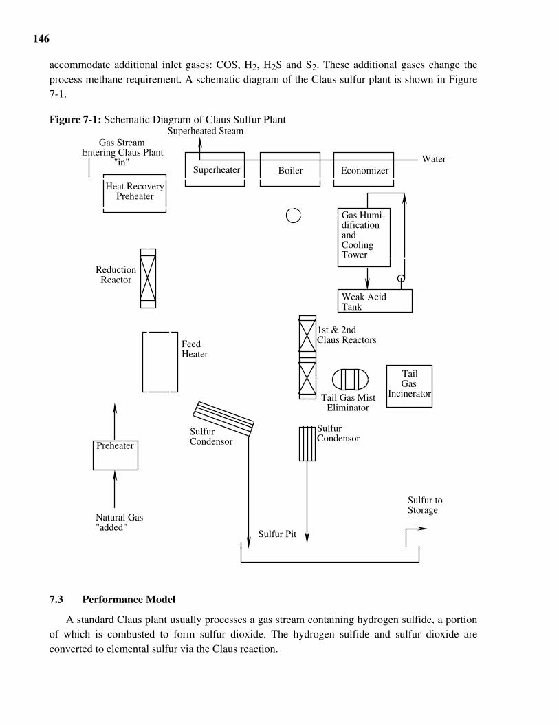
146
accommodate additional inlet gases: COS, H2, H2S and S2. These additional gases change theprocess methane requirement. A schematic diagram of the Claus sulfur plant is shown in Figure7-1.
Figure 7-1: Schematic Diagram of Claus Sulfur Plant
Gas Humi- dification and Cooling Tower
Weak Acid Tank
Heat Recovery Preheater
Superheater Boiler Economizer
Natural Gas "added"
Superheated Steam
Sulfur Condensor
Sulfur Condensor
Tail Gas
Incinerator
1st & 2nd Claus Reactors
Sulfur Pit
Sulfur to Storage
Feed Heater
Tail Gas Mist Eliminator
Reduction Reactor
Gas Stream Entering Claus Plant
"in" Water
Preheater
7.3 Performance Model
A standard Claus plant usually processes a gas stream containing hydrogen sulfide, a portionof which is combusted to form sulfur dioxide. The hydrogen sulfide and sulfur dioxide areconverted to elemental sulfur via the Claus reaction.
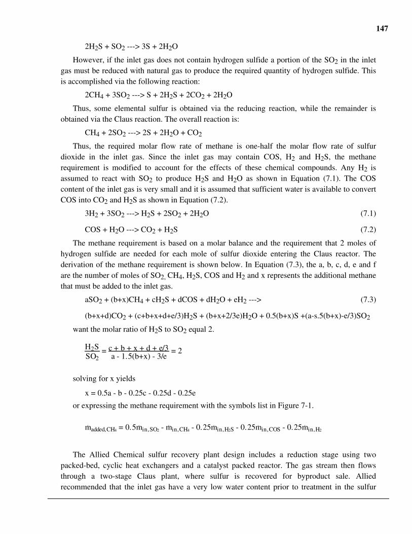
147
2H2S + SO2 ---> 3S + 2H2O
However, if the inlet gas does not contain hydrogen sulfide a portion of the SO2 in the inletgas must be reduced with natural gas to produce the required quantity of hydrogen sulfide. Thisis accomplished via the following reaction:
2CH4 + 3SO2 ---> S + 2H2S + 2CO2 + 2H2O
Thus, some elemental sulfur is obtained via the reducing reaction, while the remainder isobtained via the Claus reaction. The overall reaction is:
CH4 + 2SO2 ---> 2S + 2H2O + CO2
Thus, the required molar flow rate of methane is one-half the molar flow rate of sulfurdioxide in the inlet gas. Since the inlet gas may contain COS, H2 and H2S, the methanerequirement is modified to account for the effects of these chemical compounds. Any H2 isassumed to react with SO2 to produce H2S and H2O as shown in Equation (7.1). The COScontent of the inlet gas is very small and it is assumed that sufficient water is available to convertCOS into CO2 and H2S as shown in Equation (7.2).
3H2 + 3SO2 ---> H2S + 2SO2 + 2H2O (7.1)
COS + H2O ---> CO2 + H2S (7.2)
The methane requirement is based on a molar balance and the requirement that 2 moles ofhydrogen sulfide are needed for each mole of sulfur dioxide entering the Claus reactor. Thederivation of the methane requirement is shown below. In Equation (7.3), the a, b, c, d, e and fare the number of moles of SO2, CH4, H2S, COS and H2 and x represents the additional methanethat must be added to the inlet gas.
aSO2 + (b+x)CH4 + cH2S + dCOS + dH2O + eH2 ---> (7.3)
(b+x+d)CO2 + (c+b+x+d+e/3)H2S + (b+x+2/3e)H2O + 0.5(b+x)S +(a-s.5(b+x)-e/3)SO2
want the molar ratio of H2S to SO2 equal 2.
H2SSO2
= c + b + x + d + e/3a - 1.5(b+x) - 3/e
= 2
solving for x yields
x = 0.5a - b - 0.25c - 0.25d - 0.25e
or expressing the methane requirement with the symbols list in Figure 7-1.
madded,CH4 = 0.5min,SO2 - min,CH4 - 0.25min,H2S - 0.25min,COS - 0.25min,H2
The Allied Chemical sulfur recovery plant design includes a reduction stage using twopacked-bed, cyclic heat exchangers and a catalyst packed reactor. The gas stream then flowsthrough a two-stage Claus plant, where sulfur is recovered for byproduct sale. Alliedrecommended that the inlet gas have a very low water content prior to treatment in the sulfur
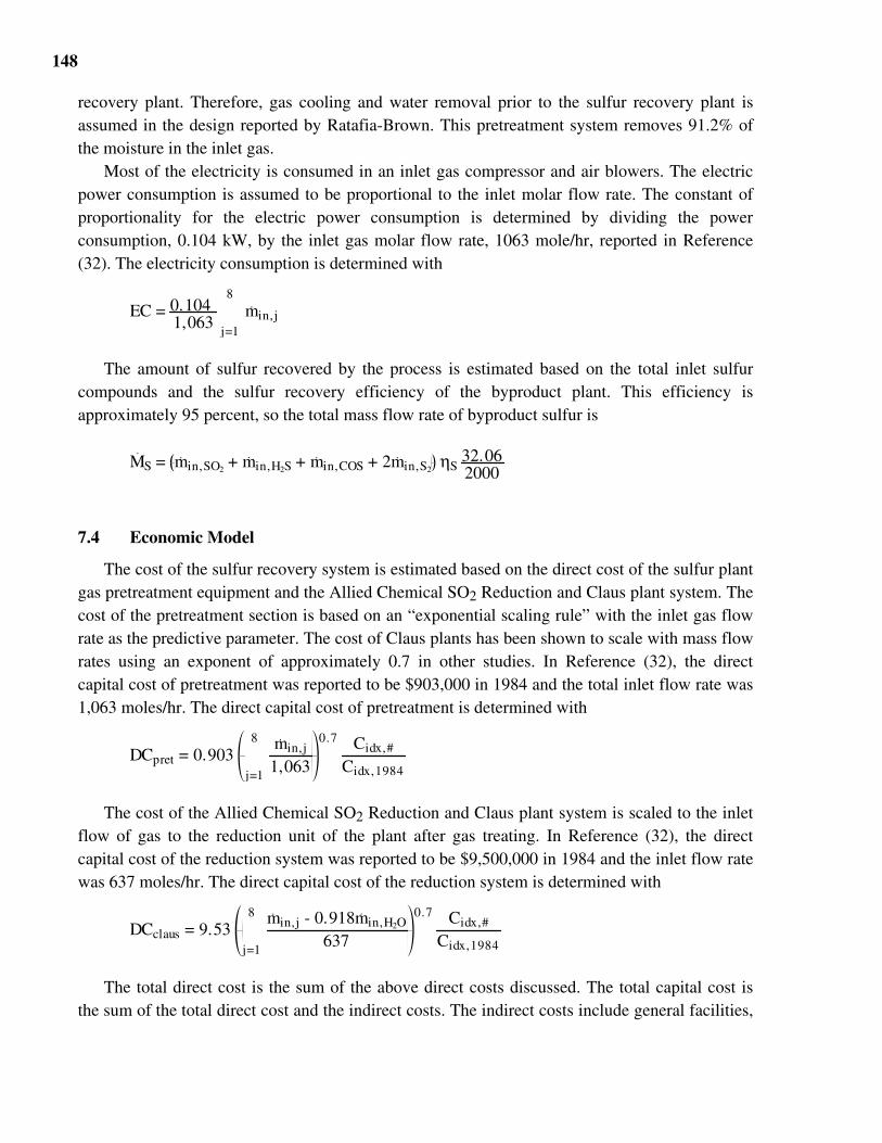
148
recovery plant. Therefore, gas cooling and water removal prior to the sulfur recovery plant isassumed in the design reported by Ratafia-Brown. This pretreatment system removes 91.2% ofthe moisture in the inlet gas.
Most of the electricity is consumed in an inlet gas compressor and air blowers. The electricpower consumption is assumed to be proportional to the inlet molar flow rate. The constant ofproportionality for the electric power consumption is determined by dividing the powerconsumption, 0.104 kW, by the inlet gas molar flow rate, 1063 mole/hr, reported in Reference(32). The electricity consumption is determined with
EC = 0.104 1,063
min,jj=1
8
The amount of sulfur recovered by the process is estimated based on the total inlet sulfurcompounds and the sulfur recovery efficiency of the byproduct plant. This efficiency isapproximately 95 percent, so the total mass flow rate of byproduct sulfur is
MS = min,SO2 + min,H2S + min,COS + 2min,S2
ηS 32.062000
7.4 Economic Model
The cost of the sulfur recovery system is estimated based on the direct cost of the sulfur plantgas pretreatment equipment and the Allied Chemical SO2 Reduction and Claus plant system. Thecost of the pretreatment section is based on an “exponential scaling rule” with the inlet gas flowrate as the predictive parameter. The cost of Claus plants has been shown to scale with mass flowrates using an exponent of approximately 0.7 in other studies. In Reference (32), the directcapital cost of pretreatment was reported to be $903,000 in 1984 and the total inlet flow rate was1,063 moles/hr. The direct capital cost of pretreatment is determined with
DCpret = 0.903 min,j
1,063j=1
8 0.7
Cidx,#
Cidx,1984
The cost of the Allied Chemical SO2 Reduction and Claus plant system is scaled to the inletflow of gas to the reduction unit of the plant after gas treating. In Reference (32), the directcapital cost of the reduction system was reported to be $9,500,000 in 1984 and the inlet flow ratewas 637 moles/hr. The direct capital cost of the reduction system is determined with
DCclaus = 9.53 min,j - 0.918min,H2O
637j=1
8 0.7
Cidx,#
Cidx,1984
The total direct cost is the sum of the above direct costs discussed. The total capital cost isthe sum of the total direct cost and the indirect costs. The indirect costs include general facilities,
149
engineering and home office fees and project and process contingency and are expressed as afraction of the total direct cost.
TDC = DC + DC
TCC = TDC (1 + ICF)
The annual costs of the sulfur recovery plant include methane and power consumption andsulfur by-product credit. The annual costs for methane and power consumption are accounted forin either the copper oxide or NOXSO process. The credit from the sale of the by-product sulfuris:
ACS,credit = 8766x10-6 Cf PS MS
The model does not include costs for catalyst replacement. A typical annual replacement cost isonly a few thousand dollars, negligible compared to the annual totals. However, the initialcatalyst charge is included in the capital costs.
150
8 FROTH FLOTATION PROCESS MODEL
8.1 Nomenclature
A = Ash content coal (fraction)AC = Annual operating cost (78$/dry ton of clean coal)ck = Chemical cost for kth level plant (78$/dry ton of cleaned coal)CS = Concentration of solids (fraction)DC = Direct capital cost (78$)DCC = Cost coefficient for cleaning equipment (78$/dry ton of raw coal)ek = Electricity cost for kth level plant (78$/dry ton of cleaned coal)Ed = Energy needed for thermal drier (Btu/lb of dry coal)f = Weight fraction of coal (fraction)HHV = Average higher heating value of coal (Btu/lb)Kspecie = Rate constant of specie (min-1)lk = Labor cost for kth level plant (78$/dry ton of cleaned coal)LHV = Lower heating value of coal (Btu/lb)m' = Total moisture content of coal (fraction)mi' = Inherent moisture content of coal (fraction)ms' = Surface moisture content of coal (fraction)m = Dry mass flow rate of coal (tons/hr)MIBC = MIBC consumption of froth flotation circuit (lb/raw dry ton)O = #2 fuel oil consumption of froth flotation circuit (lb/raw dry ton)rspecie = Recovery of species (fraction)Rspecie = Ultimate recovery constant of species (fraction)S = Sulfur content of coal (fraction)T = Residence time of flotation vessels (minutes)v = Volume of flotation cells (ft3)Vef = Effective volume of flotation equipment (fraction)w' = Weight of water evaporated in thermal drier per pound of dry coal processed
(fraction)w'e = Weight of water evaporated in thermal drier (tons/hr)wk = Water cost for kth level plant (78$/dry ton of cleaned coal)Yd = Mass yield of the thermal drier (fraction)Yp = Mass yield of coal cleaning plant excluding the thermal drier yield (fraction)Yt = Mass yield of the entire coal cleaning plant (fraction)Yod = Ratio of coal mass exiting wash streams to coal mass exiting plant (fraction)
Greek Letter Symbolsε = Efficiency of thermal drier (fraction)δi = Equals 0 if wash stream i is not thermally dried and 1 if it is thermally dried.ρc = density of coal (lb/ft3)ρw = density of water (lb/ft3)
Subscripts:c = clean coal exiting wash streamsd = thermal drieri = (1) coarse, (2) medium or (3) fine streamsin = entering thermal drierj = oil or MIBC
151
k = level of plant (2,3,4 or 5)l = clean, thermal, raw, refuse, sampleo = clean coal exiting plantout = exiting thermal drierref = refuse coalROM = raw coal
species:a = ashafc = ash-free coals = sulfur content
8.2 Introduction
This chapter describes the addition of a conventional froth flotation circuit into the coalcleaning module of the IECM. The purpose of this modification is to include froth flotation as anoption to clean the fine coal stream. The original model (1) has three beneficiation levels (2, 3and 4) in which different streams are washed by specific gravity equipment. Level 2 washes onlythe coarse stream. Level 3 washes the coarse and medium streams. Level 4 washes the coarse,medium and fine streams. The new modification adds a fifth level, which uses specific gravityequipment to wash the coarse and medium streams and froth flotation equipment for the finestream. The specific size fractions in each stream are specified by the model user. As before, themodel optimizes the yield of each circuit To achieve a target coal quality for the cleaned coalproduct.
8.3 Process Description
This section only briefly describes froth flotation of coal. For a more detailed descriptions ofthe froth flotation process see References (37-41). Most coal cleaning processes use thedifference between the specific gravity of coal, ash and pyrite to separate the coal from the ashand pyrite (40). Froth flotation, however, uses the difference between the adhesion of small airbubbles to coal, ash and pyrite to achieve separation. Usually small air bubbles are passedthrough a fine coal slurry stream. Air attaches itself to coal and floats to the surface, where it isremoved. Since the air does not attach itself to the ash it remains in the slurry and is carried off.Particles which stick to air bubbles are called hydrophobic, while those which are easily wettedare called hydrophilic.
Coal is inherently hydrophobic, but the degree of floatability depends on several parameters,including particle size, pulp density, coal rank, extent of oxidation, quantity and type ofchemicals used, slurry pH, aeration and agitation, retention time. Three theories which broadlytry to predict the floatability of coal are the carbon-hydrogen ratio theory, the carbon contenttheory and the surface-components theory. All three theories have advantages and disadvantagesin predicting the floatability of coal. Yet, none of the theories predicts the quality and yield ofcoal for a specific set of flotation parameters. Although they are not applicable for this model,they can be used to estimate the performance of a new coal from existing floatability data.
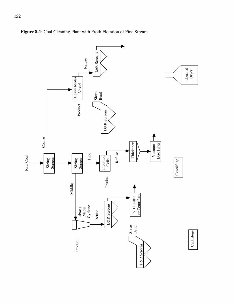
152
Figure 8-1: Coal Cleaning Plant with Froth Flotation of Fine StreamR
aw C
oal
Coa
rse
Mid
dle
Fine
D&
R S
cree
ns
Sizi
ng
Scre
ens
Sizi
ng
Scre
ens
Hea
vy M
edia
V
esse
l
D&
R S
cree
ns
Hea
vy
Med
ia
Cyc
lone
Flo
tati
on
Cel
ls Ref
use
Ref
use
Ref
use
Pro
duct
Pro
duct
Pro
duct
Thi
cken
er
Vac
uum
D
isc
Filte
r
V.D
. Filt
er
or C
entr
ifug
e
Cen
trif
uge
Cen
trif
uge
The
rmal
D
ryer
D&
R S
cree
ns
D&
R S
cree
ns
Siev
e B
end
Siev
e B
end
153
Usually chemicals, called frothers, are added to the coal slurry to prolong the life of the airbubbles, which enhances the stability of the froth. MIBC (methyl isobutyl carbinol) is a commonfrother used for coal froth flotation. Collectors increase the adhesion of air to coal and are neededfor highly oxidized or lower rank coals. A common collector used for froth flotation of coal isfuel oil. Other chemicals can be added which perform a variety of functions. The most commonare depressing agents, activating agents, pH regulators, dispersing agents and protective colloids.
Figure 8-1 shows the a process diagram for a conventional coal cleaning plant with frothflotation for the fine size stream. Although it is widely used, the process is not understood as wellas specific gravity based beneficiation. Because less is known about froth flotation, it is difficultto predict full scale performance from laboratory batch data. Although there are algorithms forscaling up laboratory data (42), they have not been implemented in this model until they can befurther evaluated. It is also generally accepted that flotation washability data cannot be predictedfrom specific gravity washability data (43, 44).
8.4 Froth Flotation Performance Model
A complete description of the conventional coal cleaning model is found in Reference (1).This report only discusses the improvements that have been added. The model uses a Lagrangemultiplier technique to maximize the yield (mass or energy) for a given coal and plantconfiguration. The algorithm needs discrete data points of the yield and coal quality at differentspecific gravities for three wash streams (coarse, medium, fine). For froth flotation of the finesizestream, the user can specify washability data in one of three different ways:
• Actual yield and quality data at different residence times• Rate and ultimate recovery constants for ash-free yield, ash and sulfur content• Mass yield and coal quality of the cleaned coal for the flotation circuitFor all three options the following information is also needed:• The quantity of MIBC and #2 fuel oil,• Inlet slurry concentration• Effective volume of the cellsFor option one, the froth flotation data is substituted for the conventional fine stream data and
the model optimizes the yield for all three streams as usual. Data in this form can be found inReference 9. But, this is batch data and has not been scaled to full size. The only difference isthat the residence time is determined instead of a specific gravity for the fine stream. The onlyrestriction currently is that the number of coal quality data points for froth flotation must equalthe number of specific gravity data points.
For the second option, the rate and ultimate recovery constants are used in the Klimpel model(Equation 8.1) to predict the recovery of ash-free coal, ash and sulfur at different residencestimes (42, 43):
ri = Ri 1 - 1KiT
1 - e-KiT (8.1)
154
The total mass yield is equal to the sum of the ash-free coal and ash recovered (Equation 8.2).The ash content of the cleaned coal is equal to the recovery of ash times the raw coal ash contentdivided by the mass yield (Equation 8.3). The sulfur content of the cleaned coal is determinedsimilarly (Equation 8.4). The higher heating value is estimated by Equation 8.5.
Yp,3 = (1 - AROM) rafc + AROMra (8.2)
Ao,3
= Y
p,3
AROM
ra (8.3)
So,3 = Yp,3
SROMrs (8.4)
HHVo,3
= HHVROM
1 - A
ROM
1 - Ao,3
(8.5)
The coal yield and quality in the froth circuit at different residence intervals can bedetermined with Equations 8.2 - 8.5. The residence times intervals are determined by specifyinga maximum residence time and dividing by the number of specific gravity data points.19 Thisdata is then substituted into the fine size washability data and the model proceeds as usual.
For the third option, the yield and quality of the froth flotation circuit is specified at a givenresidence time. This data is passed into the optimization algorithm, where the model optimizesthe mass yields of the coarse and medium streams to achieve the overall target coal quality.
For all three options, once the residence time is determined the total volume of the cells canbe determined from Equation 8.6:
v = mROM fROM,3
T 60 min/hr
2000 lb/ton r c
1 + CS
1 - 1 r w
1 V
ef
1 (8.6)
The densities of water and coal are assumed to be 84 and 62 lb/ft3, respectively. Theeffective volume, Vef, is used to account for the volume occupied by the air-ingestion equipmentand air bubbles.
8.5 Process Economics
The general coal cleaning plant economic model is based on several studies (45-50) and isdescribed in Reference (1). All cost are computed in 1978 dollars then escalated to a current yearusing a plant cost index. The same method is used to estimate the cost of the new level five plantwith froth flotation. The capital cost is divided into five different sections: (1) raw coal handling,
19 This will be changed to the maximum number of data points possible in the next version of the model.
155
(2) cleaning equipment, (3) thermal drying, (4) refuse handling and (5) coal sampling system.The direct capital cost of each section other than the coal sampling system is related to itscharacteristic mass flow and is assumed to have an economy of scale of 0.7 for plant sizes in therange of 500 to 2000 clean tons per hour (tph) (46). Only the cost of the cleaning equipmentsection is assumed to vary with different levels of coal cleaning. The capital cost related to cleancoal handling (which includes the cost of conveyors, storage and loading equipment) is includedin the raw coal handling cost since the cleaning plant is assumed to be at the mine site. It isassumed that the cost of the coal sampling system does not vary with plant capacity.
The economics of froth flotation depend on the residence time, chemical usage and processyield. The direct capital for the cleaning equipment for a level 5 plant is estimated by Equation8.7:
DCclean = DCC5 mROM0.7 + 6780 v0.4 (8.7)
where DCC5 = 43,700
The first term of Equation 8.7 is the capital cost of the cleaning equipment excluding theflotation cells. The second term is the capital cost of the flotation cells. The value for the firstterm was obtained from Reference (46). It represents the average cost of cleaning equipmentexcluding the flotation cells scaled to the raw coal mass flow rate. The direct capital cost for thefroth flotation equipment is scaled to the total volume of the vessels (46, 47). An exponentialscaling factor of 0.4 is used as the best fit to available data (46, 47).
The indirect and annualized capital costs are calculated as shown in Reference (1). Theoperating and maintenance costs of a level five plant are calculated similarly to the other levels.The cost factors for labor, maintenance, refuse and taxes are the same as a level four plant (46).The cost factor for chemicals (excluding oil and MIBC), electricity and water are, respectively,0.064, 0.15 and 0.0015 in 1978$/ton of raw coal (45). The amounts of MIBC and #2 fuel oil usedare input parameters in the model. Therefore, the cost per ton of cleaned coal is estimated by thefollowing equations:
ACoil
= Yt
0.072 O fROM,3
ACMIBC
= Yt
0.60 MIBC fROM,3
156
9 SELECTIVE AGGLOMERATION PROCESS MODEL
9.1 Nomenclature
English SymbolsAclean Ash content of the clean coal going to thermal drier (fraction)Ar Ash content of the raw coal input (fraction)Aref Ash content of the refuse coal (fraction)ACelect Annual cost of electricity ( $ / dry ton of cleaned coal)AClabor Annual cost of labor ( $ / dry ton of cleaned coal)ACagg Annual cost of agglomerant ( $ / dry ton of cleaned coal)ACmaint Annual cost of maintenance ( $ / dry ton of cleaned coal)ACpayovh Annual cost of payroll overheads ( $ / dry ton of cleaned coal)ACplovh Annual cost of plant overheads ( $ / dry ton of cleaned coal)ACtax Annual cost of taxes, insurance, etc ( $ / dry ton of cleaned coal)ACwaste Annual cost of waste disposal ( $ / dry ton of cleaned coal)ACwater Annual cost of water ( $ / dry ton of cleaned coal)c Cost of agglomerant used ($/lb agglomerant)Cidx Chemical engineering cost indexCidx, 1984 Chemical engineering cost index for 1984 for current yearCsol Degree of agglomerant solubility in water (fraction)Ccapital Total capital cost ($ /dry ton of cleaned coal)Coperating Total operating cost ($ /dry ton of cleaned coal)Cr Cost of raw coal ($ /dry ton of raw coal)Cref Cost of refuse coal ($ /dry ton of cleaned coal)Ctotal Total cost of clean coal ($ /dry ton of cleaned coal)CRF Capital Recovery factor (dimensionless)d Real discount rate for capital cost (fraction)DC Direct capital cost ($)DCaggequip Direct capital cost of the selective agglomeration plant equipment ($)DCaggrec Direct capital cost of agglomerant recovery equipment ($)DCr Direct capital cost of the refuse handling ($)DCref Direct capital cost of the refuse handling ($)DCthermal Direct capital cost of thermal drying system ($)e Cost of electricity ($/dry ton of raw coal)Edrier Energy needed for thermal drier (Btu)h Annual operating hours of coal cleaning plant (hrs/yr)HHVr Higher heating value of raw coal (Btu/lb dry coal)HHVclean Higher heating value of raw coal (Btu/lb dry coal)i Nominal interest rate (fraction)l Labor cost ($/hr)LHV Lower heating value of cleaned coal (Btu/lb dry coal)mdry Dry mass flow rate of clean coal entering the thermal drier (tons/hr)mevapwater Mass flow rate of water evaporated in thermal drier (tons/hr)mevapwater’ Weight of water evaporated in thermal drier per pound of clean coal (fraction)minmois’ Moisture content of clean coal entering thermal drier (fraction)maggclean Mass flow rate of agglomerant entering the evaporator system (tons/hr)magglosttoatmtotMass flow rate of total agglomerant lost to the atmosphere (tons/hr)magglosttowater Mass flow rate of agglomerant lost to water (tons/hr)
157
magglosttosolid Mass flow rate of agglomerant lost to solid(tons/hr)maggnew Mass flow rate of new agglomerant (tons/hr)maggrec Mass flow rate of recovered agglomerant (tons/hr)maggtotal Mass flow rate of recovered agglomerant mixed with raw coal (tons/hr)mo Dry mass flow rate of clean coal leaving the plant (tons/hr)moutmois’ Moisture content of clean coal leaving thermal drier (fraction)mr Dry mass flow rate of raw coal input (tons/hr)mref Dry mass flow rate of refused coal (tons/hr)msteam Total mass flow rate of steam required for stripping system (tons/hr)mwater Total mass flow rate of cooling water required for stripping system (tons/hr)mt Cost of maintenance (fraction)n Life of coal cleaning plant (years)p Inflation rate (fraction)PSclean Pyritic sulfur in the clean coal removed from the raw input (%)r Cost of refuse coal disposal ($/wet ton)R Ratio of dry mass agglomerant to dry mass of raw coal (dimensionless)s Cost of steam ($/1000 tons)t Annual rate of taxes and insurance costs for plant (fraction)TCC Total capital cost ($)TDC Total direct capital costw Cost of water ($/1000 tons)W Water loss in the process (tons/hr)Wc Working capital ($/dry of clean coal)Yclean Mass yield of clean coal going to the thermal drier (fraction)Ydrier Thermal drier mass yield (fraction)Ytotal Mass yield of entire coal cleaning plant (fraction)
Greek letter symbols ε Efficiency of thermal drier (fraction)
9.2 Introduction
This chapter presents new performance and economic models simulating the operation of acoal beneficiation plant using the selective agglomeration process. The primary function of thismodel is to estimate the cost and ability of the process to remove the pyritic sulfur and ash tohelp meet power plant emission standards. This section presents a brief overview of the selectiveagglomeration process, a description of the economic algorithms and an assessment of thisprocess’ ability to reduce sulfur dioxide emissions of coal fired power plants. Performancemodels are based on bench-scale tests on a one ton per hour (tph) Proof-of-Concept (POC) unitperformed by Bechtel for the U.S Department of Energy, Pittsburgh Energy Technology Centerunder Contract No. DE-AC-22-84PC79867 (51). An assessment of capital investment andoperating costs for a selective agglomeration process with plant size of 300 tph proposed byBurns and Roe Services Corporation is adopted in developing the economic model (52).
In selective coalescence (also known as selective agglomeration), an agglomerating liquidsuch as chlorofluorocarbons (e.g., Freon 113) or hydrocarbons (e.g., n-pentane and n-heptane) iscontacted with an agitated, aqueous suspension of the feed coal. The coal particles agglomerateinto a large floc in the non-aqueous phase. The mineral matter particles which remain dispersedin the aqueous phase are then separated by screening the flocs.
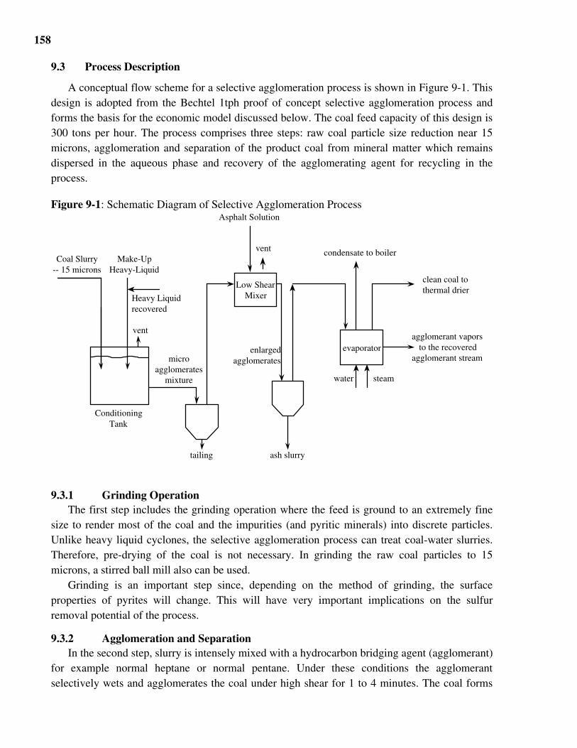
158
9.3 Process Description
A conceptual flow scheme for a selective agglomeration process is shown in Figure 9-1. Thisdesign is adopted from the Bechtel 1tph proof of concept selective agglomeration process andforms the basis for the economic model discussed below. The coal feed capacity of this design is300 tons per hour. The process comprises three steps: raw coal particle size reduction near 15microns, agglomeration and separation of the product coal from mineral matter which remainsdispersed in the aqueous phase and recovery of the agglomerating agent for recycling in theprocess.
Figure 9-1: Schematic Diagram of Selective Agglomeration Process
Coal Slurry
-- 15 microns Make-Up
Heavy-Liquid
Low Shear Mixer Heavy Liquid
recovered
Conditioning Tank
tailing
Asphalt Solution
micro agglomerates
mixture
enlarged agglomerates
evaporator
steam
clean coal to thermal drier
agglomerant vapors to the recovered
agglomerant stream
condensate to boiler
water
ash slurry
vent
vent
9.3.1 Grinding OperationThe first step includes the grinding operation where the feed is ground to an extremely fine
size to render most of the coal and the impurities (and pyritic minerals) into discrete particles.Unlike heavy liquid cyclones, the selective agglomeration process can treat coal-water slurries.Therefore, pre-drying of the coal is not necessary. In grinding the raw coal particles to 15microns, a stirred ball mill also can be used.
Grinding is an important step since, depending on the method of grinding, the surfaceproperties of pyrites will change. This will have very important implications on the sulfurremoval potential of the process.
9.3.2 Agglomeration and SeparationIn the second step, slurry is intensely mixed with a hydrocarbon bridging agent (agglomerant)
for example normal heptane or normal pentane. Under these conditions the agglomerantselectively wets and agglomerates the coal under high shear for 1 to 4 minutes. The coal forms
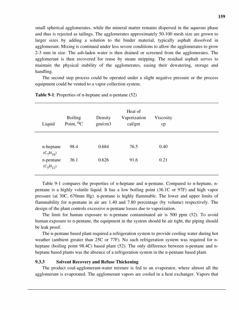
159
small spherical agglomerates, while the mineral matter remains dispersed in the aqueous phaseand thus is rejected as tailings. The agglomerates approximately 50-100 mesh size are grown tolarger sizes by adding a solution to the binder material, typically asphalt dissolved inagglomerant. Mixing is continued under less severe conditions to allow the agglomerates to grow2-3 mm in size. The ash-laden water is then drained or screened from the agglomerates. Theagglomerant is then recovered for reuse by steam stripping. The residual asphalt serves tomaintain the physical stability of the agglomerates, easing their dewatering, storage andhandling.
The second step process could be operated under a slight negative pressure or the processequipment could be vented to a vapor collection system.
Table 9-1: Properties of n-heptane and n-pentane (52)
Heat ofBoiling Density Vaporization Viscosity
Liquid Point, oC gm/cm3 cal/gm cp
n-heptane 98.4 0.684 76.5 0.40 (C7H16)
n-pentane 36.1 0.626 91.6 0.21 (C5H12)
Table 9-1 compares the properties of n-heptane and n-pentane. Compared to n-heptane, n-pentane is a highly volatile liquid. It has a low boiling point (36.1C or 97F) and high vaporpressure (at 30C, 670mm Hg). n-pentane is highly flammable. The lower and upper limits offlammability for n-pentane in air are 1.40 and 7.80 percentage (by volume) respectively. Thedesign of the plant controls excessive n-pentane losses due to vaporization.
The limit for human exposure to n-pentane contaminated air is 500 ppm (52). To avoidhuman exposure to n-pentane, the equipment in the system should be air tight, the piping shouldbe leak proof.
The n-pentane based plant required a refrigeration system to provide cooling water during hotweather (ambient greater than 25C or 77F). No such refrigeration system was required for n-heptane (boiling point 98.4C) based plant (52). The only difference between n-pentane and n-heptane based plants was the absence of a refrigeration system in the n-pentane based plant.
9.3.3 Solvent Recovery and Refuse ThickeningThe product coal-agglomerant-water mixture is fed to an evaporator, where almost all the
agglomerant is evaporated. The agglomerant vapors are cooled in a heat exchanger. Vapors that
160
are not condensed are compressed by a compressor. The resulting liquid is circulated to theconditioning tank. The product coal may retain as little as 50 to 100 ppm of the agglomerant.
The product coal can be obtained as a somewhat dry product containing 10% moisture or as apulp containing 40% water. This will depend on the type of evaporator used to vaporize theagglomerant.
The mineral matter-water slurry contains very small amount of agglomerant (50 to 100 ppm).This slurry is thickened in a static thickener and the clarified water is recirculated to the circuitand the refuse is sent to the refuse disposal circuit.
9.4 Performance Model
The selective agglomeration process was evaluated by Bechtel for three coals. They arePittsburgh No.8, Illinois No.6 and Upper Freeport seams. The average ROM coal characteristicsfor these coals are shown in Table 9-2. Using Bechtel’s 1tph POC, the average clean coalperformance for coal plants of 300 tph (dry) coal feed is estimated and shown in Table 9-2.
It was not possible to develop a generalized algorithm which would determine the quality andyield of the clean coal based on the experimental data. Therefore, the model uses experimentaldata of the cleaned coals quality (i.e. ash and sulfur content) and mass yield directly to determinethe cost of the cleaned coal. The input parameters for the performance and economic models are:
• Ash, sulfur, inherent moisture and surface moisture contents of raw coal• Higher heating value of raw coal• Ash, sulfur, surface moisture of cleaned coal• Mass yield of process• Moisture content entering thermal drier• Mass ratio of agglomerant to dry raw coal• Solubility of agglomerant in water• Efficiency of thermal drier• Cost of agglomerant in dollars per tonAs noted above, the basic performance parameters characterizing the change in coal quality
are determined from experimental data for a particular coal. Because data for the selectiveagglomeration process are currently limited, only three coals are represented here.
If the higher heating value of the clean coal is not provided then the following algorithm isused
HHVclean = (HHV)r [1-Aclean]/[1-Araw]
Estimates of plant operating and capital costs typically are scaled to various mass flow rateswithin the coal cleaning plant. Those developed below are the rate of raw coal and agglomerantinto the plant, the rate of dry and wet refuse coal out of the plant, the rate of agglomerantrecovered and lost from the plant, the rate steam and water required for stripping the agglomerantand the rate of water evaporated in the thermal drier. The process flow scheme with respectivemass flows shown in Figure 9-2.
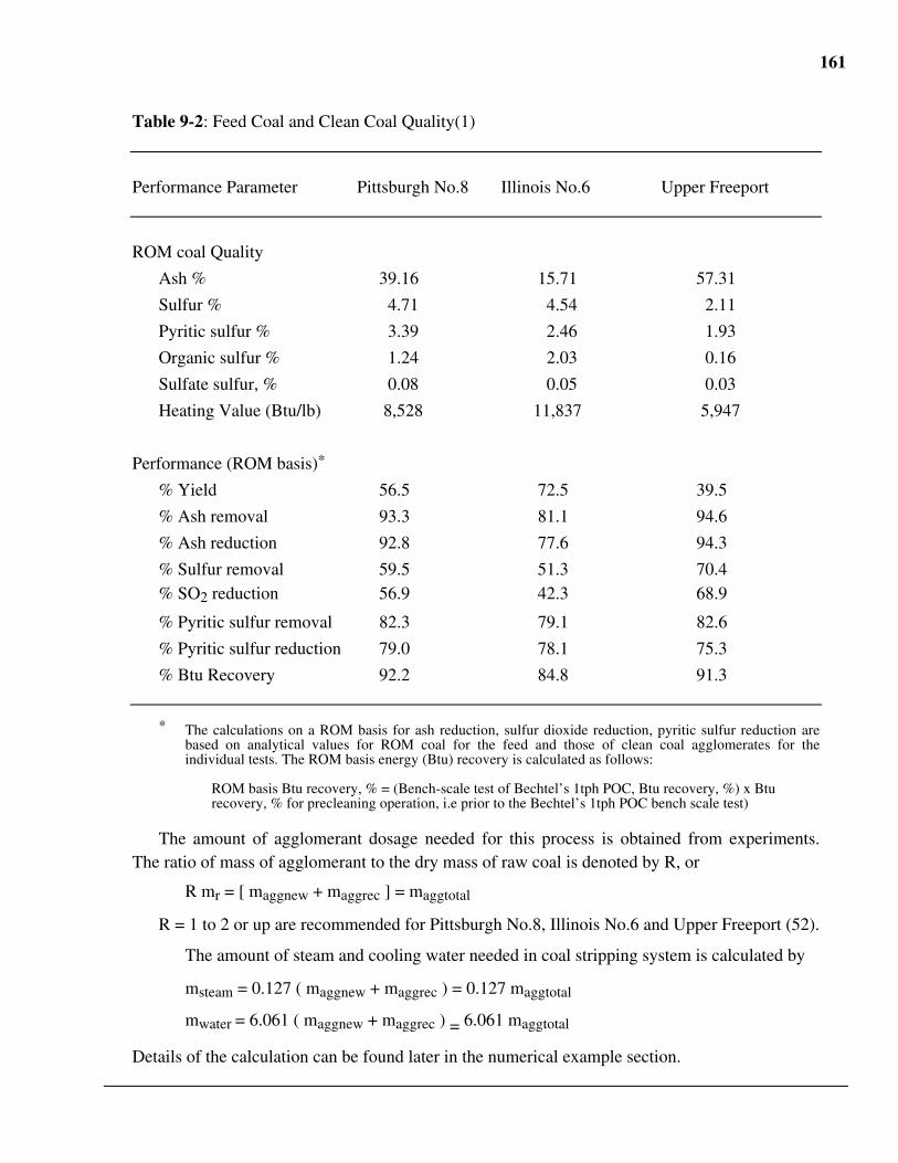
161
Table 9-2: Feed Coal and Clean Coal Quality(1)
Performance Parameter Pittsburgh No.8 Illinois No.6 Upper Freeport
ROM coal Quality
Ash % 39.16 15.71 57.31
Sulfur % 4.71 4.54 2.11
Pyritic sulfur % 3.39 2.46 1.93
Organic sulfur % 1.24 2.03 0.16
Sulfate sulfur, % 0.08 0.05 0.03
Heating Value (Btu/lb) 8,528 11,837 5,947
Performance (ROM basis)*
% Yield 56.5 72.5 39.5
% Ash removal 93.3 81.1 94.6
% Ash reduction 92.8 77.6 94.3
% Sulfur removal 59.5 51.3 70.4% SO2 reduction 56.9 42.3 68.9
% Pyritic sulfur removal 82.3 79.1 82.6
% Pyritic sulfur reduction 79.0 78.1 75.3
% Btu Recovery 92.2 84.8 91.3
* The calculations on a ROM basis for ash reduction, sulfur dioxide reduction, pyritic sulfur reduction arebased on analytical values for ROM coal for the feed and those of clean coal agglomerates for theindividual tests. The ROM basis energy (Btu) recovery is calculated as follows:
ROM basis Btu recovery, % = (Bench-scale test of Bechtel’s 1tph POC, Btu recovery, %) x Bturecovery, % for precleaning operation, i.e prior to the Bechtel’s 1tph POC bench scale test)
The amount of agglomerant dosage needed for this process is obtained from experiments.The ratio of mass of agglomerant to the dry mass of raw coal is denoted by R, or
R mr = [ maggnew + maggrec ] = maggtotal
R = 1 to 2 or up are recommended for Pittsburgh No.8, Illinois No.6 and Upper Freeport (52).
The amount of steam and cooling water needed in coal stripping system is calculated by
msteam = 0.127 ( maggnew + maggrec ) = 0.127 maggtotal
mwater = 6.061 ( maggnew + maggrec ) = 6.061 maggtotal
Details of the calculation can be found later in the numerical example section.
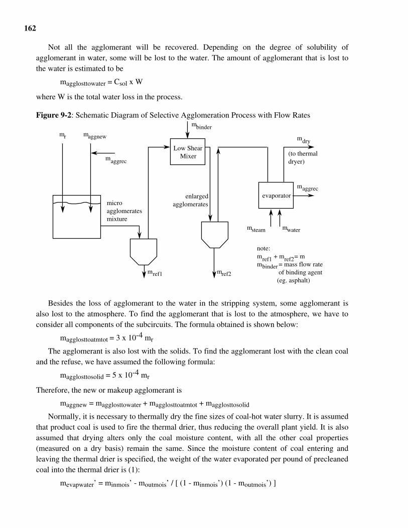
162
Not all the agglomerant will be recovered. Depending on the degree of solubility ofagglomerant in water, some will be lost to the water. The amount of agglomerant that is lost tothe water is estimated to be
magglosttowater = Csol x W
where W is the total water loss in the process.
Figure 9-2: Schematic Diagram of Selective Agglomeration Process with Flow Rates
Low Shear Mixer
micro agglomerates mixture
enlarged agglomerates
evaporator
mdry
maggrec
msteam mwater
mref2mref1
mr maggnew
maggrec
mbinder
(to thermal dryer)
note: m + m = m m = mass flow rate of binding agent (eg. asphalt)
ref1 ref2binder
Besides the loss of agglomerant to the water in the stripping system, some agglomerant isalso lost to the atmosphere. To find the agglomerant that is lost to the atmosphere, we have toconsider all components of the subcircuits. The formula obtained is shown below:
magglosttoatmtot = 3 x 10⁻⁴ mr
The agglomerant is also lost with the solids. To find the agglomerant lost with the clean coaland the refuse, we have assumed the following formula:
magglosttosolid = 5 x 10⁻⁴ mr
Therefore, the new or makeup agglomerant is
maggnew = magglosttowater + magglosttoatmtot + magglosttosolid
Normally, it is necessary to thermally dry the fine sizes of coal-hot water slurry. It is assumedthat product coal is used to fire the thermal drier, thus reducing the overall plant yield. It is alsoassumed that drying alters only the coal moisture content, with all the other coal properties(measured on a dry basis) remain the same. Since the moisture content of coal entering andleaving the thermal drier is specified, the weight of the water evaporated per pound of precleanedcoal into the thermal drier is (1):
mevapwater’ = minmois’ - moutmois’ / [ (1 - minmois’) (1 - moutmois’) ]
163
The amount of energy needed to evaporate this water is
Ed = 1020 mevapwater’ / ε
The lower heating value can be approximated by
LHV = 0.96 HHVclean - [ 1020 moutmois’ / ( 1 - moutmois’ ) ]
Therefore, the drier yield and total plant yield are given by
Ydrier = 1 - Ed / LHV
and
Ytotal = YcleanYdrier
The weight of water evaporated is
mevapwater = mevapwater’ [ mdry / Ydrier ]
Once the drier is determined, the dry mass flow rates for the raw coal stream, refuse streamand drier stream can be calculated by the following equations:
mr = mo / Ytotal
mdry = mo / Ydrier
mref = mr - mdry
The water loss in the coal cleaning plant is
W = mdry [ ( 1 / ( 1 - minmois’)) -1] + mref [ ( 1 / RC ) - 1 ]
9.5 Economic Model
The total cost in dollars per ton of dry cleaned coal can be divided into four separate costscategories.
• cost of raw coal• cost of rejected coal• annual operating and maintenance costs• annualized capital costsThe cost of raw coal is an input parameter. The cost of the refuse coal is a function of the
plant yield and can be calculated from
Cref = Cr [(1/Ytotal ) - 1] (9.1)
9.5.1 Capital CostThe capital cost is divided into five different sections: raw coal handling, selective
agglomeration process equipment, agglomerant handling, refuse handling and thermal driers. Thecapital costs related to clean coal storage is included in the raw coal cost, since the coal cleaningequipment is assumed to be at the mine site. This include the cost for conveyors, storage andloading equipment.The raw coal cost also includes the cost of grinding the ROM feed coal. Thedirect capital cost for refuse handling includes refuse sump and explosion proof pump. The directcapital cost is determined by these equations:
164
DCr = $ 91,963 mr0.7 x Cidx / Cidx,1984
(9.2)
DCaggequip = $10,521mr0.7 x Cidx / Cidx,1984
(9.3)
DCaggrec = $ 102,005 mr0.7 x Cidx/Cidx, 1984
= $ 102,005 x [ (maggnew + maggrec ) / R ]0.7 x Cidx/Cidx, 1984
= $ 102,005 R -0.7(maggnew + maggrec )0.7 x Cidx/Cidx, 1984
(9.4)
DCref = $19,100 mref0.7 x Cidx/Cidx, 1984
(9.5)
DCcoalsampling = $324,000 x Cidx/Cidx, 1984(9.6)
DCdrier = $153, 000 mevapwater0.7 x Cidx/Cidx, 1984
(9.7)
The direct capital cost for the selective agglomeration subcircuit equipment covers the costfor the 18,000 gallon conditioning tank with a carbon steel agitator of 100 horsepower, explosionproof feed pump, 12,000 gallon high shear mixer with stainless steel agitator of 400 horsepower,enclosed sieve bend and a stainless steel horizontal-tube evaporator. The direct cost foragglomerant recovery subcircuit equipment consists of the costs for 12,000 and 500 gallonweathered carbon steel tanks, explosion proof pumps, adsorption tower, blower, sump and 8900ton refrigeration system.
The total direct capital cost is found by adding Equation (9.2) through (9.7)
TDC = DCr + DCaggequip + DCaggrec + DCref + DCdrier + DCcoal sampling
The indirect capital and contingencies costs are estimated to be 54% of the direct capital cost.Therefore, the total capital cost, which is depreciated over the life of the plant is
TCC = 1.54 TDC
The total capital cost is annualized as follows:
d = [ ( 1 + i ) / ( 1 + p ) - 1 ]
Where i is the interest rate and p is the inflation rate. Therefore, capital recover factor is
CRF = d / [ 1 - ( 1 + d )-n ]
Working capital is estimated to be 25% of the labor, maintenance, electricity, water, waste
disposal and chemical(agglomerant) costs as in the conventional plant model described in
Chapter 2.
Wc = 0.25 ( AClabor + ACmaint + ACelect + ACwater + ACwaste + ACagg )
As in Chapter 2, the capital cost in ($ per dry ton of cleaned coal) is
Ccapital = dWc + [ ( TCC x CRF ) / ( mo x h ) ] (9.8)
165
9.5.2 Operating and Maintenance CostThe annual operating and maintenance costs comprise several cost elements, including labor,
maintenance, raw material and waste disposal costs, also taxes, insurance and generaladministrative overhead. The operating and maintenance cost is broken down into thecomponents shown in Table 9-3. The total annual cost of agglomerant in $/ton of clean coal isthen estimated to be:
ACagg = cmaggnew / mo
The cost of labor is estimated to be dependent of plant size. Maintenance costs, taxes andinsurance are estimated to be proportional to the total capital cost of the plant. The cost ofelectricity is linked to the mass flow rate of the coal entering the plant, while the cost of wastedisposal is proportional to the quantity of coal rejected. The cost for water is proportional to theamount of water in the clean coal and refuse streams. Overhead costs are based on labor,maintenance and agglomerant costs. The equations for these costs are:
ACelect = e / Ytot . Cidx / Cidx,1980
AClabor = l / m o . Cidx / Cidx,1980
ACmaint = [ mt. TCC ] / [ mo h ]
ACpayovh = 0.30 AClabor
ACpltovh = 0.26 [ AClabor+ ACmaint+ ACagg ]
ACsteam = smsteam / Ytot . Cidx / Cidx,1980
ACtax = [ t TCC ] / [ mo h ]
ACwaste = [ r mref ] / mo RC . Cidx / Cidx,1980
ACwater = [ w 240 W ] / mo . Cidx / Cidx,1980
where e, l, m, r and w are taken from Table 9-3. Adding the above equations yields and
converting to a base year yield
Coperating = (ACagg + ACelect + AClabor + ACmaint + ACpayovh + ACpltovh
+ ACtax + ACwaste + ACwater ) (9.9)
The total cost for cleaned coal is found by adding Equations (9.1), (9.8), (9.9) and the raw coal
cost
Ctotal = Cr + Cref + Coperating + Ccapital
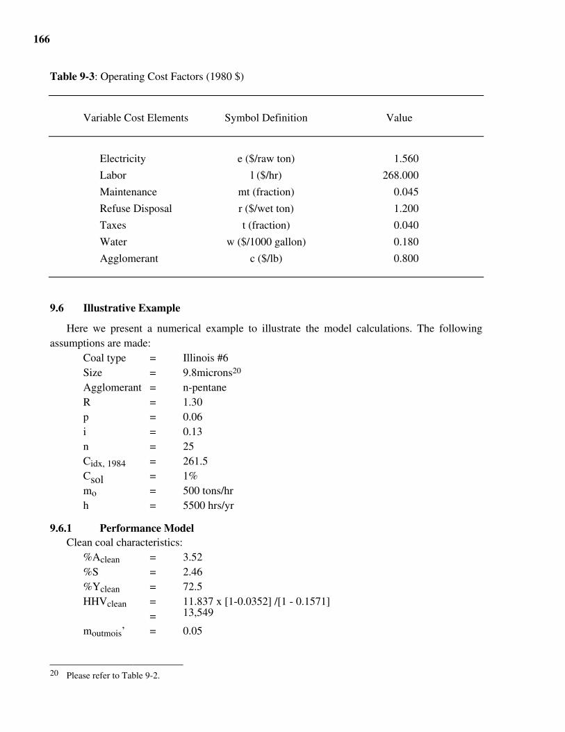
166
Table 9-3: Operating Cost Factors (1980 $)
Variable Cost Elements Symbol Definition Value
Electricity e ($/raw ton) 1.560
Labor l ($/hr) 268.000
Maintenance mt (fraction) 0.045
Refuse Disposal r ($/wet ton) 1.200
Taxes t (fraction) 0.040
Water w ($/1000 gallon) 0.180
Agglomerant c ($/lb) 0.800
9.6 Illustrative Example
Here we present a numerical example to illustrate the model calculations. The followingassumptions are made:
Coal type = Illinois #6Size = 9.8microns20
Agglomerant = n-pentaneR = 1.30p = 0.06i = 0.13n = 25Cidx, 1984 = 261.5Csol = 1%mo = 500 tons/hrh = 5500 hrs/yr
9.6.1 Performance ModelClean coal characteristics:
%Aclean = 3.52%S = 2.46%Yclean = 72.5HHVclean = 11.837 x [1-0.0352] /[1 - 0.1571]
= 13,549
moutmois’ = 0.05
20 Please refer to Table 9-2.
167
Assume minmois’ = 0.24 . Then, the weight of water evaporated per pound of dry intothermal coal drier:
mevapwater’ = [minmois’ - moutmois’] / [ ( 1 - minmois’ ) ( 1 - moutmois’ ) ]= 0.24 - 0.05 / [ ( 1 - 0.24 ) ( 1 - 0.05 ) ]= 0.26
The amount of energy needed to evaporate this water isEd = 1020 mevapwater’ / ε
= [1020 x 0.26] / 0.55 = 482.2 Btu/lbThe lower heating value:
LHV = 0.96 HHVclean - [ (1020 moutmois’ ) / ( 1 - moutmois’ ) ]= 0.96 x 13,549 - [ ( 1020 x 0.05 ) / ( 1 - 0.05 ) ]= 12,953 Btu/lb
The drier yield:Ydrier = 1 - Ed / LHV
= 1 - ( 482.2 / 12,953)= 0.963
The plant yield:Ytotal = YcleanYdrier
= 0.725 x 0.963= 0.698
The weight of water evaporated:mevapwater = mo [ mevapwater’ / Ydrier ]
= 500 x ( 0.26 / 0.963 )= 135.0 tons/hr
Dry mass flow rate of raw coal input:mr = mo / Ytotal
= 500 / 0.698= 716.3 tph
Mass flow rate of n-pentane input (dry basis)maggnew + maggrec = 1.3 mr
= 1.3 x 716.3= 931.2 tph
Dry mass flow rate of cleaned coal entering the thermal drier: mdry = mo / Ydrier
= 500 / 0.963= 519.2 tph
Dry mass flow rate of refuse coal:mref = mr - mdry
= 716.3 - 519.2= 197.1 tph
Water loss in the coal cleaning plant:W = mdry [ ( 1 / ( 1 - minmois’)) -1] + mref [ ( 1 / RC ) - 1 ]
168
= 519.2 [ ( 1 / ( 1 -0.24)) -1] + 197.1 [ ( 1 / 0.35 ) - 1 ]= 530.0 tph
Mass flow rate of agglomerant lost to watermagglosttowater = Csol x W
= 0.01 x 530.0= 5.30 tph
Mass flow rate of agglomerant lost to atmospheremagglosttoatm = 0.0003 x mr
= 0.0003 x 716.3= 0.21 tph
Mass flow rate of agglomerant lost with refusemagglosttosolid = 0.0005 x mr
= 0.0005 x 716.3= 0.35 tph
Mass flow rate of new agglomerant makeupmaggnew = 5.30 + 0.21 + 0.35
= 5.87 tph
9.6.2 Economic Modeld = [ ( 1 + i ) / ( 1 + p ) - 1 ]
= [ ( 1 + 0.13 ) / ( 1 + 0.06 ) - 1 ]= 0.066
CRF = 0.066 / [ 1 - ( 1 + 0.066 )- 25 ]= 0.083
Capital Cost:DCr = $ 91,963 mr0.7 x [ Cidx / Cidx,1984 ]
= $ 91,963 x (716.3)0.7 x [216.5 / 216.5]= $9,165,995
DCaggequip = $10,521 mr0.7 x [ Cidx / Cidx,1984 ]
= $10,521 x 716.3 0.7 x [ 216.5 / 216.5]= $1,048,633
DCaggrec = $102,005 mr0.7 x [ Cidx / Cidx,1984 ]
= $ 102,005 x 716.3 0.7 x [ 216.5 / 216.5 ]= $10, 166,885
DCref = $19,100 mref0.7 x [ Cidx / Cidx,1984 ]
= $19,100 x 197 0.7 x [ 216.5 / 216.5 ]= $771,461
DCdrier = $153,000 mevapwater0.7 x [ Cidx / Cidx,1984 ]
= $153, 000 x 135.0 0.7 x [ 216.5 / 216.5 ]= $4,741,602
DCcoalsampling = $324,000 x [ Cidx / Cidx,1984 ]= 324,000 x [ 216.5 / 216.5 ] = $ 387,230
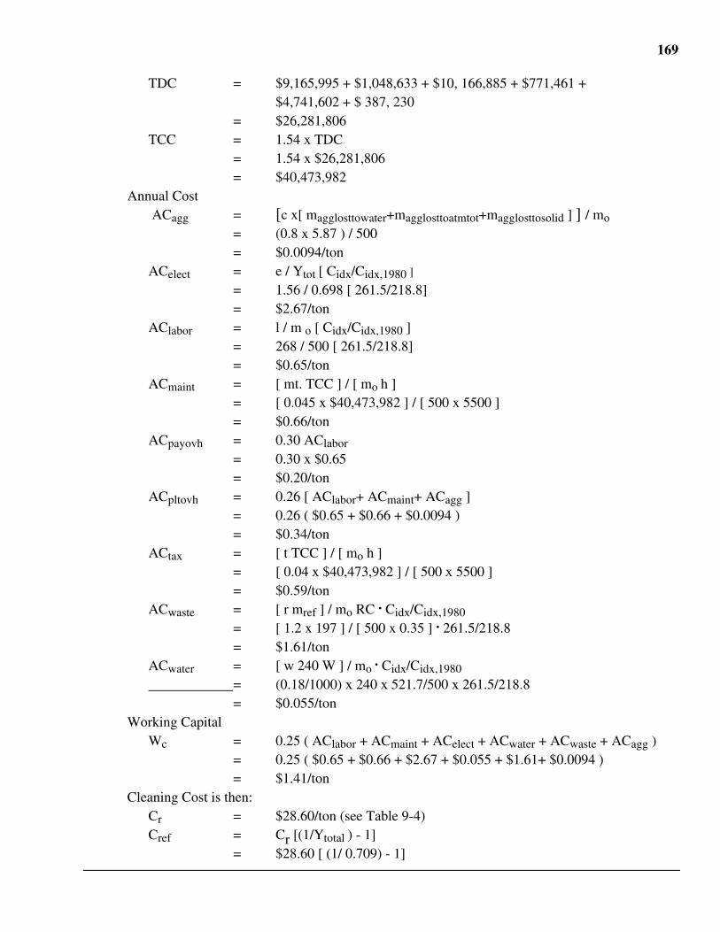
169
TDC = $9,165,995 + $1,048,633 + $10, 166,885 + $771,461 +$4,741,602 + $ 387, 230
= $26,281,806TCC = 1.54 x TDC
= 1.54 x $26,281,806= $40,473,982
Annual Cost ACagg = [c x[ magglosttowater+magglosttoatmtot+magglosttosolid ] ] / mo
= (0.8 x 5.87 ) / 500= $0.0094/ton
ACelect = e / Ytot [ Cidx/Cidx,1980 ]
= 1.56 / 0.698 [ 261.5/218.8]= $2.67/ton
AClabor = l / m o [ Cidx/Cidx,1980 ]= 268 / 500 [ 261.5/218.8]= $0.65/ton
ACmaint = [ mt. TCC ] / [ mo h ]= [ 0.045 x $40,473,982 ] / [ 500 x 5500 ]= $0.66/ton
ACpayovh = 0.30 AClabor
= 0.30 x $0.65= $0.20/ton
ACpltovh = 0.26 [ AClabor+ ACmaint+ ACagg ]= 0.26 ( $0.65 + $0.66 + $0.0094 )= $0.34/ton
ACtax = [ t TCC ] / [ mo h ]= [ 0.04 x $40,473,982 ] / [ 500 x 5500 ]= $0.59/ton
ACwaste = [ r mref ] / mo RC . Cidx/Cidx,1980
= [ 1.2 x 197 ] / [ 500 x 0.35 ] . 261.5/218.8= $1.61/ton
ACwater = [ w 240 W ] / mo . Cidx/Cidx,1980
= (0.18/1000) x 240 x 521.7/500 x 261.5/218.8= $0.055/ton
Working CapitalWc = 0.25 ( AClabor + ACmaint + ACelect + ACwater + ACwaste + ACagg )
= 0.25 ( $0.65 + $0.66 + $2.67 + $0.055 + $1.61+ $0.0094 )= $1.41/ton
Cleaning Cost is then:Cr = $28.60/ton (see Table 9-4)Cref = Cr [(1/Ytotal ) - 1]
= $28.60 [ (1/ 0.709) - 1]
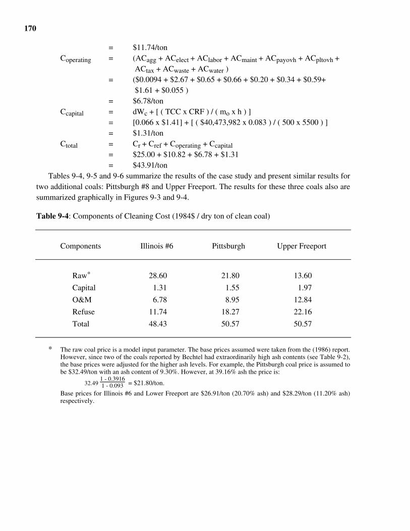
170
= $11.74/tonCoperating = (ACagg + ACelect + AClabor + ACmaint + ACpayovh + ACpltovh +
ACtax + ACwaste + ACwater )= ($0.0094 + $2.67 + $0.65 + $0.66 + $0.20 + $0.34 + $0.59+
$1.61 + $0.055 )= $6.78/ton
Ccapital = dWc + [ ( TCC x CRF ) / ( mo x h ) ]= [0.066 x $1.41] + [ ( $40,473,982 x 0.083 ) / ( 500 x 5500 ) ]= $1.31/ton
Ctotal = Cr + Cref + Coperating + Ccapital
= $25.00 + $10.82 + $6.78 + $1.31= $43.91/ton
Tables 9-4, 9-5 and 9-6 summarize the results of the case study and present similar results fortwo additional coals: Pittsburgh #8 and Upper Freeport. The results for these three coals also aresummarized graphically in Figures 9-3 and 9-4.
Table 9-4: Components of Cleaning Cost (1984$ / dry ton of clean coal)
Components Illinois #6 Pittsburgh Upper Freeport
Raw* 28.60 21.80 13.60
Capital 1.31 1.55 1.97
O&M 6.78 8.95 12.84
Refuse 11.74 18.27 22.16
Total 48.43 50.57 50.57
* The raw coal price is a model input parameter. The base prices assumed were taken from the (1986) report.However, since two of the coals reported by Bechtel had extraordinarily high ash contents (see Table 9-2),the base prices were adjusted for the higher ash levels. For example, the Pittsburgh coal price is assumed tobe $32.49/ton with an ash content of 9.30%. However, at 39.16% ash the price is:
32.49 1 - 0.39161 - 0.093 = $21.80/ton.
Base prices for Illinois #6 and Lower Freeport are $26.91/ton (20.70% ash) and $28.29/ton (11.20% ash)respectively.
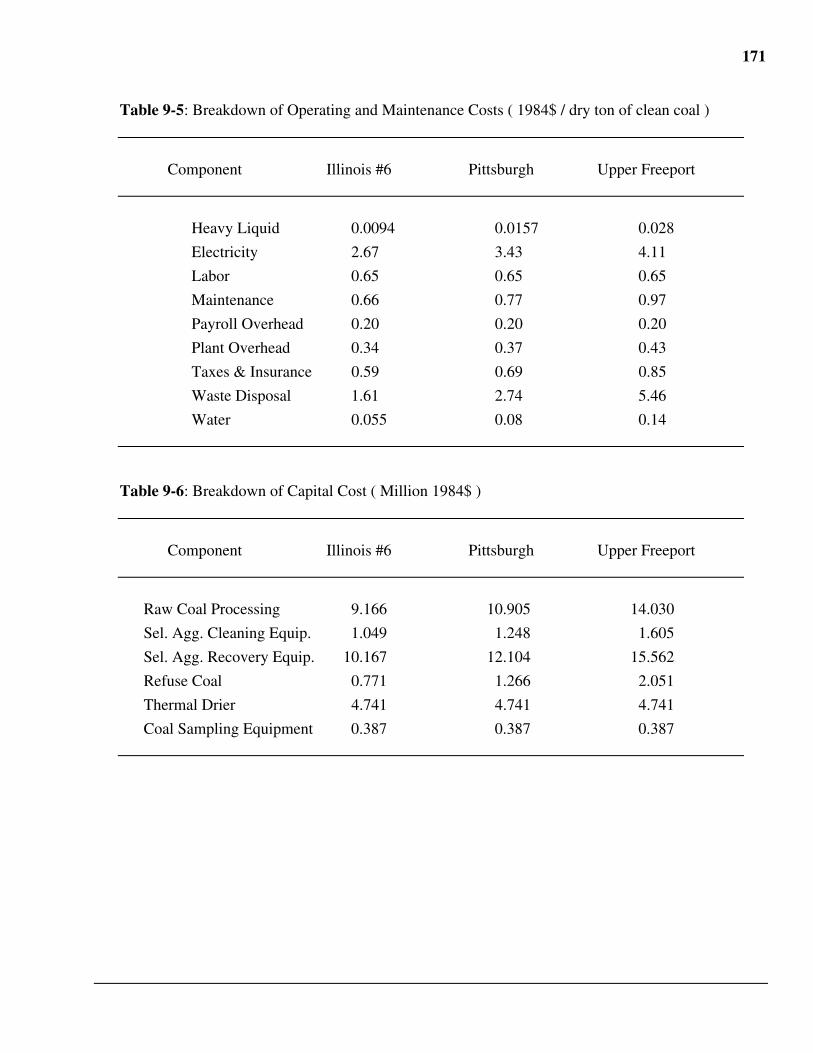
171
Table 9-5: Breakdown of Operating and Maintenance Costs ( 1984$ / dry ton of clean coal )
Component Illinois #6 Pittsburgh Upper Freeport
Heavy Liquid 0.0094 0.0157 0.028
Electricity 2.67 3.43 4.11
Labor 0.65 0.65 0.65
Maintenance 0.66 0.77 0.97
Payroll Overhead 0.20 0.20 0.20
Plant Overhead 0.34 0.37 0.43
Taxes & Insurance 0.59 0.69 0.85
Waste Disposal 1.61 2.74 5.46
Water 0.055 0.08 0.14
Table 9-6: Breakdown of Capital Cost ( Million 1984$ )
Component Illinois #6 Pittsburgh Upper Freeport
Raw Coal Processing 9.166 10.905 14.030
Sel. Agg. Cleaning Equip. 1.049 1.248 1.605
Sel. Agg. Recovery Equip. 10.167 12.104 15.562
Refuse Coal 0.771 1.266 2.051
Thermal Drier 4.741 4.741 4.741
Coal Sampling Equipment 0.387 0.387 0.387
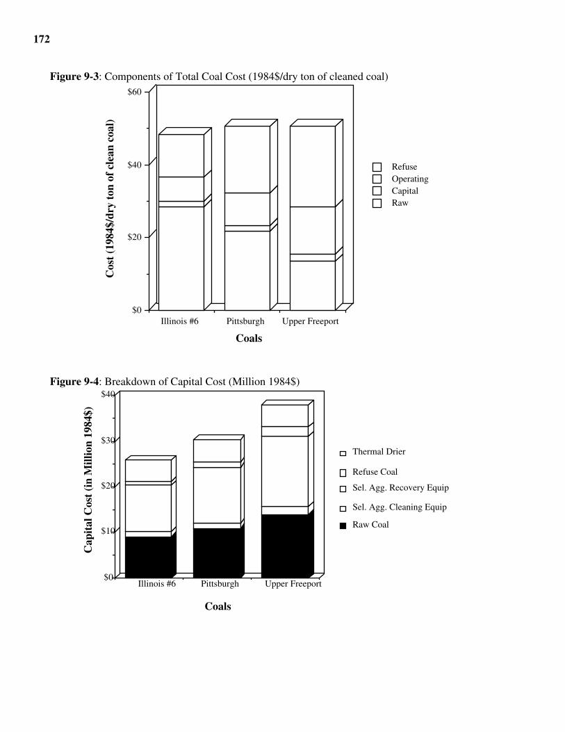
172
Figure 9-3: Components of Total Coal Cost (1984$/dry ton of cleaned coal)
Illinois #6 Pittsburgh Upper Freeport$0
$20
$40
$60
RawCapitalOperatingRefuse
Coals
Cos
t (1
984$
/dry
ton
of
clea
n co
al)
Figure 9-4: Breakdown of Capital Cost (Million 1984$)
Illinois #6 Pittsburgh Upper Freeport$0
$10
$20
$30
$40
Raw Coal
Sel. Agg. Cleaning Equip
Sel. Agg. Recovery Equip
Refuse Coal
Thermal Drier
Coals
Cap
ital
Cos
t (i
n M
illio
n 19
84$)
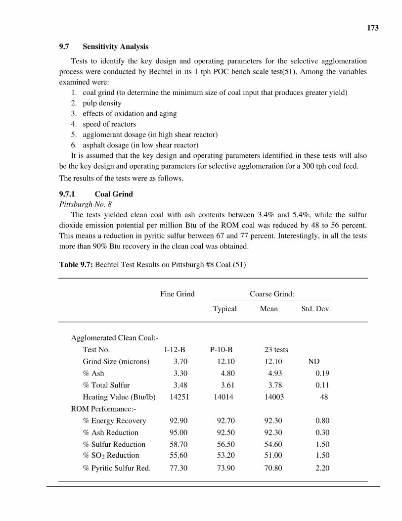
173
9.7 Sensitivity Analysis
Tests to identify the key design and operating parameters for the selective agglomerationprocess were conducted by Bechtel in its 1 tph POC bench scale test(51). Among the variablesexamined were:
1. coal grind (to determine the minimum size of coal input that produces greater yield)2. pulp density3. effects of oxidation and aging4. speed of reactors5. agglomerant dosage (in high shear reactor)6. asphalt dosage (in low shear reactor)It is assumed that the key design and operating parameters identified in these tests will also
be the key design and operating parameters for selective agglomeration for a 300 tph coal feed.
The results of the tests were as follows.
9.7.1 Coal GrindPittsburgh No. 8
The tests yielded clean coal with ash contents between 3.4% and 5.4%, while the sulfurdioxide emission potential per million Btu of the ROM coal was reduced by 48 to 56 percent.This means a reduction in pyritic sulfur between 67 and 77 percent. Interestingly, in all the testsmore than 90% Btu recovery in the clean coal was obtained.
Table 9.7: Bechtel Test Results on Pittsburgh #8 Coal (51)
Fine Grind Coarse Grind:——————————————————————————————————————————————
Typical Mean Std. Dev.
Agglomerated Clean Coal:-
Test No. I-12-B P-10-B 23 tests
Grind Size (microns) 3.70 12.10 12.10 ND
% Ash 3.30 4.80 4.93 0.19
% Total Sulfur 3.48 3.61 3.78 0.11
Heating Value (Btu/lb) 14251 14014 14003 48
ROM Performance:-
% Energy Recovery 92.90 92.70 92.30 0.80
% Ash Reduction 95.00 92.50 92.30 0.30
% Sulfur Reduction 58.70 56.50 54.60 1.50% SO2 Reduction 55.60 53.20 51.00 1.50
% Pyritic Sulfur Red. 77.30 73.90 70.80 2.20
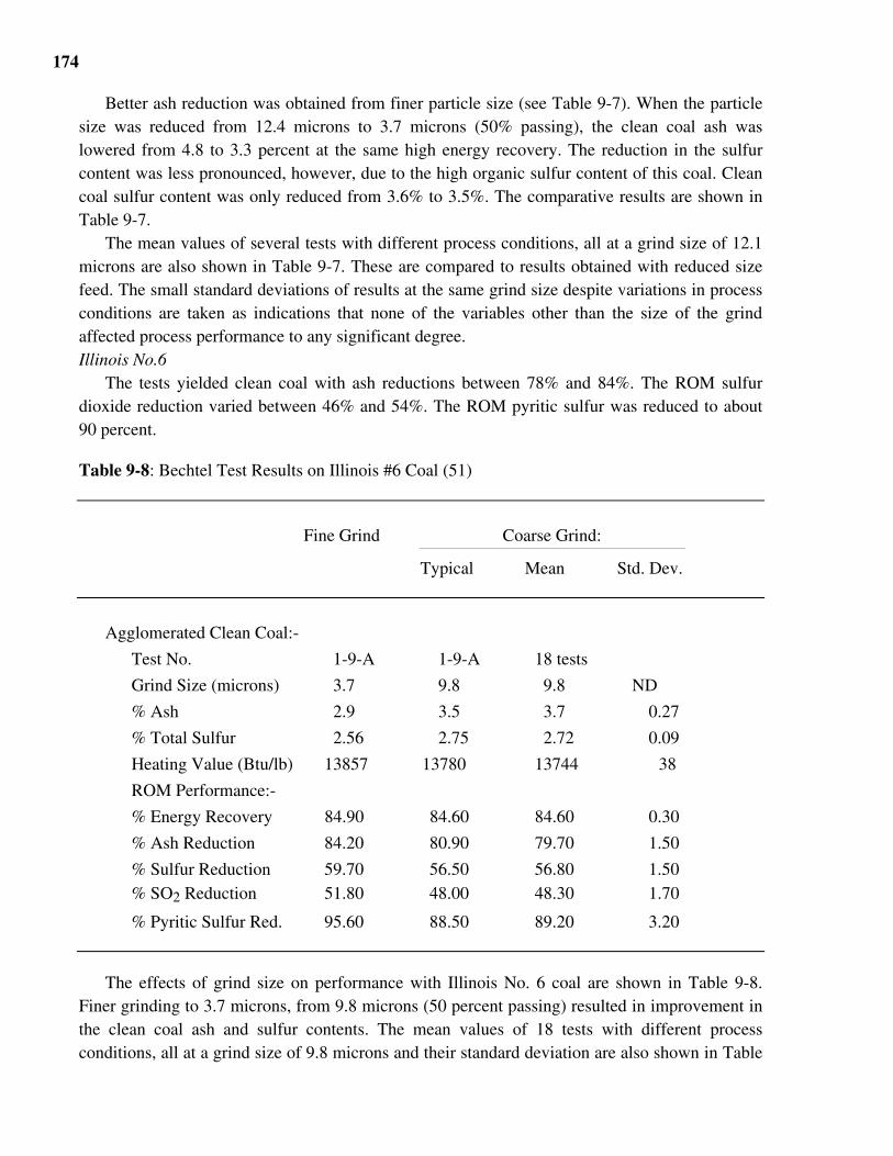
174
Better ash reduction was obtained from finer particle size (see Table 9-7). When the particlesize was reduced from 12.4 microns to 3.7 microns (50% passing), the clean coal ash waslowered from 4.8 to 3.3 percent at the same high energy recovery. The reduction in the sulfurcontent was less pronounced, however, due to the high organic sulfur content of this coal. Cleancoal sulfur content was only reduced from 3.6% to 3.5%. The comparative results are shown inTable 9-7.
The mean values of several tests with different process conditions, all at a grind size of 12.1microns are also shown in Table 9-7. These are compared to results obtained with reduced sizefeed. The small standard deviations of results at the same grind size despite variations in processconditions are taken as indications that none of the variables other than the size of the grindaffected process performance to any significant degree. Illinois No.6
The tests yielded clean coal with ash reductions between 78% and 84%. The ROM sulfurdioxide reduction varied between 46% and 54%. The ROM pyritic sulfur was reduced to about90 percent.
Table 9-8: Bechtel Test Results on Illinois #6 Coal (51)
Fine Grind Coarse Grind:——————————————————————————————————————————————
Typical Mean Std. Dev.
Agglomerated Clean Coal:-
Test No. 1-9-A 1-9-A 18 tests
Grind Size (microns) 3.7 9.8 9.8 ND
% Ash 2.9 3.5 3.7 0.27
% Total Sulfur 2.56 2.75 2.72 0.09
Heating Value (Btu/lb) 13857 13780 13744 38
ROM Performance:-
% Energy Recovery 84.90 84.60 84.60 0.30
% Ash Reduction 84.20 80.90 79.70 1.50
% Sulfur Reduction 59.70 56.50 56.80 1.50% SO2 Reduction 51.80 48.00 48.30 1.70
% Pyritic Sulfur Red. 95.60 88.50 89.20 3.20
The effects of grind size on performance with Illinois No. 6 coal are shown in Table 9-8.Finer grinding to 3.7 microns, from 9.8 microns (50 percent passing) resulted in improvement inthe clean coal ash and sulfur contents. The mean values of 18 tests with different processconditions, all at a grind size of 9.8 microns and their standard deviation are also shown in Table
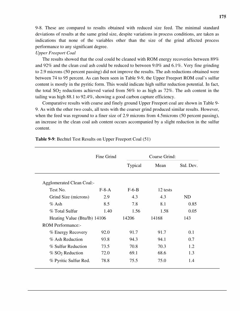
175
9-8. These are compared to results obtained with reduced size feed. The minimal standarddeviations of results at the same grind size, despite variations in process conditions, are taken asindications that none of the variables other than the size of the grind affected processperformance to any significant degree.Upper Freeport Coal
The results showed that the coal could be cleaned with ROM energy recoveries between 89%and 92% and the clean coal ash could be reduced to between 9.0% and 6.1%. Very fine grindingto 2.9 microns (50 percent passing) did not improve the results. The ash reductions obtained werebetween 74 to 95 percent. As can been seen in Table 9-9, the Upper Freeport ROM coal’s sulfurcontent is mostly in the pyritic form. This would indicate high sulfur reduction potential. In fact,the total SO2 reductions achieved varied from 56% to as high as 72%. The ash content in thetailing was high 88.1 to 92.4%, showing a good carbon capture efficiency.
Comparative results with coarse and finely ground Upper Freeport coal are shown in Table 9-9. As with the other two coals, all tests with the coarser grind produced similar results. However,when the feed was reground to a finer size of 2.9 microns from 4.5microns (50 percent passing),an increase in the clean coal ash content occurs accompanied by a slight reduction in the sulfurcontent.
Table 9-9: Bechtel Test Results on Upper Freeport Coal (51)
Fine Grind Coarse Grind:——————————————————————————————————————————————
Typical Mean Std. Dev.
Agglomerated Clean Coal:-
Test No. F-8-A F-6-B 12 tests
Grind Size (microns) 2.9 4.3 4.3 ND
% Ash 8.5 7.8 8.1 0.85
% Total Sulfur 1.40 1.56 1.58 0.05
Heating Value (Btu/lb) 14106 14206 14168 143
ROM Performance:-
% Energy Recovery 92.0 91.7 91.7 0.1
% Ash Reduction 93.8 94.3 94.1 0.7
% Sulfur Reduction 73.5 70.8 70.3 1.2% SO2 Reduction 72.0 69.1 68.6 1.3
% Pyritic Sulfur Red. 78.8 75.5 75.0 1.4
176
9.7.2 Pulp DensityTests were run at 10, 15, 20 and 25 percent solids by weight. At 25 percent solids, the sample
slurries of the fine ground coal all became too strongly non-Newtonian under high shear toagglomerate properly. Illinois No. 6 and Pittsburgh No. 8 samples were run at 20 percent solids,where their fluid mechanical properties were marginal. The results indicated that Pittsburgh No.8 performed marginally worse at 20 percent solids, but that Illinois No. 6 showed no significantchange. No detectable change in performance was seen for any of the samples agglomerated at10 percent as compared to 15 percent. These results led to the selection of a solids concentrationof 15 percent in the nominal selective agglomeration process design.
9.7.3 Agglomerant DosageIn a high shear reactor (where the agglomerate is added to the slurry), the approximate speed
is 12,000 rpm. Given an adequate quantity to sustain agglomeration, the agglomerant dosageaffects only the size of the agglomerates and not the product quality or energy recovery.Agglomerant dosages (by weight percent of dry coal feed) of 25% or up are recommended forPittsburgh No.8 and Illinois No.6 and agglomerant dosages 35% or up for Upper Freeport.
9.7.4 Asphalt DosageIn low shear reactor (where asphalt binder is added to the mixture of agglomerate and slurry),
the approximate speed is 6,000 rpm. Asphalt dosage affects product size and strength.Agglomerates of adequate strength are required to avoid carbon losses during product screening.Asphalt dosages (by weight percent of dry coal feed) of 4% or up are recommended forPittsburgh No.8, Illinois No.6 and Upper Freeport. Since the cost of adding the asphalt to theprocess is marginal compared to other costs, we dropped it in calculating the cost of the entirecoal cleaning process.
9.7.5 Effects on EconomicsThe cleaning cost (excluding the raw coal cost) for Illinois #6 coal for the two different grind
sizes of coal input noted earlier was investigated. The results of this sensitivity analysis suggestthat as 9.8 microns coal was ground to 3.7 microns, the sulfur content of cleaned coal wasreduced by 5%. Still, the cleaning cost increased by $1 per dry ton of cleaned coal (Figure 9-5).
The cleaning cost for Illinois #6 coal for the two different solids concentrations (pulp density)was also investigated. The results of this sensitivity analysis suggested that an increase of 5%solid concentration could lead to about a 0.3% increase in sulfur reduction and an additional$0.30 increase in clean cost per dry ton of cleaned coal (Figure 9-6). The results support theselection of 15% solid concentration in the selective agglomeration process.
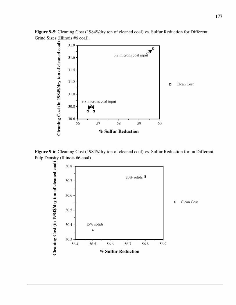
177
Figure 9-5: Cleaning Cost (1984$/dry ton of cleaned coal) vs. Sulfur Reduction for DifferentGrind Sizes (Illinois #6 coal).
605958575630.6
30.8
31.0
31.2
31.4
31.6
31.8
Clean Cost
% Sulfur Reduction
Cle
anin
g C
ost
(in
1984
$/dr
y to
n of
cle
aned
coa
l)
9.8 microns coal input
3.7 microns coal input
Figure 9-6: Cleaning Cost (1984$/dry ton of cleaned coal) vs. Sulfur Reduction for on DifferentPulp Density (Illinois #6 coal).
56.956.856.756.656.556.430.3
30.4
30.5
30.6
30.7
30.8
Clean Cost
% Sulfur Reduction
Cle
anin
g C
ost
(in
1984
$/dr
y to
n of
cle
aned
coa
l)
15% solids
20% solids
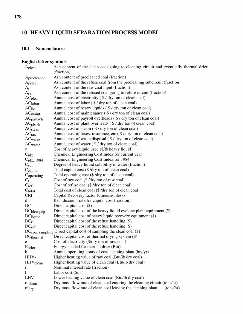
178
10 HEAVY LIQUID SEPARATION PROCESS MODEL
10.1 Nomenclature
English letter symbolsAclean Ash content of the clean coal going to cleaning circuit and eventually thermal drier
(fraction)Aprecleaned Ash content of precleaned coal (fraction)Apreref Ash content of the refuse coal from the precleaning subcircuit (fraction)Ar Ash content of the raw coal input (fraction)Aref Ash content of the refused coal going to refuse circuit (fraction)ACelect Annual cost of electricity ( $ / dry ton of clean coal)AClabor Annual cost of labor ( $ / dry ton of clean coal)ACliq Annual cost of heavy liquids ( $ / dry ton of clean coal)ACmaint Annual cost of maintenance ( $ / dry ton of clean coal)ACpayovh Annual cost of payroll overheads ( $ / dry ton of clean coal)ACplovh Annual cost of plant overheads ( $ / dry ton of clean coal)ACsteam Annual cost of steam ( $ / dry ton of clean coal)ACtax Annual cost of taxes, insurance, etc ( $ / dry ton of clean coal)ACwaste Annual cost of waste disposal ( $ / dry ton of clean coal)ACwater Annual cost of water ( $ / dry ton of clean coal)c Cost of heavy liquid used ($/lb heavy liquid)Cidx Chemical Engineering Cost Index for current yearCidx, 1984 Chemical Engineering Cost Index for 1984Csol Degree of heavy liquid solubility in water (fraction)Ccapital Total capital cost ($ /dry ton of clean coal)Coperating Total operating cost ($ /dry ton of clean coal)Cr Cost of raw coal ($ /dry ton of raw coal)Cref Cost of refuse coal ($ /dry ton of clean coal)Ctotal Total cost of clean coal ($ /dry ton of clean coal)CRF Capital Recovery factor (dimensionless)d Real discount rate for capital cost (fraction)DC Direct capital cost ($)DChlcequip Direct capital cost of the heavy liquid cyclone plant equipment ($)DCliqrec Direct capital cost of heavy liquid recovery equipment ($)DCr Direct capital cost of the refuse handling ($)DCref Direct capital cost of the refuse handling ($)DCcoal sampling Direct capital cost of sampling the clean coal ($)DCthermal Direct capital cost of thermal drying system ($)e Cost of electricity ($/dry ton of raw coal)Edrier Energy needed for thermal drier (Btu)h Annual operating hours of coal cleaning plant (hrs/yr)HHVr Higher heating value of raw coal (Btu/lb dry coal)HHVclean Higher heating value of clean coal (Btu/lb dry coal)i Nominal interest rate (fraction)l Labor cost ($/hr)LHV Lower heating value of clean coal (Btu/lb dry coal)mclean Dry mass flow rate of clean coal entering the cleaning circuit (tons/hr)mdry Dry mass flow rate of clean coal leaving the cleaning plant (tons/hr)
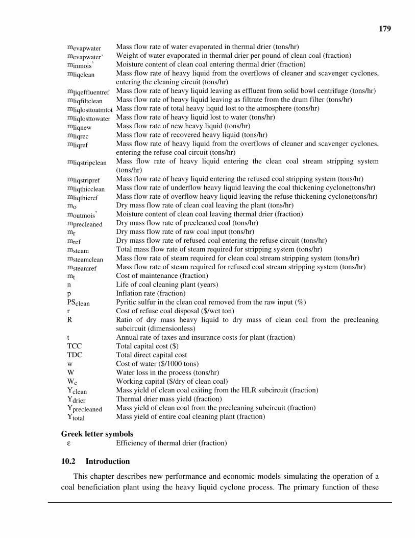
179
mevapwater Mass flow rate of water evaporated in thermal drier (tons/hr)mevapwater’ Weight of water evaporated in thermal drier per pound of clean coal (fraction)minmois’ Moisture content of clean coal entering thermal drier (fraction)mliqclean Mass flow rate of heavy liquid from the overflows of cleaner and scavenger cyclones,
entering the cleaning circuit (tons/hr)mliqeffluentref Mass flow rate of heavy liquid leaving as effluent from solid bowl centrifuge (tons/hr)mliqfiltclean Mass flow rate of heavy liquid leaving as filtrate from the drum filter (tons/hr)mliqlosttoatmtot Mass flow rate of total heavy liquid lost to the atmosphere (tons/hr)mliqlosttowater Mass flow rate of heavy liquid lost to water (tons/hr)mliqnew Mass flow rate of new heavy liquid (tons/hr)mliqrec Mass flow rate of recovered heavy liquid (tons/hr)mliqref Mass flow rate of heavy liquid from the overflows of cleaner and scavenger cyclones,
entering the refuse coal circuit (tons/hr)mliqstripclean Mass flow rate of heavy liquid entering the clean coal stream stripping system
(tons/hr)mliqstripref Mass flow rate of heavy liquid entering the refused coal stripping system (tons/hr)mliqthicclean Mass flow rate of underflow heavy liquid leaving the coal thickening cyclone(tons/hr)mliqthicref Mass flow rate of overflow heavy liquid leaving the refuse thickening cyclone(tons/hr)mo Dry mass flow rate of clean coal leaving the plant (tons/hr)moutmois’ Moisture content of clean coal leaving thermal drier (fraction)mprecleaned Dry mass flow rate of precleaned coal (tons/hr)mr Dry mass flow rate of raw coal input (tons/hr)mref Dry mass flow rate of refused coal entering the refuse circuit (tons/hr)msteam Total mass flow rate of steam required for stripping system (tons/hr)msteamclean Mass flow rate of steam required for clean coal stream stripping system (tons/hr)msteamref Mass flow rate of steam required for refused coal stream stripping system (tons/hr)mt Cost of maintenance (fraction)n Life of coal cleaning plant (years)p Inflation rate (fraction)PSclean Pyritic sulfur in the clean coal removed from the raw input (%)r Cost of refuse coal disposal ($/wet ton)R Ratio of dry mass heavy liquid to dry mass of clean coal from the precleaning
subcircuit (dimensionless)t Annual rate of taxes and insurance costs for plant (fraction)TCC Total capital cost ($)TDC Total direct capital costw Cost of water ($/1000 tons)W Water loss in the process (tons/hr)Wc Working capital ($/dry of clean coal)Yclean Mass yield of clean coal exiting from the HLR subcircuit (fraction)Ydrier Thermal drier mass yield (fraction)Yprecleaned Mass yield of clean coal from the precleaning subcircuit (fraction)Ytotal Mass yield of entire coal cleaning plant (fraction)
Greek letter symbolsε Efficiency of thermal drier (fraction)
10.2 Introduction
This chapter describes new performance and economic models simulating the operation of acoal beneficiation plant using the heavy liquid cyclone process. The primary function of these
180
models is to estimate the cost and ability of the process to remove pyritic sulfur and ash contentto help meet power plant emission standards. This report presents a brief overview of heavyliquid cyclones, a description of the economic algorithms and an assessment of this process’ability to reduce sulfur dioxide emissions of coal fired power plants. Models are adopted frombench-scale test on a one ton per hour (tph) Proof-of-Concept (POC) units performed by ProcessTechnology Institute (PTI)21 (53). An assessment of capital investment and operating costs for aheavy liquid cyclone process for a plant size of 300 tph proposed by Burns and Roe ServicesCorporation (52) is adopted in developing the economic model.
The heavy liquid cyclone process uses the differences in specific gravity (s.g.) between thecoal and liberated pyrites to achieve separation. In this process, coal (s.g. ~ 1.30) is mixed with aheavy liquid of specific gravity between 1.33 to 1.60 and passed through a cyclone. The highcentrifugal forces experienced by the coal and the liberated pyrites in the heavy liquid promoteseparation by moving the lighter coal particles to the center and the heavier pyrites particles tothe wall of the cyclone. The clean coal reports as overflow and the heavy impurities asunderflow.
The process design is based on 2” to 4” diameter cyclones. Because of the small throughputcapacity of these cyclones, a large number of cyclones is required. Effective distribution of thefeed material to the cyclones is a challenging problem. Because of these uncertainties in theperformance of cyclones, the operating cost of cyclones is a cost-sensitive area. Another cost-sensitive area is recovery of the heavy liquid.
10.3 Process Description
A conceptual flow scheme for an HLC process is shown in Figure 10-1 and 10-2. The HLCprocess comprises of two subcircuits: heavy liquid cyclone subcircuit and heavy liquid recoverysubcircuit. Two other subcircuits also contributed to the HLC process discussed here. They arethe precleaning subcircuit and the comminution subcircuit.
10.3.1 Precleaning SubcircuitThe objective of the precleaning circuit (flowsheet not shown) was to remove the out-of-seam
dilution rock that is collected during the normal course of mining operations. Because most ofthis rock is coarse, it is advantageous to remove the rock prior to grinding to avoid energyintensive grinding process and fine particle separation difficulties. Heavy medium cyclone circuitwould be used to remove the most coarse rock and maintain high thermal recovery.
In this subcircuit, the ROM feed was crushed to 3/8” and screened at 8 mesh. The 3/8” x 8mesh material was subjected to cleaning in the heavy medium cyclone while the -8 meshmaterial was saved for recombination with the precleaned +8 mesh material.
The 3/8” x 8 mesh coal was fed continuously into a sump where it was mixed with the water.A 5” kreb cyclone was used to make separation. The clean coal and refuse products werecollected off the drain and rinse screens into 55 gallon barrels. These 55 gallon barrels wereremoved to storage alongside the -8 mesh material. The +8 mesh and the -8 mesh material were
21 There are four other groups involved in the project: Michigan Technological University (MTU); Bateman
Engineer, Inc (BE); Norton, Hambleton Engineering Inc. (NHE); and, American Electric Power (AEP).
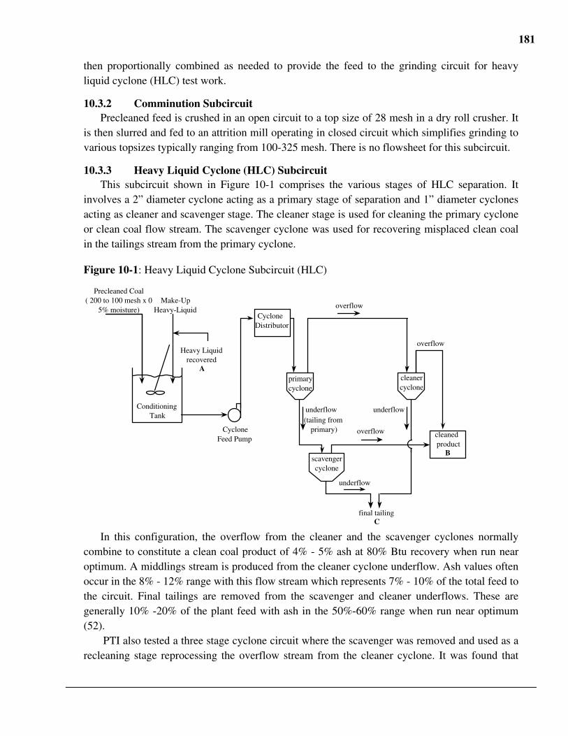
181
then proportionally combined as needed to provide the feed to the grinding circuit for heavyliquid cyclone (HLC) test work.
10.3.2 Comminution SubcircuitPrecleaned feed is crushed in an open circuit to a top size of 28 mesh in a dry roll crusher. It
is then slurred and fed to an attrition mill operating in closed circuit which simplifies grinding tovarious topsizes typically ranging from 100-325 mesh. There is no flowsheet for this subcircuit.
10.3.3 Heavy Liquid Cyclone (HLC) SubcircuitThis subcircuit shown in Figure 10-1 comprises the various stages of HLC separation. It
involves a 2” diameter cyclone acting as a primary stage of separation and 1” diameter cyclonesacting as cleaner and scavenger stage. The cleaner stage is used for cleaning the primary cycloneor clean coal flow stream. The scavenger cyclone was used for recovering misplaced clean coalin the tailings stream from the primary cyclone.
Figure 10-1: Heavy Liquid Cyclone Subcircuit (HLC)
overflow
primary cyclone
(tailing from primary)
underflow
overflow
overflow
scavenger cyclone
cleaned product
B
cleaner cyclone
final tailing C
Precleaned Coal
( 200 to 100 mesh x 0 5% moisture)
Make-Up Heavy-Liquid
Cyclone Distributor
Heavy Liquid recovered
A
Cyclone Feed Pump
Conditioning Tank
underflow
underflow
In this configuration, the overflow from the cleaner and the scavenger cyclones normallycombine to constitute a clean coal product of 4% - 5% ash at 80% Btu recovery when run nearoptimum. A middlings stream is produced from the cleaner cyclone underflow. Ash values oftenoccur in the 8% - 12% range with this flow stream which represents 7% - 10% of the total feed tothe circuit. Final tailings are removed from the scavenger and cleaner underflows. These aregenerally 10% -20% of the plant feed with ash in the 50%-60% range when run near optimum(52).
PTI also tested a three stage cyclone circuit where the scavenger was removed and used as arecleaning stage reprocessing the overflow stream from the cleaner cyclone. It was found that
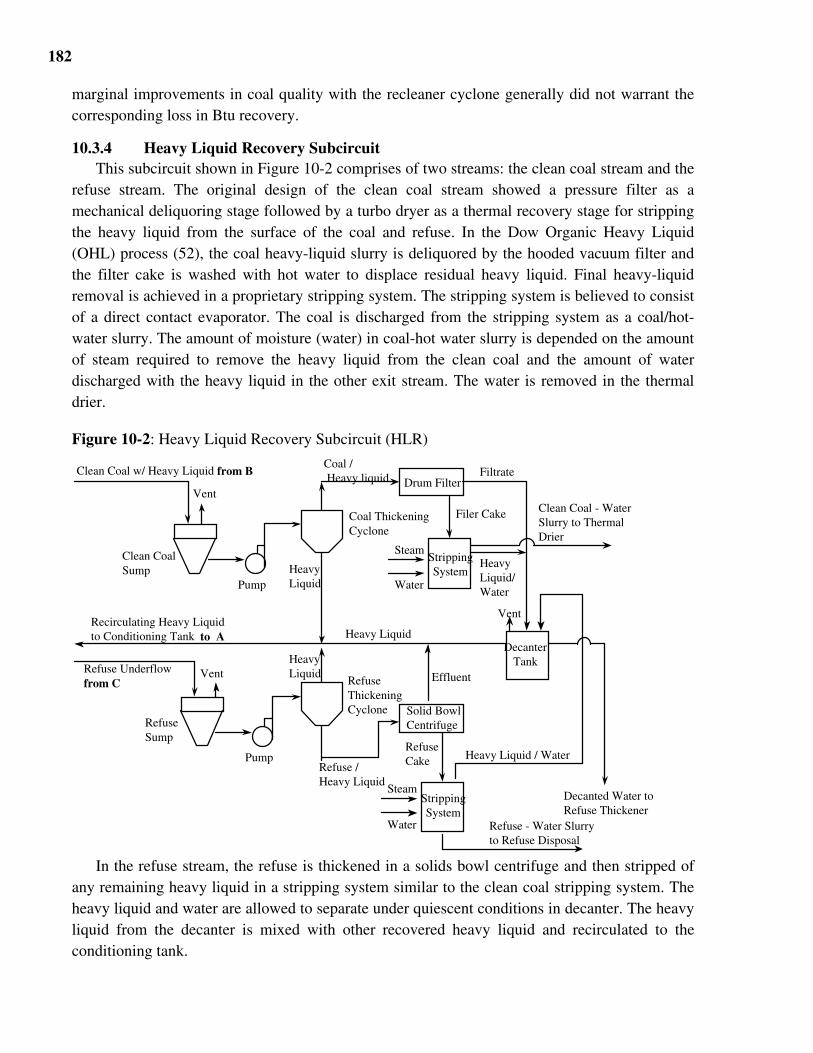
182
marginal improvements in coal quality with the recleaner cyclone generally did not warrant thecorresponding loss in Btu recovery.
10.3.4 Heavy Liquid Recovery SubcircuitThis subcircuit shown in Figure 10-2 comprises of two streams: the clean coal stream and the
refuse stream. The original design of the clean coal stream showed a pressure filter as amechanical deliquoring stage followed by a turbo dryer as a thermal recovery stage for strippingthe heavy liquid from the surface of the coal and refuse. In the Dow Organic Heavy Liquid(OHL) process (52), the coal heavy-liquid slurry is deliquored by the hooded vacuum filter andthe filter cake is washed with hot water to displace residual heavy liquid. Final heavy-liquidremoval is achieved in a proprietary stripping system. The stripping system is believed to consistof a direct contact evaporator. The coal is discharged from the stripping system as a coal/hot-water slurry. The amount of moisture (water) in coal-hot water slurry is depended on the amountof steam required to remove the heavy liquid from the clean coal and the amount of waterdischarged with the heavy liquid in the other exit stream. The water is removed in the thermaldrier.
Figure 10-2: Heavy Liquid Recovery Subcircuit (HLR) Clean Coal w/ Heavy Liquid from B
Pump
Vent
Pump
Vent
Clean Coal Sump
Coal Thickening Cyclone
Coal / Heavy liquid Drum Filter
Steam
Water
Filer Cake
Filtrate
Heavy Liquid/ Water
Heavy Liquid
Decanter Tank
VentRecirculating Heavy Liquid to Conditioning Tank to A
Refuse Underflow from C Refuse
Thickening Cyclone
Refuse / Heavy Liquid
Heavy Liquid
Heavy Liquid
Solid Bowl Centrifuge
Effluent
Refuse Cake
Steam
Water
Stripping System
Refuse - Water Slurry to Refuse Disposal
Heavy Liquid / Water
Refuse Sump
Stripping System
Clean Coal - Water Slurry to Thermal Drier
Decanted Water to Refuse Thickener
In the refuse stream, the refuse is thickened in a solids bowl centrifuge and then stripped ofany remaining heavy liquid in a stripping system similar to the clean coal stripping system. Theheavy liquid and water are allowed to separate under quiescent conditions in decanter. The heavyliquid from the decanter is mixed with other recovered heavy liquid and recirculated to theconditioning tank.
183
It is recommended that when designing the HLC and HLR subcircuits, all the equipment inthe circuit be vented to a collection system to minimize the heavy liquid losses. All theequipment should be air tight. The piping should be designed to prevent losses of the heavyliquid vapors. Basides the losses to the atmosphere, the heavy liquid also lost to the water. Thedetailed calculation of heavy liquid losses are discussed later in illustrative results.
10.4 Performance Model
The algorithm for the determining the higher heating value is as follows:
HHVclean = HHVr [ 1 - Aclean / 1 - Ar ]
Estimates of plant operating and capital costs typically are scaled to various mass flow rateswithin the coal cleaning plant. Those developed below are the rate of raw coal and heavy liquidinto the plant, the rate of dry and wet refuse coal out of the plant, the rate of heavy liquidrecovered and lost from the plant, the rate steam and water required for stripping the heavy liquidand the rate of water evaporated in the thermal drier.
In approaching the performance models developed, we will look at one subcircuit at a time.
10.4.1 Precleaning SubcircuitThe yield of the clean coal going into the Communition subcircuit is calculated as follows:
Yprecleaned = [ Apreref - Ar ] / [ Apreref - Aprecleaned ] (10.1)
10.4.2 Communition SubcircuitWe assume the grinding process does not significantly affect the percentage yield of
precleaned coal. Yprecleaned obtained from Equation (10.1) remains as the ground precleanedcoal enters the HLC subcircuit.
10.4.3 HLC SubcircuitThe amount of heavy liquid needed for this process related to the specific gravity of the coal
and the specific gravity of the heavy liquid. The ratio of mass of heavy liquid to the dry mass ofprecleaned coal is denoted by R, or
mliq = Rm precleaned
The value of R is determined from experiments.The yield of the clean coal going into the HLR subcircuit is calculated as follows:
Yclean = [ Aref - Aprecleaned ] / [ Aref - Aclean ]
10.4.4 HLR SubcircuitAs was mentioned earlier, we have divided this subcircuit into two streams -- the clean coal
and refuse coal streams. We will look at the clean coal stream first.Clean Coal Stream
The mass flow rate of the heavy liquid entering this stream, mliqclean, is the sum of the massflow rate of the underflow of the coal thickening cyclone, mliqthicclean and the heavy liquidexiting from the drum filter ( mliqfiltclean + mliqstripclean ):
184
mliqclean = mliqthicclean + mliqfiltclean + mliqstripclean
The amount of stream needed in clean coal stripping system was
msteamclean = 0.149 mliqstripclean (10.2)
Refuse Coal StreamThe approach in developing the following equations for the refuse coal stream is similar to
the one discussed in the clean coal stream. The mass flow rate of the heavy liquid entering thisstream, mliqref, is the sum of the mass flow rate of the overflow of the refuse thickening cyclone,mliqthicref and the heavy liquid exiting from the solid bowl centrifuge ( mliqeffluentref andmliqstripref ):
mliqref = mliqthicref + mliqeffluentref + mliqstripref
The amount of steam and cooling water needed in refuse stripping system is calculated byequations follows:
msteamref = 0.149 mliqstripref (10.3)
Combining equations (10.2) and (10.3), the total steam consumption is therefore
msteam = msteamclean + msteamref = 0.149 (mliqstripclean + mliqstripref)
By tabulating the experimental data
mliqstripclean + mliqstripref = 0.436 mliq
Therefore,
msteam = 0.149 x 0.436 x mliq
= 65.0 x 10⁻³ mliq
Not all the heavy liquid will be recovered. Depending on the degree of solubility of heavyliquid in water, some will be lost to the water. The amount of heavy liquid that is lost to thewater is estimated to be
mliqlosttowater = Csol x W
where W is the total water loss in the processBesides the losses of the heavy liquid to the water in both stripping system, some heavy
liquid is also lost to the atmosphere. To find the heavy liquid that is lost to the atmosphere, wehave to consider the entire components of HLC and HLR subcircuits. The formula obtained isshown below:
mliqlosttoatmtot = 3.5 x 10⁻⁴ mprecleaned
Hence, the recovered heavy liquid (methylene chloride) from this stream is
(mliqrec) = mliqclean + mliqref - mliqlosttowater - mliqlosttoatmtot (10.4)
Since the sum of mliqclean + mliqref is also the sum of mliqnew + mliqrec, equation (10.4) isreduced to
mliqrec = ( mliqnew + mliqrec ) - mliqlosttowater - mliqlosttoatmtot
or
185
mliqnew = mliqlosttowater + mliqlosttoatmtot
10.4.5 Thermal Drier SubcircuitNormally, it is necessary to thermally dry the fine sizes of coal-hot water slurry. It is assumed
that product coal is used to fire the thermal drier, thus reducing the overall plant yield (thissubcircuit is not shown in the flowsheet). It is also assumed that drying alters only the coalmoisture content, with all the other coal properties (measured on a dry basis) remain the same.Since the moisture content of coal entering and leaving the thermal drier is specified, the weightof the water evaporated per pound of precleaned coal into the thermal drier is
mevapwater’ = [minmois’ - moutmois’] / [ ( 1 - minmois’ ) ( 1 - moutmois’ ) ]
The amount of energy needed to evaporate this water is
Ed = 1020 mevapwater’ / ε
The lower heating value can be approximated by
LHV = 0.96 HHVclean - [ 1020 moutmois’ / ( 1 - moutmois’ ) ]
Therefore, the drier yield and total plant yield are given by
Ydrier = 1 - Ed / LHV
and
Ytotal = YprecleanedYcleanYdrier
The weight of water evaporated is
mevapwater = mevapwater’ [ mo / Ydrier ]
Once the drier is determined, the dry mass flow rates for the raw coal stream, refuse streamand drier stream can be calculated by the following equations:
mr = mo / Ytotal
mprecleaned = mo x Yprecleaned
mdry = mo / Ydrier
mref = mo - mdry
The water loss in the coal cleaning plant is
W =mdry [ ( 1 / ( 1 - minmois’)) -1] + mref [ ( 1 / RC ) - 1 )
10.5 Economic Model
The total cost in dollars per ton of dry clean coal can be divided into four separate costscategories.
• cost of raw coal• cost of rejected coal• annual operating and maintenance costs• annualized capital costs
186
The cost of raw coal is an input parameter. The cost of the refuse cost is a function of theplant yield and can be calculated from
Cref = Cr [(1/Ytotal ) - 1] (10.5)
10.5.1 Capital CostThe capital cost is divided into five different sections: raw coal handling, heavy liquid
cyclone equipment, heavy liquid handling, refuse handling and thermal driers (if needed). Thecapital costs related to clean coal storage is included in the raw coal cost, since the coal cleaningequipment is assumed to be at the mine site. This includes the cost for conveyors, storage andloading equipment. The raw coal cost also includes the related capital cost from the precleaningprocess. This includes heavy mediums cyclones, sieve bends, coal screens and coal centrifuges.The cost of handling the refuse from the precleaning process is combined with the cost ofhandling the refuse from the HLR subcircuit. This direct capital cost for refuse handling includesrefuse sump, explosion proof pump, refuse thickening cyclone, centrifuges and refuse strippingsystem. The direct capital cost is determined by these equations:
DCr = $ 22, 524 mr0.7 x [Cidx / Cidx,1984] (10.6)
DChlcequip = $22, 528 mprecleaned0.7 x [Cidx / Cidx,1984] (10.7)
DCliqrec = $ 30,643 (mliqnew + mligrec)0.7 x [Cidx / Cidx,1984]
= $ 30,643 x (Rmr)0.7 x [Cidx / Cidx,1984] (10.8)
DCref = $33, 514 mref0.7 x [Cidx / Cidx,1984] (10.9)
DCdrier = $153, 000 mevapwater0.7 x [Cidx / Cidx,1984] (10.10)
DCcoalsampling = $324,000 x [Cidx / Cidx,1980] (10.11)
The direct capital cost for the HLC subcircuit equipment covers the cost for the 20,000 galloncast iron conditioning tank, agitator of 200 horsepower, cyclone feed pump and three set ofcyclones -- primary, cleaner and scavenger. Clean coal sump, pump, coal thickening cyclone,drum filter and clean coal stripping system are included in DCclean.
The total direct capital cost is found by adding Equation (10.6) through (10.11)
TDC = DCr + DChlcequip + DCliqrec + DCref + DCdrier - DCcoalsampling
The indirect capital and contingencies costs are estimated to be 56% of the direct capital cost.Therefore, the total capital cost, which is depreciated over the life of the plant is
TCC = 1.56 TDC
The total capital cost is annualized as follows:
d = [ ( 1 + i ) / ( 1 + p ) - 1 ]
where i is the interest rate and p is the inflation rate. Therefore, capital recover factor is
CRF = d / [ 1 - ( 1 + d )-n ]
187
Working capital is estimated to be 25% of the labor, maintenance, electricity, water, wastedisposal and heavy liquid costs as in the conventional plant model described in Chapter 2.
Wc = 0.25 ( AClabor + ACmaint + ACelect + ACwater + ACwaste + ACliq + ACsteam)
As in Chapter 2, the capital cost in ($ per dry ton of clean coal) is
Ccapital = [ dWc + [ ( TCC x CRF ) / ( mo x h ) ] ] (10.12)
10.5.2 Operating and Maintenance CostThe annual operating and maintenance costs comprise several cost elements, including labor,
maintenance, raw material and waste disposal costs, also taxes, insurance and generaladministrative overhead. The operating and maintenance cost is broken down into ninecomponents.
• heavy liquid• electricity• labor• maintenance• payroll overhead• taxes and insurance• waste disposal• water• steamTable 10-1 shows the cost factors for various components. The total annual cost of heavy
liquid in $/ton of clean coal is estimated to be
ACliq = [ c x mliqnew] ] / mo The cost of labor is estimated to be dependent of plant size. Maintenance costs, taxes and
insurance are estimated to be proportional to the total capital cost of the plant. The cost ofelectricity is linked to the mass flow rate of the coal entering the plant, while the cost of wastedisposal is proportional to the quantity of coal rejected. The cost for water is proportional to theamount of water in the clean coal and refuse streams. Overhead costs are based on labor,maintenance and heavy liquid costs. The equations for these costs are
ACelect = e / Ytot x [Cidx / Cidx,1980]
AClabor = l / m o x [Cidx / Cidx,1980]
ACmaint = [ mt. TCC ] / [ mo h ]
ACpayovh = 0.30 AClabor
ACpltovh = 0.26 [ AClabor+ ACmaint+ ACliq ]
ACtax = [ t TCC ] / [ mo h ]
ACwaste = [ r mref ] / mo RC x [Cidx / Cidx,1980]
ACwater = [ w 240 W ] / mo x [Cidx / Cidx,1980]
188
ACsteam = s x msteam / mo x [Cidx / Cidx,1980]
where e, l, m, r, s and w are taken from Table 10-1. Adding the above equations and converting
to a base year yields:
Coperating = Cidx (ACliq + ACelect + AClabor + ACmaint + ACpayovh + ACpltovh
+ ACtax+ ACwaste + ACwater + ACsteam (10.13)
The total cost for clean coal is found by adding Equations (10.5), (10.12), (10.13) and the rawcoal cost
Ctotal = Craw + Cref + Coperating + Ccapital
Table 10-1: Operating Cost Factors (1980 $)
Variable Cost Elements Symbol Definition Value
Electricity e ($/raw ton) 1.560
Labor l ($/hr) 268.000
Maintenance mt (fraction) 0.045
Refuse Disposal r ($/wet ton) 1.200
Taxes t (fraction) 0.040
Water w ($/1000 gallon) 0.180
Heavy Liquid c ($/lb) 0.800
10.6 Illustrative Results
Experimental HLC process done by PTI on Pittsburgh coal and Illinois No.6 coal is shown in
Table 10-2. In this process the heavy liquid used is methylene chloride. Methylene chloride is
chosen over Freon-113 (another heavy liquid considered) since the lower specific gravity of
methylene chloride (s.g. 1.33) will give better product quality than the process based on Freon-
113 (s.g. 1.57). The relevant properties of methylene chloride and Freon-113 are listed in Table
10-3.
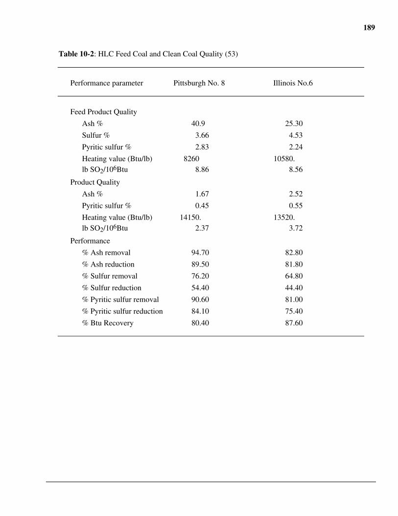
189
Table 10-2: HLC Feed Coal and Clean Coal Quality (53)
Performance parameter Pittsburgh No. 8 Illinois No.6
Feed Product Quality
Ash % 40.9 25.30
Sulfur % 3.66 4.53
Pyritic sulfur % 2.83 2.24
Heating value (Btu/lb) 8260 10580.lb SO2/106Btu 8.86 8.56
Product Quality
Ash % 1.67 2.52
Pyritic sulfur % 0.45 0.55
Heating value (Btu/lb) 14150. 13520.lb SO2/106Btu 2.37 3.72
Performance
% Ash removal 94.70 82.80
% Ash reduction 89.50 81.80
% Sulfur removal 76.20 64.80
% Sulfur reduction 54.40 44.40
% Pyritic sulfur removal 90.60 81.00
% Pyritic sulfur reduction 84.10 75.40
% Btu Recovery 80.40 87.60
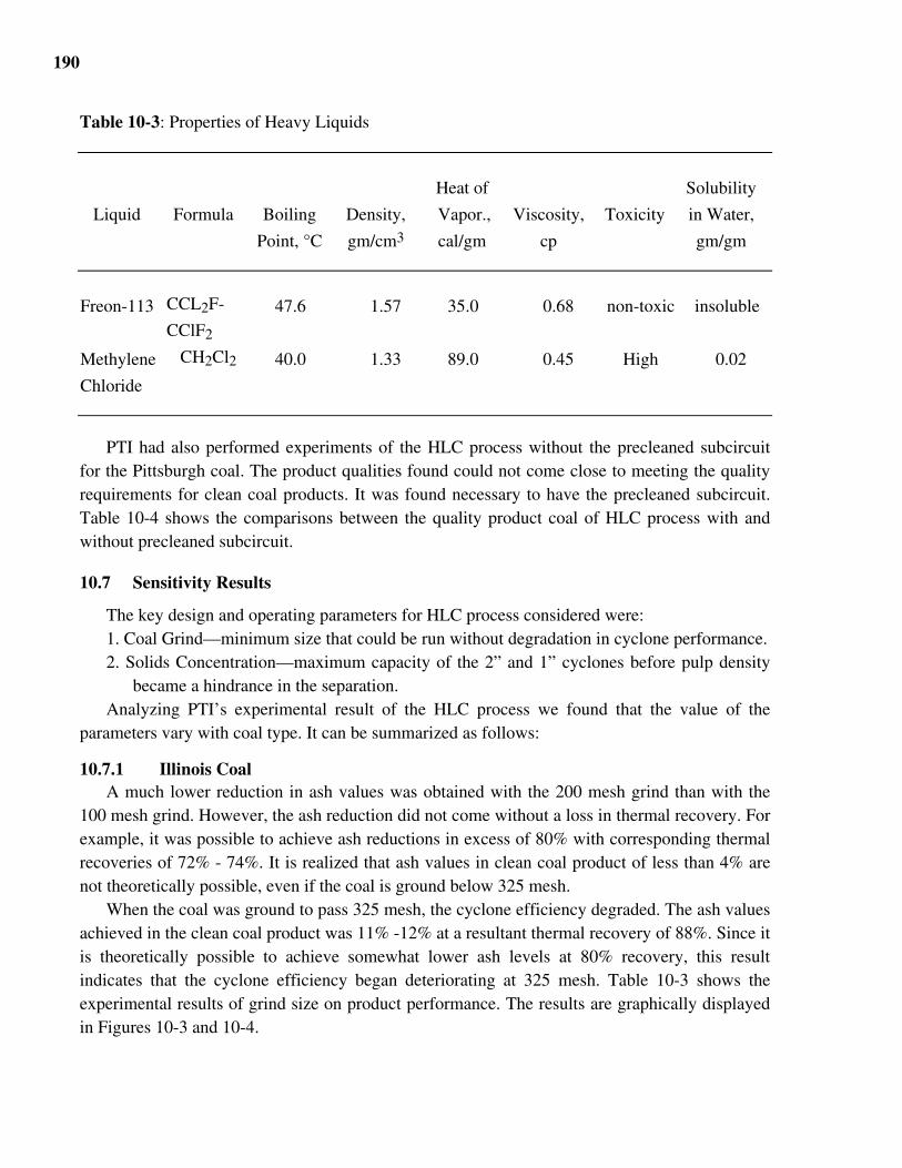
190
Table 10-3: Properties of Heavy Liquids
Liquid Formula Boiling
Point, °C
Density,
gm/cm3
Heat of
Vapor.,
cal/gm
Viscosity,
cp
Toxicity
Solubility
in Water,
gm/gm
Freon-113 CCL2F-
CClF2
47.6 1.57 35.0 0.68 non-toxic insoluble
Methylene
Chloride
CH2Cl2 40.0 1.33 89.0 0.45 High 0.02
PTI had also performed experiments of the HLC process without the precleaned subcircuitfor the Pittsburgh coal. The product qualities found could not come close to meeting the qualityrequirements for clean coal products. It was found necessary to have the precleaned subcircuit.Table 10-4 shows the comparisons between the quality product coal of HLC process with andwithout precleaned subcircuit.
10.7 Sensitivity Results
The key design and operating parameters for HLC process considered were:1. Coal Grind—minimum size that could be run without degradation in cyclone performance.2. Solids Concentration—maximum capacity of the 2” and 1” cyclones before pulp density
became a hindrance in the separation.Analyzing PTI’s experimental result of the HLC process we found that the value of the
parameters vary with coal type. It can be summarized as follows:
10.7.1 Illinois CoalA much lower reduction in ash values was obtained with the 200 mesh grind than with the
100 mesh grind. However, the ash reduction did not come without a loss in thermal recovery. Forexample, it was possible to achieve ash reductions in excess of 80% with corresponding thermalrecoveries of 72% - 74%. It is realized that ash values in clean coal product of less than 4% arenot theoretically possible, even if the coal is ground below 325 mesh.
When the coal was ground to pass 325 mesh, the cyclone efficiency degraded. The ash valuesachieved in the clean coal product was 11% -12% at a resultant thermal recovery of 88%. Since itis theoretically possible to achieve somewhat lower ash levels at 80% recovery, this resultindicates that the cyclone efficiency began deteriorating at 325 mesh. Table 10-3 shows theexperimental results of grind size on product performance. The results are graphically displayedin Figures 10-3 and 10-4.
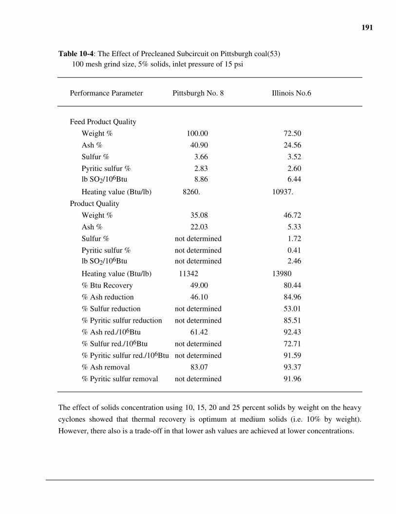
191
Table 10-4: The Effect of Precleaned Subcircuit on Pittsburgh coal(53) 100 mesh grind size, 5% solids, inlet pressure of 15 psi
Performance Parameter Pittsburgh No. 8 Illinois No.6
Feed Product Quality
Weight % 100.00 72.50
Ash % 40.90 24.56
Sulfur % 3.66 3.52
Pyritic sulfur % 2.83 2.60lb SO2/106Btu 8.86 6.44
Heating value (Btu/lb) 8260. 10937.
Product Quality
Weight % 35.08 46.72
Ash % 22.03 5.33
Sulfur % not determined 1.72
Pyritic sulfur % not determined 0.41lb SO2/106Btu not determined 2.46
Heating value (Btu/lb) 11342 13980
% Btu Recovery 49.00 80.44
% Ash reduction 46.10 84.96
% Sulfur reduction not determined 53.01
% Pyritic sulfur reduction not determined 85.51
% Ash red./106Btu 61.42 92.43
% Sulfur red./106Btu not determined 72.71
% Pyritic sulfur red./106Btu not determined 91.59
% Ash removal 83.07 93.37
% Pyritic sulfur removal not determined 91.96
The effect of solids concentration using 10, 15, 20 and 25 percent solids by weight on the heavy
cyclones showed that thermal recovery is optimum at medium solids (i.e. 10% by weight).
However, there also is a trade-off in that lower ash values are achieved at lower concentrations.
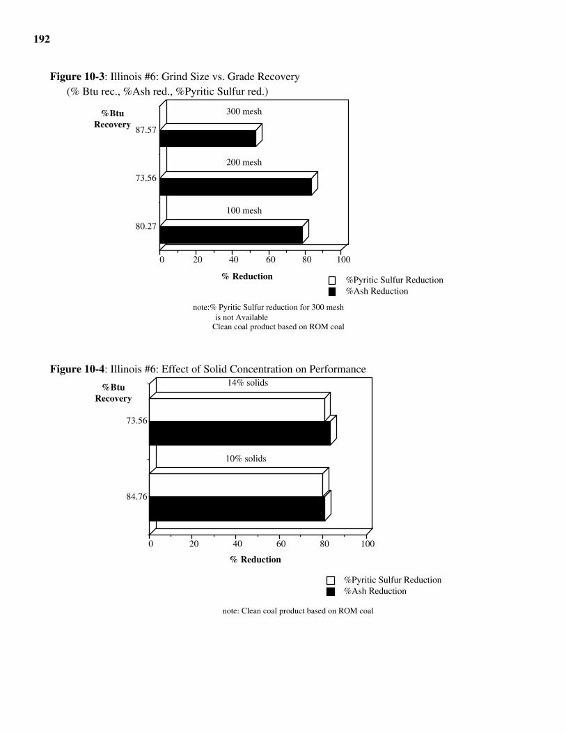
192
Figure 10-3: Illinois #6: Grind Size vs. Grade Recovery(% Btu rec., %Ash red., %Pyritic Sulfur red.)
100806040200
80.27
73.56
87.57
%Ash Reduction%Pyritic Sulfur Reduction% Reduction
%Btu Recovery
300 mesh
200 mesh
100 mesh
note:% Pyritic Sulfur reduction for 300 mesh is not Available
Clean coal product based on ROM coal
Figure 10-4: Illinois #6: Effect of Solid Concentration on Performance
100806040200
84.76
73.56
%Ash Reduction%Pyritic Sulfur Reduction
% Reduction
%Btu Recovery
14% solids
10% solids
note: Clean coal product based on ROM coal
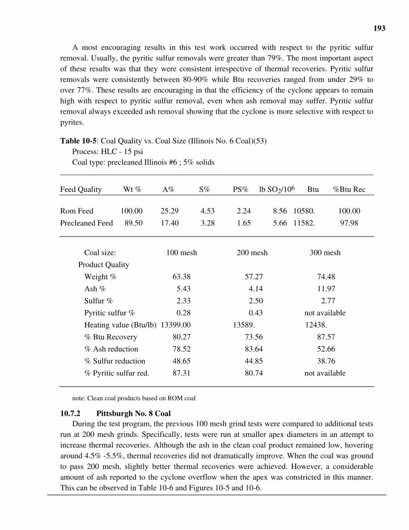
193
A most encouraging results in this test work occurred with respect to the pyritic sulfurremoval. Usually, the pyritic sulfur removals were greater than 79%. The most important aspectof these results was that they were consistent irrespective of thermal recoveries. Pyritic sulfurremovals were consistently between 80-90% while Btu recoveries ranged from under 29% toover 77%. These results are encouraging in that the efficiency of the cyclone appears to remainhigh with respect to pyritic sulfur removal, even when ash removal may suffer. Pyritic sulfurremoval always exceeded ash removal showing that the cyclone is more selective with respect topyrites.
Table 10-5: Coal Quality vs. Coal Size (Illinois No. 6 Coal)(53)Process: HLC - 15 psiCoal type: precleaned Illinois #6 ; 5% solids
______________________________________________________________________________
Feed Quality Wt % A% S% PS% lb SO2/106 Btu %Btu Rec
Rom Feed 100.00 25.29 4.53 2.24 8.56 10580. 100.00
Precleaned Feed 89.50 17.40 3.28 1.65 5.66 11582. 97.98
Coal size: 100 mesh 200 mesh 300 mesh
Product Quality
Weight % 63.38 57.27 74.48
Ash % 5.43 4.14 11.97
Sulfur % 2.33 2.50 2.77
Pyritic sulfur % 0.28 0.43 not available
Heating value (Btu/lb) 13399.00 13589. 12438.
% Btu Recovery 80.27 73.56 87.57
% Ash reduction 78.52 83.64 52.66
% Sulfur reduction 48.65 44.85 38.76
% Pyritic sulfur red. 87.31 80.74 not available
note: Clean coal products based on ROM coal
10.7.2 Pittsburgh No. 8 CoalDuring the test program, the previous 100 mesh grind tests were compared to additional tests
run at 200 mesh grinds. Specifically, tests were run at smaller apex diameters in an attempt toincrease thermal recoveries. Although the ash in the clean coal product remained low, hoveringaround 4.5% -5.5%, thermal recoveries did not dramatically improve. When the coal was groundto pass 200 mesh, slightly better thermal recoveries were achieved. However, a considerableamount of ash reported to the cyclone overflow when the apex was constricted in this manner.This can be observed in Table 10-6 and Figures 10-5 and 10-6.
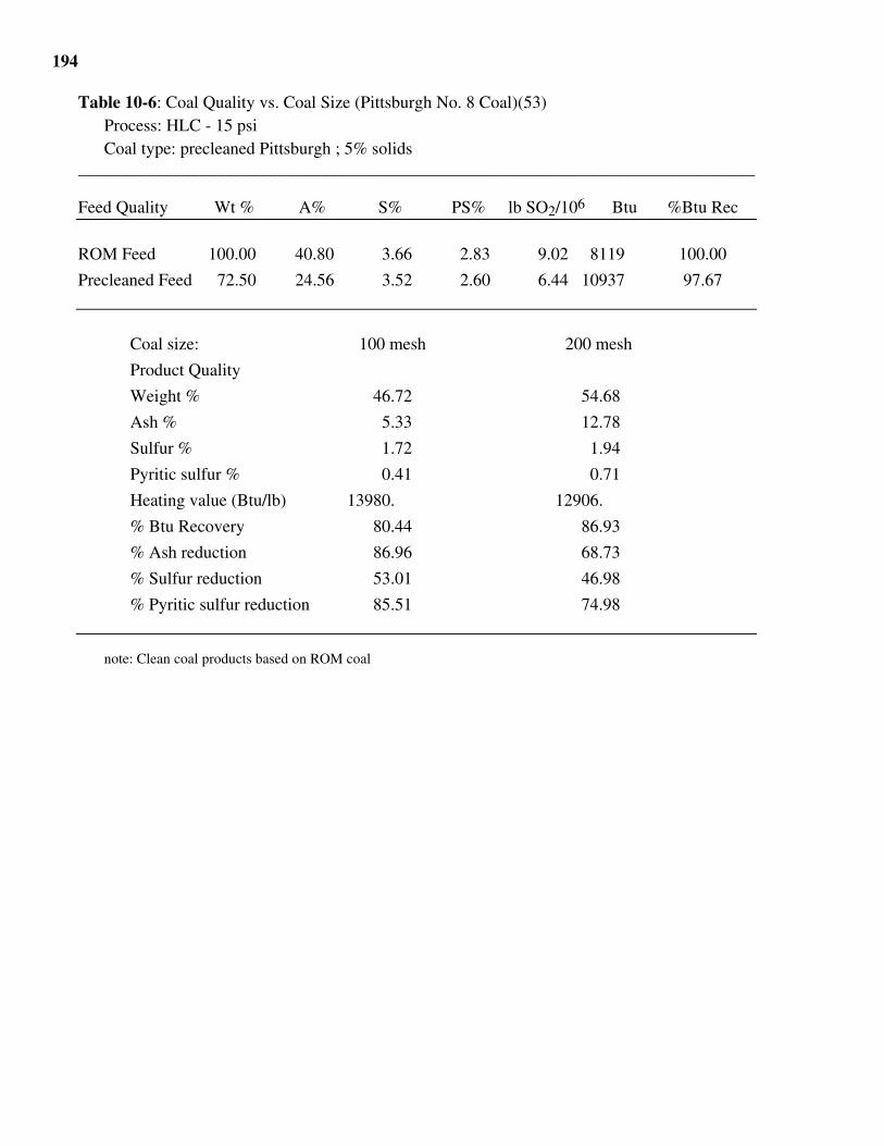
194
Table 10-6: Coal Quality vs. Coal Size (Pittsburgh No. 8 Coal)(53)Process: HLC - 15 psiCoal type: precleaned Pittsburgh ; 5% solids
______________________________________________________________________________
Feed Quality Wt % A% S% PS% lb SO2/106 Btu %Btu Rec
ROM Feed 100.00 40.80 3.66 2.83 9.02 8119 100.00
Precleaned Feed 72.50 24.56 3.52 2.60 6.44 10937 97.67
Coal size: 100 mesh 200 mesh
Product Quality
Weight % 46.72 54.68
Ash % 5.33 12.78
Sulfur % 1.72 1.94
Pyritic sulfur % 0.41 0.71
Heating value (Btu/lb) 13980. 12906.
% Btu Recovery 80.44 86.93
% Ash reduction 86.96 68.73
% Sulfur reduction 53.01 46.98
% Pyritic sulfur reduction 85.51 74.98
note: Clean coal products based on ROM coal
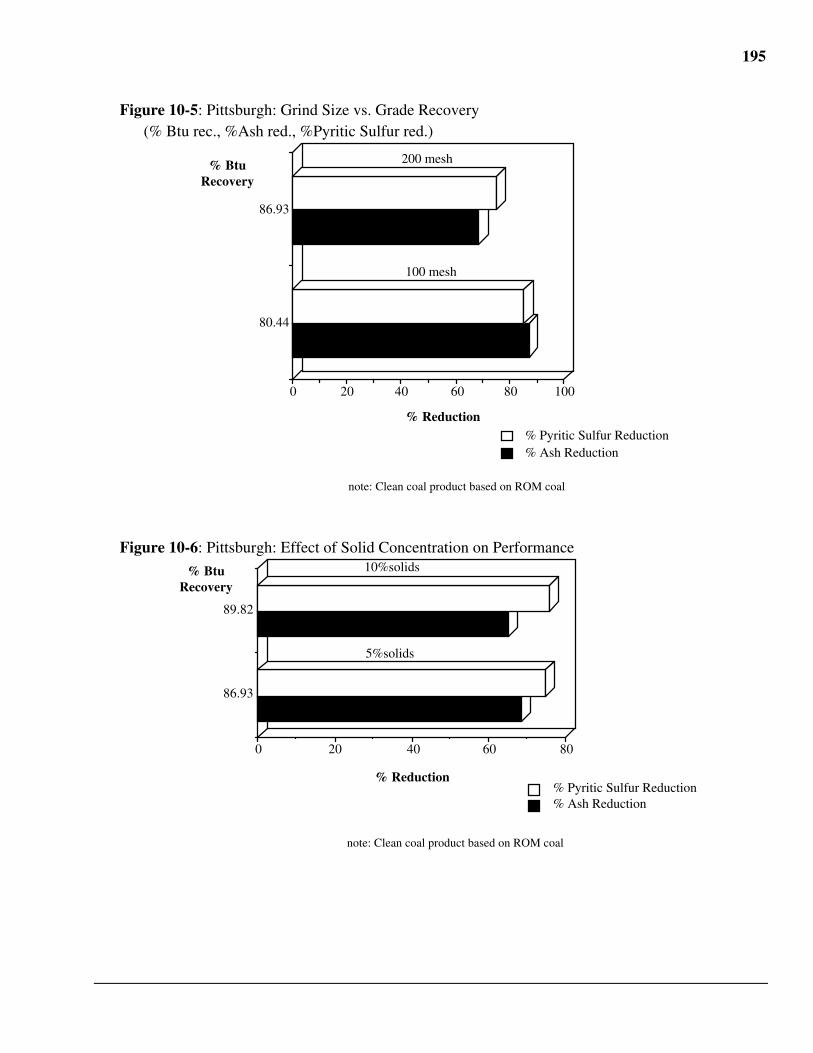
195
Figure 10-5: Pittsburgh: Grind Size vs. Grade Recovery(% Btu rec., %Ash red., %Pyritic Sulfur red.)
100806040200
80.44
86.93
% Ash Reduction% Pyritic Sulfur Reduction
% Reduction
% Btu Recovery
100 mesh
200 mesh
note: Clean coal product based on ROM coal
Figure 10-6: Pittsburgh: Effect of Solid Concentration on Performance
806040200
86.93
89.82
% Ash Reduction% Pyritic Sulfur Reduction
% Reduction
% Btu Recovery
note: Clean coal product based on ROM coal
10%solids
5%solids
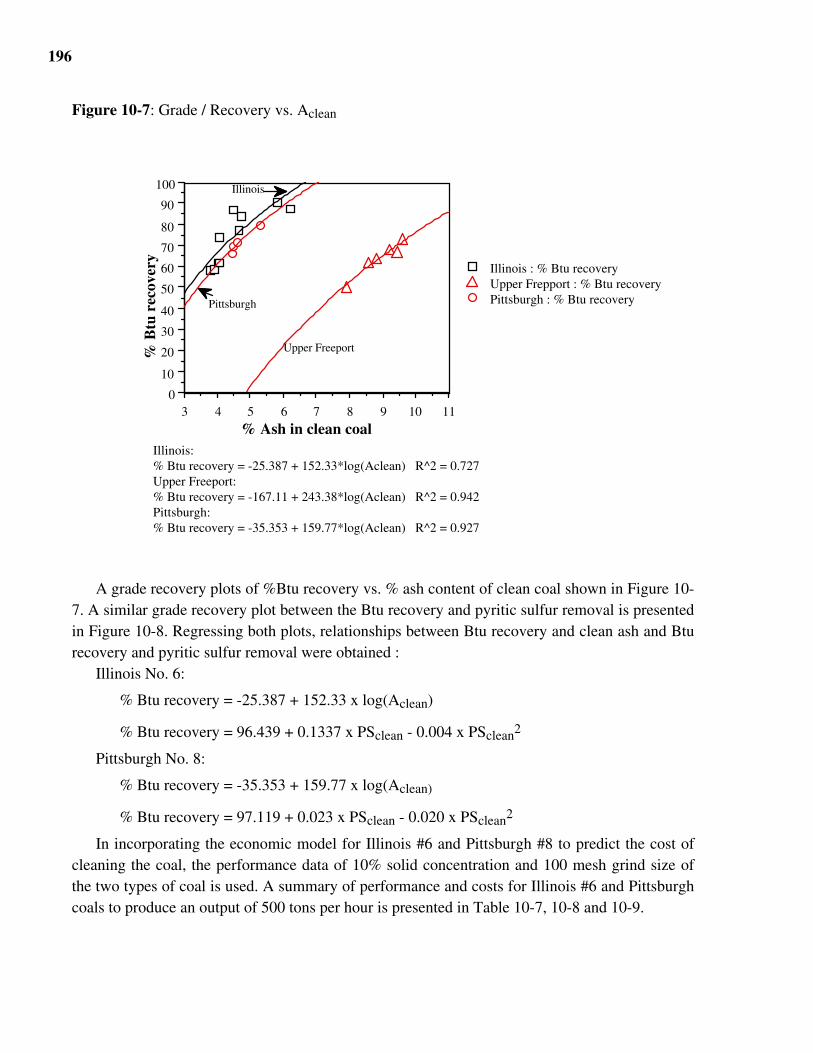
196
Figure 10-7: Grade / Recovery vs. Aclean
111098765430
10
20
30
40
50
60
70
80
90
100
Illinois : % Btu recoveryUpper Frepport : % Btu recoveryPittsburgh : % Btu recovery
% Ash in clean coal
% B
tu r
ecov
ery
Illinois
Pittsburgh
Upper Freeport
Illinois:% Btu recovery = -25.387 + 152.33*log(Aclean) R^2 = 0.727Upper Freeport:% Btu recovery = -167.11 + 243.38*log(Aclean) R^2 = 0.942Pittsburgh:% Btu recovery = -35.353 + 159.77*log(Aclean) R^2 = 0.927
A grade recovery plots of %Btu recovery vs. % ash content of clean coal shown in Figure 10-7. A similar grade recovery plot between the Btu recovery and pyritic sulfur removal is presentedin Figure 10-8. Regressing both plots, relationships between Btu recovery and clean ash and Bturecovery and pyritic sulfur removal were obtained :
Illinois No. 6:
% Btu recovery = -25.387 + 152.33 x log(Aclean)
% Btu recovery = 96.439 + 0.1337 x PSclean - 0.004 x PSclean2
Pittsburgh No. 8:
% Btu recovery = -35.353 + 159.77 x log(Aclean)
% Btu recovery = 97.119 + 0.023 x PSclean - 0.020 x PSclean2
In incorporating the economic model for Illinois #6 and Pittsburgh #8 to predict the cost ofcleaning the coal, the performance data of 10% solid concentration and 100 mesh grind size ofthe two types of coal is used. A summary of performance and costs for Illinois #6 and Pittsburghcoals to produce an output of 500 tons per hour is presented in Table 10-7, 10-8 and 10-9.
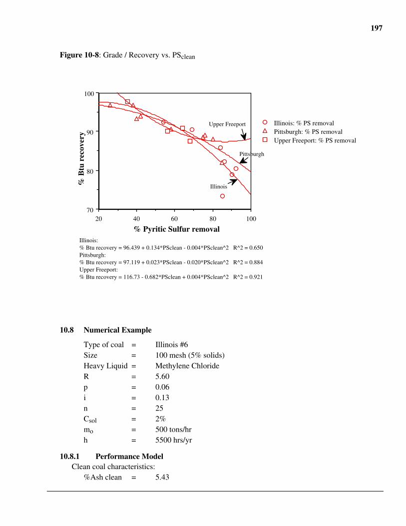
197
Figure 10-8: Grade / Recovery vs. PSclean
1008060402070
80
90
100
Illinois: % PS removalPittsburgh: % PS removalUpper Freeport: % PS removal
% Pyritic Sulfur removal
% B
tu r
ecov
ery
Upper Freeport
Illinois
Pittsburgh
Illinois:% Btu recovery = 96.439 + 0.134*PSclean - 0.004*PSclean^2 R^2 = 0.650Pittsburgh:% Btu recovery = 97.119 + 0.023*PSclean - 0.020*PSclean^2 R^2 = 0.884Upper Freeport:% Btu recovery = 116.73 - 0.682*PSclean + 0.004*PSclean^2 R^2 = 0.921
10.8 Numerical Example
Type of coal = Illinois #6Size = 100 mesh (5% solids)Heavy Liquid = Methylene ChlorideR = 5.60p = 0.06i = 0.13n = 25Csol = 2%mo = 500 tons/hrh = 5500 hrs/yr
10.8.1 Performance ModelClean coal characteristics:
%Ash clean = 5.43
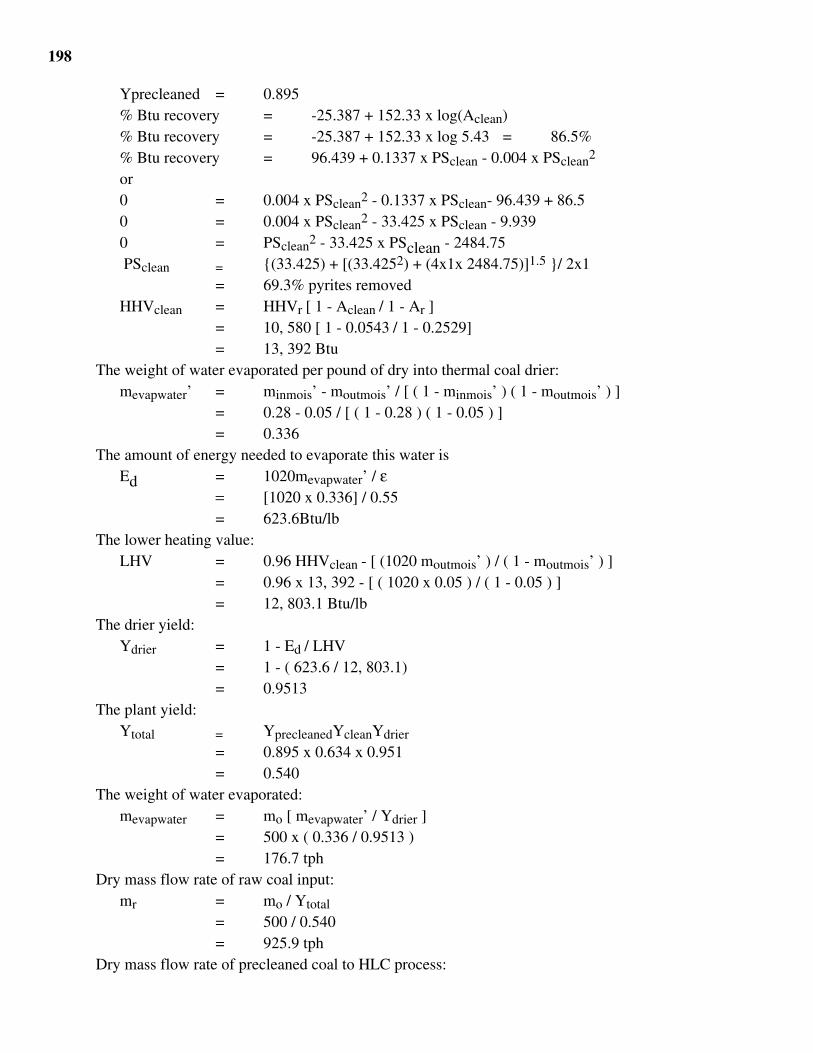
198
Yprecleaned = 0.895% Btu recovery = -25.387 + 152.33 x log(Aclean)% Btu recovery = -25.387 + 152.33 x log 5.43 = 86.5%% Btu recovery = 96.439 + 0.1337 x PSclean - 0.004 x PSclean2
or0 = 0.004 x PSclean2 - 0.1337 x PSclean- 96.439 + 86.50 = 0.004 x PSclean2 - 33.425 x PSclean - 9.9390 = PSclean2 - 33.425 x PSclean - 2484.75 PSclean = {(33.425) + [(33.4252) + (4x1x 2484.75)]1.5 }/ 2x1
= 69.3% pyrites removedHHVclean = HHVr [ 1 - Aclean / 1 - Ar ]
= 10, 580 [ 1 - 0.0543 / 1 - 0.2529]= 13, 392 Btu
The weight of water evaporated per pound of dry into thermal coal drier:mevapwater’ = minmois’ - moutmois’ / [ ( 1 - minmois’ ) ( 1 - moutmois’ ) ]
= 0.28 - 0.05 / [ ( 1 - 0.28 ) ( 1 - 0.05 ) ]= 0.336
The amount of energy needed to evaporate this water isEd = 1020mevapwater’ / ε
= [1020 x 0.336] / 0.55= 623.6Btu/lb
The lower heating value:LHV = 0.96 HHVclean - [ (1020 moutmois’ ) / ( 1 - moutmois’ ) ]
= 0.96 x 13, 392 - [ ( 1020 x 0.05 ) / ( 1 - 0.05 ) ]= 12, 803.1 Btu/lb
The drier yield:Ydrier = 1 - Ed / LHV
= 1 - ( 623.6 / 12, 803.1)= 0.9513
The plant yield:Ytotal = YprecleanedYcleanYdrier
= 0.895 x 0.634 x 0.951= 0.540
The weight of water evaporated:mevapwater = mo [ mevapwater’ / Ydrier ]
= 500 x ( 0.336 / 0.9513 )= 176.7 tph
Dry mass flow rate of raw coal input:mr = mo / Ytotal
= 500 / 0.540= 925.9 tph
Dry mass flow rate of precleaned coal to HLC process:
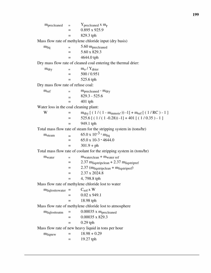
199
mprecleaned = Yprecleaned x mr= 0.895 x 925.9= 829.3 tph
Mass flow rate of methylene chloride input (dry basis)mliq = 5.60 mprecleaned
= 5.60 x 829.3= 4644.0 tph
Dry mass flow rate of cleaned coal entering the thermal drier: mdry = mo / Ydrier
= 500 / 0.951= 525.6 tph
Dry mass flow rate of refuse coal:mref = mprecleaned - mdry
= 829.3 - 525.6= 401 tph
Water loss in the coal cleaning plant:W = mdry [ ( 1 / ( 1 - minmois’)) -1] + mref [ ( 1 / RC ) - 1 ]
= 525.6 [ ( 1 / ( 1 -0.28)) -1] + 401 [ ( 1 / 0.35 ) - 1 ]= 949.1 tph
Total mass flow rate of steam for the stripping system in (tons/hr)msteam = 65.0 x 10⁻³ . mliq
= 65.0 x 10⁻³ . 4644.0= 301.9 + ph
Total mass flow rate of coolant for the stripping system in (tons/hr)mwater = mwaterclean + mwater ref
= 2.37 mliqstripclean + 2.37 mliqstripref
= 2.37 (mliqstripclean + mliqstripref)= 2.37 x 2024.8= 4, 798.8 tph
Mass flow rate of methylene chloride lost to watermliqlosttowater = Csol x W
= 0.02 x 949.1= 18.98 tph
Mass flow rate of methylene chloride lost to atmospheremliqlosttoatm = 0.00035 x mprecleaned
= 0.00035 x 829.3= 0.29 tph
Mass flow rate of new heavy liquid in tons per hourmliqnew = 18.98 + 0.29
= 19.27 tph
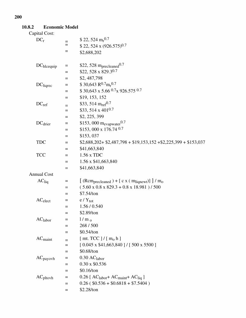
200
10.8.2 Economic ModelCapital Cost:
DCr = $ 22, 524 mr0.7
= $ 22, 524 x (926.575)0.7
= $2,688,202
DChlcequip = $22, 528 mprecleaned0.7
= $22, 528 x 829.30.7
= $2, 487,798DCliqrec = $ 30,643 R0.7mr0.7
= $ 30,643 x 5.66 0.7x 926.575 0.7
= $19, 153, 152DCref = $33, 514 mref0.7
= $33, 514 x 4010.7
= $2, 225, 399DCdrier = $153, 000 mevapwater0.7
= $153, 000 x 176.74 0.7
= $153, 037TDC = $2,688,202+ $2,487,798 + $19,153,152 +$2,225,399 + $153,037
= $41,663,840TCC = 1.56 x TDC
= 1.56 x $41,663,840= $41,663,840
Annual Cost ACliq = [ (Rcmprecleaned ) + [ c x ( mliqnewt)] ] / mo
= ( 5.60 x 0.8 x 829.3 + 0.8 x 18.981 ) / 500= $7.54/ton
ACelect = e / Ytot
= 1.56 / 0.540= $2.89/ton
AClabor = l / m o= 268 / 500= $0.54/ton
ACmaint = [ mt. TCC ] / [ mo h ]= [ 0.045 x $41,663,840 ] / [ 500 x 5500 ]= $0.68/ton
ACpayovh = 0.30 AClabor
= 0.30 x $0.536= $0.16/ton
ACpltovh = 0.26 [ AClabor+ ACmaint+ ACliq ]= 0.26 ( $0.536 + $0.6818 + $7.5404 )= $2.28/ton
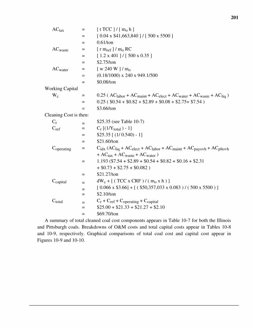
201
ACtax = [ t TCC ] / [ mo h ]= [ 0.04 x $41,663,840 ] / [ 500 x 5500 ]= 0.61/ton
ACwaste = [ r mref ] / mo RC= [ 1.2 x 401 ] / [ 500 x 0.35 ]= $2.75/ton
ACwater = [ w 240 W ] / mo
= (0.18/1000) x 240 x 949.1/500= $0.08/ton
Working CapitalWc = 0.25 ( AClabor + ACmaint + ACelect + ACwater + ACwaste + ACliq )
= 0.25 ( $0.54 + $0.82 + $2.89 + $0.08 + $2.75+ $7.54 )= $3.66/ton
Cleaning Cost is then:Cr = $25.35 (see Table 10-7)Cref = Cr [(1/Ytotal ) - 1]
= $25.35 [ (1/ 0.540) - 1]= $21.60/ton
Coperating = Cidx (ACliq + ACelect + AClabor + ACmaint + ACpayovh + ACpltovh
+ ACtax + ACwaste + ACwater )= 1.193 ($7.54 + $2.89 + $0.54 + $0.82 + $0.16 + $2.31
+ $0.73 + $2.75 + $0.082 )= $21.27/ton
Ccapital = dWc + [ ( TCC x CRF ) / ( mo x h ) ]
= [ 0.066 x $3.66] + [ ( $50,357,033 x 0.083 ) / ( 500 x 5500 ) ]= $2.10/ton
Ctotal = Cr + Cref + Coperating + Ccapital
= $25.00 + $21.33 + $21.27 + $2.10= $69.70/ton
A summary of total cleaned coal cost components appears in Table 10-7 for both the Illinoisand Pittsburgh coals. Breakdowns of O&M costs and total capital costs appear in Tables 10-8and 10-9, respectively. Graphical comparisons of total coal cost and capital cost appear inFigures 10-9 and 10-10.
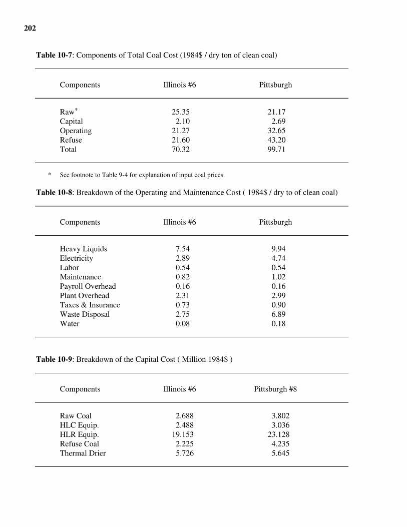
202
Table 10-7: Components of Total Coal Cost (1984$ / dry ton of clean coal)
Components Illinois #6 Pittsburgh
Raw* 25.35 21.17Capital 2.10 2.69Operating 21.27 32.65Refuse 21.60 43.20Total 70.32 99.71
* See footnote to Table 9-4 for explanation of input coal prices.
Table 10-8: Breakdown of the Operating and Maintenance Cost ( 1984$ / dry to of clean coal)
Components Illinois #6 Pittsburgh
Heavy Liquids 7.54 9.94Electricity 2.89 4.74Labor 0.54 0.54Maintenance 0.82 1.02Payroll Overhead 0.16 0.16Plant Overhead 2.31 2.99Taxes & Insurance 0.73 0.90Waste Disposal 2.75 6.89Water 0.08 0.18
Table 10-9: Breakdown of the Capital Cost ( Million 1984$ )
Components Illinois #6 Pittsburgh #8
Raw Coal 2.688 3.802HLC Equip. 2.488 3.036HLR Equip. 19.153 23.128Refuse Coal 2.225 4.235Thermal Drier 5.726 5.645
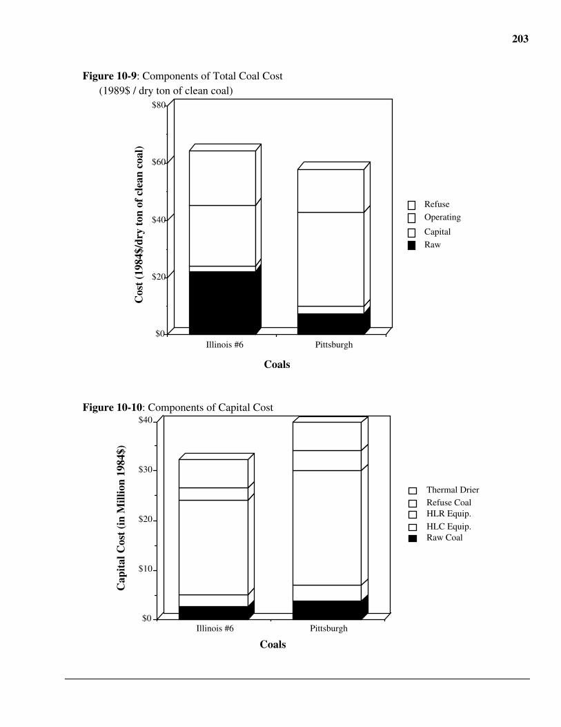
203
Figure 10-9: Components of Total Coal Cost(1989$ / dry ton of clean coal)
Illinois #6 Pittsburgh$0
$20
$40
$60
$80
Raw
Capital
Operating
Refuse
Coals
Cos
t (1
984$
/dry
ton
of
clea
n co
al)
Figure 10-10: Components of Capital Cost
Illinois #6 Pittsburgh$0
$10
$20
$30
$40
Raw CoalHLC Equip.
HLR Equip.Refuse Coal
Thermal Drier
Coals
Cap
ital
Cos
t (i
n M
illio
n 19
84$)
204
11 REFERENCES
1. E. S. Rubin, J. S. Salmento, J. G. Barrett, C. N. Bloyd, H. C. Frey, Modeling andAssessment of Advanced Processes for Integrated Environmental Control of Coal-FiredPower Plants, Prepared by Carnegie Mellon University for DOE/PETC, Pittsburgh, PA(1986).
2. J. S. Salmento, S. Siegel and M. Berkenpas, Center for Energy and EnvironmentalStudies (CEES), Technical Manual for the Integrated Environmental Control Model(IECM), Prepared by Carnegie Mellon University for DOE/PETC, Pittsburgh, PA (1991).
3. Combustion Engineering, Inc., Combustion: Fossil Power Systems. J. G. Singer, Eds.,(Combustion Engineering Inc., Windsor, CT, 1981).
4. U.S. Environmental Protection Agency, Compilation of Air Pollutant Emission Factors,Third Edition (Research Triange Park, NC, 1982).
5. I. Barin, O. Knacke, Thermochemical Properties of Inorganic Substances (Springer-Verlag, New York, NY, 1973).
6. I. Barin, O. Knacke, O. Kubaschewski, Thermochemical Properties of InorganicSubstances: Supplement (Springer-Verlag, New York, NY, 1977), vol. 1.
7. J. Ratafia-Brown, R. Hershey, Science Management Corporation, Modeling of theRegenerator Reactor for the Fluidized Bed Copper Oxide Flue Gas Treatment Process,Report to DOE/PETC, Pittsburgh, PA, (1984).
8. G. H. Babcock, S. Wilcox, Steam/Its Generation and Use (Babcock and WilcoxCompany, New York, NY, 1978).
9. F. P. Incropera, D. P. D. Witt, Fundamentals of Heat Transfer (John Wiley & Sons, NewYork, 1981).
10. ASHRAE Handbook: 1981 Fundamentals (American Society of Heating, Refrigeratingand Air-Conditioning Engineers, Inc., Atlanta, GA, 1981).
11. J. C. Molburg, E.S.Rubin, Air Pollution Control Costs for Coal-to-Electricity Systems,Journal of the Air Pollution Control Association , 33, (1983).
12. Electric Power Research Institute, TAG - Technical Assessment Guide: ElectricitySupply - 1986 (EPRI, Palo Alto, CA, 1986).
13. Electric Power Research Institute, TAG - Technical Assessment Guide: Fundamentalsand Methods Supply-1986 (EPRI, Palo Alto, CA, 1987).
14. J. T. Yeh, C. J. Drummond, Process Simulation of the Fluidized Bed Copper OxideProcess Sulfation Reaction, AIChE 1986 Spring National Meeting (New Orleans, LA,1986).
205
15. J. T. Yeh, R. J. Demski, J. P. Strakey, J. I. Joubert, PETC Fluidized-Bed Copper OxideProcess for Combined SO2/NOx Removal from Flue Gas, AIChE 1984 Winter NationalMeeting (AIChE, Atlanta, GA, 1984).
16. E. S. Rubin, Modeling of Integrated Environmental Control Systems for Coal-FiredPower Plants, Third Quarterly Report to Pittsburgh Energy Technology Center, U.S.Department of Energy, (June, 1988).
17. E. S. Rubin, Modeling of Integrated Environmental Control Systems for Coal-FiredPower Plants, Fourth Quarterly Report to Pittsburgh Energy Technology Center, U.S.Department of Energy, (October, 1988).
18. Science Applications, Inc., NOXSO Corporation, Appendix A: Economic Evaluation ofthe NOXSO Process for Control of Coal Fired Flue Gas NOx and SOx., Report toDOE/PETC, Pittsburgh, PA, (1983).
19. J. L. Halsbeck, L. G. Neal, H. P. Tseng, NOXSO Corporation, Evaluation of the NOXSOCombined NOx/SOx Flue Gas Treatment Process, Report to DOE/PETC, Pittsburgh, PA,(1983).
20. J. L. Halsbeck, C. J. Wang, L. G. Neal, H. P. Tseng, J. D. Tucker, NOXSO Corporation,Evaluation of the NOXSO Combined NOx/SOx Flue Gas Treatment Process, Report toDOE/PETC, Pittsburgh, PA, (1984).
21. J. L. Halsbeck, C. J. Wang, L. G. Neal, C. P. Perng, NOXSO Corporation, Evaluation ofthe NOXSO Combined NOx/SOx Flue Gas Treatment Process, Report to DOE/PETC,Pittsburgh, PA, (1985).
22. R. Keeth, J. E. Miranda, J. B. Reisdorf, R. W. Scheck, Economic Evaluation of FGDSystems , EPRI, Palo Alto, CA, 1986, vol. IV.
23. Private communication with L.G. Neal, NOXSO Corporation (1988).
24. J. L. Halsbeck, L. G. Neal, W. T. Ma, Development Status of the NOXSO CombinedNOx/SO2 Flue Gas Treatment Process, Fourth Symposium on Integrated EnvironmentalControl, EPRI, Palo Alto, CA, (1988).
25. Private Communication with NOXSO Corporation (1988).
26. E. S. Rubin, J. S. Salmento, H. C. Frey, Evaluating Combined SO2/NOx Processes,Fourth Symposium on Integrated Environmental Controls. Co-Sponsored byEPRI/ASME/APCA, EPRI, Palo Alto, CA, (1988).
27. J. L. Halsbeck, L. G. Neal, The NOXSO Process: Simultaneous Removal of SO2 andNOx from Flue Gas, AIChE 1987 Spring National Meeting (Houston, TX, 1987).
28. J. L. Halsbeck, C. J. Wang, The NOXSO Process Development: An Update, Ninth EPA-EPRI Symposium on Flue Gas Desulfurization, EPRI, Palo Alto, CA, (1985).
206
29. D. M. Helfritch, T. L. Feldman, Electron Beam Process Removal of SO2 and NOx fromFlue Gas, Proceedings of 3rd Symposium on Integrated Environmental Controls forFossil Fuel Power Plants (Air Pollution Control Association, Pittsburgh, PA, 1986).
30. H. C. Frey, M.E. Thesis, Department of Mechanical Engineering, Carnegie MellonUniversity (1987).
31. J. Ratafia-Brown, R. Hershey, Economic Evaluation of the Fluidized Bed-Copper OxideFlue Gas Treatment Process and Integrated Sulfuric Acid Plant (Science ManagementCorporation, 1983).
32. J. Ratafia-Brown, R. Hershey, Technical and Economics Evaluation of the Fluidized Bed-Copper Oxide Flue Gas Treatment Process and Integrated Sulfur-Producing Plants,Report to DOE/PETC, Pittsburgh, PA, (Science Management Corporation, 1983).
33. Private Communication from S. Higgins. (St. Louis, MO, Monsanto Enviro-Chem,February 1988).
34. Private Communications from S. Higgins. (St. Louis, MO, Monsanto Enviro-Chem, April1988).
35. C. W. Gibbs, Eds., New Compressed Air and Gas Data (Ingersol-Rand Co., Phillipsburg,1971).
36. C. N. Bloyd, J. C. Molburg, E. S. Rubin, J. F. Skea, The State Level Advanced UtilitySimulation Model Analytical Documentation, Chapter 5: The Pollution Control Module,US EPA, Research Triangle Park, NC, (1984).
37. K. J. Miller, A. W. Deurbrouck, Eds., Froth Flotation to Desulfurize Coal (MarcelDekker, Inc., 1982).
38. D. J. Brown, in Froth Flotation-50th Anniversary Volume D. W. Fuerstenau, Ed. (AIME,New York, 1962) pp. 518-538.
39. F. F. Aplan, in Flotation, A.M. Gaudin Memorial Volume M. C. Feurstenau, Ed. (AIME,New York, 1976), vol. II, pp. 1235-1265.
40. J. W. Leonard, Eds., Coal Preparation, 4th Edition (The American Institute of Mining,Metallurgical and Petroleum Engineers, Inc. (New York, 1979).
41. J. Leja, Surface Chemistry of Froth Flotation (Plenum Press, New York, 1982).
42. T. J. Olson, WEMCO, Froth Flotation for Fine-Coal Cleaning (1985).
43. B. J. Arnold, A Practical View of Rate and Residence Time in Industrial Coal FrothFlotation Circuits, 5th Annual International Pittsburgh Coal Conference, Pittsburgh, PA,(1988).
44. J. A. Avallaro, A. W. Deurbrouck, Froth Flotation Washability Data of VariousAppalachian Coals Using the Timed Release Analysis Technique, United StatesDepartment of the Interior, Bureau of Mines, Washington, DC, (1965).
207
45. B. Onursal, B. Chenz, L. McCandless, Versar, Inc., Cost, Energy and EnvironmentalSensitivity Analysis of Coal Cleaning Technology for Industrial Boiler Applications,Report to US EPA, Research Triangle Park, NC, (1980).
46. Bechtel Corporation, Coal Preparation and Cleaning Assessment Study, Report toArgonne National Lab, Argonne, IL, (1977).
47. J. Buroff, Technology Assessment Report for Industrial Boilers: Coal Cleaning and LowSulfur Coal, Report to US EPA, Research Triangle Park, NC, (Versar, Inc, 1979).
48. Hoffman-Muntner Corporation, Engineering/Economic Analyses of Coal Preparationwith SO2 Cleanup Processes, Interagency Energy-Environment Research andDevelopment Program, US DOE, Washington DC, (1978).
49. J. C. Molburg, Ph.D. Thesis, Department of Engineering and Public Policy, CarnegieMellon University (1982).
50. E.C. Holt, Jr., An Engineering/Economic Analysis of the Coal-Pyrite Flotation Process ,U.S. Department of Energy, Washington DC, (1981).
51. Bechtel Corporation, Advanced Physical Fine Coal Cleaning Spherical Agglomeration,Bechtel Phase I Report to the U.S. Department of Energy, Pittsburgh Energy TechnologyCenter, Pittsburgh, PA, (August, 1988).
52. Burns and Roe Services Corporation, in Acid Rain Control Initiative Coal Preparation—Technical and Economic Analyses , Report to DOE/PETC, Pittsburgh, PA, (March,1987).
53. Process Technology Inc. et al., A Report on Proof of Concept Testing of the HeavyLiquid Cyclone Technology, Report to DOE/PETC, Pittsburgh, PA, (1989).


APPENDIX
Illustrative Case Studies