Modeling of Incident Type and Incident Duration Using Data

Modeling of Incident Type and Incident Duration Using Data from Multiple Years

Sudipta Dey Tirtha

Doctoral Student

Department of Civil, Environmental & Construction Engineering

University of Central Florida

Tel: 407-543-7521

Email: [email protected]

ORCiD number: 0000-0002-6228-0904

Shamsunnahar Yasmin*

Lecturer/Research Fellow

Queensland University of Technology

Centre for Accident Research and Road Safety – Queensland (CARRS-Q) &

Research Affiliate, Department of Civil, Environmental & Construction Engineering, University

of Central Florida

Tel: 61 7 3138 4677; Fax: 61 7 3138 7532


ORCiD number: 0000-0001-7856-5376

Naveen Eluru

Associate Professor

Department of Civil, Environmental & Construction Engineering

University of Central Florida

Tel: 407-823-4815, Fax: 407-823-3315


ORCiD number: 0000-0003-1221-4113

6th June 2020

*Corresponding author

mailto:[email protected]



1

ABSTRACT

The paper presents a model system that recognizes the distinct traffic incident duration profiles

based on incident types. Specifically, a copula-based joint framework has been estimated with a

scaled multinomial logit model system for incident type and a grouped generalized ordered logit

model system for incident duration to accommodate for the impact of observed and unobserved

effects on incident type and incident duration. The model system is estimated using traffic incident

data from 2012 through 2017 for the Greater Orlando region, employing a comprehensive set of

exogenous variables, including incident characteristics, roadway characteristics, traffic condition,

weather condition, built environment and socio-demographic characteristics. In the presence of

multiple years of data, the copula-based methodology is also customized to accommodate for

observed and unobserved temporal effects (including heteroscedasticity) on incident duration.

Based on a rigorous comparison across different copula models, parameterized Frank-Clayton-

Frank specification is found to offer the best data fit for crash, debris, and other types of incident.

The value of the proposed model system is illustrated by comparing predictive performance of the

proposed model relative to the traditional single duration model on a holdout sample.

Keywords: Incident type; Incident duration; Scaled multi-nominal logit; Grouped generalized

ordered logit; Joint framework

2

1 INTRODUCTION

1.1 Background

The prevalence of sub-urban life in North American cities in the latter half of the 20th century and

early 21st century has resulted in an over-reliance on the private vehicle mode. The high private

vehicle dependency burdens existing roadway infrastructure resulting in high congestion levels in

metropolitan areas. Specifically, the economic costs of traffic congestion – direct costs (time and

fuel wastage) and indirect costs (increase in transportation costs) – amount to nearly 305 billion

dollars in 2017 (INRIX, 2018). The annual economic costs add up to nearly $3000 per resident in

large urban regions such as Los Angeles and New York City. Traffic congestion can generally be

attributed to either recurring or non-recurring events. Congestion arising from recurring events is

generally a result of mismatched transportation demand and supply (or capacity). Non-recurring

congestion, on the other hand, is a result of unexpected (or irregular) events such as abandoned

vehicles, adverse weather, spilled loads, highway debris, and traffic crashes. It is estimated that

delays arising from non-recurring congestion contribute between 40 to 60% of total congestion

delays on the US highways (Tavassoli Hojati et al., 2013). Among non-recurring events, the US

Department of Transportation (DOT) reports that traffic incidents alone contribute to 25% of the

total delays leading to an annual loss of about 2.8 billion gallons of gasoline (FHWA EDC, 2012).

The proposed research contributes to reducing traffic congestion on roadways by understanding

the factors influencing incident duration and providing remedial solutions to improve clearance

times.

The overall incident duration, as identified by the Highway Capacity Manual (HCM 2010 ),

is composed of the following four phases: Notification time, Response time, Clearance time and

Traffic recovery time. The first three phases are directly affected by the traffic incident and the

incident management response infrastructure in the urban region. On the other hand, the traffic

recovery time (fourth phase) is a function of total duration of the first three phases and the traffic

demand on the facility. Any improvements in reducing the duration of the first three phases of the

incident will contribute to lower traffic recovery time. The objective of the proposed research effort

is to study the factors influencing incident duration (estimated as the sum of the first three phases)

with a goal of understanding what factors influence incident duration and providing

recommendations for improved traffic incident management plans. Specifically, accurate

estimation of incident duration can allow traffic operations staff to tailor their diversion messages

at the occurrence of an incident.

1.2 Existing Literature

Given the significant influence of traffic incidents on roadways, several research efforts have

examined the factors influencing incident duration focusing either on total duration or the

individual components of duration (see Laman et al., 2018 for a detailed review). The most

commonly employed outcome variable includes total incident duration and duration of individual

incident components (such as notification, response and clearance time).

The methodologies can be broadly classified into two groups: parametric methods and non-

parametric methods. Among parametric methods, the commonly used methodologies include (a)

Linear regression analysis (Garib et al., 2002), (b) Truncated regression based time sequential

method (Khattak et al., 2007), (c) Parametric hazard-based model (Chung, 2010; Junhua et al.,

2013; Tavassoli Hojati et al., 2013, 2014; Ghosh et al., 2014; Chung et al., 2015; Li et al., 2015)

(d) Copula based grouped ordered response model (Laman et al., 2018), (e) Binary probit and

3

regression model based joint framework (Ding et al., 2015). In terms of non-parametric methods,

approaches employed include (a) Tree based model (Valenti et al., 2010; Zhan et al., 2011), (b)

Bayesian networks (Ozbay and Noyan, 2006), (c) Support vector machine (Valenti et al., 2010;

Wu et al., 2011), (d) Artificial neural network (Lee and Wei, 2010), (e) Partial least square

regression (Wang et al., 2013). Based on these models developed, the most important independent

variables identified in literature include: incident characteristics (such as incident type, number of

responders involved, first responder), roadway characteristics (such as functional classification,

geometric characteristics, Average Annual Daily Traffic (AADT), Truck AADT), traffic

conditions (such as time of the day, weekday/weekend), and weather conditions (such as season,

rain, temperature).

1.3 Critique of Earlier Work and Current Study

In earlier studies, while the importance of incident type has been highlighted, it is mostly

considered as an independent variable. The consideration potentially imposes several major

restrictions on the analysis approaches. First, the analysis approaches restrict the influence of

independent variables to be the same across all incident types i.e. the incident duration profile is

restricted to be the same across all incident types. The only variation across incident types is

estimated through the incident type indicator variables. However, it is possible that the impact of

various independent variables is moderated by the incident type indicator. For example, consider

the difference between two incidents: a traffic crash and an abandoned vehicle on roadway. In the

traffic crash event, given the potential possibility of injury (or even fatality), the resource

deployment urgency might be significantly different relative to the abandoned vehicle incident.

This is an example of the same infrastructure availability acting at a different pace based on

incident type. It is plausible to consider that several other independent variable effects are also

affected by incident type.

Second, factors that have led to a particular incident might also affect the incident duration.

For instance, the absence of a shoulder on a roadway facility reduces room for error and might

lead to traffic crashes. The same factor by not allowing adequate room for traffic incident

management vehicles might result in longer incident clearance times. This is an example of an

observed factor (absence of a shoulder) influencing incident type and incident duration. Such

factors can be easily considered in the incident duration model. However, it is also possible that

various unobserved factors that affect incident type might also influence incident duration.

Consider a roadway facility that has a high share of tourist drivers that are unfamiliar with the

roadway. In the presence of tourist drivers, the probability of a traffic crash might be higher. In

this scenario, traffic incident management vehicles might also take longer to arrive at the scene as

the tourist drivers are not aware of the appropriate maneuvers to allow these vehicles. While it is

possible to ascertain locations with higher presence of tourist drivers, it is close to impossible to

determine the exact share of these drivers on roadways. Thus, we have an unobserved factor (share

of tourist drivers) on roadway facility that may affect incident type and incident duration.

Accommodating for the influence of unobserved factors warrants the development of a model

system that examines incident type and incident duration as a joint distribution. Finally, earlier

research typically employed one cross-sectional sample of data for incident duration analysis.

However, with availability of data for several years from various transportation agencies, it is

important to develop model structures that incorporate for the influence of temporal factors

(observed and unobserved) in modeling incident duration.

4

Toward addressing the aforementioned issues, the current study develops a joint model

system with a scaled multinomial logit model (SMNL) system for incident type and a grouped

generalized ordered logit (GGOL) model system for incident duration. The scaled model

accommodates for common unobserved heterogeneity by allowing the variance of the unobserved

component to vary by time period (see Mannering, 2018 for discussion on temporal instability)1.

The grouped generalized ordered system (employed in Laman et al., 2018) offers a flexible non-

linear formulation for modeling duration variables. The approach retains a parametric form similar

to traditional hazard duration models while also allowing for alternative specific effects. The two

model components are stitched together as a joint distribution using the flexible copula-based

approach. In the presence of multiple years of data, the copula-based methodology was also

customized to accommodate for observed and unobserved temporal effects (including

heteroscedasticity) on incident duration. In our analysis, we employ six different copula structures

- the Gaussian copula, the Farlie-Gumbel-Morgenstern (FGM) copula, and set of Archimedean

copulas including Frank, Clayton, Joe and Gumbel copulas (a detailed discussion of these copulas

is available in Bhat and Eluru, 2009). The model system is estimated using traffic incident data

from 2012 through 2017 for the Greater Orlando region. The incident data is augmented with a

host of independent variables including traffic characteristics, roadway characteristics, incident

characteristics, weather conditions, built environment and socio-demographic characteristics.

Further, the value of the proposed model system is illustrated by comparing predictive

performance of the proposed model relative to a single incident duration model (ignoring incident

type profile) on a holdout sample (not used in estimation). The reader would note that such joint

model systems have been employed in travel behavior and transportation safety literature.

However, to the best of the authors’ knowledge, it is the first application in the incident duration

modeling area.

2. ECONOMETRIC METHODOLOGY

The main focus of this paper is to jointly model incident type and incident duration using a copula-

based scaled multinomial logit-group ordered logit model (SMNL-GGOL). In this section,

econometric formulation of the joint model is presented.

2.1 Incident Type Component

Let 𝑞 (𝑞 = 1, 2, … , 𝑄), and 𝑘 (𝑘 = 1, 2, … , 𝐾; 𝐾 = 3) be the indices to represent incident and the

corresponding incident type, respectively. In the joint framework, the modeling of incident type

follows a SMNL model structure. Following the random utility theory, the propensity of an

incident q being incident type k takes the following form:

𝜇𝑞𝑘∗ = 𝛽𝑘𝑥𝑞𝑘 + 𝜉𝑞𝑘 (1)

Where, 𝑥𝑞𝑘 is a vector of independent variables and 𝛽𝑘 is a vector of unknown parameters specific

to incident type 𝑘. 𝜉𝑞𝑘 is an idiosyncratic error term (assumed to be standard type-I extreme value

distributed) capturing the effect of unobserved factors on the propensity associated with incident

type 𝑘. An incident 𝑞 is identified as incident type 𝑘 if and only if the following condition holds:

1 In transportation research domain, most recently, several studies have addressed parameter stability over time (see

Behnood and Mannering (2015), Marcoux et al. (2018), Anowar et al. (2016), Dabbour (2017)). A detailed review of

these articles is beyond of scope of current study. Mannering (2018) presented a detailed discussion on temporal

instability.

5

𝜇𝑞𝑘∗ > 𝑚𝑎𝑥

𝑙=1,2,….,𝐾, 𝑙≠𝐾 𝜇𝑞𝑙

∗ (2)

The functional form presented in Equation (2) can also be represented as binary outcome

models for each incident type k. For example, let 𝜂𝑞𝑘 be a dichotomous variable with binary

outcome 𝜂𝑞𝑘 = 1 if an incident be incident type 𝑘 and 𝜂𝑞𝑘 = 0 if otherwise. Let us define 𝜈𝑞𝑘 as

follows:

𝜈𝑞𝑘 = 𝜉𝑞𝑘 − { 𝑚𝑎𝑥𝑙=1,2,….,𝐾, 𝑙≠𝐾

𝜇𝑞𝑙∗ } (3)

Now, using equation (1), we can rewrite equation (3) as:

𝜈𝑞𝑘 = 𝜇𝑞𝑘∗ − 𝛽𝑘𝑥𝑞𝑘 − { 𝑚𝑎𝑥

𝑙=1,2,….,𝐾, 𝑙≠𝐾 𝜇𝑞𝑙

∗ } (4)

We can update equation (4) as follows

𝜈𝑞𝑘 + 𝛽𝑘𝑥𝑞𝑘 = 𝜇𝑞𝑘∗ − { 𝑚𝑎𝑥

𝑙=1,2,….,𝐾, 𝑙≠𝐾 𝜇𝑞𝑙

∗ } (5)

Now, using Equation (2) we can conclude that the RHS of Equation (5) can be modified as >0,

thus providing the following expression

ηqk = 1 if 𝜈𝑞𝑘 + 𝛽𝑘𝑥𝑞𝑘 > 0 (6)

In Equation (6), probability distribution of incident type outcome depends on distributional

assumption of 𝜈𝑞𝑘, which in turn, depends on distribution of 𝜉𝑞𝑘. Thus, an assumption of

independent and identical Type I Gumbel distribution2 for 𝜉𝑞𝑘 provides a logistic distribution of

𝜈𝑞𝑘. In the presence of multiple years of data, one can also estimate the variance of the error term

with an appropriate base year. To accommodate for this, a scale parameter (𝜑) can be introduced

to form a SMNL model and the probability expression takes the following form:

𝑃𝑟(𝜈𝑞𝑘 < 𝜐) = 𝑒𝑥𝑝 (

−𝜐𝜑

)

𝑒𝑥𝑝 (−𝜐𝜑

) + ∑ 𝑒𝑥𝑝 (𝛽𝑘𝑥𝑞𝑙

𝜑 )

𝑙≠𝑘

(7)

Where, 𝜑 is the scale parameter of interest and is parameterized as exp(𝜚𝜏) and 𝜏 is a set of year

specific factors such as time elapsed variable (computed as the time difference between the

2 The reader would note that under different Generalized Extreme Value distributional assumptions for 𝜉𝑞𝑘 (as

opposed to independent and identical Type I Gumbel distribution) would result in more complex probability

structures for the incident type component with and without closed form expressions.

6

analysis year (2012-2017) from the base year (2012) considered), thus takes the values of 0, 1,

2,3,4 and 5 with 2012 as the base case.

2.2 Incident Duration Component

Let 𝑗𝑘 be the index for the discrete outcome that corresponds to incident duration category for

incident type 𝑘. In joint model framework, incident duration is modelled using a GGOL

specification. In group ordered response model, the discrete incident duration levels (𝑦𝑞𝑘) are

assumed to be associated with an underlying continuous latent variable (𝑦𝑞𝑘∗ ). This latent variable

is typically specified as the following linear equation:

𝑦𝑞𝑘∗ = 𝛼𝑘𝑧𝑞𝑘 + 𝜎𝑗𝑘

+ 휀𝑞𝑘, 𝑦𝑞𝑘 = 𝑗𝑘 if 𝜓𝑗𝑘< 𝑦𝑞𝑘

∗ < 𝜓𝑗𝑘+1 (8)

Where, 𝑧𝑞𝑘 is a vector of exogenous variables for incident type 𝑘 in incident 𝑞, 𝛼𝑘 is row of

unknown parameters, 𝜓𝑗𝑘 is the observed lower bound threshold for time interval level 𝑗𝑘 for

incident type 𝑘. 휀𝑞𝑘 captures the idiosyncratic effect of all omitted variables for incident type 𝑘.

Further, 𝜎𝑗𝑘 is vector of time interval category specific coefficient for time interval alternative 𝑗𝑘

for incident type 𝑘. The 휀𝑞𝑘 terms are assumed identical across incident types. The error terms are

assumed to be independently logistic distributed with variance 𝜆𝑞𝑘2 . The variance vector is

parameterized as follows:

𝜆𝑞𝑘 = 𝑒𝑥𝑝(𝛿 + 𝜌𝑔𝑞𝑘) (9)

Where, 𝛿 is a constant, 𝑔𝑞𝑘 is a set of exogenous variables associated with incident type 𝑘 for an

incident 𝑞 and 𝜌 is the corresponding parameters to be estimated. To be sure, 𝑔𝑞𝑘 also include the

time elapsed variable, thus accommodate the effect of heteroscedasticity within the grouped

ordered framework. The parameterization allows for variance to be different across incidents and

also across time points accommodating heteroscedasticity. The probability for incident type 𝑘 for

time interval in category 𝑗𝑘 is given by:

Pr(𝑦𝑞𝑘 = 𝑗𝑘) = 𝛬 (𝜓𝑗𝑘+1−(𝛼𝑘𝑧𝑞𝑘+𝜎𝑗𝑘

)

𝜆𝑞𝑘) - 𝛬 (

𝜓𝑗𝑘−(𝛼𝑘𝑧𝑞𝑘+𝜎𝑗𝑘

)

𝜆𝑞𝑘) (10)

Where, 𝛬(. ) is the cumulative standard logistic distribution.

2.3 The Joint Model: A Copula Based Approach

The incident type and incident duration components discussed in previous two subsections can be

brought together in the following equation system:

ηqk = 1 if 𝛽𝑘𝑥𝑞𝑘 > −𝜈𝑞𝑘

𝑦𝑞𝑘∗ = 𝛼𝑘𝑧𝑞𝑘 + 𝜎𝑗𝑘

+ 휀𝑞𝑘 if 𝑦𝑞𝑘 = 1[ηqk = 1] 𝑦𝑞𝑘∗

(11)

However, the level of dependency between incident type and duration category of an incident

depends on the type and extent of dependency between the stochastic terms 𝜈𝑞𝑘 and 휀𝑞𝑘. These

dependencies (or correlations) are explored in the current study by using a copula-based approach.

7

In constructing the copula dependency, the random variables (𝜈𝑞𝑘 and 휀𝑞𝑘) are transformed into

uniform distributions by using their inverse cumulative distribution functions, which are then

coupled or linked as a multivariate joint distribution function by applying the copula structure. Let

us assume that 𝛬𝜈𝑘(. ) and 𝛬𝜀𝑘(. ) are the marginal distribution of 𝜈𝑞𝑘 and 휀𝑞𝑘, respectively.

Moreover, 𝛬𝜈𝑘,𝜀𝑘(. ) is the joint distribution of 𝜈𝑞𝑘 and 휀𝑞𝑘. Subsequently, a bivariate distribution

can be generated as a joint cumulative probability distribution of uniform [0, 1] marginal variables

U1 and U2 as below:

𝛬𝜈𝑘,𝜀𝑘(𝜈, 휀) = 𝑃𝑟(𝜈𝑘 < 𝜈, 휀𝑘 < 휀)

= 𝑃𝑟(𝛬𝜈𝑘−1(𝑈1) < 𝜈, 𝛬𝜀𝑘

−1(𝑈2) < 휀)

= 𝑃𝑟(𝑈1 < 𝛬𝜈𝑘(𝜈), 𝑈2 < 𝛬𝜀𝑘(휀))

(12)

The joint distribution (of uniform marginal variable) in Equation (12) can be generated by a

function 𝐶𝜃𝑞(.,.) (Sklar, 1973), such that:

𝛬𝑣𝑘,𝜀𝑘(𝑣, 𝛿2) = 𝐶𝜃𝑞(𝑈1 = 𝛬𝑣𝑘(𝑣), 𝑈2 = 𝛬𝜀𝑘(휀)) (13)

Where, Cθq(. , . ) is a copula function and θq the dependence parameter defining the link between

vqk and εqk. It is important to note here that, the level of dependence between incident type and

incident duration level can vary across incidents. Therefore, in the current study, the dependence

parameter θq is parameterized as a function of observed incident attributes as follows:

𝜃𝑞 = 𝑓𝑛(𝛾𝑘𝑠𝑞𝑘) (14)

Where, sqk is a vector of exogenous variable, γk is a vector of unknown parameters (including a

constant) specific to incident type 𝑘 and 𝑓𝑛 represents the functional form of parameterization. In

our analysis, six different copulas structure – Gaussian, FGM, Frank, Clayton, Joe and Gumbel

copulas are employed. Based on the dependency parameter permissible ranges, alternate

parameterization forms for the six copulas are considered in our analysis. For Normal, FGM and

Frank Copulas, we use θq = γksqk, for the Clayton copula we employ θq = exp (γksqk), and for

Joe and Gumbel copulas we employ θq = 1 + exp (γksqk).

2.3.1 Estimation Procedure

The joint probability that the incident 𝑞 is identified to be incident type 𝑘 and the resulting incident

duration level 𝑗𝑘, from equation (7) and (10), can be written as:

𝑃𝑟(𝜂𝑞𝑘 = 1, 𝑦𝑞𝑘 = 𝑗𝑘)

= 𝑃𝑟 {(𝛽𝑘𝑥𝑞𝑘 > −𝑣𝑞𝑘), ((𝜓𝑗𝑘−1 − (𝛼𝑘𝑧𝑞𝑘 + 𝜎𝑗𝑘

)

𝜆𝑞𝑘) < 휀𝑞𝑘 < (

𝜓𝑗𝑘− (𝛼𝑘𝑧𝑞𝑘 + 𝜎𝑗𝑘

)

𝜆𝑞𝑘))}

= 𝑃𝑟 {(𝑣𝑞𝑘 > −𝛽𝑘𝑥𝑞𝑘), ((𝜓𝑗𝑘−1 − (𝛼𝑘𝑧𝑞𝑘 + 𝜎𝑗𝑘

)

𝜆𝑞𝑘) < 휀𝑞𝑘 < (

𝜓𝑗𝑘− (𝛼𝑘𝑧𝑞𝑘 + 𝜎𝑗𝑘

)

𝜆𝑞𝑘))}

(15)

8

= 𝑃𝑟 ((𝑣𝑞𝑘 > −𝛽𝑘𝑥𝑞𝑘), (휀𝑞𝑘 < (𝜓𝑗𝑘

− (𝛼𝑘𝑧𝑞𝑘 + 𝜎𝑗𝑘)

𝜆𝑞𝑘)))

− 𝑃𝑟 ((𝑣𝑞𝑘 > −𝛽𝑘𝑥𝑞𝑘), (휀𝑞𝑘 < (𝜓𝑗𝑘−1 − (𝛼𝑘𝑧𝑞𝑘 + 𝜎𝑗𝑘

)

𝜆𝑞𝑘)))

= 𝛬𝜀𝑘 ((𝜓𝑗𝑘

−(𝛼𝑘𝑧𝑞𝑘+𝜎𝑗𝑘)

𝜆𝑞𝑘)) − 𝛬𝜀𝑘 ((

𝜓𝑗𝑘−1−(𝛼𝑘𝑧𝑞𝑘+𝜎𝑗𝑘)

𝜆𝑞𝑘)) − (𝑃𝑟 [𝑣𝑞𝑘 < −𝛽𝑘𝑥𝑞𝑘 , 휀𝑞𝑘 <

(𝜓𝑗𝑘

−(𝛼𝑘𝑧𝑞𝑘+𝜎𝑗𝑘)

𝜆𝑞𝑘) ] − 𝑃𝑟 [𝑣𝑞𝑘 < −𝛽𝑘𝑥𝑞𝑘 , 휀𝑞𝑘 < (

𝜓𝑗𝑘−1−(𝛼𝑘𝑧𝑞𝑘+𝜎𝑗𝑘)

𝜆𝑞𝑘)] )

The joint probability of Equation (15) can be expressed by using the copula function in

equation (13) as:

𝑃𝑟(𝜂𝑞𝑘 = 1, 𝑦𝑞𝑘 = 𝑗𝑘)

= 𝛬𝜀𝑘 (𝜓𝑗𝑘

− (𝛼𝑘𝑧𝑞𝑘 + 𝜎𝑗𝑘)

𝜆𝑞𝑘) − 𝛬𝜀𝑘 ((

𝜓𝑗𝑘−1 − (𝛼𝑘𝑧𝑞𝑘 + 𝜎𝑗𝑘)

𝜆𝑞𝑘))

− [𝐶𝜃𝑞(𝑈𝑞,𝑗𝑘 , 𝑈𝑞

𝑘) − 𝐶𝜃𝑞(𝑈𝑞,𝑗−1𝑘 , 𝑈𝑞

𝑘)]

(16)

Thus, the likelihood function with the joint probability expression in equation (16) for

incident type and duration level outcomes can be expressed as:

𝐿 = ∏ [∏ ∏{𝑃𝑟(𝜂𝑞𝑘 = 1, 𝑦𝑞𝑘 = 𝑗𝑘)} 𝜔𝑞𝑗𝑘

𝐽

𝑗=1

𝐾

𝑘=1

]

𝑄

𝑞=1

(17)

where, ωqjk is dummy with ωqjk = 1 if the incident 𝑞 sustains incident type 𝑘 and an incident

duration level of 𝑗 and 0 otherwise. All the parameters in the model are then consistently estimated

by maximizing the logarithmic function of L. The parameters to be estimated in the model are: βk

and 𝜚 in the SMNL model component, 𝛼𝑘 and 𝜓𝑗𝑘 in GGOL model component, and finally γk in

the dependency component.

3 DATA DESCRIPTION The main data source for the current study is the incident management dataset compiled by the

Florida Department of Transportation (FDOT). Event management data collected over six years

from 2012 to 2017 for Greater Orlando region was processed to prepare the final dataset. The study

region consists of a number of major highways of the Greater Orlando Region including Interstate

- 4 (I-4), East-West expressway (toll road 408), Beachline expressway (toll road 528), Central

Florida Greenway (toll road 417), Daniel Webster Western Beltway (toll road 429) and other

arterials, collectors and local roads.

9

FIGURE 1 Distribution of Incident Duration for Different Incident Types

The study is confined to the incidents with an official reported response compiled by FDOT.

The final dataset, after removing events without any response, consists of 326,348 incident records.

In preparation of estimation sample, 2000 incidents were randomly sampled for each year (2012

to 2017), to create an overall estimation sample of 12,000 records. For validation test, on the other

hand, 2500 records from each year were sampled randomly from the unused data resulting in a

validation dataset of 15,000 records. Three incident types indicating crash, debris and other

incidents were considered. Other incidents include disabled vehicles, abandoned vehicle, and tire

blown. Initial model estimation efforts considered “other category” as separate categories.

However, the model estimation results indicated the absence of substantial differences between

disabled, abandoned and tire blown categories. Hence, these alternatives were merged in the other

category. For incident duration, we have considered 10 categories (>0-5, >5-10, >10-15, >15-20,

>20-25, >25-30, >30-50, >50-80, >80-120 and >120minute). Distribution of incident duration

categories for each incident type is presented in Figure 1. From Figure 1, we can observe that

incident duration profile varies substantially across different incident type categories. Crash events

has a left skewed duration distribution while the other two incident types have a right skewed

distribution. Given these clear differences across the three incident types, developing a single

duration model (as considered in existing literature) can potentially result in biased and incorrect

parameter estimation.

3.1 Independent Variables

The incident management dataset is augmented with several exogenous variables. These variables

are sourced from American Community Survey, Florida Geographic Data Library, FDOT and

Florida Automated Weather Network databases. Exogenous variables considered can be classified

into six broad categories: incident characteristics, traffic characteristics, roadway characteristics,

weather conditions, built environment and socio-demographic characteristics. Incident

characteristics include number of responders, first responder and notified agency. Roadway

characteristics considered include location in terms of intersection and interchange, roadway’s

functional class, geometric characteristics, average annual daily traffic (AADT). Traffic

characteristics include time of the day to accommodate hourly variation of traffic and

weekday/weekend. Weather condition include season and rain. Built environment characteristics

include land-use mix variable, number of business centers, commercial establishment, recreational

0

20

40

60

80

100

PE

RC

EN

TA

GE

DURATION LEVELS (IN MINUTES)

Crash Debris Other Incidents

10

establishment, restaurants and other establishments in 0.5mile buffer area of each incident. Socio-

demographic characteristics include population and median income in the 0.5mile buffer area.

Built environment and socio-demographic variables are computed for the 0.5 miles buffers area of

each incident location by using ArcGIS. The descriptive statistics of exogenous variables found

significant in the final specified model are presented in Table 1.

TABLE 1 Description of Model Estimation Sample

Variable Variable Description Freq. Percentage

(%)

Dependent Variable for Incident Type Component

Crash 2044 17.033

Debris 2197 18.308

Others type of incidents 7759 64.658

Dependent Variable for Incident Duration Component

Incident duration category 1 -T1 >0-5minute 4353 36.275









Incident duration category 10 -

T10 >120minute 1268 10.567

Independent Variables (Categorical)

Incident Characteristics

First responder

Road Ranger First responder is the Road Rangers 10417 86.808

Other agencies First responder is Other agencies 1583 13.192

Notified Agency

Road Ranger (RR) Incidents were notified to the Road Rangers 5248 43.733

Other agencies Incidents were notified to the Other agencies 6752 56.267

Roadway Characteristics

At interchange or not

At interchange Incident was identified on an interchange 1323 11.025

Non-interchange Incident was not identified on an interchange 10677 88.985

At intersection or not

At intersection Incident was identified on an intersection 3055 25.458

Non-intersection Incident was not identified on an intersection 8945 74.542

Functional Classification

Rural Highway Incident was identified on rural highway 803 6.692

Rural Arterial Incident was identified on rural arterial 485 4.042

Rural Local Incident was identified on rural local road 53 0.442

11

Urban Interstate Incident was identified on urban interstate 3535 29.458

Urban Freeway Incident was identified on urban freeway 2980 24.833

Urban Arterial Incident was identified on urban arterial 2065 17.208

Urban Local Incident was identified on urban local road 2079 17.325

Posted speed limit

Speed limit<55 Posted speed limit is less than or equal to

55mph 4913 40.942

Speed limit>55 Posted speed limit is higher than 55mph 7087 59.058

Traffic Condition

Weekend/Weekday

Weekday Monday - Friday 9196 76.633

Weekend Saturday and Sunday 2804 23.367

Time of the day

6am – 9am 1822 15.183

9am – 4pm 5151 42.925

4pm – 6pm 1877 15.642

6pm – 9pm 1826 15.217

9pm – 6am 1325 11.042

Weather Condition

Season

Spring March, April and May 2910 24.25

Summer June, July and August 3193 26.608

Fall September, October and November 3124 26.033

Winter December, January and February 2773 23.108

Independent Variables (Ordinal)

Variable Mean Min/Max

Incident Characteristics

No. of responders No. of responders involved in clearance 1.175 1.000/8.000

Time elapsed Time since 2012 in year 2.500 0.000/5.000

Independent Variables (Continuous)


AADT Ln(AADT/10000) 1.421 0.030/3.033

Inside shoulder Ln(Inside shoulder width in ft) 2.056 0.693/3.611

Outside shoulder Ln(Outside shoulder width in ft) 2.009 0.693/3.045

Median width Ln(Median width in ft) 3.698 1.099/5.889

Weather Condition

Rain Amount of rain in inch at the hour of incident

occurrence 0.006 0.000/1.617

Built Environment

Business Ln(No. of business establishments in 0.5mile

buffer) 0.101 0.000/1.609

Commercial Ln(No. of commercial establishment in 0.5mile

buffer) 0.095 0.000/1.792

Recreational Ln(No. of recreational establishment in 0.5mile

buffer) 0.271 0.000/2.565

12

Restaurant Ln(No. of restaurants in 0.5mile buffer) 1.111 0.000/4.357

CBD distance Ln(Distance from central business district in

miles) 1.754 -2.182/3.444

Land-use mix

Land-use in computed as −𝛴𝑘(𝑝𝑘(ln 𝑝𝑘))

𝑙𝑛 𝑁, where

𝒌 is the category of land-use, 𝒑 is the

proportion of the developed land area, 𝑵 is the

number of land-use categories within a buffer

0.377 0.000/0.963

Socio-demographic Characteristics

Population Ln(Total population in 0.5mile buffer) 6.805 2.652/8.721

Median income Ln(Average median income in 0.5mile buffer

in thousand) 4.211 3.488/4.997

4. MODEL SELECTION

The empirical analysis involves the estimation of models by using six different copula structures:

a) FGM, b) Frank, c) Gumbel, d) Clayton, e) Joe and f) Gaussian copulas. A series of models have

been estimated in the current study context. First, an independent copula model (separate SMNL

and GGOL models) is estimated to establish a benchmark for comparison. Second, 6 different

models that restricted the copula dependency structure across the three incident types and incident

duration models to be the same are estimated. Third, based on the copula parameter significance

for each incident type, copula models that allow for different dependency structures for different

incident type and incident duration combinations are estimated (for example Frank copula for the

first two incident types and Clayton copula for other incident type). Fourth, joint models with

different copula profiles are further augmented by parameterizing the copula profiles. Finally, to

determine the most suitable copula model (including the independent copula model), a comparison

exercise is undertaken. The alternative copula models estimated are non-nested and hence, cannot

be tested using traditional log-likelihood (LL) ratio test. We employ the Bayesian Information

Criterion (BIC) to determine the best model among all copula models without parameterization.

The computed BIC (LL, Number of parameters) value of the independent model is

62434.01 (-30709.80, 108). With single copula dependency structure, the best model fit is obtained

for Frank with BIC value of 62336.31 (LL = -30698.50, No. of parameters = 100). However, the

lowest BIC value is obtained for a combination model of Frank-Clayton-Frank copulas (Frank

copula structure for crash and other incident types and Clayton dependency structure for debris)

and the BIC value is found to be 62335.11 (LL = -30697.92, No. of parameters = 100).

Subsequently, the copula profile for the Frank-Clayton-Frank model has been parameterized. The

copula model with and without parameterizations are nested within each other and can be

compared by employing log-likelihood ratio test. The LL value for the parameterized Frank-

Clayton-Frank copula model is found to be LL = -30693.72 (No. of parameters = 101, BIC =

62336.10). The log-likelihood ratio test yields a test statistic value of 8.40 which is substantially

larger than the critical chi-square value (6.635) with 1 degrees of freedom at 99% level of

significance. Thus, the comparison exercise confirms the importance of allowing the dependency

profile to vary across different records. In presenting the effects of exogenous variables in the joint

model specification, we will restrict ourselves to the discussion of the Frank-Clayton-Frank

specification with parameterization.

13

5 MODEL RESULTS

5.1 Incident Type Model Component

Table 2 provides parameter estimates of incident type model component. A positive (negative)

value of the parameters in Table 2 indicates higher (lower) propensity of the corresponding

incident category compared to the base category.

5.1.1 Roadway Characteristics

Among roadway characteristics, interchange variable impact indicates that at interchange

locations, the likelihood of debris incidence is higher while at intersections, the likelihood of

crashes is higher. Incidents on rural highways are more likely to be crashes while less likely to be

debris. The relationship is reversed for rural arterials. For rural local roads, crash incidences are

found to be higher. On urban interstate, the results indicate higher possibility for crash and a lower

possibility for debris incidents. The relationship is reversed for urban freeways. On urban arterials,

the possibility of crash incident type is likely to be higher.

Estimation result for posted speed limit indicates that the roadway speed limit being greater

than 55 has a negative impact on the likelihood of crash incidence and positive influence on debris

incidence. Parameter estimate for AADT indicates that increasing AADT is likely to reduce the

possibility of Debris incidences. Shoulder width and median width variables have significant

impacts on incident types. Specifically, with the increase in inside shoulder width, the probability

of crash incidence is found to be higher. On the other hand, increasing width of the outside shoulder

is likely to reduce the possibility of crash and debris incidents. This is expected because with

increasing outside shoulder width more space for disabled or abandoned vehicles is available (a

major share of the Other alternative). Median width variable is negatively associated with crash

and positively associated with debris incidents.

5.1.2 Traffic Characteristics

Traffic characteristics prior to the occurrence of incident might affect the potential incident type.

However, it is not feasible to generate detailed traffic information across all the incident records

considered in our analysis. Hence, as potential surrogates reflecting traffic conditions, we

considered the time period and day of the week. The results indicate that all time periods from 6

am – 9 pm are less likely to result in crash. The possibility of crashes is particularly lower in the

time period 9 am – 4 pm. At the same time, the results indicate that debris incidences are more

likely to occur during the 6 am – 9 pm time period. The probability is particularly higher for debris

during time period 6 am – 4 pm. Finally, the day of the week parameters indicate that the likelihood

of debris incidence is lower on weekdays (relative to weekends).

5.1.3 Weather Conditions

The variables tested for seasonality resulted in a significant parameter for spring. The result

indicates lower propensity for crash during spring season. The results for Rain variable indicate

that in the presence of rain, crash incidences are likely to be higher. The result is expected in

Florida with tropical weather where heavy showers appear in short time frame affecting overall

road safety.

14

5.1.4 Built Environment

Incident type is affected by crash proximity to central business district (CBD). Specifically, as the

distance of the incident location to CBD increases the likelihood of crash and debris increases.

Several land-use variables affect incident type likelihood. Business and restaurant land use

contribute to lower debris incidence while recreational land use contributes to higher debris

incidence. Commercial and restaurant land use contribute to higher crash possibilities. Finally,

overall land-use mix variable is found to have a positive effect on debris variable.

5.1.5 Socio-demographic Variables

Population density and median income in the proximity of incident are found to be significant

predictors of incident type. Higher population density increases probability of an incident being

debris and reduces the likelihood of an incident being crash relative to other incidents. The result

is reflective of the enhanced safety in highly populated areas. Similarly, incidents occurring in

high income areas are less likely to be a crash.

5.1.6 Scale parameter

To accommodate for difference in incident type with time, we generated the time elapsed variable

(time since 2012). The estimated model result indicates that the variance of the error term for the

time elapsed variable increases with time highlighting the impact of unobserved time specific

factors.

TABLE 2 Parameter Estimates for Incident Type Component (SMNL Model Results)

Variable Crash Debris Other Incidents

Est. t-Stat Est. t-Stat Est. t-Stat

Constant 7.6596 9.9390 -5.9350 -10.2680 -- --


At Interchange or not (Base: Non-interchange)

At interchange --1 -- 0.9211 9.9460 -- --

At intersection or not (Base: Non-intersection)

At intersection 0.1787 2.176 -- -- --

Function class of roadway (Base: Urban Local)

Rural highway 0.4979 2.601 -0.5990 -2.048 -- --

Rural arterials -1.2389 -4.3970 0.9905 4.5440 -- --

Rural local 2.2113 4.3770 -- -- -- --

Urban interstate 0.8258 5.7170 -0.8513 -5.122 -- --

Urban Freeway -0.5846 -3.7250 1.5622 11.709 -- --

Urban arterials 0.4458 4.5400 -- -- -- --

Posted speed limit (Base: Speed limit<55)

Speed limit>55 -0.4219 -3.8180 0.3847 3.6670 -- --

AADT -- -- -0.2971 -4.8940 -- --

Inside shoulder 0.1585 2.1560 -- -- -- --

Outside shoulder -0.1880 -2.3040 -0.4233 -5.878 -- --

15

Median width -0.5487 -8.7420 0.1502 1.9980 -- --

Traffic Condition

Time of the day (Base: 9pm – 6am)

6am – 9am -0.2782 -2.3850 1.5825 7.0290 -- --

9am – 4pm -0.6918 -7.2730 1.5318 7.1820 -- --

4pm – 6pm -0.2568 -2.3760 1.1637 5.1630 -- --

6pm – 9pm -0.4600 -4.2390 0.9021 3.9670 -- --

Weekend/ Weekday (Base: Weekend)

Weekday -- -- -0.4261 -5.4610 -- --

Weather Conditions

Season (Base: Other seasons)

Spring -0.2338 -3.1960 -- -- -- --

Rain 2.2397 4.1600 -- -- -- --

Built Environment

CBD Distance 0.3397 6.9950 0.3598 5.1390 -- --

Business -- -- -1.1775 -7.3720 -- --

Commercial

0.6877 5.8180 -- -- -- --

Recreational

-- -- 0.3336 4.0340 -- --

Restaurants 0.1346 4.4310 -0.1513 -3.9760 -- --

Land-use mix -- -- 0.4499 2.6560 -- --

Socio-demographic

Population -0.4200 -8.4150 0.3749 6.7340 -- --

Median income -1.1809 -9.2630 -- -- -- --

Scale Parameter

Time elapsed Estimate = 0.0895 (t-stat = 10.4950)

1-- = Attributes insignificant at 90% confidence level

5.2 Incident Duration Model Component

Table 3 provides parameter estimates of the duration model for crash, debris and other incident

type categories considered in the study. A positive (negative) value of the parameter in Table 3

indicates propensity for higher (lower) duration.

5.2.1 Incident Characteristics

Several incident characteristics such as number of responders, category of the first responder and

notified agency are found to influence incident duration. In terms of number of responders, the

incident duration is found to be higher with the increased number of responders for all duration

models. The result might seem counterintuitive. However, the increase in the number of responders

is representative of the seriousness of the incident. Thus, based on incident notification, for more

serious incidents, a large number of responders are likely to arrive at a scene for assisting in

incident clearance. Several agencies are involved in the incident notification and clearance

activities. The results indicate that if Road Ranger is the notified agency then the incident durations

16

are likely to be lower for debris and other incidents (see (Laman et al., 2018) for similar result).

Incident durations are also found to be lower for all incident categories if Road Ranger is the first

responder.

5.2.2 Roadway Characteristics

The roadway characteristics are found to have no impact on incident duration for crashes. The

result is a reflection of the emphasis on crash incident clearance. The emphasis is warranted given

the potential savings of life in the event of crash. For debris, the duration is likely to be longer on

rural arterials. For other incidents, the roadway classification of rural arterials and urban freeways

are found to have negative impact on the duration component. The results from our models are

different from earlier research (Ghosh et al., 2014; Laman et al., 2018) and warrant further

investigations. Roadway geometric characteristics are found to have no effect on incident duration

for any incident categories.

5.2.3 Traffic Characteristics

For crash and debris, the model estimation results indicate that incident durations are likely to be

higher during 9 pm to 6 am (see (Chung, 2010) and (Laman et al., 2018) for similar findings). On

the other hand, for disabled vehicles duration is likely to be longer in the 6 am to 9 am time period.

For the time period between 9 am to 9 pm, the disabled vehicles incidence is likely to have shorter

incident duration. On weekdays, duration of crash incidence is likely to be shorter (as is supported

by earlier research (Laman et al., 2018). On the other hand, duration is longer for debris on

weekdays. Overall, the results are an indication of infrastructure readiness for crash incident

clearance and reduced emphasis on debris clearance during the daytime and weekdays.

5.2.4 Weather Effects

Only seasonal effects are found to affect incident duration. Specifically, the results indicate that

incident duration for debris is likely to be of longer duration in summer.

5.2.5 Built Environment

As the distance from CBD increases, the time for clearance for crash incidences are found to be

higher. The result is indicative of the presence of more incident clearance infrastructure around

CBD.

5.2.6 Socio-demographic Variables

While several socio-demographic variables were considered in the model only two variables

offered statistically significant results in the incident duration component. As population increases,

the model results indicate a reduction in duration for crash and other incidents. For debris incidents,

the reduction in duration is associated with higher median income. Overall, the results indicate that

the incident management authorities are likely to prioritize highly populated areas.

5.2.7 Alternative specific constants

The proposed duration model also allows for alternative specific effects on various duration

categories. In our incident duration estimation, we consider various alternative specific constants

based on model fit and sample sizes across each duration category. The estimation results of these

parameters are reported in the second-row panel of Table 3. These constants are similar to constant

in discrete choice models and do not have an interpretation after incorporating other variables.

17

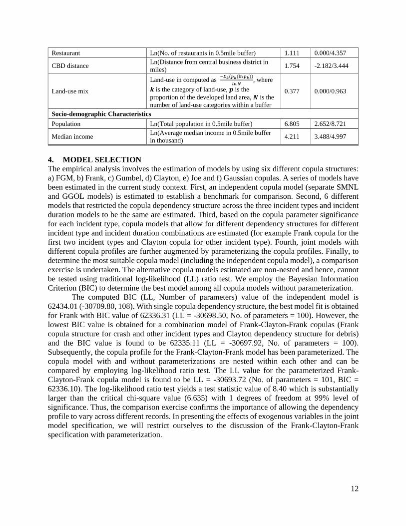
5.2.8 Variance Components

As described in the methodology section, the variance of the GGOL model components are

estimated as a function of observed exogenous variables. The parameter estimates of these

components are presented in the third-row panel of Table 3. From the results, it can be found that

the exogenous variables that contribute to the variance profile of duration model of crash

incidences include notified agency is Road Rangers and number of responders. The only

exogenous variable that contributes to the variance profile of duration model of debris is outside

shoulder width. The exogenous variables that contribute to the variance profile of duration model

of other incidents include AADT, at intersection, first responder is Road Rangers and the incident

was notified to Road Rangers. Thus, these results highlight the presence of heteroscedasticity in

the data.

5.2.9 Dependence Effects

As indicated earlier, the estimated Frank-Clayton-Frank copula based SMNL-GGOL model with

parameterization provides the best fit in incorporating the correlation between incident type and

incident duration. The result of the dependency profile is presented in the last row panel of Table

3. The results clearly highlight the presence of common unobserved factors affecting incident type

and incident duration. The Frank copula dependency structure is associated with the crash and

other incident categories, while the Clayton dependency structure is associated with the debris

category. For the crash incident type, the Frank dependency is negative indicating that the

unobserved factors that are likely to increase crash likelihood are likely to reduce the incident

duration. The Frank dependency for other incidents offers similar results. The reader would note

that for other incident type, the dependency parameter varies by season. Finally, for debris

incident, Clayton copula parameter indicates that the unobserved factors affecting debris incident

and its associated duration have a strong lower tail dependency.

TABLE 3 Parameter Estimates for Incident Duration

Variables Crash Debris Other Incidents

Est. t-stat Est. t-stat Est. t-stat

Propensity components

Constant 104.2761 12.9790 -12.6649 -0.6340 78.3892 4.5180

Incident characteristics

No. of responders 9.7250 10.0730 24.5795 4.4010 25.9121 4.4290

First responder (Base: Other agencies)

Road Ranger -9.2166 -4.6170 -27.5312 -4.7480 -37.0589 -4.0290

Notified agency (Base: Other agencies)

Road Ranger --1 -- -36.8587 -6.4270 -49.5242 -8.0620


Functional class (Base: Other classes)

Rural arterial -- -- 13.2396 2.8060 -102.6595 -9.5910

Urban freeway -- -- -- -- -27.8564 -4.4550

Traffic characteristics


18

6am – 9am -11.1390 -3.8540 -24.2698 -3.2280 14.5904 2.2610

9am – 4pm -10.7558 -4.6140 -21.5290 -3.0470 -40.7983 -7.3300

4pm – 6pm -5.8756 -2.1250 -25.9414 -3.4110 -36.9026 -5.6730

6pm – 9pm -7.8879 -2.8990 -20.1242 -2.7090 -22.5256 -3.5450


Weekday -3.9172 -2.0310 6.0762 2.1960 -- --

Weather condition

Season (Base: Other Seasons)

Summer -- -- 5.4717 2.1250 -- --

Built Environment

CBD distance 4.0977 3.7370 -- -- -- --


Population -5.2669 -5.7490 -- -- -6.7246 -4.0450

Median income -- -- -8.2901 -2.1660 -- --

Category-specific constants

Constant for T1 19.7306 7.3080 14.6056 9.6070 122.1130 27.4130

Constant for T2 8.7898 5.5190 -- -- 73.8363 23.8800

Constant for T3 -- -- -- -- 40.8383 19.5830

Constant for T4 -- -- -- -- 16.4859 13.5050

Constant for T5 -- -- -- -- -- --

Constant for T6 -- -- -- -- -- --

Constant for T7 -- -- -- -- -- --

Constant for T8 -- -- -- -- -- --

Constant for T9 18.8899 14.1380 24.0710 7.2220 -- --

Variance components

Constant 3.3264 57.6220 3.2171 42.1950 3.8284 53.9040

No. of responders -0.1324 -5.5390 -- -- -- --


Road Ranger -- -- -- -- 0.5878 8.4000


Road Ranger 0.4490 6.4160 -- -- -0.0711 -2.3800

At intersection or not (Base: Non-intersection)

At intersection -- -- -- -- 0.1458 2.8510

AADT -- -- -- -- 0.0323 2.1030

Outside shoulder -- -- 0.0594 2.1690 -- --

Dependence Effects

Constant -2.5268 -4.5610 4.8241 4.4080 -1.5917 -3.7590

Season (Base: Other seasons)

Summer -- -- -- -- -0.8163 -2.8940

19

1-- = Attributes insignificant at 90% confidence level

6 MODEL PERFORMANCE AND APPLICATION

6.1 Validation Analysis

To test the predictive performance of the estimated model, a validation exercise with holdout

sample is performed. For this validation test, 2500 records from each year are drawn randomly

from the unused data resulting in a validation dataset of 15,000 records. For testing the predictive

performance of the models, 25 data samples, of about 1000 records each, are randomly generated

from the hold out validation sample consisting of 15,000 records. The average log-likelihood and

BIC score for the copula model are -3046.67 [(-3089.91, -3003.44)] and 6792.93 [(6705.32,

6880.54)], respectively. The average log-likelihood and BIC score for the independent model are

-3050.62 [(-3092.55, -3008.69)], and 6849.30 [(6764.22 ,6934.38)], respectively. The average log-

likelihood and BIC score for the traditional model (single duration model using incident type as

an independent variable) are -3150.97 [(-3193.39, -3108.55)], and 6800.64 [(6714.99, 6886.30)],

respectively. For every individual sample, the predicted log-likelihood and BIC value for the

copula model are better than the corresponding log-likelihood and BIC value for the independent

and the traditional model. The validation result clearly reflects the superiority of joint model over

independent and traditional model.

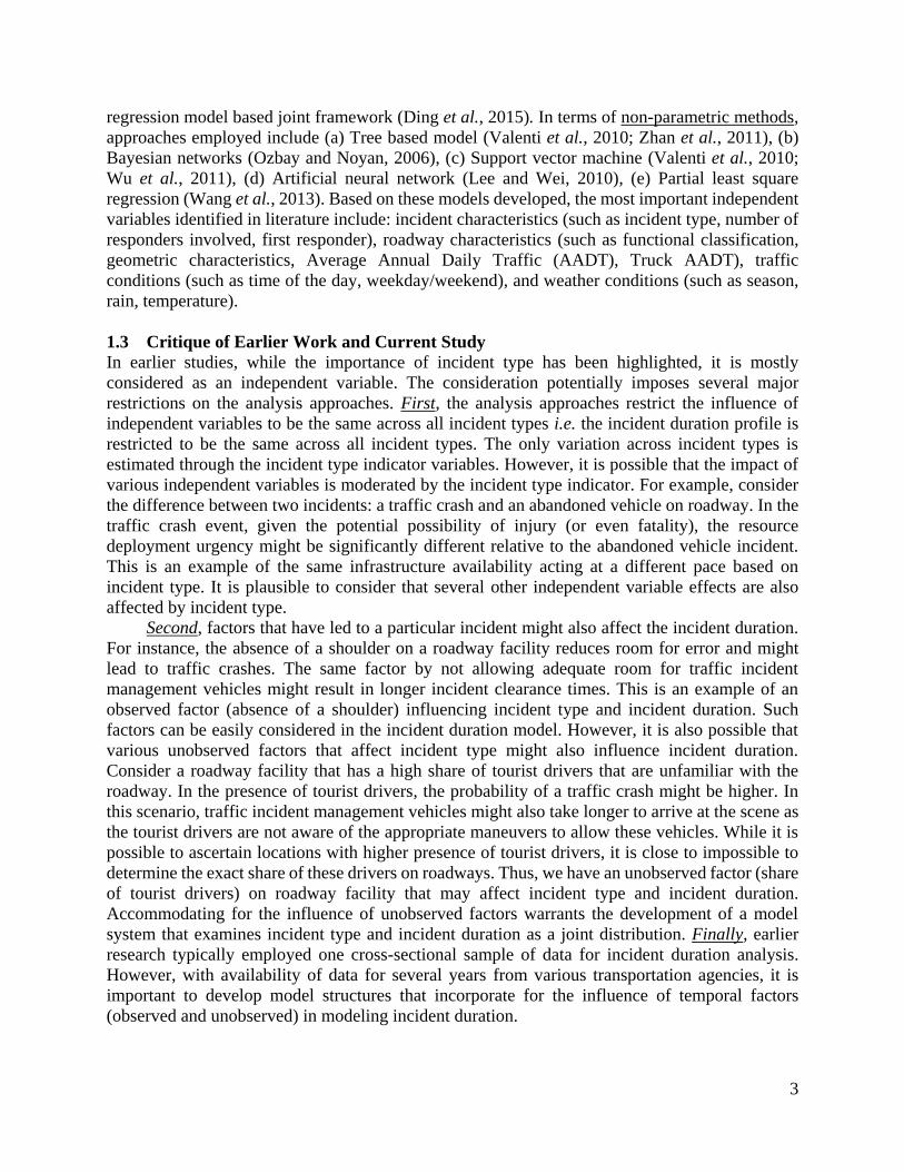
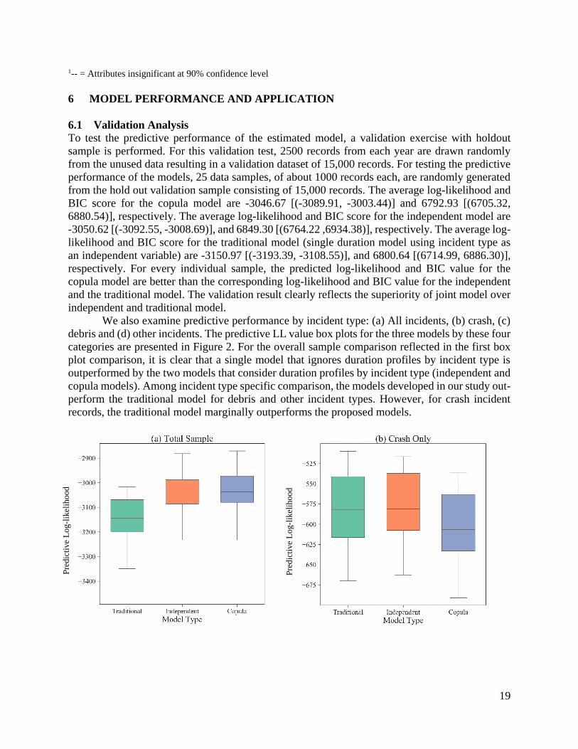
We also examine predictive performance by incident type: (a) All incidents, (b) crash, (c)

debris and (d) other incidents. The predictive LL value box plots for the three models by these four

categories are presented in Figure 2. For the overall sample comparison reflected in the first box

plot comparison, it is clear that a single model that ignores duration profiles by incident type is

outperformed by the two models that consider duration profiles by incident type (independent and

copula models). Among incident type specific comparison, the models developed in our study out-

perform the traditional model for debris and other incident types. However, for crash incident

records, the traditional model marginally outperforms the proposed models.

Pre

dic

tive

Log

-lik

elih

ood

Pre

dic

tive

Log-l

ikel

iho

od

20

FIGURE 2 Comparison of Predictive Log-likelihood of the Three Models

6.2 Elasticity Analysis

The parameter estimates of developed copula-based incident model can be utilized to identify

whether an independent variable increases or decreases the probability of higher/lower order

incident duration categories. But parameter estimates do not directly identify the magnitude of the

change on the probability of a duration category. Therefore, elasticity effects for all independent

variables with regard to incident duration were calculated. For the sake of brevity, we restrict

ourselves to the presentation of elasticity values of the highest duration category in Table 4. Values

presented in Table 4 reflect the percentage change in aggregate probability of the highest duration

category due to the change in independent variables. From the elasticity analysis results, it is found

that an increase in the number of responders increases the probability of higher ordered incident

duration categories significantly. On the other hand, Road rangers being the first responder and

the incident being notified by the Road Rangers reduce the probability of higher ordered duration

categories. In case of traffic characteristics variables, crashes and debris occurring 6am to 9pm

and other incidents occurring 9am to 9pm have lower duration compared to nighttime from 9am

to 6am. With increasing CBD distance, duration of crashes increases significantly. With increased

population in close proximity of crashes and other incidents, incident duration decreases

significantly. Another socio-demographic characteristic, median income significantly influences

duration of debris type of incident. Increase of median income decreases the probability of higher

order duration category. Overall, the elasticity analysis results can be helpful to the incident

management agencies to identify the dominant factors affecting incident duration.

Pre

dic

tive

Log

-lik

elih

ood

Pre

dic

tive

Log

-lik

elih

ood

21

TABLE 4 Elasticity Analysis for Incident Duration

Variables Crash Debris Other Incidents

Incident characteristics

No. of responders 3.06799 6.83959 0.84843


Road Ranger -14.82945 -104.78980 -4.92734


Road Ranger 0.26746 -65.26592 -16.50839


Functional class (Base: Other classes)

Rural arterial -- 41.09485 -23.75875

Urban freeway -- -- -8.087557

Traffic characteristics


6am – 9am -17.55639 -56.43968 4.531904

9am – 4pm -16.94333 -61.75876 -12.17580

4pm – 6pm -9.287986 -55.22964 -10.54608

6pm – 9pm -12.47041 -43.79461 -6.61213


Weekday -6.18817 15.51287 --

Weather condition

Season (Base: Other Seasons)

Summer -- 14.96467 --

Built Environment

CBD distance 4.10584 -- --


Population -5.64136 -- -1.37324

Median income -- -8.72836 --

* Values indicate the percentage changes of aggregated probability of the highest duration category

6.3 Model Illustration

To demonstrate the applicability of the developed model, the final model was applied to generate

response surface using duration categories, incident frequencies and selected independent

variables for different incident types. In generating the values for plotting the response surface, the

incident duration categories are identified based on probabilistic assignment by using predicted

probabilities computed from the final copula model (Frank-Clayton-Frank parameterized). The

probabilities are appropriately aggregated across categories to identify the corresponding incident

frequencies. For example, incident frequencies of crashes are plotted against duration categories

and number of responders in Figure 3a. The plotted surface shows that crash incidents are typically

associated with longer clearance times and are likely to involve increased number of responders

compared to other incident types. Figure 3b presents crash incident frequencies by time of the day

and indicates that crash frequency is the highest between 9am to 4pm compared to other time of

the day. Similar to Figure 3a, crash incident frequencies are higher for longer duration levels.

22

Figure 3c indicates that the likelihood of crash incidents is higher for locations between 5 to 10

miles from central business district. Figure 3d presents other incident frequencies by duration

category and time of the day. The reader would note that the plots provided are only a sample of

the various illustrations that can be generated based on the independent variables in the models.

The development of such response surface could be helpful for the incident management agencies

to allocate their resources based on the reported incident scenarios.

23

(a) Crash frequencies with respect to number of responders (b) Crash frequencies with respect to time of the day

(c) Crash frequencies with respect to CBD distance (d) Other Incidents frequencies with respect to time of the day

FIGURE 3 Response Surface for Predicted Incident Frequencies

12

34

5

0

200

400

600

800

Fre

quen

cy

0-200 200-400 400-600 600-800

6am-9am9am-4pm

4pm-6pm6pm-9pm

9pm-6am

0

100

200

300

400

500

Fre

quen

cy

0-100 100-200 200-300 300-400 400-500

6am-9am

0-5>5-10

>10-15

>15

0

200

400

600

800

Fre

quen

cy

0-200 200-400 400-600 600-800

0-5 6am-9am9am-4pm

4pm-6pm6pm-9pm

9pm-6am

0

500

1000

1500

Fre

quen

cy

0-500 500-1000 1000-1500

6am-9am

1

24

7 CONCLUSION

To understand the impact of observed and unobserved effects on incident type and incident

duration, this paper formulated and estimated a copula-based joint model with a scaled

multinomial logit model (SMNL) system for incident type and a grouped generalized ordered logit

(GGOL) model system for incident duration. The proposed model is estimated using FDOT’s

incident management data from Greater Orlando region, with a host of independent variables

including incident characteristics, roadway characteristics, traffic condition, weather condition,

built environment and socio-demographic characteristics. The current study contributes to incident

duration literature in multiple ways. First, the current study posits that incident duration is strongly

influenced by incident type and allows for distinct incident profile regimes. Further, the study

accommodates for common unobserved factors affecting incident type and incident type within a

closed form copula-based model structure. Second, the study using data from multiple years,

develops a framework that accommodates for observed and unobserved temporal effects on

incident type and incident duration. Finally, the proposed model system is estimated using a

comprehensive set of exogenous variables.

The empirical analysis involves the estimation of models by using six different copula

structures: 1) FGM, 2) Clayton, 3) Gumbel, 4) Frank, 5) Joe and 6) Gaussian. The parameterized

Frank-Clayton-Frank copula system (Frank copula structure for crash and other incident type and

Clayton dependency structure for debris) offered the best data fit for our empirical context. The

model estimation results presented in the current paper suggest that the impact of exogenous

variables vary (for some variables) in magnitude as well as in sign across incident types. To further

understand the performance of the developed model, a comprehensive model performance

evaluation and applicability exercise was conducted. The results from the exercise illustrate the

value offered by the proposed model system.

The enhanced duration model can be employed by planning agencies to guide incident

clearance as well as traffic congestion management. To elaborate, based on the model system,

planning agencies can generate guidelines on incident duration times for important variables such

as incident type, location and time of day. These guideline durations for incident clearance can

allow agencies to identify the appropriate messaging signs (such as what is targeted demand for

diversion) for route detours at the occurrence of an incident.

ACKNOWLEDGEMENT

The authors would like to acknowledge Florida Department of Transportation to provide access to

their incident management dataset.

AUTHOR CONTRIBUTION STATEMENT

The authors confirm contribution to the paper as follows: study conception and design: Naveen

Eluru, Shamsunnahar Yasmin, Sudipta Dey Tirtha; data collection: Sudipta Dey Tirtha,

Shamsunnahar Yasmin, Naveen Eluru; model estimation: Sudipta Dey Tirtha, Shamsunnahar

Yasmin, Naveen Eluru; analysis and interpretation of results: Sudipta Dey Tirtha, Naveen Eluru,

Shamsunnahar Yasmin; draft manuscript preparation: Sudipta Dey Tirtha, Naveen Eluru,

Shamsunnahar Yasmin. All authors reviewed the results and approved the final version of the

manuscript.

25

REFERENCES

Anowar, S., Eluru, N., & Miranda-Moreno, L. F. (2016). ‘Analysis of vehicle ownership evolution

in Montreal, Canada using pseudo panel analysis’. Transportation, 43(3), 531-548.

Behnood, A., & Mannering, F. L. (2015). ‘The temporal stability of factors affecting driver-injury

severities in single-vehicle crashes: some empirical evidence’. Analytic methods in

accident research, 8, 7-32.

Bhat, C. R. and Eluru, N. (2009) ‘A copula-based approach to accommodate residential self-

selection effects in travel behavior modeling’, Transportation Research Part B:

Methodological. Elsevier Ltd, 43(7), pp. 749–765. doi: 10.1016/j.trb.2009.02.001.

Chung, Y. (2010) ‘Development of an accident duration prediction model on the Korean Freeway

Systems’, Accident Analysis and Prevention, 42(1), pp. 282–289. doi:

10.1016/j.aap.2009.08.005.

Chung, Y. S., Chiou, Y. C. and Lin, C. H. (2015) ‘Simultaneous equation modeling of freeway

accident duration and lanes blocked’, Analytic Methods in Accident Research. Elsevier, 7,

pp. 16–28. doi: 10.1016/j.amar.2015.04.003.

Dabbour, E. (2017). ‘Investigating temporal trends in the explanatory variables related to the

severity of drivers' injuries in single-vehicle collisions’. Journal of traffic and

transportation engineering (English edition), 4(1), 71-79.

Ding, C., Ma, X., Wang, Y. and Wang, Y. (2015) ‘Exploring the influential factors in incident

clearance time: Disentangling causation from self-selection bias’, Accident Analysis and

Prevention. Elsevier Ltd, 85, pp. 58–65. doi: 10.1016/j.aap.2015.08.024.

FHWA EDC (2012) ‘SHRP2 Traffic Incident Management Responder Training’. Available at:

http://www.fhwa.dot.gov/everydaycounts/edctwo/2012/pdfs/edc_traffic.pdf.

Garib, A., Radwan, A. E. and Al-Deek, H. (2002) ‘Estimating Magnitude and Duration of Incident

Delays’, Journal of Transportation Engineering, 123(6), pp. 459–466. doi:

10.1061/(asce)0733-947x(1997)123:6(459).

Ghosh, I., Savolainen, P. T. and Gates, T. J. (2014) ‘Examination of factors affecting freeway

incident clearance times: A comparison of the generalized F model and several alternative

nested models’, Journal of Advanced Transportation, 48(6), pp. 471–485. doi:

10.1002/atr.1189.

HCM 2010 : highway capacity manual (no date). Fifth edition. Washington, D.C. : Transportation

Research Board, c2010-. Available at:

https://search.library.wisc.edu/catalog/9910110589002121.

INRIX (2018) No Title. Available at: http://inrix.com/scorecard/.

Junhua, W., Haozhe, C. and Shi, Q. (2013) ‘Estimating freeway incident duration using accelerated

failure time modeling’, Safety Science. Elsevier Ltd, 54, pp. 43–50. doi:

10.1016/j.ssci.2012.11.009.

Khattak, A. J., Schofer, J. L. and Wang, M.-H. (2007) ‘A Simple Time Sequential Procedure for

Predicting Freeway Incident Duration’, I V H S Journal, 2(2), pp. 113–138. doi:

10.1080/10248079508903820.

Laman, H., Yasmin, S. and Eluru, N. (2018) ‘Joint modeling of traffic incident duration

components (reporting, response, and clearance time): A copula-based approach’,

Transportation Research Record, 2672(30), pp. 76–89. doi: 10.1177/0361198118801355.

Lee, Y. and Wei, C. H. (2010) ‘A computerized feature selection method using genetic algorithms

to forecast freeway accident duration times’, Computer-Aided Civil and Infrastructure

Engineering, 25(2), pp. 132–148. doi: 10.1111/j.1467-8667.2009.00626.x.

26

Li, R., Pereira, F. C. and Ben-Akiva, M. E. (2015) ‘Competing risk mixture model and text analysis

for sequential incident duration prediction’, Transportation Research Part C: Emerging

Technologies. Elsevier Ltd, 54, pp. 74–85. doi: 10.1016/j.trc.2015.03.009.

Mannering, F. (2018). ‘Temporal instability and the analysis of highway accident data’. Analytic

methods in accident research, 17, 1-13.

Marcoux, R., Yasmin, S., Eluru, N., & Rahman, M. (2018). ‘Evaluating temporal variability of

exogenous variable impacts over 25 years: An application of scaled generalized ordered

logit model for driver injury severity’. Analytic methods in accident research, 20, 15-29.

Ozbay, K. and Noyan, N. (2006) ‘Estimation of incident clearance times using Bayesian Networks

approach’, Accident Analysis and Prevention, 38(3), pp. 542–555. doi:

10.1016/j.aap.2005.11.012.

Sklar, A. (1973) ‘Random variables, joint distribution functions, and copulas’, Kybernetika, 9(6),

pp. 449–460.

Tavassoli Hojati, A., Ferreira, L., Washington, S. and Charles, P. (2013) ‘Hazard based models for

freeway traffic incident duration’, Accident Analysis and Prevention. Elsevier Ltd, 52, pp.

171–181. doi: 10.1016/j.aap.2012.12.037.

Tavassoli Hojati, A., Ferreira, L., Washington, S., Charles, P. and Shobeirinejad, A. (2014)

‘Modelling total duration of traffic incidents including incident detection and recovery

time’, Accident Analysis and Prevention. Elsevier Ltd, 71, pp. 296–305. doi:

10.1016/j.aap.2014.06.006.

Valenti, G., Lelli, M. and Cucina, D. (2010) ‘A comparative study of models for the incident

duration prediction’, European Transport Research Review, 2(2), pp. 103–111. doi:

10.1007/s12544-010-0031-4.

Wang, X., Chen, S. and Zheng, W. (2013) ‘Traffic Incident Duration Prediction based on Partial

Least Squares Regression’, Procedia - Social and Behavioral Sciences. Elsevier B.V.,

96(Cictp), pp. 425–432. doi: 10.1016/j.sbspro.2013.08.050.

Wu, W., Chen, S. and Zheng, C. (2011) ‘Traffic Incident Duration Prediction Based on Support

Vector Regression’, pp. 2412–2421. doi: 10.1061/41186(421)241.

Zhan, C., Gan, A. and Hadi, M. (2011) ‘Prediction of lane clearance time of freeway incidents

using the M5P tree algorithm’, IEEE Transactions on Intelligent Transportation Systems.

IEEE, 12(4), pp. 1549–1557. doi: 10.1109/TITS.2011.2161634.

Documents

Modeling of Incident Type and Incident Duration Using Data