Modeling of Highly Instrumented Honeywell Turbofan Engine ...Modeling of Highly Instrumented Honeywell Turbofan Engine Tested with Ice Crystal Ingestion in the NASA Propulsion System

American Institute of Aeronautics and Astronautics

1

Modeling of Highly Instrumented Honeywell Turbofan

Engine Tested with Ice Crystal Ingestion in the NASA

Propulsion System Laboratory

Joseph P. Veres1, Philip C. E. Jorgenson2, Scott M. Jones3

The Propulsion Systems Laboratory (PSL), an altitude test facility at NASA Glenn

Research Center, has been used to test a highly instrumented turbine engine at simulated

altitude operating conditions. This is a continuation of the PSL testing that successfully

duplicated the icing events that were experienced in a previous engine (serial LF01) during flight

through ice crystal clouds, which was the first turbofan engine tested in PSL. This second model

of the ALF502R-5A serial number LF11 is a highly instrumented version of the previous engine.

The PSL facility provides a continuous cloud of ice crystals with controlled characteristics of

size and concentration, which are ingested by the engine during operation at simulated altitudes.

Several of the previous operating points tested in the LF01 engine were duplicated to confirm

repeatability in LF11. The instrumentation included video cameras to visually illustrate the

accretion of ice in the low pressure compressor (LPC) exit guide vane region in order to confirm

the ice accretion, which was suspected during the testing of the LF01. Traditional

instrumentation included static pressure taps in the low pressure compressor inner and outer

flow path walls, as well as total pressure and temperature rakes in the low pressure compressor

region. The test data was utilized to determine the losses and blockages due to accretion in the

exit guide vane region of the LPC. Multiple data points were analyzed with the Honeywell

Customer Deck. A full engine roll back point was modeled with the Numerical Propulsion

System Simulation (NPSS) code. The mean line compressor flow analysis code with ice crystal

modeling was utilized to estimate the parameters that indicate the risk of accretion, as well as

to estimate the degree of blockage and losses caused by accretion during a full engine roll back

point. The analysis provided additional validation of the icing risk parameters within the LPC,

as well as the creation of models for estimating the rates of blockage growth and losses.

1 Aerospace Engineer, Lead, Engine Icing Technical Challenge, Turbomachinery and Heat Transfer Branch, NASA

Glenn Research Center, 21000 Brookpark Rd. Cleveland, Ohio 44135/Mail Stop 5-11 2 Aerospace Engineer, Turbomachinery and Heat Transfer Branch, NASA Glenn Research Center, 21000 Brookpark

Rd. Cleveland, Ohio 44135/Mail Stop 5-11 3 Aerospace Engineer, Propulsion Systems Analysis Branch, NASA Glenn Research Center, 21000 Brookpark Rd.

Cleveland, Ohio 44135/Mail Stop 5-11

https://ntrs.nasa.gov/search.jsp?R=20170000246 2020-04-23T17:16:10+00:00Z


2

Introduction

HE highly instrumented turbine engine ALF502R-5A serial LF11 (Figure 1) has been tested in the Propulsion

Systems Laboratory (PSL), an altitude test facility at NASA Glenn Research Center. The PSL facility provides a

continuous cloud of ice crystals with controlled characteristics of size and concentration, which are ingested by the

engine during operation at simulated altitudes. The purpose of the PSL testing is to improve understanding of the

turbofan engine icing events1,2 that have occurred in the turbofan engines of commercial airlines during flight through

clouds with high ice water content. These events have been attributed to ice crystal ingestion and subsequent ice

accretion in the compression system of the engine, which is responsible for the uncommanded loss of thrust (roll

back). Testing of the LF11 engine is a continuation of the testing that was performed in 2013 on a similar engine

(ALF502R-5A serial LF01)3,4,5.

This second model of the ALF502R-5A engine is a highly instrumented version of the previous engine. Several of the

previous operating points tested in the LF01 engine were duplicated to confirm repeatability in the LF11. The

instrumentation included video cameras to visually confirm the accretion of ice in the low pressure compressor (LPC)

exit guide vane region, which was suspected during the testing of the LF01. Traditional instrumentation included wall

static pressure taps as well as total pressure and temperature rakes in the low pressure compressor, exit guide vane and

goose neck regions. Fifty-five Escort test data points were analyzed with the Honeywell Customer Deck (CD) and

with a mean-line compressor flow code to estimate the values of key parameters that indicate the risk of accretion. Of

those, twenty-two test data points were selected to highlight “threshold points” where the engine reached a partially

degraded yet stable operating state, and the fastest roll back points which indicated that a roll back would be imminent

(Appendix A). In addition, one full engine roll back point was modeled with the Numerical Propulsion System

Simulation (NPSS) code to estimate the performance degradation of the LPC due to accretion. The NPSS6,7 model of

the LPC provided the boundary conditions for the mean-line compressor flow model (COMDES)8,9 These two codes

comprise the mixed fidelity computational tool that was utilized to provide details of the flow conditions within each

blade row of the fan and low pressure compression system (LPC) during operation in the engine system environment.

a) b)

Figure 1: a) ALF502R-5A Turbofan Engine. b) The enlargement of the fan and single-stage LPC illustrating

the IGV and the tandem stator; EGV stator 1 and EGV stator 2.

Ice accretion in the LPC is a transient phenomenon and reduces the available aerodynamic area and deteriorates the

performance of the compressor component where the accretion takes place, and consequently effects the overall

performance of the engine. Modeling the full roll back data point at discreet Escort scan numbers with the mean-line

compressor code required manually modifying the blockages and losses at the stator leading and trailing edges in the

IGV and the tandem stator (EGV stator 1 and EGV stator 2). At each Escort scan number analyzed, the NPSS model

results for pressure ratio and efficiency were utilized as boundary conditions for the compressor flow analysis.

Additional losses in the IGV and EGV were required in the compressor as well as additional blockages were required

T


3

in the compressor flow model to match the measured static pressure at the flow path walls near the leading and trailing

edges.

I. Quantify Key Parameters Associated with Ice Accretion Risk

The first phase of this study involved the analysis of the select Escort data points in order to determine the values of

key icing parameters associated with ice accretion, which for this small turbofan engine, could lead to engine roll

back. The select test data points analyzed included both engine roll back and non roll back data points at a range of

simulated altitudes. Note that for these roll back points the test engineer made the determination that the engine roll

back would have been imminent. The imminent roll back was called in order to prevent possible damage due to ice

shedding and impacting the high pressure compressor blades. For this reason, only one full engine roll back test point

was conducted (Escort data point 093), which will be discussed in a subsequent section.

A. Aerothermodynamic Simulation of the Engine System; Customer Deck and Compressor Flow Model

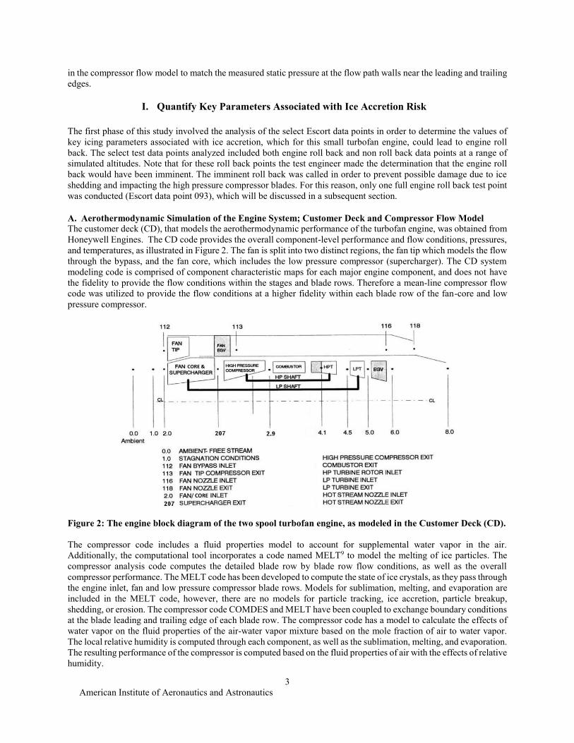
The customer deck (CD), that models the aerothermodynamic performance of the turbofan engine, was obtained from

Honeywell Engines. The CD code provides the overall component-level performance and flow conditions, pressures,

and temperatures, as illustrated in Figure 2. The fan is split into two distinct regions, the fan tip which models the flow

through the bypass, and the fan core, which includes the low pressure compressor (supercharger). The CD system

modeling code is comprised of component characteristic maps for each major engine component, and does not have

the fidelity to provide the flow conditions within the stages and blade rows. Therefore a mean-line compressor flow

code was utilized to provide the flow conditions at a higher fidelity within each blade row of the fan-core and low

pressure compressor.

Figure 2: The engine block diagram of the two spool turbofan engine, as modeled in the Customer Deck (CD).

The compressor code includes a fluid properties model to account for supplemental water vapor in the air.

Additionally, the computational tool incorporates a code named MELT9 to model the melting of ice particles. The

compressor analysis code computes the detailed blade row by blade row flow conditions, as well as the overall

compressor performance. The MELT code has been developed to compute the state of ice crystals, as they pass through

the engine inlet, fan and low pressure compressor blade rows. Models for sublimation, melting, and evaporation are

included in the MELT code, however, there are no models for particle tracking, ice accretion, particle breakup,

shedding, or erosion. The compressor code COMDES and MELT have been coupled to exchange boundary conditions

at the blade leading and trailing edge of each blade row. The compressor code has a model to calculate the effects of

water vapor on the fluid properties of the air-water vapor mixture based on the mole fraction of air to water vapor.

The local relative humidity is computed through each component, as well as the sublimation, melting, and evaporation.

The resulting performance of the compressor is computed based on the fluid properties of air with the effects of relative

humidity.


4

The inputs provided to the CD system modeling code are the altitude, flight Mach number, fan physical rotational

speed, and the air static temperature. The model results include the aerothermodynamic performance of each major

engine component, as described in Figure 2, including the bypass ratio. The main purpose of the CD engine system

model was to provide the bypass ratio and thus, the air mass flow into the engine core.

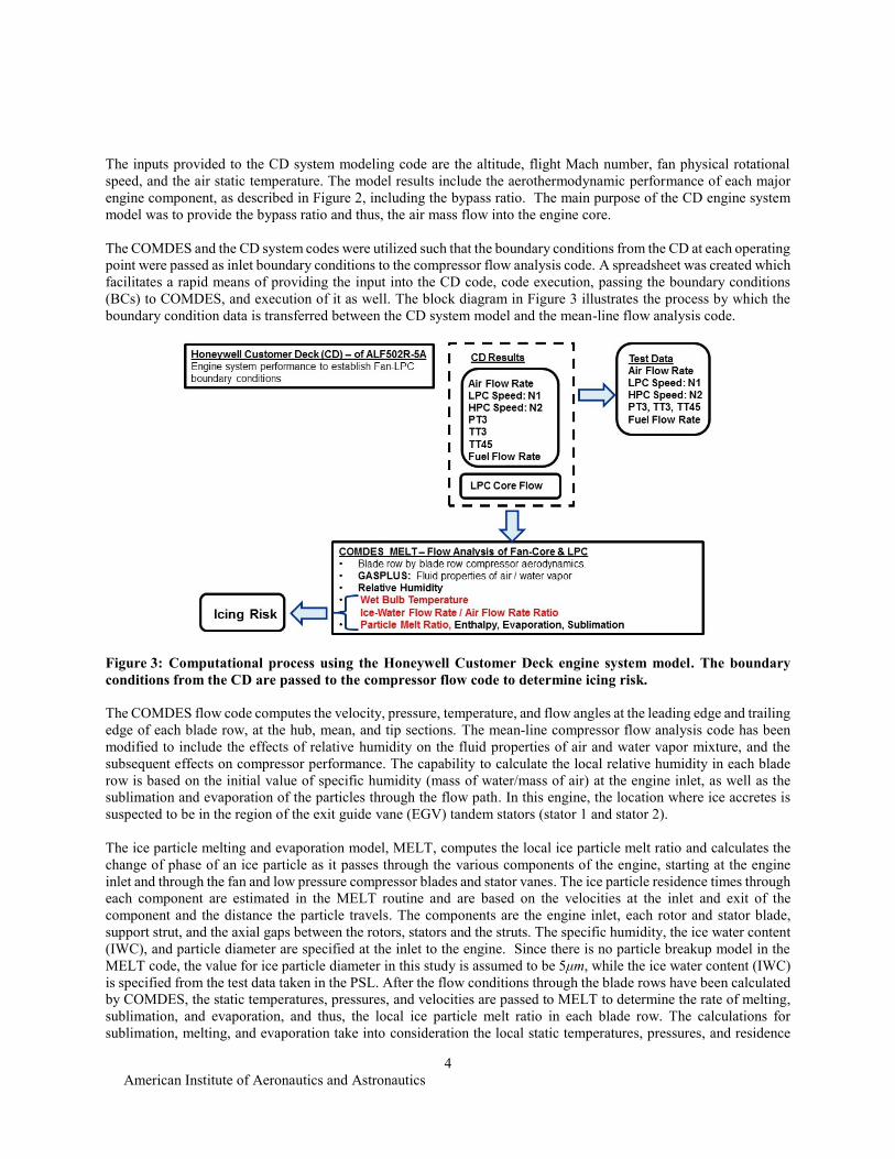
The COMDES and the CD system codes were utilized such that the boundary conditions from the CD at each operating

point were passed as inlet boundary conditions to the compressor flow analysis code. A spreadsheet was created which

facilitates a rapid means of providing the input into the CD code, code execution, passing the boundary conditions

(BCs) to COMDES, and execution of it as well. The block diagram in Figure 3 illustrates the process by which the

boundary condition data is transferred between the CD system model and the mean-line flow analysis code.

Figure 3: Computational process using the Honeywell Customer Deck engine system model. The boundary

conditions from the CD are passed to the compressor flow code to determine icing risk.

The COMDES flow code computes the velocity, pressure, temperature, and flow angles at the leading edge and trailing

edge of each blade row, at the hub, mean, and tip sections. The mean-line compressor flow analysis code has been

modified to include the effects of relative humidity on the fluid properties of air and water vapor mixture, and the

subsequent effects on compressor performance. The capability to calculate the local relative humidity in each blade

row is based on the initial value of specific humidity (mass of water/mass of air) at the engine inlet, as well as the

sublimation and evaporation of the particles through the flow path. In this engine, the location where ice accretes is

suspected to be in the region of the exit guide vane (EGV) tandem stators (stator 1 and stator 2).

The ice particle melting and evaporation model, MELT, computes the local ice particle melt ratio and calculates the

change of phase of an ice particle as it passes through the various components of the engine, starting at the engine

inlet and through the fan and low pressure compressor blades and stator vanes. The ice particle residence times through

each component are estimated in the MELT routine and are based on the velocities at the inlet and exit of the

component and the distance the particle travels. The components are the engine inlet, each rotor and stator blade,

support strut, and the axial gaps between the rotors, stators and the struts. The specific humidity, the ice water content

(IWC), and particle diameter are specified at the inlet to the engine. Since there is no particle breakup model in the

MELT code, the value for ice particle diameter in this study is assumed to be 5μm, while the ice water content (IWC)

is specified from the test data taken in the PSL. After the flow conditions through the blade rows have been calculated

by COMDES, the static temperatures, pressures, and velocities are passed to MELT to determine the rate of melting,

sublimation, and evaporation, and thus, the local ice particle melt ratio in each blade row. The calculations for

sublimation, melting, and evaporation take into consideration the local static temperatures, pressures, and residence


5

times as they traverse through the engine inlet, the fan-core and low pressure compressor blade passages and gaps at

the mid-span location, the gooseneck duct and the support strut. This requires an iterative exchange of boundary

conditions between the COMDES and MELT codes as there is a change in fluid properties of the air as well as an

exchange of enthalpy between the ice and the air.

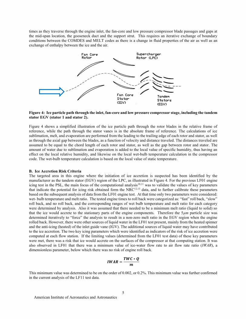
Figure 4: Ice particle path through the inlet, fan-core and low pressure compressor stage, including the tandem

stator EGV (stator 1 and stator 2).

Figure 4 shows a simplified illustration of the ice particle path through the rotor blades in the relative frame of

reference, while the path through the stator vanes is in the absolute frame of reference. The calculations of ice

sublimation, melt, and evaporation are performed from the leading to the trailing edge of each rotor and stator, as well

as through the axial gap between the blades, as a function of velocity and distance traveled. The distances traveled are

assumed to be equal to the chord length of each rotor and stator, as well as the gap between rotor and stator. The

amount of water due to sublimation and evaporation is added to the local value of specific humidity, thus having an

effect on the local relative humidity, and likewise on the local wet-bulb temperature calculation in the compressor

code. The wet-bulb temperature calculation is based on the local value of static temperature.

B. Ice Accretion Risk Criteria

The targeted area in this engine where the initiation of ice accretion is suspected has been identified by the

manufacturer as the tandem stator (EGV) region of the LPC, as illustrated in Figure 4. For the previous LF01 engine

icing test in the PSL, the main focus of the computational analysis10,11 was to validate the values of key parameters

that indicate the potential for icing risk obtained form the NRC12,13 data, and to further calibrate these parameters

based on the subsequent analysis of data from the LF01 engine test. At that time only two parameters were considered:

wet- bulb temperature and melt ratio. The tested engine times to roll back were categorized as: “fast” roll back, “slow”

roll back, and no roll back, and the corresponding ranges of wet bulb temperature and melt ratio for each category

were determined by analysis. Also it was assumed that there needed to be a minimum melt ratio (liquid to solid) so

that the ice would accrete to the stationary parts of the engine components. Therefore the 5µm particle size was

determined iteratively to “force” the analysis to result in a non-zero melt ratio in the EGV region when the engine

rolled back. However, there were other sources of liquid water in the LF01 test present, mainly from the heated spinner

and the anti-icing (heated) of the inlet guide vane (IGV). The additional sources of liquid water may have contributed

to the ice accretion. The two key icing parameters which were identified as indicators of the risk of ice accretion were

computed at each flow station. If the limiting values (determined from the LF01 test data) of these key parameters

were met, there was a risk that ice would accrete on the surfaces of the compressor at that computing station. It was

also observed in LF01 that there was a minimum value of ice-water flow rate to air flow rate ratio (IWAR), a

dimensionless parameter, below which there was no risk of engine roll back.

𝑰𝑾𝑨𝑹 =𝑻𝑾𝑪 ∗ 𝑸

𝒎

This minimum value was determined to be on the order of 0.002, or 0.2%. This minimum value was further confirmed

in the current analysis of the LF11 test data.


6

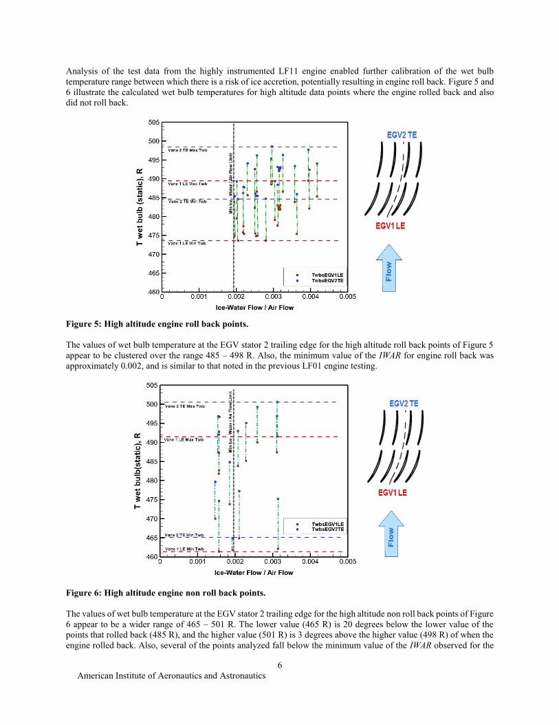
Analysis of the test data from the highly instrumented LF11 engine enabled further calibration of the wet bulb

temperature range between which there is a risk of ice accretion, potentially resulting in engine roll back. Figure 5 and

6 illustrate the calculated wet bulb temperatures for high altitude data points where the engine rolled back and also

did not roll back.

Figure 5: High altitude engine roll back points.

The values of wet bulb temperature at the EGV stator 2 trailing edge for the high altitude roll back points of Figure 5

appear to be clustered over the range 485 – 498 R. Also, the minimum value of the IWAR for engine roll back was

approximately 0.002, and is similar to that noted in the previous LF01 engine testing.

Figure 6: High altitude engine non roll back points.

The values of wet bulb temperature at the EGV stator 2 trailing edge for the high altitude non roll back points of Figure

6 appear to be a wider range of 465 – 501 R. The lower value (465 R) is 20 degrees below the lower value of the

points that rolled back (485 R), and the higher value (501 R) is 3 degrees above the higher value (498 R) of when the

engine rolled back. Also, several of the points analyzed fall below the minimum value of the IWAR observed for the


7

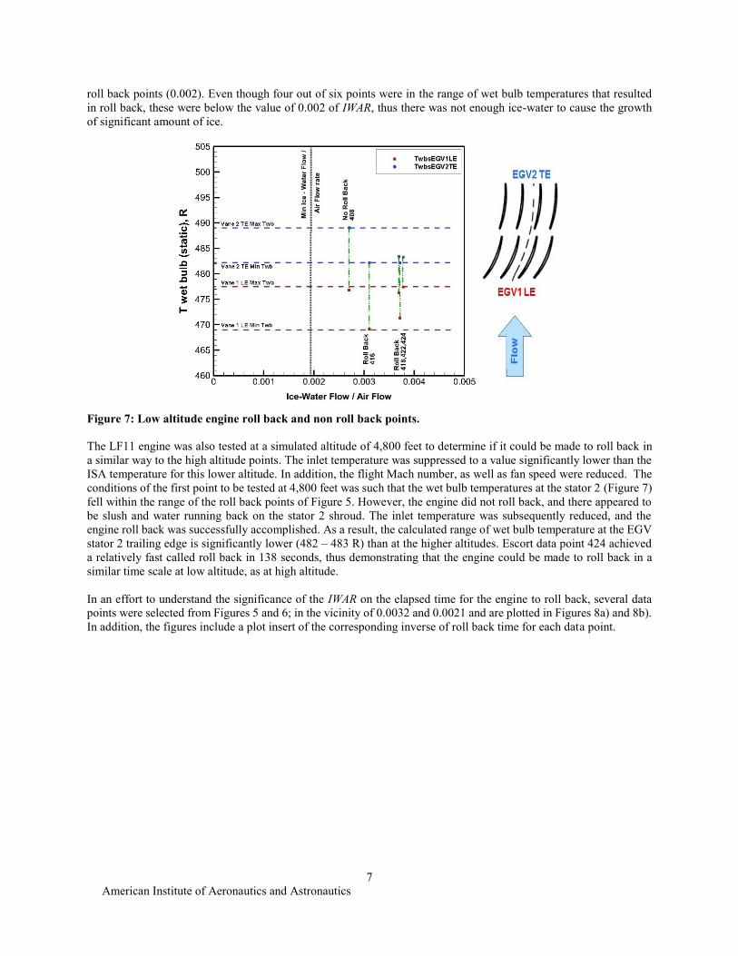
roll back points (0.002). Even though four out of six points were in the range of wet bulb temperatures that resulted

in roll back, these were below the value of 0.002 of IWAR, thus there was not enough ice-water to cause the growth

of significant amount of ice.

Figure 7: Low altitude engine roll back and non roll back points.

The LF11 engine was also tested at a simulated altitude of 4,800 feet to determine if it could be made to roll back in

a similar way to the high altitude points. The inlet temperature was suppressed to a value significantly lower than the

ISA temperature for this lower altitude. In addition, the flight Mach number, as well as fan speed were reduced. The

conditions of the first point to be tested at 4,800 feet was such that the wet bulb temperatures at the stator 2 (Figure 7)

fell within the range of the roll back points of Figure 5. However, the engine did not roll back, and there appeared to

be slush and water running back on the stator 2 shroud. The inlet temperature was subsequently reduced, and the

engine roll back was successfully accomplished. As a result, the calculated range of wet bulb temperature at the EGV

stator 2 trailing edge is significantly lower (482 – 483 R) than at the higher altitudes. Escort data point 424 achieved

a relatively fast called roll back in 138 seconds, thus demonstrating that the engine could be made to roll back in a

similar time scale at low altitude, as at high altitude.

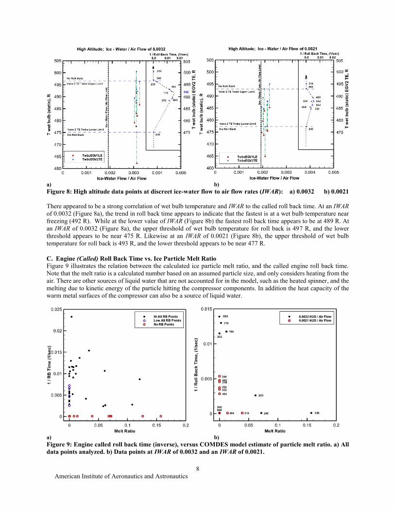
In an effort to understand the significance of the IWAR on the elapsed time for the engine to roll back, several data

points were selected from Figures 5 and 6; in the vicinity of 0.0032 and 0.0021 and are plotted in Figures 8a) and 8b).

In addition, the figures include a plot insert of the corresponding inverse of roll back time for each data point.


8

a) b)

Figure 8: High altitude data points at discreet ice-water flow to air flow rates (IWAR): a) 0.0032 b) 0.0021

There appeared to be a strong correlation of wet bulb temperature and IWAR to the called roll back time. At an IWAR

of 0.0032 (Figure 8a), the trend in roll back time appears to indicate that the fastest is at a wet bulb temperature near

freezing (492 R). While at the lower value of IWAR (Figure 8b) the fastest roll back time appears to be at 489 R. At

an IWAR of 0.0032 (Figure 8a), the upper threshold of wet bulb temperature for roll back is 497 R, and the lower

threshold appears to be near 475 R. Likewise at an IWAR of 0.0021 (Figure 8b), the upper threshold of wet bulb

temperature for roll back is 493 R, and the lower threshold appears to be near 477 R.

C. Engine (Called) Roll Back Time vs. Ice Particle Melt Ratio

Figure 9 illustrates the relation between the calculated ice particle melt ratio, and the called engine roll back time.

Note that the melt ratio is a calculated number based on an assumed particle size, and only considers heating from the

air. There are other sources of liquid water that are not accounted for in the model, such as the heated spinner, and the

melting due to kinetic energy of the particle hitting the compressor components. In addition the heat capacity of the

warm metal surfaces of the compressor can also be a source of liquid water.

a) b)

Figure 9: Engine called roll back time (inverse), versus COMDES model estimate of particle melt ratio. a) All

data points analyzed. b) Data points at IWAR of 0.0032 and an IWAR of 0.0021.


9

The heated IGV is accounted for through the CD engine system model. As illustrated in Figure 9a), there are numerous

data points that had a called engine roll back, even though they had zero particle melt ratio due to heating from the

air. Likewise, there are data points that have a non-zero melt ratio, yet they did not experience an engine roll back.

The reasons for this are that the wet bulb temperature was either too warm to support accretion, or there was not

enough IWAR. Figure 9b) illustrates the called roll back time versus calculated particle melt ratio, for the two specific

values of IWAR (0.0032 and 0.0021). These points are the same as those shown in Figures 8a) and 8b). Note that

neither of the fastest roll back times at the two values of IWAR (Escort data points 093 and 344) show a non-zero

calculated particle melt ratio at the EGV stator 2 trailing edge region. This may indicate that in order for the calculated

melt ratio to be non-zero, the particle size may be even smaller that the assumed 5µm. Concurrently, it may indicate

that heating from the air does not significantly contribute to the liquid water required for accretion to take place.

Alternatively, the other possible sources of liquid water (heated spinner, kinetic energy, heat capacity of the warm

metal surfaces) may be responsible for ice accretion.

D. Engine Roll Back Time vs. Ice-Water Flow to Air Flow Rate (IWAR)

The significance of the IWAR on the elapsed time for the engine to roll back is further illustrated in Figures 10 a) in

which the roll back time versus IWAR is plotted. The peak roll back times are highlighted as the upper limits of roll

back times for IWAR of 0.0032 and 0.0021. The extension of the roll back time limit line beyond 0.005 is based on

Escort data points 160 and 162, which had values of IWAR on the order of 0.007, and called roll back time of 34

seconds.

a) b)

Figure 10: a) Engine roll back time versus IWAR. b) Measured EGV shroud metal temperature (after 20

seconds of ice cloud on) and calculated wet bulb temperatures (before ice cloud) versus IWAR.

Figure 10b) illustrates the shroud metal temperatures at EGV stator 2 trailing edge, 20 seconds after the ice cloud has

been turned on, versus IWAR, at all the roll back points analyzed at all altitudes. It can be seen that there is a

dependence of metal temperature on IWAR. A low value of IWAR below 0.002 cannot cool the metal significantly

enough in order for ice accretion to occur. Concurrently, values of IWAR in the vicinity of 0.003 and greater can

quickly cool the metal temperature to freezing. The calculated wet bulb temperatures at EGV stator 2 trailing edge

prior to ice cloud on condition are also shown for reference in Figure 10b).


10

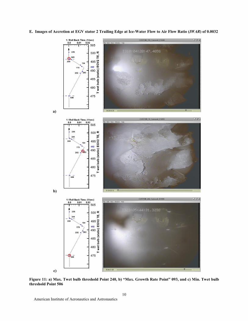
E. Images of Accretion at EGV stator 2 Trailing Edge at Ice-Water Flow to Air Flow Ratio (IWAR) of 0.0032

a)

b)

c)

Figure 11: a) Max. Twet bulb threshold Point 240, b) “Max. Growth Rate Point” 093, and c) Min. Twet bulb

threshold Point 506


11

The images shown in Figure 11 are of three Escort data points at IWAR of 0.0032. Figure 11a) is a no roll back data

point (Escort point 240) that had a high calculated wet bulb temperature (497 R) at EGV stator 2 trailing edge. Even

though the IWAR was acceptably high to support strong accretion in the blade passages, the ice was slushy and there

was ice buildup and shedding taking place. The high value of wet bulb temperature is suspected to be the reason the

ice did not grow at a significant rate over time, and consequently did not roll back. Figure 11b) represents the growth

of ice for Escort data point 093 at Escort scan 72 (47 seconds after the ice cloud was turned on). Note that the wet

bulb temperature at EGV stator 2 trailing edge was near freezing at this data point. There was strong ice accretion

with minimal shedding, and the ice accretion continued to grow, resulting in significant blockage (near 60%) at Escort

scan 305 (discussed later in Section II “Analysis of Full Roll Back Point”). Figure 11c) illustrates the EGV stator 2

trailing edge for Escort data point 506, showing that there was no ice accretion and no roll back occurred. The wet

bulb temperature at this data point was too cold to support ice accretion, at 475 R.

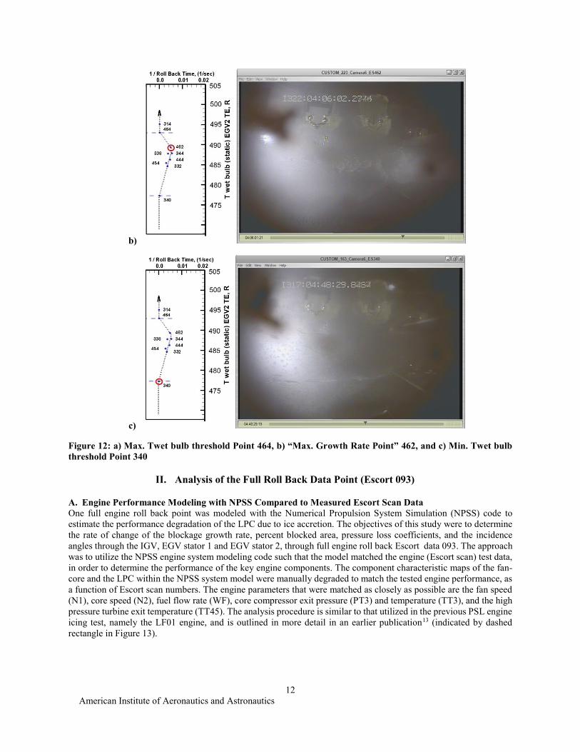
F. Images of Accretion at EGV stator 2 Trailing Edge at Ice-Water Flow to Air Flow Ratio of 0.0021

The images shown in Figure 12 are of three Escort data points at IWAR of 0.0021. Figure 12a) is a no roll back data

point (Escort point 464) that had a calculated wet bulb temperature (493 R) at EGV stator 2 trailing edge. The IWAR

of 0.0021 is near the minimum limit to support accretion, and the small amount of ice that did accrete was slushy with

shedding. The combined effects of relatively low value of IWAR and slightly elevated value of wet bulb temperature

at the stator 2 trailing edge, are suspected to be the reasons the ice did not grow at a significant rate over time, and

consequently did not roll back. Figure 12b) represents the growth of ice for Escort data point 462, which exhibited a

slow called engine roll back (209 seconds). Note that the wet bulb temperature at EGV stator 2 trailing edge was

slightly below freezing (489 R) at this data point. There was slow ice accretion with shedding, but the ice continued

to grow until engine roll back was called by the test engineer. Figure 12c) illustrates the EGV stator 2 trailing edge

for Escort data point 506, showing that there was small amount of ice accretion streaks which did not build up in time,

and no roll back was called. The stator 2 trailing edge wet bulb temperature at this data point was too cold to support

ice accretion, at 477 R.

a)


12

b)

c)

Figure 12: a) Max. Twet bulb threshold Point 464, b) “Max. Growth Rate Point” 462, and c) Min. Twet bulb

threshold Point 340

II. Analysis of the Full Roll Back Data Point (Escort 093)

A. Engine Performance Modeling with NPSS Compared to Measured Escort Scan Data

One full engine roll back point was modeled with the Numerical Propulsion System Simulation (NPSS) code to

estimate the performance degradation of the LPC due to ice accretion. The objectives of this study were to determine

the rate of change of the blockage growth rate, percent blocked area, pressure loss coefficients, and the incidence

angles through the IGV, EGV stator 1 and EGV stator 2, through full engine roll back Escort data 093. The approach

was to utilize the NPSS engine system modeling code such that the model matched the engine (Escort scan) test data,

in order to determine the performance of the key engine components. The component characteristic maps of the fan-

core and the LPC within the NPSS system model were manually degraded to match the tested engine performance, as

a function of Escort scan numbers. The engine parameters that were matched as closely as possible are the fan speed

(N1), core speed (N2), fuel flow rate (WF), core compressor exit pressure (PT3) and temperature (TT3), and the high

pressure turbine exit temperature (TT45). The analysis procedure is similar to that utilized in the previous PSL engine

icing test, namely the LF01 engine, and is outlined in more detail in an earlier publication13 (indicated by dashed

rectangle in Figure 13).


13

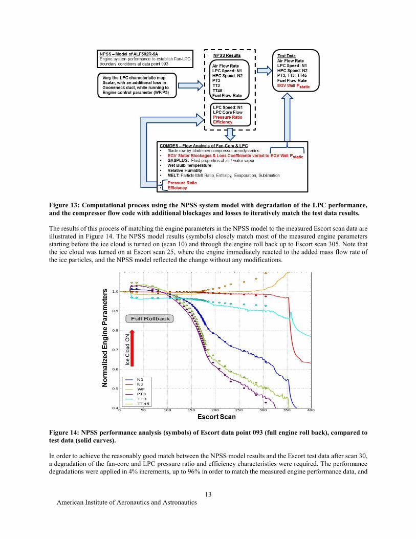
Figure 13: Computational process using the NPSS system model with degradation of the LPC performance,

and the compressor flow code with additional blockages and losses to iteratively match the test data results.

The results of this process of matching the engine parameters in the NPSS model to the measured Escort scan data are

illustrated in Figure 14. The NPSS model results (symbols) closely match most of the measured engine parameters

starting before the ice cloud is turned on (scan 10) and through the engine roll back up to Escort scan 305. Note that

the ice cloud was turned on at Escort scan 25, where the engine immediately reacted to the added mass flow rate of

the ice particles, and the NPSS model reflected the change without any modifications.

Figure 14: NPSS performance analysis (symbols) of Escort data point 093 (full engine roll back), compared to

test data (solid curves).

In order to achieve the reasonably good match between the NPSS model results and the Escort test data after scan 30,

a degradation of the fan-core and LPC pressure ratio and efficiency characteristics were required. The performance

degradations were applied in 4% increments, up to 96% in order to match the measured engine performance data, and


14

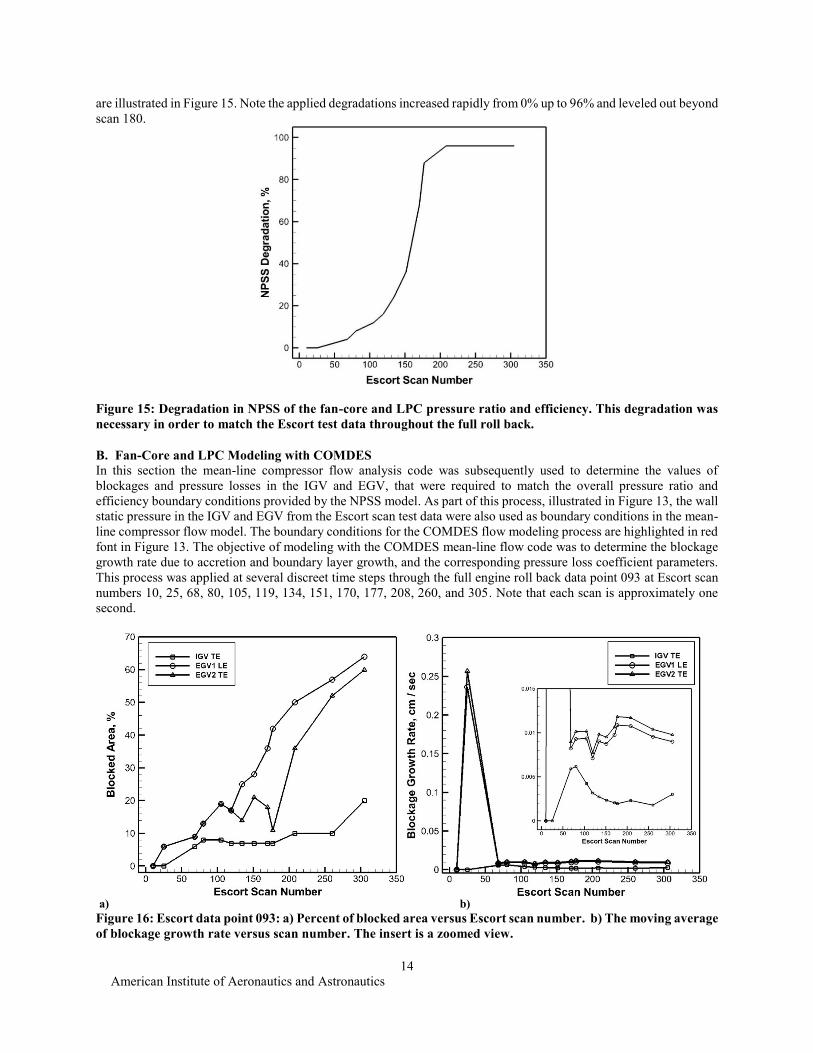
are illustrated in Figure 15. Note the applied degradations increased rapidly from 0% up to 96% and leveled out beyond

scan 180.

Figure 15: Degradation in NPSS of the fan-core and LPC pressure ratio and efficiency. This degradation was

necessary in order to match the Escort test data throughout the full roll back.

B. Fan-Core and LPC Modeling with COMDES

In this section the mean-line compressor flow analysis code was subsequently used to determine the values of

blockages and pressure losses in the IGV and EGV, that were required to match the overall pressure ratio and

efficiency boundary conditions provided by the NPSS model. As part of this process, illustrated in Figure 13, the wall

static pressure in the IGV and EGV from the Escort scan test data were also used as boundary conditions in the mean-

line compressor flow model. The boundary conditions for the COMDES flow modeling process are highlighted in red

font in Figure 13. The objective of modeling with the COMDES mean-line flow code was to determine the blockage

growth rate due to accretion and boundary layer growth, and the corresponding pressure loss coefficient parameters.

This process was applied at several discreet time steps through the full engine roll back data point 093 at Escort scan

numbers 10, 25, 68, 80, 105, 119, 134, 151, 170, 177, 208, 260, and 305. Note that each scan is approximately one

second.

a) b)

Figure 16: Escort data point 093: a) Percent of blocked area versus Escort scan number. b) The moving average

of blockage growth rate versus scan number. The insert is a zoomed view.


15

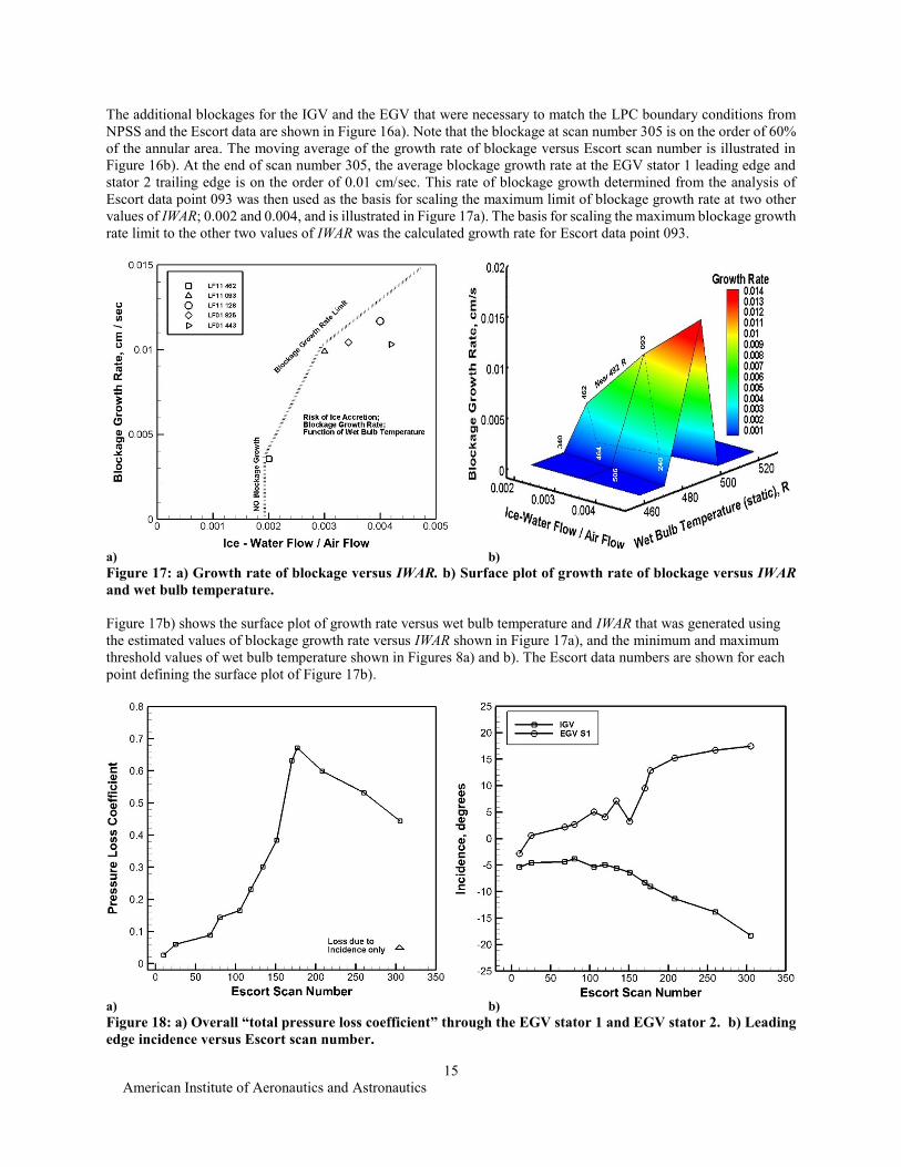
The additional blockages for the IGV and the EGV that were necessary to match the LPC boundary conditions from

NPSS and the Escort data are shown in Figure 16a). Note that the blockage at scan number 305 is on the order of 60%

of the annular area. The moving average of the growth rate of blockage versus Escort scan number is illustrated in

Figure 16b). At the end of scan number 305, the average blockage growth rate at the EGV stator 1 leading edge and

stator 2 trailing edge is on the order of 0.01 cm/sec. This rate of blockage growth determined from the analysis of

Escort data point 093 was then used as the basis for scaling the maximum limit of blockage growth rate at two other

values of IWAR; 0.002 and 0.004, and is illustrated in Figure 17a). The basis for scaling the maximum blockage growth

rate limit to the other two values of IWAR was the calculated growth rate for Escort data point 093.

a) b)

Figure 17: a) Growth rate of blockage versus IWAR. b) Surface plot of growth rate of blockage versus IWAR

and wet bulb temperature.

Figure 17b) shows the surface plot of growth rate versus wet bulb temperature and IWAR that was generated using

the estimated values of blockage growth rate versus IWAR shown in Figure 17a), and the minimum and maximum

threshold values of wet bulb temperature shown in Figures 8a) and b). The Escort data numbers are shown for each

point defining the surface plot of Figure 17b).

a) b)

Figure 18: a) Overall “total pressure loss coefficient” through the EGV stator 1 and EGV stator 2. b) Leading

edge incidence versus Escort scan number.


16

Figure 18a) shows the additional blockage that was required in the compressor flow code to match the NPSS boundary

conditions of the fan-core and LPC total to total pressure ratio and efficiency, as well as the wall static pressure

measurements in the Escort data, as a function of Escort scan number (time). Note that the pressure loss coefficient of

Figure 18a) tracks the performance degradation that was applied to the NPSS model (Figure 15). The total pressure

loss coefficient is primarily due to the time-dependent deterioration of surface roughness caused by the ice accretion.

The losses grew to a value of 0.66 near scan 180, then tapers off to 0.45 at the end of scan 305. This inflection point

is caused by the drastic reduction of the air mass flow rate into the core. However, the local Mach number at the stator

I leading edge and stator 2 trailing edge increases due to the large area reduction that was required to match the

measured wall static pressures, even though the core mass flow rate decreases. The Figure 18b) shows the incidence

versus Escort scan number, as estimated from the compressor flow analysis. Even though the EGV stator 1 incidence

is high at Escort scan 305, the component of pressure loss coefficient due to incidence alone is only 0.05 (See Figure

18a).

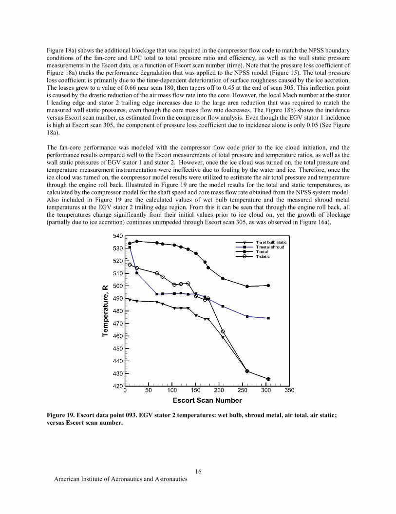
The fan-core performance was modeled with the compressor flow code prior to the ice cloud initiation, and the

performance results compared well to the Escort measurements of total pressure and temperature ratios, as well as the

wall static pressures of EGV stator 1 and stator 2. However, once the ice cloud was turned on, the total pressure and

temperature measurement instrumentation were ineffective due to fouling by the water and ice. Therefore, once the

ice cloud was turned on, the compressor model results were utilized to estimate the air total pressure and temperature

through the engine roll back. Illustrated in Figure 19 are the model results for the total and static temperatures, as

calculated by the compressor model for the shaft speed and core mass flow rate obtained from the NPSS system model.

Also included in Figure 19 are the calculated values of wet bulb temperature and the measured shroud metal

temperatures at the EGV stator 2 trailing edge region. From this it can be seen that through the engine roll back, all

the temperatures change significantly from their initial values prior to ice cloud on, yet the growth of blockage

(partially due to ice accretion) continues unimpeded through Escort scan 305, as was observed in Figure 16a).

Figure 19. Escort data point 093. EGV stator 2 temperatures: wet bulb, shroud metal, air total, air static;

versus Escort scan number.


17

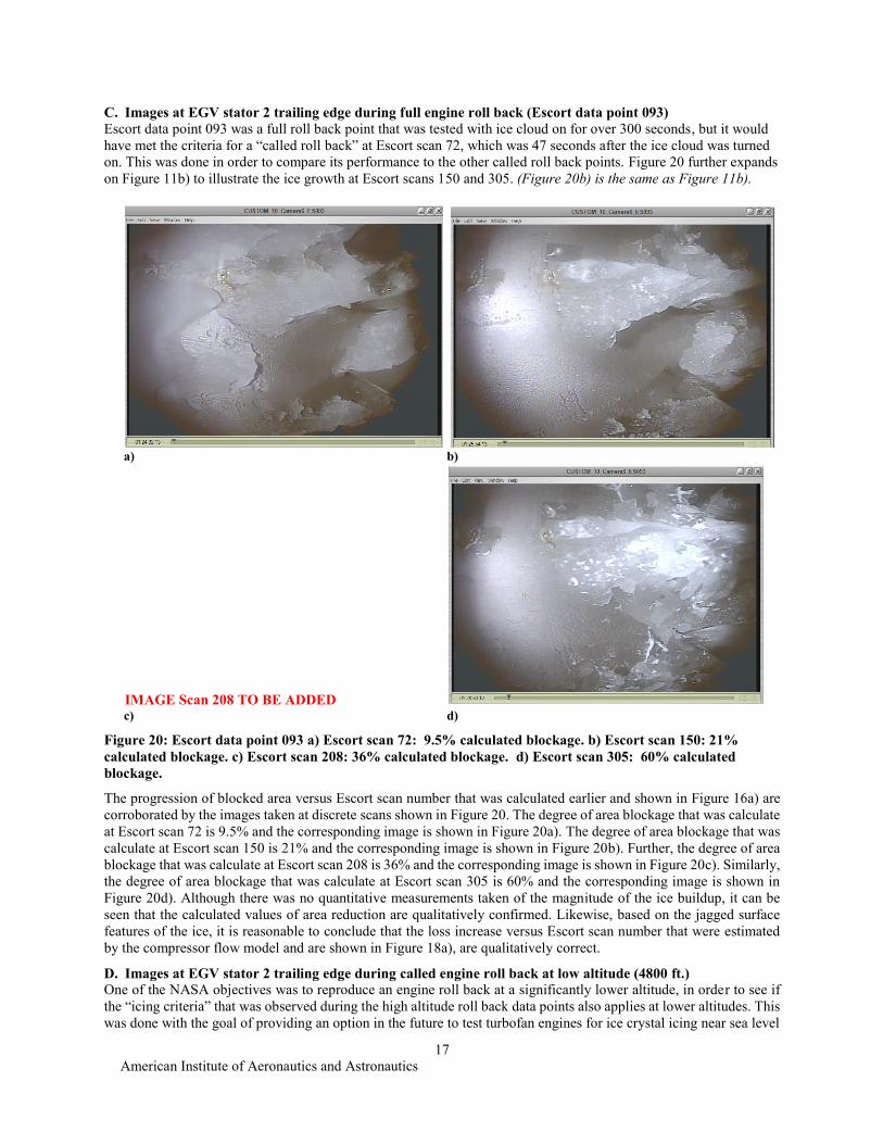
C. Images at EGV stator 2 trailing edge during full engine roll back (Escort data point 093)

Escort data point 093 was a full roll back point that was tested with ice cloud on for over 300 seconds, but it would

have met the criteria for a “called roll back” at Escort scan 72, which was 47 seconds after the ice cloud was turned

on. This was done in order to compare its performance to the other called roll back points. Figure 20 further expands

on Figure 11b) to illustrate the ice growth at Escort scans 150 and 305. (Figure 20b) is the same as Figure 11b).

a) b)

IMAGE Scan 208 TO BE ADDED c) d)

Figure 20: Escort data point 093 a) Escort scan 72: 9.5% calculated blockage. b) Escort scan 150: 21%

calculated blockage. c) Escort scan 208: 36% calculated blockage. d) Escort scan 305: 60% calculated

blockage.

The progression of blocked area versus Escort scan number that was calculated earlier and shown in Figure 16a) are

corroborated by the images taken at discrete scans shown in Figure 20. The degree of area blockage that was calculate

at Escort scan 72 is 9.5% and the corresponding image is shown in Figure 20a). The degree of area blockage that was

calculate at Escort scan 150 is 21% and the corresponding image is shown in Figure 20b). Further, the degree of area

blockage that was calculate at Escort scan 208 is 36% and the corresponding image is shown in Figure 20c). Similarly,

the degree of area blockage that was calculate at Escort scan 305 is 60% and the corresponding image is shown in

Figure 20d). Although there was no quantitative measurements taken of the magnitude of the ice buildup, it can be

seen that the calculated values of area reduction are qualitatively confirmed. Likewise, based on the jagged surface

features of the ice, it is reasonable to conclude that the loss increase versus Escort scan number that were estimated

by the compressor flow model and are shown in Figure 18a), are qualitatively correct.

D. Images at EGV stator 2 trailing edge during called engine roll back at low altitude (4800 ft.)

One of the NASA objectives was to reproduce an engine roll back at a significantly lower altitude, in order to see if

the “icing criteria” that was observed during the high altitude roll back data points also applies at lower altitudes. This

was done with the goal of providing an option in the future to test turbofan engines for ice crystal icing near sea level


18

conditions (without the need for an altitude chamber) at normal ambient temperatures observed in the winter. The PSL

facility lower altitude limit is 4,800 feet. Escort data point 424 achieved a called engine roll back in 138 seconds,

Several data points were taken at this lower altitude (wet bulb temperature plotted in Figure 7). The icing images for

discreet scan numbers from Escort data point 416 are illustrated in Figure 21.

a) b)

c) d)

Figure 21: Escort data point 416; a) Escort scan 86. b) Escort scan 153. c) Escort scan 229. d) Escort scan

429.

The characteristic of the called roll back at low altitude was at reduced levels of wet bulb temperatures, as also seen

in Figure 6. The fastest called roll back was 138 seconds after ice cloud was turned on. This is slower than the fastest

called roll back points that were observed at the higher altitudes near 30,000 feet. Although the images appear to be

cloudy, it is evident that there is ice buildup The images in Figure 21 (Escort data point 416), illustrate one of the

slower roll back points that was called at Escort scan 429. Ice buildup and shedding was observed as illustrated in

Figure 21 b) and c). This ice buildup and shedding process continued through 393 seconds, where the engine roll back

criteria was met.

III. Conclusions

A turbofan engine known to have experienced an icing event at high altitudes and operating conditions during flight

through convective ice crystal clouds was tested in the NASA Propulsion Systems Laboratory (PSL) simulated altitude

engine test facility. The NPSS system model with parameter degradation of the LPC closely matched the measured

engine performance of the full engine roll back data point.

The rate of blockage growth due to ice accretion is a function of the local wet bulb temperature as well as the ratio of

ice-water-flow-rate to air-flow-rate (IWAR). The minimum value IWAR for engine roll back is on the order of 0.002.


19

For a given IWAR, the highest rate of (ice) blockage growth rate is a function of the wet bulb temperature at the EGV

stator 2 trailing edge.

Based on this study, the upper limit of wet bulb temperature at stator 2 trailing edge is in the range of 493 - 497 R for

ice accretion to occur. Likewise, the lower limit of wet bulb temperature at stator 2 trailing edge is in the range of 475

- 477 R in order for ice accretion to occur.

The video images of the EGV stator 2 trailing edge verify qualitatively that the area blockage which was estimated by

compressor flow analysis can be attributed to ice accretion. However boundary layer growth is also a factor in the area

blockage, but it has not been quantified.

Based on the data analysis results, a model was created, and consists of a general relation of the blockage growth

versus the wet bulb temperature and the ratio of ice-water-flow-rate to-air-flow-rate (IWAR). The corresponding rate

of pressure loss coefficient is related to the percent of blocked annular area.

During the full roll back point (Escort 093) there is a large increase in pressure loss coefficient in the tandem stator

EGV, and is estimated to be mainly due to deteriorated surface roughness, and only minimally due to leading edge

incidence loss effects. The temperatures at the EGV stator 2 region change significantly from their initial values prior

to the ice cloud being turned on, yet the growth of blockage (partially due to ice accretion) continues unimpeded at

the same rate through the engine roll back.

A low altitude engine called roll back was achieved at 4,800 feet in a similar time scale as those observed at high

altitude (near 30,000 feet) at comparable values of IWAR. However, the wet bulb temperature to achieve accretion

was lower than at the higher altitudes.

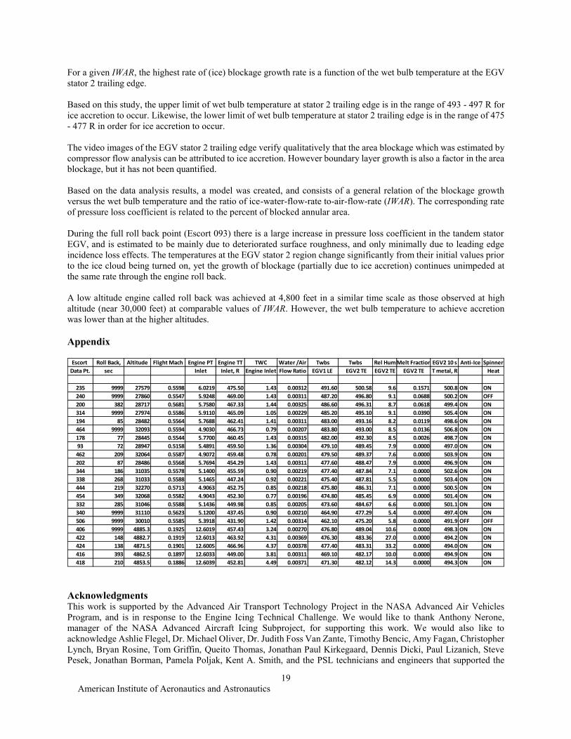
Appendix

Acknowledgments This work is supported by the Advanced Air Transport Technology Project in the NASA Advanced Air Vehicles

Program, and is in response to the Engine Icing Technical Challenge. We would like to thank Anthony Nerone,

manager of the NASA Advanced Aircraft Icing Subproject, for supporting this work. We would also like to

acknowledge Ashlie Flegel, Dr. Michael Oliver, Dr. Judith Foss Van Zante, Timothy Bencic, Amy Fagan, Christopher

Lynch, Bryan Rosine, Tom Griffin, Queito Thomas, Jonathan Paul Kirkegaard, Dennis Dicki, Paul Lizanich, Steve

Pesek, Jonathan Borman, Pamela Poljak, Kent A. Smith, and the PSL technicians and engineers that supported the

Escort Roll Back, Altitude Flight Mach Engine PT Engine TT TWC Water /Air Twbs Twbs Rel Hum Melt Fraction EGV2 10 s Anti-Ice Spinner

Data Pt. sec Inlet Inlet, R Engine Inlet Flow Ratio EGV1 LE EGV2 TE EGV2 TE EGV2 TE T metal, R Heat

235 9999 27579 0.5598 6.0219 475.50 1.43 0.00312 491.60 500.58 9.6 0.1571 500.8 ON ON

240 9999 27860 0.5547 5.9248 469.00 1.43 0.00311 487.20 496.80 9.1 0.0688 500.2 ON OFF

200 382 28717 0.5681 5.7580 467.33 1.44 0.00325 486.60 496.31 8.7 0.0618 499.4 ON ON

314 9999 27974 0.5586 5.9110 465.09 1.05 0.00229 485.20 495.10 9.1 0.0390 505.4 ON ON

194 85 28482 0.5564 5.7688 462.41 1.41 0.00311 483.00 493.16 8.2 0.0119 498.6 ON ON

464 9999 32093 0.5594 4.9030 466.73 0.79 0.00207 483.80 493.00 8.5 0.0136 506.8 ON ON

178 77 28445 0.5544 5.7700 460.45 1.43 0.00315 482.00 492.30 8.5 0.0026 498.7 ON ON

93 72 28947 0.5158 5.4891 459.50 1.36 0.00304 479.10 489.45 7.9 0.0000 497.0 ON ON

462 209 32064 0.5587 4.9072 459.48 0.78 0.00201 479.50 489.37 7.6 0.0000 503.9 ON ON

202 87 28486 0.5568 5.7694 454.29 1.43 0.00311 477.60 488.47 7.9 0.0000 496.9 ON ON

344 186 31035 0.5578 5.1400 455.59 0.90 0.00219 477.40 487.84 7.1 0.0000 502.6 ON ON

338 268 31033 0.5588 5.1465 447.24 0.92 0.00221 475.40 487.81 5.5 0.0000 503.4 ON ON

444 219 32270 0.5713 4.9063 452.75 0.85 0.00218 475.80 486.31 7.1 0.0000 500.5 ON ON

454 349 32068 0.5582 4.9043 452.30 0.77 0.00196 474.80 485.45 6.9 0.0000 501.4 ON ON

332 285 31046 0.5588 5.1436 449.98 0.85 0.00205 473.60 484.67 6.6 0.0000 501.1 ON ON

340 9999 31110 0.5623 5.1200 437.45 0.90 0.00210 464.90 477.29 5.4 0.0000 497.4 ON ON

506 9999 30010 0.5585 5.3918 431.90 1.42 0.00314 462.10 475.20 5.8 0.0000 491.9 OFF OFF

406 9999 4885.3 0.1925 12.6019 457.43 3.24 0.00270 476.80 489.04 10.6 0.0000 498.3 ON ON

422 148 4882.7 0.1919 12.6013 463.92 4.31 0.00369 476.30 483.36 27.0 0.0000 494.2 ON ON

424 138 4871.5 0.1901 12.6005 466.96 4.37 0.00378 477.40 483.31 33.2 0.0000 494.0 ON ON

416 393 4862.5 0.1897 12.6033 449.00 3.81 0.00311 469.10 482.17 10.0 0.0000 494.9 ON ON

418 210 4853.5 0.1886 12.6039 452.81 4.49 0.00371 471.30 482.12 14.3 0.0000 494.3 ON ON


20

test and facility development at NASA Glenn Research Center for providing the excellent test data for this engine in

the unique altitude test facility with spray bars that successfully simulated ice ingestion testing. We also acknowledge

the help and guidance we received from Dr. William B. Wright (Vantage Partners, LLC.) for guidance in providing

the MELT code and Dr. Jen-Ching Tsao (Ohio Aerospace Institute) for his insights and analyses.

References 1Mason, J. G., Chow, P., Fuleki, D. M., “Understanding Ice Crystal Accretion and Shedding Phenomenon in Jet Engines Using a

Rig Test,” GT2010-22550. 2Mason, J. G., Grzych, M., “The Challenges Identifying Weather Associated With Jet Engine Ice Crystal Icing,” SAE 2011-38-

0094. 3Goodwin, R. V., Dischinger, D. G., “Turbofan Ice Crystal Rollback Investigation and Preparations Leading to Inaugural Ice

Crystal Engine Test at NASA PSL-3 Test Facility,” AIAA 2014-2895. 4Oliver, M. J., “Validation Ice Crystal Icing Engine Test in the Propulsion Systems Laboratory at NASA Glenn Research Center,”

AIAA-2014-2898. 5Van Zante, Judith F. (and?), “Update on the NASA Glenn Propulsion Systems Lab Ice Crystal Cloud Characterization

(2015)”, submitted to 2016 AIAA Aviation. 8th AIAA Atmospheric and Space Environments Conference, 2016 AIAA

Aviation.

6Jorgenson, P. C. E., Veres, J. P., Jones, S. M., “Modeling the Deterioration of Engine and Low Pressure Compressor Performance

During a Roll Back Event due to Ice Accretion,” AIAA-2014-3842. 7Veres, J. P., Jones, S. M., Jorgenson, P. C. E., “Performance Modeling of Honeywell Turbofan Engine Tested with Ice Crystal

Ingestion in the NASA Propulsion System Laboratory,” SAE-2015-01-2133. 8Veres, J. P., “Axial and Centrifugal Compressor Mean Line Flow Analysis Method,” AIAA-2009-1641, NASA/TM-2009-215585. 9Veres, J. P., Jorgenson, P. C. E., Wright, W. B., Struk, P., “A Model to Assess the Risk of Ice Accretion due to Ice Crystal Ingestion

in a Turbofan Engine and its Effects on Performance,” AIAA 2012-3038. 10Veres, J. P., Jorgenson, P. C. E., “Modeling Commercial Turbofan Engine Icing Risk with Ice Crystal Ingestion,” AIAA 2013-

2679. 11Veres, J. P., Jorgenson, P. C. E., Coennen R., “Modeling Commercial Turbofan Engine Icing Risk with Ice Crystal Ingestion;

Follow-On,” AIAA 2014-2899. 12Struk, P., Currie, T., Wright, W. B., Tsao, J.-C., Broeren, A., Vargas, M., Knezevici, D., and Fuleki, D., “Fundamental Ice Crystal

Accretion Physics Studies,” SAE-11ICE-0034, 2011. 13Currie, T. C., Struk, P. M., Tsao, J.-C., Fuleki, D., Knezevici, D., “Fundamental Study of Mixed-Phase Icing with Application to

Ice Crystal Accretion in Aircraft Jet Engines,” AIAA-2012-3035.

Documents

Modeling of Highly Instrumented Honeywell Turbofan Engine ...Modeling of Highly Instrumented Honeywell Turbofan Engine Tested with Ice Crystal Ingestion in the NASA Propulsion System