Embed Size (px)
Citation preview
Modeling of High-TemperatureCreep for Structural Analysis
Applications
Habilitationsschrift
zur Erlangung des akademischen Grades
Dr.-Ing. habil.
vorgelegt der
Mathematisch-Naturwissenschaftlich-Technischen Fakultatder Martin-Luther-Universitat Halle-Wittenberg
von
Herrn Dr.-Ing. Konstantin Naumenko
geb. am 3.08.1966 in Kharkov (Ukraine)
Gutachter:
1. Prof. Holm Altenbach, Halle (Saale)
2. Prof. Reinhold Kienzler, Bremen
3. Prof. Jacek Skrzypek, Krakow
Halle (Saale), 12. April 2006
urn:nbn:de:gbv:3-000010187[http://nbn-resolving.de/urn/resolver.pl?urn=nbn%3Ade%3Agbv%3A3-000010187]


Vorwort
Die vorliegende Arbeit entstand wahrend meiner Tatigkeit als wissenschaftlicherMitarbeiter am Institut fur Prozess- und Stoffmodellierung der Martin-Luther-Universitat Halle-Wittenberg.
Von Herrn Professor H. Altenbach wurde ich zu dieser Arbeit angeregt. Ich mochteihm ganz herzlich fur die Motivation, großzugige Unterstutzung sowie fur die Be-gutachtung dieser Arbeit danken.
Mein herzlicher Dank gilt Herrn Professor R. Kienzler und Herrn ProfessorJ. Skrzypek fur die freundlicheUbernahme der Begutachtung, fur das Interesse andieser Arbeit und wertvolle Hinweise.
Weiterhin danke ich Herrn Professor J. Altenbach, Herrn Professor O. K. Mo-rachkowsky und Herrn Professor P. A. Zhilin fur zahlreicheAnregungen, die zurEntstehung und der Abrundung dieser Arbeit beigetragen haben.
Nicht zuletzt danke ich allen Mitarbeitern des Lehrstuhls fur Technische Mechanikfur ihre Hilfe, konstruktive Diskussionen sowie das angenehme Arbeitsklima.
Mein besonderer Dank gilt meiner Familie, ohne deren liebevolle Unterstutzungdiese Arbeit nicht moglich gewesen ware.
Halle (Saale), im April 2006
Konstantin Naumenko
Abstract
For many structures designed for high temperature applications, e.g. piping systemsand pressure vessels, an important problem is the life time assessment in the creeprange. The objective of this work is to present an extensive overview about the the-oretical modeling and numerical analysis of creep and long-term strength of struc-tures. The study deals with three principal topics including constitutive equationsfor creep in structural materials under multi-axial stressstates, structural mechanicsmodels of beams, plates, shells and three-dimensional solids, and numerical proce-dures for the solution of initial-boundary value problems of creep mechanics.
Within the framework of the constitutive modeling we discuss various exten-sions of the von Mises-Odqvist type creep theory to take intoaccount stress stateeffects, anisotropy as well as hardening and damage processes. For several casesof material symmetries appropriate invariants of the stress tensor, equivalent stressand strain expressions as well as creep constitutive equations are derived. Primarycreep and transient creep effects can be described by the introduction of harden-ing state variables. Models of time, strain and kinematic hardening are examinedas they characterize multi-axial creep behavior under simple and non-proportionalloading conditions. A systematic review and evaluation of constitutive equationswith damage variables and corresponding evolution equations recently applied todescribe tertiary creep and long term strength is presented. Stress state effects oftertiary creep and the damage induced anisotropy are discussed in detail.
For several structural materials creep curves, constitutive equations, responsefunctions and material constants are summarized accordingto recently publisheddata. Furthermore, a new model describing anisotropic creep in a multi-pass weldmetal is presented.
Governing equations for creep in three-dimensional solidsare introduced to for-mulate initial-boundary value problems, variational procedures and time step algo-rithms. Various structural mechanics models of beams, plates and shells are dis-cussed in context of their applicability to creep problems.Emphasis is placed oneffects of transverse shear deformations, boundary layersand geometrical nonlin-earities.
A model with a scalar damage variable is incorporated into the ANSYS finiteelement code by means of a user defined material subroutine. To verify the sub-routine several benchmark problems are developed and solved by special numericalmethods. Results of finite element analysis for the same problems illustrate the ap-plicability of the developed subroutine over a wide range ofelement types includingshell and solid elements. Furthermore, they show the influence of the mesh size onthe accuracy of solutions. Finally an example for long term strength analysis of aspatial steam pipeline is presented. The results show that the developed approach iscapable to reproduce basic features of creep and damage processes in engineeringstructures.
Zusammenfassung
Fur zahlreiche Bauteile fur Hochtemperaturanwendungenist die Lebensdauerab-schatzung im Kriechbereich die wichtigste Aufgabe bei derVorbereitung von Ein-satzentscheidungen. Ziel dieser Arbeit ist es, einen umfassendenUberblick uber dietheoretische Modellierung und die Analyse des Kriechens und der Langzeitfestig-keit von Bauteilen zu geben. Dabei stehen folgende Schwerpunkte im Mittelpunkt:Konstitutivgleichungen fur das Kriechen von Ingenieurwerkstoffen unter mehrach-sigen Beanspruchungen, strukturmechanische Modelle furBalken, Platten, Schalenund dreidimensionale Korper sowie numerische Verfahren fur die Losung nichtli-nearer Anfangs-Randwertaufgaben der Kriechmechanik.
Im Rahmen der konstitutiven Modellierung werden zahlreiche Erweiterungender Mises-Odqvist-Kriechtheorie wie die Einbeziehung derArt des Spannungszu-standes, der Anisotropie sowie der Verfestigungs- und Sch¨adigungsvorgange dis-kutiert. Fur Sonderfalle der Materialsymmetrien werdengeeignete Invarianten desSpannungstensors, Ansatze fur Vergleichsspannungen und -dehnungen sowie Kon-stitutivgleichungen zum anisotropen Kriechen formuliert. Das Primarkriechen undtransiente Kriechvorgange konnen durch die Einfuhrungvon Verfestigungsvaria-blen beschrieben werden. Die Modelle der Zeit- und Deformations- sowie der kine-matischen Verfestigung werden bezuglich der Vorhersagbarkeit des mehrachsigenKriechens untersucht. Danach erfolgen ein systematischerUberblick und die Be-wertung der Konstitutivgleichungen mit Schadigungsvariablen, die bisher auf dieBeschreibung des Tertiarkriechens und der Langzeitfestigkeit angewandt wurden.
Fur einige Ingenieurwerkstoffe werden Kriechkurven, Konstitutivgleichungen,konstitutive Funktionen und Werkstoffkennwerte anhand der in der Literatur publi-zierten Daten zusammengefasst. Ferner wird ein neues Modell zur Beschreibungdes anisotropen Kriechens in einem mehrlagigen Schweißgutvorgestellt.
Die Grundgleichungen fur das Kriechen in dreidimensionalen Korpern werdenzum Zweck der Formulierung von Anfangs-Randwertproblemen, Variationsverfah-ren und Zeitschrittalgorithmen zusammengefasst. Zahlreiche Modelle der Struktur-mechanik fur Balken, Platten und Schalen werden bezuglich ihrer Anwendbarkeitauf Kriechprobleme diskutiert. Hier wird auf Effekte wie Querschubverzerrung,Randschichten und geometrische Nichtlineatitaten aufmerksam gemacht.
Modelle mit Schadigungsvariablen werden mit Hilfe einer benutzerdefiniertensubroutine in das Programmsystem ANSYS eingebunden. Fur deren Verifikationwerden Testaufgaben entwickelt und mit Hilfe spezieller numerischer Verfahrengelost. Berechnungen der selben Aufgaben mit der Methode der finiten Elementeillustrieren die Anwendbarkeit der entwickelten subroutine fur verschiedene Ty-pen von finiten Elementen. Weiterhin zeigen sie den Einfluss der Netzdichte aufdie Losungsgenauigkeit. Abschließend wird die Langzeitfestigkeitsanalyse einerraumlichen Rohrleitung vorgestellt. Die Ergebnisse zeigen, dass das entwickelteVerfahren in der Lage ist, die wesentlichen Kriech- und Sch¨adigungsvorgange inIngenieurkonstruktionen darzustellen.

VI
Contents
1 Introduction . . . . . . . . . . . . . . . . . . . . . . . . . . . . . . . . . . . . . . . . . . . . . . . . . . 11.1 Creep Phenomena in Structural Materials . . . . . . . . . . . . .. . . . . . . . . 1
1.1.1 Uni-Axial Creep . . . . . . . . . . . . . . . . . . . . . . . . . . . . . . . .. . . . . 11.1.2 Multi-Axial Creep and Stress State Effects . . . . . . . . .. . . . . . 7
1.2 Creep in Engineering Structures . . . . . . . . . . . . . . . . . . . .. . . . . . . . . . 111.3 State of the Art in Creep Modeling . . . . . . . . . . . . . . . . . . . .. . . . . . . . 151.4 Scope and Outline . . . . . . . . . . . . . . . . . . . . . . . . . . . . . . . . .. . . . . . . . . 17
2 Constitutive Models of Creep . . . . . . . . . . . . . . . . . . . . . . . . . . . . . . . . . 192.1 General Remarks . . . . . . . . . . . . . . . . . . . . . . . . . . . . . . . . . .. . . . . . . . . 192.2 Secondary Creep . . . . . . . . . . . . . . . . . . . . . . . . . . . . . . . . . .. . . . . . . . . 25
2.2.1 Isotropic Creep . . . . . . . . . . . . . . . . . . . . . . . . . . . . . . . .. . . . . . 252.2.1.1 Classical Creep Equations . . . . . . . . . . . . . . . . . . . . .252.2.1.2 Creep Potentials with Three Invariants of the
Stress Tensor . . . . . . . . . . . . . . . . . . . . . . . . . . . . . . . . 272.2.2 Creep of Initially Anisotropic Materials . . . . . . . . . .. . . . . . . 31
2.2.2.1 Classical Creep Equations . . . . . . . . . . . . . . . . . . . . .322.2.2.2 Non-classical Creep Equations . . . . . . . . . . . . . . . . .40
2.2.3 Functions of Stress and Temperature . . . . . . . . . . . . . . .. . . . . 462.3 Primary Creep and Creep Transients . . . . . . . . . . . . . . . . . .. . . . . . . . . 51
2.3.1 Time and Strain Hardening . . . . . . . . . . . . . . . . . . . . . . . .. . . . 542.3.2 Kinematic Hardening . . . . . . . . . . . . . . . . . . . . . . . . . . . .. . . . . 56
2.4 Tertiary Creep and Creep Damage . . . . . . . . . . . . . . . . . . . . .. . . . . . . 632.4.1 Scalar-Valued Damage Variables . . . . . . . . . . . . . . . . . .. . . . . 64
2.4.1.1 Kachanov-Rabotnov Model . . . . . . . . . . . . . . . . . . . 642.4.1.2 Micromechanically-Consistent Models . . . . . . . . . .732.4.1.3 Mechanism-Based Models . . . . . . . . . . . . . . . . . . . . 752.4.1.4 Models Based on Dissipation . . . . . . . . . . . . . . . . . . 77
2.4.2 Damage-Induced Anisotropy . . . . . . . . . . . . . . . . . . . . . .. . . . 78
3 Examples of Constitutive Equations for Selected Material s . . . . 853.1 Models of Isotropic Creep for Several Alloys . . . . . . . . . .. . . . . . . . . 86
3.1.1 Type 316 Steel . . . . . . . . . . . . . . . . . . . . . . . . . . . . . . . . . .. . . . 863.1.2 Steel 13CrMo4-5 . . . . . . . . . . . . . . . . . . . . . . . . . . . . . . . .. . . . 87
VIII Contents
3.1.3 Aluminium Alloy D16AT . . . . . . . . . . . . . . . . . . . . . . . . . . .. . 873.1.4 Aluminium Alloy BS 1472 . . . . . . . . . . . . . . . . . . . . . . . . . .. . 87
3.2 Model for Anisotropic Creep in a Multi-Pass Weld Metal . .. . . . . . . 913.2.1 Origins of Anisotropic Creep . . . . . . . . . . . . . . . . . . . . .. . . . . 933.2.2 Modeling of Secondary Creep . . . . . . . . . . . . . . . . . . . . . .. . . 983.2.3 Identification of Material Constants . . . . . . . . . . . . . .. . . . . . . 99
4 Modeling of Creep in Structures . . . . . . . . . . . . . . . . . . . . . . . . . . . . . . 1034.1 General Remarks . . . . . . . . . . . . . . . . . . . . . . . . . . . . . . . . . .. . . . . . . . . 1034.2 Initial-Boundary Value Problems and General Solution Procedures . 106
4.2.1 Governing Equations . . . . . . . . . . . . . . . . . . . . . . . . . . . .. . . . . 1064.2.2 Vector-Matrix Representation . . . . . . . . . . . . . . . . . . .. . . . . . . 1084.2.3 Numerical Solution Techniques . . . . . . . . . . . . . . . . . . .. . . . . 111
4.2.3.1 Time Integration Methods . . . . . . . . . . . . . . . . . . . . . 1124.2.3.2 Solution of Boundary Value Problems . . . . . . . . . . . 1174.2.3.3 Variational Formulations and Procedures . . . . . . . .118
4.3 Beams . . . . . . . . . . . . . . . . . . . . . . . . . . . . . . . . . . . . . . . . . . .. . . . . . . . . 1234.3.1 Classical Beam Theory . . . . . . . . . . . . . . . . . . . . . . . . . . .. . . . 123
4.3.1.1 Governing Equations . . . . . . . . . . . . . . . . . . . . . . . . . 1234.3.1.2 Closed Form Solutions . . . . . . . . . . . . . . . . . . . . . . . 1254.3.1.3 Approximate Solutions by the Ritz Method . . . . . . 1264.3.1.4 Example . . . . . . . . . . . . . . . . . . . . . . . . . . . . . . . . . . . 128
4.3.2 Refined Theories of Beams . . . . . . . . . . . . . . . . . . . . . . . . .. . . 1324.3.2.1 Stress State Effects and Cross Section Assumptions1324.3.2.2 First Order Shear Deformation Equations . . . . . . . . 1344.3.2.3 Example . . . . . . . . . . . . . . . . . . . . . . . . . . . . . . . . . . . 138
4.4 Plates and Shells . . . . . . . . . . . . . . . . . . . . . . . . . . . . . . . . .. . . . . . . . . . 1424.4.1 Approaches to the Analysis of Plates and Shells . . . . . .. . . . . 1424.4.2 Examples . . . . . . . . . . . . . . . . . . . . . . . . . . . . . . . . . . . . . .. . . . . 145
4.4.2.1 Edge Effects in a Moderately-Thick Plate . . . . . . . . 1454.4.2.2 Long Term Strength Analysis of a Steam Transfer
Line . . . . . . . . . . . . . . . . . . . . . . . . . . . . . . . . . . . . . . . 154
5 Conclusions . . . . . . . . . . . . . . . . . . . . . . . . . . . . . . . . . . . . . . . . . . . . . . . . . . 163
A Some Basic Rules of Tensor Calculus . . . . . . . . . . . . . . . . . . . . . . . . 167A.1 Basic Operations of Tensor Algebra . . . . . . . . . . . . . . . . . .. . . . . . . . . 168
A.1.1 Polar and Axial Vectors . . . . . . . . . . . . . . . . . . . . . . . . . .. . . . . 168A.1.2 Operations with Vectors . . . . . . . . . . . . . . . . . . . . . . . . .. . . . . . 169A.1.3 Bases . . . . . . . . . . . . . . . . . . . . . . . . . . . . . . . . . . . . . . . . .. . . . . 171A.1.4 Operations with Second Rank Tensors . . . . . . . . . . . . . . .. . . . 172
A.2 Elements of Tensor Analysis . . . . . . . . . . . . . . . . . . . . . . . .. . . . . . . . . 178A.2.1 Coordinate Systems . . . . . . . . . . . . . . . . . . . . . . . . . . . . .. . . . . 178A.2.2 The Hamilton (Nabla) Operator . . . . . . . . . . . . . . . . . . . .. . . . 180A.2.3 Integral Theorems . . . . . . . . . . . . . . . . . . . . . . . . . . . . . .. . . . . 181

Contents IX
A.2.4 Scalar-Valued Functions of Vectors and Second Rank Tensors182A.3 Orthogonal Transformations and Orthogonal Invariants. . . . . . . . . . . 182
A.3.1 Invariants for the Full Orthogonal Group . . . . . . . . . . .. . . . . . 184A.3.2 Invariants for the Transverse Isotropy Group . . . . . . .. . . . . . 184A.3.3 Invariants for the Orthotropic Symmetry Group . . . . . .. . . . . 191

X Contents
1 Introduction
Creep is the progressive time-dependent inelastic deformation under constant loadand temperature. Relaxation is the time-dependent decrease of stress under the con-dition of constant deformation and temperature. For many structural materials, forexample steel, both the creep and the relaxation can be observed above a certaincritical temperature. The creep process is accompanied by many different slow mi-crostructural rearrangements including dislocation movement, ageing of microstruc-ture and grain-boundary cavitation.
The above definitions of creep and relaxation are related to the case of uni-axialhomogeneous stress states realized in standard material testing. Under “creep instructures” we understand time-dependent changes of strain and stress states takingplace in structural components as a consequence of externalloading and tempera-ture. Examples of these changes include progressive deformations, relaxation andredistribution of stresses, local reduction of material strength, etc. Furthermore, thestrain and stress states are inhomogeneous and multi-axialin most cases. The scopeof “creep modeling for structural analysis” is to develop a tool which allows to sim-ulate the time-dependent behavior in engineering structures up to the critical stateof creep rupture.
In Chapter 1 we discuss basic features of creep behavior of materials and struc-tures, present the state of the art within the framework of creep modeling and definethe scope of this contribution.
1.1 Creep Phenomena in Structural Materials
The analysis of the material behavior can be based on different experimental ob-servations, for example, macroscopic and microscopic. Theengineering approachis related to the stress-strain analysis of structures and mostly based on the standardmechanical tests. In this section we discuss basic featuresof the creep behavior ac-cording to recently published results of creep testing under uni-axial and multi-axialstress states.
1.1.1 Uni-Axial Creep
Uni-axial creep tests belong to the basic experiments of thematerial behavior eval-uation. A standard cylindrical tension specimen is heated up to the temperature
2 1 Introduction
time (t)
stra
in(ε)
nnn
F
F
F = const, T = const,σσσ = σnnn ⊗ nnn, σ = F/A0
σ < σy, 0.3Tm < T < 0.5Tm
T
minimum creep rateIII
III
fracture
instantaneous elastic strainεel
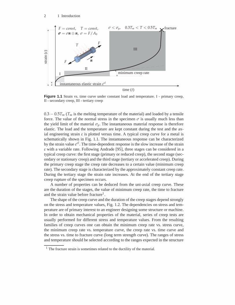
Figure 1.1 Strain vs. time curve under constant load and temperature. I- primary creep,II - secondary creep, III - tertiary creep
0.3 − 0.5Tm (Tm is the melting temperature of the material) and loaded by a tensileforce. The value of the normal stress in the specimenσ is usually much less thanthe yield limit of the materialσy. The instantaneous material response is thereforeelastic. The load and the temperature are kept constant during the test and the ax-ial engineering strainε is plotted versus time. A typical creep curve for a metal isschematically shown in Fig. 1.1. The instantaneous response can be characterizedby the strain valueεel . The time-dependent response is the slow increase of the strainε with a variable rate. Following Andrade [95], three stages can be considered in atypical creep curve: the first stage (primary or reduced creep), the second stage (sec-ondary or stationary creep) and the third stage (tertiary oraccelerated creep). Duringthe primary creep stage the creep rate decreases to a certainvalue (minimum creeprate). The secondary stage is characterized by the approximately constant creep rate.During the tertiary stage the strain rate increases. At the end of the tertiary stagecreep rupture of the specimen occurs.
A number of properties can be deduced from the uni-axial creep curve. Theseare the duration of the stages, the value of minimum creep rate, the time to fractureand the strain value before fracture1.
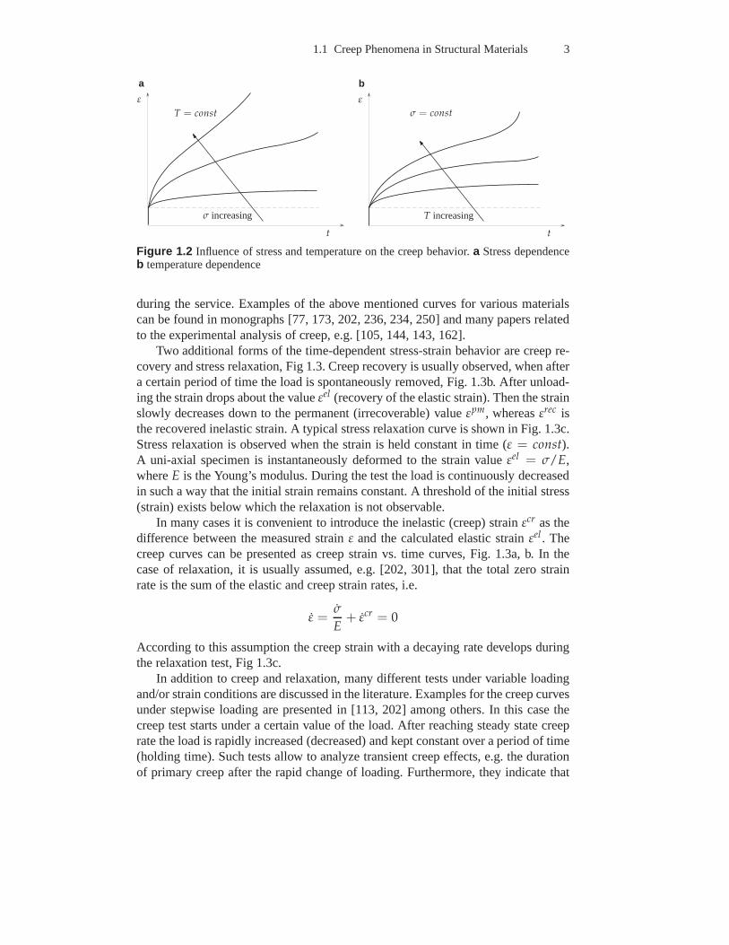
The shape of the creep curve and the duration of the creep stages depend stronglyon the stress and temperature values, Fig. 1.2. The dependencies on stress and tem-perature are of primary interest to an engineer designing some structure or machine.In order to obtain mechanical properties of the material, series of creep tests areusually performed for different stress and temperature values. From the resultingfamilies of creep curves one can obtain the minimum creep rate vs. stress curve,the minimum creep rate vs. temperature curve, the creep ratevs. time curve andthe stress vs. time to fracture curve (long term strength curve). The ranges of stressand temperature should be selected according to the ranges expected in the structure
1 The fracture strain is sometimes related to the ductility ofthe material.
1.1 Creep Phenomena in Structural Materials 3
replacements
t t
ε ε
σ = const
T increasing
T = const
σ increasing
a b
Figure 1.2 Influence of stress and temperature on the creep behavior.a Stress dependenceb temperature dependence
during the service. Examples of the above mentioned curves for various materialscan be found in monographs [77, 173, 202, 236, 234, 250] and many papers relatedto the experimental analysis of creep, e.g. [105, 144, 143, 162].
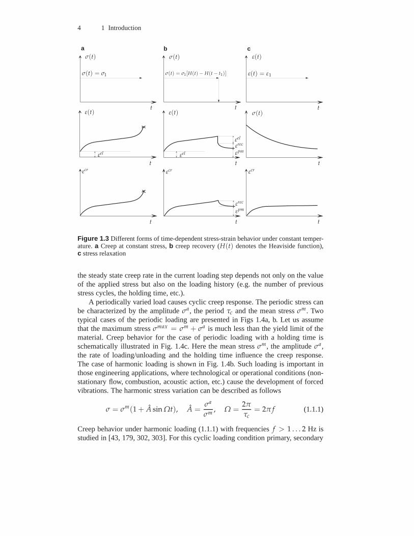
Two additional forms of the time-dependent stress-strain behavior are creep re-covery and stress relaxation, Fig 1.3. Creep recovery is usually observed, when aftera certain period of time the load is spontaneously removed, Fig. 1.3b. After unload-ing the strain drops about the valueεel (recovery of the elastic strain). Then the strainslowly decreases down to the permanent (irrecoverable) value εpm, whereasεrec isthe recovered inelastic strain. A typical stress relaxation curve is shown in Fig. 1.3c.Stress relaxation is observed when the strain is held constant in time (ε = const).A uni-axial specimen is instantaneously deformed to the strain valueεel = σ/E,whereE is the Young’s modulus. During the test the load is continuously decreasedin such a way that the initial strain remains constant. A threshold of the initial stress(strain) exists below which the relaxation is not observable.
In many cases it is convenient to introduce the inelastic (creep) strainεcr as thedifference between the measured strainε and the calculated elastic strainεel . Thecreep curves can be presented as creep strain vs. time curves, Fig. 1.3a, b. In thecase of relaxation, it is usually assumed, e.g. [202, 301], that the total zero strainrate is the sum of the elastic and creep strain rates, i.e.
ε =σ
E+ εcr = 0
According to this assumption the creep strain with a decaying rate develops duringthe relaxation test, Fig 1.3c.
In addition to creep and relaxation, many different tests under variable loadingand/or strain conditions are discussed in the literature. Examples for the creep curvesunder stepwise loading are presented in [113, 202] among others. In this case thecreep test starts under a certain value of the load. After reaching steady state creeprate the load is rapidly increased (decreased) and kept constant over a period of time(holding time). Such tests allow to analyze transient creepeffects, e.g. the durationof primary creep after the rapid change of loading. Furthermore, they indicate that
4 1 Introduction
ttt
ttt
tttσ(t)
σ(t)σ(t)
ε(t)ε(t)
ε(t)
σ(t) = σ1 σ(t) = σ1[H(t) − H(t − t1)] ε(t) = ε1
εel
εelεel
εrec
εrec
εpm
εpm
εcrεcrεcr
a b c
Figure 1.3 Different forms of time-dependent stress-strain behaviorunder constant temper-ature.a Creep at constant stress,b creep recovery (H(t) denotes the Heaviside function),c stress relaxation
the steady state creep rate in the current loading step depends not only on the valueof the applied stress but also on the loading history (e.g. the number of previousstress cycles, the holding time, etc.).
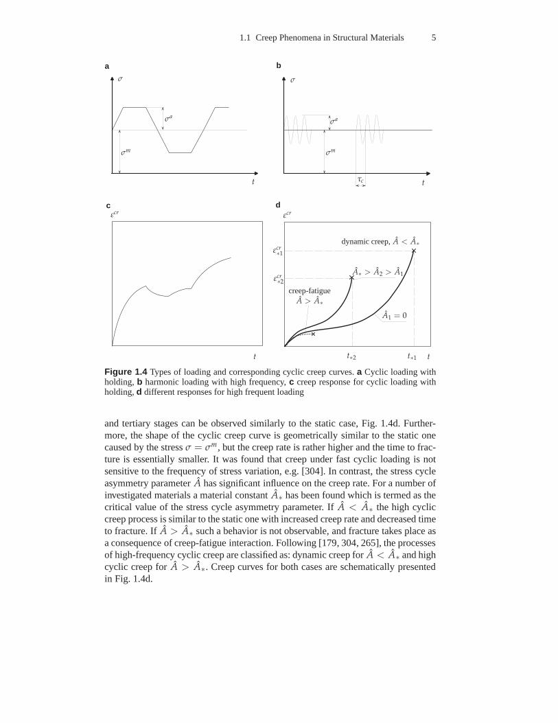
A periodically varied load causes cyclic creep response. The periodic stress canbe characterized by the amplitudeσa, the periodτc and the mean stressσm. Twotypical cases of the periodic loading are presented in Figs 1.4a, b. Let us assumethat the maximum stressσmax = σm + σa is much less than the yield limit of thematerial. Creep behavior for the case of periodic loading with a holding time isschematically illustrated in Fig. 1.4c. Here the mean stress σm, the amplitudeσa,the rate of loading/unloading and the holding time influencethe creep response.The case of harmonic loading is shown in Fig. 1.4b. Such loading is important inthose engineering applications, where technological or operational conditions (non-stationary flow, combustion, acoustic action, etc.) cause the development of forcedvibrations. The harmonic stress variation can be describedas follows
σ = σm(1 + A sin Ωt), A =σa
σm, Ω =
2π
τc= 2π f (1.1.1)
Creep behavior under harmonic loading (1.1.1) with frequencies f > 1 . . . 2 Hz isstudied in [43, 179, 302, 303]. For this cyclic loading condition primary, secondary
1.1 Creep Phenomena in Structural Materials 5
εcr εcr
tt
tt
σ σ
σmσm
σaσa
τc
creep-fatigueA > A∗
dynamic creep,A < A∗
A1 = 0
A∗ > A2 > A1
t∗1t∗2
εcr∗1
εcr∗2
a b
c d
Figure 1.4 Types of loading and corresponding cyclic creep curves.a Cyclic loading withholding,b harmonic loading with high frequency,c creep response for cyclic loading withholding,d different responses for high frequent loading
and tertiary stages can be observed similarly to the static case, Fig. 1.4d. Further-more, the shape of the cyclic creep curve is geometrically similar to the static onecaused by the stressσ = σm, but the creep rate is rather higher and the time to frac-ture is essentially smaller. It was found that creep under fast cyclic loading is notsensitive to the frequency of stress variation, e.g. [304].In contrast, the stress cycleasymmetry parameterA has significant influence on the creep rate. For a number ofinvestigated materials a material constantA∗ has been found which is termed as thecritical value of the stress cycle asymmetry parameter. IfA < A∗ the high cycliccreep process is similar to the static one with increased creep rate and decreased timeto fracture. IfA > A∗ such a behavior is not observable, and fracture takes place asa consequence of creep-fatigue interaction. Following [179, 304, 265], the processesof high-frequency cyclic creep are classified as: dynamic creep forA < A∗ and highcyclic creep forA > A∗. Creep curves for both cases are schematically presentedin Fig. 1.4d.
6 1 Introduction
ε
σ
ε increasing
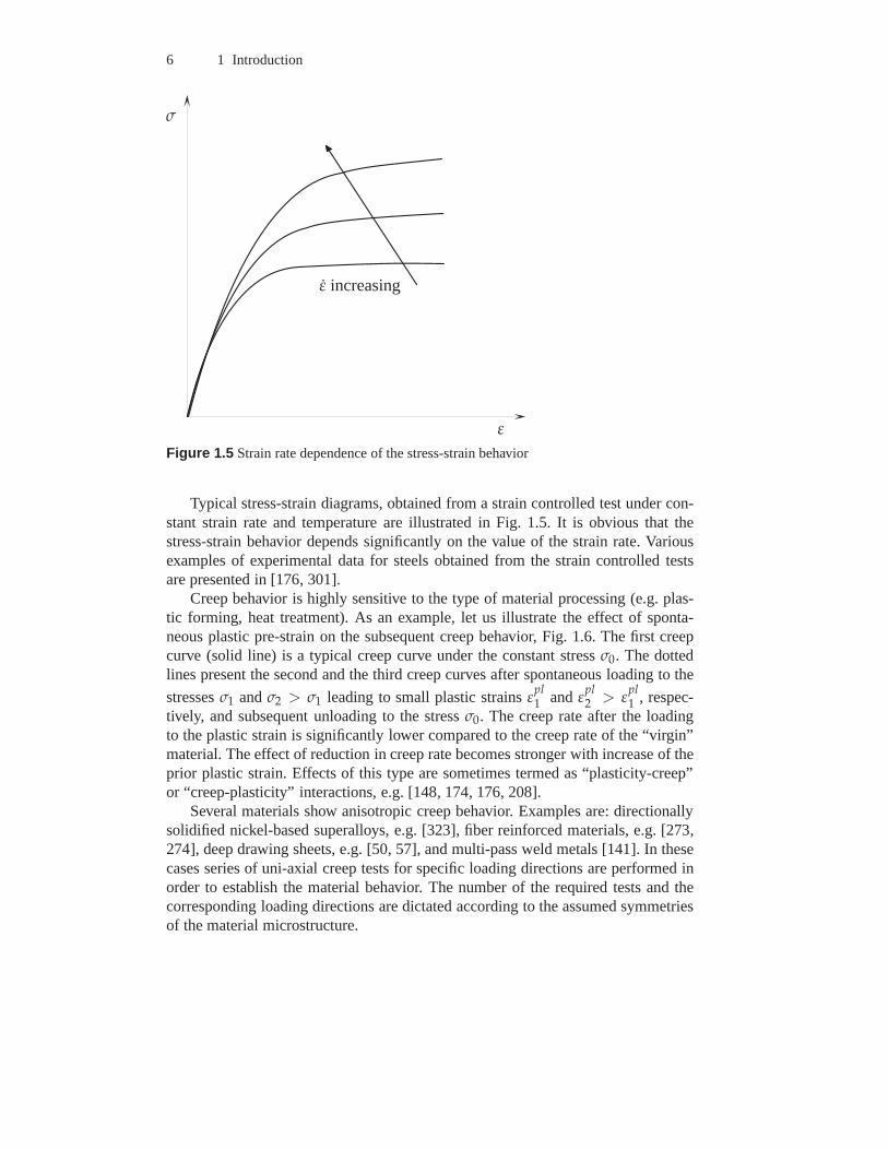
Figure 1.5 Strain rate dependence of the stress-strain behavior
Typical stress-strain diagrams, obtained from a strain controlled test under con-stant strain rate and temperature are illustrated in Fig. 1.5. It is obvious that thestress-strain behavior depends significantly on the value of the strain rate. Variousexamples of experimental data for steels obtained from the strain controlled testsare presented in [176, 301].
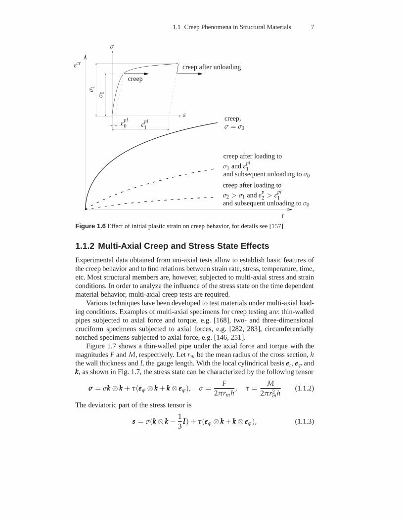
Creep behavior is highly sensitive to the type of material processing (e.g. plas-tic forming, heat treatment). As an example, let us illustrate the effect of sponta-neous plastic pre-strain on the subsequent creep behavior,Fig. 1.6. The first creepcurve (solid line) is a typical creep curve under the constant stressσ0. The dottedlines present the second and the third creep curves after spontaneous loading to the
stressesσ1 andσ2 > σ1 leading to small plastic strainsεpl1 andε
pl2 > ε
pl1 , respec-
tively, and subsequent unloading to the stressσ0. The creep rate after the loadingto the plastic strain is significantly lower compared to the creep rate of the “virgin”material. The effect of reduction in creep rate becomes stronger with increase of theprior plastic strain. Effects of this type are sometimes termed as “plasticity-creep”or “creep-plasticity” interactions, e.g. [148, 174, 176, 208].
Several materials show anisotropic creep behavior. Examples are: directionallysolidified nickel-based superalloys, e.g. [323], fiber reinforced materials, e.g. [273,274], deep drawing sheets, e.g. [50, 57], and multi-pass weld metals [141]. In thesecases series of uni-axial creep tests for specific loading directions are performed inorder to establish the material behavior. The number of the required tests and thecorresponding loading directions are dictated according to the assumed symmetriesof the material microstructure.
1.1 Creep Phenomena in Structural Materials 7
replacements
t
εcr
ε
σ
εpl0 ε
pl1
σ 0
σ 1
creep
creep after unloading
creep,σ = σ0
creep after loading to
σ1 andεpl1
and subsequent unloading toσ0
creep after loading to
σ2 > σ1 andεp2 > ε
pl1
and subsequent unloading toσ0
Figure 1.6 Effect of initial plastic strain on creep behavior, for details see [157]
1.1.2 Multi-Axial Creep and Stress State Effects
Experimental data obtained from uni-axial tests allow to establish basic features ofthe creep behavior and to find relations between strain rate,stress, temperature, time,etc. Most structural members are, however, subjected to multi-axial stress and strainconditions. In order to analyze the influence of the stress state on the time dependentmaterial behavior, multi-axial creep tests are required.
Various techniques have been developed to test materials under multi-axial load-ing conditions. Examples of multi-axial specimens for creep testing are: thin-walledpipes subjected to axial force and torque, e.g. [168], two- and three-dimensionalcruciform specimens subjected to axial forces, e.g. [282, 283], circumferentiallynotched specimens subjected to axial force, e.g. [146, 251].
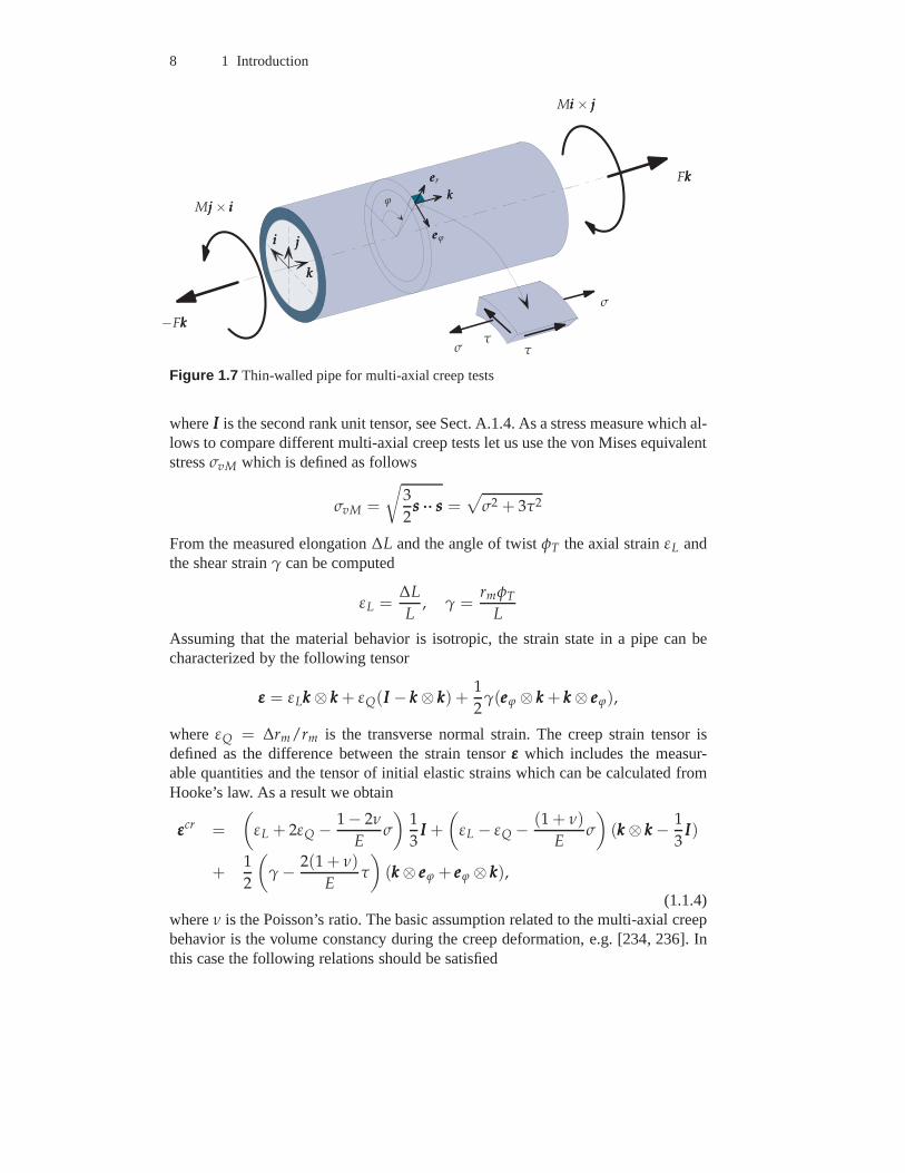
Figure 1.7 shows a thin-walled pipe under the axial force andtorque with themagnitudesF andM, respectively. Letrm be the mean radius of the cross section,hthe wall thickness andL the gauge length. With the local cylindrical basiseeer, eeeϕ andkkk, as shown in Fig. 1.7, the stress state can be characterized by the following tensor
σσσ = σkkk ⊗ kkk + τ(eeeϕ ⊗ kkk + kkk ⊗ eeeϕ), σ =F
2πrmh, τ =
M
2πr2mh
(1.1.2)
The deviatoric part of the stress tensor is
sss = σ(kkk ⊗ kkk − 1
3III) + τ(eeeϕ ⊗ kkk + kkk ⊗ eeeϕ), (1.1.3)
8 1 Introduction
iii jjj
kkk
−Fkkk
Fkkk
Mjjj × iii
Miii × jjj
σ
σ ττ
eeeϕ
eeer
kkkϕ
Figure 1.7 Thin-walled pipe for multi-axial creep tests
whereIII is the second rank unit tensor, see Sect. A.1.4. As a stress measure which al-lows to compare different multi-axial creep tests let us usethe von Mises equivalentstressσvM which is defined as follows
σvM =
√
3
2sss ······ sss =
√
σ2 + 3τ2
From the measured elongation∆L and the angle of twistφT the axial strainεL andthe shear strainγ can be computed
εL =∆L
L, γ =
rmφT
L
Assuming that the material behavior is isotropic, the strain state in a pipe can becharacterized by the following tensor
εεε = εLkkk ⊗ kkk + εQ(III − kkk ⊗ kkk) +1
2γ(eeeϕ ⊗ kkk + kkk ⊗ eeeϕ),
whereεQ = ∆rm/rm is the transverse normal strain. The creep strain tensor isdefined as the difference between the strain tensorεεε which includes the measur-able quantities and the tensor of initial elastic strains which can be calculated fromHooke’s law. As a result we obtain
εεεcr =
(
εL + 2εQ − 1 − 2ν
Eσ
)
1
3III +
(
εL − εQ − (1 + ν)
Eσ
)
(kkk ⊗ kkk − 1
3III)
+1
2
(
γ − 2(1 + ν)
Eτ
)
(kkk ⊗ eeeϕ + eeeϕ ⊗ kkk),
(1.1.4)whereν is the Poisson’s ratio. The basic assumption related to the multi-axial creepbehavior is the volume constancy during the creep deformation, e.g. [234, 236]. Inthis case the following relations should be satisfied
1.1 Creep Phenomena in Structural Materials 9
tr εεε = tr εεεel ⇒ εL + 2εQ =1 − 2ν
Eσ
From (1.1.4) follows
εεεcr =3
2
(
εL −1
Eσ
)
(kkk ⊗ kkk − 1
3III) +
1
2
(
γ − 2(1 + ν)
Eτ
)
(kkk ⊗ eeeϕ + eeeϕ ⊗ kkk)
Under the condition of stationary loading the creep rate tensor is
εεε = εεεcr =3
2εL(kkk ⊗ kkk − 1
3III) +
1
2γ(kkk ⊗ eeeϕ + eeeϕ ⊗ kkk) (1.1.5)
The von Mises equivalent creep rate is defined by
εvM =
√
2
3εεε ······ εεε =
√
ε2L +
1
3γ2
The results of creep tests on tubes are usually presented as:strainsεL andγ vs. timecurves, e.g. [136, 148, 157], creep strains
εcrL = εL −
σ
E, γcr = γ − 2(1 + ν)
Eτ
vs. time curves, e.g [218, 248, 238], von Mises equivalent creep strain
εcrvM =
√
2
3εεεcr ······ εεεcr =
√
(εcrL )2 +
1
3(γcr)2
vs. time curves, e.g. [168, 170], and the so-called specific dissipation work
q(t) =
t∫
0
εεε······ sssdt =
t∫
0
(εLσ + γτ)dt
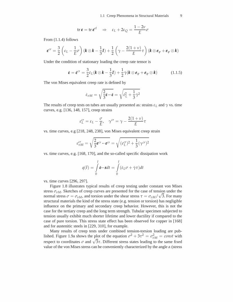
vs. time curves [296, 297].Figure 1.8 illustrates typical results of creep testing under constant von Mises
stressσvM. Sketches of creep curves are presented for the case of tension under thenormal stressσ = σvM, and torsion under the shear stressτ = σvM/
√3. For many
structural materials the kind of the stress state (e.g. tension or torsion) has negligibleinfluence on the primary and secondary creep behavior. However, this is not thecase for the tertiary creep and the long term strength. Tubular specimen subjected totension usually exhibit much shorter lifetime and lower ductility if compared to thecase of pure torsion. This stress state effect has been observed for copper in [168]and for austenitic steels in [229, 310], for example.
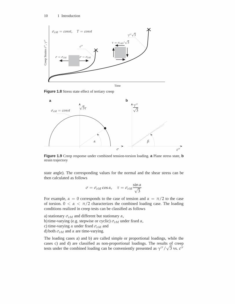
Many results of creep tests under combined tension-torsionloading are pub-lished. Figure 1.9a shows the plot of the equationσ2 + 3τ2 = σ2
vM = const withrespect to coordinatesσ and
√3τ. Different stress states leading to the same fixed
value of the von Mises stress can be conveniently characterized by the angleα (stress
10 1 Introduction
Time
Cre
epS
trai
nsεcr
,γcr
σ = σvMσ = σvM
τ = σvM/√
3
σvM = const, T = const
εcr
γcr√
3
Figure 1.8 Stress state effect of tertiary creep
σ
√3τ
σvM = const
α
εcr
γcr
√3
β
a b
Figure 1.9 Creep response under combined tension-torsion loading.a Plane stress state,bstrain trajectory
state angle). The corresponding values for the normal and the shear stress can bethen calculated as follows
σ = σvM cos α, τ = σvMsin α√
3
For example,α = 0 corresponds to the case of tension andα = π/2 to the caseof torsion.0 < α < π/2 characterizes the combined loading case. The loadingconditions realized in creep tests can be classified as follows
a) stationaryσvM and different but stationaryα,b) time-varying (e.g. stepwise or cyclic)σvM under fixedα,c) time-varyingα under fixedσvM andd) bothσvM andα are time-varying.
The loading cases a) and b) are called simple or proportionalloadings, while thecases c) and d) are classified as non-proportional loadings.The results of creeptests under the combined loading can be conveniently presented asγcr/
√3 vs. εcr
1.2 Creep in Engineering Structures 11
curves (so-called strain trajectories), e.g. [218, 228]. Asketch of such a curve forthe loading case a) is presented in Fig. 1.9b. For many metalsand alloys, e.g. [218,228, 245], the direction of the strain trajectory characterized by the angelβ, Fig.1.9b, coincides with the direction of the applied stress state, characterized by theangleα. According to this result one can assume that the creep rate tensor is coaxialand collinear with the stress deviator, i.e.εεε = λsss. Taking into account (1.1.2) and(1.1.5) the following relations can be obtained
3
2εL = λσ,
1
2γ = λτ ⇒ εL
γ/√
3=
σ√3τ
In many cases, experimental results show that the above relations are well satisfied,e.g. [136, 218, 228, 245].
Non-coincidence of the strain-trajectory and the stress state angles indicates theanisotropy of the creep behavior. Anisotropic creep may be caused either by theinitial anisotropy of the material microstructure as a result of material processingor by the anisotropy induced during the creep process. Examples for anisotropictension-torsion creep are presented for a directionally solidified nickel-based su-peralloy in [239] and for a fiber-reinforced material in [273, 274]. The trajecto-ries of creep strains presented in [157] for austenitic steel tubes demonstrate thatinitial small plastic pre-strain causes the anisotropy of subsequent creep behavior.The deformation induced anisotropy may be observed in creeptests under non-proportional loading conditions. The effects of the induced anisotropy are usuallyrelated to anisotropic hardening, e.g. [245, 157, 228], anddamage processes, e.g.[218].
Another stress state effect is the different creep behaviorunder tensile and com-pressive loadings. Examples are presented for several alloys in [106, 195, 301, 339],for polymers in [187], and for ceramics in [254]. Experimental results show that forthe same value of stress in tension and compression, the value of the creep rateunder tension is significantly greater than the corresponding absolute value undercompression. This effect indicates that besides the von Mises equivalent stress, ad-ditional characteristics of the stress state (e.g. the meanstress) may influence thecreep process.
1.2 Creep in Engineering Structures
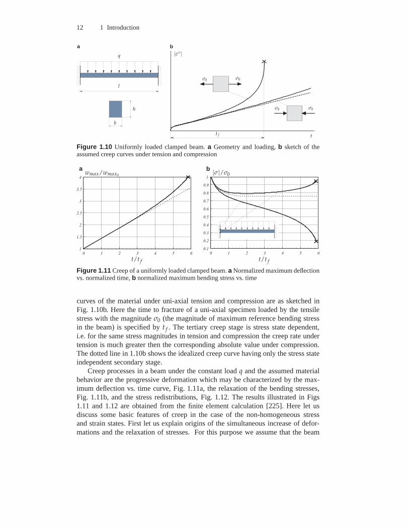
Creep in structures is a variety of time dependent changes ofstrain and stress statesincluding progressive deformations, relaxation and redistribution of stresses, localreduction of the material strength. To illustrate these processes let us consider abeam with a rectangular cross section. We assume that the beam is heated up toa certain temperature, clamped at the ends and uniformly loaded as shown in Fig.1.10a. The loading is moderate leading to spontaneous elastic deformation of thebeam. Let the maximum deflection of the beam in the reference “elastic” state bew0 and the maximum bending stress beσ0. Furthermore, let us assume that creep
12 1 Introduction
t
|εcr|
σ0σ0
σ0σ0
t f
l
q
b
h
a b
Figure 1.10 Uniformly loaded clamped beam.a Geometry and loading,b sketch of theassumed creep curves under tension and compression
0 1 2 3 4 5 60 . 1
0 . 2
0 . 3
0 . 4
0 . 5
0 . 6
0 . 7
0 . 8
0 . 9
1
0 1 2 3 4 5 61
1 . 5
2
2 . 5
3
3 . 5
4
t/t ft/t f
wmax/wmax0|σ|/σ0
a b
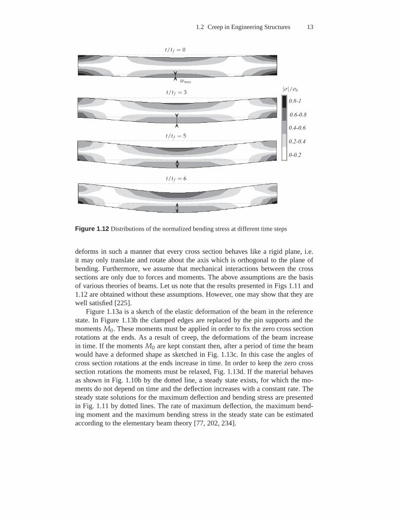
Figure 1.11 Creep of a uniformly loaded clamped beam.a Normalized maximum deflectionvs. normalized time,b normalized maximum bending stress vs. time
curves of the material under uni-axial tension and compression are as sketched inFig. 1.10b. Here the time to fracture of a uni-axial specimenloaded by the tensilestress with the magnitudeσ0 (the magnitude of maximum reference bending stressin the beam) is specified byt f . The tertiary creep stage is stress state dependent,i.e. for the same stress magnitudes in tension and compression the creep rate undertension is much greater then the corresponding absolute value under compression.The dotted line in 1.10b shows the idealized creep curve having only the stress stateindependent secondary stage.
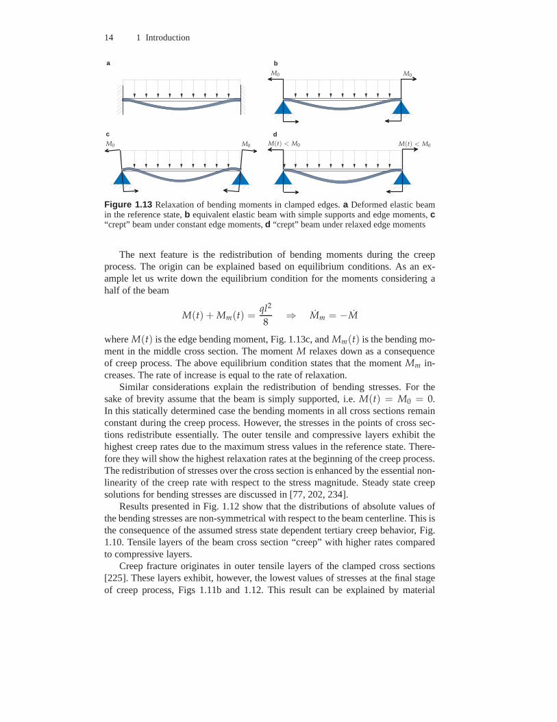
Creep processes in a beam under the constant loadq and the assumed materialbehavior are the progressive deformation which may be characterized by the max-imum deflection vs. time curve, Fig. 1.11a, the relaxation ofthe bending stresses,Fig. 1.11b, and the stress redistributions, Fig. 1.12. The results illustrated in Figs1.11 and 1.12 are obtained from the finite element calculation [225]. Here let usdiscuss some basic features of creep in the case of the non-homogeneous stressand strain states. First let us explain origins of the simultaneous increase of defor-mations and the relaxation of stresses. For this purpose we assume that the beam
1.2 Creep in Engineering Structures 13
0 . 8 - 1
0 - 0 . 2
0 . 2 - 0 . 4
0 . 4 - 0 . 6
0 . 6 - 0 . 8
|σ|/σ0
t/t f = 0
t/t f = 3
t/t f = 5
t/t f = 6
wmax
Figure 1.12 Distributions of the normalized bending stress at different time steps
deforms in such a manner that every cross section behaves like a rigid plane, i.e.it may only translate and rotate about the axis which is orthogonal to the plane ofbending. Furthermore, we assume that mechanical interactions between the crosssections are only due to forces and moments. The above assumptions are the basisof various theories of beams. Let us note that the results presented in Figs 1.11 and1.12 are obtained without these assumptions. However, one may show that they arewell satisfied [225].
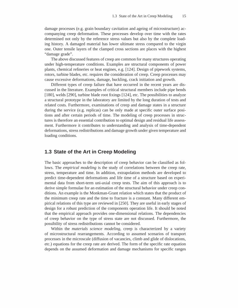
Figure 1.13a is a sketch of the elastic deformation of the beam in the referencestate. In Figure 1.13b the clamped edges are replaced by the pin supports and themomentsM0. These moments must be applied in order to fix the zero cross sectionrotations at the ends. As a result of creep, the deformationsof the beam increasein time. If the momentsM0 are kept constant then, after a period of time the beamwould have a deformed shape as sketched in Fig. 1.13c. In thiscase the angles ofcross section rotations at the ends increase in time. In order to keep the zero crosssection rotations the moments must be relaxed, Fig. 1.13d. If the material behavesas shown in Fig. 1.10b by the dotted line, a steady state exists, for which the mo-ments do not depend on time and the deflection increases with aconstant rate. Thesteady state solutions for the maximum deflection and bending stress are presentedin Fig. 1.11 by dotted lines. The rate of maximum deflection, the maximum bend-ing moment and the maximum bending stress in the steady statecan be estimatedaccording to the elementary beam theory [77, 202, 234].
14 1 Introduction
M0
M0M0
M0 M(t) < M0M(t) < M0
a b
c d
Figure 1.13 Relaxation of bending moments in clamped edges.a Deformed elastic beamin the reference state,b equivalent elastic beam with simple supports and edge moments,c“crept” beam under constant edge moments,d “crept” beam under relaxed edge moments
The next feature is the redistribution of bending moments during the creepprocess. The origin can be explained based on equilibrium conditions. As an ex-ample let us write down the equilibrium condition for the moments considering ahalf of the beam
M(t) + Mm(t) =ql2
8⇒ Mm = −M
whereM(t) is the edge bending moment, Fig. 1.13c, andMm(t) is the bending mo-ment in the middle cross section. The momentM relaxes down as a consequenceof creep process. The above equilibrium condition states that the momentMm in-creases. The rate of increase is equal to the rate of relaxation.
Similar considerations explain the redistribution of bending stresses. For thesake of brevity assume that the beam is simply supported, i.e. M(t) = M0 = 0.In this statically determined case the bending moments in all cross sections remainconstant during the creep process. However, the stresses inthe points of cross sec-tions redistribute essentially. The outer tensile and compressive layers exhibit thehighest creep rates due to the maximum stress values in the reference state. There-fore they will show the highest relaxation rates at the beginning of the creep process.The redistribution of stresses over the cross section is enhanced by the essential non-linearity of the creep rate with respect to the stress magnitude. Steady state creepsolutions for bending stresses are discussed in [77, 202, 234].
Results presented in Fig. 1.12 show that the distributions of absolute values ofthe bending stresses are non-symmetrical with respect to the beam centerline. This isthe consequence of the assumed stress state dependent tertiary creep behavior, Fig.1.10. Tensile layers of the beam cross section “creep” with higher rates comparedto compressive layers.
Creep fracture originates in outer tensile layers of the clamped cross sections[225]. These layers exhibit, however, the lowest values of stresses at the final stageof creep process, Figs 1.11b and 1.12. This result can be explained by material
1.3 State of the Art in Creep Modeling 15
damage processes (e.g. grain boundary cavitation and ageing of microstructure) ac-companying creep deformation. These processes develop over time with the ratesdetermined not only by the reference stress values but also by the complete load-ing history. A damaged material has lower ultimate stress compared to the virginone. Outer tensile layers of the clamped cross sections are places with the highest“damage grade”.
The above discussed features of creep are common for many structures operatingunder high-temperature conditions. Examples are structural components of powerplants, chemical refineries or heat engines, e.g. [124]. Design of pipework systems,rotors, turbine blades, etc. requires the consideration ofcreep. Creep processes maycause excessive deformations, damage, buckling, crack initiation and growth.
Different types of creep failure that have occurred in the recent years are dis-cussed in the literature. Examples of critical structural members include pipe bends[180], welds [290], turbine blade root fixings [124], etc. The possibilities to analyzea structural prototype in the laboratory are limited by the long duration of tests andrelated costs. Furthermore, examinations of creep and damage states in a structureduring the service (e.g. replicas) can be only made at specific outer surface posi-tions and after certain periods of time. The modeling of creep processes in struc-tures is therefore an essential contribution to optimal design and residual life assess-ment. Furthermore it contributes to understanding and analysis of time-dependentdeformations, stress redistributions and damage growth under given temperature andloading conditions.
1.3 State of the Art in Creep Modeling
The basic approaches to the description of creep behavior can be classified as fol-lows. Theempirical modeling is the study of correlations between the creep rate,stress, temperature and time. In addition, extrapolation methods are developed topredict time-dependent deformations and life time of a structure based on experi-mental data from short-term uni-axial creep tests. The aim of this approach is toderive simple formulae for an estimation of the structural behavior under creep con-ditions. An example is the Monkman-Grant relation which states that the product ofthe minimum creep rate and the time to fracture is a constant.Many different em-pirical relations of this type are reviewed in [250]. They are useful in early stages ofdesign for a robust prediction of the components operation life. It should be notedthat the empirical approach provides one-dimensional relations. The dependenciesof creep behavior on the type of stress state are not discussed. Furthermore, thepossibility of stress redistributions cannot be considered.
Within the materials science modeling, creep is characterized by a varietyof microstructural rearrangements. According to assumed scenarios of transportprocesses in the microscale (diffusion of vacancies, climband glide of dislocations,etc.) equations for the creep rate are derived. The form of the specific rate equationdepends on the assumed deformation and damage mechanisms for specific ranges
16 1 Introduction
of stress and temperature, e.g. [117]. Many diverse equations of this type are re-viewed in [116, 156, 222]. In addition, kinetic equations for internal state variablesare discussed. Examples for these variables include dislocation density, [110], inter-nal (back) stress, e.g. [116], and various damage parameters associated with ageingand cavitation processes, [101]. The aim of this approach isto provide correlationsbetween quantities characterizing the type of microstructure and processing (grainsize, types of alloying and hardening, etc.) and quantitiescharacterizing the mater-ial behavior, e.g. the creep rate. Furthermore, the mechanisms based classification ofdifferent forms of creep equations including different stress and temperature func-tions is helpful in the structural analysis. However, the models proposed within thematerials science are usually one-dimensional and operatewith scalar-valued quan-tities like magnitudes of stress and strain rates.
Themicromechanical models deal with discrete simulations of material behav-ior for a representative volume element with geometricallyidealized microstructure.Simplifying assumptions are made for the behavior of constituents and their interac-tions, for the type of the representative volume element andfor the exerted bound-ary conditions. Examples include numerical simulations ofvoid growth in a powerlaw creeping matrix material, e.g. [315, 318], crack propagation through a powerlaw creeping multi-grain model, e.g. [241, 317], stress redistributions between con-stituents in a creeping binary medium, e.g. [226]. Micromechanical models con-tribute to understanding creep and damage processes in heterogeneous systems.With respect to engineering applications the micromechanical approach suffers,however, from significant limitations. One of them is that a typical high-temperaturestructural material, for example steel, has a complex composition including dislo-cation structures, grain boundaries, dispersion particles, precipitates, etc. A reliablemicromechanical description of creep in a structural steelwould therefore require arather complex model of a multi-phase medium with many evolving and interactingconstituents.
The objective ofcontinuum mechanics modeling is to investigate creep in ide-alized three-dimensional solids. The idealization is related to the hypothesis of acontinuum, e.g. [131]. The approach is based on balance equations formulated formaterial volume elements and assumptions regarding the kinematics of deforma-tion and motion. Creep behavior is described by means of constitutive equationswhich relate deformation processes and stresses. Details of topological changes ofmicrostructure like subgrain size or mean radius of carbideprecipitates are not con-sidered. The processes associated with these changes like hardening, recovery, age-ing and damage can be taken into account by means of hidden or internal state vari-ables and corresponding evolution equations, [58, 185, 265, 291]. Creep constitutiveequations with internal state variables can be applied to structural analysis. Variousmodels and methods recently developed within the mechanicsof structures can beextended to the solution of creep problems. Examples are theories of rods, plates andshells as well as direct variational methods, e.g. [6, 58, 77, 202, 255, 292]. Numeri-cal solutions by the finite element method combined with various time step integra-tion techniques allow to simulate time dependent structural behavior up to critical
1.4 Scope and Outline 17
state of failure. Examples of recent studies include circumferentially notched bars[133], pipe weldments [137] and thin-walled tubes [177]. Inthese investigationsqualitative agreements between the theory and experimentscarried out on modelstructures have been established. Constitutive equationswith internal state variableshave been found to be mostly suited for the creep analysis of structures [137]. How-ever, it should be noted that this approach requires numerous experimental data ofcreep for structural materials over a wide range of stress and temperature as well asdifferent stress states.
1.4 Scope and Outline
This work is a contribution to the continuum mechanics modeling of creep withthe aim of structural analysis. This type of modeling is related to the fields “creepmechanics” [58, 235] and “creep continuum damage mechanics” [135] and requiresthe following steps [77, 139, 234]
– formulation of a constitutive model including constitutive and evolution equationsto reflect basic features of creep behavior of a structural material under multi-axialstress states,
– identification of material constants in constitutive and evolution equations basedon experimental data of creep and long-term strength,
– application of a structural mechanics model by taking into account creepprocesses and stress state effects,
– formulation of an initial-boundary value problem based on the constitutive andstructural mechanics models,
– development of numerical solution procedures and– verification of results
The text is organized as follows. Chapter 2 provides an overview of constitutivemodels that describe creep processes under multi-axial stress states. The startingpoint of the engineering creep theory is the introduction ofthe inelastic strain, thecreep potential, the flow rule, the equivalent stress and internal state variables. Con-stitutive models of isotropic secondary creep based on the von Mises-Odqvist creeppotential are introduced. To account for stress state effects creep potentials that in-clude three invariants of the stress tensor are discussed. Consideration of materialsymmetries provide restrictions for the creep potential. Anovel direct approach tofind scalar valued arguments of the creep potential for the given group of mater-ial symmetries is proposed. Transverse isotropy and orthotropic symmetry are twoimportant types of symmetries in the creep mechanics [58]. For these two cases ap-propriate invariants of the stress tensor, equivalent stress and strain expressions aswell as constitutive equations are derived.
Further extensions of the classical creep theory are related to processes accom-panying creep deformation. Primary creep and transient creep effects can be de-scribed by the introduction of hardening state variables. The time and strain hard-ening models as well as the back stress concept are examined as they predict multi-
18 1 Introduction
axial creep behavior. Tertiary creep and long term strengthcan be characterized bythe introduction of damage state variables. A systematic review of different typesof constitutive equations with damage variables and corresponding evolution equa-tions is presented. Stress state effects and damage inducedanisotropy are discussedin detail.
Chapter 3 deals with the application of constitutive modelsto the description ofcreep for several structural materials. Constitutive and evolution equations, responsefunctions and material constants are presented according to recently published ex-perimental data. Furthermore a new model for anisotropic creep in a multi-pass weldmetal is presented.
In Chapter 4 we discuss structural mechanics problems. We start with a sum-mary of governing equations describing creep in three-dimensional solids. Severalsimplifying assumptions are made in order to illustrate thebasic ideas of initial-boundary value problems, direct variational methods and time step algorithms. Thenvarious structural mechanics models of beams, plates and shells are reviewed andevaluated in the context of their applicability to creep problems. An emphasis isplaced on effects of transverse shear deformation, boundary layers and geometricalnonlinearities.
A model with a scalar damage variable is incorporated into the ANSYS finite el-ement code by means of a user defined material subroutine. To verify the developedsubroutine several benchmark problems are presented. For these problems specialnumerical solutions based on the Ritz method are obtained. Finite element solutionsfor the same problems are performed to illustrate that the subroutine is correctlycoded and implemented. Furthermore these benchmarks are used to study the ap-plicability of the developed subroutine over a wide range ofelement types includingshell and solid elements. Based on several examples, the influence of the mesh sizeon the accuracy of solutions is demonstrated. Finally an example for a spatial steampipeline is presented. Results are compared with the data from engineering practicediscussed in the literature.
Appendix A is a summary of the direct tensor notation and basic tensor opera-tions used throughout the text. This notation has an advantage of a clear, compactand coordinate free representation of constitutive modelsand initial-boundary valueproblems. The theory of anisotropic tensor functions and invariants is discussed indetail. A novel approach to derive the basic set of functionally independent invari-ants for vectors and second rank tensors for the given symmetry group is presented.The invariants are found as integrals of a generic partial differential equation (basicequation for invariants).
2 Constitutive Models of Creep
Analysis of creep in engineering structures requires the formulation and the solutionof an initial-boundary value problem including the balanceequations and the consti-tutive assumptions. Equations describing the kinematics of three-dimensional solidsas well as balance equations of mechanics of media are presented in monographsand textbooks on continuum mechanics, e.g. [29, 35, 44, 57, 108, 131, 178, 199]. Inwhat follows we discuss constitutive equations for the description of creep behaviorin three-dimensional solids.
The starting point of the engineering creep theory is the introduction of the in-elastic strain, the creep potential, the flow rule, the equivalent stress and internalstate variables, Sect. 2.1. In Sect. 2.2 we discuss constitutive models of secondarycreep. We start with the von Mises-Odqvist creep potential and the flow rule widelyused in the creep mechanics. To account for stress state effects creep potentialsthat include three invariants of the stress tensor are introduced. Consideration ofmaterial symmetries provide restrictions for the creep potential. A novel direct ap-proach to find scalar valued arguments of the creep potentialfor the given group ofmaterial symmetries is proposed. For several cases of material symmetry appropri-ate invariants of the stress tensor, equivalent stress and strain expressions as wellas constitutive equations for anisotropic creep are derived. In Sect. 2.3 we reviewexperimental foundations and models of transient creep behavior under differentmulti-axial loading conditions. Section 2.4 is devoted to the description of tertiarycreep under multi-axial stress states. Various models within the framework of con-tinuum damage mechanics are discussed.
All equations are presented in the direct tensor notation. This notation guaran-tees the invariance with respect to the choice of the coordinate system and has theadvantage of clear and compact representation of constitutive assumptions, partic-ularly in the case of anisotropic creep. The basic rules of the direct tensor calculusas well as some new results for basic sets of invariants with respect to differentsymmetry classes are presented in Appendix A.
2.1 General Remarks
The modeling of creep under multi-axial stress states is thekey step in the adequateprediction of the long-term structural behavior. Such a modeling requires the in-troduction of tensors of stress, strain, strain rate and corresponding inelastic parts.
20 2 Constitutive Models of Creep
Usually, they are discussed within the framework of continuum mechanics start-ing from fundamental balance equations. One of the most important and funda-mental questions is that of the definition (or even the existence) of a measure ofthe inelastic strain and the decomposition of the total strain into elastic and irre-versible parts within the material description. From the theoretical point of viewthis is still a subject of many discussions within the non-linear continuum mechan-ics, e.g. [45, 46, 223, 246].
In engineering mechanics, these concepts are often introduced based on intu-itive assumptions, available experimental data and applications. Therefore, a lot offormulations of multi-axial creep equations can be found inthe literature. In whatfollows some of them will be discussed. First let us recall several assumptions usu-ally made in the creep mechanics [58, 235].
The assumption of infinitesimal strains allows to neglect the difference betweenthe true stresses and strains and the engineering stresses and strains. According tothe continuum mechanics there are no differences between the Eulerian and theLagrangian approaches within the material description. Creep equations in the geo-metrical non-linear case (finite strains) are discussed in the monograph [67], forexample. Finite strain equations based on rheological models are presented in themonographs [175, 246]. The linearized equations of creep continuum mechanicscan be used in the majority of engineering applications because structures are usu-ally designed such that the displacements and strains arising as a consequence of theapplied loading do not exceed the prescribed small values. The exception is the caseof thin-walled shells, where geometrical non-linearitiesmust be considered even ifstrains are infinitesimal, see Sect. 4.4.
The assumption of the classical non-polar continuum restricts the class of mate-rials. The equations of motion within the continuum mechanics include the balanceof momentum and the balance of angular momentum, e.g. [108].These equations in-troduce the stress and the moment stress tensors. Polar materials are those which arecharacterized by constitutive equations with respect to both tensors (in general, theyare non-symmetric). In addition, the rotation degrees of freedom, i.e. the rotationtensor and the angular velocity, are introduced as independent quantities. Models ofpolar media found application to granular or porous materials [97, 104, 214], fibersuspensions [22, 109], or other media with changing microstructure. At present, themoment stress tensor and the anti-symmetric part of the stress tensor are not con-sidered in the engineering creep theories. The reason for this is the higher ordercomplexity of the models and as a consequence increased effort for the identifica-tion of material characteristics.
The assumption of isothermal conditions makes it possible to decouple the ther-mal and the mechanical problem. Furthermore, heat transferproblems are not con-sidered. The influence of the constant temperature on the creep rate is describedby an Arrhenius function, see Sect. 2.2.3. Coupled thermo-mechanical problems ofcreep and damage are discussed in [291], where the influence of creep cavitation onthermal conductivity is considered.
2.1 General Remarks 21
In this chapter we shall use the following notation. Letσσσ be the Cauchy stresstensor andεεε be the tensor of infinitesimal strains as they are defined in [29, 57, 199],among others. Let the symmetric second rank tensorεεεcr be the tensor of the rateof infinitesimal inelastic strains induced by the creep process. For the infinitesimalstrains one can assume the additive split of the total strainrate into elastic and creepparts, i.e.εεε = εεεel + εεεcr. The constitutive equation relating the stress tensor andthe elastic part of the strain tensor can be formulated according to the generalizedHooke’s law [29, 55, 126, 199] and will be introduced later. Creep deformation isaccompanied by various microstructural changes having different influences on thestrain rate. The current state of the material microstructure is determined by theentire previous history of the creep process. It can be characterized by a set of addi-tional field variables termed as internal or hidden state variables. In this chapter weshall discuss internal state variables characterizing thestates of hardening/recoveryand damage. In order to distinguish between the hardening and damage mechanismswe shall specify the “internal hardening variables” byHi and the “internal damagevariables” byωj. The number of such variables and the corresponding evolutionequations (ordinary differential equations with respect to the time variable) is dic-tated by the knowledge of creep-damage mechanisms for a specified metal or alloy,the availability of experimental data on creep and long termstrength as well as thetype of the structural analysis application. In some cases the internal state variablesmust be introduced as tensors of different rank in order to include effects of thedeformation or damage induced anisotropy.
Constitutive equations of multi-axial creep are usually based on the concept ofthe creep potential and the flow rule. The associated flow rulehas the origin in theengineering theory of plasticity. The basic assumptions ofthis theory are:
– The existence of a yield condition (creep condition, see [55], for example) ex-pressed by the equationF(σσσ) = 0, whereF is a scalar valued function. In thegeneral case one can presume thatF depends not only on the stress tensor butalso on the internal state variables and the temperature [202, 265], i.e. the yieldcondition has a form
F(σσσ, Hi, ωj, T) = 0, i = 1, . . . , n, j = 1, . . . , m (2.1.1)
– The existence of a flow potential as a function of the stress tensorΦ(σσσ).
The flow rule (sometimes called the normality rule) is the following assumption forthe inelastic strain rate tensor
εεεin = η∂Φ
∂σσσ, (2.1.2)
whereη is a scalar factor. In the special case that the flow potentialcoincides withthe yield function i.e.Φ = F (2.1.2) represents the associated flow rule. With respectto the variation of the stress tensorδσσσ one distinguishes between the cases of elasticstate, unloading from an elastic-plastic state, neutral loading and loading, i.e.
22 2 Constitutive Models of Creep
F(σσσ) < 0, elastic state
F(σσσ) = 0, and δF = δσσσ ······ ∂F
∂σσσ< 0 unloading
F(σσσ) = 0, and δF = δσσσ ······ ∂F
∂σσσ= 0 neutral loading
F(σσσ) = 0, and δF = δσσσ ······ ∂F
∂σσσ> 0 loading
For work hardening materialsη > 0 is set in the case of loading/neutral loading,otherwiseη = 0, see e.g. [201]. Further details of the flow theory as well as differentarguments leading to (2.1.2) can be found in textbooks on theory of plasticity, e.g.[138, 151, 153, 161, 201, 206, 292].
Within the creep mechanics the flow theory is usually appliedwithout the con-cept of the yield stress or yield condition. This is motivated by the fact that creepis a thermally activated process and the material starts to creep even under low andmoderate stresses lying below the yield limit. Furthermore, at high temperatures0.5Tm < T < 0.7Tm the main creep mechanism for metals and alloys is the dif-fusion of vacancies, e.g. [117]. Under this condition the existence of a yield or acreep limit cannot be verified experimentally. In [185], p.278 it is stated that “theconcept of a loading surface and the loading-unloading criterion which was used inplasticity is no longer necessary”. In monographs [55, 58, 201, 202, 250] the flowrule is applied as follows
εεεcr = η∂Φ
∂σσσ, η > 0 (2.1.3)
Equation (2.1.3) states the “normality” of the creep rate tensor to the surfacesΦ(σσσ) = const. The scalar factorη is determined according to the hypothesis ofthe equivalence of the dissipation power [2, 58]. The dissipation power is definedby P = εεεcr ······ σσσ. It is assumed thatP = εcr
eqσeq, whereεcreq is an equivalent creep
rate andσeq is an equivalent stress. The equivalent measures of stress and creep rateare convenient to compare experimental data under different stress states (see Sect.1.1.2). From the above hypothesis follows
η =P
∂Φ
∂σσσ······ σσσ
=εcr
eqσeq
∂Φ
∂σσσ······ σσσ
(2.1.4)
The equivalent creep rate is defined as a function of the equivalent stress accordingto the experimental data for uni-axial creep as well as creepmechanisms operatingfor the given stress range. An example is the power law stressfunction
εcreq(σeq) = aσn
eq (2.1.5)
Another form of the flow rule without the yield condition has been proposed byOdqvist, [234, 236]. The steady state creep theory by Odqvist, see [234], p.21 isbased on the variational equationδW = δσσσ ······ εεεcr leading to the flow rule
2.1 General Remarks 23
εεεcr =∂W
∂σσσ, (2.1.6)
where the scalar valued functionW(σσσ) plays the role of the creep potential1. In or-der to specify the creep potential, the equivalent stressσeq(σσσ) is introduced. Takinginto account thatW(σσσ) = W(σeq(σσσ)) the flow rule (2.1.6) yields
εεεcr =∂W
∂σeq
∂σeq
∂σσσ= εcr
eq
∂σeq
∂σσσ, εcr
eq ≡∂W
∂σeq(2.1.7)
The creep potentialW(σeq) is defined according to experimental data of creep underuni-axial stress state for the given stress range. An example is the Norton-Bailey-Odqvist creep potential
W =σ0
n + 1
(
σvM
σ0
)n+1
, (2.1.8)
widely used for the description of steady state creep of metals and alloys. In (2.1.8)σ0 andn are material constants andσvM is the von Mises equivalent stress. Belowwe discuss various restrictions on the potentials, e.g. thesymmetries of the creepbehavior and the inelastic incompressibility.
In order to compare the flow rules (2.1.3) and (2.1.6) let us compute the dissipa-tion power. From (2.1.7) it follows
P = εεεcr ······ σσσ =∂W
∂σeq
∂σeq
∂σσσ······ σσσ = εcr
eq
∂σeq
∂σσσ······ σσσ,
We observe that the equivalence of the dissipation power follows from (2.1.7) if theequivalent stress satisfies the following partial differential equation
∂σeq
∂σσσ······ σσσ = σeq (2.1.9)
Furthermore, in this case the flow rules (2.1.3) and (2.1.6) lead to the same creepconstitutive equation. Many proposed equivalent stress expressions satisfy (2.1.9).
The above potential formulations originate from the works of Richard vonMises, where the existence of variational principles is assumed in analogy to thoseknown from the theory of elasticity (the principle of the minimum of the com-plementary elastic energy, for example). Richard von Miseswrote [320]: “DieFormanderung regelt sich derart, daß die pro Zeiteinheit von ihr verzehrte Arbeitunverandert bleibt gegenuber kleinen Variationen der Spannungen innerhalb derFließgrenze. Da die Elastizitatstheorie einen ahnlichen Zusammenhang zwischenden Deformationsgroßen und dem elastischen Potential lehrt, so nenne ich die Span-nungsfunktionF auch das “plastische Potential” oder “Fließpotential”.” It can beshown that the variational principles of linear elasticityare special cases of the en-ergy balance equation (for isothermal or adiabatic processes), see e.g. [198], p. 148,
1 The dependence on the temperature is dropped for the sake of brevity.

24 2 Constitutive Models of Creep
for example. Many attempts have been made to prove or to motivate the potentialformulations within the framework of irreversible thermodynamics. For quasi-staticirreversible processes various extremum principles (e.g.the principle of least irre-versible force) are stipulated in [337]. Based on these principles and additional ar-guments like material stability, the potential formulations and the flow rules (2.1.1)and (2.1.6) can be verified. In [185], p. 63 a complementary dissipation potentialas a function of the stress tensor as well as the number of additional forces conju-gate to internal state variables is postulated, whose properties, e.g. the convexity, aresufficient conditions to satisfy the dissipation inequality. In [206] theories of plastic-ity and visco-plasticity are based on the notion of the dissipation pseudo-potentials.However, as far as we know, the flow rules (2.1.1) and (2.1.6) still represent the as-sumptions confirmed by various experimental observations of steady state creep inmetals rather than consequences of the fundamental laws. The advantage of varia-tional statements is that they are convenient for the formulation of initial-boundaryvalue problems and for the numerical analysis of creep in engineering structures.The direct variational methods (for example, the Ritz method, the Galerkin method,the finite element method) can be applied for the numerical solution.
Finally, several creep theories without creep potentials may be found in the lit-erature. In the monograph [246] various constitutive equations of elastic-plastic andelastic-visco-plastic behavior in the sense of rheological models are discussed with-out introducing the plasticity, creep or dissipation potentials. For example, the mod-els of viscous flow of isotropic media known from rheology, e.g. [123, 269], can beformulated as the relations between two coaxial tensors
σσσ = G0III + G1εεε + G2εεε · εεε (2.1.10)
orεεε = H0III + H1σσσ + H2σσσ ··· σσσ, (2.1.11)
whereGi is a function of invariants ofεεε while Hi depend on invariants ofσσσ. Theapplication of the dissipative inequality provides restrictions imposed onGi or Hi.The existence of the potential requires thatGi or Hi must satisfy certain integrabilityconditions [58, 199].
2.2 Secondary Creep 25
2.2 Secondary Creep
Secondary or stationary creep is for many applications the most important creepmodel. After a relatively short transient period the material creeps in such a mannerthat an approximate equilibrium between hardening and softening processes can beassumed. This equilibrium exists for a long time and the long-term behavior of astructure can be analyzed assuming stationary creep processes. In this section sev-eral models of secondary creep are introduced. The secondary or stationary creepassumes constant or slowly varying loading and temperatureconditions. Further-more, the stress tensor is assumed to satisfy the condition of proportional loading,i.e. σσσ(t) = ϕ(t)σσσ0, whereϕ(t) is a slowly varying function of time andσσσ0 is aconstant tensor.
2.2.1 Isotropic Creep
In many cases creep behavior can be assumed to be isotropic. In what follows theclassical potential and the potential formulated in terms of three invariants of thestress tensor are introduced.
2.2.1.1 Classical Creep Equations. The starting point is the Odqvist flow rule(2.1.6). Under the assumption of the isotropic creep, the potential must satisfy thefollowing restriction
W(QQQ ··· σσσ ··· QQQT) = W(σσσ) (2.2.1)
for any symmetry transformationQQQ, QQQ ··· QQQT = III, det QQQ = ±1. From (2.2.1) itfollows that the potential depends only on the three invariants of the stress tensor(see Sect. A.3.1). Applying the principal invariants
J1(σσσ) = tr σσσ, J2(σσσ) =1
2[(tr σσσ)2 − tr σσσ2],
J3(σσσ) = detσσσ =1
6(tr σσσ)3 − 1
2tr σσσtr σσσ2 +
1
3tr σσσ3
(2.2.2)
one can writeW(σσσ) = W(J1, J2, J3)
Any symmetric second rank tensor can be uniquely decomposedinto the sphericalpart and the deviatoric part. For the stress tensor this decomposition can be writtendown as follows
σσσ = σmIII + sss, tr sss = 0 ⇒ σm =1
3tr σσσ,
wheresss is the stress deviator andσm is the mean stress. With the principal invariantsof the stress deviator
J2D = −1
2tr sss2 = −1
2sss ······ sss, J3D =
1
3tr sss3 =
1
3(sss ··· sss) ······ sss
26 2 Constitutive Models of Creep
the potential takes the form
W = W(J1, J2D, J3D),
Applying the rule for the derivative of a scalar valued function with respect to asecond rank tensor (see Sect. A.2.4) and (2.1.6) one can obtain
εεεcr =∂W
∂J1III − ∂W
∂J2Dsss +
∂W
∂J3D
(
sss2 − 1
3tr sss2III
)
(2.2.3)
In the classical creep theory it is assumed that the inelastic deformation does notproduce a significant change in volume. The spherical part ofthe creep rate tensoris neglected, i.etr εεεcr = 0. Setting the trace of (2.2.3) to zero results in
tr εεεcr = 3∂W
∂J1= 0 ⇒ W = W(J2D , J3D)
From this follows that the creep behavior is not sensitive tothe hydrostatic stressstateσσσ = −pIII, wherep > 0 is the hydrostatic pressure. The creep equation (2.2.3)can be formulated as
εεεcr = − ∂W
∂J2Dsss +
∂W
∂J3D
(
sss2 − 1
3tr sss2III
)
(2.2.4)
The last term in the right-hand side of (2.2.4) is non-linearwith respect to the stressdeviatorsss. Equations of this type are called tensorial non-linear equations, e.g. [35,58, 202, 265]. They allow to consider some non-classical or second order effects ofthe material behavior [35, 66]. As an example let us considerthe pure shear stressstatesss = τ(mmm ⊗ nnn + nnn ⊗mmm), whereτ is the magnitude of the shear stress andmmmandnnn are orthogonal unit vectors. From (2.2.4) follows
εεεcr = − ∂W
∂J2Dτ(mmm ⊗ nnn + nnn ⊗mmm) +
∂W
∂J3Dτ2
(
1
3III − ppp ⊗ ppp
)
,
where the unit vectorppp is orthogonal to the plane spanned onmmm andnnn. We observethat the pure shear load leads to shear creep rate, and additionally to the axial creeprates (Poynting-Swift effect). Within the engineering creep mechanics such effectsare usually neglected.
The assumption that the potential is a function of the secondinvariant of thestress deviator only, i.e.
W = W(JD2 )
leads to the classical von Mises type potential [320]. In applications it is convenientto introduce the equivalent stress which allows to compare the creep behavior un-der different stress states including the uni-axial tension. The von Mises equivalentstress is defined as follows
σvM =
√
3
2sss ······ sss =
√
−3J2D , (2.2.5)
2.2 Secondary Creep 27
where the factor3/2 is used for convenience (in the case of the uni-axial tensionwith the stressσ the above expression providesσvM = σ). With W = W(σvM(σσσ))the flow rule (2.1.6) results in
εεεcr =∂W(σvM)
∂σvM
∂σvM
∂σσσ=
∂W(σvM)
∂σvM
3
2
sss
σvM(2.2.6)
The second invariant ofεεεcr can be calculated as follows
εεεcr ······ εεεcr =3
2
[
∂W(σvM)
∂σvM
]2
Introducing the notationε2vM = 2
3 εεεcr ······ εεεcr and taking into account that
P =∂W(σvM)
∂σvMσvM ≥ 0
one can write
εεεcr =3
2εvM
sss
σvM, εvM =
∂W(σvM)
∂σvM(2.2.7)
The constitutive equation of steady state creep (2.2.7) wasproposed by Odqvist[236]. Experimental verifications of this equation can be found, for example, in[295] for steel 45, in [228] for titanium alloy Ti-6Al-4V andin [245] for alloys Al-Si, Fe-Co-V and XC 48. In these works tubular specimens were loaded by tensionforce and torque leading to the plane stress stateσσσ = σnnn ⊗nnn + τ(nnn⊗mmm +mmm ⊗nnn),whereσ andτ are the magnitudes of the normal and shear stresses (see Sect. 1.1.2).Surfacesσ2
vM = σ2 + 3τ2 = const corresponding to the same steady state values ofεvM were recorded. Assuming the Norton-Bailey type potential (2.1.8), from (2.2.7)it follows
εεεcr =3
2aσn−1
vM sss (2.2.8)
This model is widely used in estimations of steady-state creep in structures, e.g.[77, 80, 236, 250, 265].
2.2.1.2 Creep Potentials with Three Invariants of the Stres s Tensor. Insome cases, deviations from the von Mises type equivalent stress were found in ex-periments. For example, different secondary creep rates under tensile and compres-sive loading were observed in [195] for Zircaloy-2, in [106]for aluminium alloyALC101 and in [301], p. 118 for the nickel-based alloy Rene 95. One way to con-sider such effects is to construct the creep potential as a function of three invariantsof the stress tensor. Below we discuss a generalized creep potential, proposed in[9]. This potential leads to tensorial non-linear constitutive equations and allows topredict the stress state dependent creep behavior and second order effects. The 6 un-known parameters in this law can be identified by some basic tests. Creep potentialsformulated in terms of three invariants of the stress tensorare termed non-classical[9].
28 2 Constitutive Models of Creep
By analogy to the classical creep equations, the dependenceon the stress tensoris defined by means of the equivalent stressσeq. Various equivalent stress expres-sions have been proposed in the literature for the formulation of yield or failurecriteria, e.g. [27]. In the case of creep, different equivalent stress expressions aresummarized in [160]. In [9] the following equivalent stressis proposed
σeq = ασ1 + βσ2 + γσ3 (2.2.9)
with the linear, the quadratic and the cubic invariants
σ1 = µ1 I1, σ22 = µ2 I2
1 + µ3 I2, σ33 = µ4 I3
1 + µ5 I1 I2 + µ6 I3, (2.2.10)
where Ii = tr σσσi (i = 1, 2, 3) are basic invariants of the stress tensor (see Sect.A.3.1), µj (j = 1, . . . , 6) are parameters, which depend on the material properties.α, β, γ are numerical coefficients for weighting the influence of thedifferent partsin the equivalent stress expression (2.2.9). Such a weighting is usual in phenomeno-logical modelling of material behavior. For example, in [132] similar coefficientsare introduced for characterizing different failure modes.
The von Mises equivalent stress (2.2.5) can be obtained from(2.2.9) by settingα = γ = 0, β = 1 andµ3 = 1.5, µ2 = −0.5. In what follows we setβ = 1 andthe equivalent stress takes the form
σeq = ασ1 + σ2 + γσ3 (2.2.11)
It can be verified that the equivalent stress (2.2.11) satisfies (2.1.9).The flow rule (2.1.6) allows to formulate the constitutive equation for the creep
rate tensor
εεεcr =∂W(σeq)
∂σeq
∂σeq
∂σσσ=
∂W(σeq)
∂σeq
(
α∂σ1
∂σσσ+
∂σ2
∂σσσ+ γ
∂σ3
∂σσσ
)
(2.2.12)
Taking into account the relations between the invariantsσi and the basic invariantsIi and using the rules for the derivatives of the invariants (see Sect. A.2.4), we obtain
∂σ1
∂σσσ= µ1III,
∂σ2
∂σσσ=
µ2 I1III + µ3σσσ
σ2,
∂σ3
∂σσσ=
µ4 I21 III +
µ5
3I2III +
2
3µ5 I1σσσ + µ6σσσ ··· σσσ
σ23
(2.2.13)
As a result, the creep constitutive equation can be formulated as follows
εεεcr =∂W(σeq)
∂σeq
αµ1III+
µ2 I1III + µ3σσσ
σ2+γ
(
µ4 I21 +
µ5
3I2
)
III +2
3µ5 I1σσσ + µ6σσσ ··· σσσ
σ23
(2.2.14)Introducing the notation
2.2 Secondary Creep 29
εcreq ≡
∂W(σeq)
∂σeq
the constitutive equation takes the form
εεεcr = εcreq
αµ1III +
µ2 I1III + µ3σσσ
σ2+ γ
(
µ4 I21 +
µ5
3I2
)
III +2
3µ5 I1σσσ + µ6σσσ ··· σσσ
σ23
(2.2.15)Equation (2.2.15) is non-linear with respect to the stress tensor. Therefore, secondorder effects, e.g. [35, 56, 312] are included in the material behavior description. Inaddition, the volumetric creep rate can be calculated from (2.2.15) as follows
εcrV = εcr
eq
[
3αµ1 +(3µ2 + µ3)I1
σ2+ γ
(9µ4 + 2µ5)I21 + 3(µ5 + µ6)I2
3σ23
]
(2.2.16)The volumetric creep rate is different from 0, i.e. the compressibility or dilatationcan be considered.
The derived creep equation has the form (2.1.11) of the general relation betweentwo coaxial tensors. The comparison of (2.1.11) and (2.2.15) provides
H0 = εcreq
(
αµ1 +µ2 I1
σ2+ γ
3µ4 I21 + µ5 I2
3σ23
)
,
H1 = εcreq
(
µ3
σ2+ γ
2µ5 I1
3σ23
)
,
H2 = εcreqγ
µ6
σ23
(2.2.17)
In [9] the power law function of the equivalent stress (2.1.5) is applied to modelcreep behavior of several materials. Four independent creep tests are required toidentify the material constants. The stress states realized in tests should include uni-axial tension, uni-axial compression, torsion and hydrostatic pressure. Let us note,that experimental data which allows to identify the full setof material constants in(2.2.15) are usually not available. In applications one mayconsider the followingspecial cases of (2.2.15) with reduced number of material constants.
The classical creep equation based on the von Mises equivalent stress can bederived assuming the following values of material constants
α = γ = 0, µ2 = −1/2, µ3 = 3/2, (2.2.18)
σeq = σ2 =
√
−1
2I21 +
3
2I2 =
√
3
2sss ······ sss = σvM (2.2.19)
The creep rate tensor takes the form
30 2 Constitutive Models of Creep
εεεcr = εcreq
(√
3
2sss ······ sss
)
3σσσ − I1III
2
√
3
2sss ······ sss
=3
2
εcreq(σvM)
σvMsss (2.2.20)
Assuming identical behavior in tension and compression andneglecting secondorder effects fromα = γ = 0, the following equivalent stress can be obtained
σeq = σ2 =√
µ2 I21 + µ3 I2 (2.2.21)
The corresponding creep constitutive equation takes the form
εεεcr = εcreq(σ2)
µ2 I1III + µ3σσσ
σ2(2.2.22)
The parametersµ2 and µ3 can be determined from uni-axial tension and torsiontests. Based on the experimental data presented in [165, 166] for technical purecopper M1E (Cu 99,9%) atT = 573 K the parametersµ2 andµ3 are identified in[24].
Neglecting the influence of the third invariant(γ = 0), the creep rate tensor canbe expressed as follows
εεεcr = εcreq(σeq)
(
αµ1III +µ2 I1III + µ3σσσ
σ2
)
(2.2.23)
The above equation describes different behavior in tensionand compression, and in-cludes the volumetric creep rate. Three independent tests,e.g. tension, compressionand torsion are required to identify the material constantsµ1, µ2 andµ3.
With the quadratic invariant and the reduced cubic invariant several special caseswith three material constants can be considered. Setting (αµ1 = µ4 = µ5 = 0) thetensorial non-linear equation can be obtained
εεεcr = εcreq(σeq)
(
µ2 I1III + µ3σσσ
σ2+ γ
µ6σσσ ··· σσσ
σ23
)
(2.2.24)
With αµ1 = µ4 = µ6 = 0 the creep rate tensor takes the form
εεεcr = εcreq(σeq)
(
µ2 I1III + µ3σσσ
σ2+ γ
µ5(I2III + 2I1σσσ)
σ23
)
(2.2.25)
The material constants in (2.2.23), (2.2.24) and (2.2.25) were identified in [2, 28]according to data from multi-axial creep tests for plastics(PVC) at room temper-ature [187] and aluminium alloy AK4-1T at 473 K [94, 125, 294]. Furthermore,simulations have been performed in [2, 28] to compare Eqs (2.2.23), (2.2.24) and(2.2.25) as they characterize creep behavior under different loading conditions. Theconclusion was made that cubic invariants applied in (2.2.24) and (2.2.25) do notdeliver any significant improvement in the material behavior description.
2.2 Secondary Creep 31
2.2.2 Creep of Initially Anisotropic Materials
Anisotropic creep behavior and anisotropic creep modelingare subjects which arerarely discussed in the classical monographs and textbookson creep mechanics(only in some books one may found the flow potentials introduced by von Mises[320] and Hill [138]). The reason for this is that the experimental data from creeptests usually show large scatter within the range of 20% or even more. Therefore,it was often difficult to recognize whether the difference increep curves mea-sured for different specimens (cut from the same material indifferent directions)is the result of the anisotropy. Therefore, it was no use for anisotropic models withhigher order complexity, since the identification of material constants was difficultor even impossible. In the last two decades the importance inmodeling anisotropiccreep behavior of materials and structures is discussed in many publications. In[47, 200, 259, 260, 261, 262] experimental results of creep of superalloys SRR99and CMSX-4 are reported, which demonstrate significant anisotropy of creep be-havior for different orientations of specimens with respect to the crystallographicaxes. In [141] experimental creep curves of a 9CrMoNbV weld metal are presented.They show significant difference for specimens cut in longitudinal (welding) direc-tion and transverse directions. Another example is a material reinforced by fibers,showing quite different creep behavior in direction of fibers and in the transversedirection, e.g. [273, 274].
Within the creep mechanics one usually distinguishes between two kinds ofanisotropy: the initial anisotropy and the deformation or damage induced anisotropy.In what follows the first case will be introduced. The second case will be discussedin Sects 2.3.2 and 2.4.2.
The modeling of anisotropic behavior starts with the concepts of material sym-metry, physical symmetry, symmetry transformation and symmetry group, e.g.[331]. The material symmetry group is related to the symmetries of the materialsmicrostructure, e.g. the crystal symmetries, the symmetries due to the arrangementof fibers in a fiber-reinforced materials, etc. The symmetry transformations are de-scribed by means of orthogonal tensors. Two important of them are
– the reflectionQQQ(nnn) = III − 2nnn ⊗ nnn, (2.2.26)
wherennn is the unit normal to the mirror plane,– the rotation about a fixed axis
QQQ(ϕmmm) = mmm ⊗mmm + cos ϕ(III −mmm ⊗mmm) + sin ϕmmm × III, (2.2.27)
wheremmm is the axis of rotation andϕ (−π < ϕ < π) is the angle of rotation.
Any arbitrary rotation of a rigid body can be described as a composition of three ro-tations (2.2.27) about three fixed axes [333]. Any symmetry transformation can berepresented by means of rotations and reflections, i.e. the tensors of the type (2.2.26)and (2.2.27). The notion of the symmetry group as a set of symmetry transforma-tions was introduced in [230]. The symmetry groups of polar and axial tensors are

32 2 Constitutive Models of Creep
discussed in [332]. According to [313], p. 82 a “simple solid” is called aelotropic oranisotropic, if its symmetry group is a proper subgroup of the orthogonal group.
The concept of the “physical symmetry group” is related to the symmetries ofthe material behavior, e.g. linear elasticity, thermal expansion, plasticity, creep, etc.It can only be established based on experimental observations. Physical symmetriesmust be considered in the formulation of constitutive equations and constitutivefunctions. As an example let us consider the symmetry group of the fourth rankelasticity tensor(4)CCC = Cijkleeei ⊗ eeej ⊗ eeek ⊗ eeel as the set of orthogonal tensorsQQQsatisfying the equation, e.g. [25, 332],
(4)CCC′ = CijklQQQ ··· eeei ⊗QQQ ··· eeej ⊗QQQ ··· eeek ⊗QQQ ··· eeel =(4) CCC (2.2.28)
The physical symmetries or the set of orthogonal solutions of (2.2.28) can be foundonly if all the 21 coordinates of the elasticity tensor(4)CCC for a selected basis areidentified from tests. Vice versa, if the physical symmetry group is known then onecan find the general structure of the elasticity tensor basedon (2.2.28). Clearly,neither the elasticity tensor nor the physical symmetry group of the linear elasticbehavior can be exactly found from tests. Establishment of physical symmetries ofcreep behavior is rather complicated due to relatively large scatter of experimentaldata. However, one can relate physical symmetries to the known symmetries of ma-terials microstructure. According to the Neumann principle widely used in differentbranches of physics and continuum mechanics, e.g. [25, 232,332]
The symmetry group of the reason belongs to the symmetry group of theconsequence.
Considering the material symmetries as one of the “reasons”and the physical sym-metries as a “consequence” one can apply the following statement [331]
For a material element and for any of its physical properties every materialsymmetry transformation of the material element is a physical symmetrytransformation of the physical property.
In many cases the material symmetry elements are evident from the arrangementof the materials microstructure as a consequence of manufacturing conditions, forexample. The above principle states that the physical behavior, e.g. the steady statecreep, contains all elements of the material symmetry. The physical symmetry groupusually possesses more elements than the material symmetrygroup, e.g. [232].
2.2.2.1 Classical Creep Equations. Here we discuss steady state creep equa-tions based on the flow rule (2.1.6) and assumption that the creep potential has aquadratic form with respect to the invariants of the stress tensor. These invariantsmust be established according to the assumed symmetry elements of the creep be-havior. The assumption of the quadratic form of the flow potential originates fromthe von Mises work on plasticity of crystals [320]. Therefore, the equations pre-sented below may be termed as von Mises type equations.
2.2 Secondary Creep 33
Transverse Isotropy. In this case the potentialW(σσσ) must satisfy the followingrestriction
W(QQQ ··· σσσ ···QQQT) = W(σσσ), QQQ(ϕmmm) = mmm ⊗mmm + cos ϕ(III −mmm ⊗mmm) + sin ϕmmm × III(2.2.29)
In (2.2.29)QQQ(ϕmmm) is the assumed element of the symmetry group, wherebymmm isa constant unit vector andϕ is the arbitrary angle of rotation aboutmmm. From therestriction (2.2.29) follows that the potentialW must satisfy the following partialdifferential equation (see Sect. A.3.2)
(mmm × σσσ − σσσ ×mmm) ······(
∂W
∂σσσ
)T
= 0 (2.2.30)
The set of integrals of this equation represent the set of functionally independentscalar valued arguments of the potentialW with respect to the symmetry trans-formation (2.2.29). The characteristic system of (2.2.30)is the system of ordinarydifferential equations
dσσσ
ds= (mmm × σσσ − σσσ ×mmm) (2.2.31)
Any system ofn linear ordinary differential equations has not more thann− 1 func-tionally independent integrals [92]. Sinceσσσ is symmetric, (2.2.31) is a system of sixordinary differential equations and has not more than five functionally independentintegrals. The lists of these integrals are presented by (A.3.15) and (A.3.26). Withinthe classical von Mises type theory second order effects areneglected. Therefore,we have to neglect the arguments which are cubic with respectto the stress tensor.In this case the difference between various kinds of transverse isotropy consideredin Sect. A.3.2 vanishes. It is possible to use different lists of of scalar arguments.The linear and quadratic arguments from (A.3.15) are
tr σσσ, tr σσσ2, mmm ··· σσσ ···mmm, mmm ··· σσσ2 ···mmm (2.2.32)
Instead of (2.2.32) one can use other arguments, for example[273],
tr σσσ, tr sss2 = tr σσσ2 − 1
3(tr σσσ)2,
mmm ··· sss ···mmm = mmm ··· σσσ ···mmm − 1
3tr σσσ,
mmm ··· sss2 ···mmm = mmm ··· σσσ2 ···mmm − 2
3mmm ··· sss ···mmmtr σσσ − 1
9(tr σσσ)2
(2.2.33)
In what follows we prefer another set of invariants which canbe related to (2.2.32)but has a more clear mechanical interpretation. Let us decompose the stress tensoras follows
σσσ = σmmmmm ⊗mmm + σσσp + τττm ⊗mmm + mmm ⊗ τττm (2.2.34)
with the projections
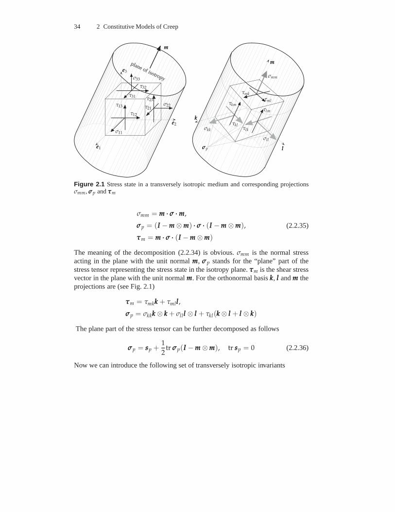
34 2 Constitutive Models of Creep
eee2
eee3
eee1
σ11
τ12
σ22
σ33
τ32
τ31
τ13 τ21
τ23
mmm
plane of isotropy
kkk
lll
mmm
σmm
τmk
τml
σkk
σll
τklτlk
τkmτlm
σσσp
Figure 2.1 Stress state in a transversely isotropic medium and corresponding projectionsσmm, σσσp andτττm
σmm = mmm ··· σσσ ···mmm,
σσσp = (III −mmm ⊗mmm) ··· σσσ ··· (III −mmm ⊗mmm),
τττm = mmm ··· σσσ ··· (III −mmm ⊗mmm)
(2.2.35)
The meaning of the decomposition (2.2.34) is obvious.σmm is the normal stressacting in the plane with the unit normalmmm, σσσp stands for the “plane” part of thestress tensor representing the stress state in the isotropyplane.τττm is the shear stressvector in the plane with the unit normalmmm. For the orthonormal basiskkk, lll andmmm theprojections are (see Fig. 2.1)
τττm = τmkkkk + τmllll,
σσσp = σkkkkk ⊗ kkk + σlllll ⊗ lll + τkl(kkk ⊗ lll + lll ⊗ kkk)
The plane part of the stress tensor can be further decomposedas follows
σσσp = sssp +1
2tr σσσp(III −mmm ⊗mmm), tr sssp = 0 (2.2.36)
Now we can introduce the following set of transversely isotropic invariants
2.2 Secondary Creep 35
I1m = σmm = mmm ··· σσσ ···mmm,
I2m = tr σσσp = tr σσσ −mmm ··· σσσ ···mmm,
I3m =1
2tr sss2
p =1
2tr σσσ2
p −1
4(tr σσσp)
2
=1
2
(
tr σσσ2 + (mmm ··· σσσ ···mmm)2)
−mmm ··· σσσ2 ···mmm − 1
4(tr σσσ −mmm ··· σσσ ···mmm)2,
I4m = τττm ··· τττm = mmm ··· σσσ2 ···mmm − (mmm ··· σσσ ···mmm)2 = (mmm × σσσ ···mmm) ··· (mmm × σσσ ···mmm)(2.2.37)
In the above listI2m and I3m are two invariants ofσσσp and I4m = τττ2m = τττm ··· τττm
is the square of the length of the shear stress vector acting in the plane with theunit normalmmm. It is shown in Sect. A.3.2 that the above invariants are integrals of(2.2.31).
Taking into account the relations
∂I1m
∂σσσ= mmm ⊗mmm,
∂I2m
∂σσσ= III −mmm ⊗mmm,
∂I3m
∂σσσ= sssp,
∂I4m
∂σσσ= τττmmm ⊗mmm + mmm ⊗ τττmmm
and the flow rule (2.1.6) we obtain the following creep equation
εεεcr =∂W
∂I1mmmm ⊗mmm +
∂W
∂I2m(III −mmm ⊗mmm) +
∂W
∂I3msssp
+∂W
∂I4m(τττmmm ⊗mmm + mmm ⊗ τττmmm)
(2.2.38)
The next assumption of the classical theory is the zero volumetric creep rate. Takingthe trace of (2.2.38) we obtain
tr εεεcr =∂W
∂I1m+ 2
∂W
∂I2m= 0 ⇒ W = W(I1m − 1
2I2m, I3m, I4m) (2.2.39)
Introducing the notation
Jm ≡ I1m − 1
2I2m = mmm ··· σσσ ···mmm − 1
2tr σσσp
the creep equation (2.2.38) takes the form
εεεcr =1
2
∂W
∂Jm(3mmm ⊗mmm − III) +
∂W
∂I3msssp +
∂W
∂I4m(τττmmm ⊗mmm + mmm ⊗ τττmmm) (2.2.40)
By analogy to the isotropic case we formulate the equivalentstress as follows
σ2eq = α1 J2
m + 3α2 I3m + 3α3 I4m
= α1
(
mmm ··· σσσ ···mmm − 1
2tr σσσp
)2
+3
2α2tr sss2
p + 3α3τ2mmm
(2.2.41)
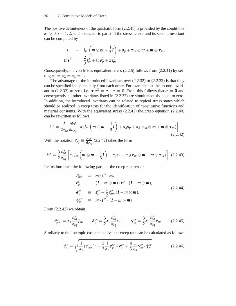
36 2 Constitutive Models of Creep
The positive definiteness of the quadratic form (2.2.41) is provided by the conditionsαi > 0, i = 1, 2, 3. The deviatoric partsss of the stress tensor and its second invariantcan be computed by
sss = Jm
(
mmm ⊗mmm − 1
3III
)
+ sssp + τττm ⊗mmm + mmm ⊗ τττm,
tr sss2 =2
3J2m + tr sss2
p + 2τ2mmm
Consequently, the von Mises equivalent stress (2.2.5) follows from (2.2.41) by set-ting α1 = α2 = α3 = 1.
The advantage of the introduced invariants over (2.2.32) or(2.2.33) is that theycan be specified independently from each other. For example,set the second invari-ant in (2.2.32) to zero, i.e.tr σσσ2 = σσσ ······ σσσ = 0. From this follows thatσσσ = 000 andconsequently all other invariants listed in (2.2.32) are simultaneously equal to zero.In addition, the introduced invariants can be related to typical stress states whichshould be realized in creep tests for the identification of constitutive functions andmaterial constants. With the equivalent stress (2.2.41) the creep equation (2.2.40)can be rewritten as follows
εεεcr =3
2σeq
∂W
∂σeq
[
α1 Jm
(
mmm ⊗mmm − 1
3III
)
+ α2sssp + α3(τττm ⊗mmm + mmm ⊗ τττm)
]
(2.2.42)
With the notationεcreq ≡ ∂W
∂σeq(2.2.42) takes the form
εεεcr =3
2
εcreq
σeq
[
α1 Jm
(
mmm ⊗mmm − 1
3III
)
+ α2sssp + α3(τττm ⊗mmm + mmm ⊗ τττm)
]
(2.2.43)
Let us introduce the following parts of the creep rate tensor
εcrmm ≡ mmm ··· εεεcr ···mmm,
εεεcrp ≡ (III −mmm ⊗mmm) ··· εεεcr ··· (III −mmm ⊗mmm),
ǫǫǫcrp ≡ εεεcr
p − 1
2εcr
mm(III −mmm ⊗mmm),
γγγcrm ≡ mmm ··· εεεcr ··· (III −mmm ⊗mmm)
(2.2.44)
From (2.2.42) we obtain
εcrmm = α1
εcreq
σeqJm, ǫǫǫcr
p =3
2α2
εcreq
σeqsssp, γγγcr
m =3
2α3
εcreq
σeqτττm (2.2.45)
Similarly to the isotropic case the equivalent creep rate can be calculated as follows
εcreq =
√
1
α1(εcr
mm)2 +2
3
1
α2ǫǫǫcr
p ······ ǫǫǫcrp +
4
3
1
α3γγγcr
m ··· γγγcrm (2.2.46)
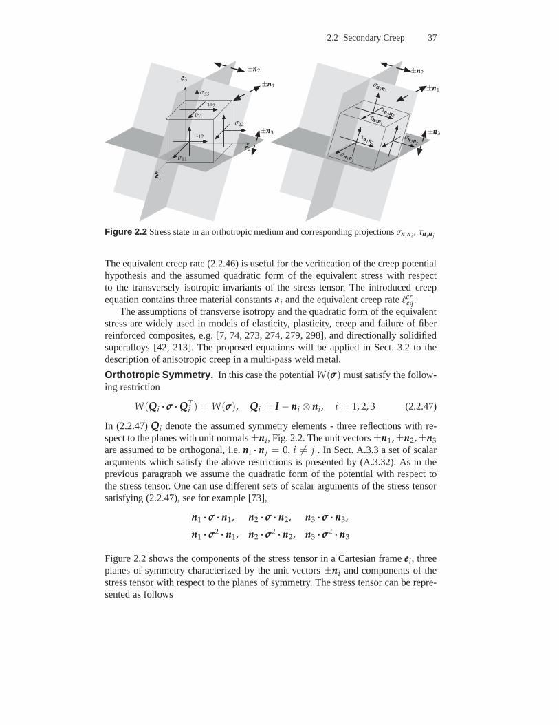
2.2 Secondary Creep 37
eee2
eee3
eee1
σ11
τ12
σ22
σ33
τ32
τ31
±nnn1±nnn1
±nnn2±nnn2
±nnn3±nnn3
σnnn1nnn1
τnnn1nnn2σnnn2nnn2
σnnn3nnn3
τnnn3nnn2τnnn3nnn1
Figure 2.2 Stress state in an orthotropic medium and corresponding projectionsσnnninnni, τnnninnnj
The equivalent creep rate (2.2.46) is useful for the verification of the creep potentialhypothesis and the assumed quadratic form of the equivalentstress with respectto the transversely isotropic invariants of the stress tensor. The introduced creepequation contains three material constantsαi and the equivalent creep rateεcr
eq.The assumptions of transverse isotropy and the quadratic form of the equivalent
stress are widely used in models of elasticity, plasticity,creep and failure of fiberreinforced composites, e.g. [7, 74, 273, 274, 279, 298], anddirectionally solidifiedsuperalloys [42, 213]. The proposed equations will be applied in Sect. 3.2 to thedescription of anisotropic creep in a multi-pass weld metal.
Orthotropic Symmetry. In this case the potentialW(σσσ) must satisfy the follow-ing restriction
W(QQQi ··· σσσ ··· QQQTi ) = W(σσσ), QQQi = III − nnni ⊗ nnni, i = 1, 2, 3 (2.2.47)
In (2.2.47)QQQi denote the assumed symmetry elements - three reflections with re-spect to the planes with unit normals±nnni, Fig. 2.2. The unit vectors±nnn1,±nnn2,±nnn3
are assumed to be orthogonal, i.e.nnni ··· nnnj = 0, i 6= j . In Sect. A.3.3 a set of scalararguments which satisfy the above restrictions is presented by (A.3.32). As in theprevious paragraph we assume the quadratic form of the potential with respect tothe stress tensor. One can use different sets of scalar arguments of the stress tensorsatisfying (2.2.47), see for example [73],
nnn1 ··· σσσ ··· nnn1, nnn2 ··· σσσ ··· nnn2, nnn3 ··· σσσ ··· nnn3,
nnn1 ··· σσσ2 ··· nnn1, nnn2 ··· σσσ2 ··· nnn2, nnn3 ··· σσσ2 ··· nnn3
Figure 2.2 shows the components of the stress tensor in a Cartesian frameeeei, threeplanes of symmetry characterized by the unit vectors±nnni and components of thestress tensor with respect to the planes of symmetry. The stress tensor can be repre-sented as follows
38 2 Constitutive Models of Creep
σσσ = σnnn1nnn1nnn1 ⊗ nnn1 + σnnn2nnn2nnn2 ⊗ nnn2 + σnnn3nnn3nnn3 ⊗ nnn3
+ τnnn1nnn2(nnn1 ⊗ nnn2 + nnn2 ⊗ nnn1) + τnnn1nnn3
(nnn1 ⊗ nnn3 + nnn3 ⊗ nnn1)
+ τnnn2nnn3(nnn2 ⊗ nnn3 + nnn3 ⊗ nnn2)
with
σnnn1nnn1= nnn1 ··· σσσ ··· nnn1, σnnn2nnn2 = nnn2 ··· σσσ ··· nnn2, σnnn3nnn3 = nnn3 ··· σσσ ··· nnn3,
τnnn1nnn2 = nnn1 ··· σσσ ··· nnn2, τnnn1nnn3 = nnn1 ··· σσσ ··· nnn3, τnnn2nnn3 = nnn2 ··· σσσ ··· nnn3
According to Sect. A.3.3 we use the following orthotropic invariants of the stresstensor
Innn1nnn1= σnnn1nnn1
, Innn2nnn2 = σnnn2nnn2 , Innn3nnn3 = σnnn3nnn3 ,
Innn1nnn2 = τ2nnn1nnn2
, Innn1nnn3 = τ2nnn1nnn3
, Innn2nnn3 = τ2nnn2nnn3
(2.2.48)
Assuming that the creep potential is a function of six arguments introduced, the flowrule (2.1.6) leads to the following creep equation
εεεcr =∂W
∂Innn1nnn1
nnn1 ⊗ nnn1 +∂W
∂Innn2nnn2
nnn2 ⊗ nnn2 +∂W
∂Innn3nnn3
nnn3 ⊗ nnn3
+∂W
∂Innn1nnn2
nnn1 ··· σσσ ··· nnn2(nnn1 ⊗ nnn2 + nnn2 ⊗ nnn1)
+∂W
∂Innn1nnn3
nnn1 ··· σσσ ··· nnn3(nnn1 ⊗ nnn3 + nnn3 ⊗ nnn1)
+∂W
∂Innn2nnn3
nnn2 ··· σσσ ··· nnn3(nnn2 ⊗ nnn3 + nnn3 ⊗ nnn2)
(2.2.49)
The assumption of zero volumetric creep rate leads to
tr εεεcr =∂W
∂Innn1nnn1
+∂W
∂Innn2nnn2
+∂W
∂Innn3nnn3
= 0 (2.2.50)
From the partial differential equation (2.2.50) follows that the potentialW is afunction of five scalar arguments of the stress tensor. The characteristic system of(2.2.50) is
dInnn1nnn1
ds= 1,
dInnn2nnn2
ds= 1,
dInnn3nnn3
ds= 1 (2.2.51)
The above system of three ordinary differential equations has two independent inte-grals. One can verify that the following invariants
J1 =1
2(Innn2nnn2 − Innn3nnn3), J2 =
1
2(Innn3nnn3 − Innn1nnn1
), J3 =1
2(Innn1nnn1
− Innn2nnn2)
(2.2.52)are integrals of (2.2.51). Only two of them are independent due to the relationJ1 + J2 + J3 = 0. If the principal directions of the stress tensor coincide with thedirectionsnnni thenτnnninnnj
= 0, i 6= j and the above invariants represent the principalshear stresses. An alternative set of integrals of (2.2.51)is
2.2 Secondary Creep 39
J1 = Innn1nnn1 −1
3tr σσσ, J2 = Innn2nnn2 −
1
3tr σσσ, J3 = Innn3nnn3 −
1
3tr σσσ (2.2.53)
If the principal directions of the stress tensor coincide with nnni then the above invari-ants are the principal values of the stress deviator. For theformulation of the creeppotential in terms of invariants the relationJ1 + J2 + J3 = 0 must be taken intoaccount.
In what follows we apply the invariants (2.2.52). The equivalent stress can beformulated as follows
σ2eq = 2β1 J2
1 + 2β2 J22 + 2β3 J2
3
+ 3β12 Innn1nnn2 + 3β13 Innn1nnn3 + 3β23 Innn2nnn3
(2.2.54)
The von Mises equivalent stress (2.2.5) follows from (2.2.54) by settingβ1 = β2 =β3 = β12 = β13 = β23 = 1. Applying the flow rule (2.1.6) we obtain the followingcreep equation
εεεcr =εcr
eq
σeq
[
β1 J1(nnn2 ⊗ nnn2 − nnn3 ⊗ nnn3)
+β2 J2(nnn3 ⊗ nnn3 − nnn1 ⊗ nnn1)
+β3 J3(nnn1 ⊗ nnn1 − nnn2 ⊗ nnn2)
+3
2β12τnnn1nnn2(nnn1 ⊗ nnn2 + nnn2 ⊗ nnn1)
+3
2β13τnnn1nnn3(nnn1 ⊗ nnn3 + nnn3 ⊗ nnn1)
+3
2β23τnnn2nnn3(nnn2 ⊗ nnn3 + nnn3 ⊗ nnn2)
]
(2.2.55)
The equivalent stress and the creep equation includes six independent materialconstants. Therefore six independent homogeneous stress states should be realizedin order to identify the whole set of constants. In addition,the dependence of thecreep rate on the equivalent stress must be fitted from the results of uni-axial creeptests for different constant stress values. For example, ifthe power law stress func-tion provides a satisfactory description of steady-state creep then the constantnmust be additionally identified.
An example of orthotropic creep is discussed in [163] for thealuminium alloyD16AT. Plane specimens were removed from rolled sheet alongthree directions:the rolling direction, the transverse direction as well as under the angle of 45 to therolling direction. Uni-axial creep tests were performed at273C and 300C withinthe stress range 63-90 MPa. The results have shown that at 273C creep curvesdepend on the loading direction while at 300C the creep behavior is isotropic.
Other cases. The previous models are based on the assumption of the quadraticform of the creep potential with respect to the stress tensor. The most generalquadratic form can be formulated as follows
σ2eq =
1
2σσσ ······ (4)BBB ······ σσσ, (2.2.56)
40 2 Constitutive Models of Creep
whereσeq plays the role of the equivalent stress. The fourth rank tensor (4)BBB mustsatisfy the following restrictions
aaa ······ (4)BBB ······ aaa ≥ 0, aaa ······ (4)BBB = (4)BBB ······ aaa, ccc ······ (4)BBB = 000,
∀ aaa, ccc with aaa = aaaT, ccc = −cccT,(2.2.57)
whereaaa andccc are second rank tensors. Additional restrictions follow from the as-sumed symmetries of the steady state creep behavior. For example, if the orthogonaltensorQQQ stands for a symmetry element, the structure of the tensor(4)BBB can be es-tablished from the following equation
(4)BBB′ = BijklQQQ ··· eeei ⊗QQQ ··· eeej ⊗QQQ ··· eeek ⊗QQQ ··· eeel =(4)BBB, (2.2.58)
whereeeei, i = 1, 2, 3 are basis vectors.The flow rule (2.1.6) provides the following generalized anisotropic creep equa-
tion
εεεcr =εcr
eq
2σeq
(4)BBB ······ σσσ, εcreq ≡ ∂W
∂σeq(2.2.59)
The fourth rank tensors satisfying the restrictions (2.2.57) are well-known fromthe theory of linear elasticity. They are used to represent elastic material proper-ties in the generalized Hooke’s law. The components of thesetensors in a Carte-sian coordinate system are given in the matrix notation in many textbooks on lin-ear elasticity as well as in books and monographs on composite materials, e.g.[6, 7, 29, 122, 256, 309]. Furthermore, different coordinate free representations offourth rank tensors of this type are discussed in the literature. For a review we re-fer to [76]. One of these representations - the projector representation is applied in[47, 48, 200] to constitutive modeling of creep in single crystal alloys under as-sumption of the cubic symmetry.
Let us recall that (2.2.59) is the consequence of the creep potential hypothesisand the quadratic form of the equivalent stress with respectto the stress tensor.Similarly to the case of linear elasticity [309] one can prove that only eight basicsymmetry classes are relevant according to these assumptions. The basic symmetryclasses and the corresponding number of independent coordinates of the tensor(4)BBBare listed in Table 2.1. The number of independent coordinates indicates the numberof material constants which should be identified from creep tests. This number canbe reduced if the volume constancy is additionally assumed.For example, in thecases of transverse isotropy and orthotropic symmetry the number of independentcoordinates ofBBB reduces to 3 and 5, respectively (see previous paragraphs).
2.2.2.2 Non-classical Creep Equations. Non-classical effects are the depen-dence of secondary creep rate on the kind of loading and second order effects,see Sect. 2.2.1. Examples of such behavior are different creep rates under ten-sile and compressive stress or the effect of reversal of the shear stress. The lastcase is observed in creep tests on tubular specimens under applied torque. Thechange of the direction of the applied torque leads to different values of the shear
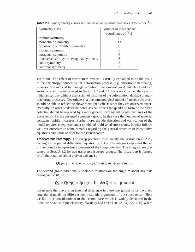
2.2 Secondary Creep 41
Table 2.1 Basic symmetry classes and number of independent coordinates of the tensor(4)BBB
Symmetry class Number of independentcoordinates of(4)BBB
triclinic symmetry 21monoclinic symmetry 13orthotropic or rhombic symmetry 9trigonal symmetry 6tetragonal symmetry 6transverse isotropy or hexagonal symmetry 5cubic symmetry 3isotropic symmetry 2
strain rate. The effect of shear stress reversal is usually explained to be the resultof the anisotropy induced by the deformation process (e.g. anisotropic hardening)or anisotropy induced by damage evolution. Phenomenological models of inducedanisotropy will be introduced in Sect. 2.3.2 and 2.4. Here weconsider the case ofinitial anisotropy without discussion of histories of the deformation, damage or man-ufacturing processes. Nevertheless, a phenomenological model of anisotropic creepshould be able to reflect the above mentioned effects since they are observed exper-imentally. In order to describe non-classical effects the quadratic form of the creeppotential should be replaced by a more general form including all invariants of thestress tensor for the assumed symmetry group. In this case the number of materialconstants rapidly increases. Furthermore, the identification and verification of themodel requires creep tests under combined multi-axial stress states. In what followswe limit ourselves to some remarks regarding the general structure of constitutiveequations and kinds of tests for the identification.
Transverse isotropy. The creep potential must satisfy the restriction (2.2.29)leading to the partial differential equation (2.2.30). Theintegrals represent the setof functionally independent arguments of the creep potential. The integrals are pre-sented in Sect. A.3.2 for two transverse isotropy groups. The first group is formedby all the rotations about a given axismmm, i.e
QQQ(ψmmm) = mmm ⊗mmm + cos ψ(III −mmm ⊗mmm) + sin ψmmm × III
The second group additionally includes rotations on the angle π about any axisorthogonal tommm, i.e.
QQQ1 = QQQ(πppp) = 2ppp ⊗ ppp − III, det QQQ = 1, ppp ···mmm = 0
Let us note that there is an essential difference in these twogroups since the creeppotential depends on different non-quadratic arguments ofthe stress tensor. Herewe limit our considerations to the second case which is widely discussed in theliterature on anisotropic elasticity, plasticity and creep [58, 73, 84, 279, 286], where
42 2 Constitutive Models of Creep
the following invariants are applied2
tr σσσ, tr σσσ2, tr σσσ3, mmm ··· σσσ ···mmm, mmm ··· σσσ2 ···mmm (2.2.60)
To be consistent with derivations in Sect. 2.2.2.1 let us usethe decomposition of thestress tensor (2.2.34) leading to the following set of invariants
I1m = σmm = mmm ··· σσσ ···mmm,
I2m = tr σσσp = tr σσσ −mmm ··· σσσ ···mmm,
I3m =1
2tr sss2
p =1
2tr σσσ2
p −1
4(tr σσσp)
2
=1
2
[
tr σσσ2 + (mmm ··· σσσ ···mmm)2]
−mmm ··· σσσ2 ···mmm − 1
4(tr σσσ −mmm ··· σσσ ···mmm)2,
I4m = τττm ··· τττm = mmm ··· σσσ2 ···mmm − (mmm ··· σσσ ···mmm)2 = (mmm × σσσ ···mmm) ··· (mmm × σσσ ···mmm)
I5m = τττm ··· sssp ··· τττm = mmm ··· σσσ3 ···mmm − 2(mmm ··· σσσ ···mmm)(mmm ··· σσσ2 ···mmm)
+ (mmm ··· σσσ ···mmm)3 − 1
2(tr σσσ −mmm ··· σσσ ···mmm)
[
mmm ··· σσσ2 ···mmm − (mmm ··· σσσ ···mmm)2]
(2.2.61)The meaning of the first four invariants is explained in in Sect. 2.2.2.1. The lastcubic invariant is introduced insteadtr σσσ3. One can prove the following relation
tr σσσ3 = I31m + 3I1m I4m + 3I2m I3m +
3
2I2m I4m +
1
2I32m + 3I5m
Assuming that the creep potentialW is a function of five scalar arguments (2.2.61)and applying the flow rule (2.1.6) we obtain the following creep equation
εεεcr = h1mmm ⊗mmm + (h2−1
2h5 I4m)(III −mmm ⊗mmm) + h3σσσp + h4(τττm ⊗mmm + mmm ⊗ τττm)
+h5
(
τττm ⊗ τττm + mmm ⊗ σσσp ··· τττm + τττm ··· σσσp ⊗mmm)
,(2.2.62)
where
hi =∂W
∂Iim, i = 1, 2, . . . , 5
The last term in the right-hand side of (2.2.62) describes second order effects. Themeaning of these effects is obvious. In the case of non-zero “transverse shear stress”vector
τττm = mmm ··· σσσ ··· (III −mmm ⊗mmm)
the elongation in the direction ofτττm can be considered. The vectorςςςm = sssp ··· τττm
belongs to the isotropy plane, i.e.ςςςm ··· mmm = 0. In the case thatςςςm 6= 000 (2.2.62)describes an additional “transverse shear strain rate” effect.
2 For the description of elastic material behavior instead ofσσσ a strain tensor, e.g. the Cauchy-Green strain tensor is introduced. The five transversely isotropic invariants are the argu-ments of the strain energy density function.
2.2 Secondary Creep 43
In order to formulate the creep constitutive equation one should specify an ex-pression for the equivalent stress as a function of the introduced invariants. As anexample we present the equivalent stress by use of polynomials of the type (2.2.9)and (2.2.10)
σeq = ασ1 + σ2 + γσ3, (2.2.63)
with
σ1 = µ11 I1m + µ12 I2m,
σ2 = µ21 I21m + µ22 I1m I2m + µ23 I2
2m + µ24 I3m + µ25 I4m,
σ3 = µ31 I31m + µ32 I2
1m I2m + µ33 I1m I22m + µ34 I3
2m + µ35 I1m I3m
+ µ36 I2m I3m + µ37 I1m I4m + µ38 I2m I4m + µ39 I5m
(2.2.64)
The equivalent stress (2.2.63) includes 16 material constants µij and two weight-ing factorsα and γ. The identification of all material constants requires differ-ent independent creep tests under multi-axial stress states. For example, in orderto find the constantµ39 creep tests under stress states with nonzero cubic invari-ant I5m should be carried out. An example is the tension in the isotropy planecombined with the transverse shear stress leading to the stress state of the typeσσσ = σ0nnn1 ⊗ nnn1 + τ0(nnn1 ⊗mmm + mmm ⊗ nnn1), whereσ0 > 0 andτ0 > 0 are the mag-nitudes of the applied stresses,nnn1 is the direction of tension andnnn1 ···mmm = 0. In thiscase
sssp =1
2σ0(nnn1 ⊗ nnn1 − nnn2 ⊗ nnn2), nnn1 ··· nnn2 = 0, τττm = τ0nnn1, I5m =
1
2σ0τ2
0
By analogy to the non-classical models of isotropic creep discussed in Sect.2.2.1 different special cases can be introduced. Settingγ = 0 in (2.2.64), secondorder effects will be neglected. The resulting constitutive model takes into accountdifferent behavior under tension and compression. To find the constantsµ11 andµ12
creep tests under tension (compression) along the direction mmm as well as tension(compression) along any direction in the isotropy plane should be carried out. Set-ting α = 0 the model with the quadratic form of the creep potential with5 constantscan be obtained. The assumption of the zero volumetric creeprate will lead to themodel discussed in Sect. 2.2.2.1.
Second order effects of anisotropic creep were discussed byBetten [52, 58].He found disagreements between creep equations based on thetheory of isotropicfunctions and the creep equation of the type (2.2.62) according to the potential hy-pothesis and the flow rule. The conclusion was made that the potential theory leadsto restrictive forms of constitutive equations if comparedto the representations oftensor functions.
Let us recall the results following from the algebra of isotropic tensor functions[71]. In the case of transverse isotropy group characterized by the symmetry ele-ments (A.3.18) the statement of the problem is to find the general representation ofthe isotropic tensor function of the stress tensorσσσ and the dyadmmm ⊗ mmm (so-called
44 2 Constitutive Models of Creep
structure tensor). The constitutive equation describing the creep behavior must befound as follows
εεεcr = fff (σσσ, mmm ⊗mmm),
where fff is an isotropic tensor function of two tensor arguments. Thegeneral repre-sentation of this function is [73]
fff (σσσ, mmm ⊗mmm) = f1mmm ⊗mmm + f2(III −mmm ⊗mmm) + f3σσσ + f4σσσ2
+ f5(mmm ⊗mmm ··· σσσ + σσσ ···mmm ⊗mmm) + f6(mmm ⊗mmm ··· σσσ2+ σσσ2 ···mmm ⊗mmm),(2.2.65)
where the scalarsfi, i = 1, . . . , 6, depend on the five invariants of the stress tensor(2.2.60). Betten found that the last term in (2.2.65) is missing in the constitutiveequation which is based on the potential theory. In order to discuss the meaningof the last term in (2.2.65) let us introduce the identities which follow from thedecomposition of the stress tensor by Eqs (2.2.34) and (2.2.36)
σσσ2 = I2msssp + (I3m +1
4I22m)(III −mmm ⊗mmm) + mmm ⊗ sssp ··· τττm + τττm ··· sssp ⊗mmm
+ (I1m +1
2I2m)(τττm ⊗mmm + mmm ⊗ τττm) + (I2
1m + I4m)mmm ⊗mmm + τττm ⊗ τττm,
(2.2.66)mmm ⊗mmm ··· σσσ + σσσ ···mmm ⊗mmm = τττm ⊗mmm + mmm ⊗ τττm + 2I1mmmm ⊗mmm,
mmm ⊗mmm ··· σσσ2 + σσσ2 ···mmm ⊗mmm = mmm ⊗ sssp ··· τττm + τττm ··· sssp ⊗mmm
+ (I1m +1
2I2m)(τττm⊗mmm + mmm⊗τττm)
+ 2(I4m + I21m)mmm⊗mmm
After inserting (2.2.66), (2.2.34) and (2.2.36) into (2.2.65) we obtain the followingcreep equation
εεεcr = g1mmm ⊗mmm + g2(III −mmm ⊗mmm) + g3sssp + g4(mmm ⊗ τττm + τττm ⊗mmm)
+ g5(mmm ⊗ sssp ··· τττm + τττm ··· sssp ⊗mmm) + g6τττm ⊗ τττm
(2.2.67)with
g1 = f1 + f4(I21m + I4m) + 2 f5 I1m + 2 f6(I4m + I2
1m),
g2 = f2 +1
2f3 I2m + f 4(I3m +
1
4I22m),
g3 = f3 + I2m f4,
g4 = ( f4 + f6)(I1m +1
2I2m) + f5,
g5 = f4 + f6,
g6 = f4
2.2 Secondary Creep 45
We observe that Eq. (2.2.67) based on the theory of isotropictensor functions doesnot deliver any new second order effect in comparison to (2.2.62). The only dif-ference is that the two last terms in (2.2.67) characterizing the second order ef-fects appear with two different influence functions. The comparison of (2.2.67) with(2.2.62) provides the following conditions for the existence of the potential
∂W
∂I1m= g1,
∂W
∂I2m= g2 +
1
2g5 I4m,
∂W
∂I3m= g3,
∂W
∂I4m= g4,
∂W
∂I5m= g5, g6 = g5
Furthermore, the functionsgi must satisfy the integrability conditions which can beobtained by equating the mixed derivatives of the potentialwith respect to invariants,i.e.
∂2W
∂Iim∂Ikm=
∂2W
∂Ikm∂Iim, i 6= k, i, k = 1, 2, . . . , 5
Let us note that the models (2.2.62) and (2.2.67) are restricted to the special case oftransverse isotropy. In the general case one should analyzethe creep potential withthe invariants listed in (A.3.26).
Other cases. Alternatively a phenomenological constitutive equation of aniso-tropic creep can be formulated with the help of material tensors, e.g. [2]. Introduc-ing three material tensorsAAA, (4)BBB and (6)CCC the equivalent stress (2.2.63) can begeneralized as follows
σeq = ασ1 + σ2 + γσ3 (2.2.68)
with
σ1 = AAA ······ σσσ, σ22 = σσσ ······ (4)BBB ······ σσσ, σ3
3 = σσσ ······ (σσσ ······ (6)CCC ······ σσσ) (2.2.69)
The structure of the material tensors must be established from the following restric-tions
AAA′ = QQQ ··· AAA ···QQQT = AijQQQ ··· eeei ⊗QQQ ··· eeej = AAA,
(4)BBB′ = BijklQQQ ··· eeei ⊗QQQ ··· eeej ⊗QQQ ··· eeek ⊗QQQ ··· eeel =(4)BBB,
(6)CCC′ = CijklmnQQQ ··· eeei ⊗QQQ ··· eeej ⊗QQQ ··· eeek ⊗QQQ ··· eeel ⊗QQQ ··· eeem ⊗QQQ ··· eeen =(6)CCC,(2.2.70)
whereQQQ is an element of the physical symmetry group. The creep potential hypoth-esis and the flow rule (2.1.6) lead to the following creep equation
εεεcr =∂W
∂σeq
(
α∂σ1
∂σσσ+
∂σ2
∂σσσ+ γ
∂σ3
∂σσσ
)
(2.2.71)
Taking into account the relations
∂σ1
∂σσσ= AAA,
∂σ2
∂σσσ=
(4)BBB ······ σσσ
σ2,
∂σ3
∂σσσ=
σσσ ······ (6)CCC ······ σσσ
σ23
(2.2.72)
46 2 Constitutive Models of Creep
a generalized anisotropic creep equation can be formulatedas follows
εεεcr = εcreq
(
αAAA +(4)BBB ······ σσσ
σ2+ γ
σσσ ······ (6)CCC ······ σσσ
σ23
)
, εcreq ≡
∂W
∂σeq(2.2.73)
In [51, 265] the following anisotropic creep equation is proposed
εεεcr = HHH + (4)MMM ······ σσσ + ((6)LLL ······ σσσ) ······ σσσ (2.2.74)
Comparing the Eqs (2.2.73) and (2.2.74) the material tensors HHH, (4)MMM and(6)LLL canbe related to the tensorsAAA, (4)BBB and(6)CCC.
The tensorsAAA, (4)BBB and (6)CCC contain 819 coordinates (AAA - 9, (4)BBB - 81, (6)CCC- 729). From the symmetry of the stress tensor and the creep rate tensor as well asfrom the potential hypothesis follows that “only” 83 coordinates are independent (AAA- 6, (4)BBB - 21, (6)CCC - 56). Further reduction is based on the symmetry considerations.The structure of material tensors and the number of independent coordinates can beobtained by solving (2.2.70).
Another possibility of simplification is the establishing of special cases of(2.2.73). For instance, equations with a reduced number of parameters can be de-rived as follows
– α = 1, γ = 0:
σeq = σ1 + σ2, εεεcr = εcreq
(
AAA +(4)BBB ······ σσσ
σ2
)
, (2.2.75)
– α = 0, γ = 1:
σeq = σ2 + σ3, εεεcr = εcreq
(
(4)BBB ······ σσσ
σ2+
σσσ ······ (6)CCC ······ σσσ
σ23
)
, (2.2.76)
– α = 0, γ = 0:
σeq = σ2, εεεcr = εcreq
(
(4)BBB ······ σσσ
σ2
)
(2.2.77)
The last case has been discussed in Sect. 2.2.2.1. Examples of application of con-stitutive equation (2.2.73) as well as different cases of symmetries are discussed in[2, 9].
2.2.3 Functions of Stress and Temperature
In all constitutive equations discussed in Sects 2.2.1 and 2.2.2 the creep potential orthe equivalent creep rate must be specified as functions of the equivalent stress andthe temperature, i.e.
εcreq =
∂W
∂σeq= f (σeq, T)
2.2 Secondary Creep 47
In [176] the functionf is termed to be the constitutive or response function. For theformulation of constitutive functions one may apply theoretical foundations frommaterials science with regard to mechanisms of creep deformation and related formsof stress and temperature functions. Furthermore, experimental data including fam-ilies of creep curves obtained from uni-axial creep tests for certain ranges of stressand temperature are required. It is convenient to present these families in a formof minimum creep rate vs. stress and minimum creep rate vs. temperature curvesin order to find mechanical properties of the material withinthe steady-state creeprange.
Many empirical functions of stress and temperature which allow to fit exper-imental data have been proposed in the literature, e.g. [236, 250, 266, 292]. Thestarting point is the assumption that the creep rate may be descried as a product oftwo separate functions of stress and temperature
εcreq = fσ(σeq) fT(T)
The widely used functions of stress are:
– power law
fσ(σeq) = ε0
∣
∣
∣
∣
σeq
σ0
∣
∣
∣
∣
n−1 σeq
σ0(2.2.78)
The power law contains three constants (ε0, σ0, n) but only two of them are inde-pendent. Instead ofε0 andσ0 one material constant
a ≡ ε0
σn0
can be introduced.– power law including the creep limit
fσ(σeq) = ε′0
(
σeq
σ′0
− 1
)n′
, σeq > σ′0
If σeq ≤ σ′0 the creep rate is equal zero. In this caseσ′
0 is the assumed creep limit.Let us note that the experimental identification of its valueis difficult, e.g. [266].
– exponential law
fσ(σeq) = ε0 expσeq
σ0
ε0, σ0 are material constants. The disadvantage of this expression is that it predictsa nonzero creep rate for a zero equivalent stress
fσ(0) = ε0 6= 0
– hyperbolic sine law
fσ(σeq) = ε0 sinhσeq
σ0
48 2 Constitutive Models of Creep
For low stress values this function provides the linear dependence on the stress
fσ(σeq) ≈ ε0σeq
σ0
Assuming the constant temperature equations for the equivalent creep rate can besummarized as follows
εcreq = aσn
eq Norton, 1929, Bailey, 1929,
εcreq = b
(
expσeq
σ0− 1
)
Soderberg, 1936,
εcreq = a sinh
σeq
σ0Prandtl, 1928, Nadai, 1938, McVetty, 1943,
εcreq = a1σ
n1eq + a2σn2
eq Johnson et al., 1963,
εcreq = a
(
sinhσeq
σ0
)n
Garofalo, 1965,
(2.2.79)
wherea, b, a1, a2, σ0, n, n1 and n2 are material constants. The dependence on thetemperature is usually expressed by the Arrhenius law
fT(T) = exp[−Q/RT],
whereQ andR denote the activation energy and the Boltzmann’s constant,respec-tively.
For the use of stress and temperature functions one should take into accountthat different deformation mechanisms may operate for different specific ranges ofstress and temperature. An overview is provided by the deformation mechanismsmaps proposed by Frost and Ashby [117], Fig. 2.3. Contours ofconstant strain ratesare presented as functions of the normalized equivalent stressσeq/G and the ho-mologous temperatureT/Tm, whereG is the shear modulus andTm is the meltingtemperature. For a given combination of the stress and the temperature, the mapprovides the dominant creep mechanism and the strain rate.
Let us briefly discuss different regions on the map, the mechanisms of creepdeformation and constitutive functions derived in materials science. For compre-hensive reviews one may consult [116, 156, 222]. The originsof the inelastic de-formation at the temperature range0.5 < T/Tm < 0.7 are transport processesassociated with motion and interaction of dislocations anddiffusion of vacancies.Here we limit our consideration to the two classes of physical models - dislocationand diffusion creep. Various creep rate equations within the dislocation creep rangeare based on the Bailey-Orowan recovery hypothesis. An internal barrier stressσint
being opposed to the dislocation movement is assumed. When the plastic strain oc-curs the internal stress increases as a result of work hardening due to accumulationof deformation and due to increase of the dislocation density. As the material is sub-jected to the load and temperature over certain time, the internal stressσint recovers.In the uni-axial case the rate of change of the internal stress is assumed as follows
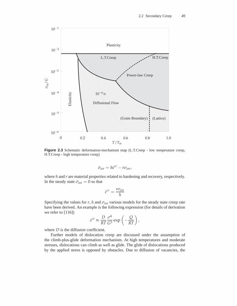
2.2 Secondary Creep 49
0 0.2 0.4 0.6 0.8 1.0
10−6
10−5
10−4
10−3
10−2
10−1
Plasticity
Diffusional Flow
(Grain Boundary) (Lattice)
Ela
stic
ity
Power-law Creep
T/Tm
σeq
/G
10−6/s
L.T.Creep H.T.Creep
Figure 2.3 Schematic deformation-mechanism map (L.T.Creep - low temperature creep,H.T.Creep - high temperature creep)
σint = hεcr − rσint,
whereh andr are material properties related to hardening and recovery,respectively.In the steady stateσint = 0 so that
εcr =rσint
h
Specifying the values forr, h andσint various models for the steady state creep ratehave been derived. An example is the following expression (for details of derivationwe refer to [116])
εcr ∝D
RT
σ4
G3exp
(
− Q
RT
)
,
whereD is the diffusion coefficient.Further models of dislocation creep are discussed under theassumption of
the climb-plus-glide deformation mechanism. At high temperatures and moderatestresses, dislocations can climb as well as glide. The glideof dislocations producedby the applied stress is opposed by obstacles. Due to diffusion of vacancies, the
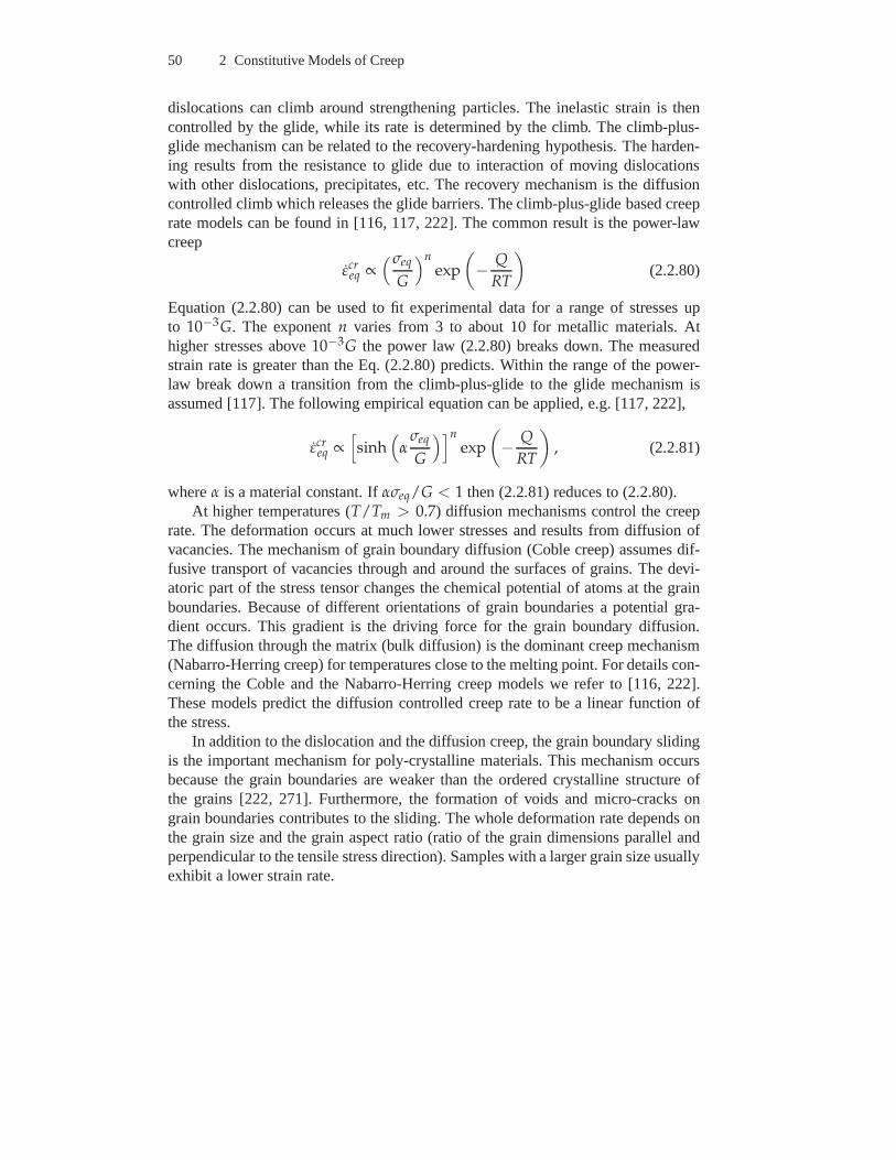
50 2 Constitutive Models of Creep
dislocations can climb around strengthening particles. The inelastic strain is thencontrolled by the glide, while its rate is determined by the climb. The climb-plus-glide mechanism can be related to the recovery-hardening hypothesis. The harden-ing results from the resistance to glide due to interaction of moving dislocationswith other dislocations, precipitates, etc. The recovery mechanism is the diffusioncontrolled climb which releases the glide barriers. The climb-plus-glide based creeprate models can be found in [116, 117, 222]. The common resultis the power-lawcreep
εcreq ∝
(σeq
G
)nexp
(
− Q
RT
)
(2.2.80)
Equation (2.2.80) can be used to fit experimental data for a range of stresses upto 10−3G. The exponentn varies from 3 to about 10 for metallic materials. Athigher stresses above10−3G the power law (2.2.80) breaks down. The measuredstrain rate is greater than the Eq. (2.2.80) predicts. Within the range of the power-law break down a transition from the climb-plus-glide to theglide mechanism isassumed [117]. The following empirical equation can be applied, e.g. [117, 222],
εcreq ∝
[
sinh(
ασeq
G
)]nexp
(
− Q
RT
)
, (2.2.81)
whereα is a material constant. Ifασeq/G < 1 then (2.2.81) reduces to (2.2.80).At higher temperatures (T/Tm > 0.7) diffusion mechanisms control the creep
rate. The deformation occurs at much lower stresses and results from diffusion ofvacancies. The mechanism of grain boundary diffusion (Coble creep) assumes dif-fusive transport of vacancies through and around the surfaces of grains. The devi-atoric part of the stress tensor changes the chemical potential of atoms at the grainboundaries. Because of different orientations of grain boundaries a potential gra-dient occurs. This gradient is the driving force for the grain boundary diffusion.The diffusion through the matrix (bulk diffusion) is the dominant creep mechanism(Nabarro-Herring creep) for temperatures close to the melting point. For details con-cerning the Coble and the Nabarro-Herring creep models we refer to [116, 222].These models predict the diffusion controlled creep rate tobe a linear function ofthe stress.
In addition to the dislocation and the diffusion creep, the grain boundary slidingis the important mechanism for poly-crystalline materials. This mechanism occursbecause the grain boundaries are weaker than the ordered crystalline structure ofthe grains [222, 271]. Furthermore, the formation of voids and micro-cracks ongrain boundaries contributes to the sliding. The whole deformation rate depends onthe grain size and the grain aspect ratio (ratio of the grain dimensions parallel andperpendicular to the tensile stress direction). Samples with a larger grain size usuallyexhibit a lower strain rate.
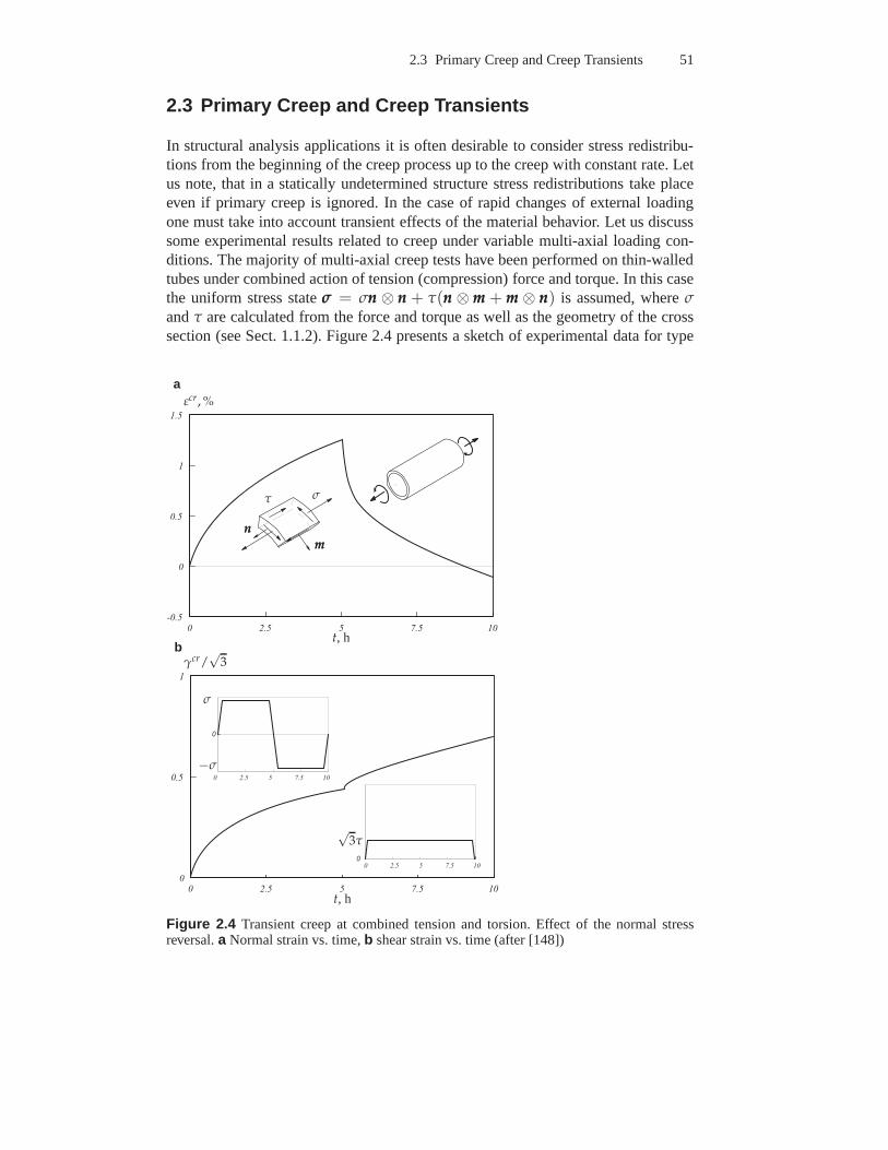
2.3 Primary Creep and Creep Transients 51
2.3 Primary Creep and Creep Transients
In structural analysis applications it is often desirable to consider stress redistribu-tions from the beginning of the creep process up to the creep with constant rate. Letus note, that in a statically undetermined structure stressredistributions take placeeven if primary creep is ignored. In the case of rapid changesof external loadingone must take into account transient effects of the materialbehavior. Let us discusssome experimental results related to creep under variable multi-axial loading con-ditions. The majority of multi-axial creep tests have been performed on thin-walledtubes under combined action of tension (compression) forceand torque. In this casethe uniform stress stateσσσ = σnnn ⊗ nnn + τ(nnn ⊗ mmm + mmm ⊗ nnn) is assumed, whereσandτ are calculated from the force and torque as well as the geometry of the crosssection (see Sect. 1.1.2). Figure 2.4 presents a sketch of experimental data for type
0 2 . 5 5 7 . 5 1 0- 0 . 5
0
0 . 5
1
1 . 5
0 2 . 5 5 7 . 5 1 00
0 . 5
1
0 2 . 5 5 7 . 5 1 0
0
0 2 . 5 5 7 . 5 1 00
t, h
t, h
εcr, %
γcr/√
3
σ
σ
−σ
√3τ
τ
nnnmmm
a
b
Figure 2.4 Transient creep at combined tension and torsion. Effect of the normal stressreversal.a Normal strain vs. time,b shear strain vs. time (after [148])
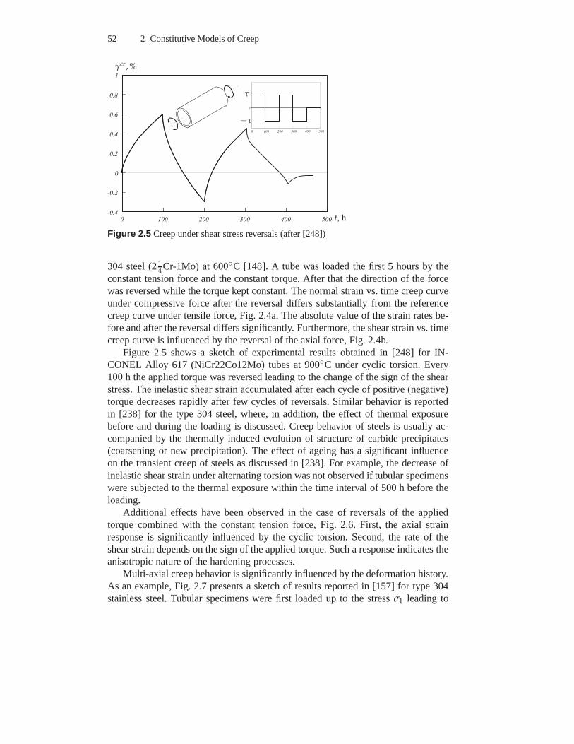
52 2 Constitutive Models of Creep
0 1 0 0 2 0 0 3 0 0 4 0 0 5 0 0- 0 . 4
- 0 . 2
0
0 . 2
0 . 4
0 . 6
0 . 8
1
0 1 0 0 2 0 0 3 0 0 4 0 0 5 0 0
0
t, h
γcr, %
τ
−τ
Figure 2.5 Creep under shear stress reversals (after [248])
304 steel (214Cr-1Mo) at 600C [148]. A tube was loaded the first 5 hours by theconstant tension force and the constant torque. After that the direction of the forcewas reversed while the torque kept constant. The normal strain vs. time creep curveunder compressive force after the reversal differs substantially from the referencecreep curve under tensile force, Fig. 2.4a. The absolute value of the strain rates be-fore and after the reversal differs significantly. Furthermore, the shear strain vs. timecreep curve is influenced by the reversal of the axial force, Fig. 2.4b.
Figure 2.5 shows a sketch of experimental results obtained in [248] for IN-CONEL Alloy 617 (NiCr22Co12Mo) tubes at 900C under cyclic torsion. Every100 h the applied torque was reversed leading to the change ofthe sign of the shearstress. The inelastic shear strain accumulated after each cycle of positive (negative)torque decreases rapidly after few cycles of reversals. Similar behavior is reportedin [238] for the type 304 steel, where, in addition, the effect of thermal exposurebefore and during the loading is discussed. Creep behavior of steels is usually ac-companied by the thermally induced evolution of structure of carbide precipitates(coarsening or new precipitation). The effect of ageing hasa significant influenceon the transient creep of steels as discussed in [238]. For example, the decrease ofinelastic shear strain under alternating torsion was not observed if tubular specimenswere subjected to the thermal exposure within the time interval of 500 h before theloading.
Additional effects have been observed in the case of reversals of the appliedtorque combined with the constant tension force, Fig. 2.6. First, the axial strainresponse is significantly influenced by the cyclic torsion. Second, the rate of theshear strain depends on the sign of the applied torque. Such aresponse indicates theanisotropic nature of the hardening processes.
Multi-axial creep behavior is significantly influenced by the deformation history.As an example, Fig. 2.7 presents a sketch of results reportedin [157] for type 304stainless steel. Tubular specimens were first loaded up to the stressσ1 leading to
2.3 Primary Creep and Creep Transients 53
0 5 0 1 0 0 1 5 0 2 0 0 2 5 0 3 0 0 3 5 0 4 0 0 4 5 0- 2
- 1 . 5
- 1
- 0 . 5
0
0 . 5
1
0 5 0 1 0 0 1 5 0 2 0 0 2 5 0 3 0 0 3 5 0 4 0 0 4 5 00
0 . 5
1
1 . 5
2
2 . 5
3
0 1 0 0 2 0 0 3 0 0 4 0 0 5 0 0
0 1 0 0 2 0 0 3 0 0 4 0 0 5 0 0
0
t, h
t, h
εcr, %
γcr, %
τ
−τ
σ
a
b
Figure 2.6 Creep at combined tension and torsion. Effect of the shear stress reversals.aNormal strain vs. time,b shear strain vs. time (after [248])
the plastic strain of3%. After that the specimens were unloaded toσ0. Subsequentcreep tests have been performed under combined constant normal strainσ and shearstrain τ. Different stress states leading to the same value of the vonMises stressσvM =
√σ2 + 3τ2 = σ0 were realized. The results show that the tensile creep
curve of the material after plastic pre-straining differs significantly from the creepcurve of the “virgin material” (curve a). Furthermore, the von Mises creep strainvs. time curves after plastic pre-straining depend significantly on the type of theapplied stress state (compare, for example, tension, curvea, torsion, curve b, andcompression, curve e).
In this section we discuss phenomenological models to describe primary creepand creep transients under multi-axial stress states. We start with models of time andstrain hardening. After that we introduce the concept of kinematic hardening which
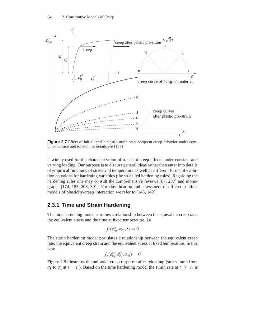
54 2 Constitutive Models of Creep
t
εcrvM
ε
σ
εpl0 ε
pl1
σ 0
σ 1
creep
creep after plastic pre-strain
creep curve of “virgin” material
creep curvesafter plastic pre-strain
σ
√3τ
a
a
b
b
c
c
d
d
e
e
Figure 2.7 Effect of initial tensile plastic strain on subsequent creep behavior under com-bined tension and torsion, for details see [157]
is widely used for the characterization of transient creep effects under constant andvarying loading. Our purpose is to discuss general ideas rather than enter into detailsof empirical functions of stress and temperature as well as different forms of evolu-tion equations for hardening variables (the so-called hardening rules). Regarding thehardening rules one may consult the comprehensive reviews [87, 237] and mono-graphs [174, 185, 208, 301]. For classification and assessment of different unifiedmodels of plasticity-creep interaction we refer to [148, 149].
2.3.1 Time and Strain Hardening
The time hardening model assumes a relationship between theequivalent creep rate,the equivalent stress and the time at fixed temperature, i.e.
ft(εcreq, σeq, t) = 0
The strain hardening model postulates a relationship between the equivalent creeprate, the equivalent creep strain and the equivalent stressat fixed temperature. In thiscase
fs(εcreq, εcr
eq, σeq) = 0
Figure 2.8 illustrates the uni-axial creep response after reloading (stress jump fromσ1 to σ2 at t = tr). Based on the time hardening model the strain rate att ≥ tr is
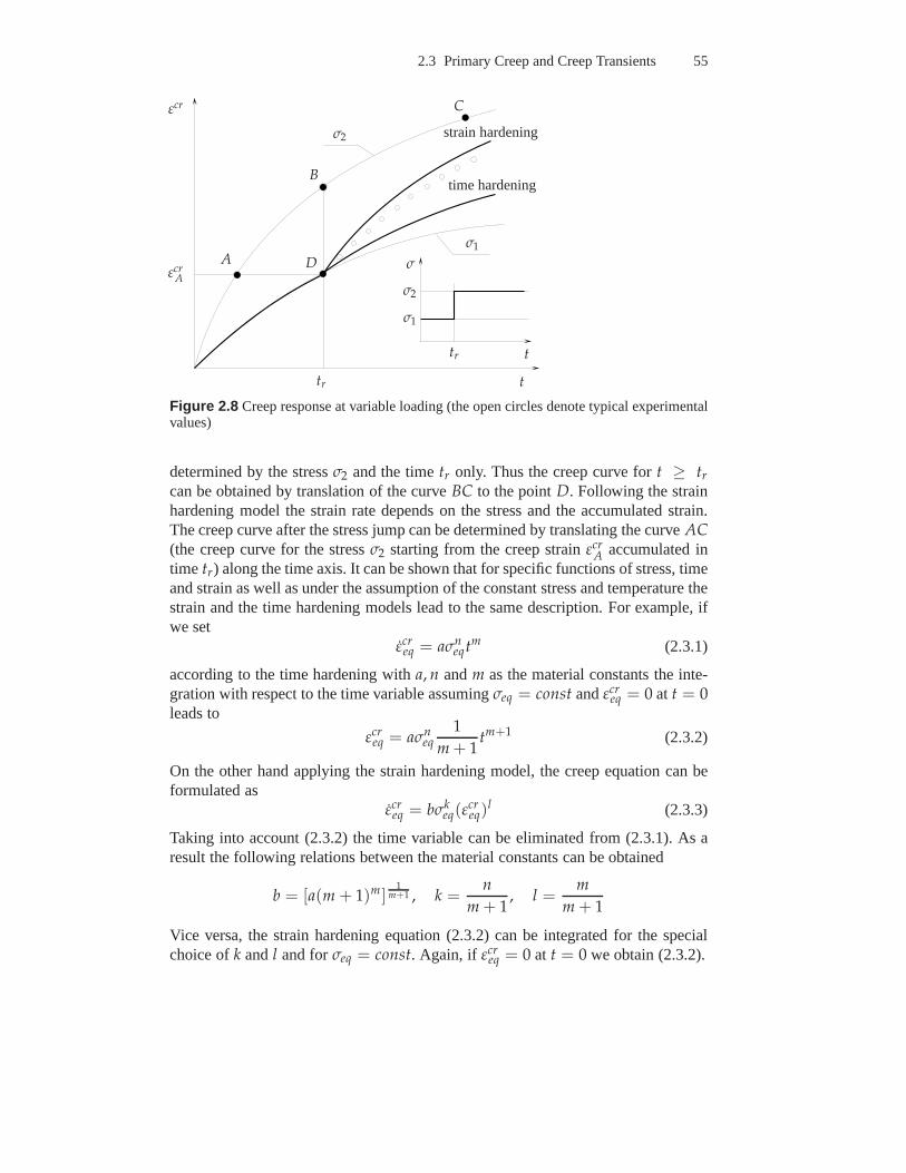
2.3 Primary Creep and Creep Transients 55
replacements
t
t
εcr
A
B
C
tr
tr
εcrA
σ
σ1
σ2
time hardening
strain hardening
σ1
σ2
D
Figure 2.8 Creep response at variable loading (the open circles denotetypical experimentalvalues)
determined by the stressσ2 and the timetr only. Thus the creep curve fort ≥ tr
can be obtained by translation of the curveBC to the pointD. Following the strainhardening model the strain rate depends on the stress and theaccumulated strain.The creep curve after the stress jump can be determined by translating the curveAC(the creep curve for the stressσ2 starting from the creep strainεcr
A accumulated intime tr) along the time axis. It can be shown that for specific functions of stress, timeand strain as well as under the assumption of the constant stress and temperature thestrain and the time hardening models lead to the same description. For example, ifwe set
εcreq = aσn
eqtm (2.3.1)
according to the time hardening witha, n andm as the material constants the inte-gration with respect to the time variable assumingσeq = const andεcr
eq = 0 at t = 0leads to
εcreq = aσn
eq1
m + 1tm+1 (2.3.2)
On the other hand applying the strain hardening model, the creep equation can beformulated as
εcreq = bσk
eq(εcreq)
l (2.3.3)
Taking into account (2.3.2) the time variable can be eliminated from (2.3.1). As aresult the following relations between the material constants can be obtained
b = [a(m + 1)m]1
m+1 , k =n
m + 1, l =
m
m + 1
Vice versa, the strain hardening equation (2.3.2) can be integrated for the specialchoice ofk andl and forσeq = const. Again, if εcr
eq = 0 at t = 0 we obtain (2.3.2).
56 2 Constitutive Models of Creep
Applying the time hardening model the von Mises-Odqvist creep theory (seeSect. 2.2) can be generalized as follows
εεεcr =3
2aσn−1
vM tmsss (2.3.4)
By analogy one can formulate the creep constitutive equation with the strain hard-ening
εεεcr =3
2bσk−1
vM (εcrvM)lsss (2.3.5)
The time and the strain hardening models provide simple empirical descriptionof the uni-axial creep curve within the range of primary creep and are still popularin characterizing the material behavior, e.g. [137, 145, 171]. Despite the simplicity,both the models suffer from significant limitations, even ifapplied stress and tem-perature are constant. The disadvantage of the time hardening model is that the timevariable appears explicitly in equation (2.3.1) for the creep rate. An additional draw-back is that the constantsm andl take usually the values−1 < m < 0, −1 < l < 0as the result of curve fitting. Ifεcr
eq = 0 at t = 0 then Eq. (2.3.3) provides an infinitestarting creep rate. One can avoid this problem in a time-step based numerical pro-cedure assuming a small non-zero creep equivalent strain atthe starting time step.Finally, both models can be applied only for the case of the constant or slowly vary-ing stresses. Transient creep effects under rapid changes of loading and particularlyin the case of stress reversals cannot be described.
Further details of time and strain hardening models can be found in [173, 250].In [173] a modified strain hardening model is proposed based on the idea of creepstrain origins.
2.3.2 Kinematic Hardening
The common approach in describing transient creep effects under complex loadingpaths is the introduction of internal state variables and appropriate evolution equa-tions (the so-called hardening rules). The scalar-valued internal state variables areintroduced in the literature to characterize isotropic hardening and ageing processes.An example will be discussed in Sect. 2.4.1.3. Several “non-classical” effects ob-served in tests under non-proportional loading have motivated the use of tensor-valued variables (usually second rank tensors).
The idea of kinematic hardening (translation of the yield surface in the stressspace) originates from the theory of plasticity and has beenintroduced by Prager[257]. In the creep mechanics the kinematic hardening was proposed by Malininand Khadjinsky [203, 204]. The starting point is the additive decomposition of thestress tensor into two parts:σσσ = σσσ + ααα, whereσσσ is called the active or the effectivepart of the stress tensor andααα denotes the additional or translation part of the stresstensor (back stress tensor). The introduced tensors can be further decomposed intospherical and deviatoric parts
2.3 Primary Creep and Creep Transients 57
σσσ =1
3tr σσσIII + sss, tr sss = 0,
ααα =1
3tr αααIII + βββ, tr βββ = 0,
σσσ =1
3(tr σσσ + tr ααα)III + sss, sss = sss + βββ
(2.3.6)
It is assumed that the inelastic strain rate is determined bythe active part of the stresstensor. The creep potential is then a function of the active part of the stress tensor, i.e.W = W(σσσ) = W(σσσ − ααα), e.g. [245]. As in the case of the classical isotropic creep(Sect. 2.2.1.1) only the second invariant of the deviatorsss is considered. Introducingthe von Mises equivalent stress
σvM ≡√
3
2sss ······ sss =
√
3
2(sss − βββ) ······ (sss − βββ) (2.3.7)
the flow rule (2.1.6) leads to the following constitutive equation
εεεcr =3
2
εcrvM
σvMsss, εvM ≡
√
2
3εεεcr ······ εεεcr (2.3.8)
The equivalent creep rate can be expressed by the use of stress and temperaturefunctions discussed in Sect. 2.2.3. For example, with the power law stress functionand the Arrhenius temperature dependence
εcrvM = aσn
vM, a = a0 exp
(
− Q
RT
)
(2.3.9)
Equations (2.3.8) contain the deviatoric part of the back stressβββ. This internal statevariable is defined by the evolution equation and the initialcondition. In [201, 202]the following evolution equation is postulated
βββ =2
3bεεεcr − g(αvM)
αvMβββ (2.3.10)
with
αvM ≡√
3
2βββ ······ βββ
For the functiong various empirical relations were proposed. One example is [201,202]
g(αvM) = cαnvM, c = c0 exp
(
− Qr
RT
)
Equation (2.3.10) is the multi-axial utilization of the Bailey-Orowan recovery hy-pothesis, see Sect. 2.2.3.b and c0 are material constants andQr is the activationenergy of recovery.
Let us show how the model behaves for the uni-axial homogeneous stress stateσσσ(t) = σ(t)nnn ⊗ nnn, whereσ(t) is the magnitude of the applied stress andnnn is the
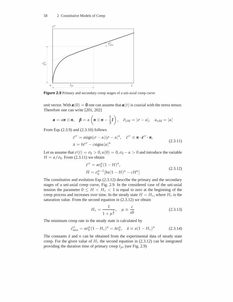
58 2 Constitutive Models of Creep
0 t
εcr
tpr
εcrpr
εcrmin
Figure 2.9 Primary and secondary creep stages of a uni-axial creep curve
unit vector. Withααα(0) = 000 one can assume thatααα(t) is coaxial with the stress tensor.Therefore one can write [201, 202]
ααα = αnnn ⊗ nnn, βββ = α
(
nnn ⊗ nnn − 1
3III
)
, σvM = |σ − α|, αvM = |α|
From Eqs (2.3.9) and (2.3.10) follows
εcr = asign(σ − α)|σ − α|n, εcr ≡ nnn ··· εεεcr ··· nnn,
α = bεcr − csignα|α|n(2.3.11)
Let us assume thatσ(t) = σ0 > 0, α(0) = 0, σ0 − α > 0 and introduce the variableH = α/σ0. From (2.3.11) we obtain
εcr = aσn0 (1 − H)n,
H = σn−10 [ba(1 − H)n − cHn]
(2.3.12)
The constitutive and evolution Eqs (2.3.12) describe the primary and the secondarystages of a uni-axial creep curve, Fig. 2.9. In the considered case of the uni-axialtension the parameter0 ≤ H < H∗ < 1 is equal to zero at the beginning of thecreep process and increases over time. In the steady stateH = H∗, whereH∗ is thesaturation value. From the second equation in (2.3.12) we obtain
H∗ =1
1 + µ1n
, µ ≡ c
ab(2.3.13)
The minimum creep rate in the steady state is calculated by
εcrmin = aσn
0 (1 − H∗)n = aσn0 , a ≡ a(1 − H∗)n (2.3.14)
The constantsa andn can be obtained from the experimental data of steady statecreep. For the given value ofH∗ the second equation in (2.3.12) can be integratedproviding the duration time of primary creeptpr (see Fig. 2.9)
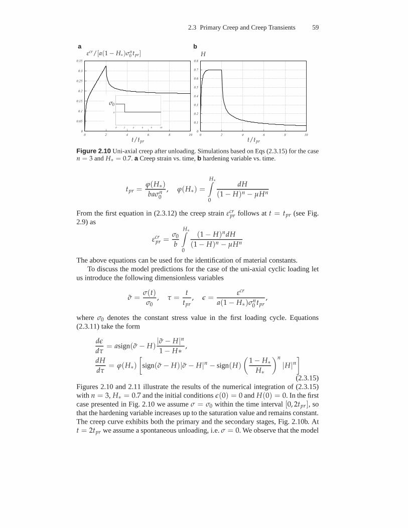
2.3 Primary Creep and Creep Transients 59
0 2 4 6 8 1 00
0 . 0 5
0 . 1
0 . 1 5
0 . 2
0 . 2 5
0 . 3
0 . 3 5
0 2 4 6 8 1 00
0 . 1
0 . 2
0 . 3
0 . 4
0 . 5
0 . 6
0 . 7
0 . 8
0 2 4 6 8 1 0
0
t/tprt/tpr
εcr/[a(1 − H∗)σn0 tpr] H
σ0
a b
Figure 2.10 Uni-axial creep after unloading. Simulations based on Eqs (2.3.15) for the casen = 3 andH∗ = 0.7. a Creep strain vs. time,b hardening variable vs. time.
tpr =ϕ(H∗)baσn
0
, ϕ(H∗) =
H∗∫
0
dH
(1 − H)n − µHn
From the first equation in (2.3.12) the creep strainεcrpr follows at t = tpr (see Fig.
2.9) as
εcrpr =
σ0
b
H∗∫
0
(1 − H)ndH
(1 − H)n − µHn
The above equations can be used for the identification of material constants.To discuss the model predictions for the case of the uni-axial cyclic loading let
us introduce the following dimensionless variables
σ =σ(t)
σ0, τ =
t
tpr, ǫ =
εcr
a(1 − H∗)σn0 tpr
,
where σ0 denotes the constant stress value in the first loading cycle.Equations(2.3.11) take the form
dǫ
dτ= asign(σ − H)
|σ − H|n1 − H∗ ,
dH
dτ= ϕ(H∗)
[
sign(σ − H)|σ − H|n − sign(H)
(
1 − H∗H∗
)n
|H|n]
(2.3.15)Figures 2.10 and 2.11 illustrate the results of the numerical integration of (2.3.15)with n = 3, H∗ = 0.7 and the initial conditionsǫ(0) = 0 andH(0) = 0. In the firstcase presented in Fig. 2.10 we assumeσ = σ0 within the time interval[0, 2tpr ], sothat the hardening variable increases up to the saturation value and remains constant.The creep curve exhibits both the primary and the secondary stages, Fig. 2.10b. Att = 2tpr we assume a spontaneous unloading, i.e.σ = 0. We observe that the model
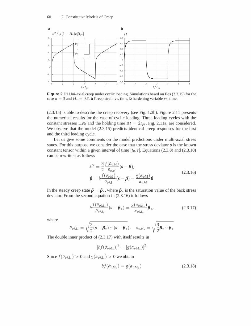
60 2 Constitutive Models of Creep
0 1 2 3 4 5 6- 0 . 2
- 0 . 1
0
0 . 1
0 . 2
0 . 3
0 . 4
0 1 2 3 4 5 6- 0 . 8
- 0 . 6
- 0 . 4
- 0 . 2
0
0 . 2
0 . 4
0 . 6
0 . 8
0 2 4 6
0
t/tprt/tpr
εcr/[a(1 − H∗)σn0 tpr] H
σ0
σ0
a b
Figure 2.11 Uni-axial creep under cyclic loading. Simulations based onEqs (2.3.15) for thecasen = 3 andH∗ = 0.7. a Creep strain vs. time,b hardening variable vs. time.
(2.3.15) is able to describe the creep recovery (see Fig. 1.3b). Figure 2.11 presentsthe numerical results for the case of cyclic loading. Three loading cycles with theconstant stresses±σ0 and the holding time∆t = 2tpr, Fig. 2.11a, are considered.We observe that the model (2.3.15) predicts identical creepresponses for the firstand the third loading cycle.
Let us give some comments on the model predictions under multi-axial stressstates. For this purpose we consider the case that the stressdeviatorsss is the knownconstant tensor within a given interval of time[t0, t]. Equations (2.3.8) and (2.3.10)can be rewritten as follows
εεεcr =3
2
f (σvM)
σvM(sss − βββ),
βββ = bf (σvM)
σvM(sss − βββ)− g(αvM)
αvMβββ
(2.3.16)
In the steady creep stateβββ = βββ∗, whereβββ∗ is the saturation value of the back stressdeviator. From the second equation in (2.3.16) it follows
bf (σvM∗ )
σvM∗(sss − βββ∗) =
g(αvM∗)
αvM∗βββ∗, (2.3.17)
where
σvM∗ =
√
3
2(sss − βββ∗) ······ (sss − βββ∗), αvM∗ =
√
3
2βββ∗ ······ βββ∗
The double inner product of (2.3.17) with itself results in
[b f (σvM∗ )]2 = [g(αvM∗ )]
2
Since f (σvM∗) > 0 andg(αvM∗) > 0 we obtain
b f (σvM∗) = g(αvM∗) (2.3.18)
2.3 Primary Creep and Creep Transients 61
From (2.3.17) it follows
βββ∗ =αvM∗
σvM∗ + αvM∗sss ⇒ σvM∗ = σvM + αvM∗ (2.3.19)
Now the steady state value of the back stress deviator can be calculated
βββ∗ = αvM∗sss
σvM(2.3.20)
Let us assume power functions forf andg. Then from (2.3.18) it follows
ba(σvM − αvM∗)n = cαn
vM∗
As in the uni-axial case we introduce the hardening variableH = αvM/σvM. Thesaturation valueH∗ is then determined by (2.3.13). From the first Eq. in (2.3.16)weobtain
εεεcrst =
3
2aσn−1
vm sss, a ≡ a(1 − H∗)n (2.3.21)
We observe that the kinematic hardening model (2.3.16) results in the classicalNorton-Bailey-Odqvist constitutive equation of steady-state creep discussed in Sect.2.2.1. This model predicts isotropic steady state creep independently from the initialcondition for the back stress deviatorβββ. Furthermore, different stress states leadingto the same value of the von Mises equivalent stress will provide the same steadystate value of the equivalent creep rate.
The model (2.3.16) is applied in [202, 245] for the description of creep for dif-ferent materials under simple or non-proportional loadingconditions. It is demon-strated that the predictions agree with experimental results. However, in many casesdeviations from the Norton-Bailey-Odqvist type steady state creep can be observedin experiments. For example, in the case shown in Fig. 2.6 thesteady state shearcreep rate changes significantly after the shear stress reversals, although the vonMises equivalent stress remains constant. The results presented in Fig. 2.7 indicatethat the initial hardening state due to plastic pre-strain is the reason for the stressstate dependence of the subsequent creep behavior. This effect cannot be describedby the model (2.3.16).
The models with the back stress of the type (2.3.16) are usually termed to bethe models with anisotropic hardening, e.g. [202]. The typeof anisotropy is thendetermined by the symmetry group of the back stress tensor ordeviator. The sym-metry group of any symmetric second rank tensor includes always nine elements,e.g. [199]. For the tensorβββ the symmetry elements are
QQQβββ = ±nnn1 ⊗ nnn1 ± nnn2 ⊗ nnn2 ± nnn3 ⊗ nnn3, (2.3.22)
wherennni are the principal axes. In order to verify the assumed symmetries of hard-ening one should perform creep tests with non-proportionalloading of the followingtype. During the first cycle a homogeneous constant stress state with the deviatoricpartsss should be applied over a period of time[0, t1], t1 < tpr. During the second
62 2 Constitutive Models of Creep
loading cycle the stress statesQQQi ··· sss ··· QQQTi should be applied, where the orthogonal
tensorsQQQi do not belong to the symmetry group ofsss. Among all stress states of thistype the stress statesQQQβββ ··· sss ··· QQQT
βββ should exist leading to the same (with respect tothe scatter of experimental data) creep response after reloading.
As shown in [72] kinematic hardening of the type (2.3.16) leads to a restrictiveform of orthotropic inelastic behavior. In order to demonstrate this let us write downthe back stress deviator in the following form
βββ = β1nnn1 ⊗ nnn1 + β2nnn2 ⊗ nnn2 − (β1 + β2)nnn3 ⊗ nnn3
= β1(nnn1 ⊗ nnn1 − nnn3 ⊗ nnn3) + β2(nnn2 ⊗ nnn2 − nnn3 ⊗ nnn3),
whereβ1 andβ2 are the principal values andnnn1, nnn2 andnnn3 are the principal direc-tions ofβββ. For the given back stress deviatorβββ the equivalent stress (2.3.7) takes theform
σ2vM = 3 J2
1
(
1 − β1
J1
)2
+ 3 J22
(
1 − β2
J2
)2
+3
2J1 J2
(
1 − β1
J1
)(
1 − β2
J2
)
+ 3I2nnn1nnn2
+ 3I2nnn1nnn3
+ 3I2nnn2nnn3
,(2.3.23)
where the invariantsJi are defined by Eqs (2.2.53) and the invariantsInnninnnjare defined
by Eqs (2.2.48). Steady state creep with initial orthotropic symmetry is discussed inSect. 2.2.2. In this case the von Mises type equivalent stress includes 6 invariantsand 6 independent material constants. The equivalent stress (2.3.23) contains all6 orthotropic invariants. However, the last three terms (three shear stresses withrespect to the three planes of the orthotropic symmetry) arenot affected by thehardening. Furthermore, in the steady state range these terms vanish since the backstress deviatorβββ∗ is coaxial with the stress deviator according to (2.3.20).
The possibilities to improve the predictions of the kinematic hardening modelare:
– Introduction of additional state variables like isotropichardening variable, e.g.[87], ageing variable, e.g. [238], or damage variables, e.g. [101]. Models withdamage variables will be discussed in Sect. 2.4.
– Formulation of the creep potential as a general isotropic function of two tensorsσσσandααα. Such an approach is proposed in [72] for the case of plasticity and includesdifferent special cases of kinematic hardening,
– Consideration of the initial anisotropy of the material behavior, e.g. [148].
Creep models with kinematic hardening of the type (2.3.8) and different specificforms of the hardening evolution equation are discussed in [158, 159, 202, 238, 245,272] among others. For the description of creep and creep-plasticity interaction atcomplex loading conditions a variety of unified models is available including thehardening variables as second rank tensors. For details we refer to [174, 176, 185,208]. Several unified models are reviewed and evaluated in [148, 149]. The historicalbackground of the development of non-linear kinematic hardening rules is presentedin [87].
2.4 Tertiary Creep and Creep Damage 63
2.4 Tertiary Creep and Creep Damage
Tertiary creep stage is the final part of the creep process. Ina uni-axial creep curvetertiary creep is observed as the increase of the creep rate.The shape of the finalpart of the creep curve and the duration of the tertiary creepdepends on the materialcomposition, the stress level and the temperature. For somestructural steels, thetertiary creep is the major part of the whole creep process, e.g. [105, 242].
The origins of tertiary creep are progressive damage processes including theformation, growth and coalescence of voids on grain boundaries, coarsening of pre-cipitates and environmental effects. The voids may nucleate earlier during the creepprocess, possibly at primary creep stage or even after spontaneous deformation. Theinitially existing micro-defects have negligible influence on the creep rate. As theirnumber and size increase with time, they weaken the materialproviding the de-crease in the load-bearing capacity. The coalescence of cavities or propagation ofmicro-cracks lead to the final fracture. Creep fracture is usually inter-granular [33].Dyson [99] distinguishes three main categories of creep damage: the strain induceddamage, the thermally induced damage and the environmentally induced damage.The strain induced damage may be classified as follows [101]
– excessive straining at constant load,– grain boundary cavitation and– progressive multiplication of the dislocation substructure
The first two damage mechanisms occur in all poly-crystalline materials, whereasthe third one is essential for nickel-based super-alloys.
The thermally induced damage mechanisms include material ageing processeswhich lead to the loss of strength and contribute to the nucleation and growth ofcavities. The example of the thermally induced ageing includes the coarsening ofcarbide precipitates for ferritic steels (increase of volume fraction of carbide precip-itates or new precipitation), e.g. [251]. The rate of ageingdoes not depend on theapplied stress, but is influenced by the temperature and can be identified by exposingtest-pieces to thermal environment.
The environmentally induced damage (corrosion, oxidation, etc.) appears dueto the attack of chemical species contained within the surrounding medium. Theenvironmental damage rate can be inversely related to the test-piece (component)dimensions [99].
The dominance of a creep damage mechanism depends on the alloy composi-tion, on the fabrication route and on the service conditions. For several metals andalloys, fracture mechanism maps are available [33]. By analogy with the deforma-tion mechanism maps, regions with different fracture modesare indicated dependingon the stress and the temperature ranges.
Physical modeling of creep damage is complicated by the factthat many differ-ent mechanisms may operate and interact in a specific material under given loadingconditions. This interaction should be taken into account in the damage rate equa-tions. Models related to the grain boundary cavitation are discussed and reviewed in[155, 271].
64 2 Constitutive Models of Creep
The characterization of tertiary creep under multi-axial stress states is the im-portant step in a creep analysis of engineering structures.A lifetime prediction of aspecific load bearing component designed for creep, or a residual lifetime estima-tion of a structure operating at elevated temperature requires a model which takesinto account tertiary creep and damage evolution under multi-axial stress states.
The damage rate and consequently the creep rate are determined by the stresslevel, the accumulated damage and the temperature. These dependencies can be es-tablished based on experimental data from the uni-axial creep testing. If the materialis subjected to multi-axial loading, the kind of stress state has a significant influenceon the damage growth. Tension and compression lead to different creep rates. Dif-ferent stress states corresponding to the same von Mises equivalent stress lead, ingeneral, to different equivalent tertiary creep rates while the equivalent strain rate inthe secondary stage is approximately the same. These facts are established from thedata of creep tests under combined tension and torsion, e.g.[169, 170], as well asfrom biaxial and triaxial creep tests [282, 283]. Stress state effects must be consid-ered in the damage evolution equation. In Sect. 2.4.1 we discuss various possibilitiesto characterize the tertiary creep behavior by means of scalar valued damage para-meters. Under non-proportional loading conditions, the additional factor is the in-fluence of the damage induced anisotropy. Examples are creeptests under combinedtension and alternating torsion, e.g. [218], and creep tests under biaxial loading withalternating direction of the first principal stress [283]. In both cases the assumptionof isotropic creep behavior and the scalar measure of damagelead to disagreementwith experimental observations. In Sect. 2.4.2 we review some experimental resultsillustrating the damage induced anisotropy and discuss creep-damage models withtensor-valued damage variables.
2.4.1 Scalar-Valued Damage Variables
Many microstructural observations show the directional effect of creep damage. Forexample, during a cyclic torsion test on copper voids nucleate and grow predomi-nantly on those grain boundaries, which are perpendicular to the first principal di-rection of the stress tensor, e.g. [134]. Creep damage has therefore an anisotropicnature and should be characterized by a tensor. However, if the initially isotropicmaterial is subjected to constant or monotonic loading the influence of the damageanisotropy on the observed creep behavior, i.e. the strain vs. time curves, is not sig-nificant. If the state of damage is characterized by a tensor (see Sect. 2.4.2) then sucha tensor can be assumed to be coaxial with the stress tensor under monotonic loadingconditions. In such a case only the scalar damage measures will enter the creep con-stitutive equation. Below we introduce different models oftertiary creep includingthe phenomenological, the so-called micromechanically consistent and mechanismbased models. The effect of damage is described by means of scalar valued damageparameters and corresponding evolution equations. The stress state influences areexpressed in the equivalent stress responsible for the damage evolution.2.4.1.1 Kachanov-Rabotnov Model. The phenomenological creep-damageequations were firstly proposed by L. Kachanov [150] and Rabotnov [263]. A new
2.4 Tertiary Creep and Creep Damage 65
internal variable has been introduced to characterize the “continuity” or the “dam-age” of the material. The geometrical interpretation of thecontinuity variable startsfrom changes in the cross-section area of a uni-axial specimen. Specifying the initialcross-section area of a specimen byA0 and the area of voids, cavities, micro-cracks,etc. byAD, the Kachanov’s continuity is defined as follows (see [152])
ψ =A0 − AD
A0
The valueψ = 1 means the virgin, fully undamaged state, the conditionψ = 0corresponds to the fracture (completely damaged cross-section).
Rabotnov [263, 264, 265] introduced the dual damage variable ω. In [264] hepointed out that the damage state variableω “may be associated with the area frac-tion of cracks, but such an interpretation is connected witha rough scheme and istherefore not necessary”. Rabotnov assumed that the creep rate is additionally de-pendent on the current damage state. The constitutive equation should have the form
εcr = εcr(σ, ω)
Furthermore, the damage processes can be reflected in the evolution equation
ω = ω(σ, ω), ω|t=0 = 0, ω < ω∗,
whereω∗ is the critical value of the damage parameter for which the material fails.With the power functions of stress and damage the constitutive equation may beformulated as follows
εcr =aσn
(1 − ω)m(2.4.1)
Similarly, the damage rate can be expressed by
ω =bσk
(1 − ω)l(2.4.2)
These equations contain the material dependent constants:a, b, n, m, l, k. It is easyto prove that for the damage free state (ω = 0), the first equation results in thepower law creep constitutive equation.
Settingm = n the first equation can be written as
εcr = aσn, (2.4.3)
where σ = σ/(1 − ω) is the so-called net-stress or effective stress. In this case(2.4.3) is a generalization of the Norton-Bailey secondarycreep law for the descrip-tion of tertiary creep process. Lemaitre and Chaboche [185]proposed the effectivestress concept to formulate constitutive equations for damaged materials based onavailable constitutive equation for “virgin” materials. An interpretation can be givenfor a tension bar, Fig. 2.12. HereA0 denotes the initial cross-section area of the bar,Fig. 2.12a. From the given tensile forceF the stress can be computed asσ = F/A0.
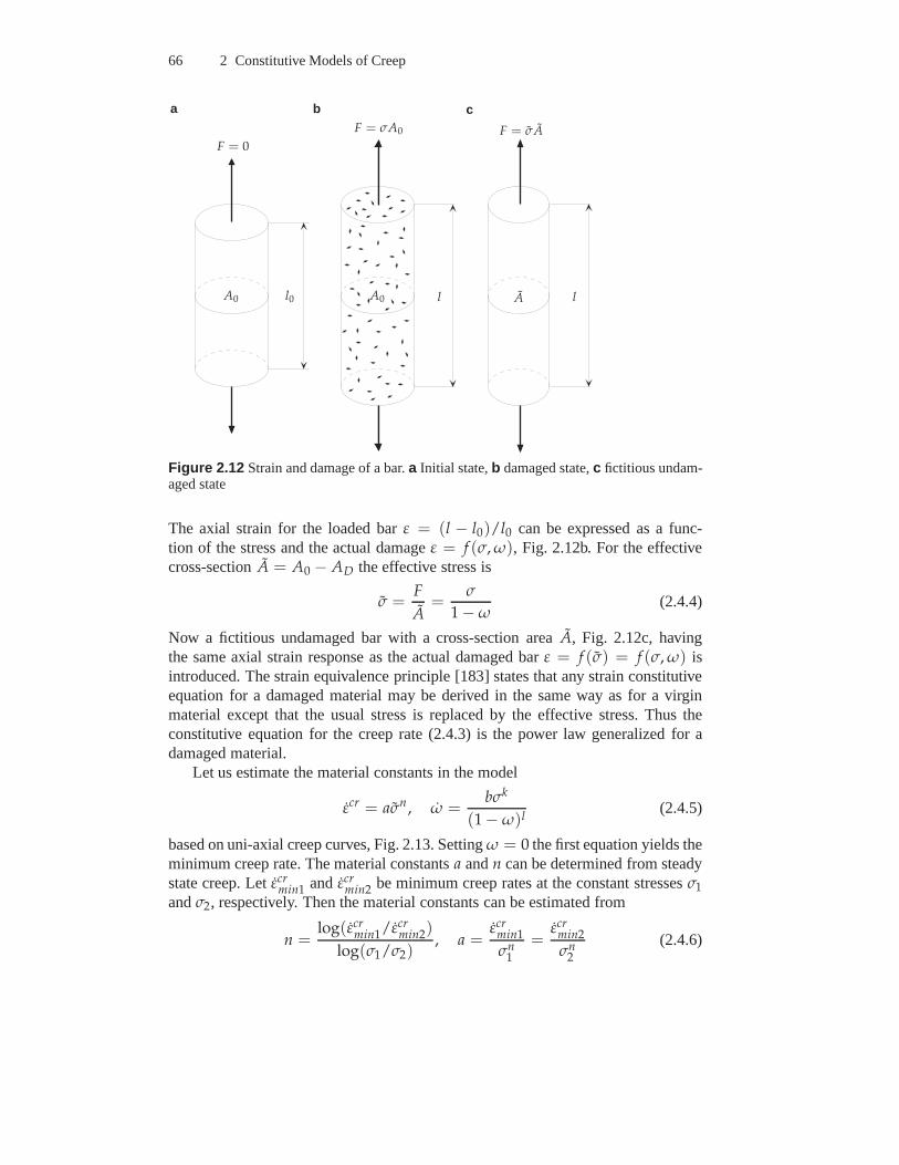
66 2 Constitutive Models of Creep
F = 0
A0 l0
F = σA0
A0
F = σA
A ll
a b c
Figure 2.12 Strain and damage of a bar.a Initial state,b damaged state,c fictitious undam-aged state
The axial strain for the loaded barε = (l − l0)/l0 can be expressed as a func-tion of the stress and the actual damageε = f (σ, ω), Fig. 2.12b. For the effectivecross-sectionA = A0 − AD the effective stress is
σ =F
A=
σ
1 − ω(2.4.4)
Now a fictitious undamaged bar with a cross-section areaA, Fig. 2.12c, havingthe same axial strain response as the actual damaged barε = f (σ) = f (σ, ω) isintroduced. The strain equivalence principle [183] statesthat any strain constitutiveequation for a damaged material may be derived in the same wayas for a virginmaterial except that the usual stress is replaced by the effective stress. Thus theconstitutive equation for the creep rate (2.4.3) is the power law generalized for adamaged material.
Let us estimate the material constants in the model
εcr = aσn, ω =bσk
(1 − ω)l(2.4.5)
based on uni-axial creep curves, Fig. 2.13. Settingω = 0 the first equation yields theminimum creep rate. The material constantsa andn can be determined from steadystate creep. Letεcr
min1 and εcrmin2 be minimum creep rates at the constant stressesσ1
andσ2, respectively. Then the material constants can be estimated from
n =log(εcr
min1/εcrmin2)
log(σ1/σ2), a =
εcrmin1
σn1
=εcr
min2
σn2
(2.4.6)
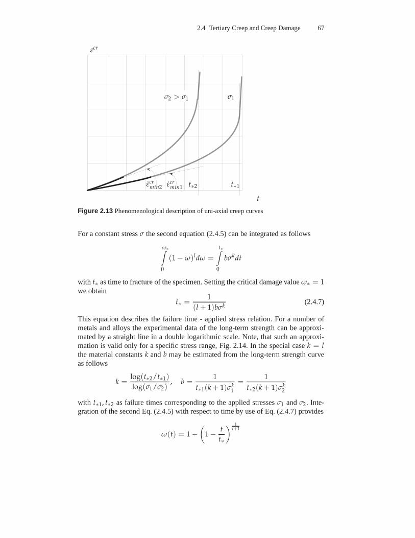
2.4 Tertiary Creep and Creep Damage 67
t
t∗2 t∗1εcrmin2 εcr
min1
σ1σ2 > σ1
εcr
Figure 2.13 Phenomenological description of uni-axial creep curves
For a constant stressσ the second equation (2.4.5) can be integrated as follows
ω∗∫
0
(1 − ω)ldω =
t∗∫
0
bσkdt
with t∗ as time to fracture of the specimen. Setting the critical damage valueω∗ = 1we obtain
t∗ =1
(l + 1)bσk(2.4.7)
This equation describes the failure time - applied stress relation. For a number ofmetals and alloys the experimental data of the long-term strength can be approxi-mated by a straight line in a double logarithmic scale. Note,that such an approxi-mation is valid only for a specific stress range, Fig. 2.14. Inthe special casek = lthe material constantsk andb may be estimated from the long-term strength curveas follows
k =log(t∗2/t∗1)
log(σ1/σ2), b =
1
t∗1(k + 1)σk1
=1
t∗2(k + 1)σk2
with t∗1, t∗2 as failure times corresponding to the applied stressesσ1 andσ2. Inte-gration of the second Eq. (2.4.5) with respect to time by use of Eq. (2.4.7) provides
ω(t) = 1 −(
1 − t
t∗
) 1l+1
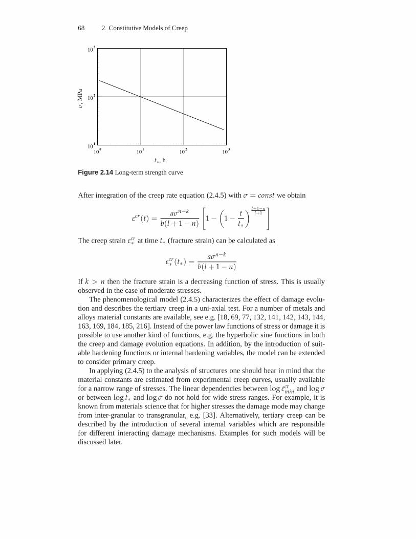
68 2 Constitutive Models of Creep
100
101
102
103
101
102
103
t∗, h
σ,M
Pa
Figure 2.14 Long-term strength curve
After integration of the creep rate equation (2.4.5) withσ = const we obtain
εcr(t) =aσn−k
b(l + 1 − n)
[
1 −(
1 − t
t∗
) l+1−nl+1
]
The creep strainεcr∗ at timet∗ (fracture strain) can be calculated as
εcr∗ (t∗) =
aσn−k
b(l + 1 − n)
If k > n then the fracture strain is a decreasing function of stress.This is usuallyobserved in the case of moderate stresses.
The phenomenological model (2.4.5) characterizes the effect of damage evolu-tion and describes the tertiary creep in a uni-axial test. For a number of metals andalloys material constants are available, see e.g. [18, 69, 77, 132, 141, 142, 143, 144,163, 169, 184, 185, 216]. Instead of the power law functions of stress or damage it ispossible to use another kind of functions, e.g. the hyperbolic sine functions in boththe creep and damage evolution equations. In addition, by the introduction of suit-able hardening functions or internal hardening variables,the model can be extendedto consider primary creep.
In applying (2.4.5) to the analysis of structures one shouldbear in mind that thematerial constants are estimated from experimental creep curves, usually availablefor a narrow range of stresses. The linear dependencies betweenlog εcr
min andlog σor betweenlog t∗ and log σ do not hold for wide stress ranges. For example, it isknown from materials science that for higher stresses the damage mode may changefrom inter-granular to transgranular, e.g. [33]. Alternatively, tertiary creep can bedescribed by the introduction of several internal variables which are responsiblefor different interacting damage mechanisms. Examples forsuch models will bediscussed later.
2.4 Tertiary Creep and Creep Damage 69
The model (2.4.5) is a system of two ordinary differential equations, which mustbe integrated over time in order to obtain the current creep strain and damage. Forthe analysis of statically indeterminate structures the integration must be performednumerically, even in the case of a uni-axial stress state. Insome cases the effect oftertiary creep rate does not lead to significant stress redistribution and one can ne-glect the damage variable in the constitutive equation (2.4.1), e.g. [276]. The dam-age evolution equation can be integrated separately providing the time to fractureestimation for the given constant stress in the steady-state creep range.
To discuss multi-axial versions of (2.4.1) and (2.4.2) let us neglect primary creepeffects and assume the von Mises type secondary creep material model introducedin Sect. 2.2.1
εεεcr =3
2aσn
vMsss
σvM(2.4.8)
Rabotnov [264] assumed that the the creep potential for the damaged material hasthe same form as for the secondary creep. His proposition wasthe introduction ofan effective stress tensorσσσ = fff (σσσ, ω). For the case of distinct principal values ofthe stress tensorσI > σI I > σI I I andσI > 0 the following expression is suggested[264]
σσσ =σI
1 − ωnnnI ⊗ nnnI + σI InnnI I ⊗ nnnI I + σI I InnnI I I ⊗ nnnI I I
If we apply the strain equivalence principle [185] than the constitutive equation(2.4.8) can be modified by replacing the stress tensorσσσ with the effective one. As-suming the effective stress tensor in the formσσσ = σσσ/(1 − ω), the constitutiveequation (2.4.8) can be generalized as follows [182]
εεεcr =3
2a
(
σvM
1 − ω
)n sss
σvM(2.4.9)
The next step is the formulation of the damage evolution equation. By analogy withthe uni-axial case, the damage rate should have a form
ω = ω(σσσ, ω)
The dependence on the stress tensor can be expressed by meansof the “damageequivalent stress”σω
eq(σσσ) which allows to compare tertiary creep and long termstrength under different stress states. With the damage equivalent stress, the uni-axial equation (2.4.2) can be generalized as follows
ω =b(σω
eq)k
(1 − ω)l(2.4.10)
The material constantsa, b, n, k andl can be identified from uni-axial creep curves.In order to find a suitable expression for the damage equivalent stress, the data frommulti-axial creep tests up to rupture are required. In general, σω
eq can be formulatedin terms of three invariants of the stress tensor, for example the basic invariants (seeSect. 2.2.1)
70 2 Constitutive Models of Creep
σωeq = σω
eq[I1(σσσ), I2(σσσ), I3(σσσ)]
Similarly to the uni-axial case, see Eq. (2.4.7), the damageevolution equation(2.4.10) can be integrated assuming that the stress tensor is a constant function oftime. As a result, the relationship between the time to creepfracture and the equiv-alent stress can be obtained
t∗ =1
(l + 1)b(σω
eq)−k (2.4.11)
Sdobyrev [288] carried out long-term tests on tubular specimens made from alloysEI-237B (Ni-based alloy) and EI-405 (Fe-based alloy) undertension, torsion andcombined tension-torsion. The results of the tests are summarized for different tem-peratures with the help of equivalent stress vs. fracture time plots. The followingdependence was established
1
2(σI + σvM) = f (log t∗) (2.4.12)
He found that the linear functionf provides a satisfactory description of the ex-perimental results. The equivalent stress responsible to the long term strength atelevated temperatures is thenσ∗
eq = 12 (σI + σvM). Based on different mechanisms
which control creep failure, the influence of three stress state parameters (the meanstressσm = I1/3, the first positive principal stress or the maximum tensile stressσmaxt = (σI + |σI |)/2 and the von Mises stress) is discussed by Trunin in [314].The Sdobyrev criterion was extended as follows
σ∗eq =
1
2(σvM + σmaxt) a1−2η , η =
3σm
σvM + σmaxt, (2.4.13)
wherea is a material constant. For special loading cases this equivalent stress yields
– uni-axial tension
σ∗eq = σ, η =
1
2
– uni-axial compression
σ∗eq =
σa3
2, η = −1
– pure torsion
σ∗eq =
√3 + 1
2τa, η = 0
The constanta can be calculated from the ultimate stress values leading tothe samefracture time for a given temperature. For example, if the ultimate tension and shearstresses areσu andτu, respectively, then
a =2√
3 + 1
σu
τu
2.4 Tertiary Creep and Creep Damage 71
Hayhurst [132] proposed the following relationship
t∗ = A(ασmaxt + βI1 + γσvM)−χ, (2.4.14)
whereA andχ are material constants,I1 = 3σm andα + β + γ = 1. Comparingthis equation with Eq. (2.4.11) one can obtain
A =1
(l + 1)b, χ = k, σω
eq = ασmaxt + βI1 + γσvM (2.4.15)
Hayhurst introduced the normalized stress tensorσσσ = σσσ/σ0 and the normalizedtime to fracturet∗ = t∗/t∗0, wheret∗0 is the time to fracture in a uni-axial testconducted at the stressσ0. From Eqs (2.4.7) and (2.4.11) it follows
t∗ =
(
σωeq
σ0
)−k
= (σωeq)
−k
By setting the normalized rupture time equal to unity, the equationσωeq = 1 follows,
which is connecting the stress states leading to the equal rupture time. In [132]the data of biaxial tests (biaxial tension test, combined tension and torsion of tubu-lar specimens) for different materials are summarized. It was found convenient topresent the results in terms of the isochronous rupture surface, which is the plot ofthe equationσω
eq = 1 for the specified values ofα and β in the normalized stressspace. For plane stress states the isochronous rupture locican be presented in thenormalized principal stress axes. Examples for different materials are presented in[132]. The coefficientsα andβ are specific for each material and, in addition, theymay depend on the temperature. Figure 2.15 shows the isochronous rupture loci forthree special cases:σω
eq = σmaxt, σωeq = σvM andσω
eq = 3σm. The first two representthe extremes of the material behavior [182].
A more general expression for the damage equivalent stress can be formulatedby the use of three invariants of the stress tensor. With the first invariantI1, the vonMises equivalent stressσvM and
sin 3ξ = −27
2
(s · ss · ss · s) ······ sss
σ3vM
, −π
6≤ ξ ≤ π
6,
as a cubic invariant, the following equivalent stress has been proposed in [27]
σωeq = λ1σvM sin ξ + λ2σvM cos ξ + λ3σvM + λ4 I1 + λ5 I1 sin ξ + λ6 I1 cos ξ
(2.4.16)The identification of coefficientsλi, i = 1, . . . , 6 requires six independent tests.Equation (2.4.16) contains a number of known failure criteria as special cases, see[27]. For example, settingλ1 = λ2 = λ4 = λ5 = λ6 = 0 the equation providesthe von Mises equivalent stress. Taking into account
σI =1
3
[
2σvM sin
(
ξ +2π
3
)
+ I1
]
= −1
3σvM sin ξ +
√3
3σvM cos ξ +
1
3I1
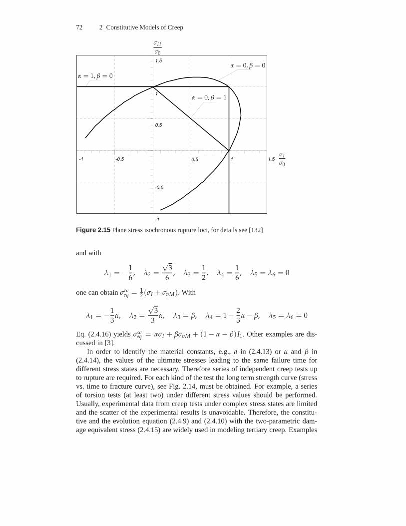
72 2 Constitutive Models of Creep
-1 -0.5 0.5 1 1.5
-1
-0.5
0.5
1
1.5
σI
σ0
σI I
σ0
α = 1, β = 0
α = 0, β = 0
α = 0, β = 1
Figure 2.15 Plane stress isochronous rupture loci, for details see [132]
and with
λ1 = −1
6, λ2 =
√3
6, λ3 =
1
2, λ4 =
1
6, λ5 = λ6 = 0
one can obtainσωeq = 1
2 (σI + σvM). With
λ1 = −1
3α, λ2 =
√3
3α, λ3 = β, λ4 = 1 − 2
3α − β, λ5 = λ6 = 0
Eq. (2.4.16) yieldsσωeq = ασI + βσvM + (1 − α − β)I1. Other examples are dis-
cussed in [3].In order to identify the material constants, e.g.,a in (2.4.13) orα and β in
(2.4.14), the values of the ultimate stresses leading to thesame failure time fordifferent stress states are necessary. Therefore series ofindependent creep tests upto rupture are required. For each kind of the test the long term strength curve (stressvs. time to fracture curve), see Fig. 2.14, must be obtained.For example, a seriesof torsion tests (at least two) under different stress values should be performed.Usually, experimental data from creep tests under complex stress states are limitedand the scatter of the experimental results is unavoidable.Therefore, the constitu-tive and the evolution equation (2.4.9) and (2.4.10) with the two-parametric dam-age equivalent stress (2.4.15) are widely used in modeling tertiary creep. Examples
2.4 Tertiary Creep and Creep Damage 73
of material constants as well as structural mechanics applications can be found in[18, 69, 77, 132, 142, 143, 144, 163, 169] among others.
2.4.1.2 Micromechanically-Consistent Models. The creep constitutiveequation (2.4.9) includes the effect of damage by means of the equivalent stressconcept. An alternative approach to formulate the creep constitutive equation canbe based on micromechanics. Rodin and Parks [277] considered an infinite blockfrom incompressible isotropic material containing a givendistribution of cracks andsubjected to a far field homogeneous stress. As a measure of damage they usedρ = a3N/V, whereN is the number of cracks (voids) in a volumeV anda is theaveraged radius of a crack. Assuming power law creep, they found that the creeppotential for such a material has the following form
W(σσσ, ρ, n) =ε0σ0
n + 1f(
ζ(σσσ), ρ, n)
(
σvM
σ0
)n+1
, (2.4.17)
where ε0 is the reference creep rate,σ0 is the reference stress andn is a materialconstant.ζ(σσσ) is a function representing the influence of the kind of stressstate. In[277] the following particular expression is proposed
ζ(σσσ) =σI
σvM,
whereσI is the maximum principal stress. The creep potential (2.4.17) and the flowrule (2.1.6) give
εεεcr =∂W
∂σσσ=
∂W
∂σvM
∂σvM
∂σσσ+
∂W
∂ζ
∂ζ
∂σσσ
= ε0
(
σvM
σ0
)n [3
2
(
f − ζ f,ζ
n + 1
)
sss
σvM+
f,ζ
n + 1nnnI ⊗ nnnI
]
,
(2.4.18)
wherennnI is the first principal direction of the stress tensor. The function f mustsatisfy the following convexity condition [277]
f f,ζζ −n
n + 1f 2,ζ > 0,
The form of the functionf is established for the assumed particular distribution ofcracks and by use of a self-consistent approach. In [278] thefollowing expression isproposed
f (ζ, ρ, n) =[
1 + α(ρ, n)ζ2] n+1
2,
α(ρ, n) =2ρ
n + 1+
(2n + 3)ρ2
n(n + 1)2+
(n + 3)ρ3
9n(n + 1)3+
(n + 3)ρ4
108n(n + 1)4
Models of the type (2.4.18) are popular in materials sciencerelated literature,e.g. [121, 211]. They are based on micromechanical considerations and therefore
74 2 Constitutive Models of Creep
seem to be more preferable for creep-damage analysis. However, only idealizeddamage states, e.g. dilute non-interacting cracks or voidswith a given densityand specific distribution can be considered. Furthermore, at present there is nomicromechanically-consistent way to establish the form ofthe evolution equationfor the assumed damage variable. Different empirical equations are proposed in theliterature. For example, Mohrmann and Sester [211] assume that the cavity nucle-ation is strain controlled and recommend the following equation
ρ
ρ f=
(
εvM
ε f
)γ
,
whereρ f , ε f andγ are material constants which should be identified from “macro-scopic” creep responses.
Bassani and Hawk [36] proposed to use a phenomenological damage parameterω (see Sect. 2.4.1.1) instead ofρ. The functionf is then postulated as follows
f (ζ, ω, n) =1
(1 − ω)k
(
1 − α0ω + α0ωζ2) n+1
2(2.4.19)
Hereζ = (1 − α1)
σI
σvM+ α1
σH
σvM
andk, n, α0 andα1 are material constants. From Eqs (2.4.18) and (2.4.19) follows
εεεcr = ε0
(
σvM
σ0
)n 1
(1 − ω)k(1 − α0ω + α0ωζ2)
n−12 ×
×
3
2(1 − α0ω)
sss
σvM+ α0ωζ[(1 − α1)nnnI ⊗ nnnI + α1III]
(2.4.20)
With α0 = 1 andk = n (2.4.20) yields the Kachanov-Rabotnov type constitutiveequation (2.4.9). By settingα0 = 1, k = (n + 1)/2 and ω ≪ 1 Eq. (2.4.20)approximates the Rodin and Parks micro-mechanical based model [277]. For thecasek = n, α0 = 1 andα1 = 1 the constitutive equation for the creep rate can bepresented as follows
εεεcr = ε0
[
σvM
σ0(1 − ω)
]n
(1 − ω + ωζ2)n−1
2
[
3
2(1 − ω)
sss
σvM+ ωζIII
]
From Eq. (2.4.20) one can calculate the volumetric creep rate
εV = tr εεεcr = ε0
(
σvM
σ0
)n 1
(1 − ω)k(1 − α0ω + α0ωζ2)
n−12 [α0ωζ(1 + 2α1)]
We observe that the damage growth induces dilatation. Creepconstitutive equations(2.4.18) or (2.4.20) include the first principal dyad of the stress tensor. It should benoted that the dyadnnnI ⊗ nnnI can be found only ifσI 6= 0, σI 6= σI I andσI 6= σI I I .In this case, e.g. [199]
2.4 Tertiary Creep and Creep Damage 75
nnnI ⊗ nnnI =1
(σI − σI I)(σI − σI I I)
[
σσσ2 − (tr σσσ − σI)σσσ +detσσσ
σIIII
]
(2.4.21)
Inserting (2.4.21) into (2.4.18) or into (2.4.20) we observe that not only the volumet-ric strain but also second order effects (see Sect. 2.2.1 fordiscussion) are “induced”by damage.
2.4.1.3 Mechanism-Based Models. The constitutive and evolution equations(2.4.9) and (2.4.10) are formulated in terms of power law functions of stress. Itis known from materials science that the power law creep model guarantees thecorrect description only for a specific stress range (see Sect 2.2.3). In addition, thepower law stress and damage functions used in Eqs. (2.4.9) and (2.4.10) may lead tonumerical problems in finite element simulations of creep instructures with stressconcentrations or in attempts to predict the creep crack growth [192, 281].
The uni-axial creep tests are usually performed under increased stress and tem-perature levels in order to accelerate the creep process. For the long term analysisof structures the material model should be able to predict creep rates for wide stressranges including moderate and small stresses. Within the materials science manydifferent damage mechanisms which may operate depending onthe stress level andthe temperature are discussed, e.g., [99]. Each of the damage mechanisms can beconsidered by a state variable with an appropriate kinetic equation.
Another way for the formulation of a creep-damage constitutive model is theso-called mechanism-based approach. The internal state variables are introducedaccording to those creep and damage mechanisms which dominate for a specificmaterial and specific loading conditions. Furthermore, different functions of stressand temperature proposed in materials science can be utilized. The form and thevalidity frame of such a function depend on many factors including the stress andtemperature levels, type of alloying, grain size, etc. The materials science formula-tions do not provide the values of material constants (only the bounds are given).They must be identified from the data of standard tests, e.g. uni-axial creep test.Examples of mechanism-based models can be found in [133, 134, 171, 243, 251].Here we discuss the model proposed by Perrin and Hayhurst in [251] for a 0.5Cr-0.5Mo-0.25V ferritic steel in the temperature range 600 – 675C.
The starting point is the assumption that the rate of the local grain boundarydeformation is approximately a constant fraction of the overall deformation rate.From this follows that the constitutive equations for the overall creep rate can beformulated in terms of empirical relationships between thelocal grain boundarydeformation rate and the stress, the temperature, the cavitation rate, etc.
For ferritic steels the nucleation of cavities has been observed at carbide particleson grain boundaries due to the local accumulation of dislocations. The nucleationkinetics can be therefore related to the local deformation.Furthermore, the cavitynucleation depends on the stress state characterized byσI/σvM. Cane [83] observedthat the area fraction of intergranular cavities in the plane normal to the appliedstress increases uniformly with the accumulated creep strain. He proposed that thenucleation and growth can be combined into an overall measure of cavitation. Thecavitated area fractionA f can be related to the von Mises equivalent creep strain,
76 2 Constitutive Models of Creep
the von Mises equivalent stress and the maximum principal stress by the equation
A f = DεvM
(
σI
σvM
)µ
, (2.4.22)
whereD andµ are constants depending on the material microstructure. Perrin andHayhurst define the damage state variableω as the cavitated area fraction. The fail-ure condition in a uni-axial creep test is the complete cavitation of all grain bound-aries normal to the applied stress. The cavitated area fraction of such cavities atfailure is approximately1/3. Therefore, the critical state at which the material fails,can be characterized byω∗ = 1/3.
The important mechanism of creep damage for the ferritic steel under consid-eration is the temperature dependent coarsening of carbideprecipitates. First, thecarbide precipitates restrict the deformation of the graininterior and second, theyprovide sites for nucleation of cavities. Following Dyson [99], the particle coars-ening can be characterized by the state variableφ = 1 − li/l related to the initial(li) and current(l) spacing of precipitates. The kinetic equation is derived from thecoarsening theory [99, 101]
φ =
(
Kc
3
)
(1 − φ)4 (2.4.23)
with Kc as the material dependent constant for a given temperature.The rate of thecoarsening variable is independent from the applied stressand can be integratedwith respect to time. The primary creep is characterized by the work hardening dueto the formation of the dislocation substructure. For this purpose a scalar hardeningstate variableH is introduced. This variable varies from zero to a saturation valueH∗, at which no further hardening takes place. The proposed evolution equation is
H =hc εcr
vM
σvM
(
1 − H
H∗
)
(2.4.24)
with hc as the material constant.The creep rate is controlled by the climb plus glide deformation mechanism. For
the stress dependence of the creep rate, the hyperbolic sinestress function is used.The materials science arguments for the use of hyperbolic sine function instead ofpower law function are discussed, for example, by Dyson and McLean [102]. Withthe assumed mechanisms of hardening, cavitation and ageingand the correspondingstate variables the following equation for the von Mises creep rate is proposed
εcrvM = A sinh
BσvM(1 − H)
(1 − φ)(1 − ω)(2.4.25)
The previous equations are formulated with respect to a fixedtemperature. The in-fluence of the temperature on the processes of creep deformation, creep cavitationand coarsening can be expressed by Arrhenius functions withappropriate activa-tion energies. Further details of the physical motivation are discussed in [251]. Thefollowing set of constitutive and evolution equations has been proposed
2.4 Tertiary Creep and Creep Damage 77
εεεcr =3
2
sss
σvMA sinh
BσvM(1 − H)
(1 − φ)(1 − ω),
H =hc εcr
vM
σvM
(
1 − H
H∗
)
,
φ =
(
Kc
3
)
(1 − φ)4,
ω = DNεcrvM
(
σI
σvM
)µ
,
A = A0B exp
(
−QA
RT
)
, B = B0 exp
(
−QB
RT
)
,
Kc =Kc0
B3exp
(
−QKc
RT
)
, D = D0 exp
(
−QD
RT
)
,
(2.4.26)
whereN = 1 for σI > 0 andN = 0 for σI ≤ 0. A0, B0, D0, Kc0 , hc, H∗, QA, QB,QD andQKc are material constants which must be identified from uni-axial creeptests. The material constantµ, the so-called stress state index, can be determinedfrom multi-axial creep rupture data. These constants are identified in [251] based onthe experimental data of uni-axial creep over the stress range of28 − 110 MPa andover the temperature range of615 − 690 C. In [252] Eqs (2.4.26) are applied tomodel creep in different zones of a weldment at640 C including the weld metal,the heat affected zone and the parent material.
It should be noted that Eqs (2.4.26) are specific for the considered material andcan only be applied with respect to the dominant mechanisms of the creep deforma-tion and damage evolution. Further examples of mechanism based material modelsare presented in [244] for a nickel-based super-alloy and in[171] for an aluminiumalloy.
2.4.1.4 Models Based on Dissipation. Sosnin [296, 297] proposed to charac-terize the material damage by the specific dissipation work.The following damagevariable has been introduced
q =
t∫
0
σεcrdτ (2.4.27)
For the variableq the evolution equation was postulated
q = fσ(σ) fT(T) fq(q)
For the multi-axial stress and strain states this variable is defined as follows
q =
t∫
0
σσσ ······ εεεcrdτ
In [297] Sosnin presented experimental data for various titanium and aluminiumalloys in a form ofq vs. time curves. He found that a critical valueq∗ exists at
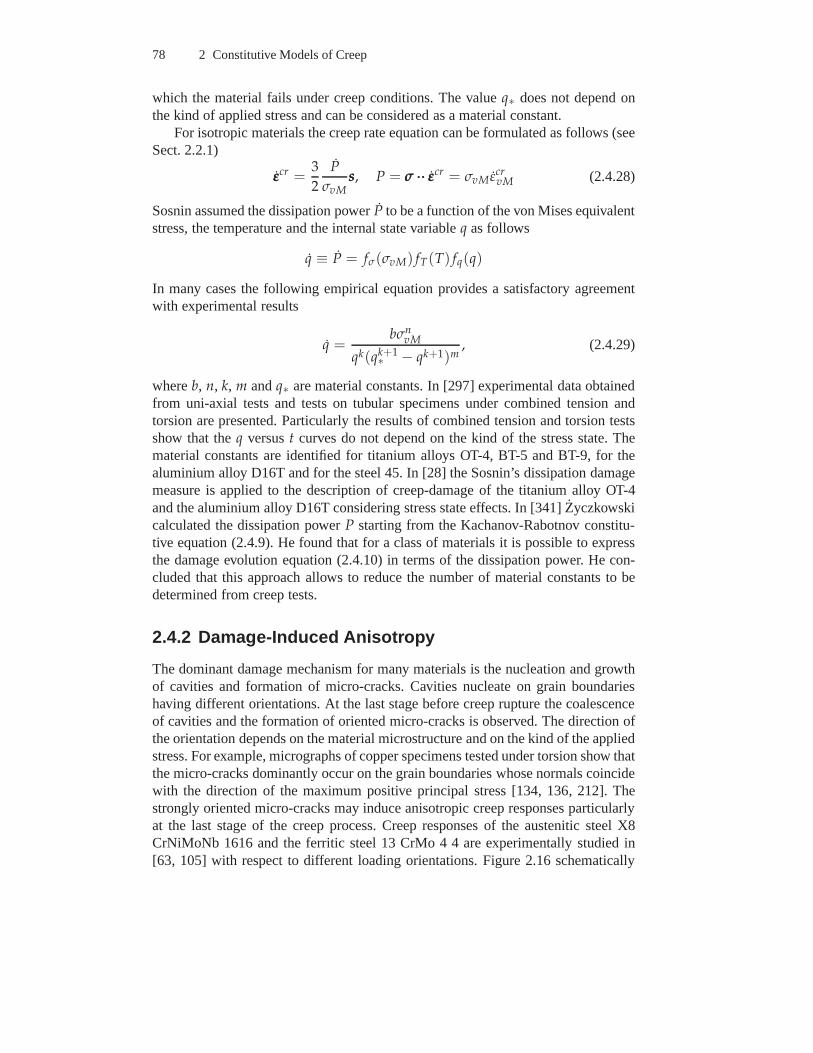
78 2 Constitutive Models of Creep
which the material fails under creep conditions. The valueq∗ does not depend onthe kind of applied stress and can be considered as a materialconstant.
For isotropic materials the creep rate equation can be formulated as follows (seeSect. 2.2.1)
εεεcr =3
2
P
σvMsss, P = σσσ ······ εεεcr = σvM εcr
vM (2.4.28)
Sosnin assumed the dissipation powerP to be a function of the von Mises equivalentstress, the temperature and the internal state variableq as follows
q ≡ P = fσ(σvM) fT(T) fq(q)
In many cases the following empirical equation provides a satisfactory agreementwith experimental results
q =bσn
vM
qk(qk+1∗ − qk+1)m
, (2.4.29)
whereb, n, k, m andq∗ are material constants. In [297] experimental data obtainedfrom uni-axial tests and tests on tubular specimens under combined tension andtorsion are presented. Particularly the results of combined tension and torsion testsshow that theq versust curves do not depend on the kind of the stress state. Thematerial constants are identified for titanium alloys OT-4,BT-5 and BT-9, for thealuminium alloy D16T and for the steel 45. In [28] the Sosnin’s dissipation damagemeasure is applied to the description of creep-damage of thetitanium alloy OT-4and the aluminium alloy D16T considering stress state effects. In [341]Zyczkowskicalculated the dissipation powerP starting from the Kachanov-Rabotnov constitu-tive equation (2.4.9). He found that for a class of materialsit is possible to expressthe damage evolution equation (2.4.10) in terms of the dissipation power. He con-cluded that this approach allows to reduce the number of material constants to bedetermined from creep tests.
2.4.2 Damage-Induced Anisotropy
The dominant damage mechanism for many materials is the nucleation and growthof cavities and formation of micro-cracks. Cavities nucleate on grain boundarieshaving different orientations. At the last stage before creep rupture the coalescenceof cavities and the formation of oriented micro-cracks is observed. The direction ofthe orientation depends on the material microstructure andon the kind of the appliedstress. For example, micrographs of copper specimens tested under torsion show thatthe micro-cracks dominantly occur on the grain boundaries whose normals coincidewith the direction of the maximum positive principal stress[134, 136, 212]. Thestrongly oriented micro-cracks may induce anisotropic creep responses particularlyat the last stage of the creep process. Creep responses of theaustenitic steel X8CrNiMoNb 1616 and the ferritic steel 13 CrMo 4 4 are experimentally studied in[63, 105] with respect to different loading orientations. Figure 2.16 schematically
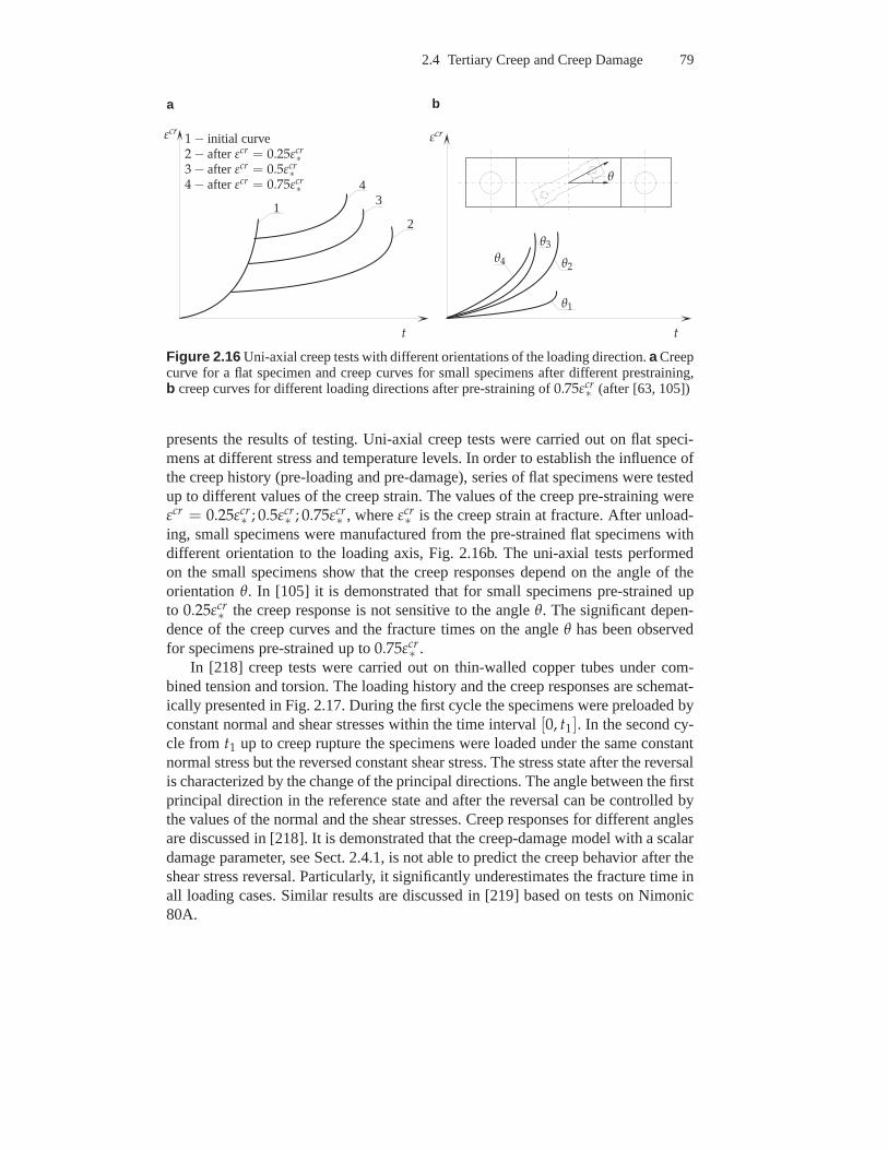
2.4 Tertiary Creep and Creep Damage 79
tt
εcrεcr
1
43
2
1 − initial curve2 − afterεcr = 0.25εcr
∗3 − afterεcr = 0.5εcr
∗4 − afterεcr = 0.75εcr
∗
θ1
θ2
θ3
θ4
θ
a b
Figure 2.16 Uni-axial creep tests with different orientations of the loading direction.a Creepcurve for a flat specimen and creep curves for small specimensafter different prestraining,b creep curves for different loading directions after pre-straining of0.75εcr
∗ (after [63, 105])
presents the results of testing. Uni-axial creep tests werecarried out on flat speci-mens at different stress and temperature levels. In order toestablish the influence ofthe creep history (pre-loading and pre-damage), series of flat specimens were testedup to different values of the creep strain. The values of the creep pre-straining wereεcr = 0.25εcr
∗ ; 0.5εcr∗ ; 0.75εcr
∗ , whereεcr∗ is the creep strain at fracture. After unload-
ing, small specimens were manufactured from the pre-strained flat specimens withdifferent orientation to the loading axis, Fig. 2.16b. The uni-axial tests performedon the small specimens show that the creep responses depend on the angle of theorientationθ. In [105] it is demonstrated that for small specimens pre-strained upto 0.25εcr
∗ the creep response is not sensitive to the angleθ. The significant depen-dence of the creep curves and the fracture times on the angleθ has been observedfor specimens pre-strained up to0.75εcr
∗ .In [218] creep tests were carried out on thin-walled copper tubes under com-
bined tension and torsion. The loading history and the creepresponses are schemat-ically presented in Fig. 2.17. During the first cycle the specimens were preloaded byconstant normal and shear stresses within the time interval[0, t1]. In the second cy-cle from t1 up to creep rupture the specimens were loaded under the same constantnormal stress but the reversed constant shear stress. The stress state after the reversalis characterized by the change of the principal directions.The angle between the firstprincipal direction in the reference state and after the reversal can be controlled bythe values of the normal and the shear stresses. Creep responses for different anglesare discussed in [218]. It is demonstrated that the creep-damage model with a scalardamage parameter, see Sect. 2.4.1, is not able to predict thecreep behavior after theshear stress reversal. Particularly, it significantly underestimates the fracture time inall loading cases. Similar results are discussed in [219] based on tests on Nimonic80A.
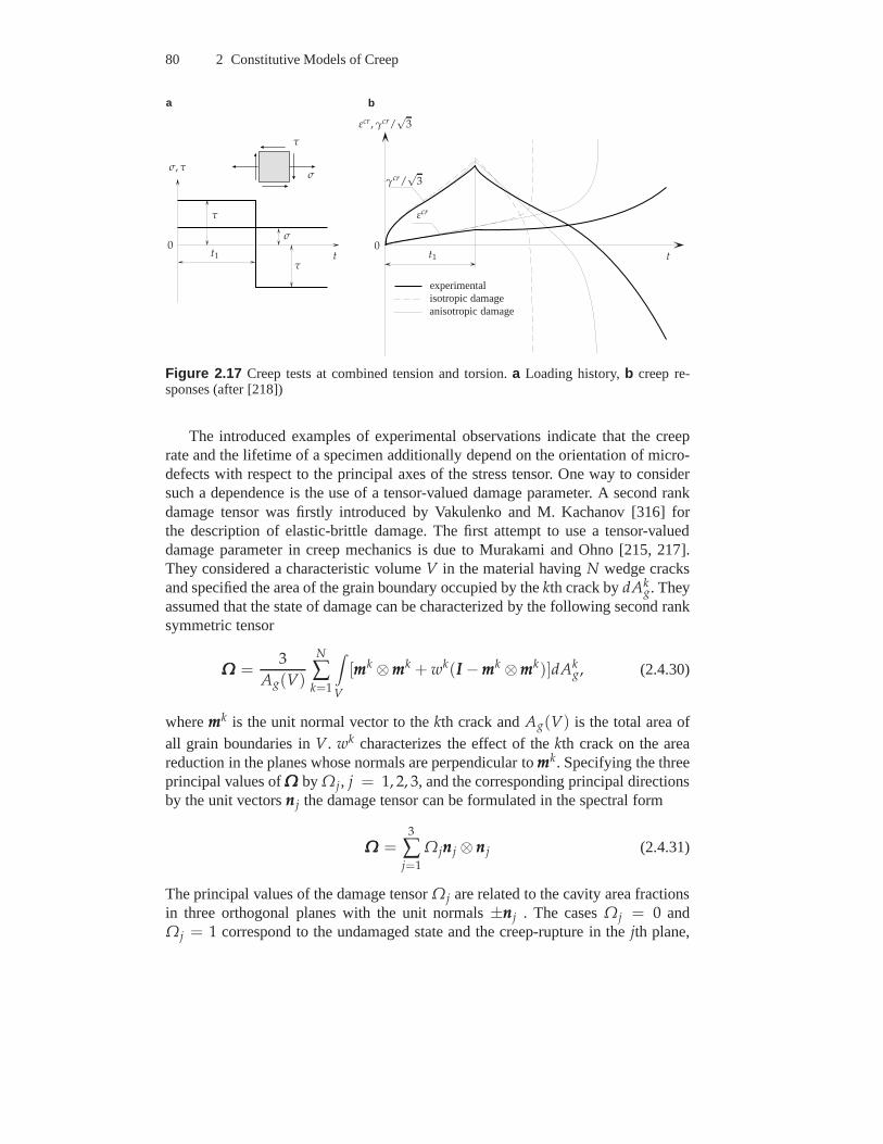
80 2 Constitutive Models of Creep
tt
εcr , γcr/√
3
σ, τ
σ
σ
τ
τ
τ
t1t100
γcr/√
3
εcr
experimentalisotropic damageanisotropic damage
a b
Figure 2.17 Creep tests at combined tension and torsion.a Loading history,b creep re-sponses (after [218])
The introduced examples of experimental observations indicate that the creeprate and the lifetime of a specimen additionally depend on the orientation of micro-defects with respect to the principal axes of the stress tensor. One way to considersuch a dependence is the use of a tensor-valued damage parameter. A second rankdamage tensor was firstly introduced by Vakulenko and M. Kachanov [316] forthe description of elastic-brittle damage. The first attempt to use a tensor-valueddamage parameter in creep mechanics is due to Murakami and Ohno [215, 217].They considered a characteristic volumeV in the material havingN wedge cracksand specified the area of the grain boundary occupied by thekth crack bydAk
g. Theyassumed that the state of damage can be characterized by the following second ranksymmetric tensor
ΩΩΩ =3
Ag(V)
N
∑k=1
∫
V
[mmmk ⊗mmmk + wk(III −mmmk ⊗mmmk)]dAkg, (2.4.30)
wheremmmk is the unit normal vector to thekth crack andAg(V) is the total area ofall grain boundaries inV. wk characterizes the effect of thekth crack on the areareduction in the planes whose normals are perpendicular tommmk. Specifying the threeprincipal values ofΩΩΩ by Ωj, j = 1, 2, 3, and the corresponding principal directionsby the unit vectorsnnnj the damage tensor can be formulated in the spectral form
ΩΩΩ =3
∑j=1
Ωjnnnj ⊗ nnnj (2.4.31)
The principal values of the damage tensorΩj are related to the cavity area fractionsin three orthogonal planes with the unit normals±nnnj . The casesΩj = 0 andΩj = 1 correspond to the undamaged state and the creep-rupture in the jth plane,
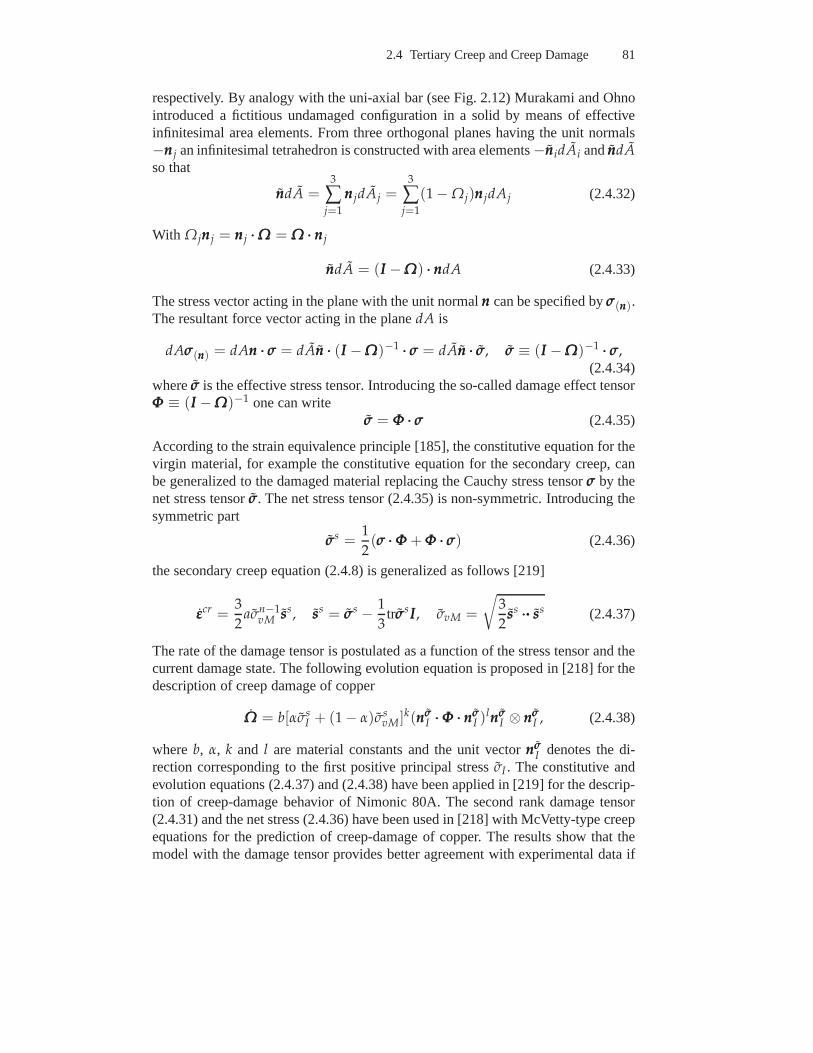
2.4 Tertiary Creep and Creep Damage 81
respectively. By analogy with the uni-axial bar (see Fig. 2.12) Murakami and Ohnointroduced a fictitious undamaged configuration in a solid bymeans of effectiveinfinitesimal area elements. From three orthogonal planes having the unit normals−nnnj an infinitesimal tetrahedron is constructed with area elements−nnnidAi andnnndAso that
nnndA =3
∑j=1
nnnjdAj =3
∑j=1
(1 − Ωj)nnnjdAj (2.4.32)
With Ωjnnnj = nnnj ···ΩΩΩ = ΩΩΩ ··· nnnj
nnndA = (III −ΩΩΩ) ··· nnndA (2.4.33)
The stress vector acting in the plane with the unit normalnnn can be specified byσσσ(nnn).The resultant force vector acting in the planedA is
dAσσσ(nnn) = dAnnn ··· σσσ = dAnnn ··· (III −ΩΩΩ)−1 ··· σσσ = dAnnn ··· σσσ, σσσ ≡ (III −ΩΩΩ)−1 ··· σσσ,(2.4.34)
whereσσσ is the effective stress tensor. Introducing the so-called damage effect tensorΦΦΦ ≡ (III −ΩΩΩ)−1 one can write
σσσ = ΦΦΦ ··· σσσ (2.4.35)
According to the strain equivalence principle [185], the constitutive equation for thevirgin material, for example the constitutive equation forthe secondary creep, canbe generalized to the damaged material replacing the Cauchystress tensorσσσ by thenet stress tensorσσσ. The net stress tensor (2.4.35) is non-symmetric. Introducing thesymmetric part
σσσs =1
2(σσσ ···ΦΦΦ + ΦΦΦ ··· σσσ) (2.4.36)
the secondary creep equation (2.4.8) is generalized as follows [219]
εεεcr =3
2aσn−1
vM ssss, ssss = σσσs − 1
3trσσσsIII, σvM =
√
3
2ssss ············ ssss (2.4.37)
The rate of the damage tensor is postulated as a function of the stress tensor and thecurrent damage state. The following evolution equation is proposed in [218] for thedescription of creep damage of copper
ΩΩΩ = b[ασsI + (1 − α)σs
vM]k(nnnσσσI ···ΦΦΦ ··· nnnσσσ
I )lnnnσσσ
I ⊗ nnnσσσI , (2.4.38)
whereb, α, k and l are material constants and the unit vectornnnσσσI denotes the di-
rection corresponding to the first positive principal stress σI . The constitutive andevolution equations (2.4.37) and (2.4.38) have been applied in [219] for the descrip-tion of creep-damage behavior of Nimonic 80A. The second rank damage tensor(2.4.31) and the net stress (2.4.36) have been used in [218] with McVetty-type creepequations for the prediction of creep-damage of copper. Theresults show that themodel with the damage tensor provides better agreement withexperimental data if
82 2 Constitutive Models of Creep
compared to the model with a scalar damage parameter, see Fig. 2.17. In [217] thefollowing damage evolution equation is utilized
ΩΩΩ = b[ασsI + βσm + (1 − α − β)σs
vM]k(tr ΦΦΦ2)l/2[
ηIII + (1 − η)nnnσσσI ⊗ nnnσσσ
I
]
,
(2.4.39)whereβ andη are material constants. This equation takes into account the influenceof the mean stress on the damage rate. Furthermore, the isotropic part of the damagetensor associated with the growth of voids is included.
To discuss the damage tensor (2.4.31) let us consider a uni-axial homogeneousstress stateσσσ = σ0mmm ⊗mmm with σ0 > 0 andmmm = const. Let us specifyΩΩΩ = 000 as theinitial condition. The evolution equation (2.4.38) takes the form
ΩΩΩ(t) = ω(t)mmm ⊗mmm, ω =bσk
0
(1 − ω)k+l, ω(0) = 0 (2.4.40)
The equation for the scalarω can be integrated as shown in Sect. 2.4.1. As a resultone can find the relation between the time to fracture and the stressσ0. Based onthis relation and experimental data one can estimate the values of material constantsb, k and l (Sect. 2.4.1). According to the introduced damage measure (2.4.31) thedamage stateΩΩΩ = ωmmm⊗mmm corresponds to the case of uniformly distributed penny-shaped cracks (circular planes) with the unit normalsmmm.
Now let us assume that the damage stateΩΩΩ = ω0mmm ⊗ mmm, 0 < ω0 < 1 isinduced as a result of the constant stressσσσ = σ0mmm ⊗ mmm exerted over a period oftime and in the next loading cycleσσσ = σ0ppp ⊗ ppp, ppp ···mmm = 0. In this case the solutionof (2.4.38) can be written down as follows
ΩΩΩ(t) = ω0mmm ⊗mmm + ω1(t)ppp ⊗ ppp, ω1 =bσk
0
(1 − ω1)k+l, ω1(0) = 0 (2.4.41)
The model predicts that in the second cycle the material behaves like a virgin un-damaged material. The corresponding time to fracture does not depend on the initialdamageω0. The rate of nucleation and growth of new voids (cracks) on the planesorthogonal toppp will not be affected by cracks formed in the first loading cycle. Fur-thermore, if a compressive stress i.e.σσσ = −σ0ppp ⊗ ppp is applied in the second cyclethe model predicts no damage accumulation.
Let us note that the evolution equations (2.4.38) and (2.4.39) can only be appliedif σI 6= 0, σI 6= σI I andσI 6= σI I I . In this case the dyadnnnσσσ
I ⊗nnnσσσI can be found from
the identity (2.4.21). For the stress statesσσσ = a0III or σσσ = appp ⊗ ppp + b(III − ppp ⊗ ppp),a < b, there is an infinite number of first principal directions. Such stress states aretypical for several structural components. For example, the stress state of the typeσσσ = appp ⊗ ppp + b(III − ppp ⊗ ppp) arises in the midpoint of a transversely loaded squareplate with all for edges to be fixed (e.g. supported or clampededges), [13]. In theloaded (top) surface of such a plateb < a < 0 while in the bottom surfaceb > a,a < 0, b > 0. Stress states of the same type arise in different rotationally symmetricproblems of structural mechanics. For analysis of such problems a modified form ofthe evolution equation (2.4.39) is required [119].
2.4 Tertiary Creep and Creep Damage 83
Various forms of creep-damage constitutive equations withsecond rank damagetensors have been utilized. In [12] the effective stress tensor
σσσ = ΦΦΦ1/2 ··· σσσ ···ΦΦΦ1/2 (2.4.42)
proposed in [91] is applied to formulate the creep-damage constitutive equation.Mechanisms of damage activation and deactivation are takeninto account. Themodel predictions are compared with experimental data of creep in copper. In[259, 260, 261, 262] a second rank damage tensor is applied for the modeling ofcreep of nickel-based single crystal super-alloys SRR 99 and CMSX-6 at760 C.The proposed constitutive equations take into account boththe initial anisotropy andthe damage induced anisotropy.
The symmetry group of a symmetric second rank tensor includes at least nine el-ements (see Sect. 2.3.2). With the second rank damage tensorand the effective stresstensors (2.4.36) or (2.4.42) only restrictive forms of orthotropic tertiary creep can beconsidered (a similar situation is discussed in Sect. 2.3.2). Therefore in many worksit is suggested to introduce higher order damage tensors. For different definitionsof damage tensors one may consult [8, 10, 55, 172, 183, 291]. Acritical reviewis given in [284]. At present, the available experimental data on creep responsesdo not allow to verify whether the orthotropic symmetry is anappropriate symme-try assumption for the modeling of anisotropic creep-damage processes. From themicro-structural point of view one may imagine rather complex three-dimensionalpatterns of voids and cracks which nucleate and propagate asthe result of multi-axialnon-proportional loadings. An attempt to predict these patterns would result in acomplex mathematical model with a large (or even infinite) number of internal vari-ables including tensors of different rank. A model to characterize different patternsof cracks may be based on the orientation distribution function, orientation averag-ing and the so-called orientation tensors. This approach iswidely used in differentbranches of physics and materials science for the statistical modeling of orientedmicro-structures. Examples include fiber suspensions [181], mixtures [112], poly-mers and polymer composites [21, 307]. The application of orientational averagingto characterize damage states under creep conditions is discussed in [212, 240, 300].
Finally let us note, that the material behavior at elevated temperature and non-proportional loading is a complex interaction of differentdeformation and damagemechanisms such as hardening, softening, creep-damage, fatigue-damage, etc. Sev-eral unified models utilize constitutive equations of creepwith kinematic and/orisotropic hardening and include damage effects by means of the effective stressconcept and the strain equivalence principle. In [158] the Malinin-Khadjinsky kine-matic hardening rule, see Sect. 2.3.2 and isotropic Kachanov-Rabotnov type damagevariable are discussed. The damage rate is additionally governed by the magnitudeof the hardening variable, so that the coupling effect of damage and strain harden-ing/softening can be taken into account. It is shown that thekinematic hardeningcoupled with isotropic damage predicts well the effect of longer life-time after thestress reversal. In [98] the Chaboche-Rousselier visco-plasticity model is modifiedto predict the coupled creep-plasticity-damage behavior.The scalar damage vari-able is introduced as a sum of the accumulated time-dependent and cycle-dependent

84 2 Constitutive Models of Creep
components. Various approaches to formulate a unified material model within theframework of continuum damage mechanics and thermodynamics of dissipativeprocesses are discussed in [85, 86, 88, 185].
The verification of a unified model with non-linear anisotropic hardeningand damage coupling requires a large number of independent tests under non-proportional loading. As a rule, accurate experimental data are rarely available.Furthermore, non-uniform stress and strain fields may be generated in a standarduni-axial specimen under non-proportional cyclic loadingconditions [189]. Theymay be the reason for the large scatter of experimental data and misleading inter-pretations.
3 Examples of Constitutive Equations forSelected Materials
In Chapter 2 we discussed theoretical approaches to the modeling of creep behav-ior. Chapter 3 deals with applications to several engineering materials. The mod-els include specific forms of the constitutive equation for the creep rate tensor andevolution equations for internal state variables. In addition, constitutive functions ofstress and temperature are specified. In order to find a set of material constants, creeptests under constant load and temperature leading to a homogeneous stress state arerequired. The majority of available experimental data is presented as creep strainversus time curves from standard uni-axial tests. Based on these curves the materialconstants are identified. It should be taken into account that experimental data mayshow a large scatter generated by testing a series of specimens removed from thesame material. The origins of scatter in creep testing are discussed in [100]. Fur-thermore, unlike small strain elasticity, the creep behavior may significantly dependon the kind of processing of specimens, e.g. the heat treatment. As a result, differ-ent data sets for the material with the same chemical composition may be found inthe literature. For example, one may compare experimental data for 9Cr1Mo (P91)ferritic steel obtained in different laboratories [1, 90, 103, 162, 242, 326].
Section 3.1 provides an overview of constitutive equationsrecently applied tocharacterize isotropic creep and long term strength of several alloys. The objectiveof Sect. 3.2 is to develop a model for anisotropic creep behavior in a weld metal pro-duced by multi-pass welding. To explain the origins of anisotropic creep, a mechan-ical model for a binary structure composed of “fine-grained”and “coarse-grained”constituents with different creep properties is introduced. The results illustrate thebasic features of the stress redistribution and damage growth in the constituents ofthe weld metal and agree qualitatively with experimental observations. The struc-tural analysis of a welded joint requires a constitutive equation of creep for theweld metal under multi-axial stress states. For this purpose we apply the approachesdeveloped in Sect 2.2.2 to model creep for initially anisotropic materials. The out-come is the a coordinate-free equation for secondary creep formulated in terms ofthe Norton-Bailey-Odqvist creep potential and three invariants of the stress tensor.The material constants are identified according to the experimental data presentedin the literature.
86 3 Examples of Constitutive Equations for Selected Materials
3.1 Models of Isotropic Creep for Several Alloys
Models of isotropic creep are discussed in Sects 2.2.1, 2.3 and 2.4.1. The creep ratetensor is assumed to be coaxial with the stress tensor (deviator) and the internalstate variables characterizing the hardening and damage processes are scalars. Theassumption of isotropic creep is usually a good approximation for many metals andalloys in the case of proportional loading. In this section we summarize the phenom-enological and mechanism-based material models and present the specific forms ofresponse functions and material constants for several alloys.
3.1.1 Type 316 Steel
The first example is type 316 stainless steel at 650 C. In [193] the following creepequations are applied
εεεcr =3
2f1(σvM)g1(ω)
sss
σvM, ω = f2
[
σωeq(σσσ)
]
g2(ω),
εεεcr|t=0 = 000, ω|t=0 = 0, 0 ≤ ω ≤ ω∗,
sss = σσσ − 1
3tr σσσIII, σvM =
√
3
2sss ······ sss
(3.1.1)
Hereεεεcr is the creep strain tensor,σσσ is the stress tensor,ω is the scalar valued dam-age parameter andσω
eq is the damage equivalent stress (see Sects 2.2.1 and 2.4.1).The response functionsf1, f2, g1, andg2 are
f1(σ) = aσn , g1(ω) = (1 − ω)−n,
f2(σ) = bσk , g2(ω) = (1 − ω)−k (3.1.2)
The material constants are presented in [193] as follows
a = 2.13 · 10−13 MPa−n/h, b = 9.1 · 10−10 MPa−k/h,n = 3.5, k = 2.8
(3.1.3)
Note, that the constantsa andb in (3.1.2) are found for the constant temperature. Inthe general case they must be replaced by functions of temperature. It is assumedthat the damage evolution is controlled by the maximum tensile stress. In this casethe damage equivalent stress takes the form
σωeq(σσσ) =
σI + |σI |2
,
whereσI is the first principal stress. The elastic material behavioris characterizedby the following values of the Young’s modulusE and the Poisson’s ratioν
E = 1.44 · 105 MPa, ν = 0.314 (3.1.4)
Let us note that the response functions and material constants in Eqs (3.1.1) canbe found in the literature for numerous metals and alloys. Examples are presentedin the monographs [77, 185, 202, 250, 255, 265, 291].
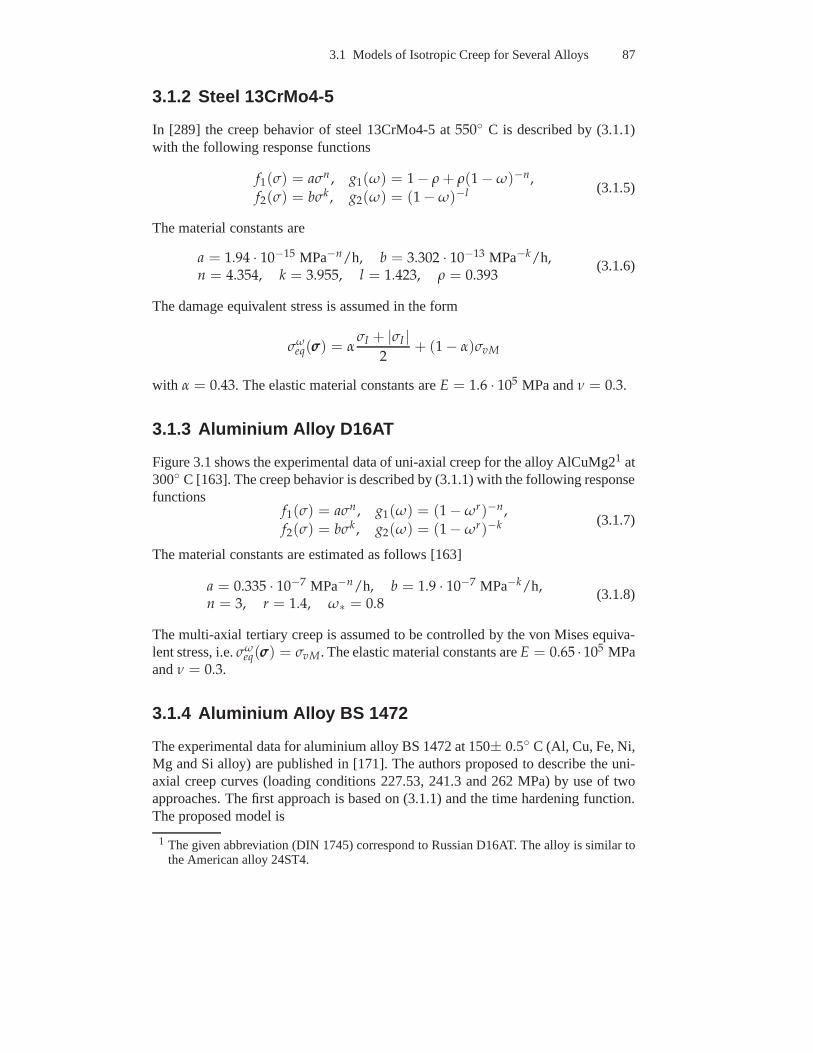
3.1 Models of Isotropic Creep for Several Alloys 87
3.1.2 Steel 13CrMo4-5
In [289] the creep behavior of steel 13CrMo4-5 at550 C is described by (3.1.1)with the following response functions
f1(σ) = aσn , g1(ω) = 1 − ρ + ρ(1 − ω)−n,
f2(σ) = bσk , g2(ω) = (1 − ω)−l (3.1.5)
The material constants are
a = 1.94 · 10−15 MPa−n/h, b = 3.302 · 10−13 MPa−k/h,n = 4.354, k = 3.955, l = 1.423, ρ = 0.393
(3.1.6)
The damage equivalent stress is assumed in the form
σωeq(σσσ) = α
σI + |σI |2
+ (1 − α)σvM
with α = 0.43. The elastic material constants areE = 1.6 · 105 MPa andν = 0.3.
3.1.3 Aluminium Alloy D16AT
Figure 3.1 shows the experimental data of uni-axial creep for the alloy AlCuMg21 at300 C [163]. The creep behavior is described by (3.1.1) with the following responsefunctions
f1(σ) = aσn , g1(ω) = (1 − ωr)−n,
f2(σ) = bσk , g2(ω) = (1 − ωr)−k (3.1.7)
The material constants are estimated as follows [163]
a = 0.335 · 10−7 MPa−n/h, b = 1.9 · 10−7 MPa−k/h,n = 3, r = 1.4, ω∗ = 0.8
(3.1.8)
The multi-axial tertiary creep is assumed to be controlled by the von Mises equiva-lent stress, i.e.σω
eq(σσσ) = σvM. The elastic material constants areE = 0.65 · 105 MPaandν = 0.3.
3.1.4 Aluminium Alloy BS 1472
The experimental data for aluminium alloy BS 1472 at 150± 0.5 C (Al, Cu, Fe, Ni,Mg and Si alloy) are published in [171]. The authors proposedto describe the uni-axial creep curves (loading conditions 227.53, 241.3 and 262 MPa) by use of twoapproaches. The first approach is based on (3.1.1) and the time hardening function.The proposed model is
1 The given abbreviation (DIN 1745) correspond to Russian D16AT. The alloy is similar tothe American alloy 24ST4.
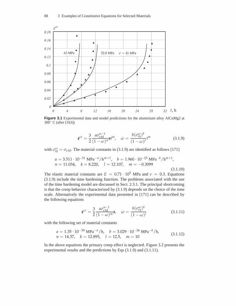
88 3 Examples of Constitutive Equations for Selected Materials
0 4 8 1 2 1 6 2 0 2 4 2 8 3 20
0 . 0 2
0 . 0 4
0 . 0 6
0 . 0 8
0 . 1
0 . 1 2
0 . 1 4
0 . 1 6
0 . 1 8
t, h
εcr
σ = 41 MPa52.8 MPa63 MPa
Figure 3.1 Experimental data and model predictions for the aluminium alloy AlCuMg2 at300 C (after [163])
εεεcr =3
2
aσn−1vM
(1 − ω)nssstm, ω =
b(σωeq)
k
(1 − ω)ltm (3.1.9)
with σωeq = σvM. The material constants in (3.1.9) are identified as follows[171]
a = 3.511 · 10−31 MPa−n/hm+1, b = 1.960 · 10−23 MPa−k/hm+1,n = 11.034, k = 8.220, l = 12.107, m = −0.3099
(3.1.10)The elastic material constants areE = 0.71 · 105 MPa andν = 0.3. Equations(3.1.9) include the time hardening function. The problems associated with the useof the time hardening model are discussed in Sect. 2.3.1. Theprincipal shortcomingis that the creep behavior characterized by (3.1.9) dependson the choice of the timescale. Alternatively the experimental data presented in [171] can be described bythe following equations
εεεcr =3
2
aσn−1vM
(1 − ω)msss, ω =
b(σωeq)
k
(1 − ω)l(3.1.11)
with the following set of material constants
a = 1.35 · 10−39 MPa−n/h, b = 3.029 · 10−36 MPa−k/h,n = 14.37, k = 12.895, l = 12.5, m = 10
(3.1.12)
In the above equations the primary creep effect is neglected. Figure 3.2 presents theexperimental results and the predictions by Eqs (3.1.9) and(3.1.11).
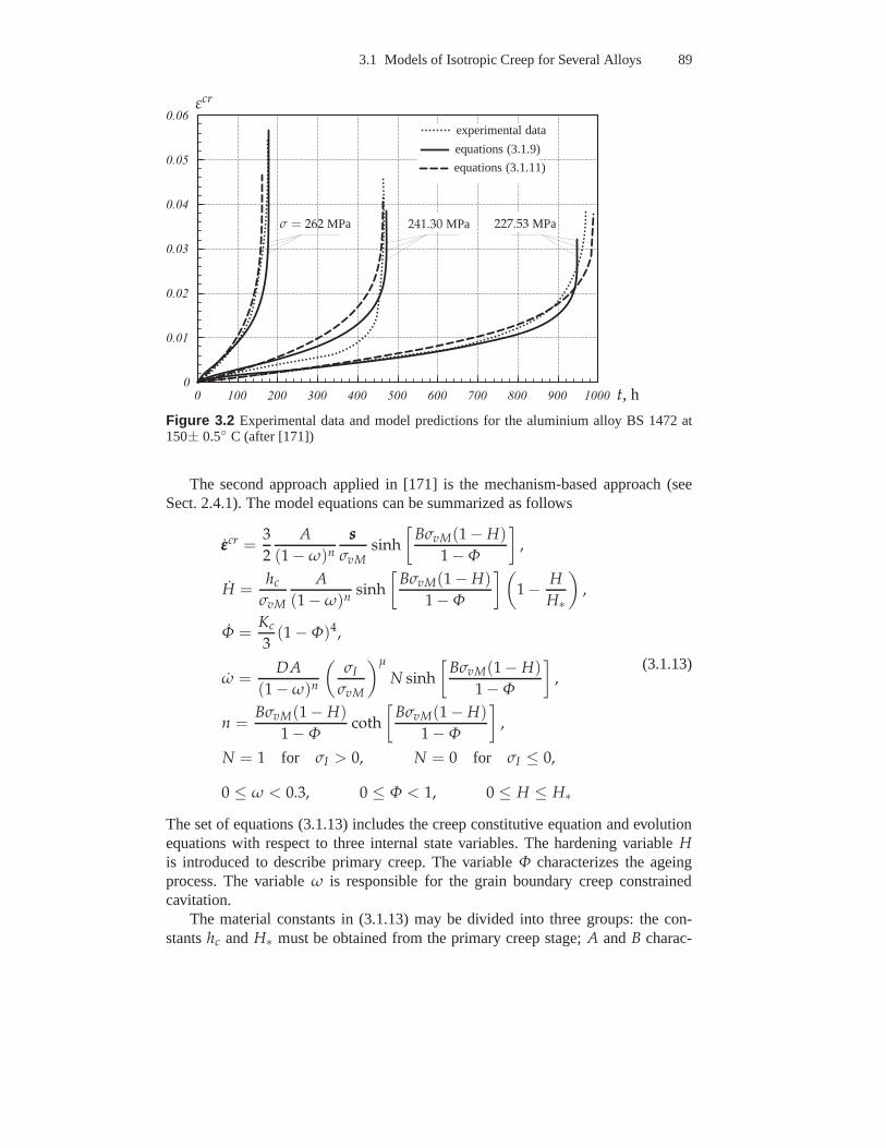
3.1 Models of Isotropic Creep for Several Alloys 89
0 1 0 0 2 0 0 3 0 0 4 0 0 5 0 0 6 0 0 7 0 0 8 0 0 9 0 0 1 0 0 00
0 . 0 1
0 . 0 2
0 . 0 3
0 . 0 4
0 . 0 5
0 . 0 6
t, h
εcr
σ = 262 MPa 241.30 MPa 227.53 MPa
experimental data
equations (3.1.9)
equations (3.1.11)
Figure 3.2 Experimental data and model predictions for the aluminium alloy BS 1472 at150± 0.5 C (after [171])
The second approach applied in [171] is the mechanism-basedapproach (seeSect. 2.4.1). The model equations can be summarized as follows
εεεcr =3
2
A
(1 − ω)n
sss
σvMsinh
[
BσvM(1 − H)
1 − Φ
]
,
H =hc
σvM
A
(1 − ω)nsinh
[
BσvM(1 − H)
1 − Φ
] (
1 − H
H∗
)
,
Φ =Kc
3(1 − Φ)4,
ω =DA
(1 − ω)n
(
σI
σvM
)µ
N sinh
[
BσvM(1 − H)
1 − Φ
]
,
n =BσvM(1 − H)
1 − Φcoth
[
BσvM(1 − H)
1 − Φ
]
,
N = 1 for σI > 0, N = 0 for σI ≤ 0,
0 ≤ ω < 0.3, 0 ≤ Φ < 1, 0 ≤ H ≤ H∗
(3.1.13)
The set of equations (3.1.13) includes the creep constitutive equation and evolutionequations with respect to three internal state variables. The hardening variableHis introduced to describe primary creep. The variableΦ characterizes the ageingprocess. The variableω is responsible for the grain boundary creep constrainedcavitation.
The material constants in (3.1.13) may be divided into threegroups: the con-stantshc andH∗ must be obtained from the primary creep stage;A andB charac-
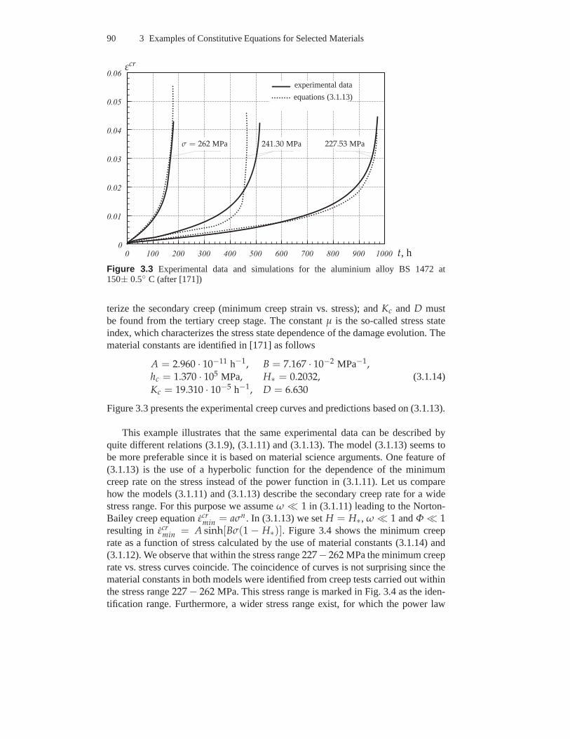
90 3 Examples of Constitutive Equations for Selected Materials
0 1 0 0 2 0 0 3 0 0 4 0 0 5 0 0 6 0 0 7 0 0 8 0 0 9 0 0 1 0 0 00
0 . 0 1
0 . 0 2
0 . 0 3
0 . 0 4
0 . 0 5
0 . 0 6
t, h
εcr
σ = 262 MPa 241.30 MPa 227.53 MPa
experimental data
equations (3.1.13)
Figure 3.3 Experimental data and simulations for the aluminium alloy BS 1472 at150± 0.5 C (after [171])
terize the secondary creep (minimum creep strain vs. stress); andKc and D mustbe found from the tertiary creep stage. The constantµ is the so-called stress stateindex, which characterizes the stress state dependence of the damage evolution. Thematerial constants are identified in [171] as follows
A = 2.960 · 10−11 h−1, B = 7.167 · 10−2 MPa−1,hc = 1.370 · 105 MPa, H∗ = 0.2032,
Kc = 19.310 · 10−5 h−1, D = 6.630
(3.1.14)
Figure 3.3 presents the experimental creep curves and predictions based on (3.1.13).
This example illustrates that the same experimental data can be described byquite different relations (3.1.9), (3.1.11) and (3.1.13).The model (3.1.13) seems tobe more preferable since it is based on material science arguments. One feature of(3.1.13) is the use of a hyperbolic function for the dependence of the minimumcreep rate on the stress instead of the power function in (3.1.11). Let us comparehow the models (3.1.11) and (3.1.13) describe the secondarycreep rate for a widestress range. For this purpose we assumeω ≪ 1 in (3.1.11) leading to the Norton-Bailey creep equationεcr
min = aσn . In (3.1.13) we setH = H∗, ω ≪ 1 andΦ ≪ 1resulting in εcr
min = A sinh[Bσ(1 − H∗)]. Figure 3.4 shows the minimum creeprate as a function of stress calculated by the use of materialconstants (3.1.14) and(3.1.12). We observe that within the stress range227− 262 MPa the minimum creeprate vs. stress curves coincide. The coincidence of curves is not surprising since thematerial constants in both models were identified from creeptests carried out withinthe stress range227 − 262 MPa. This stress range is marked in Fig. 3.4 as the iden-tification range. Furthermore, a wider stress range exist, for which the power law
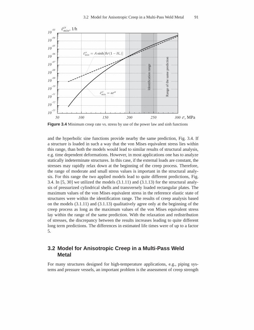
3.2 Model for Anisotropic Creep in a Multi-Pass Weld Metal 91
5 0 1 0 0 1 5 0 2 0 0 2 5 0 3 0 01 0
- 1 3
1 0- 1 2
1 0- 1 1
1 0- 1 0
1 0- 0 9
1 0- 0 8
1 0- 0 7
1 0- 0 6
1 0- 0 5
1 0- 0 4
1 0- 0 3
σ, MPa
εcrmin, 1/h
Iden
tifica
tion
rang
e
Ran
geof
the
sam
epr
edic
tionεcr
min = A sinh[Bσ(1 − H∗)]
εcrmin = aσn
Figure 3.4 Minimum creep rate vs. stress by use of the power law and sinh functions
and the hyperbolic sine functions provide nearby the same prediction, Fig. 3.4. Ifa structure is loaded in such a way that the von Mises equivalent stress lies withinthis range, than both the models would lead to similar results of structural analysis,e.g. time dependent deformations. However, in most applications one has to analyzestatically indeterminate structures. In this case, if the external loads are constant, thestresses may rapidly relax down at the beginning of the creepprocess. Therefore,the range of moderate and small stress values is important inthe structural analy-sis. For this range the two applied models lead to quite different predictions, Fig.3.4. In [5, 30] we utilized the models (3.1.11) and (3.1.13) for the structural analy-sis of pressurized cylindrical shells and transversely loaded rectangular plates. Themaximum values of the von Mises equivalent stress in the reference elastic state ofstructures were within the identification range. The results of creep analysis basedon the models (3.1.11) and (3.1.13) qualitatively agree only at the beginning of thecreep process as long as the maximum values of the von Mises equivalent stresslay within the range of the same prediction. With the relaxation and redistributionof stresses, the discrepancy between the results increasesleading to quite differentlong term predictions. The differences in estimated life times were of up to a factor5.
3.2 Model for Anisotropic Creep in a Multi-Pass WeldMetal
For many structures designed for high-temperature applications, e.g., piping sys-tems and pressure vessels, an important problem is the assessment of creep strength
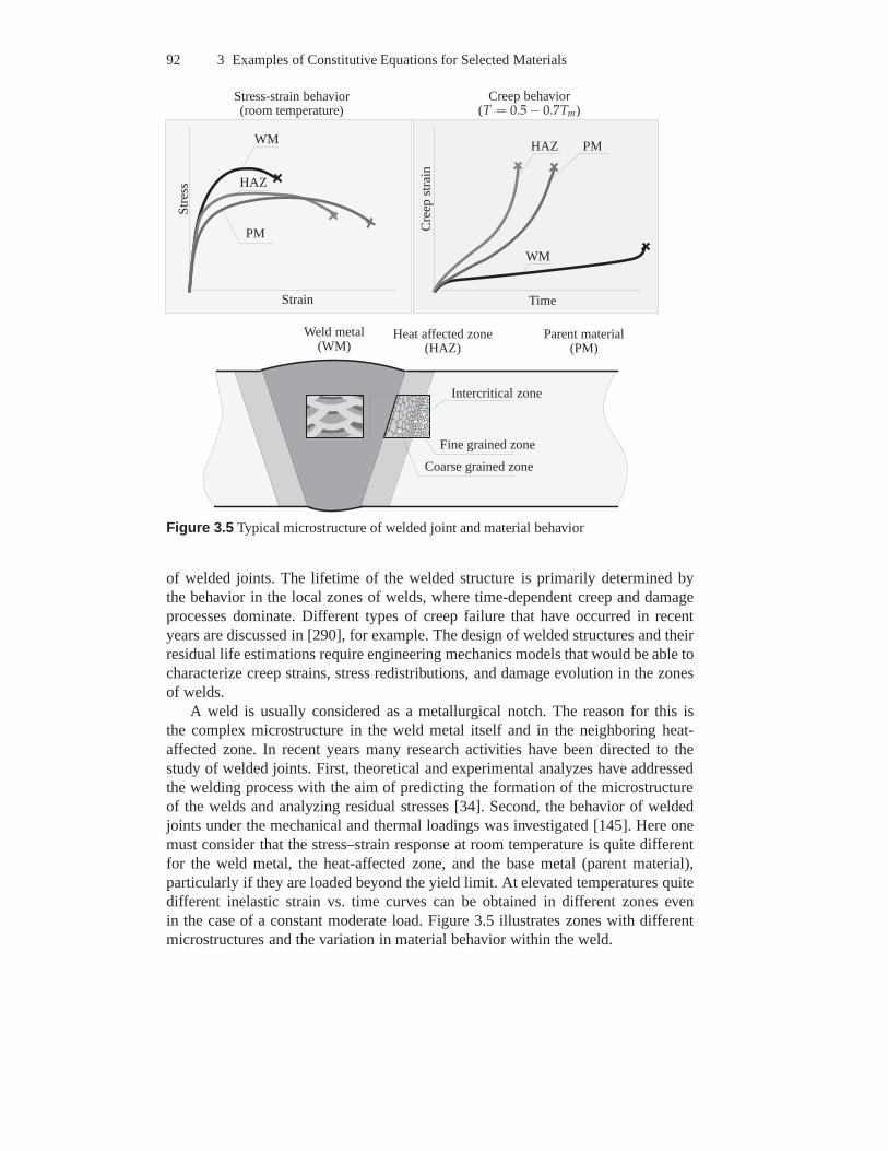
92 3 Examples of Constitutive Equations for Selected Materials
Time
Cre
epst
rain
Strain
Str
ess
Stress-strain behavior(room temperature)
Creep behavior(T = 0.5 − 0.7Tm)
Weld metal(WM)
Heat affected zone(HAZ)
Parent material(PM)
WM
WM HAZ
HAZ
PM
PM
Coarse grained zone
Fine grained zone
Intercritical zone
Figure 3.5 Typical microstructure of welded joint and material behavior
of welded joints. The lifetime of the welded structure is primarily determined bythe behavior in the local zones of welds, where time-dependent creep and damageprocesses dominate. Different types of creep failure that have occurred in recentyears are discussed in [290], for example. The design of welded structures and theirresidual life estimations require engineering mechanics models that would be able tocharacterize creep strains, stress redistributions, and damage evolution in the zonesof welds.
A weld is usually considered as a metallurgical notch. The reason for this isthe complex microstructure in the weld metal itself and in the neighboring heat-affected zone. In recent years many research activities have been directed to thestudy of welded joints. First, theoretical and experimental analyzes have addressedthe welding process with the aim of predicting the formationof the microstructureof the welds and analyzing residual stresses [34]. Second, the behavior of weldedjoints under the mechanical and thermal loadings was investigated [145]. Here onemust consider that the stress–strain response at room temperature is quite differentfor the weld metal, the heat-affected zone, and the base metal (parent material),particularly if they are loaded beyond the yield limit. At elevated temperatures quitedifferent inelastic strain vs. time curves can be obtained in different zones evenin the case of a constant moderate load. Figure 3.5 illustrates zones with differentmicrostructures and the variation in material behavior within the weld.
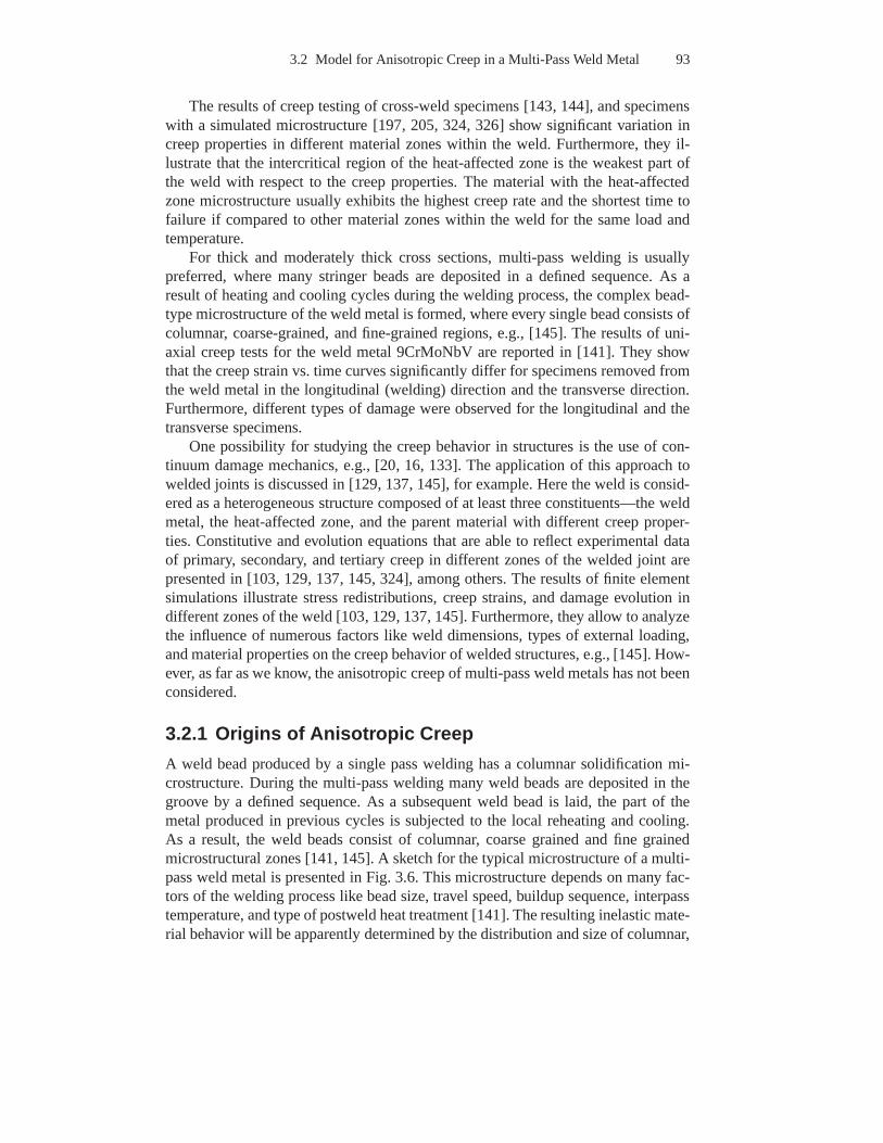
3.2 Model for Anisotropic Creep in a Multi-Pass Weld Metal 93
The results of creep testing of cross-weld specimens [143, 144], and specimenswith a simulated microstructure [197, 205, 324, 326] show significant variation increep properties in different material zones within the weld. Furthermore, they il-lustrate that the intercritical region of the heat-affected zone is the weakest part ofthe weld with respect to the creep properties. The material with the heat-affectedzone microstructure usually exhibits the highest creep rate and the shortest time tofailure if compared to other material zones within the weld for the same load andtemperature.
For thick and moderately thick cross sections, multi-pass welding is usuallypreferred, where many stringer beads are deposited in a defined sequence. As aresult of heating and cooling cycles during the welding process, the complex bead-type microstructure of the weld metal is formed, where everysingle bead consists ofcolumnar, coarse-grained, and fine-grained regions, e.g.,[145]. The results of uni-axial creep tests for the weld metal 9CrMoNbV are reported in[141]. They showthat the creep strain vs. time curves significantly differ for specimens removed fromthe weld metal in the longitudinal (welding) direction and the transverse direction.Furthermore, different types of damage were observed for the longitudinal and thetransverse specimens.
One possibility for studying the creep behavior in structures is the use of con-tinuum damage mechanics, e.g., [20, 16, 133]. The application of this approach towelded joints is discussed in [129, 137, 145], for example. Here the weld is consid-ered as a heterogeneous structure composed of at least threeconstituents—the weldmetal, the heat-affected zone, and the parent material withdifferent creep proper-ties. Constitutive and evolution equations that are able toreflect experimental dataof primary, secondary, and tertiary creep in different zones of the welded joint arepresented in [103, 129, 137, 145, 324], among others. The results of finite elementsimulations illustrate stress redistributions, creep strains, and damage evolution indifferent zones of the weld [103, 129, 137, 145]. Furthermore, they allow to analyzethe influence of numerous factors like weld dimensions, types of external loading,and material properties on the creep behavior of welded structures, e.g., [145]. How-ever, as far as we know, the anisotropic creep of multi-pass weld metals has not beenconsidered.
3.2.1 Origins of Anisotropic Creep
A weld bead produced by a single pass welding has a columnar solidification mi-crostructure. During the multi-pass welding many weld beads are deposited in thegroove by a defined sequence. As a subsequent weld bead is laid, the part of themetal produced in previous cycles is subjected to the local reheating and cooling.As a result, the weld beads consist of columnar, coarse grained and fine grainedmicrostructural zones [141, 145]. A sketch for the typical microstructure of a multi-pass weld metal is presented in Fig. 3.6. This microstructure depends on many fac-tors of the welding process like bead size, travel speed, buildup sequence, interpasstemperature, and type of postweld heat treatment [141]. Theresulting inelastic mate-rial behavior will be apparently determined by the distribution and size of columnar,
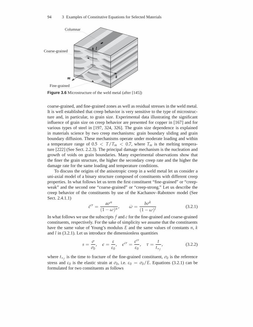
94 3 Examples of Constitutive Equations for Selected Materials
Columnar
Coarse-grained
Fine-grained
mmm kkk
lll
Figure 3.6 Microstructure of the weld metal (after [145])
coarse-grained, and fine-grained zones as well as residual stresses in the weld metal.It is well established that creep behavior is very sensitiveto the type of microstruc-ture and, in particular, to grain size. Experimental data illustrating the significantinfluence of grain size on creep behavior are presented for copper in [167] and forvarious types of steel in [197, 324, 326]. The grain size dependence is explainedin materials science by two creep mechanisms: grain boundary sliding and grainboundary diffusion. These mechanisms operate under moderate loading and withina temperature range of0.5 < T/Tm < 0.7, whereTm is the melting tempera-ture [222] (See Sect. 2.2.3). The principal damage mechanism is the nucleation andgrowth of voids on grain boundaries. Many experimental observations show thatthe finer the grain structure, the higher the secondary creeprate and the higher thedamage rate for the same loading and temperature conditions.
To discuss the origins of the anisotropic creep in a weld metal let us consider auni-axial model of a binary structure composed of constituents with different creepproperties. In what follows let us term the first constituent“fine-grained” or “creep-weak” and the second one “coarse-grained” or “creep-strong.” Let us describe thecreep behavior of the constituents by use of the Kachanov–Rabotnov model (SeeSect. 2.4.1.1)
εcr =aσn
(1 − ω)n, ω =
bσk
(1 − ω)l(3.2.1)
In what follows we use the subscriptsf andc for the fine-grained and coarse-grainedconstituents, respectively. For the sake of simplicity we assume that the constituentshave the same value of Young’s modulusE and the same values of constantsn, kandl in (3.2.1). Let us introduce the dimensionless quantities
s =σ
σ0, ǫ =
ε
ε0, ǫcr =
εcr
ε0, τ =
t
t∗ f
, (3.2.2)
wheret∗ fis the time to fracture of the fine-grained constituent,σ0 is the reference
stress andε0 is the elastic strain atσ0, i.e. ε0 = σ0/E. Equations (3.2.1) can beformulated for two constituents as follows
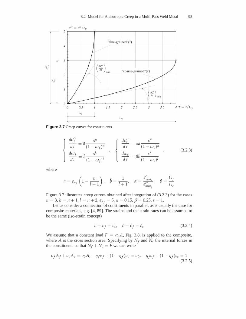
3.2 Model for Anisotropic Creep in a Multi-Pass Weld Metal 95
0 0 . 5 1 1 . 5 2 2 . 5 3 3 . 5 40
1
2
3
4
5
τ = t/t∗ f
ǫcr = εcr/ε0
”fine-grained”(f)
”coarse-grained”(c)
(
dǫcrf
dτ
)
min
(
dǫcrc
dτ
)
min
τ∗c
τ∗ f
ǫcr ∗ c
ǫcr ∗ f
Figure 3.7 Creep curves for constituents
dǫcrf
dτ= a
sn
(1 − ω f )n
dω f
dτ= b
sk
(1 − ω f )l
,
dǫcrc
dτ= αa
sn
(1 − ωc)n
dωc
dτ= βb
sk
(1 − ωc)l
, (3.2.3)
where
a = ǫ∗ f
(
1 − n
l + 1
)
, b =1
l + 1, α =
εcrminc
εcrmin f
, β =t∗ f
t∗c
Figure 3.7 illustrates creep curves obtained after integration of (3.2.3) for the casesn = 3, k = n + 1, l = n + 2, ǫ∗ f
= 5, α = 0.15, β = 0.25, s = 1.Let us consider a connection of constituents in parallel, asis usually the case for
composite materials, e.g. [4, 89]. The strains and the strain rates can be assumed tobe the same (iso-strain concept)
ε = ε f = εc, ε = ε f = εc (3.2.4)
We assume that a constant loadF = σ0 A, Fig. 3.8, is applied to the composite,whereA is the cross section area. Specifying byN f and Nc the internal forces inthe constituents so thatN f + Nc = F we can write
σf A f + σc Ac = σ0 A, η f σf + (1 − η f )σc = σ0, η f s f + (1 − η f )sc = 1(3.2.5)
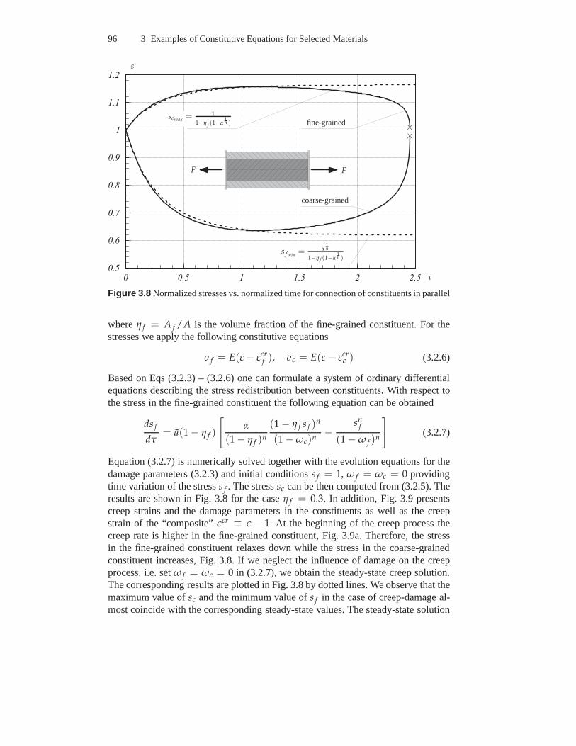
96 3 Examples of Constitutive Equations for Selected Materials
0 0 . 5 1 1 . 5 2 2 . 50 . 5
0 . 6
0 . 7
0 . 8
0 . 9
1
1 . 1
1 . 2
τ
s
fine-grained
coarse-grained
scmax = 1
1−η f (1−α1n )
s fmin= α
1n
1−η f (1−α1n )
FF
Figure 3.8 Normalized stresses vs. normalized time for connection of constituents in parallel
whereη f = A f /A is the volume fraction of the fine-grained constituent. For thestresses we apply the following constitutive equations
σf = E(ε − εcrf ), σc = E(ε − εcr
c ) (3.2.6)
Based on Eqs (3.2.3) – (3.2.6) one can formulate a system of ordinary differentialequations describing the stress redistribution between constituents. With respect tothe stress in the fine-grained constituent the following equation can be obtained
ds f
dτ= a(1 − η f )
[
α
(1 − η f )n
(1 − η f s f )n
(1 − ωc)n−
snf
(1 − ω f )n
]
(3.2.7)
Equation (3.2.7) is numerically solved together with the evolution equations for thedamage parameters (3.2.3) and initial conditionss f = 1, ω f = ωc = 0 providingtime variation of the stresss f . The stresssc can be then computed from (3.2.5). Theresults are shown in Fig. 3.8 for the caseη f = 0.3. In addition, Fig. 3.9 presentscreep strains and the damage parameters in the constituentsas well as the creepstrain of the “composite”ǫcr ≡ ǫ − 1. At the beginning of the creep process thecreep rate is higher in the fine-grained constituent, Fig. 3.9a. Therefore, the stressin the fine-grained constituent relaxes down while the stress in the coarse-grainedconstituent increases, Fig. 3.8. If we neglect the influenceof damage on the creepprocess, i.e. setω f = ωc = 0 in (3.2.7), we obtain the steady-state creep solution.The corresponding results are plotted in Fig. 3.8 by dotted lines. We observe that themaximum value ofsc and the minimum value ofs f in the case of creep-damage al-most coincide with the corresponding steady-state values.The steady-state solution
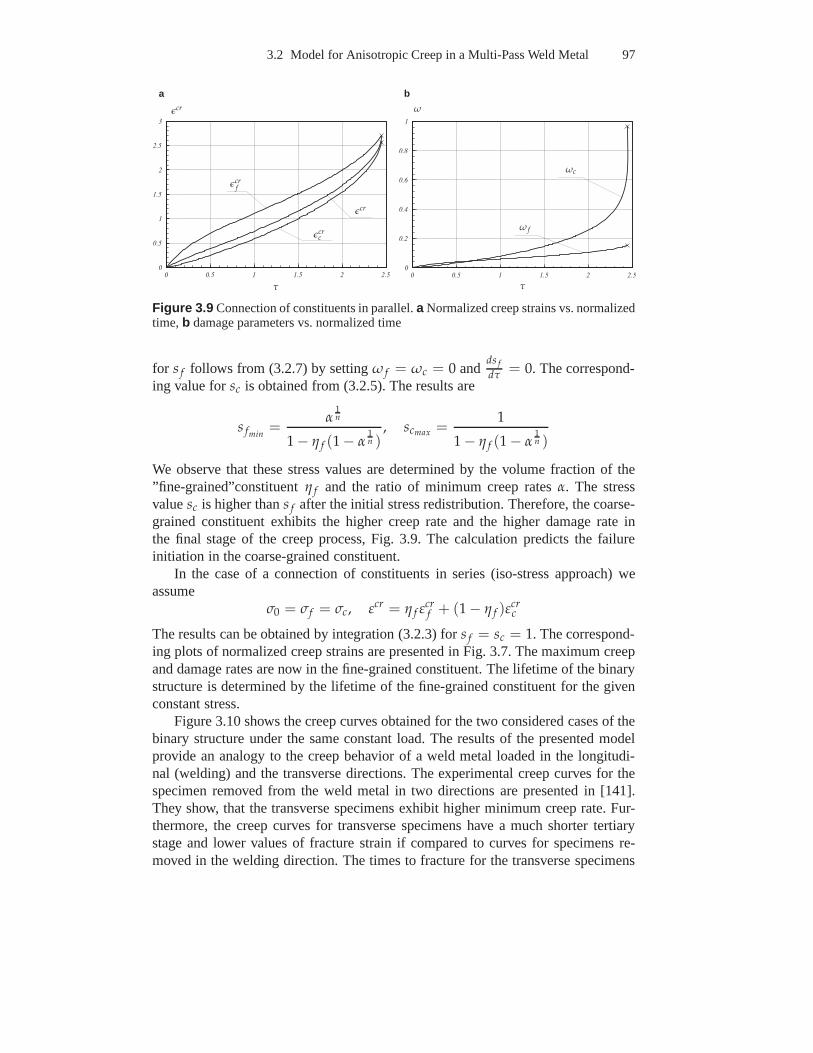
3.2 Model for Anisotropic Creep in a Multi-Pass Weld Metal 97
0 0 . 5 1 1 . 5 2 2 . 50
0 . 5
1
1 . 5
2
2 . 5
3
0 0 . 5 1 1 . 5 2 2 . 50
0 . 2
0 . 4
0 . 6
0 . 8
1
ττ
ǫcr ω
ǫcrc
ǫcr
ǫcrf
ω f
ωc
a b
Figure 3.9 Connection of constituents in parallel.a Normalized creep strains vs. normalizedtime,b damage parameters vs. normalized time
for s f follows from (3.2.7) by settingω f = ωc = 0 andds f
dτ = 0. The correspond-ing value forsc is obtained from (3.2.5). The results are
s fmin=
α1n
1 − η f (1 − α1n )
, scmax =1
1 − η f (1 − α1n )
We observe that these stress values are determined by the volume fraction of the”fine-grained”constituentη f and the ratio of minimum creep ratesα. The stressvaluesc is higher thans f after the initial stress redistribution. Therefore, the coarse-grained constituent exhibits the higher creep rate and the higher damage rate inthe final stage of the creep process, Fig. 3.9. The calculation predicts the failureinitiation in the coarse-grained constituent.
In the case of a connection of constituents in series (iso-stress approach) weassume
σ0 = σf = σc, εcr = η f εcrf + (1 − η f )εcr
c
The results can be obtained by integration (3.2.3) fors f = sc = 1. The correspond-ing plots of normalized creep strains are presented in Fig. 3.7. The maximum creepand damage rates are now in the fine-grained constituent. Thelifetime of the binarystructure is determined by the lifetime of the fine-grained constituent for the givenconstant stress.
Figure 3.10 shows the creep curves obtained for the two considered cases of thebinary structure under the same constant load. The results of the presented modelprovide an analogy to the creep behavior of a weld metal loaded in the longitudi-nal (welding) and the transverse directions. The experimental creep curves for thespecimen removed from the weld metal in two directions are presented in [141].They show, that the transverse specimens exhibit higher minimum creep rate. Fur-thermore, the creep curves for transverse specimens have a much shorter tertiarystage and lower values of fracture strain if compared to curves for specimens re-moved in the welding direction. The times to fracture for thetransverse specimens
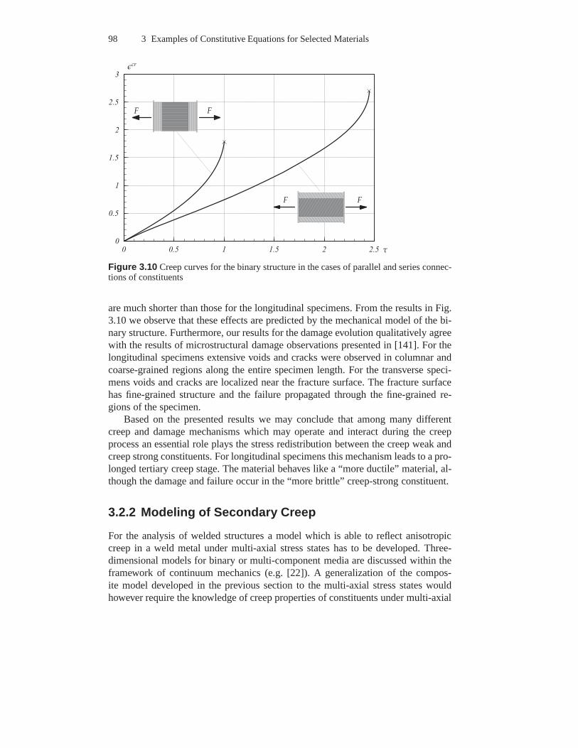
98 3 Examples of Constitutive Equations for Selected Materials
0 0 . 5 1 1 . 5 2 2 . 50
0 . 5
1
1 . 5
2
2 . 5
3
τ
ǫcr
FF
F F
Figure 3.10 Creep curves for the binary structure in the cases of parallel and series connec-tions of constituents
are much shorter than those for the longitudinal specimens.From the results in Fig.3.10 we observe that these effects are predicted by the mechanical model of the bi-nary structure. Furthermore, our results for the damage evolution qualitatively agreewith the results of microstructural damage observations presented in [141]. For thelongitudinal specimens extensive voids and cracks were observed in columnar andcoarse-grained regions along the entire specimen length. For the transverse speci-mens voids and cracks are localized near the fracture surface. The fracture surfacehas fine-grained structure and the failure propagated through the fine-grained re-gions of the specimen.
Based on the presented results we may conclude that among many differentcreep and damage mechanisms which may operate and interact during the creepprocess an essential role plays the stress redistribution between the creep weak andcreep strong constituents. For longitudinal specimens this mechanism leads to a pro-longed tertiary creep stage. The material behaves like a “more ductile” material, al-though the damage and failure occur in the “more brittle” creep-strong constituent.
3.2.2 Modeling of Secondary Creep
For the analysis of welded structures a model which is able toreflect anisotropiccreep in a weld metal under multi-axial stress states has to be developed. Three-dimensional models for binary or multi-component media arediscussed within theframework of continuum mechanics (e.g. [22]). A generalization of the compos-ite model developed in the previous section to the multi-axial stress states wouldhowever require the knowledge of creep properties of constituents under multi-axial
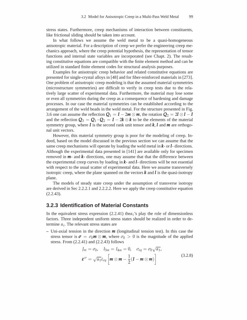
3.2 Model for Anisotropic Creep in a Multi-Pass Weld Metal 99
stress states. Furthermore, creep mechanisms of interaction between constituents,like frictional sliding should be taken into account.
In what follows we assume the weld metal to be a quasi-homogeneousanisotropic material. For a description of creep we prefer the engineering creep me-chanics approach, where the creep potential hypothesis, the representation of tensorfunctions and internal state variables are incorporated (see Chapt. 2). The result-ing constitutive equations are compatible with the finite element method and can beutilized in standard finite element codes for structural analysis purposes.
Examples for anisotropic creep behavior and related constitutive equations arepresented for single-crystal alloys in [48] and for fiber-reinforced materials in [273].One problem of anisotropic creep modeling is that the assumed material symmetries(microstructure symmetries) are difficult to verify in creep tests due to the rela-tively large scatter of experimental data. Furthermore, the material may lose someor even all symmetries during the creep as a consequence of hardening and damageprocesses. In our case the material symmetries can be established according to thearrangement of the weld beads in the weld metal. For the structure presented in Fig.3.6 one can assume the reflectionQQQ1 = III − 2mmm ⊗mmm, the rotationQQQ2 = 2lll ⊗ lll − IIIand the reflectionQQQ3 = QQQ1 ··· QQQ2 = III − 2kkk ⊗ kkk to be the elements of the materialsymmetry group, whereIII is the second rank unit tensor andkkk, lll andmmm are orthogo-nal unit vectors.
However, this material symmetry group is poor for the modeling of creep. In-deed, based on the model discussed in the previous section wecan assume that thesame creep mechanisms will operate by loading the weld metalin kkk- or lll- directions.Although the experimental data presented in [141] are available only for specimenremoved inmmm- andkkk- directions, one may assume that that the difference betweenthe experimental creep curves by loading inkkk- andlll- directions will be not essentialwith respect to the usual scatter of experimental data. Herewe assume transverselyisotropic creep, where the plane spanned on the vectorskkk andlll is the quasi-isotropyplane.
The models of steady state creep under the assumption of transverse isotropyare derived in Sec 2.2.2.1 and 2.2.2.2. Here we apply the creep constitutive equation(2.2.43).
3.2.3 Identification of Material Constants
In the equivalent stress expression (2.2.41) theαi ’s play the role of dimensionlessfactors. Three independent uniform stress states should berealized in order to de-termineαi. The relevant stress states are
– Uni-axial tension in the directionmmm (longitudinal tension test). In this case thestress tensor isσσσ = σ0mmm ⊗ mmm, whereσ0 > 0 is the magnitude of the appliedstress. From (2.2.41) and (2.2.43) follows
Jm = σ0, I3m = I4m = 0, σeq = σ0√
α1,
εεεcr =√
α1 εeq
[
mmm ⊗mmm − 1
2(III −mmm ⊗mmm)
]
(3.2.8)
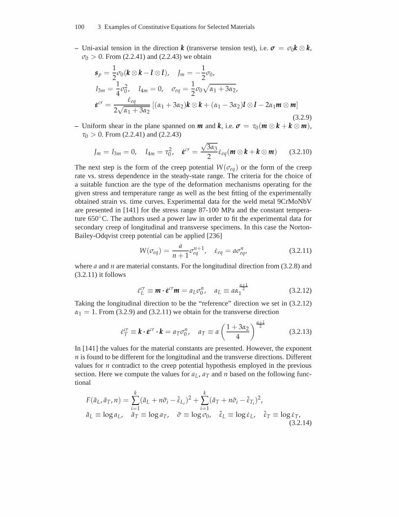
100 3 Examples of Constitutive Equations for Selected Materials
– Uni-axial tension in the directionkkk (transverse tension test), i.e.σσσ = σ0kkk ⊗ kkk,σ0 > 0. From (2.2.41) and (2.2.43) we obtain
sssp =1
2σ0(kkk ⊗ kkk − lll ⊗ lll), Jm = −1
2σ0,
I3m =1
4σ2
0 , I4m = 0, σeq =1
2σ0
√
α1 + 3α2,
εεεcr =εeq
2√
α1 + 3α2[(α1 + 3α2)kkk ⊗ kkk + (α1 − 3α2)lll ⊗ lll − 2α1mmm ⊗mmm]
(3.2.9)– Uniform shear in the plane spanned onmmm andkkk, i.e. σσσ = τ0(mmm ⊗ kkk + kkk ⊗ mmm),
τ0 > 0. From (2.2.41) and (2.2.43)
Jm = I3m = 0, I4m = τ20 , εεεcr =
√3α3
2εeq(mmm ⊗ kkk + kkk ⊗mmm) (3.2.10)
The next step is the form of the creep potentialW(σeq) or the form of the creeprate vs. stress dependence in the steady-state range. The criteria for the choice ofa suitable function are the type of the deformation mechanisms operating for thegiven stress and temperature range as well as the best fittingof the experimentallyobtained strain vs. time curves. Experimental data for the weld metal 9CrMoNbVare presented in [141] for the stress range 87-100 MPa and theconstant tempera-ture 650C. The authors used a power law in order to fit the experimentaldata forsecondary creep of longitudinal and transverse specimens.In this case the Norton-Bailey-Odqvist creep potential can be applied [236]
W(σeq) =a
n + 1σn+1
eq , εeq = aσneq, (3.2.11)
wherea andn are material constants. For the longitudinal direction from (3.2.8) and(3.2.11) it follows
εcrL ≡ mmm ··· εεεcrmmm = aLσn
0 , aL ≡ aαn+1
21 (3.2.12)
Taking the longitudinal direction to be the “reference” direction we set in (3.2.12)α1 = 1. From (3.2.9) and (3.2.11) we obtain for the transverse direction
εcrT ≡ kkk ··· εεεcr ··· kkk = aTσn
0 , aT ≡ a
(
1 + 3α2
4
) n+12
(3.2.13)
In [141] the values for the material constants are presented. However, the exponentn is found to be different for the longitudinal and the transverse directions. Differentvalues forn contradict to the creep potential hypothesis employed in the previoussection. Here we compute the values foraL, aT andn based on the following func-tional
F(aL, aT , n) =k
∑i=1
(aL + nσi − ˜εLi)2 +
k
∑i=1
(aT + nσi − ˜εTi)2,
aL ≡ log aL, aT ≡ log aT , σ ≡ log σ0, ˜εL ≡ log εL, ˜εT ≡ log εT ,(3.2.14)
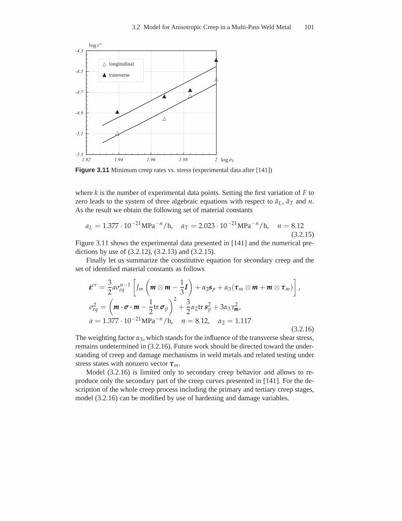
3.2 Model for Anisotropic Creep in a Multi-Pass Weld Metal 101
1 . 9 2 1 . 9 4 1 . 9 6 1 . 9 8 2- 5 . 3
- 5 . 1
- 4 . 9
- 4 . 7
- 4 . 5
- 4 . 3
log σ0
log εcr
longitudinal
transverse
Figure 3.11 Minimum creep rates vs. stress (experimental data after [141])
wherek is the number of experimental data points. Setting the first variation ofF tozero leads to the system of three algebraic equations with respect toaL, aT andn.As the result we obtain the following set of material constants
aL = 1.377 · 10−21MPa−n/h, aT = 2.023 · 10−21MPa−n/h, n = 8.12(3.2.15)
Figure 3.11 shows the experimental data presented in [141] and the numerical pre-dictions by use of (3.2.12), (3.2.13) and (3.2.15).
Finally let us summarize the constitutive equation for secondary creep and theset of identified material constants as follows
εεεcr =3
2aσn−1
eq
[
Jm
(
mmm ⊗mmm − 1
3III
)
+ α2sssp + α3(τττm ⊗mmm + mmm ⊗ τττm)
]
,
σ2eq =
(
mmm ··· σσσ ···mmm − 1
2tr σσσp
)2
+3
2α2tr sss2
p + 3α3τ2mmm,
a = 1.377 · 10−21MPa−n/h, n = 8.12, α2 = 1.117(3.2.16)
The weighting factorα3, which stands for the influence of the transverse shear stress,remains undetermined in (3.2.16). Future work should be directed toward the under-standing of creep and damage mechanisms in weld metals and related testing understress states with nonzero vectorτττm.
Model (3.2.16) is limited only to secondary creep behavior and allows to re-produce only the secondary part of the creep curves presented in [141]. For the de-scription of the whole creep process including the primary and tertiary creep stages,model (3.2.16) can be modified by use of hardening and damage variables.

102 3 Examples of Constitutive Equations for Selected Materials
4 Modeling of Creep in Structures
In Chapters 2 and 3 we introduced constitutive and evolutionequations for the mod-eling of creep in engineering materials. The objective of Chapt. 4 is the applicationof creep constitutive models to structural analysis. In Sect. 4.1 we start with thediscussion of aims and basic steps in modeling of creep in structures. In Sect. 4.2we formulate initial-boundary value problems describing creep behavior in three-dimensional solids and give an overview on numerical solution procedures. Sections4.3 – 4.4 are devoted to the review and evaluation of structural mechanics models ofbeams, plates and shells in the context of their applicability to the analysis of creepand long term strength. For several problems we develop closed-form solutions andspecial numerical solutions based on the Ritz method. The results are applied to ver-ify finite element solutions obtained by a general purpose finite element code and auser defined material subroutine. Special numerical examples are selected to illus-trate the influence of various discretisation parameters (mesh size, number of Gausspoints, etc.) on the solution accuracy. Furthermore, they allow to compare creep life-time predictions based on different structural mechanics models and related types offinite elements. To discuss the applicability of the developed techniques to real en-gineering problems an example of a spatial steam pipeline ispresented. Long termbehavior of the pipeline under constant internal pressure and constant temperatureis simulated by the finite element method. Numerical resultsare compared with thedata from engineering practice.
4.1 General Remarks
The aim of creep modeling is to reflect basic features of creepin structures includingthe development of inelastic deformations, relaxation andredistribution of stressesas well as the local reduction of material strength (see Sect. 1.2). A model shouldbe able to account for material deterioration processes in order to predict long termstructural behavior and to analyze critical zones of creep failure. Structural analysisunder creep conditions usually requires the following steps:
1. Assumptions must be made with regard to the geometry of thestructure, typesof loading and heating as well as kinematical constraints.
2. A suitable structural mechanics model must be applied based on the assump-tions concerning kinematics of deformations, types of internal forces (mo-ments) and related balance equations.
104 4 Modeling of Creep in Structures
3. A reliable constitutive model must be formulated to reflect time dependentcreep deformations and processes accompanying creep like hardening/recoveryand damage.
4. A mathematical model of the structural behavior (initial-boundary value prob-lem) must be formulated including the material independentequations, consti-tutive (evolution) equations as well as initial and boundary conditions.
5. Numerical solution procedures to solve non-linear initial-boundary value prob-lems must be developed.
6. The verification of the applied models must be performed including the struc-tural mechanics model, the constitutive model, the mathematical model as wellas the numerical methods and algorithms.
The first two steps are common within continuum mechanics andengineering me-chanics. Here, mathematical models of idealized solids andstructures are developedand investigated. Examples include the models of three-dimensional solids, beams,rods, plates and shells. The idealizations are related to the continuum hypothesis,cross section assumptions, etc. The above models were originally developed withinthe theory of linear elasticity, e.g. [126, 308]. In creep mechanics they are appliedtogether with constitutive and evolution equations describing idealized creep behav-ior (e.g. steady state creep) [77, 139, 173, 202, 234]. As mentioned in Sect. 1.1.2and Chapt. 2, many structural materials exhibit non-classical creep phenomena suchas different creep rates under tension and compression, stress state dependence oftertiary creep, damage induced anisotropy, etc. Consideration of such effects mayrequire various extensions of available structural mechanics models. For example,the concept of the stress free (neutral) plane widely used inthe theory of beams andplates becomes invalid in creep mechanics if the material shows different creep ratesunder tension and compression (see Sect. 1.2). Below we discuss the applicabilityof classical and refined models of beams, plates and shells tothe creep analysis.Bases on several examples we examine the accuracy of cross section assumptionsfor displacement and stress fields.
The mathematical model of creep in structure is the initial-boundary value prob-lem (IBVP) which usually includes partial differential equations describing kine-matics of deformation and balance of forces, ordinary differential equations de-scribing creep processes as well as initial and boundary conditions. The numeri-cal solution can be organized as follows, e.g. [77, 250]. Forknown values of thecreep strain tensor and internal state variables at a fixed time the boundary valueproblem (BVP) is solved. Here direct variational methods, e.g. the Ritz method, theGalerkin method, the finite element method are usually applied. In addition, a timestep procedure is required to integrate constitutive and evolution equations of creep.Below various methods are reviewed and discussed with respect to their efficiencyand numerical accuracy.
In recent years the finite element method has become the widely accepted toolfor structural analysis. The advantage of the finite elementmethod is the possibil-ity to model and analyze engineering structures with complex geometries, varioustypes of loadings and boundary conditions. General purposefinite element codes
4.1 General Remarks 105
ABAQUS, ADINA, ANSYS, COSMOS, etc. were developed to solve various prob-lems in solid mechanics. In application to the creep analysis one should take intoaccount that a general purpose constitutive equation whichallows to reflect thewhole set of creep and damage processes in structural materials over a wide rangeof loading and temperature conditions is not available at present. Therefore, a spe-cific constitutive model with selected internal state variables, special types of stressand temperature functions as well as material constants identified from availableexperimental data should be incorporated into the commercial finite element codeby writing a user defined material subroutine. Below the ANSYS finite elementcode is applied to the numerical analysis of creep in structures. In order to considerdamage processes the subroutines “usercreep” and “userout” are developed and im-plemented. The former serves to introduce constitutive equations with damage statevariables and corresponding evolution equations. The latter allows the postprocess-ing of damage, i.e. the creation of contour plots visualizing the damage distributions.
An important question in the creep analysis is that on reliability of the appliedmodels, numerical methods and obtained results. The reliability assessment mayrequire the following verification steps:
– Verification of developed finite element subroutines. To assess that the subrou-tines are correctly coded and implemented, results of finiteelement computa-tions must be compared with reference solutions of benchmark problems. Sev-eral benchmark problems have been proposed in [38] based on an in-house finiteelement code. Below we formulate and solve own benchmark problems includ-ing beams and transversely loaded plates. The advantage of these problems is thepossibility to obtain reference solutions by means of the Ritz method without afinite element discretisation. Furthermore, they allow to verify finite element sub-routines over a wide range of finite element types including beam, shell and solidtype elements.
– Verification of applied numerical methods. Here the problems of the suitable fi-nite element mesh density, the time step size and the time step control must beanalyzed. They are of particular importance in creep damagerelated simulations.Below these problems are discussed based on numerical testsand by means ofcomparison with reference solutions.
– Verification of constitutive and structural mechanics models. This step requirescreep testing of model structural components and the corresponding numericalanalysis by the use of the developed techniques. Examples ofrecent experimen-tal studies of creep in structures include beams [77], transversely loaded plates[163, 224], thin-walled tubes under internal pressure [164, 177], pressure vessels[103, 114], circumferentially notched bars [133]. Let us note that the experimen-tal data for model structures are usually limited to short-term creep tests. Thefinite element codes and subroutines are designed to analyzereal engineeringstructures. Therefore long-term analysis of several typical structures should beperformed and the results should be compared with data collected from engineer-ing practice of power and petrochemical plants. Below an example of the creepfinite element analysis for a spatial steam pipeline is discussed.
106 4 Modeling of Creep in Structures
4.2 Initial-Boundary Value Problems and GeneralSolution Procedures
The objective of this Section is to discuss the governing mechanical equations de-scribing creep in three-dimensional solids and related numerical solution proce-dures. The set of equations includes material independent equations, constitutiveand evolution equations, see Chapt. 2, as well as the initialand boundary condi-tions. The formulated IBVP must be solved by numerical methods. Explicit andimplicit time integration methods are reviewed with respect to their accuracy andefficiency. Within the time-step procedures, different possibilities are discussed tosolve linearized boundary value problems. The attention will be given to the varia-tional formulations and the use of direct variational methods.
4.2.1 Governing Equations
Let us consider a solid occupying the volumeV with the surfaceA. We assumethat the solid is fixed on the surface partAu and loaded by surface forces on thepart Ap. The position of a material point within the solid in the reference state isdescribed by the position vectorrrr(qi) = eeeiq
i, i = 1, 2, 3, whereeeei are basis vectorsand qi are coordinates (see Sect. A.2.1). The corresponding position in the actualstate can be characterized by the position vectorRRR(qi, t) or by the displacementvectoruuu(qi, t) = RRR(qi, t) − rrr(qi). The problem is to find the time sequence of theactual configurationsRRR(qi, t) as a result of external actions for a given time inter-val and∀qi ∈ V. The governing equations are discussed in continuum mechanicse.g. [29, 35, 44, 57, 108, 131, 178, 199]. Constitutive equations describing creepprocesses have been introduced in Chapt. 2. Besides the kinematical quantities, ad-ditional unknowns are the creep strain tensorεεεcr(qi, t) and the set of internal statevariablesHk(qi, t), k = 1, . . . , n andωl(qi, t), l = 1, . . . , m. They are introducedto characterize the current state of the material microstructure and to reflect the en-tire previous history of the creep process (see Sect. 2.1). In this section we limitour considerations to linearized kinematical equations inthe sense of infinitesimalstrains and displacements. Furthermore, we assume a classical non-polar contin-uum, quasi-static processes and isothermal conditions. The related comments weremade in Sect. 2.1.
The governing equations can be summarized as follows
– kinematical equations• strain-displacement relation
εεε =1
2
(
∇∇∇uuu + (∇∇∇uuu)T)
, qi ∈ V, (4.2.1)
whereεεε is the tensor of infinitesimal strains.• compatibility condition
∇∇∇××× (∇∇∇× εεε)T = 000, qi ∈ V, (4.2.2)
4.2 Initial-Boundary Value Problems and General Solution Procedures 107
– equilibrium conditions
∇∇∇··· σσσ + ρ fff = 000, σσσ× = 000, qi ∈ V, (4.2.3)
whereρ is the material density andfff is the density of volumetric forces– boundary conditions
uuu = uuu, qi ∈ Au,
σσσ ··· ννν = ppp, qi ∈ Ap,(4.2.4)
whereuuu is the given displacement vector andppp is the vector of given surface forcesandννν is the outward unit normal toAp. The vectorsfff , ppp anduuu can be, in general,functions of coordinates and time.
With the assumption of infinitesimal strains the additive decomposition of thetotal strain into elastic, thermal and creep parts is usually postulated
εεε = εεεel + εεεth + εεεcr (4.2.5)
The constitutive equation for the stress tensor can be assumed in the form of thegeneralized Hooke’s law as follows
σσσ = (4)CCC ······ (εεε − εεεth − εεεcr) (4.2.6)
In the case of isotropic elasticity the tensor(4)CCC takes the form
(4)CCC = λIII ⊗ III + µ(eeek ⊗ III ⊗ eeek + eeei ⊗ eeek ⊗ eeei ⊗ eeek), (4.2.7)
whereλ andµ are the Lame’s constants
µ = G =E
2(1 + ν), λ =
νE
(1 + ν)(1 − 2ν)
E is the Young’s modulus,G is the shear modulus,ν is the Poisson’s ratio.If an isotropic solid is heated from the reference temperature T0 up to T, the
thermal part of the strain tensor is
εεεth = αT∆TIII, ∆T ≡ T − T0, (4.2.8)
whereαT is the coefficient of the thermal expansion.∆T can be a function of coor-dinates and time too.
The constitutive equations for the creep rate and evolutionequations for internalstate variables are discussed in Chapt. 2. Here we will use the rate equations in thefollowing form
εεεcr =∂Φ(
σeq(σσσ), Hk, ωl; T)
∂σσσ, k = 1, . . . , n, l = 1, . . . , m,
Hk = Hk
(
σHeq(σσσ), Hk, ωl; T
)
, ωl = ωl
(
σωeq(σσσ), Hk, ωl; T
)(4.2.9)

108 4 Modeling of Creep in Structures
The hardening variablesHk and the damage variablesωl can be scalars or tensors.For the creep strain as well as for the set of hardening and damage variables theinitial conditions must be specified. Let us assume
εεεcr∣
∣
∣
t=0= 000, Hk
∣
∣
∣
t=0= H0
k , ωl
∣
∣
∣
t=0= ω0
l , (4.2.10)
whereH0k andω0
l are the initial values of the hardening and the damage parameters.Equations (4.2.1) – (4.2.10) describe the quasi-static creep process in a solid.
4.2.2 Vector-Matrix Representation
To formulate initial-boundary value problems and numerical solution procedureslet us rewrite Eqs (4.2.1) – (4.2.10) in the vector-matrix notation. For the sake ofbrevity we introduce the Cartesian coordinatesx1, x2, x3. The Cartesian componentsof vectors and tensors can be collected into the following “numerical” vectors andmatrices:
Stress vector σσσ σσσT = [σ11 σ22 σ33 σ12 σ23 σ31]
Strain vector εεε εεεT = [ε11 ε22 ε33 γ12 γ23 γ31]
Displacement vector uuu uuuT = [u1 u2 u3]
Vector of creep strains εεεcr εεεcrT = [εcr11 εcr
22 εcr33 γcr
12 γcr23 γcr
31]
Vector of internal variables ξξξ ξξξT = [H1 H2 . . . Hn ω1 ω2 . . . ωm]
Vector of thermal strains εεεth εεεthT= [αT∆T αT∆T αT∆T 0 0 0]
Vector of body forces fff fffT
= [ f1 f2 f3]
Vector of surface forces ppp pppT = [p1 p2 p3]
Stress vectorσσσννν onνννdA σσσTννν = [σν1
σν2 σν3 ]
Normal vector ννν νννT = [ν1 ν2 ν3],νi = cos(ννν, xi)
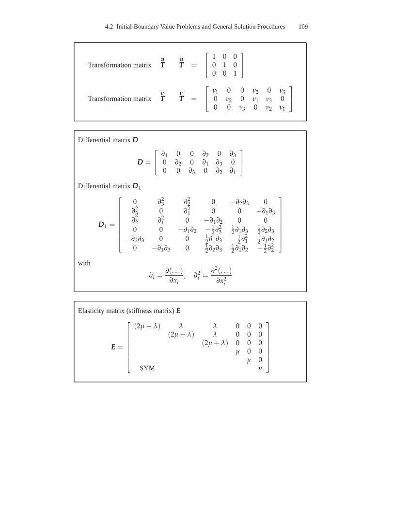
4.2 Initial-Boundary Value Problems and General Solution Procedures 109
Transformation matrixuuuTTT
uuuTTT =
1 0 00 1 00 0 1
Transformation matrixσσσTTT
σσσTTT =
ν1 0 0 ν2 0 ν3
0 ν2 0 ν1 ν3 00 0 ν3 0 ν2 ν1
Differential matrixDDD
DDD =
∂1 0 0 ∂2 0 ∂3
0 ∂2 0 ∂1 ∂3 00 0 ∂3 0 ∂2 ∂1
Differential matrixDDD1
DDD1 =
0 ∂23 ∂2
2 0 −∂2∂3 0
∂23 0 ∂2
1 0 0 −∂1∂3
∂22 ∂2
1 0 −∂1∂2 0 0
0 0 −∂1∂2 − 12 ∂2
312 ∂1∂3
12 ∂2∂3
−∂2∂3 0 0 12 ∂1∂3 − 1
2 ∂21
12 ∂1∂2
0 −∂1∂3 0 12 ∂2∂3
12 ∂1∂2 − 1
2 ∂22
with
∂i =∂(. . .)
∂xi, ∂2
i =∂2(. . .)
∂x2i
Elasticity matrix (stiffness matrix)EEE
EEE =
(2µ + λ) λ λ 0 0 0(2µ + λ) λ 0 0 0
(2µ + λ) 0 0 0µ 0 0
µ 0SYM µ
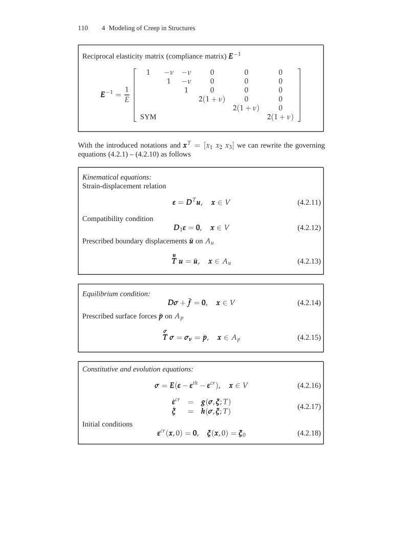
110 4 Modeling of Creep in Structures
Reciprocal elasticity matrix (compliance matrix)EEE−1
EEE−1 =1
E
1 −ν −ν 0 0 01 −ν 0 0 0
1 0 0 02(1 + ν) 0 0
2(1 + ν) 0SYM 2(1 + ν)
With the introduced notations andxxxT = [x1 x2 x3] we can rewrite the governingequations (4.2.1) – (4.2.10) as follows
Kinematical equations:Strain-displacement relation
εεε = DDDTuuu, xxx ∈ V (4.2.11)
Compatibility conditionDDD1εεε = 000, xxx ∈ V (4.2.12)
Prescribed boundary displacementsuuu on Au
uuuTTT uuu = uuu, xxx ∈ Au (4.2.13)
Equilibrium condition:DσDσDσ + fff = 000, xxx ∈ V (4.2.14)
Prescribed surface forcesppp on Ap
σσσTTT σσσ = σσσννν = ppp, xxx ∈ Ap (4.2.15)
Constitutive and evolution equations:
σσσ = EEE(εεε − εεεth − εεεcr), xxx ∈ V (4.2.16)
εεεcr = ggg(σσσ, ξξξ; T)ξξξ = hhh(σσσ, ξξξ; T)
(4.2.17)
Initial conditionsεεεcr(xxx, 0) = 000, ξξξ(xxx, 0) = ξξξ0 (4.2.18)
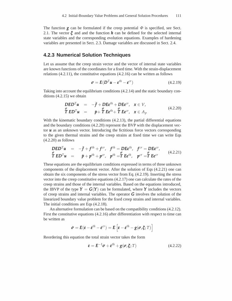
4.2 Initial-Boundary Value Problems and General Solution Procedures 111
The functionggg can be formulated if the creep potentialΦ is specified, see Sect.2.1. The vectorξξξ and and the functionhhh can be defined for the selected internalstate variables and the corresponding evolution equations. Examples of hardeningvariables are presented in Sect. 2.3. Damage variables are discussed in Sect. 2.4.
4.2.3 Numerical Solution Techniques
Let us assume that the creep strain vector and the vector of internal state variablesare known functions of the coordinates for a fixed time. With the strain-displacementrelations (4.2.11), the constitutive equations (4.2.16) can be written as follows
σσσ = EEE(DDDTuuu − εεεth − εεεcr) (4.2.19)
Taking into account the equilibrium conditions (4.2.14) and the static boundary con-ditions (4.2.15) we obtain
DDDEEEDDDTuuu = − fff + DDDEEEεεεth + DDDEEEεεεcr, xxx ∈ V,σσσTTT EEEDDDTuuu = ppp+
σσσTTT EEEεεεth+
σσσTTT EEEεεεcr, xxx ∈ Ap
(4.2.20)
With the kinematic boundary conditions (4.2.13), the partial differential equationsand the boundary conditions (4.2.20) represent the BVP withthe displacement vec-tor uuu as an unknown vector. Introducing the fictitious force vectors correspondingto the given thermal strains and the creep strains at fixed time we can write Eqs(4.2.20) as follows
DDDEEEDDDTuuu = − fff + fff th + fff cr, fff th = DDDEEEεεεth, fff cr = DDDEEEεεεcr,σσσTTT EEEDDDTuuu = ppp + pppth + pppcr, pppth =
σσσTTT EEEεεεth, pppcr =
σσσTTT EEEεεεcr
(4.2.21)
These equations are the equilibrium conditions expressed in terms of three unknowncomponents of the displacement vector. After the solution of Eqs (4.2.21) one canobtain the six components of the stress vector from Eq. (4.2.19). Inserting the stressvector into the creep constitutive equations (4.2.17) one can calculate the rates of thecreep strains and those of the internal variables. Based on the equations introduced,the IBVP of the typeYYY = GGG(YYY) can be formulated, whereYYY includes the vectorsof creep strains and internal variables. The operatorGGG involves the solution of thelinearized boundary value problem for the fixed creep strains and internal variables.The initial conditions are Eqs (4.2.18).
An alternative formulation can be based on the compatibility conditions (4.2.12).First the constitutive equations (4.2.16) after differentiation with respect to time canbe written as
σσσ = EEE(εεε − εεεth − εεεcr) = EEE[
εεε − εεεth − ggg(σσσ, ξξξ; T)]
Reordering this equation the total strain vector takes the form
εεε = EEE−1σσσ + εεεth + ggg(σσσ, ξξξ; T) (4.2.22)
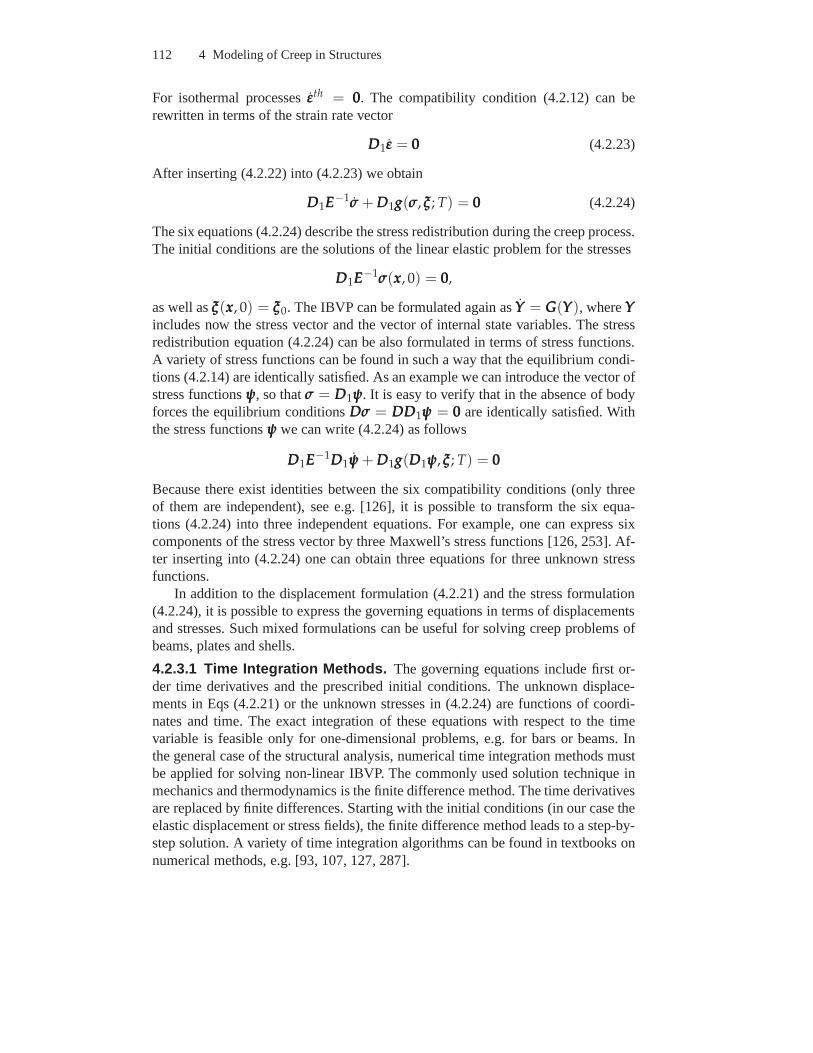
112 4 Modeling of Creep in Structures
For isothermal processesεεεth = 000. The compatibility condition (4.2.12) can berewritten in terms of the strain rate vector
DDD1εεε = 000 (4.2.23)
After inserting (4.2.22) into (4.2.23) we obtain
DDD1EEE−1σσσ + DDD1ggg(σσσ, ξξξ; T) = 000 (4.2.24)
The six equations (4.2.24) describe the stress redistribution during the creep process.The initial conditions are the solutions of the linear elastic problem for the stresses
DDD1EEE−1σσσ(xxx, 0) = 000,
as well asξξξ(xxx, 0) = ξξξ0. The IBVP can be formulated again asYYY = GGG(YYY), whereYYYincludes now the stress vector and the vector of internal state variables. The stressredistribution equation (4.2.24) can be also formulated interms of stress functions.A variety of stress functions can be found in such a way that the equilibrium condi-tions (4.2.14) are identically satisfied. As an example we can introduce the vector ofstress functionsψψψ, so thatσσσ = DDD1ψψψ. It is easy to verify that in the absence of bodyforces the equilibrium conditionsDDDσσσ = DDDDDD1ψψψ = 000 are identically satisfied. Withthe stress functionsψψψ we can write (4.2.24) as follows
DDD1EEE−1DDD1ψψψ + DDD1ggg(DDD1ψψψ, ξξξ; T) = 000
Because there exist identities between the six compatibility conditions (only threeof them are independent), see e.g. [126], it is possible to transform the six equa-tions (4.2.24) into three independent equations. For example, one can express sixcomponents of the stress vector by three Maxwell’s stress functions [126, 253]. Af-ter inserting into (4.2.24) one can obtain three equations for three unknown stressfunctions.
In addition to the displacement formulation (4.2.21) and the stress formulation(4.2.24), it is possible to express the governing equationsin terms of displacementsand stresses. Such mixed formulations can be useful for solving creep problems ofbeams, plates and shells.
4.2.3.1 Time Integration Methods. The governing equations include first or-der time derivatives and the prescribed initial conditions. The unknown displace-ments in Eqs (4.2.21) or the unknown stresses in (4.2.24) arefunctions of coordi-nates and time. The exact integration of these equations with respect to the timevariable is feasible only for one-dimensional problems, e.g. for bars or beams. Inthe general case of the structural analysis, numerical timeintegration methods mustbe applied for solving non-linear IBVP. The commonly used solution technique inmechanics and thermodynamics is the finite difference method. The time derivativesare replaced by finite differences. Starting with the initial conditions (in our case theelastic displacement or stress fields), the finite difference method leads to a step-by-step solution. A variety of time integration algorithms canbe found in textbooks onnumerical methods, e.g. [93, 107, 127, 287].
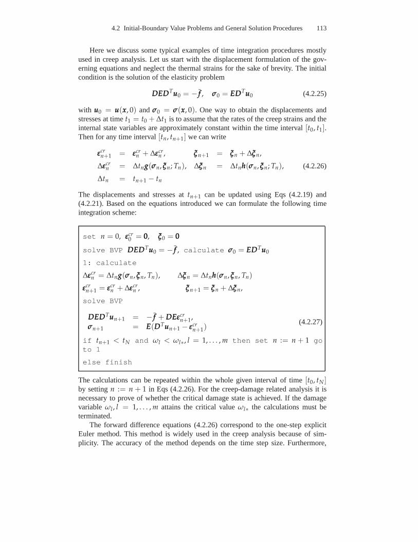
4.2 Initial-Boundary Value Problems and General Solution Procedures 113
Here we discuss some typical examples of time integration procedures mostlyused in creep analysis. Let us start with the displacement formulation of the gov-erning equations and neglect the thermal strains for the sake of brevity. The initialcondition is the solution of the elasticity problem
DDDEEEDDDTuuu0 = − fff , σσσ0 = EEEDDDTuuu0 (4.2.25)
with uuu0 = uuu(xxx, 0) andσσσ0 = σσσ(xxx, 0). One way to obtain the displacements andstresses at timet1 = t0 + ∆t1 is to assume that the rates of the creep strains and theinternal state variables are approximately constant within the time interval[t0, t1].Then for any time interval[tn, tn+1] we can write
εεεcrn+1 = εεεcr
n + ∆εεεcrn , ξξξn+1 = ξξξn + ∆ξξξn,
∆εεεcrn = ∆tnggg(σσσn, ξξξn; Tn), ∆ξξξn = ∆tnhhh(σσσn, ξξξn; Tn),
∆tn = tn+1 − tn
(4.2.26)
The displacements and stresses attn+1 can be updated using Eqs (4.2.19) and(4.2.21). Based on the equations introduced we can formulate the following timeintegration scheme:
set n = 0, εεεcr0 = 000, ξξξ0 = 000
solve BVP DDDEEEDDDTuuu0 = − fff , calculate σσσ0 = EEEDDDTuuu0
1: calculate
∆εεεcrn = ∆tnggg(σσσn, ξξξn, Tn), ∆ξξξn = ∆tnhhh(σσσn, ξξξn, Tn)
εεεcrn+1 = εεεcr
n + ∆εεεcrn , ξξξn+1 = ξξξn + ∆ξξξn,
solve BVP
DDDEEEDDDTuuun+1 = − fff + DDDEEEεεεcrn+1,
σσσn+1 = EEE(DDDTuuun+1 − εεεcrn+1)
(4.2.27)
if tn+1 < tN and ωl < ωl∗, l = 1, . . . , m then set n := n + 1 goto 1
else finish
The calculations can be repeated within the whole given interval of time [t0, tN ]by settingn := n + 1 in Eqs (4.2.26). For the creep-damage related analysis it isnecessary to prove of whether the critical damage state is achieved. If the damagevariable ωl, l = 1, . . . , m attains the critical valueωl∗ the calculations must beterminated.
The forward difference equations (4.2.26) correspond to the one-step explicitEuler method. This method is widely used in the creep analysis because of sim-plicity. The accuracy of the method depends on the time step size. Furthermore,
114 4 Modeling of Creep in Structures
this method is conditionally stable that means that the stability is restricted to smalltime steps. Therefore stable results can be obtained only for ∆t ≤ ∆tcrit. There isno general recipe how to control the time step size by the use the one step explicitmethod. For example, in [338] it is recommended to compute the time step size fromthe condition that the increment of the creep strain does notexceed one half of theelastic strain, i.e.
∆tnggg(σσσn, ξξξn; Tn) ≤ 1
2EEE−1σσσn
A further restriction is connected with the assumption thatthe stresses have to beconstant within the time interval[tn, tn+1]. Therefore this method can be recom-mended for structural analysis under constant or monotonicloading and tempera-ture conditions only. In the case of loading jumps or cyclic loading changes verysmall time steps are necessary in order to provide a stable solution.
One way to improve the accuracy of time-dependent solutionsis the use ofmulti-step methods of the Runge-Kutta type, see e.g. [77, 107, 127]. These explicitmethods are conditionally stable as well. However, they provide higher order ac-curacy if compared with the one-step forward difference method. Furthermore, forthe creep-damage related analysis the so-called embedded methods [127], which al-low to control the time step size, can be recommended. In [17,18] the embeddedfourth order Kutta-Merson method has been applied to creep problems of shells ofrevolution.
The next possibility to improve the one-step method is the use of the generalizedtrapezoidal rule [93]
εεεcrn+1 = εεεcr
n + ∆t[
(1 − θ)εεεcrn + θεεεcr
n+1
]
,
ξξξn+1 = ξξξn + ∆t[
(1 − θ)ξξξn + θξξξn+1
]
,(4.2.28)
whereθ (0 ≤ θ ≤ 1) is the parameter controlling the stability. The rule (4.2.28)includes different well-known methods as special cases. Setting θ = 0 the forwarddifference explicit Euler method (4.2.26) follows. Forθ > 0 we obtain a variety ofimplicit methods: forθ = 1/2 - the trapezoidal rule (Crank-Nicolson method), andfor θ = 1 the backward difference method (implicit Euler method). The advantageof the implicit methods is their unconditional stability that means that the solutionwill be stable independently on the time step size. The pricefor the unconditionalstability is the necessity to solve non-linear equations ateach time step. Equations(4.2.28) can be rewritten as follows
εεεcrn+1 = εεεcr
n + ∆εεεcrn ,
ξξξn+1 = ξξξn + ∆ξξξn,
∆εεεcrn = ∆tn [(1 − θ)ggg(σσσn, ξξξn; Tn) + θggg(σσσn+1, ξξξn+1, Tn+1)] ,
∆ξξξn = ∆tn [(1 − θ)hhh(σσσn, ξξξn; Tn) + θhhh(σσσn+1, ξξξn+1, Tn+1)]
(4.2.29)
Equations (4.2.29) are non-linear with respect toξξξn+1 for θ > 0. Note that for amaterial model with strain hardening, the vectorξξξn includes the equivalent creep
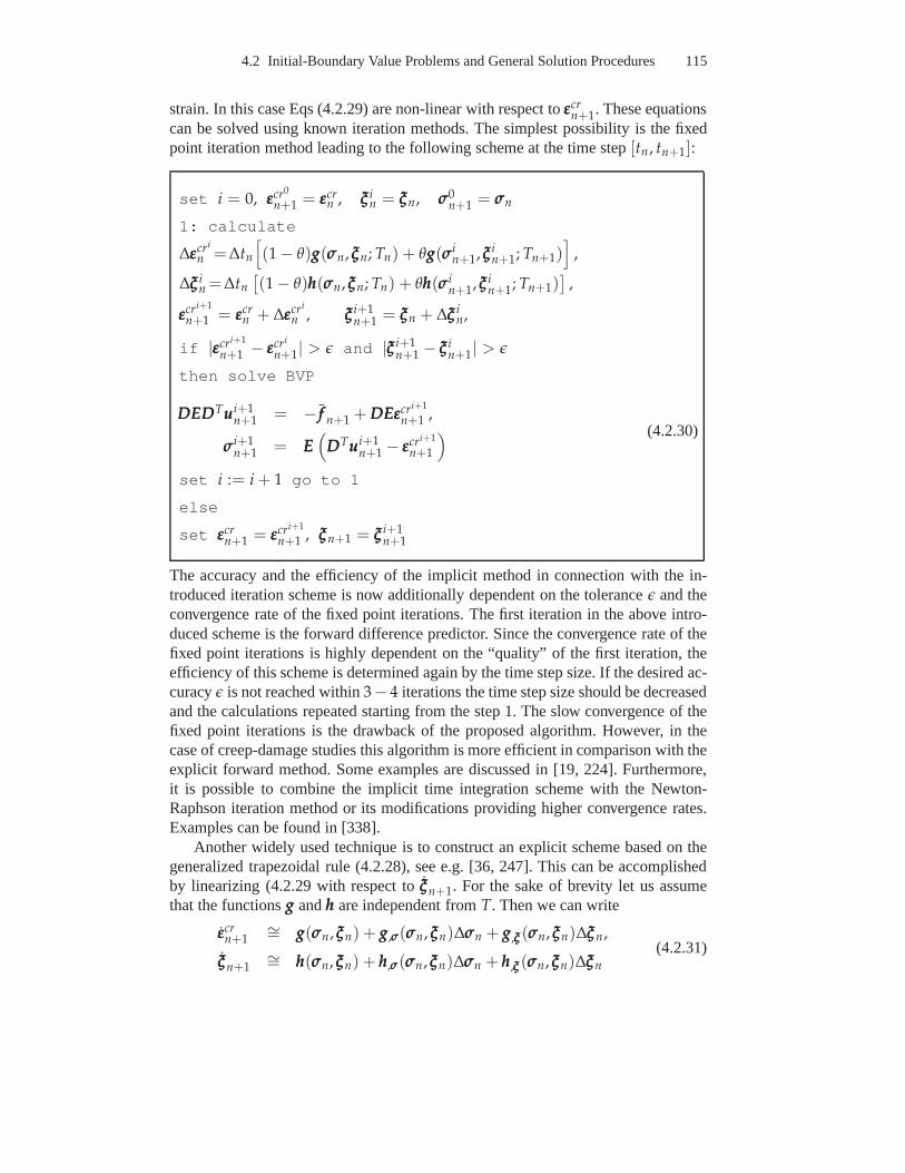
4.2 Initial-Boundary Value Problems and General Solution Procedures 115
strain. In this case Eqs (4.2.29) are non-linear with respect to εεεcrn+1. These equations
can be solved using known iteration methods. The simplest possibility is the fixedpoint iteration method leading to the following scheme at the time step[tn, tn+1]:
set i = 0, εεεcr0
n+1 = εεεcrn , ξξξ i
n = ξξξn, σσσ0n+1 = σσσn
1: calculate
∆εεεcri
n =∆tn
[
(1 − θ)ggg(σσσn, ξξξn; Tn) + θggg(σσσin+1, ξξξ i
n+1; Tn+1)]
,
∆ξξξ in =∆tn
[
(1 − θ)hhh(σσσn, ξξξn; Tn) + θhhh(σσσin+1, ξξξ i
n+1; Tn+1)]
,
εεεcri+1
n+1 = εεεcrn + ∆εεεcri
n , ξξξ i+1n+1 = ξξξn + ∆ξξξ i
n,
if |εεεcri+1
n+1 − εεεcri
n+1| > ǫ and |ξξξ i+1n+1 − ξξξ i
n+1| > ǫ
then solve BVP
DDDEEEDDDTuuui+1n+1 = − fff n+1 + DDDEEEεεεcri+1
n+1 ,
σσσi+1n+1 = EEE
(
DDDTuuui+1n+1 − εεεcri+1
n+1
) (4.2.30)
set i := i + 1 go to 1
else
set εεεcrn+1 = εεεcri+1
n+1 , ξξξn+1 = ξξξ i+1n+1
The accuracy and the efficiency of the implicit method in connection with the in-troduced iteration scheme is now additionally dependent onthe toleranceǫ and theconvergence rate of the fixed point iterations. The first iteration in the above intro-duced scheme is the forward difference predictor. Since theconvergence rate of thefixed point iterations is highly dependent on the “quality” of the first iteration, theefficiency of this scheme is determined again by the time stepsize. If the desired ac-curacyǫ is not reached within3− 4 iterations the time step size should be decreasedand the calculations repeated starting from the step 1. The slow convergence of thefixed point iterations is the drawback of the proposed algorithm. However, in thecase of creep-damage studies this algorithm is more efficient in comparison with theexplicit forward method. Some examples are discussed in [19, 224]. Furthermore,it is possible to combine the implicit time integration scheme with the Newton-Raphson iteration method or its modifications providing higher convergence rates.Examples can be found in [338].
Another widely used technique is to construct an explicit scheme based on thegeneralized trapezoidal rule (4.2.28), see e.g. [36, 247].This can be accomplishedby linearizing (4.2.29 with respect toξξξn+1. For the sake of brevity let us assumethat the functionsggg andhhh are independent fromT. Then we can write
εεεcrn+1
∼= ggg(σσσn, ξξξn) + ggg,σσσ(σσσn, ξξξn)∆σσσn + ggg,ξξξ(σσσn, ξξξn)∆ξξξn,
ξξξn+1∼= hhh(σσσn, ξξξn) + hhh,σσσ(σσσn, ξξξn)∆σσσn + hhh,ξξξ(σσσn, ξξξn)∆ξξξn
(4.2.31)
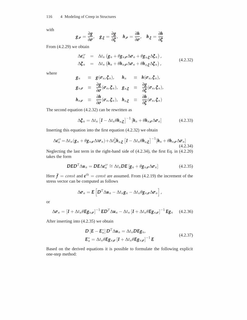
116 4 Modeling of Creep in Structures
with
ggg,σσσ =∂ggg
∂σσσ, ggg,ξξξ =
∂ggg
∂ξξξ, hhh,σσσ =
∂hhh
∂σσσ, hhh,ξξξ =
∂hhh
∂ξξξ
From (4.2.29) we obtain
∆εεεcrn = ∆tn
(
gggn + θgggn,σσσ∆σσσn + θgggn,ξξξ ∆ξξξn
)
,
∆ξξξn = ∆tn(
hhhn + θhhhn,σσσ∆σσσn + θhhhn,ξξξ ∆ξξξn)
,(4.2.32)
wheregggn ≡ ggg(σσσn, ξξξn), hhhn ≡ hhh(σσσn, ξξξn),
gggn,σσσ ≡ ∂ggg
∂σσσ(σσσn, ξξξn), gggn,ξξξ ≡ ∂ggg
∂ξξξ(σσσn, ξξξn),
hhhn,σσσ ≡ ∂hhh
∂σσσ(σσσn, ξξξn), hhhn,ξξξ ≡ ∂hhh
∂ξξξ(σσσn, ξξξn)
The second equation (4.2.32) can be rewritten as
∆ξξξn = ∆tn[
III − ∆tnθhhhn,ξξξ
]−1[hhhn + θhhhn,σσσ∆σσσn] (4.2.33)
Inserting this equation into the first equation (4.2.32) we obtain
∆εεεcrn =∆tn(gggn + θgggn,σσσ∆tσσσn)+∆t2
nhhhn,ξξξ
[
III − ∆tnθhhhn,ξξξ
]−1[hhhn + θhhhn,σσσ∆σσσn]
(4.2.34)Neglecting the last term in the right-hand side of (4.2.34),the first Eq. in (4.2.20)takes the form
DDDEEEDDDT∆uuun = DDDEEE∆εεεcrn∼= ∆tnDDDEEE [gggn + θgggn,σσσ∆σσσn] (4.2.35)
Here fff = const andεεεth = const are assumed. From (4.2.19) the increment of thestress vector can be computed as follows
∆σσσn = EEE[
DDDT∆uuun − ∆tngggn − ∆tnθgggn,σσσ∆σσσn
]
,
or
∆σσσn = [III + ∆tnθEEEgggn,σσσ]−1 EEEDDDT∆uuun − ∆tn [III + ∆tnθEEEgggn,σσσ]−1 EEEgggn (4.2.36)
After inserting into (4.2.35) we obtain
DDD [EEE − EEE∗n] DDDT∆uuun = ∆tnDDDEEEgggn,
EEE∗n = ∆tnθEEEgggn,σσσ [III + ∆tnθEEEgggn,σσσ]−1 EEE
(4.2.37)
Based on the derived equations it is possible to formulate the following explicitone-step method:
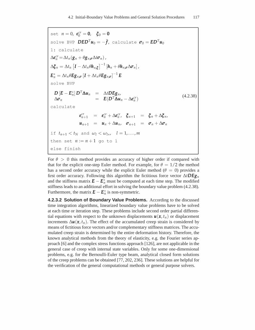
4.2 Initial-Boundary Value Problems and General Solution Procedures 117
set n = 0, εεεcr0 = 000, ξξξ0 = 000
solve BVP DDDEEEDDDTuuu0 = − fff , calculate σσσ0 = EEEDDDTuuu0
1: calculate
∆εεεcrn =∆tn(gggn + θgggn,σσσ∆tσσσn) ,
∆ξξξn = ∆tn
[
III − ∆tnθhhhn,ξξξ
]−1[hhhn + θhhhn,σσσ∆σσσn] ,
EEE∗n = ∆tnθEEEgggn,σσσ [III + ∆tnθEEEgggn,σσσ]−1 EEE
solve BVP
DDD [EEE − EEE∗n] DDDT∆∆∆uuun = ∆tDDDEEEgggn,
∆σσσn = EEE(DDDT∆∆∆uuun − ∆εεεcrn )
(4.2.38)
calculate
εεεcrn+1 = εεεcr
n + ∆εεεcrn , ξξξn+1 = ξξξn + ∆ξξξn,
uuun+1 = uuun + ∆uuun, σσσn+1 = σσσn + ∆σσσn
if tn+1 < tN and ωl < ωl∗, l = 1, . . . , m
then set n := n + 1 go to 1
else finish
For θ > 0 this method provides an accuracy of higher order if comparedwiththat for the explicit one-step Euler method. For example, for θ = 1/2 the methodhas a second order accuracy while the explicit Euler method (θ = 0) provides afirst order accuracy. Following this algorithm the fictitious force vector∆tDDDEEEgggn
and the stiffness matrixEEE − EEE∗n must be computed at each time step. The modified
stiffness leads to an additional effort in solving the boundary value problem (4.2.38).Furthermore, the matrixEEE − EEE∗
n is non-symmetric.
4.2.3.2 Solution of Boundary Value Problems. According to the discussedtime integration algorithms, linearized boundary value problems have to be solvedat each time or iteration step. These problems include second order partial differen-tial equations with respect to the unknown displacementsuuu(xxx, tn) or displacementincrements∆uuu(xxx, tn). The effect of the accumulated creep strain is considered bymeans of fictitious force vectors and/or complementary stiffness matrices. The accu-mulated creep strain is determined by the entire deformation history. Therefore, theknown analytical methods from the theory of elasticity, e.g. the Fourier series ap-proach [6] and the complex stress functions approach [126],are not applicable in thegeneral case of creep with internal state variables. Only for some one-dimensionalproblems, e.g. for the Bernoulli-Euler type beam, analytical closed form solutionsof the creep problems can be obtained [77, 202, 236]. These solutions are helpful forthe verification of the general computational methods or general purpose solvers.
118 4 Modeling of Creep in Structures
In what follows let us briefly discuss the numerical methods recently used increep mechanics. These methods are:
– the finite difference method,– the direct variational methods and– the boundary element method.
Applying the finite difference method the partial differential operators are replacedby finite differences leading to the solution of algebraic equations instead of thepartial differential ones. The utilization is mostly efficient for creep problems lead-ing to ordinary differential equations. Examples include axi-symmetrically loadedshells of revolution and circular plates [17, 18, 30, 60, 61,80, 82, 221, 255, 291].
The widely used approach is based on the variational formulations of the creepproblem. Starting from appropriate variational functionals the following direct vari-ational methods can be applied: the Ritz method, the Galerkin method and theVlasov-Kantorovich method. We will briefly discuss the variational formulationsand the classical variational methods in the next subsection. The most powerfulvariational method for the structural analysis is the finiteelement method [37, 338]which is the basis of commercial general purpose solvers, e.g., ABAQUS, ADINA,ANSYS, COSMOS, etc. The possibility to incorporate a creep material model withinternal state variables is available in commercial codes.The implementation can beperformed by writing a user defined material subroutine.
The boundary element method is based on the transformation of the partial dif-ferential equations into boundary integral equations. In order to solve these equa-tions the boundary of the domain is divided into finite elements. As a result a setof algebraic equations with respect to the vector of displacements (tractions) in thediscretisation points of the boundary can be obtained. In the case of creep an ad-ditional domain discretisation is necessary in order to store the components of thecreep strain vector [39]. For details of the boundary element technique we refer to[78, 130, 253].
4.2.3.3 Variational Formulations and Procedures. Variational formulationsare widely used in several problems of solid mechanics. Theyare the basis for directvariational methods, e.g. the Ritz method, the Galerkin method, the finite elementmethod. With respect to the type of the BVP, different variational functionals havebeen proposed. Here let us consider a variational functional in terms of the displace-ment vector. Letuuu(qi, t) be the solution of the BVP (4.2.1) - (4.2.6) under givenεεεcr.Let δuuu be the vector of virtual displacements satisfying the kinematic boundaryconditions (4.2.4). Starting from the equilibrium condition (4.2.3) we can write
∫
V
(∇∇∇ ··· σσσ + ρ fff ) ··· δuuudV = 0 (4.2.39)
According to (A.2.2)∫
V
(∇∇∇ ··· σσσ) ··· δuuudV =∫
V
[
∇∇∇ ··· (σσσ ··· δuuu) − σσσ ······ (∇∇∇δuuu)T]
dV (4.2.40)
4.2 Initial-Boundary Value Problems and General Solution Procedures 119
Applying the divergence theorem (see Sect. A.2.3) and the static boundary condi-tions (4.2.4) we obtain
∫
V
∇∇∇ ··· (σσσ ··· δuuu)dV =∫
A
(ννν ··· σσσ) ··· δuuudA =∫
Ap
ppp ··· δuuudA (4.2.41)
With σσσ ······ (∇∇∇δuuu)T = σσσ ······ δ(∇∇∇uuu)T = σσσ ······ δεεε, (4.2.40) and (4.2.41), Eq. (4.2.39) takesthe form
∫
V
σσσ ······ δεεεdV −∫
V
ρ fff ··· δuuudV −∫
Ap
ppp ··· δuuudA = 0, (4.2.42)
or
δWi + δWe = 0, δWi = −∫
V
σσσ ······ δεεεdV, δWe =∫
V
f ··· δuuudV +∫
Ap
ppp ··· δuuudA
(4.2.43)The principle of virtual displacements (4.2.43) states that if a deformable systemis in equilibrium then the sum of the virtual work of externalactionsδWe and thevirtual work of internal forcesδWi is equal to zero, e.g., [6, 253, 321]. With theconstitutive equation (4.2.6)
σσσ ······ δεεε =(
(4)CCC ······ (εεε − εεεcr − εεεth))
······ δεεε
=1
2δ(εεε ······ (4)CCC ······ εεε) − (εεεcr + εεεth) ······ (4)CCC ······ δεεε
the variational equation (4.2.43) can be formulated as follows
δ
1
2
∫
V
εεε ······ (4)CCC ······ εεεdV −∫
V
fff ··· uuudV −∫
Ap
ppp ··· uuudA
−∫
V
(εεεcr + εεεth) ······ (4)CCC ······ εεεdV
= 0
or δΠ(uuu) = 0 with
Π(uuu) =1
2
∫
V
εεε ······ (4)CCC ······ εεεdV −∫
V
fff ··· uuudV −∫
Ap
ppp ··· uuudA
−∫
V
(εεεcr + εεεth) ······ (4)CCC ······ εεεdV(4.2.44)
Applying the vector-matrix notation we can write
Π(uuu) =1
2
∫
V
(DDDTuuu)TEEEDDDTuuudV −∫
V
fffT
uuudV −∫
Ap
pppTuuudA
−∫
V
εεεthEEEDDDTuuudV −∫
V
εεεcrEEEDDDTuuudV(4.2.45)
120 4 Modeling of Creep in Structures
It is easy to verify that from the conditionδΠ(uuu) = 0 follows the partial differentialequation with respect to the displacement vector and the static boundary condition(4.2.20).
The variational functional (4.2.45) has been derived from the principle of vir-tual displacements. By analogy a variational functional interms of stresses or stressfunctions can be formulated providing Eqs (4.2.24) as Eulerequations. Furthermore,a mixed variational formulation in terms of displacements and stresses can be conve-nient for numerous structural mechanics problems. In [18, 224] a mixed variationalfunctional has been utilized for the solution of the von Karman type plate equations.In [16, 20, 225] a mixed formulation has been applied to derive the first order sheardeformation beam equations.
To solve the variational problem classical direct variational methods can be uti-lized. Let us illustrate the application of the Ritz method to the variational functional(4.2.45). The approximate solution for the displacement vector uuu is presented in theform of series
uk =N
∑i=1
akiφki(x1, x2, x3), k = 1, 2, 3 (4.2.46)
(no summation overk) or
uuu ≡
u1
u2
u3
=
aaaT1 φφφ1
aaaT2 φφφ2
aaaT3 φφφ3
=
φφφ1 000 000
000 φφφ2 000
000 000 φφφ3
T
aaa1
aaa2
aaa3
= GGGTaaa, (4.2.47)
whereφφφk are vectors of the trial (basis or shape) functions which should be speci-fied a priori andaaak are vectors of unknown (free) parameters. The functionsφki in(4.2.46) must be linearly independent and satisfy the kinematical boundary condi-tions. Furthermore, the set of these functions must be complete in order to providethe convergence ofuuu as N → ∞. Inserting the approximate solutionuuu into thevariational functional (4.2.45) we can obtain for the time step tn
Πn(uuu) = aaaT
1
2
∫
V
(DDDTGGG)TEEEDDDTGGGdV
aaa − aaaT∫
V
GGGfff dV − aaaT∫
Ap
GGGpppdA
− aaaT
∫
V
(DDDTGGG)TEEEεεεthTdV +
∫
V
(DDDTGGG)TEEEεεεcrn
TdV
=1
2aaaTKKKaaa − aaaT( fff + fff th + fff cr
n ) = Πn(aaa)
(4.2.48)with
4.2 Initial-Boundary Value Problems and General Solution Procedures 121
KKK =∫
V
(DDDTGGG)TEEEDDDTGGGdV =∫
V
BBBTEEEBBBdV, BBB = DDDTGGG,
fff =∫
V
GGGfff dV −∫
Ap
GGGpppdA,
fff th =∫
V
BBBTEEEεεεthTdV, fff cr
n =∫
V
BBBTEEEεεεcrn
TdV
From the conditionδΠn(aaa) = 0 follows the set of linear algebraic equations
KKKaaa = fff + fff th + fff crn (4.2.49)
After the solution of (4.2.49) the displacements can be computed from (4.2.47) andstresses from (4.2.19). With the Ritz method and the explicit time integration pro-cedure the step-by-step solution of a creep problem can be utilized as follows:
set n = 0, εεεcr0 = 000, ξξξ0 = 000
select the matrix of trial functions GGG
calculate
KKK =∫
V
BBBTEEEBBBdV, fff =∫
V
GGGfff dV −∫
Ap
GGGpppdA, fff th =∫
V
(DDDTGGG)TEEEεεεthTdV
solve BVP KKKaaa0 = fff + fff th calculate uuu0 = GGGTaaa0, σσσ0 = EEEDDDTuuu0
1: calculate
∆εεεcrn = ∆tnggg(σσσn, ξξξn, Tn), ∆ξξξn = ∆tnhhh(σσσn, ξξξn, Tn)
εεεcrn+1 = εεεcr
n + ∆εεεcrn , ξξξn+1 = ξξξn + ∆ξξξn,
calculate
fff crn+1 =
∫
V
(DDDTGGG)TEEEεεεcrn+1
TdV
solve KKKaaan+1 = fff + fff th + fff crn+1
calculate uuun+1 = GGGTaaan+1, σσσn+1 = EEE(DDDTuuun+1 − εεεcrn+1)
if tn+1 < tN and ωl < ωl∗, l = 1, . . . , m
then set n := n + 1 go to 1
else finish
The vectorfff crn must be computed at each time step through a numerical integration.
Therefore, the domain discretisation is required to store the vectorsεεεcr andξξξ. Theaccuracy of the solution by the Ritz method depends on the “quality” and the num-ber of trial functions. For special problems with simple geometry, homogeneous
122 4 Modeling of Creep in Structures
boundary conditions, etc., trial functions can be formulated in terms of elemen-tary functions (e.g. orthogonal polynomials, trigonometric or hyperbolic functionsetc.) defined within the whole domain, e.g. [6]. Examples forsuch problems includebeams [14, 77, 225] and plates [18, 224]. The Ritz method is simple in utilizationand provides an approximate analytical solution.
In the general case of complex geometry, a powerful tool is the finite elementmethod. The domain is subdivided into finite elements and thepiecewise trial func-tions (polynomials) are defined within the elements. For details of finite elementtechniques we refer to the textbooks [37, 56, 325, 338]. By analogy with the Ritzmethod the finite element procedure results in a set of algebraic equations of thetype
KKKδδδn = fff + fff th + fff crn , (4.2.50)
whereKKK is the overall stiffness matrix,δδδn is the vector of unknown nodal displace-ments andfff , fff th and fff cr
n are the nodal force vectors computed from given loads,thermal strains as well as creep strains at the time or iteration step. The commercialcodes usually include more sophisticated time integrationmethods allowing the au-tomatic time step size control. The vectorfff cr
n depends on the distribution of creepstrains at the current time step. The creep strains are determined by the constitutivemodel and a variety of constitutive models can be applied depending on the materialtype, type of loading, available experimental data, etc. Therefore the possibility toincorporate a user defined material law is usually availablein commercial codes.
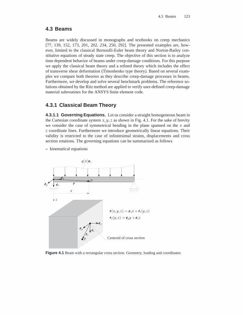
4.3 Beams 123
4.3 Beams
Beams are widely discussed in monographs and textbooks on creep mechanics[77, 139, 152, 173, 201, 202, 234, 250, 292]. The presented examples are, how-ever, limited to the classical Bernoulli-Euler beam theoryand Norton-Bailey con-stitutive equations of steady state creep. The objective ofthis section is to analyzetime dependent behavior of beams under creep-damage conditions. For this purposewe apply the classical beam theory and a refined theory which includes the effectof transverse shear deformation (Timoshenko type theory).Based on several exam-ples we compare both theories as they describe creep-damageprocesses in beams.Furthermore, we develop and solve several benchmark problems. The reference so-lutions obtained by the Ritz method are applied to verify user-defined creep-damagematerial subroutines for the ANSYS finite element code.
4.3.1 Classical Beam Theory
4.3.1.1 Governing Equations. Let us consider a straight homogeneous beam inthe Cartesian coordinate systemx, y, z as shown in Fig. 4.1. For the sake of brevitywe consider the case of symmetrical bending in the plane spanned on thex andz coordinate lines. Furthermore we introduce geometricallylinear equations. Theirvalidity is restricted to the case of infinitesimal strains,displacements and crosssection rotations. The governing equations can be summarized as follows
– kinematical equations
eeex
eeex
eeez
eeez
eeey
eeey
x
q(x)eeez
z
P
Prrr
rrrtCentroid of cross section
rrr(x, y, z) = eeexx + rrrt(y, z)
rrrt(y, z) = eeeyy + eeezz
Figure 4.1 Beam with a rectangular cross section. Geometry, loading and coordinates
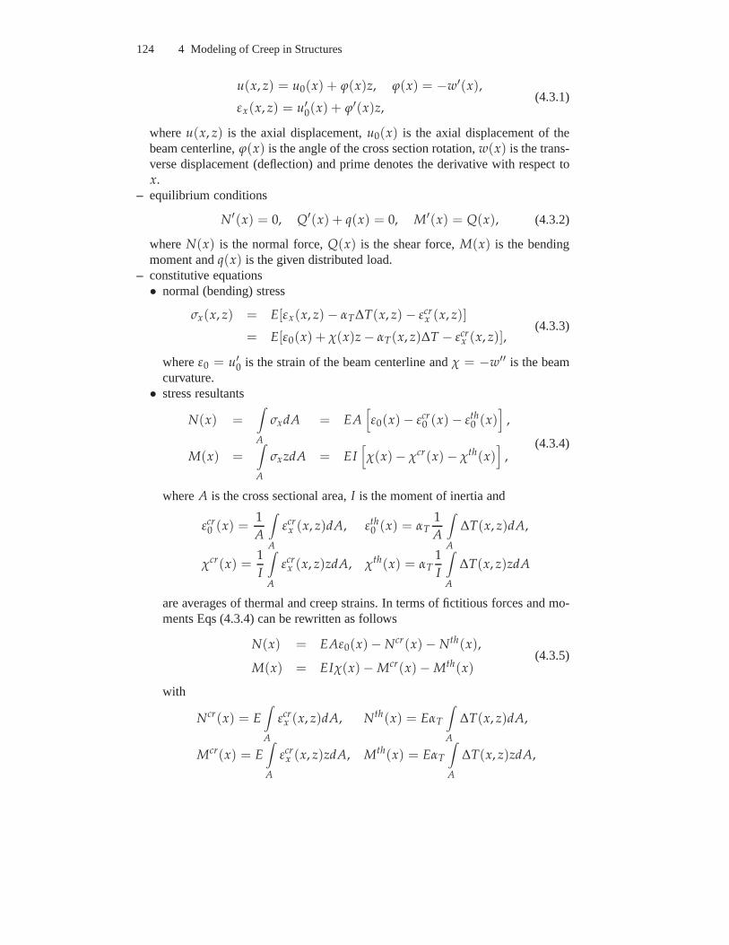
124 4 Modeling of Creep in Structures
u(x, z) = u0(x) + ϕ(x)z, ϕ(x) = −w′(x),
εx(x, z) = u′0(x) + ϕ′(x)z,
(4.3.1)
whereu(x, z) is the axial displacement,u0(x) is the axial displacement of thebeam centerline,ϕ(x) is the angle of the cross section rotation,w(x) is the trans-verse displacement (deflection) and prime denotes the derivative with respect tox.
– equilibrium conditions
N′(x) = 0, Q′(x) + q(x) = 0, M′(x) = Q(x), (4.3.2)
whereN(x) is the normal force,Q(x) is the shear force,M(x) is the bendingmoment andq(x) is the given distributed load.
– constitutive equations• normal (bending) stress
σx(x, z) = E[εx(x, z) − αT∆T(x, z) − εcrx (x, z)]
= E[ε0(x) + χ(x)z − αT(x, z)∆T − εcrx (x, z)],
(4.3.3)
whereε0 = u′0 is the strain of the beam centerline andχ = −w′′ is the beam
curvature.• stress resultants
N(x) =∫
A
σxdA = EA[
ε0(x) − εcr0 (x) − εth
0 (x)]
,
M(x) =∫
A
σxzdA = EI[
χ(x)− χcr(x) − χth(x)]
,(4.3.4)
whereA is the cross sectional area,I is the moment of inertia and
εcr0 (x) =
1
A
∫
A
εcrx (x, z)dA, εth
0 (x) = αT1
A
∫
A
∆T(x, z)dA,
χcr(x) =1
I
∫
A
εcrx (x, z)zdA, χth(x) = αT
1
I
∫
A
∆T(x, z)zdA
are averages of thermal and creep strains. In terms of fictitious forces and mo-ments Eqs (4.3.4) can be rewritten as follows
N(x) = EAε0(x) − Ncr(x) − Nth(x),
M(x) = EIχ(x)− Mcr(x) − Mth(x)(4.3.5)
with
Ncr(x) = E∫
A
εcrx (x, z)dA, Nth(x) = EαT
∫
A
∆T(x, z)dA,
Mcr(x) = E∫
A
εcrx (x, z)zdA, Mth(x) = EαT
∫
A
∆T(x, z)zdA,
4.3 Beams 125
• creep-damage constitutive and evolution equations (see Sect. 2.4.1.1)
εcrx =
a|σx |n−1σx
(1 − ω)n, ω =
bσkeq
(1 − ω)l, σeq = α
|σx | + σx
2+ (1 − α)|σx |
(4.3.6)
The boundary conditions atx = 0 andx = l (l is the beam length) must be formu-lated with respect to the kinematical quantitiesw, ϕ and/or the dual static quantitiesQ, M. The initial conditions att = 0 areεcr
x = 0 andω = 0.
4.3.1.2 Closed Form Solutions. Assuming the idealized creep behavior withthe secondary creep stage only (see Sect. 1.2) a steady stateexists, for which thebending stress and the deflection rate in a beam are constant.Constitutive equationfor secondary creep follows from (4.3.6) by settingb = 0. For the sake of brevitylet us neglect the thermal strains. The constitutive equation for the bending stress(4.3.5) takes the form
σx(x, z) = E [χ(x)z − εcrx (x, z)] (4.3.7)
In the following derivations let us drop the arguments. Taking the time derivative of(4.3.7) and applying the constitutive equation (4.3.6) we obtain
σx = E(χz − a|σx |n−1σx) (4.3.8)
Equation (4.3.8) describes the stress redistribution in a beam. The steady state solu-tion follows from (4.3.8) by settingσx = 0
σx =
(
1
a
) 1n
|χz| 1n −1χz (4.3.9)
The bending moment in the steady state can be calculated as follows
M =∫
A
σxzdA =
(
1
a
) 1n
In|χ|1n −1χ, (4.3.10)
whereIn =
∫
A
|z| 1n−1z2dA
is the generalized moment of inertia.As an example let us consider a simply supported beam under a uniformly dis-
tributed loadq. In this statically determined case the bending moment isM(x) =qx(l − x)/2. From (4.3.10) follows the differential equation for the deflection rate
w(x)′′ = − a
Inn
qn
2nxn(l − x)n, 0 ≤ x ≤ l (4.3.11)
For integer values of the powern the solution is
126 4 Modeling of Creep in Structures
w(x) =a
Inn
qn
2nx
n
∑k=0
αk(ln+k+1 − xn+k+1) (4.3.12)
with
αk = (−1)k n!
k!(n − k)!
ln−k
(n + k + 1)(n + k + 2)
The reference elastic deflection is
w(x) =q
24EIx(x − l)(x2 − lx − l2)
Let us note that the closed form solution for the steady statedeflection rate (4.3.12)is a polynomial of the order2n + 2. Therefore, if the creep problem is numericallysolved applying variational methods (see Sect. 4.2.3.3), the trial functions for the de-flection or deflection rate should contain the polynomial terms of the order2n + 2instead of 4 in the elastic case. The order of the polynomial terms of the creep solu-tion is material-dependent sincen is the creep exponent in the Norton-Bailey creeplaw. Furthermore, for the analysis of steady state creep, anaccurate solution cannotbe obtained applying approximations justified from the elastic solution. Closed formsolutions for steady state creep in beams with various typesof boundary conditionsand loading are presented in [77, 202, 234].
4.3.1.3 Approximate Solutions by the Ritz Method. Starting from the prin-ciple of virtual displacements (4.2.43) we can write
∫
V
σxδεxdV = EI
l∫
0
w′′δw′′dx + EA
l∫
0
u′0δu′
0dx
+
l∫
0
Mcrδw′′dx −l∫
0
Ncrδu′0dx
=
l∫
0
qδwdx
Assuming the creep strain to be known function of the coordinatesx andz for thefixed timet we can formulate the following functional
Πt(w, u0) =1
2EI
l∫
0
w′′2dx +1
2EA
l∫
0
u′20 dx
+
l∫
0
Mcrw′′dx −l∫
0
Ncru′0dx −
l∫
0
qwdx
The problem is to find such functionsw andu0 that yield an extremum of the func-tional. The approximate solutions for the fixed timet can be represented in the formof series
4.3 Beams 127
w(x) = aw0 φw
0 (x) +N
∑i=1
awi φw
i (x), u0(x) =M
∑i=1
aui φu
i (x) (4.3.13)
For the simply supported beam the trial functions can be formulated as follows.φw
0 (x) = x(x− l)(x2 − lx− l2) is the first approximation from the elastic solution.For φw
i (x) we apply the following polynomials satisfying the boundaryconditionsfor the deflectionw = 0 and for the bending momentM = 0 at x = 0 andx = l
φωi (x) = xi+2(l − x)i+2 (4.3.14)
Assuming thatu0 = 0 atx = 0 the functionsφui (x) = xi can be utilized. Collecting
the unknown constant coefficients into the vectoraaaT = [aaawTaaauT
] with aaawT=
[aw0 aw
i ], i = 1, . . . , N andaaauT= [au
i ], i = 1, . . . , M, the Ritz method yields a setof linear algebraic equations
∂Πt
∂ak= 0,
[
RRRww 000000 RRRuu
] [
aaaw
aaau
]
=
[
fff w
fff u
]
(4.3.15)
with
Rwwkj = EI
l∫
0
φwk′′φw
j′′dx, k = 1, . . . , N, j = 1, . . . , N,
Ruukj = EA
l∫
0
φuk′φu
j′dx, k = 1, . . . , M, j = 1, . . . , M,
f wk = q
l∫
0
φwk dx −
l∫
0
Mcrφwk′′dx, k = 1, . . . , N,
f uk =
l∫
0
Ncrφuk′dx, k = 1, . . . , M
After solution of (4.3.15) the stressσx(x, z, t) can be calculated from (4.3.3). Forthe known values of the stress and the damage parameter the constitutive model(4.3.6) yields the rates of creep strain and damage for the time t. From these thenew values for the timet + ∆t are calculated using the implicit time integrationprocedure (4.2.28)
εcr(x, z, t + ∆t) = εcr(x, z, t) + ∆t[(1 − θ)εcr(x, z, t) + θεcr(x, z, t + ∆t)],
ω(x, z, t + ∆t) = ω(x, z, t) + ∆t[(1 − θ)ω(x, z, t) + θω(x, z, t + ∆t)],
εcr(x, z, 0) = 0, ω(x, z, 0) = 0, ω(x, z, t) < ω∗
For the calculation of the fictitious creep forceNcr and the creep momentMcr
the Gauss method with 9 integration points in the thickness direction is used. To
128 4 Modeling of Creep in Structures
obtain the matricesRRRmn(m, n = w, u) and the vectorsfff w and fff u in (4.3.15) theSimpson quadrature rule withNs integration points along the beam length axisx isapplied. The values of creep strain and damage at the currenttime step are storedfor all integration points along the beam axis and over the thickness direction. Theyare used for the calculations at the next time step. The accuracy of the numericalsolution depends on the number of trial functions in Eq. (4.3.13), on the number ofintegration points, and on the time step size.
4.3.1.4 Example. In the following numerical example we examine the conver-gence of the approximate solution by the Ritz method applying different numberof trial functions. Furthermore, we perform the finite element analysis by ANSYScode to verify the developed material subroutine and to illustrate the solution accu-racy with respect to the mesh density.
Solution by the Ritz Method. Let us consider a simply supported and uniformlyloaded beam with a rectangular cross sectiong× h, whereg is the width andh is theheight. For the numerical analysis we setq = 60 N/mm, l = 103 mm,h = 80 mm,ly = 30 mm. We apply the creep-damage material model (3.1.11) with materialconstants for the aluminium alloy BS 1472 (3.1.12) (see Sect. 3.1.4). The damageevolution is controlled by the von Mises equivalent stress.Consequently, the damagerate will be the same for tensile and compressive layers of the beam. By settingα = 0 in (4.3.6) we obtainσeq = |σx |. Therefore, the distribution of|σx | willbe symmetrical with respect to the beam centerline. Furthermore, in Eqs (4.3.15)Ncr = 0, fff u = 000 and consequentlyaaau = 0.
The time step solutions are performed until the critical damage is achieved inone of the integration points. The condition of terminationis ω(x f , z f , t∗) > 0.9,where the integration pointP(x f , z f ) can be specified as a point of failure initia-tion and the time stept∗ as the time to failure initiation. Figure 4.2 illustrates themaximum deflection and the maximum stress as functions of time. The results havebeen obtained with different number of polynomial terms (4.3.14) in Eqs (4.3.13).We observe that all applied approximations to the deflectionfunction provide thesame result for the reference elastic state. However, the results for creep are quitedifferent and depend essentially on the number of trial functions, Fig. 4.2. The ap-proximation adjusted to the elastic solution (fourth orderpolynomial, curves 1) ishardly sufficient for the creep-damage analysis. The difference between the life-timeestimations for the case 1 (N = 1) and for the case 4 (N = 8) is up to the factor six.Figure 4.3 illustrates the convergence against the accurate solution with increasingnumber of trial functions. As shown in Sect. 4.3.1.2, the closed form solution fordeflection rate in the steady state creep range is a polynomial of the order2n + 2,wheren is the material constant in the power law. If the damage evolution is takeninto account then the steady state creep range does not exist, Fig. 4.3. By analogywith the uni-axial creep curve three creep stages for the beam can be observed. The“primary” stage is characterized by the decrease in the deflection rate and signifi-cant stress relaxation. The “secondary” stage can be identified by slow changes inthe rates of deflection growth and stress relaxation. Duringthe “tertiary” stage therates rapidly increase. The applied approximations in the cases 3-6, Fig. 4.3, provide
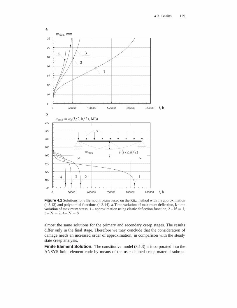
4.3 Beams 129
0 5 0 0 0 0 1 0 0 0 0 0 1 5 0 0 0 0 2 0 0 0 0 0 2 5 0 0 0 08
1 0
1 2
1 4
1 6
1 8
2 0
2 2
0 5 0 0 0 0 1 0 0 0 0 0 1 5 0 0 0 0 2 0 0 0 0 0 2 5 0 0 0 08 0
1 0 0
1 2 0
1 4 0
1 6 0
1 8 0
2 0 0
2 2 0
2 4 0
t, h
t, h
wmax, mm
σmax = σx(l/2, h/2), MPa
1
1
2
2
3
3
4
4
q
lP(l/2, h/2)wmax
a
b
Figure 4.2 Solutions for a Bernoulli beam based on the Ritz method with the approximation(4.3.13) and polynomial functions (4.3.14).a Time variation of maximum deflection,b timevariation of maximum stress, 1 – approximation using elastic deflection function, 2 –N = 1,3 – N = 2, 4 – N = 8
almost the same solutions for the primary and secondary creep stages. The resultsdiffer only in the final stage. Therefore we may conclude thatthe consideration ofdamage needs an increased order of approximation, in comparison with the steadystate creep analysis.
Finite Element Solution. The constitutive model (3.1.3) is incorporated into theANSYS finite element code by means of the user defined creep material subrou-
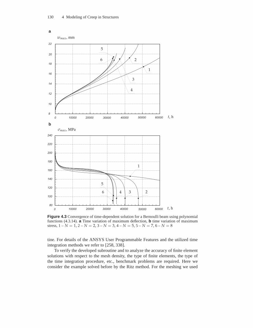
130 4 Modeling of Creep in Structures
0 1 0 0 0 0 2 0 0 0 0 3 0 0 0 0 4 0 0 0 0 5 0 0 0 0 6 0 0 0 08
1 0
1 2
1 4
1 6
1 8
2 0
2 2
0 1 0 0 0 0 2 0 0 0 0 3 0 0 0 0 4 0 0 0 0 5 0 0 0 0 6 0 0 0 08 0
1 0 0
1 2 0
1 4 0
1 6 0
1 8 0
2 0 0
2 2 0
2 4 0
t, h
t, h
wmax, mm
σmax, MPa
1
1
2
2
3
3
4
4
5
5
6
6
a
b
Figure 4.3 Convergence of time-dependent solution for a Bernoulli beam using polynomialfunctions (4.3.14).a Time variation of maximum deflection,b time variation of maximumstress, 1 –N = 1, 2 – N = 2, 3 – N = 3, 4 – N = 5, 5 – N = 7, 6 – N = 8
tine. For details of the ANSYS User Programmable Features and the utilized timeintegration methods we refer to [258, 338].
To verify the developed subroutine and to analyze the accuracy of finite elementsolutions with respect to the mesh density, the type of finiteelements, the type ofthe time integration procedure, etc., benchmark problems are required. Here weconsider the example solved before by the Ritz method. For the meshing we used
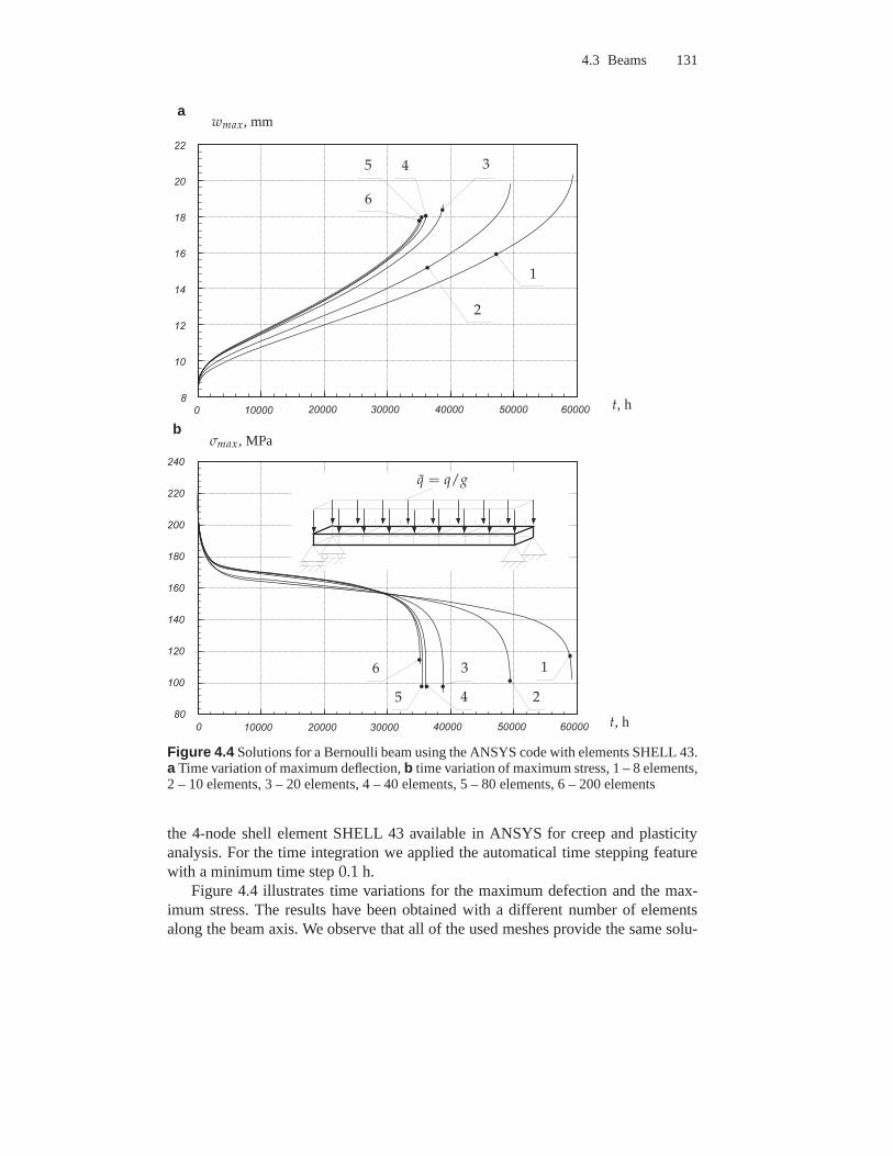
4.3 Beams 131
0 1 0 0 0 0 2 0 0 0 0 3 0 0 0 0 4 0 0 0 0 5 0 0 0 0 6 0 0 0 08
1 0
1 2
1 4
1 6
1 8
2 0
2 2
0 1 0 0 0 0 2 0 0 0 0 3 0 0 0 0 4 0 0 0 0 5 0 0 0 0 6 0 0 0 08 0
1 0 0
1 2 0
1 4 0
1 6 0
1 8 0
2 0 0
2 2 0
2 4 0
t, h
t, h
wmax, mm
σmax, MPa
1
1
2
2
3
3
4
4
5
5
6
6
q = q/g
a
b
Figure 4.4 Solutions for a Bernoulli beam using the ANSYS code with elements SHELL 43.a Time variation of maximum deflection,b time variation of maximum stress, 1 – 8 elements,2 – 10 elements, 3 – 20 elements, 4 – 40 elements, 5 – 80 elements, 6 – 200 elements
the 4-node shell element SHELL 43 available in ANSYS for creep and plasticityanalysis. For the time integration we applied the automatical time stepping featurewith a minimum time step0.1 h.
Figure 4.4 illustrates time variations for the maximum defection and the max-imum stress. The results have been obtained with a differentnumber of elementsalong the beam axis. We observe that all of the used meshes provide the same solu-
132 4 Modeling of Creep in Structures
tions for the reference elastic state. However, the creep solutions are highly sensitiveto the mesh density. The best solution (case 6) has been obtained with 200 elementsand after 96 time steps. This solution agrees well with the solution obtained by theRitz method, Fig. 4.3. A mesh adjusted to the convergent solution of the linear elas-ticity problem (case 1) is not fine enough for the creep analysis. The results in thecases 3-6, Fig. 4.4 agree well in the primary and secondary creep stages and dif-fer only in the final stage. However, such a difference is not essential if we takeinto account the scatter of material data and inaccuracy of the material behavior de-scription. In this sence the mesh adjusted to the convergentsolution in the pimaryand secondary creep stages is fine enough for the numerical life-time predictions.In [14, 15] several benchmark problems for beams and rectangular plates solved bythe Ritz method are presented. Finite element solutions forthe same problems havebeen perfomed by use of shell, plane and solid type elements.The results illustratethe correctness of the developed subroutine over the wide range of element types.Furthermore, the conclusion was made, that the mesh adjusted to convergent solu-tions in the primary and secondary creep range provides enough accuracy for theanalysis of the whole creep process.
4.3.2 Refined Theories of Beams
4.3.2.1 Stress State Effects and Cross Section Assumptions . For manymaterials stress state dependent tertiary creep has been observed in multi-axial tests(see Sect. 1.1.2). The primary and secondary creep rates aredominantly controlledby the von Mises stress. The accelerated creep is additionally influenced by the kindof the stress state. For example, different tertiary creep rates and times to fracturecan be obtained from creep tests under uni-axial tension with the stressσ and undertorsion with the shear stress
√3τ = σ, e.g. [169]. Figure 4.5a shows creep curves
for tensile, compressive and shearing stresses simulated according to the constitutivemodel (3.1.1), (3.1.2) and the material constants (3.1.3) for type 316 stainless steelat 650 C. The selected stress values provide the same value of the von Mises stress.It is obvious that the tertiary creep rate is significantly dependent on the kind ofloading. Figure 4.5b presents creep curves calculated by the combined action of thenormal and shear stresses. We observe that even a small superposed shear stress cansignificantly influence the axial strain response and decrease the fracture time. Fur-thermore, combined tension-shear and compression-shear loadings with the samestress magnitudes lead to quite different creep responses.The change of the sign ofthe normal stress influences both the normal and the shear creep rates.
The considered loading case is typical for transversely loaded beams, plates andshells. For beams the local stress state is characterized bynormal (bending) stressand small superposed transverse shear stress. Transverse shear stress and transverseshear deformation are neglected within the classical theory of beams. The consid-ered example indicates that small shear stress can significantly influence the ma-terial response and cause significant shear strains. Furthermore, the dependence ofcreep on the sign of the normal stress can lead to non-classical thickness distribu-tions of the displacement, strain and stress fields. For example, the concept of the
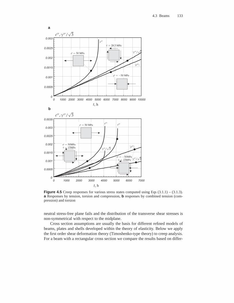
4.3 Beams 133
0 1 0 0 0 2 0 0 0 3 0 0 0 4 0 0 0 5 0 0 0 6 0 0 0 7 0 0 0 8 0 0 0 9 0 0 0 1 0 0 0 00
0 . 0 0 0 5
0 . 0 0 1
0 . 0 0 1 5
0 . 0 0 2
0 . 0 0 2 5
0 . 0 0 3
0 1 0 0 0 2 0 0 0 3 0 0 0 4 0 0 0 5 0 0 0 6 0 0 0 7 0 0 00
0 . 0 0 0 5
0 . 0 0 1
0 . 0 0 1 5
0 . 0 0 2
0 . 0 0 2 5
0 . 0 0 3
0 . 0 0 3 5
t, h
t, h
εcr, γcr/√
3
εcr, γcr/√
3
σ = 50 MPa
τ = 28.5 MPa
σ = −50 MPa
σ = 50MPaτ = 15MPa
σ = 50 MPa
σ = −50MPaτ = 15MPa
εcrεcr
εcr
γcr/√
3
γcr/√
3
γcr/√
3
|εcr|
|εcr|
a
b
Figure 4.5 Creep responses for various stress states computed using Eqs (3.1.1) – (3.1.3).a Responses by tension, torsion and compression,b responses by combined tension (com-pression) and torsion
neutral stress-free plane fails and the distribution of thetransverse shear stresses isnon-symmetrical with respect to the midplane.
Cross section assumptions are usually the basis for different refined models ofbeams, plates and shells developed within the theory of elasticity. Below we applythe first order shear deformation theory (Timoshenko-type theory) to creep analysis.For a beam with a rectangular cross section we compare the results based on differ-
134 4 Modeling of Creep in Structures
ent structural mechanics models (classical beam, shear deformable beam and planestress model).
4.3.2.2 First Order Shear Deformation Equations. The first order shear de-formation beam theory can be derived either by the direct approach, e.g. [32], or bya variational method applied to three-dimensional equations, e.g. [20, 140].
Within the direct approach the beam is modeled as a deformable oriented line.The deformed configuration is characterized by two independent kinematical quan-tities: the vector describing the positions of points on theline and the rotation tensoror vector describing the orientation of cross sections. Furthermore, it is assumed thatthe mechanical interaction between neighboring cross sections is only due to forcesand moments. The balance equations are applied directly to the deformable lineand formulated with respect to the beam quantities, i.e. theline mass density (massdensity per unit arc length), the vectors of forces and moments, the line densityof internal energy, etc. The constitutive equations connect the forces and momentswith the strains. A direct approach to formulate constitutive equations for rods andshells in the case of elasticity is discussed in [23]. Despite the elegance of this ap-proach several problems arise in application to creep mechanics. The creep consti-tutive equations must be formulated for inelastic parts of beam like strains (tensile,transverse shear and bending strains). By analogy to the creep theories discussed inChapt. 2 the creep potential should be constructed as a function of the force and themoment vectors. For example, letTTT be the force vector andMMM the moment vector.Following the classical creep theory (see Sect. 2.2.1.1) anequivalent stress for thedeformable line can be formulated as a quadratic form with respect toTTT andMMM
t2eq =
1
2TTT ··· AAA ··· TTT + TTT ··· BBB ··· MMM +
1
2MMM ···CCC ··· MMM
The structure of second rank material tensorsAAA, BBB andCCC must be established ac-cording to the material symmetries and geometrical symmetries of the beam crosssection. The material constants have to be identified eitherfrom creep tests on beamsor by comparing the solutions of beam equations with the corresponding solutionsof three- or two-dimensional problems for special cases of loading. Only a few suchsolutions are available in creep mechanics. An example is the pure bending of abeam under power law secondary creep condition (see Sect. 4.3.1.2). In this casethe steady state creep constitutive equation for the bending strain rate can be ob-tained from (4.3.10) as follows
χ =a
Inn|M|n−1 M
Alternatively the beam equations may be derived in the senseof approximate so-lution of two- or three-dimensional equations. First, through-the-thickness approx-imations of displacements and/or stresses are specified. Then, the two- or three-dimensional boundary value problem is reduced to ordinary differential equationsby means of a variational principle. In order to discuss thisapproach let us considera beam with a rectangular cross-section, Fig. 4.6. The governing two-dimensional
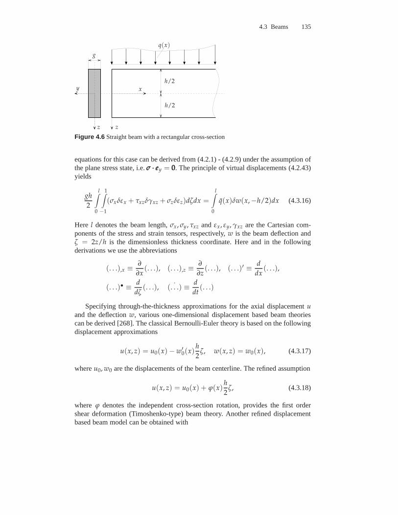
4.3 Beams 135
x
z z
y
h/2
h/2
g
q(x)
Figure 4.6 Straight beam with a rectangular cross-section
equations for this case can be derived from (4.2.1) - (4.2.9)under the assumption ofthe plane stress state, i.e.σσσ ··· eeey = 000. The principle of virtual displacements (4.2.43)yields
gh
2
l∫
0
1∫
−1
(σxδεx + τxzδγxz + σzδεz)dζdx =
l∫
0
q(x)δw(x,−h/2)dx (4.3.16)
Here l denotes the beam length,σx, σy, τxz and εx, εy, γxz are the Cartesian com-ponents of the stress and strain tensors, respectively,w is the beam deflection andζ = 2z/h is the dimensionless thickness coordinate. Here and in the followingderivations we use the abbreviations
(. . .),x ≡ ∂
∂x(. . .), (. . .),z ≡
∂
∂z(. . .), (. . .)′ ≡ d
dx(. . .),
(. . .)• ≡ d
dζ(. . .), ˙(. . .) ≡ d
dt(. . .)
Specifying through-the-thickness approximations for theaxial displacementuand the deflectionw, various one-dimensional displacement based beam theoriescan be derived [268]. The classical Bernoulli-Euler theoryis based on the followingdisplacement approximations
u(x, z) = u0(x) − w′0(x)
h
2ζ, w(x, z) = w0(x), (4.3.17)
whereu0, w0 are the displacements of the beam centerline. The refined assumption
u(x, z) = u0(x) + ϕ(x)h
2ζ, (4.3.18)
where ϕ denotes the independent cross-section rotation, providesthe first ordershear deformation (Timoshenko-type) beam theory. Anotherrefined displacementbased beam model can be obtained with
136 4 Modeling of Creep in Structures
u(x, ζ) = u0(x) + ϕ(x)h
2ζ + u1(x)Φ(ζ),
w(x, ζ) = w0(x) + w1(x)Ω(ζ),(4.3.19)
whereu0 and w0 are the displacements of the beam centerline,Φ(ζ) and Ω(ζ)are distribution functions, which should be specified, andu1(x) andw1(x) are un-known functions of thex-coordinate. The assumptionsΦ(ζ) = (ζh/2)3 , Ω(z) = 0result in a Levinson-Reddy type theory [186, 267]. From the boundary conditionsγxz(x,±1) = 0 it follows
u(x, ζ) = u0(x) + ϕ(x)h
2ζ − [w′
0(x) + ϕ(x)]h
6ζ3,
w(x, ζ) = w0(x)
anddΦ
dζ
∣
∣
∣
ζ=−1=
dΦ
dζ
∣
∣
∣
ζ=1
The next possibility is the use of stress based approximations. For example,the equations following from the elasticity solution of theBernoulli-Euler beamequations are given as
σx =6M(x)
gh2ζ,
τxz =3Q(x)
2gh
(
1 − ζ2)
,
σz =3q(x)
4g
(
−2
3+ ζ − 1
3ζ3
)
(4.3.20)
Applying the stress approximations equations for an elastic shear deformable platehave been derived by E. Reissner [270] by means of a mixed variational principle.The displacement approximations (4.3.19) neglecting the termsu1Φ andw1Ω orthe stress approximations (4.3.20) lead to the first order shear deformation beamtheory. The stress approximations (4.3.20) are not suitable for creep problems be-cause even in the case of steady state creep the normal stressσx is a non-linearfunction of the thickness coordinate (see Sect. 4.3.1.2). To avoid this problem, in[20] the following approximations for the transverse shearand normal stresses wereapplied
τxz =2Q(x)
gh
ψ•(ζ)
ψ0,
σz =q(x)
g
ψ(ζ) − ψ(1)
ψ0, ψ0 = ψ(1) − ψ(−1)
(4.3.21)
ψ(ζ) is a given function satisfying the boundary conditionsψ•(±1) = 0. Fur-thermore, the linear through-the-thickness approximation of the axial displacementu(x, ζ) = u0(x) + ζϕ(x)h/2 was assumed. Applying a mixed type variationalprinciple the following beam equations were derived in [20]
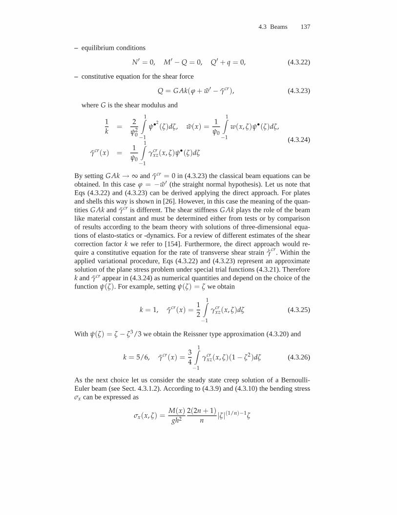
4.3 Beams 137
– equilibrium conditions
N′ = 0, M′ − Q = 0, Q′ + q = 0, (4.3.22)
– constitutive equation for the shear force
Q = GAk(ϕ + w′ − γcr), (4.3.23)
whereG is the shear modulus and
1
k=
2
ψ20
1∫
−1
ψ•2(ζ)dζ, w(x) =
1
ψ0
1∫
−1
w(x, ζ)ψ•(ζ)dζ,
γcr(x) =1
ψ0
1∫
−1
γcrxz(x, ζ)ψ•(ζ)dζ
(4.3.24)
By settingGAk → ∞ andγcr = 0 in (4.3.23) the classical beam equations can beobtained. In this caseϕ = −w′ (the straight normal hypothesis). Let us note thatEqs (4.3.22) and (4.3.23) can be derived applying the directapproach. For platesand shells this way is shown in [26]. However, in this case themeaning of the quan-tities GAk andγcr is different. The shear stiffnessGAk plays the role of the beamlike material constant and must be determined either from tests or by comparisonof results according to the beam theory with solutions of three-dimensional equa-tions of elasto-statics or -dynamics. For a review of different estimates of the shearcorrection factork we refer to [154]. Furthermore, the direct approach would re-quire a constitutive equation for the rate of transverse shear strain ˙γ
cr. Within theapplied variational procedure, Eqs (4.3.22) and (4.3.23) represent an approximatesolution of the plane stress problem under special trial functions (4.3.21). Thereforek andγcr appear in (4.3.24) as numerical quantities and depend on thechoice of thefunctionψ(ζ). For example, settingψ(ζ) = ζ we obtain
k = 1, γcr(x) =1
2
1∫
−1
γcrxz(x, ζ)dζ (4.3.25)
With ψ(ζ) = ζ − ζ3/3 we obtain the Reissner type approximation (4.3.20) and
k = 5/6, γcr(x) =3
4
1∫
−1
γcrxz(x, ζ)(1 − ζ2)dζ (4.3.26)
As the next choice let us consider the steady state creep solution of a Bernoulli-Euler beam (see Sect. 4.3.1.2). According to (4.3.9) and (4.3.10) the bending stressσx can be expressed as
σx(x, ζ) =M(x)
gh2
2(2n + 1)
n|ζ|(1/n)−1ζ
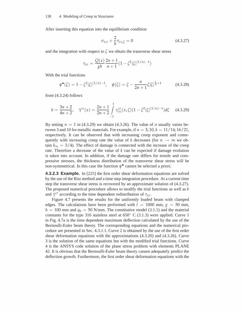
138 4 Modeling of Creep in Structures
After inserting this equation into the equilibrium condition
σx,x +2
hτxz,ζ = 0 (4.3.27)
and the integration with respect toζ we obtain the transverse shear stress
τxz =Q(x)
gh
2n + 1
n + 1(1 − ζ2|ζ|(1/n)−1)
With the trial functions
ψ•(ζ) = 1 − ζ2|ζ|(1/n)−1, ψ(ζ) = ζ − n
2n + 1ζ|ζ| 1
n +1 (4.3.28)
from (4.3.24) follows
k =3n + 2
4n + 2, γcr(x) =
2n + 1
2n + 2
1∫
−1
γcrxz(x, ζ)(1 − ζ2|ζ|(1/n)−1)dζ (4.3.29)
By settingn = 1 in (4.3.29) we obtain (4.3.26). The value ofn usually varies be-tween 3 and 10 for metallic materials. For example, ifn = 3; 10, k = 11/14; 16/21,respectively. It can be observed that with increasing creepexponent and conse-quently with increasing creep rate the value ofk decreases (forn → ∞ we ob-tain k∞ = 3/4). The effect of damage is connected with the increase of the creeprate. Therefore a decrease of the value ofk can be expected if damage evolutionis taken into account. In addition, if the damage rate differs for tensile and com-pressive stresses, the thickness distribution of the transverse shear stress will benon-symmetrical. In this case the functionψ• cannot be selected a priori.
4.3.2.3 Example. In [225] the first order shear deformation equations are solvedby the use of the Ritz method and a time step integration procedure. At a current timestep the transverse shear stress is recovered by an approximate solution of (4.3.27).The proposed numerical procedure allows to modify the trialfunctions as well askandγcr according to the time dependent redistribution ofτxz.
Figure 4.7 presents the results for the uniformly loaded beam with clampededges. The calculations have been performed withl = 1000 mm, g = 50 mm,h = 100 mm andq0 = 50 N/mm. The constitutive model (3.1.1) and the materialconstants for the type 316 stainless steel at 650 C (3.1.3) were applied. Curve 1in Fig. 4.7a is the time dependent maximum deflection calculated by the use of theBernoulli-Euler beam theory. The corresponding equationsand the numerical pro-cedure are presented in Sec. 4.3.1.1. Curve 2 is obtained by the use of the first ordershear deformation equations with the approximations (4.3.20) and (4.3.26). Curve3 is the solution of the same equations but with the modified trial functions. Curve4 is the ANSYS code solution of the plane stress problem with elements PLANE42. It is obvious that the Bernoulli-Euler beam theory cannot adequately predict thedeflection growth. Furthermore, the first order shear deformation equations with the
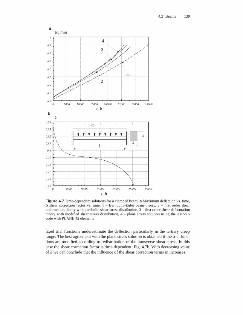
4.3 Beams 139
0 5 0 0 0 1 0 0 0 0 1 5 0 0 0 2 0 0 0 0 2 5 0 0 0 3 0 0 0 0 3 5 0 0 00 . 2
0 . 3
0 . 4
0 . 5
0 . 6
0 . 7
0 . 8
0 . 9
1
0 5 0 0 0 1 0 0 0 0 1 5 0 0 0 2 0 0 0 0 2 5 0 0 0 3 0 0 0 00 . 7 5
0 . 7 6
0 . 7 7
0 . 7 8
0 . 7 9
0 . 8
0 . 8 1
0 . 8 2
0 . 8 3
0 . 8 4
t, h
t, h
w, mm
k
1
2
3
4
l
q0
g
h
a
b
Figure 4.7 Time-dependent solutions for a clamped beam.a Maximum deflection vs. time,b shear correction factor vs. time, 1 – Bernoulli–Euler beam theory, 2 – first order sheardeformation theory with parabolic shear stress distribution, 3 – first order shear deformationtheory with modified shear stress distribution, 4 – plane stress solution using the ANSYScode with PLANE 42 elements
fixed trial functions underestimate the deflection particularly in the tertiary creeprange. The best agreement with the plane stress solution is obtained if the trial func-tions are modified according to redistribution of the transverse shear stress. In thiscase the shear correction factor is time-dependent, Fig. 4.7b. With decreasing valueof k we can conclude that the influence of the shear correction terms in increases.
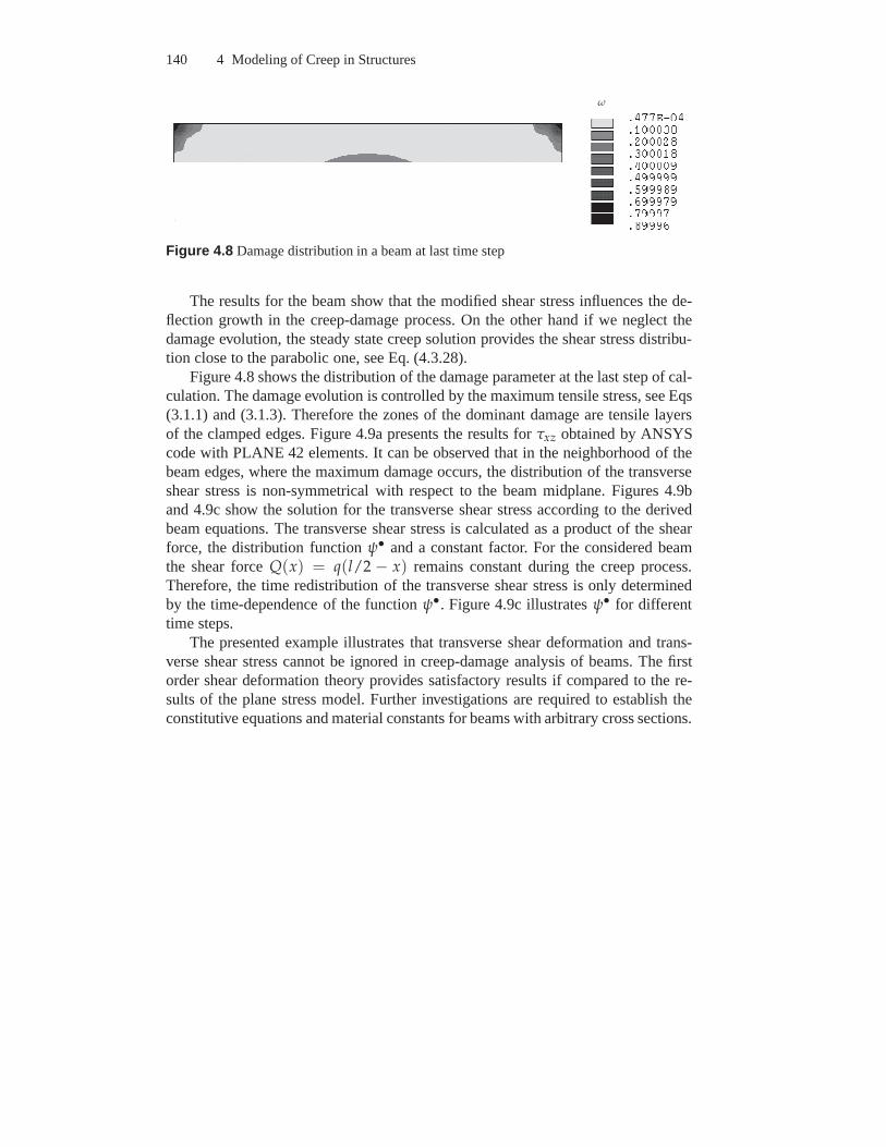
140 4 Modeling of Creep in Structures
ω
Figure 4.8 Damage distribution in a beam at last time step
The results for the beam show that the modified shear stress influences the de-flection growth in the creep-damage process. On the other hand if we neglect thedamage evolution, the steady state creep solution providesthe shear stress distribu-tion close to the parabolic one, see Eq. (4.3.28).
Figure 4.8 shows the distribution of the damage parameter atthe last step of cal-culation. The damage evolution is controlled by the maximumtensile stress, see Eqs(3.1.1) and (3.1.3). Therefore the zones of the dominant damage are tensile layersof the clamped edges. Figure 4.9a presents the results forτxz obtained by ANSYScode with PLANE 42 elements. It can be observed that in the neighborhood of thebeam edges, where the maximum damage occurs, the distribution of the transverseshear stress is non-symmetrical with respect to the beam midplane. Figures 4.9band 4.9c show the solution for the transverse shear stress according to the derivedbeam equations. The transverse shear stress is calculated as a product of the shearforce, the distribution functionψ• and a constant factor. For the considered beamthe shear forceQ(x) = q(l/2 − x) remains constant during the creep process.Therefore, the time redistribution of the transverse shearstress is only determinedby the time-dependence of the functionψ•. Figure 4.9c illustratesψ• for differenttime steps.
The presented example illustrates that transverse shear deformation and trans-verse shear stress cannot be ignored in creep-damage analysis of beams. The firstorder shear deformation theory provides satisfactory results if compared to the re-sults of the plane stress model. Further investigations arerequired to establish theconstitutive equations and material constants for beams with arbitrary cross sections.
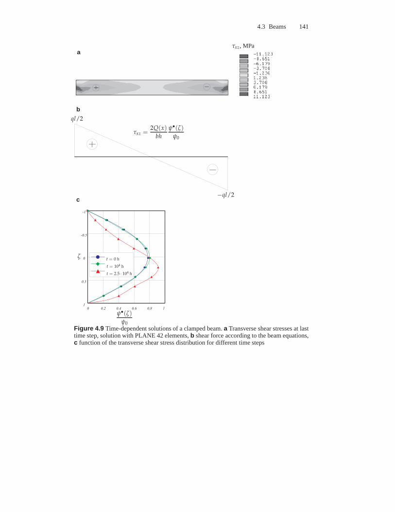
4.3 Beams 141
- 1
- 0 . 5
0
0 . 5
10 0 . 2 0 . 4 0 . 6 0 . 8 1
ql/2
−ql/2
ζ
ψ•(ζ)
ψ0
t = 0 h
t = 104 h
τxz, MPa
t = 2.5 · 104 h
τxz =2Q(x)
bh
ψ•(ζ)
ψ0
a
b
c
Figure 4.9 Time-dependent solutions of a clamped beam.a Transverse shear stresses at lasttime step, solution with PLANE 42 elements,b shear force according to the beam equations,c function of the transverse shear stress distribution for different time steps
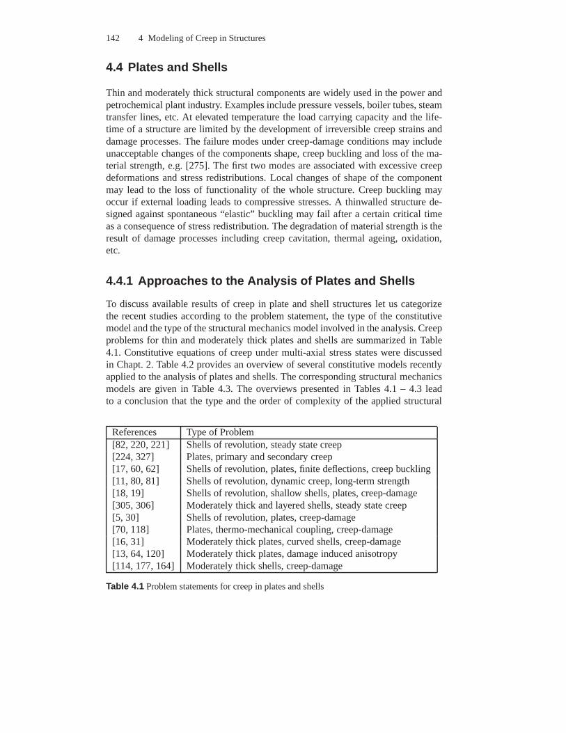
142 4 Modeling of Creep in Structures
4.4 Plates and Shells
Thin and moderately thick structural components are widelyused in the power andpetrochemical plant industry. Examples include pressure vessels, boiler tubes, steamtransfer lines, etc. At elevated temperature the load carrying capacity and the life-time of a structure are limited by the development of irreversible creep strains anddamage processes. The failure modes under creep-damage conditions may includeunacceptable changes of the components shape, creep buckling and loss of the ma-terial strength, e.g. [275]. The first two modes are associated with excessive creepdeformations and stress redistributions. Local changes ofshape of the componentmay lead to the loss of functionality of the whole structure.Creep buckling mayoccur if external loading leads to compressive stresses. A thinwalled structure de-signed against spontaneous “elastic” buckling may fail after a certain critical timeas a consequence of stress redistribution. The degradationof material strength is theresult of damage processes including creep cavitation, thermal ageing, oxidation,etc.
4.4.1 Approaches to the Analysis of Plates and Shells
To discuss available results of creep in plate and shell structures let us categorizethe recent studies according to the problem statement, the type of the constitutivemodel and the type of the structural mechanics model involved in the analysis. Creepproblems for thin and moderately thick plates and shells aresummarized in Table4.1. Constitutive equations of creep under multi-axial stress states were discussedin Chapt. 2. Table 4.2 provides an overview of several constitutive models recentlyapplied to the analysis of plates and shells. The corresponding structural mechanicsmodels are given in Table 4.3. The overviews presented in Tables 4.1 – 4.3 leadto a conclusion that the type and the order of complexity of the applied structural
References Type of Problem[82, 220, 221] Shells of revolution, steady state creep[224, 327] Plates, primary and secondary creep[17, 60, 62] Shells of revolution, plates, finite deflections, creep buckling[11, 80, 81] Shells of revolution, dynamic creep, long-term strength[18, 19] Shells of revolution, shallow shells, plates, creep-damage[305, 306] Moderately thick and layered shells, steady state creep[5, 30] Shells of revolution, plates, creep-damage[70, 118] Plates, thermo-mechanical coupling, creep-damage[16, 31] Moderately thick plates, curved shells, creep-damage[13, 64, 120] Moderately thick plates, damage induced anisotropy[114, 177, 164] Moderately thick shells, creep-damage
Table 4.1 Problem statements for creep in plates and shells
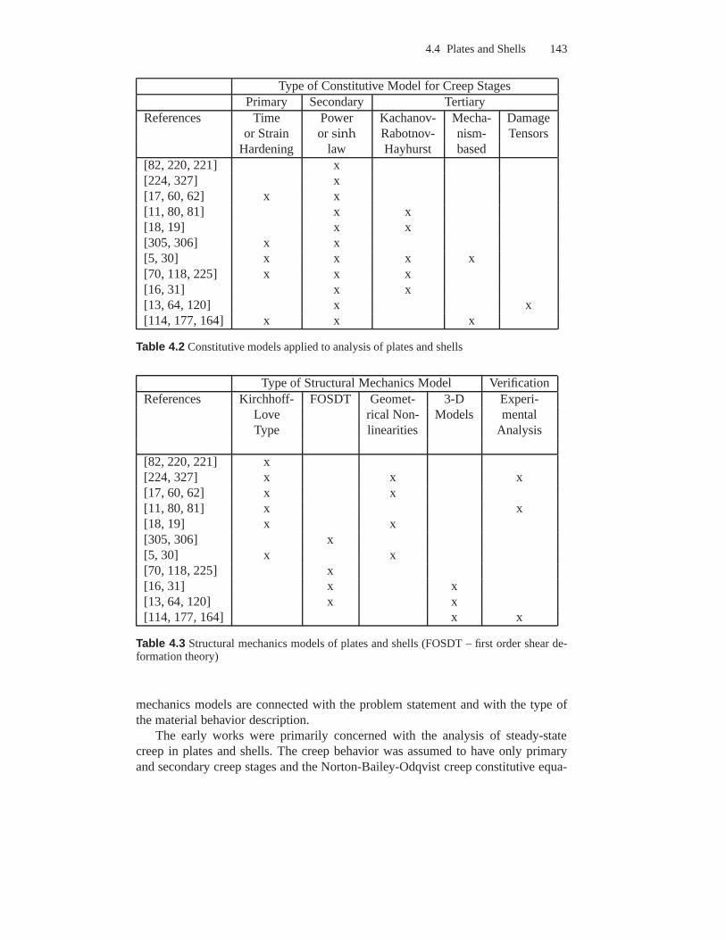
4.4 Plates and Shells 143
Type of Constitutive Model for Creep StagesPrimary Secondary Tertiary
References Time Power Kachanov- Mecha- Damageor Strain or sinh Rabotnov- nism- Tensors
Hardening law Hayhurst based[82, 220, 221] x[224, 327] x[17, 60, 62] x x[11, 80, 81] x x[18, 19] x x[305, 306] x x[5, 30] x x x x[70, 118, 225] x x x[16, 31] x x[13, 64, 120] x x[114, 177, 164] x x x
Table 4.2 Constitutive models applied to analysis of plates and shells
Type of Structural Mechanics Model VerificationReferences Kirchhoff- FOSDT Geomet- 3-D Experi-
Love rical Non- Models mentalType linearities Analysis
[82, 220, 221] x[224, 327] x x x[17, 60, 62] x x[11, 80, 81] x x[18, 19] x x[305, 306] x[5, 30] x x[70, 118, 225] x[16, 31] x x[13, 64, 120] x x[114, 177, 164] x x
Table 4.3 Structural mechanics models of plates and shells (FOSDT – first order shear de-formation theory)
mechanics models are connected with the problem statement and with the type ofthe material behavior description.
The early works were primarily concerned with the analysis of steady-statecreep in plates and shells. The creep behavior was assumed tohave only primaryand secondary creep stages and the Norton-Bailey-Odqvist creep constitutive equa-
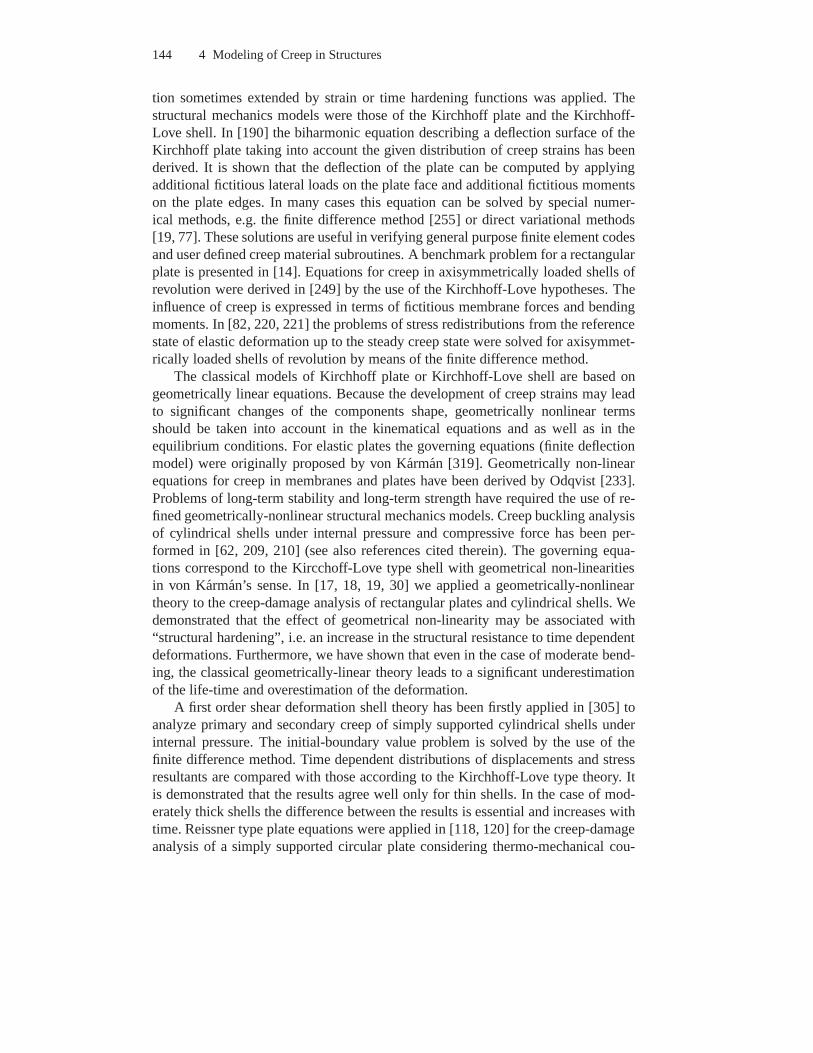
144 4 Modeling of Creep in Structures
tion sometimes extended by strain or time hardening functions was applied. Thestructural mechanics models were those of the Kirchhoff plate and the Kirchhoff-Love shell. In [190] the biharmonic equation describing a deflection surface of theKirchhoff plate taking into account the given distributionof creep strains has beenderived. It is shown that the deflection of the plate can be computed by applyingadditional fictitious lateral loads on the plate face and additional fictitious momentson the plate edges. In many cases this equation can be solved by special numer-ical methods, e.g. the finite difference method [255] or direct variational methods[19, 77]. These solutions are useful in verifying general purpose finite element codesand user defined creep material subroutines. A benchmark problem for a rectangularplate is presented in [14]. Equations for creep in axisymmetrically loaded shells ofrevolution were derived in [249] by the use of the Kirchhoff-Love hypotheses. Theinfluence of creep is expressed in terms of fictitious membrane forces and bendingmoments. In [82, 220, 221] the problems of stress redistributions from the referencestate of elastic deformation up to the steady creep state were solved for axisymmet-rically loaded shells of revolution by means of the finite difference method.
The classical models of Kirchhoff plate or Kirchhoff-Love shell are based ongeometrically linear equations. Because the development of creep strains may leadto significant changes of the components shape, geometrically nonlinear termsshould be taken into account in the kinematical equations and as well as in theequilibrium conditions. For elastic plates the governing equations (finite deflectionmodel) were originally proposed by von Karman [319]. Geometrically non-linearequations for creep in membranes and plates have been derived by Odqvist [233].Problems of long-term stability and long-term strength have required the use of re-fined geometrically-nonlinear structural mechanics models. Creep buckling analysisof cylindrical shells under internal pressure and compressive force has been per-formed in [62, 209, 210] (see also references cited therein). The governing equa-tions correspond to the Kircchoff-Love type shell with geometrical non-linearitiesin von Karman’s sense. In [17, 18, 19, 30] we applied a geometrically-nonlineartheory to the creep-damage analysis of rectangular plates and cylindrical shells. Wedemonstrated that the effect of geometrical non-linearitymay be associated with“structural hardening”, i.e. an increase in the structuralresistance to time dependentdeformations. Furthermore, we have shown that even in the case of moderate bend-ing, the classical geometrically-linear theory leads to a significant underestimationof the life-time and overestimation of the deformation.
A first order shear deformation shell theory has been firstly applied in [305] toanalyze primary and secondary creep of simply supported cylindrical shells underinternal pressure. The initial-boundary value problem is solved by the use of thefinite difference method. Time dependent distributions of displacements and stressresultants are compared with those according to the Kirchhoff-Love type theory. Itis demonstrated that the results agree well only for thin shells. In the case of mod-erately thick shells the difference between the results is essential and increases withtime. Reissner type plate equations were applied in [118, 120] for the creep-damageanalysis of a simply supported circular plate considering thermo-mechanical cou-
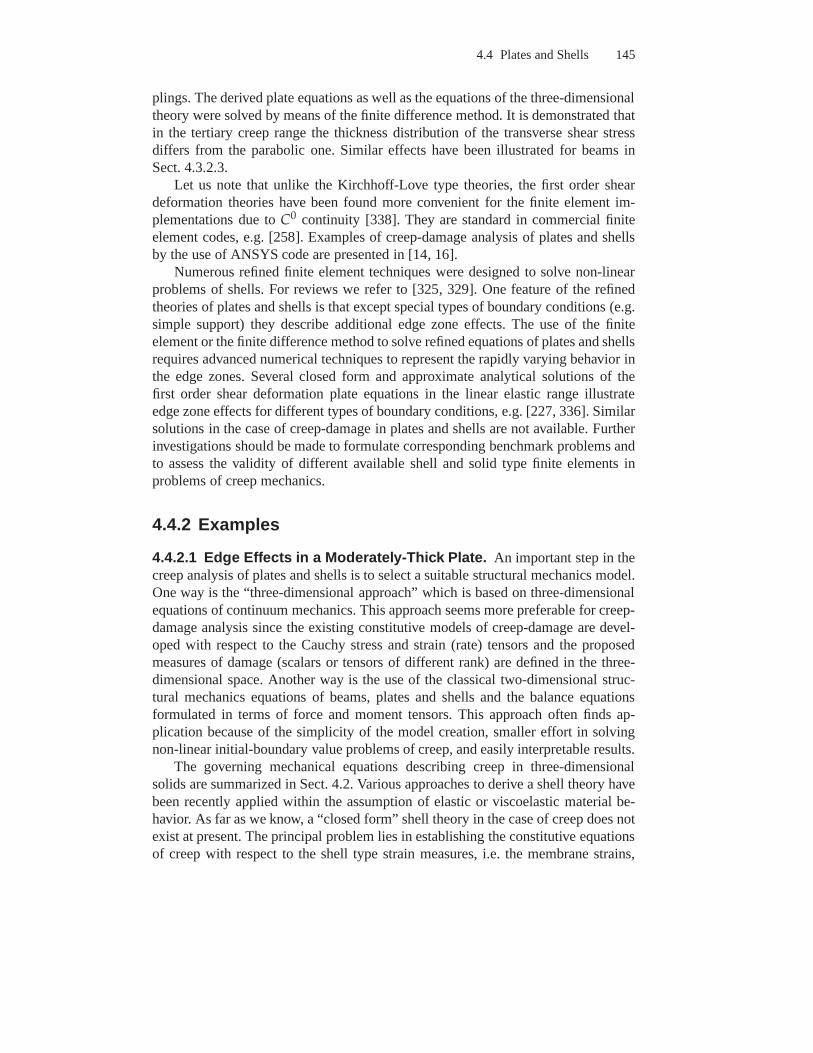
4.4 Plates and Shells 145
plings. The derived plate equations as well as the equationsof the three-dimensionaltheory were solved by means of the finite difference method. It is demonstrated thatin the tertiary creep range the thickness distribution of the transverse shear stressdiffers from the parabolic one. Similar effects have been illustrated for beams inSect. 4.3.2.3.
Let us note that unlike the Kirchhoff-Love type theories, the first order sheardeformation theories have been found more convenient for the finite element im-plementations due toC0 continuity [338]. They are standard in commercial finiteelement codes, e.g. [258]. Examples of creep-damage analysis of plates and shellsby the use of ANSYS code are presented in [14, 16].
Numerous refined finite element techniques were designed to solve non-linearproblems of shells. For reviews we refer to [325, 329]. One feature of the refinedtheories of plates and shells is that except special types ofboundary conditions (e.g.simple support) they describe additional edge zone effects. The use of the finiteelement or the finite difference method to solve refined equations of plates and shellsrequires advanced numerical techniques to represent the rapidly varying behavior inthe edge zones. Several closed form and approximate analytical solutions of thefirst order shear deformation plate equations in the linear elastic range illustrateedge zone effects for different types of boundary conditions, e.g. [227, 336]. Similarsolutions in the case of creep-damage in plates and shells are not available. Furtherinvestigations should be made to formulate corresponding benchmark problems andto assess the validity of different available shell and solid type finite elements inproblems of creep mechanics.
4.4.2 Examples
4.4.2.1 Edge Effects in a Moderately-Thick Plate. An important step in thecreep analysis of plates and shells is to select a suitable structural mechanics model.One way is the “three-dimensional approach” which is based on three-dimensionalequations of continuum mechanics. This approach seems morepreferable for creep-damage analysis since the existing constitutive models of creep-damage are devel-oped with respect to the Cauchy stress and strain (rate) tensors and the proposedmeasures of damage (scalars or tensors of different rank) are defined in the three-dimensional space. Another way is the use of the classical two-dimensional struc-tural mechanics equations of beams, plates and shells and the balance equationsformulated in terms of force and moment tensors. This approach often finds ap-plication because of the simplicity of the model creation, smaller effort in solvingnon-linear initial-boundary value problems of creep, and easily interpretable results.
The governing mechanical equations describing creep in three-dimensionalsolids are summarized in Sect. 4.2. Various approaches to derive a shell theory havebeen recently applied within the assumption of elastic or viscoelastic material be-havior. As far as we know, a “closed form” shell theory in the case of creep does notexist at present. The principal problem lies in establishing the constitutive equationsof creep with respect to the shell type strain measures, i.e.the membrane strains,
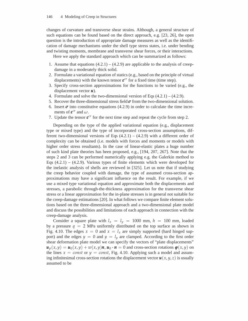
146 4 Modeling of Creep in Structures
changes of curvature and transverse shear strains. Although, a general structure ofsuch equations can be found based on the direct approach, e.g. [23, 26], the openquestion is the introduction of appropriate damage measures as well as the identifi-cation of damage mechanisms under the shell type stress states, i.e. under bendingand twisting moments, membrane and transverse shear forces, or their interactions.
Here we apply the standard approach which can be summarized as follows:
1. Assume that equations (4.2.1) – (4.2.9) are applicable tothe analysis of creep-damage in a moderately thick solid.
2. Formulate a variational equation of statics (e.g., basedon the principle of virtualdisplacements) with the known tensorεεεcr for a fixed time (time step).
3. Specify cross-section approximations for the functionsto be varied (e.g., thedisplacement vectoruuu).
4. Formulate and solve the two-dimensional version of Eqs (4.2.1) – (4.2.9).5. Recover the three-dimensional stress fieldσσσ from the two-dimensional solution.6. Insertσσσ into constitutive equations (4.2.9) in order to calculate the time incre-
ments ofεεεcr andω.7. Update the tensorεεεcr for the next time step and repeat the cycle from step 2.
Depending on the type of the applied variational equation (e.g., displacementtype or mixed type) and the type of incorporated cross-section assumptions, dif-ferent two-dimensional versions of Eqs (4.2.1) – (4.2.9) with a different order ofcomplexity can be obtained (i.e. models with forces and moments or models withhigher order stress resultants). In the case of linear-elastic plates a huge numberof such kind plate theories has been proposed, e.g., [194, 207, 267]. Note that thesteps 2 and 3 can be performed numerically applying e.g. the Galerkin method toEqs (4.2.1) – (4.2.9). Various types of finite elements whichwere developed forthe inelastic analysis of shells are reviewed in [325]. Let us note that if studyingthe creep behavior coupled with damage, the type of assumed cross-section ap-proximations may have a significant influence on the result. For example, if weuse a mixed type variational equation and approximate both the displacements andstresses, a parabolic through-the-thickness approximation for the transverse shearstress or a linear approximation for the in-plane stresses is in general not suitable forthe creep-damage estimations [20]. In what follows we compare finite element solu-tions based on the three-dimensional approach and a two-dimensional plate modeland discuss the possibilities and limitations of each approach in connection with thecreep-damage analysis.
Consider a square plate withlx = ly = 1000 mm, h = 100 mm, loadedby a pressureq = 2 MPa uniformly distributed on the top surface as shown inFig. 4.10. The edgesx = 0 and x = lx are simply supported (hard hinged sup-port) and the edgesy = 0 and y = ly are clamped. According to the first ordershear deformation plate model we can specify the vectors of “plate displacements”uuup(x, y) = uuu0(x, y) + w(x, y)nnn, uuu0 ··· nnn = 0 and cross-section rotationsϕϕϕ(x, y) onthe linesx = const or y = const, Fig. 4.10. Applying such a model and assum-ing infinitesimal cross-section rotations the displacement vectoruuu(x, y, z) is usuallyassumed to be
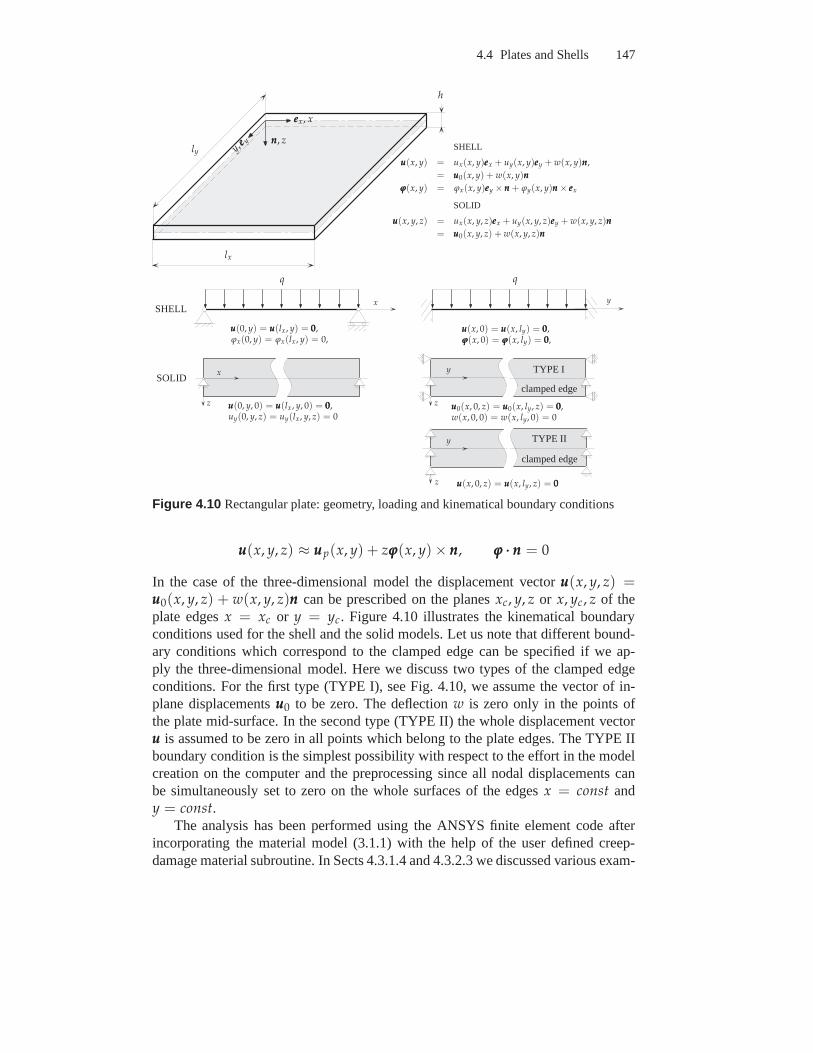
4.4 Plates and Shells 147
eeex, x
y,eee y
x
x
y
y
y
z
zz
nnn, z
lx
ly
h
SHELL
SOLID
uuu(0, y) = uuu(lx, y) = 000,ϕx(0, y) = ϕx(lx, y) = 0,
uuu(x, 0) = uuu(x, ly) = 000,ϕϕϕ(x, 0) = ϕϕϕ(x, ly) = 000,
uuu(0, y, 0) = uuu(lx, y, 0) = 000,uy(0, y, z) = uy(lx, y, z) = 0
uuu0(x, 0, z) = uuu0(x, ly, z) = 000,w(x, 0, 0) = w(x, ly, 0) = 0
uuu(x, 0, z) = uuu(x, ly, z) = 000
TYPE I
clamped edge
clamped edge
TYPE II
SHELL
uuu(x, y) = ux(x, y)eeex + uy(x, y)eeey + w(x, y)nnn,
= uuu0(x, y) + w(x, y)nnn
ϕϕϕ(x, y) = ϕx(x, y)eeey × nnn + ϕy(x, y)nnn × eeex
SOLID
uuu(x, y, z) = ux(x, y, z)eeex + uy(x, y, z)eeey + w(x, y, z)nnn
= uuu0(x, y, z) + w(x, y, z)nnn
Figure 4.10 Rectangular plate: geometry, loading and kinematical boundary conditions
uuu(x, y, z) ≈ uuup(x, y) + zϕϕϕ(x, y) × nnn, ϕϕϕ ··· nnn = 0
In the case of the three-dimensional model the displacementvectoruuu(x, y, z) =uuu0(x, y, z) + w(x, y, z)nnn can be prescribed on the planesxc, y, z or x, yc, z of theplate edgesx = xc or y = yc. Figure 4.10 illustrates the kinematical boundaryconditions used for the shell and the solid models. Let us note that different bound-ary conditions which correspond to the clamped edge can be specified if we ap-ply the three-dimensional model. Here we discuss two types of the clamped edgeconditions. For the first type (TYPE I), see Fig. 4.10, we assume the vector of in-plane displacementsuuu0 to be zero. The deflectionw is zero only in the points ofthe plate mid-surface. In the second type (TYPE II) the wholedisplacement vectoruuu is assumed to be zero in all points which belong to the plate edges. The TYPE IIboundary condition is the simplest possibility with respect to the effort in the modelcreation on the computer and the preprocessing since all nodal displacements canbe simultaneously set to zero on the whole surfaces of the edges x = const andy = const.
The analysis has been performed using the ANSYS finite element code afterincorporating the material model (3.1.1) with the help of the user defined creep-damage material subroutine. In Sects 4.3.1.4 and 4.3.2.3 wediscussed various exam-
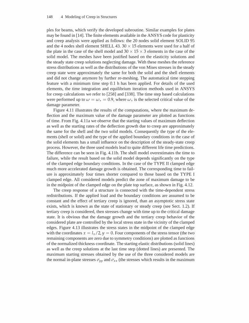
148 4 Modeling of Creep in Structures
ples for beams, which verify the developed subroutine. Similar examples for platesmay be found in [14]. The finite elements available in the ANSYS code for plasticityand creep analysis were applied as follows: the 20 nodes solid element SOLID 95and the 4 nodes shell element SHELL 43.30 × 15 elements were used for a half ofthe plate in the case of the shell model and30 × 15 × 3 elements in the case of thesolid model. The meshes have been justified based on the elasticity solutions andthe steady state creep solutions neglecting damage. With these meshes the referencestress distributions as well as the distributions of the vonMises stresses in the steadycreep state were approximately the same for both the solid and the shell elementsand did not change anymore by further re-meshing. The automatical time steppingfeature with a minimum time step0.1 h has been applied. For details of the usedelements, the time integration and equilibrium iteration methods used in ANSYSfor creep calculations we refer to [258] and [338]. The time step based calculationswere performed up toω = ω∗ = 0.9, whereω∗ is the selected critical value of thedamage parameter.
Figure 4.11 illustrates the results of the computations, where the maximum de-flection and the maximum value of the damage parameter are plotted as functionsof time. From Fig. 4.11a we observe that the starting values of maximum deflectionas well as the starting rates of the deflection growth due to creep are approximatelythe same for the shell and the two solid models. Consequentlythe type of the ele-ments (shell or solid) and the type of the applied boundary conditions in the case ofthe solid elements has a small influence on the description ofthe steady-state creepprocess. However, the three used models lead to quite different life time predictions.The difference can be seen in Fig. 4.11b. The shell model overestimates the time tofailure, while the result based on the solid model depends significantly on the typeof the clamped edge boundary conditions. In the case of the TYPE II clamped edgemuch more accelerated damage growth is obtained. The corresponding time to fail-ure is approximately four times shorter compared to those based on the TYPE Iclamped edge. All considered models predict the zone of maximum damage to bein the midpoint of the clamped edge on the plate top surface, as shown in Fig. 4.12.
The creep response of a structure is connected with the time-dependent stressredistributions. If the applied load and the boundary conditions are assumed to beconstant and the effect of tertiary creep is ignored, than anasymptotic stress stateexists, which is known as the state of stationary or steady creep (see Sect. 1.2). Iftertiary creep is considered, then stresses change with time up to the critical damagestate. It is obvious that the damage growth and the tertiary creep behavior of theconsidered plate are controlled by the local stress state inthe vicinity of the clampededges. Figure 4.13 illustrates the stress states in the midpoint of the clamped edgewith the coordinatesx = lx/2, y = 0. Four components of the stress tensor (the tworemaining components are zero due to symmetry conditions) are plotted as functionsof the normalized thickness coordinate. The starting elastic distributions (solid lines)as well as the creep solutions at the last time step (dotted lines) are presented. Themaximum starting stresses obtained by the use of the three considered models arethe normal in-plane stressesσyy andσxx (the stresses which results in the maximum
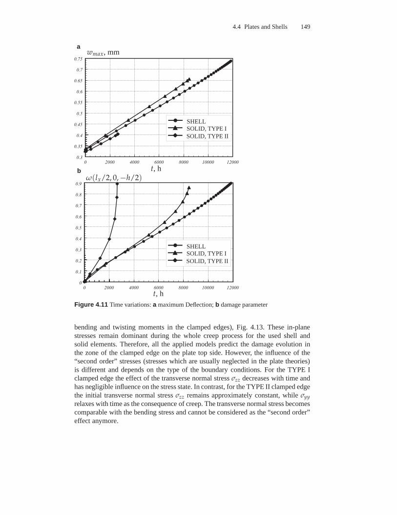
4.4 Plates and Shells 149
0 2 0 0 0 4 0 0 0 6 0 0 0 8 0 0 0 1 0 0 0 0 1 2 0 0 00 . 3
0 . 3 5
0 . 4
0 . 4 5
0 . 5
0 . 5 5
0 . 6
0 . 6 5
0 . 7
0 . 7 5
0 2 0 0 0 4 0 0 0 6 0 0 0 8 0 0 0 1 0 0 0 0 1 2 0 0 00
0 . 1
0 . 2
0 . 3
0 . 4
0 . 5
0 . 6
0 . 7
0 . 8
0 . 9
t, h
t, h
wmax, mm
SHELL
SHELL
SOLID, TYPE I
SOLID, TYPE I
SOLID, TYPE II
SOLID, TYPE II
ω(lx/2, 0,−h/2)
a
b
Figure 4.11 Time variations:a maximum Deflection;b damage parameter
bending and twisting moments in the clamped edges), Fig. 4.13. These in-planestresses remain dominant during the whole creep process forthe used shell andsolid elements. Therefore, all the applied models predict the damage evolution inthe zone of the clamped edge on the plate top side. However, the influence of the“second order” stresses (stresses which are usually neglected in the plate theories)is different and depends on the type of the boundary conditions. For the TYPE Iclamped edge the effect of the transverse normal stressσzz decreases with time andhas negligible influence on the stress state. In contrast, for the TYPE II clamped edgethe initial transverse normal stressσzz remains approximately constant, whileσyy
relaxes with time as the consequence of creep. The transverse normal stress becomescomparable with the bending stress and cannot be consideredas the “second order”effect anymore.
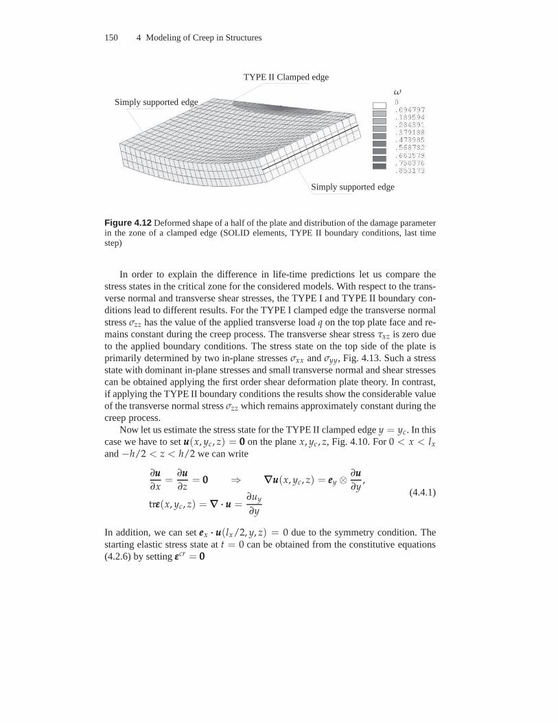
150 4 Modeling of Creep in Structures
ω
TYPE II Clamped edge
Simply supported edge
Simply supported edge
Figure 4.12 Deformed shape of a half of the plate and distribution of the damage parameterin the zone of a clamped edge (SOLID elements, TYPE II boundary conditions, last timestep)
In order to explain the difference in life-time predictionslet us compare thestress states in the critical zone for the considered models. With respect to the trans-verse normal and transverse shear stresses, the TYPE I and TYPE II boundary con-ditions lead to different results. For the TYPE I clamped edge the transverse normalstressσzz has the value of the applied transverse loadq on the top plate face and re-mains constant during the creep process. The transverse shear stressτxz is zero dueto the applied boundary conditions. The stress state on the top side of the plate isprimarily determined by two in-plane stressesσxx andσyy, Fig. 4.13. Such a stressstate with dominant in-plane stresses and small transversenormal and shear stressescan be obtained applying the first order shear deformation plate theory. In contrast,if applying the TYPE II boundary conditions the results showthe considerable valueof the transverse normal stressσzz which remains approximately constant during thecreep process.
Now let us estimate the stress state for the TYPE II clamped edgey = yc. In thiscase we have to setuuu(x, yc, z) = 000 on the planex, yc , z, Fig. 4.10. For0 < x < lx
and−h/2 < z < h/2 we can write
∂uuu
∂x=
∂uuu
∂z= 000 ⇒ ∇∇∇uuu(x, yc, z) = eeey ⊗
∂uuu
∂y,
trεεε(x, yc, z) = ∇∇∇ ··· uuu =∂uy
∂y
(4.4.1)
In addition, we can seteeex ··· uuu(lx/2, y, z) = 0 due to the symmetry condition. Thestarting elastic stress state att = 0 can be obtained from the constitutive equations(4.2.6) by settingεεεcr = 000
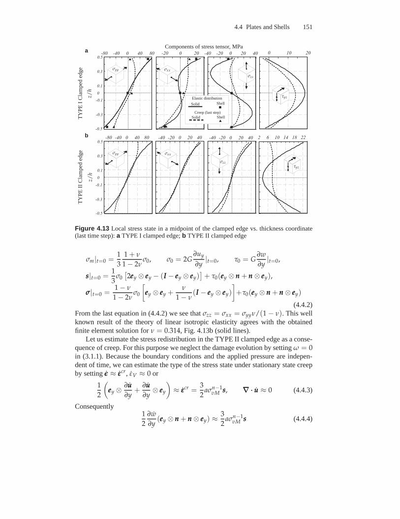
4.4 Plates and Shells 151
0 . 5
0 . 3
0 . 10- 0 . 1
- 0 . 3
- 0 . 5
- 8 0 - 4 0 0 4 0 8 0 - 2 0 0 2 0 - 4 0 - 2 0 0 2 0 4 0 0 1 0 2 0
- 8 0 - 4 0 0 4 0 8 0 - 4 0 - 2 0 0 2 0 4 0 - 4 0 - 2 0 0 2 0 4 0 2 6 1 0 1 4 1 8 2 20 . 5
0 . 3
0 . 10- 0 . 1
- 0 . 3
- 0 . 5
z/h
z/h
TY
PE
ICla
mpe
ded
geT
YP
EII
Cla
mpe
ded
ge
Components of stress tensor, MPa
σyy
σyy
σxx
σxx
σzz
σzz
τyz
τyzElastic distribution
Creep (last step)Solid
Solid
Shell
Shell
a
b
Figure 4.13 Local stress state in a midpoint of the clamped edge vs. thickness coordinate(last time step):a TYPE I clamped edge;b TYPE II clamped edge
σm|t=0 =1
3
1 + ν
1 − 2νσ0, σ0 = 2G
∂uy
∂y|t=0, τ0 = G
∂w
∂y|t=0,
sss|t=0 =1
3σ0
[
2eeey ⊗ eeey − (III − eeey ⊗ eeey)]
+ τ0(eeey ⊗ nnn + nnn ⊗ eeey),
σσσ|t=0 =1 − ν
1 − 2νσ0
[
eeey ⊗ eeey +ν
1 − ν(III − eeey ⊗ eeey)
]
+τ0(eeey ⊗ nnn + nnn ⊗ eeey)
(4.4.2)From the last equation in (4.4.2) we see thatσzz = σxx = σyyν/(1 − ν). This wellknown result of the theory of linear isotropic elasticity agrees with the obtainedfinite element solution forν = 0.314, Fig. 4.13b (solid lines).
Let us estimate the stress redistribution in the TYPE II clamped edge as a conse-quence of creep. For this purpose we neglect the damage evolution by settingω = 0in (3.1.1). Because the boundary conditions and the appliedpressure are indepen-dent of time, we can estimate the type of the stress state under stationary state creepby settingǫǫǫ ≈ εεεcr, εV ≈ 0 or
1
2
(
eeey ⊗∂uuu
∂y+
∂uuu
∂y⊗ eeey
)
≈ εεεcr =3
2aσn−1
vM sss, ∇∇∇ ··· uuu ≈ 0 (4.4.3)
Consequently1
2
∂w
∂y(eeey ⊗ nnn + nnn ⊗ eeey) ≈
3
2aσn−1
vM sss (4.4.4)
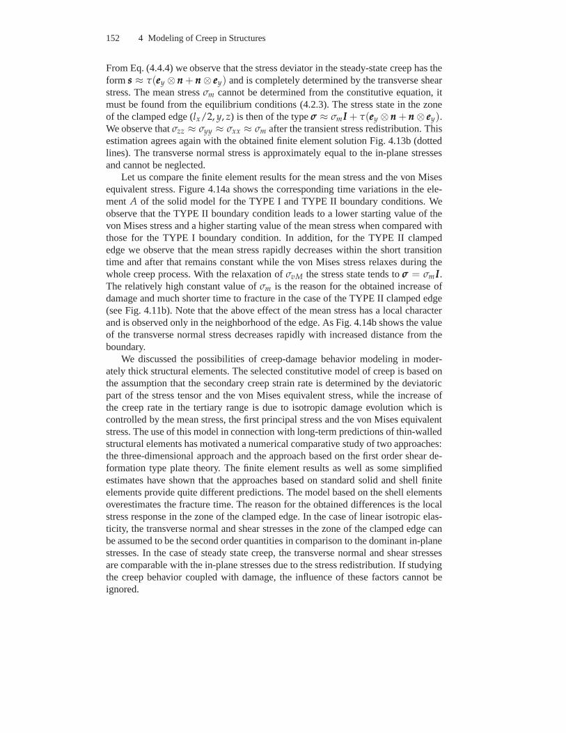
152 4 Modeling of Creep in Structures
From Eq. (4.4.4) we observe that the stress deviator in the steady-state creep has theform sss ≈ τ(eeey ⊗ nnn + nnn ⊗ eeey) and is completely determined by the transverse shearstress. The mean stressσm cannot be determined from the constitutive equation, itmust be found from the equilibrium conditions (4.2.3). The stress state in the zoneof the clamped edge (lx/2, y, z) is then of the typeσσσ ≈ σmIII + τ(eeey ⊗ nnn + nnn ⊗ eeey).We observe thatσzz ≈ σyy ≈ σxx ≈ σm after the transient stress redistribution. Thisestimation agrees again with the obtained finite element solution Fig. 4.13b (dottedlines). The transverse normal stress is approximately equal to the in-plane stressesand cannot be neglected.
Let us compare the finite element results for the mean stress and the von Misesequivalent stress. Figure 4.14a shows the corresponding time variations in the ele-ment A of the solid model for the TYPE I and TYPE II boundary conditions. Weobserve that the TYPE II boundary condition leads to a lower starting value of thevon Mises stress and a higher starting value of the mean stress when compared withthose for the TYPE I boundary condition. In addition, for theTYPE II clampededge we observe that the mean stress rapidly decreases within the short transitiontime and after that remains constant while the von Mises stress relaxes during thewhole creep process. With the relaxation ofσvM the stress state tends toσσσ = σmIII.The relatively high constant value ofσm is the reason for the obtained increase ofdamage and much shorter time to fracture in the case of the TYPE II clamped edge(see Fig. 4.11b). Note that the above effect of the mean stress has a local characterand is observed only in the neighborhood of the edge. As Fig. 4.14b shows the valueof the transverse normal stress decreases rapidly with increased distance from theboundary.
We discussed the possibilities of creep-damage behavior modeling in moder-ately thick structural elements. The selected constitutive model of creep is based onthe assumption that the secondary creep strain rate is determined by the deviatoricpart of the stress tensor and the von Mises equivalent stress, while the increase ofthe creep rate in the tertiary range is due to isotropic damage evolution which iscontrolled by the mean stress, the first principal stress andthe von Mises equivalentstress. The use of this model in connection with long-term predictions of thin-walledstructural elements has motivated a numerical comparativestudy of two approaches:the three-dimensional approach and the approach based on the first order shear de-formation type plate theory. The finite element results as well as some simplifiedestimates have shown that the approaches based on standard solid and shell finiteelements provide quite different predictions. The model based on the shell elementsoverestimates the fracture time. The reason for the obtained differences is the localstress response in the zone of the clamped edge. In the case oflinear isotropic elas-ticity, the transverse normal and shear stresses in the zoneof the clamped edge canbe assumed to be the second order quantities in comparison tothe dominant in-planestresses. In the case of steady state creep, the transverse normal and shear stressesare comparable with the in-plane stresses due to the stress redistribution. If studyingthe creep behavior coupled with damage, the influence of these factors cannot beignored.
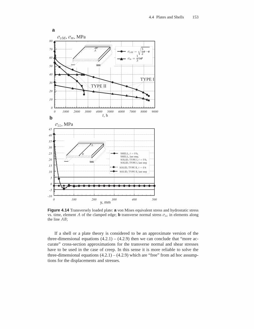
4.4 Plates and Shells 153
0 1 0 0 0 2 0 0 0 3 0 0 0 4 0 0 0 5 0 0 0 6 0 0 0 7 0 0 0 8 0 0 0 9 0 0 00
1 0
2 0
3 0
4 0
5 0
6 0
7 0
8 0
0 1 0 0 2 0 0 3 0 0 4 0 0 5 0 0- 1 0
- 5
0
5
1 0
1 5
2 0
2 5
3 0
3 5
4 0
4 5
y, mm
σzz, MPa
t, h
σvM, σm, MPa
σvM =
√
3
2sss ··· ···sss
σm =1
3trσσσ
SHELL, t = 0 h,SHELL, last step,SOLID, TYPE I,t = 0 h,SOLID, TYPE I, last step
SOLID, TYPE II, t = 0 h
SOLID, TYPE II, last step
A
A
B
TYPE II
TYPE I
a
b
Figure 4.14 Transversely loaded plate:a von Mises equivalent stress and hydrostatic stressvs. time, elementA of the clamped edge;b transverse normal stressσzz in elements alongthe lineAB;
If a shell or a plate theory is considered to be an approximateversion of thethree-dimensional equations (4.2.1) – (4.2.9) then we can conclude that “more ac-curate” cross-section approximations for the transverse normal and shear stresseshave to be used in the case of creep. In this sense it is more reliable to solve thethree-dimensional equations (4.2.1) – (4.2.9) which are “free” from ad hoc assump-tions for the displacements and stresses.
154 4 Modeling of Creep in Structures
4.4.2.2 Long Term Strength Analysis of a Steam Transfer Line . From thepractice of power and petrochemical plants it is well known that pipe bends are themost critical structural components with respect to possible creep failures, e.g. [180,196]. An example for a steam transfer line between a header and a desuperheater ofa boiler is presented in [180]. The pipeline from steel 1Cr0.5Mo (13CrMo4-5) hadoperated under the temperature in the range500 − 550 C and the internal pressure11.8 MPa. After a service life of 77000 h rupture occurred along the outer radius ofa pipe bend. A metallographic analysis of a section cut from the bend close to themain crack has shown typical creep damage due to microvoids and microcracks ongrain boundaries. Several incidents of pipe bend failures in different power plantsare reported in [128]. Inspection techniques were developed to examine the state ofcreep damage during the service. However, as noted in [180],any inspection mustbe conducted at exactly the critical position, or the presence of damage may not bedetected.
Many investigations have addressed the analysis of mechanical behavior of pres-surized curved tubes. Problems of elastic and elasto-platic deformation and stabilityare reviewed in [65, 188]. Creep and creep–damage processesin curved tubes werediscussed in [16, 77, 147, 322]. These studies were concerned with the analysis of asingle pipe bend subjected to special loading conditions, i.e. in-plane bending mo-ments and internal pressure. In the following example we analyze the behavior ofpipe bends in a real spatial pipeline. Figure 4.15 shows the reference geometry ofthe structure which includes three straight pipe segments (I, III and V) and two pipebends (II and IV). The lengths of the pipe segments, the mean diameter of the crosssection and the wall thickness correspond to the data given in [180]. In addition, wetake into account the non-uniformity of the wall thickness in the pipe bends as a re-sult of processing by induction bending. The circumferential thickness distributionis selected according to standard tolerances presented in [41, 115, 196]. The flangesof the pipeline are clamped. The internal pressure and the temperature are assumedto be constant during the creep process. The corresponding values are presented inFig. 4.16. The constitutive model and the material constants for steel 13CrMo4-5 at550 C are taken from [289] (see Sect. 3.1.2).
Figure 4.16 illustrates the deformed shape and the distribution of the magni-tude of the displacement vector in the reference state. Figure 4.17 shows the corre-sponding distribution of the von Mises equivalent stress. From the results we mayconclude that both the pipe bends are subjected to complex spatial loading and de-formation conditions as a result of internal pressure and uniform heating.
Time dependent changes in the deformation and stress statesare illustrated inFigs 4.18 – 4.20. In addition the values of the von Mises equivalent stress in threepoints of the pipe bend IV are plotted as functions of time. According to the resultsthe creep process of the pipeline may be divided into three stages. During the firststage (approximately 50% of the total live) significant stress redistributions occurleading to quite different stress state in the pipeline (cp.Fig. 4.17 and Fig. 4.19).The second stage (approximately 45% of the total live) is characterized by slowchanges in the stress state. In the final stage (approximately 5% of the total live) we
4.4 Plates and Shells 155
observe additional stress redistributions, Fig. 4.20. Thedistribution of the damageparameter at the final time step is shown in Fig. 4.21. According to the results thecritical position of possible creep failure is the pointA of the pipe bend IV. Thisresult agrees well with the data presented in [180], where the creep failure has beendetected at the same position.
Similar processes have been already discussed in Sects 4.3.1.4, 4.3.2.3 and4.4.2.1. One feature of the example considered here is that the final creep stageis not only the result of the local material deterioration but is additionally governedby the flattening (ovalisation) of the pipe bend cross section.
Let us note that some parameters of the reference pipe bend geometries werenot given in [180] and have been assumed in the presented calculation. Further-more, many additional details including the initial out of roundness of the crosssection, inhomogeneous material properties as a result of processing, shutdownsand startups during the service, are not included in the presented model. Thereforethe obtained numerical result for the failure time (49000 h)“slightly” differs fromthe value 77000 h given in [180]. Nevertheless, the results demonstrate the abilityof the modeling to represent basic features of the creep process in a structure and topredict critical zones of possible creep failure.
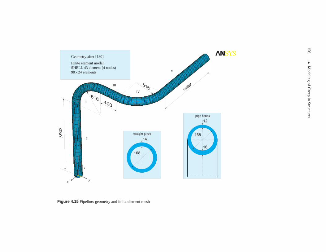
1564
Modeling
ofCreep
inS
tructures
1 6 8
1 41 6 8
1 2
1 6
straight pipes
pipe bends
xy
z
Geometry after [180]
Finite element model:SHELL 43 element (4 nodes)90×24 elements
I
II
III
IV
V
Figure 4.15 Pipeline: geometry and finite element mesh
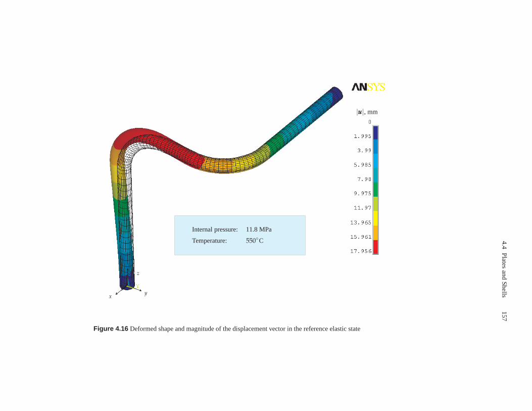
4.4P
latesand
Shells
157
|uuu|, mm
Internal pressure: 11.8 MPa
Temperature: 550C
xy
z
Figure 4.16 Deformed shape and magnitude of the displacement vector in the reference elastic state
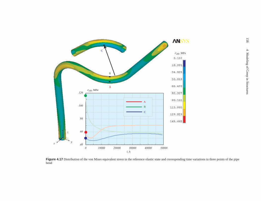
1584
Modeling
ofCreep
inS
tructures
0 1 0 0 0 0 2 0 0 0 0 3 0 0 0 0 4 0 0 0 0 5 0 0 0 04 0
6 0
8 0
1 0 0
1 2 0
t, h
σvM, MPa
σvM, MPa
A
A
B
B
C
C
xy
z
Figure 4.17 Distribution of the von Mises equivalent stress in the reference elastic state and corresponding time variations in three points of the pipebend
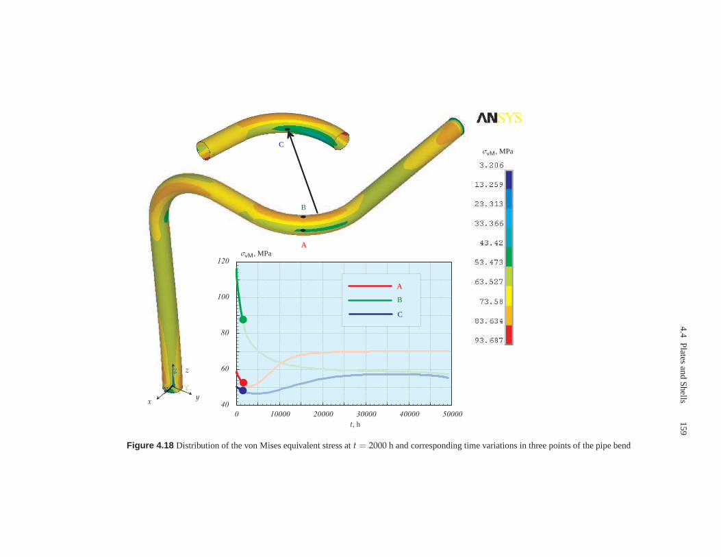
4.4P
latesand
Shells
159
0 1 0 0 0 0 2 0 0 0 0 3 0 0 0 0 4 0 0 0 0 5 0 0 0 04 0
6 0
8 0
1 0 0
1 2 0
t, h
σvM, MPa
σvM, MPa
A
A
B
B
C
C
xy
z
Figure 4.18 Distribution of the von Mises equivalent stress att = 2000 h and corresponding time variations in three points of the pipe bend
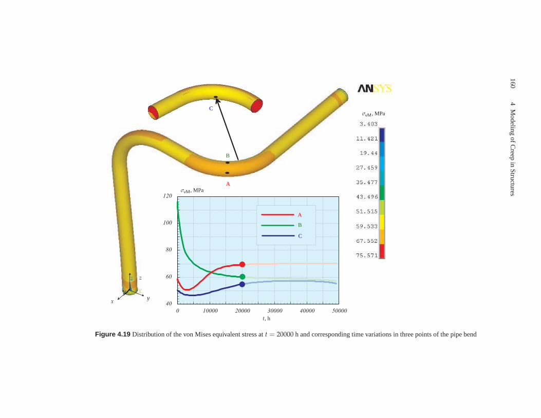
1604
Modeling
ofCreep
inS
tructures
0 1 0 0 0 0 2 0 0 0 0 3 0 0 0 0 4 0 0 0 0 5 0 0 0 04 0
6 0
8 0
1 0 0
1 2 0
t, h
σvM, MPa
σvM, MPa
A
A
B
B
C
C
xy
z
Figure 4.19 Distribution of the von Mises equivalent stress att = 20000 h and corresponding time variations in three points of the pipe bend
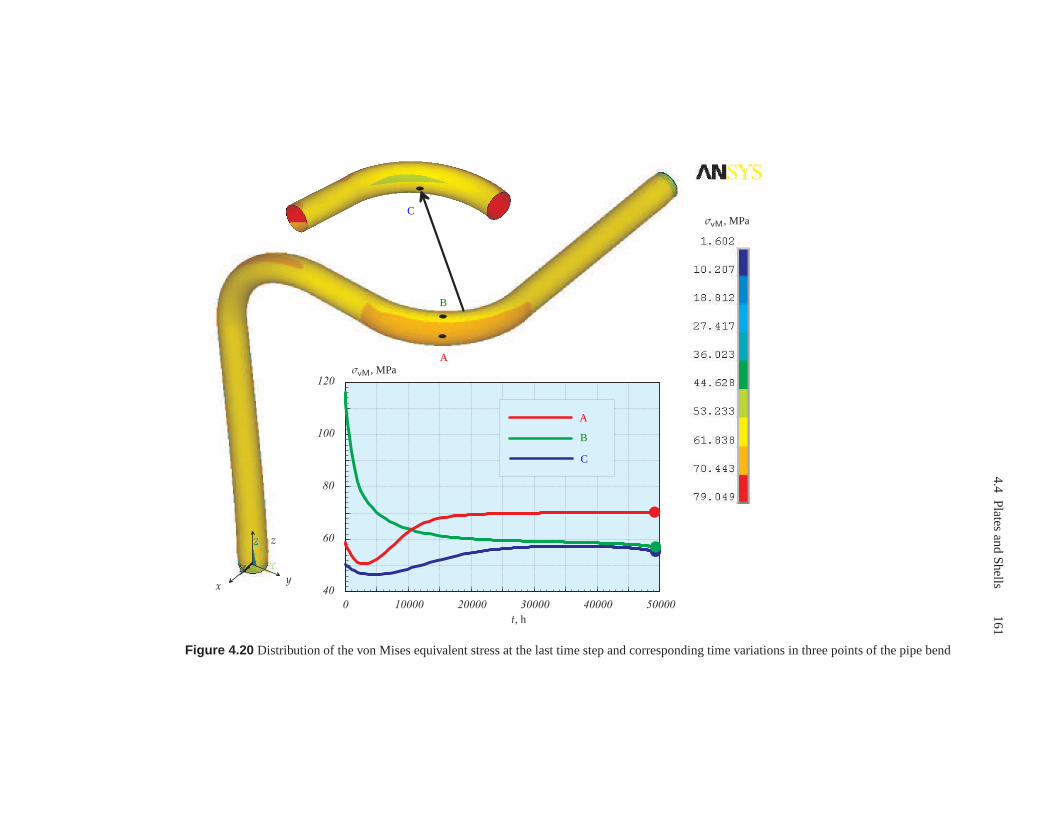
4.4P
latesand
Shells
161
0 1 0 0 0 0 2 0 0 0 0 3 0 0 0 0 4 0 0 0 0 5 0 0 0 04 0
6 0
8 0
1 0 0
1 2 0
t, h
σvM, MPa
σvM, MPa
A
A
B
B
C
C
xy
z
Figure 4.20 Distribution of the von Mises equivalent stress at the last time step and corresponding time variations in three points of the pipe bend
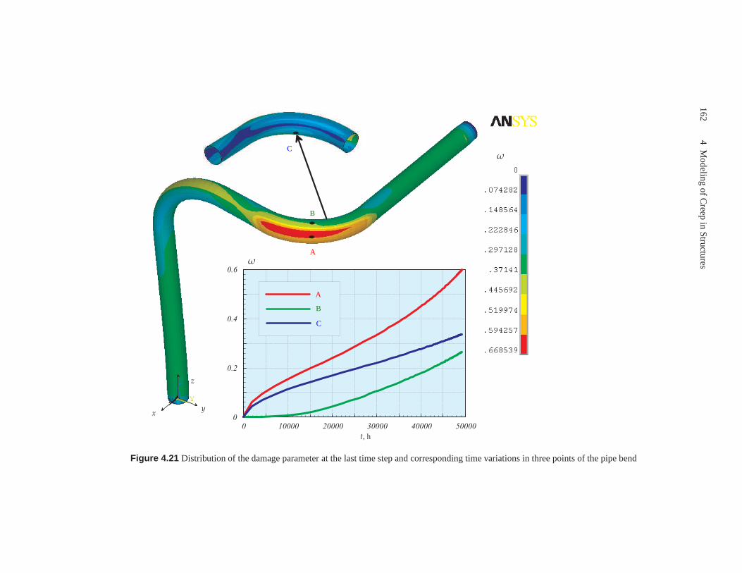
1624
Modeling
ofCreep
inS
tructures
0 1 0 0 0 0 2 0 0 0 0 3 0 0 0 0 4 0 0 0 0 5 0 0 0 00
0 . 2
0 . 4
0 . 6
t, h
ω
ω
A
A
B
B
C
C
xy
z
Figure 4.21 Distribution of the damage parameter at the last time step and corresponding time variations in three points of the pipe bend

5 Conclusions
In this work we discussed models for the analysis of creep andlong-term strengthbehavior of engineering structures under high-temperature conditions. Approachesto formulate
1. Constitutive equations for creep in structural materials,2. Structural mechanics models of beams, plates, shells andthree-dimensional
solids and3. Numerical procedures for the solution of non-linear initial-boundary value
problems
are systematically reviewed and evaluated with respect to their reliability and effi-ciency. Furthermore, we contributed to recent studies in
1. Formulation of multi-axial constitutive equations for creep and damageprocesses which account for stress state effects and anisotropy,
2. Development of a rational framework to find invariants of the stress tensor ap-propriate for constitutive modeling of anisotropic creep,
3. Assessment of several models for beams, plates and shellsin creep and damagerelated structural analysis,
4. Development and verification of creep-damage material subroutines for the usein general purpose finite element codes,
5. Formulation and solution of several problems to illustrate the applicability ofdeveloped techniques
The outcome of our investigations is a numerical method to analyze structural be-havior in the creep-damage range. Several examples illustrate that the developedmethod is capable to reproduce basic features of creep in engineering structuresincluding time-dependent changes in shape, stress redistributions and formation ofcritical zones of possible creep failure.
Let us summarize the main conclusions of our study and some recommendations
1. The accurate description of creep and damage processes instructural materialsrequires accurate data obtained from creep tests. Regardless of which phenom-enological approach to formulate the constitutive equation (e.g. “pure phenom-enological”, “mechanism-based” or “micromechanically-consistent”) is used,the choice of the response function, the introduction of theequivalent stressand the identification of material constants require material data over a wide
164 5 Conclusions
range of stresses, stress states and temperatures. As illustrated in Sect. 3.1.4 theavailable creep curves for an aluminium alloy can be described by different ma-terial models with the same accuracy. In this sense no preference can be madebetween different approaches to constitutive equations. However, in structuralanalysis applications, different constitutive models maylead to quite differentlife time estimations (see Sect. 3.1.4). Therefore the question of what approachshould be selected to formulate constitutive equations canonly be discussed inconnection with the structural mechanics analysis.Further investigations are required to assess recently proposed constitutivemodels as they predict creep and long term strength for different types of struc-tures.
2. Hardening and damage processes have in general anisotropic nature since theyare associated with topological changes of the microstructure. Isotropic consti-tutive models of creep have been found to be inappropriate indescribing exper-imental data from tests under non-proportional loading conditions. Thereforein many works it is suggested to operate with hardening and damage tensorsinstead of scalars. Let us note that the principal role of tensor-valued internalstate variables is to reflect the local changes of material symmetries during thecreep process. However, the available experimental data hardly allow to verifyboth the type of the assumed symmetry (e.g. isotropy, transverse isotropy, or-thotropic symmetry, etc.) and the orientation of symmetry planes or axes. Theproposed kinematic hardening rules and damage evolution equations are suffi-cient to characterize creep behavior under simple monotonic or cyclic loading.However, they are poorly suited for the description of transient creep effectsunder non-proportional loading conditions.
3. Refined models for beams, plates and shells including effects of the transverseshear deformation and geometrical non-linearities shouldbe preferred in longterm strength analysis of thinwalled structures. For beamsthe effects of trans-verse shear deformation has been illustrated in Sect. 4.3.2.3. Several examplesfor plates and shells presented in the literature (see Sect.4.4.1) show that even inthe case of “moderate” bending, the classical geometrically-linear theory leadsto a significant underestimation of the life-time and overestimation of the defor-mation. Further benchmark problems which are able to reproduce the behaviorof boundary layers in the creep range are required. They could be useful in theassessment of different available shell type finite elements.
4. Numerical solutions of creep-damage problems by the finite element methodare highly sensitive to the mesh density. A mesh which provides satisfactoryaccurate results in the linear-elastic range is not sufficient to solve creep prob-lems (see Sect. 4.3.1.4). Furthermore, the mesh density required for an accuratesolution depends not only on the geometry and loading of the structure but alsoon the type of the applied creep constitutive equation. Whenstudying creep-damage in structures with complex geometry it is difficult totest the mesh sen-sitivity and prove the solution convergence due to large computational time.From our experience we may recommend to adjust the mesh to theconvergent
5. Conclusions 165
solution in the steady-state creep range. With such meshes the accuracy of long-term predictions was not less than the accuracy of the material data involved inthe computations.
The currently available approaches of creep mechanics are helpful in understandingmechanisms of structural behavior under creep and damage conditions and can berecommended for design and remnant life assessments of structures. Results of ourstudy could lead to further investigations with the following topics
1. Consideration of manufacturing conditions as they influence the subsequentcreep behavior of structures. In the example presented in Sect. 4.4.2.2 the wallthinning due to processing of the pipe bend was taken into account. It would beof interest to examine the influence of other factors determined by processing,e.g. initial out of roundness and inhomogeneous material properties.A model developed in Sect. 3.2 could be the basis of further studies of creepin welded structures by taking into account the initial anisotropy in multi-passweld metals.
2. Several databases exist, where experiences from engineering practice in powerand petrochemical plants are collected for a wide range of structures. With thegained experience in modeling and numerical analysis of creep it is possibleand useful to analyze recently documented cases of creep failures. Such studiescould provide new suggestions in the creep constitutive modeling and stimulatefurther experimental investigations.

166 5 Conclusions
A Some Basic Rules of Tensor Calculus
The tensor calculus is a powerful tool for the description ofthe fundamentals in con-tinuum mechanics and the derivation of the governing equations for applied prob-lems. In general, there are two possibilities for the representation of the tensors andthe tensorial equations:
– the direct (symbolic) notation and– the index (component) notation
The direct notation operates with scalars, vectors and tensors as physical objectsdefined in the three dimensional space. A vector (first rank tensor)aaa is consideredas a directed line segment rather than a triple of numbers (coordinates). A secondrank tensorAAA is any finite sum of ordered vector pairsAAA = a ⊗ ba ⊗ ba ⊗ b + . . . + c ⊗ dc ⊗ dc ⊗ d. Thescalars, vectors and tensors are handled as invariant (independent from the choice ofthe coordinate system) objects. This is the reason for the use of the direct notationin the modern literature of mechanics and rheology, e.g. [29, 32, 49, 123, 131, 199,246, 313, 334] among others.
The index notation deals with components or coordinates of vectors and tensors.For a selected basis, e.g.gggi, i = 1, 2, 3 one can write
aaa = aigggi, AAA =(
aibj + . . . + cidj)
gggi ⊗ gggj
Here the Einstein’s summation convention is used: in one expression the twice re-peated indices are summed up from 1 to 3, e.g.
akgggk ≡3
∑k=1
akgggk, Aikbk ≡3
∑k=1
Aikbk
In the above examplesk is a so-called dummy index. Within the index notation thebasic operations with tensors are defined with respect to their coordinates, e. g. thesum of two vectors is computed as a sum of their coordinatesci = ai + bi. Theintroduced basis remains in the background. It must be remembered that a changeof the coordinate system leads to the change of the components of tensors.
In this work we prefer the direct tensor notation over the index one. When solv-ing applied problems the tensor equations can be “translated” into the languageof matrices for a specified coordinate system. The purpose ofthis Appendix is to
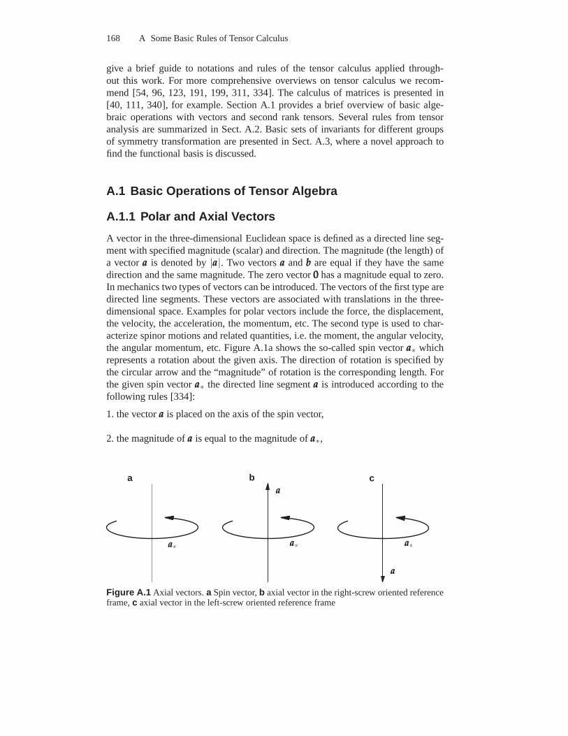
168 A Some Basic Rules of Tensor Calculus
give a brief guide to notations and rules of the tensor calculus applied through-out this work. For more comprehensive overviews on tensor calculus we recom-mend [54, 96, 123, 191, 199, 311, 334]. The calculus of matrices is presented in[40, 111, 340], for example. Section A.1 provides a brief overview of basic alge-braic operations with vectors and second rank tensors. Several rules from tensoranalysis are summarized in Sect. A.2. Basic sets of invariants for different groupsof symmetry transformation are presented in Sect. A.3, where a novel approach tofind the functional basis is discussed.
A.1 Basic Operations of Tensor Algebra
A.1.1 Polar and Axial Vectors
A vector in the three-dimensional Euclidean space is definedas a directed line seg-ment with specified magnitude (scalar) and direction. The magnitude (the length) ofa vectoraaa is denoted by|aaa|. Two vectorsaaa andbbb are equal if they have the samedirection and the same magnitude. The zero vector000 has a magnitude equal to zero.In mechanics two types of vectors can be introduced. The vectors of the first type aredirected line segments. These vectors are associated with translations in the three-dimensional space. Examples for polar vectors include the force, the displacement,the velocity, the acceleration, the momentum, etc. The second type is used to char-acterize spinor motions and related quantities, i.e. the moment, the angular velocity,the angular momentum, etc. Figure A.1a shows the so-called spin vectoraaa∗ whichrepresents a rotation about the given axis. The direction ofrotation is specified bythe circular arrow and the “magnitude” of rotation is the corresponding length. Forthe given spin vectoraaa∗ the directed line segmentaaa is introduced according to thefollowing rules [334]:
1. the vectoraaa is placed on the axis of the spin vector,
2. the magnitude ofaaa is equal to the magnitude ofaaa∗,
aaa∗aaa∗aaa∗
aaa
aaa
a b c
Figure A.1 Axial vectors.a Spin vector,b axial vector in the right-screw oriented referenceframe,c axial vector in the left-screw oriented reference frame
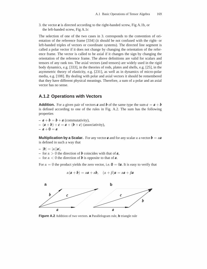
A.1 Basic Operations of Tensor Algebra 169
3. the vectoraaa is directed according to the right-handed screw, Fig A.1b, orthe left-handed screw, Fig A.1c
The selection of one of the two cases in 3. corresponds to the convention of ori-entation of the reference frame [334] (it should be not confused with the right- orleft-handed triples of vectors or coordinate systems). Thedirected line segment iscalled a polar vector if it does not change by changing the orientation of the refer-ence frame. The vector is called to be axial if it changes the sign by changing theorientation of the reference frame. The above definitions are valid for scalars andtensors of any rank too. The axial vectors (and tensors) are widely used in the rigidbody dynamics, e.g. [333], in the theories of rods, plates and shells, e.g. [25], in theasymmetric theory of elasticity, e.g. [231], as well as in dynamics of micro-polarmedia, e.g. [108]. By dealing with polar and axial vectors itshould be rememberedthat they have different physical meanings. Therefore, a sum of a polar and an axialvector has no sense.
A.1.2 Operations with Vectors
Addition. For a given pair of vectorsaaa andbbb of the same type the sumccc = aaa + bbbis defined according to one of the rules in Fig. A.2. The sum hasthe followingproperties
– aaa + bbb = bbb + aaa (commutativity),– (aaa + bbb) + ccc = aaa + (bbb + ccc) (associativity),– aaa + 000 = aaa
Multiplication by a Scalar. For any vectoraaa and for any scalarα a vectorbbb = αaaais defined in such a way that
– |bbb| = |α||aaa|,– for α > 0 the direction ofbbb coincides with that ofaaa,– for α < 0 the direction ofbbb is opposite to that ofaaa.
For α = 0 the product yields the zero vector, i.e.000 = 0aaa. It is easy to verify that
α(aaa + bbb) = αaaa + αbbb, (α + β)aaa = αaaa + βaaa
aaaaaa
bbb
bbb cccccc
a b
Figure A.2 Addition of two vectors.a Parallelogram rule,b triangle rule
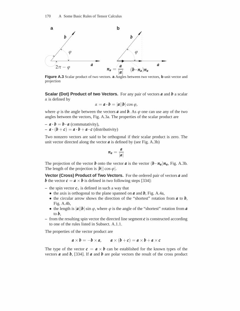
170 A Some Basic Rules of Tensor Calculus
aaaaaa
bbbbbb
ϕϕ
2π − ϕ nnnaaa =aaa
|aaa| (bbb ··· nnnaaa)nnnaaa
a b
Figure A.3 Scalar product of two vectors.a Angles between two vectors,b unit vector andprojection
Scalar (Dot) Product of two Vectors. For any pair of vectorsaaa andbbb a scalarα is defined by
α = aaa ··· bbb = |aaa||bbb| cos ϕ,
whereϕ is the angle between the vectorsaaa andbbb. As ϕ one can use any of the twoangles between the vectors, Fig. A.3a. The properties of thescalar product are
– aaa ··· bbb = bbb ··· aaa (commutativity),– aaa ··· (bbb + ccc) = aaa ··· bbb + aaa ··· ccc (distributivity)
Two nonzero vectors are said to be orthogonal if their scalarproduct is zero. Theunit vector directed along the vectoraaa is defined by (see Fig. A.3b)
nnnaaa =aaa
|aaa|
The projection of the vectorbbb onto the vectoraaa is the vector(bbb ··· nnnaaa)nnnaaa, Fig. A.3b.The length of the projection is|bbb|| cos ϕ|.Vector (Cross) Product of Two Vectors. For the ordered pair of vectorsaaa andbbb the vectorccc = aaa × bbb is defined in two following steps [334]:
– the spin vectorccc∗ is defined in such a way that• the axis is orthogonal to the plane spanned onaaa andbbb, Fig. A.4a,• the circular arrow shows the direction of the “shortest” rotation fromaaa to bbb,
Fig. A.4b,• the length is|aaa||bbb| sin ϕ, whereϕ is the angle of the “shortest” rotation fromaaa
to bbb,– from the resulting spin vector the directed line segmentccc is constructed according
to one of the rules listed in Subsect. A.1.1.
The properties of the vector product are
aaa × bbb = −bbb × aaa, aaa × (bbb + ccc) = aaa × bbb + aaa × ccc
The type of the vectorccc = aaa × bbb can be established for the known types of thevectorsaaa andbbb, [334]. If aaa andbbb are polar vectors the result of the cross product
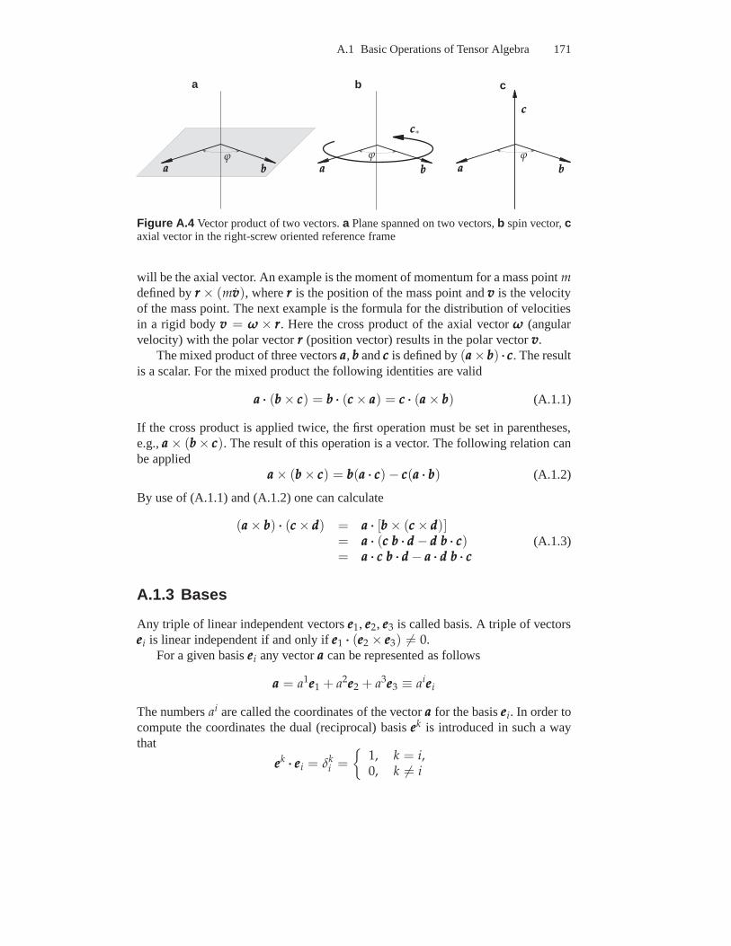
A.1 Basic Operations of Tensor Algebra 171
aaaaaaaaa bbbbbbbbbϕϕϕ
ccc∗
ccc
a b c
Figure A.4 Vector product of two vectors.a Plane spanned on two vectors,b spin vector,caxial vector in the right-screw oriented reference frame
will be the axial vector. An example is the moment of momentumfor a mass pointmdefined byrrr × (mvvv), whererrr is the position of the mass point andvvv is the velocityof the mass point. The next example is the formula for the distribution of velocitiesin a rigid bodyvvv = ωωω × rrr. Here the cross product of the axial vectorωωω (angularvelocity) with the polar vectorrrr (position vector) results in the polar vectorvvv.
The mixed product of three vectorsaaa, bbb andccc is defined by(aaa × bbb) ··· ccc. The resultis a scalar. For the mixed product the following identities are valid
aaa ··· (bbb × ccc) = bbb ··· (ccc × aaa) = ccc ··· (aaa × bbb) (A.1.1)
If the cross product is applied twice, the first operation must be set in parentheses,e.g.,aaa × (bbb × ccc). The result of this operation is a vector. The following relation canbe applied
aaa × (bbb × ccc) = bbb(aaa ··· ccc) − ccc(aaa ··· bbb) (A.1.2)
By use of (A.1.1) and (A.1.2) one can calculate
(aaa × bbb) ··· (ccc × ddd) = aaa ··· [bbb × (ccc × ddd)]= aaa ··· (ccc bbb ··· ddd − ddd bbb ··· ccc)= aaa ··· ccc bbb ··· ddd − aaa ··· ddd bbb ··· ccc
(A.1.3)
A.1.3 Bases
Any triple of linear independent vectorseee1, eee2, eee3 is called basis. A triple of vectorseeei is linear independent if and only ifeee1 ··· (eee2 × eee3) 6= 0.
For a given basiseeei any vectoraaa can be represented as follows
aaa = a1eee1 + a2eee2 + a3eee3 ≡ aieeei
The numbersai are called the coordinates of the vectoraaa for the basiseeei. In order tocompute the coordinates the dual (reciprocal) basiseeek is introduced in such a waythat
eeek ··· eeei = δki =
1, k = i,0, k 6= i
172 A Some Basic Rules of Tensor Calculus
δki is the Kronecker symbol. The coordinatesai can be found by
eeei ··· aaa = aaa ··· eeei = ameeem · eeei = amδim = ai
For the selected basiseeei the dual basis can be found from
eee1 =eee2 × eee3
(eee1 × eee2) ··· eee3, eee2 =
eee3 × eee1
(eee1 × eee2) ··· eee3, eee3 =
eee1 × eee2
(eee1 × eee2) ··· eee3(A.1.4)
By use of the dual basis a vectoraaa can be represented as follows
aaa = a1eee1 + a2eee2 + a3eee3 ≡ aieeei, am = aaa ··· eeem, am 6= am
In the special case of the orthonormal vectorseeei, i.e. |eeei| = 1 andeeei ··· eeek = 0 fori 6= k, from (A.1.4) follows thateeek = eeek and consequentlyak = ak.
A.1.4 Operations with Second Rank Tensors
A second rank tensor is a finite sum of ordered vector pairsAAA = aaa⊗bbb + . . . + ccc⊗ddd[334]. One ordered pair of vectors is called the dyad. The symbol ⊗ is called thedyadic (tensor) product of two vectors. A single dyad or a sumof two dyads arespecial cases of the second rank tensor. Any finite sum of morethan three dyads canbe reduced to a sum of three dyads. For example, let
AAA =n
∑i=1
aaa(i) ⊗ bbb(i)
be a second rank tensor. Introducing a basiseeek the vectorsaaa(i) can be represented
by aaa(i) = ak(i)
eeek, whereak(i)
are coordinates of the vectorsaaa(i). Now we may write
AAA =n
∑i=1
ak(i)eeek ⊗ bbb(i) = eeek ⊗
n
∑i=1
ak(i)bbb(i) = eeek ⊗ dddk, dddk ≡
n
∑i=1
ak(i)bbb(i)
Addition. The sum of two tensors is defined as the sum of the correspondingdyads. The sum has the properties of associativity and commutativity. In addition,for a dyadaaa ⊗ bbb the following operation is introduced
aaa ⊗ (bbb + ccc) = aaa ⊗ bbb + aaa ⊗ ccc, (aaa + bbb)⊗ ccc = aaa ⊗ ccc + bbb ⊗ ccc
Multiplication by a Scalar. This operation is introduced first for one dyad. Forany scalarα and any dyadaaa ⊗ bbb
α(aaa ⊗ bbb) = (αaaa) ⊗ bbb = aaa ⊗ (αbbb),(α + β)aaa ⊗ bbb = αaaa ⊗ bbb + βaaa ⊗ bbb
(A.1.5)
By settingα = 0 in the first equation of (A.1.5) the zero dyad can be defined, i.e.0(aaa ⊗ bbb) = 000 ⊗ bbb = aaa ⊗ 000. The above operations can be generalized for any finitesum of dyads, i.e. for second rank tensors.
A.1 Basic Operations of Tensor Algebra 173
Inner Dot Product. For any two second rank tensorsAAA andBBB the inner dot prod-uct is specified byAAA ··· BBB. The rule and the result of this operation can be explainedin the special case of two dyads, i.e. by settingAAA = aaa ⊗ bbb andBBB = ccc ⊗ ddd
AAA ··· BBB = aaa ⊗ bbb ··· ccc ⊗ ddd = (bbb ··· ccc)aaa ⊗ ddd = αaaa ⊗ ddd, α ≡ bbb ··· ccc
The result of this operation is a second rank tensor. Note that AAA · BBB 6= BBB · AAA. Thiscan be again verified for two dyads. The operation can be generalized for two secondrank tensors as follows
AAA ··· BBB =3
∑i=1
aaa(i) ⊗ bbb(i) ···3
∑k=1
ccc(k) ⊗ ddd(k) =3
∑i=1
3
∑k=1
(bbb(i) ··· ccc(k))aaa(i) ⊗ ddd(k)
Transpose of a Second Rank Tensor. The transpose of a second rank tensorAAA is constructed by the following rule
AAAT =
(
3
∑i=1
aaa(i) ⊗ bbb(i)
)T
=3
∑i=1
bbb(i) ⊗ aaa(i)
Double Inner Dot Product. For any two second rank tensorsAAA andBBB the doubleinner dot product is specified byAAA ······ BBB The result of this operation is a scalar. Thisoperation can be explained for two dyads as follows
AAA ······ BBB = aaa ⊗ bbb ······ ccc ⊗ ddd = (bbb ··· ccc)(aaa ··· ddd)
By analogy to the inner dot product one can generalize this operation for two secondrank tensors. It can be verified thatAAA ······ BBB = BBB ······ AAA for second rank tensorsAAA andBBB. For a second rank tensorAAA and for a dyadaaa ⊗ bbb
AAA ······ aaa ⊗ bbb = bbb ··· AAA ··· aaa (A.1.6)
A scalar product of two second rank tensorsAAA andBBB is defined by
α = AAA ······ BBBT
One can verify thatAAA ······ BBBT = BBBT ······ AAA = BBB ······ AAAT
Dot Products of a Second Rank Tensor and a Vector. The right dot productof a second rank tensorAAA and a vectorccc is defined by
AAA ··· ccc =
(
3
∑i=1
aaa(i) ⊗ bbb(i)
)
··· ccc =3
∑i=1
(bbb(i) ··· ccc)aaa(i)
For a single dyad this operation is
aaa ⊗ bbb ··· ccc = aaa(bbb ··· ccc)
174 A Some Basic Rules of Tensor Calculus
The left dot product is defined by
ccc ··· AAA = ccc ···(
3
∑i=1
aaa(i) ⊗ bbb(i)
)
=3
∑i=1
(ccc ··· aaa(i))bbb(i)
The results of these operations are vectors. One can verify that
AAA ··· ccc 6= ccc ··· AAA, AAA ··· ccc = ccc ··· AAAT
Cross Products of a Second Rank Tensor and a Vector. The right crossproduct of a second rank tensorAAA and a vectorccc is defined by
AAA × ccc =
(
3
∑i=1
aaa(i) ⊗ bbb(i)
)
× ccc =3
∑i=1
aaa(i) ⊗ (bbb(i) × ccc)
The left cross product is defined by
ccc × AAA = ccc ×(
3
∑i=1
aaa(i) ⊗ bbb(i)
)
=3
∑i=1
(ccc × aaa(i))⊗ bbb(i)
The results of these operations are second rank tensors. It can be shown that
AAA × ccc = −[ccc × AAAT ]T
Trace. The trace of a second rank tensor is defined by
tr AAA = tr
(
3
∑i=1
aaa(i) ⊗ bbb(i)
)
=3
∑i=1
aaa(i) ··· bbb(i)
By taking the trace of a second rank tensor the dyadic productis replaced by the dotproduct. It can be shown that
tr AAA = tr AAAT, tr (AAA ··· BBB) = tr (BBB ··· AAA) = tr (AAAT ··· BBBT) = AAA ······ BBB
Symmetric Tensors. A second rank tensor is said to be symmetric if it satisfiesthe following equality
AAA = AAAT
An alternative definition of the symmetric tensor can be given as follows. A secondrank tensor is said to be symmetric if for any vectorccc 6= 000 the following equality isvalid
ccc ··· AAA = AAA · ccc
An important example of a symmetric tensor is the unit or identity tensorIII, whichis defined by such a way that for any vectorccc
ccc ··· III = III ··· ccc = ccc
A.1 Basic Operations of Tensor Algebra 175
The representations of the identity tensor are
III = eeek ⊗ eeek = eeek ⊗ eeek
for any basiseeek andeeek, eeek ··· eeem = δmk . For three orthonormal vectorsmmm, nnn andppp
III = nnn ⊗ nnn + mmm ⊗mmm + ppp ⊗ ppp
A symmetric second rank tensorPPP satisfying the conditionPPP ··· PPP = PPP is calledprojector. Examples of projectors are
mmm ⊗mmm, nnn ⊗ nnn + ppp ⊗ ppp = III −mmm ⊗mmm,
wheremmm, nnn andppp are orthonormal vectors. The result of the dot product of thetensormmm ⊗mmm with any vectoraaa is the projection of the vectoraaa onto the line spanned onthe vectormmm, i.e.mmm ⊗mmm ··· aaa = (aaa ··· mmm)mmm. The result of(nnn ⊗ nnn + ppp ⊗ ppp) ··· aaa is theprojection of the vectoraaa onto the plane spanned on the vectorsnnn andppp.
Skew-symmetric Tensors. A second rank tensor is said to be skew-symmetricif it satisfies the following equality
AAA = −AAAT
or if for any vectorcccccc ··· AAA = −AAA · ccc
Any skew symmetric tensorAAA can be represented by
AAA = aaa × III = III × aaa
The vectoraaa is called the associated vector. Any second rank tensor can be uniquelydecomposed into the symmetric and skew-symmetric parts
AAA =1
2
(
AAA + AAAT)
+1
2
(
AAA − AAAT)
= AAA1 + AAA2,
AAA1 =1
2
(
AAA + AAAT)
, AAA1 = AAAT1 ,
AAA2 =1
2
(
AAA − AAAT)
, AAA2 = −AAAT2
Vector Invariant. The vector invariant or “Gibbsian Cross” of a second rank ten-sorAAA is defined by
AAA× =
(
3
∑i=1
aaa(i) ⊗ bbb(i)
)
×=
3
∑i=1
aaa(i) × bbb(i)
The result of this operation is a vector. The vector invariant of a symmetric tensor isthe zero vector. The following identities can be verified
(aaa × III)× = −2aaa, aaa × III × bbb = bbb ⊗ aaa − (aaa ··· bbb)III
176 A Some Basic Rules of Tensor Calculus
Linear Transformations of Vectors. A vector valued function of a vector ar-gumentfff (aaa) is called to be linear iffff (α1aaa1 + α2aaa2) = α1 fff (aaa1) + α2 fff (aaa2) for anytwo vectorsaaa1 andaaa2 and any two scalarsα1 andα2. It can be shown that any linearvector valued function can be represented byfff (aaa) = AAA ··· aaa, whereAAA is a secondrank tensor. In many textbooks, e.g. [32, 293] a second rank tensorAAA is defined tobe the linear transformation of the vector space into itself.
Determinant and Inverse of a Second Rank Tensor. Let aaa, bbb andccc be ar-bitrary linearly-independent vectors. The determinant ofa second rank tensorAAA isdefined by
det AAA =(AAA ··· aaa) ··· [(AAA ··· bbb)× (AAA ··· ccc)]
aaa ··· (bbb × ccc)
The following identities can be verified
det(AAAT) = det(AAA), det(AAA ··· BBB) = det(AAA) det(BBB)
The inverse of a second rank tensorAAA−1 is introduced as the solution of the follow-ing equation
AAA−1 ··· AAA = AAA ··· AAA−1 = III
AAA is invertible if and only ifdet AAA 6= 0. A tensorAAA with det AAA = 0 is calledsingular. Examples of singular tensors are projectors.
Cayley-Hamilton Theorem. Any second rank tensor satisfies the followingequation
AAA3 − J1(AAA)AAA2 + J2(AAA)AAA − J3(AAA)III = 000, (A.1.7)
whereAAA2 = AAA ··· AAA, AAA3 = AAA ··· AAA ··· AAA and
J1(AAA) = tr AAA, J2(AAA) =1
2[(tr AAA)2 − tr AAA2],
J3(AAA) = det AAA =1
6(tr AAA)3 − 1
2tr AAAtr AAA2 +
1
3tr AAA3
(A.1.8)
The scalar-valued functionsJi(AAA) are called principal invariants of the tensorAAA.
Coordinates of Second Rank Tensors. Let eeei be a basis andeeek the dual basis.Any two vectorsaaa andbbb can be represented as follows
aaa = aieeei = ajeeej, bbb = bleeel = bmeeem
A dyadaaa ⊗ bbb has the following representations
aaa ⊗ bbb = aibjeeei ⊗ eeej = aibjeeei ⊗ eeej = aibjeeei ⊗ eeej = aib
jeeei ⊗ eeej
For the representation of a second rank tensorAAA one of the following four bases canbe used
eeei ⊗ eeej, eeei ⊗ eeej, eeei ⊗ eeej, eeei ⊗ eeej
With these bases one can write
A.1 Basic Operations of Tensor Algebra 177
AAA = Aijeeei ⊗ eeej = Aijeeei ⊗ eeej = Ai∗
∗jeeei ⊗ eeej = A∗ji∗eeei ⊗ eeej
For a selected basis the coordinates of a second rank tensor can be computed asfollows
Aij = eeei ··· AAA · eeej, Aij = eeei ··· AAA · eeej,
Ai∗∗j = eeei ··· AAA · eeej, A
∗ji∗ = eeei ··· AAA · eeej
Principal Values and Directions of Symmetric Second Rank Te nsors.Consider a dot product of a second rank tensorAAA and a unit vectornnn. The resultingvectoraaa = AAA ··· nnn differs in general fromnnn both by the length and the direction.However, one can find those unit vectorsnnn, for which AAA ··· nnn is collinear withnnn, i.e.only the length ofnnn is changed. Such vectors can be found from the equation
AAA ··· nnn = λnnn or (AAA − λIII) ··· nnn = 000 (A.1.9)
The unit vectornnn is called the principal vector and the scalarλ the principal valueof the tensorAAA. Let AAA be a symmetric tensor. In this case the principal values arereal numbers and there exist at least three mutually orthogonal principal vectors.The principal values can be found as roots of the characteristic polynomial
det(AAA − λIII) = −λ3 + J1(AAA)λ2 − J2(AAA)λ + J3(AAA) = 0
The principal values are specified byλI , λI I , λI I I . For known principal values andprincipal directions the second rank tensor can be represented as follows (spectralrepresentation)
AAA = λInnnI ⊗ nnnI + λI InnnI I ⊗ nnnI I + λI I InnnI I I ⊗ nnnI I I
Orthogonal Tensors. A second rank tensorQQQ is said to be orthogonal if it sat-isfies the equationQQQT ··· QQQ = III. If QQQ operates on a vector its length remains un-changed, i.e. letbbb = QQQ ··· aaa, then
|bbb|2 = bbb ··· bbb = aaa ··· QQQT ···QQQ ··· aaa = aaa ··· aaa = |aaa|2
Furthermore, the orthogonal tensor does not change the scalar product of two arbi-trary vectors. For two vectorsaaa andbbb as well asaaa′ = QQQ ··· aaa andbbb′ = QQQ ··· bbb one cancalculate
aaa′ ··· bbb′ = aaa ···QQQT ···QQQ ··· bbb = aaa ··· bbb
From the definition of the orthogonal tensor follows
QQQT = QQQ−1, QQQT ···QQQ = QQQ ···QQQT = III,
det(QQQ ··· QQQT) = (det QQQ)2 = det III = 1 ⇒ det QQQ = ±1
Orthogonal tensors withdet QQQ = 1 are called proper orthogonal or rotation tensors.The rotation tensors are widely used in the rigid body dynamics, e.g. [333], and inthe theories of rods, plates and shells, e.g. [25, 32]. Any orthogonal tensor is either
178 A Some Basic Rules of Tensor Calculus
the rotation tensor or the composition of the rotation (proper orthogonal tensor) andthe tensor−III. Let PPP be a rotation tensor,det PPP = 1, then an orthogonal tensorQQQwith detQQQ = −1 can be composed by
QQQ = (−III) ··· PPP = PPP ··· (−III), det QQQ = det(−−−I) det PPP = −1
For any two orthogonal tensorsQQQ1 andQQQ2 the compositionQQQ3 = QQQ1 ···QQQ2 is the or-thogonal tensor, too. This property is used in the theory of symmetry and symmetrygroups, e.g. [232, 331]. Two important examples for orthogonal tensors are
• rotation tensor about a fixed axis
QQQ(ψmmm) = mmm ⊗mmm + cos ψ(III −mmm ⊗mmm) + sin ψmmm × III,
−π < ψ < π, detQQQ = 1,
where the unit vectormmm represents the axis andψ is the angle of rotation,• reflection tensor
QQQ = III − 2nnn ⊗ nnn, det QQQ = −1,
where the unit vectornnn represents a normal to the mirror plane.
One can prove the following identities [334]
(QQQ ··· aaa) × (QQQ ··· bbb) = det QQQQQQ ··· (aaa × bbb)
QQQ ··· (aaa ×QQQT) = QQQ ··· (aaa × III) ···QQQT = det QQQ [(QQQ ··· aaa)× III](A.1.10)
A.2 Elements of Tensor Analysis
A.2.1 Coordinate Systems
The vectorrrr characterizing the position of a pointPPP can be represented by use ofthe Cartesian coordinatesxi as follows, Fig. A.5,
rrr(x1, x2, x3) = x1eee1 + x2eee2 + x3eee3 = xieeei
Instead of coordinatesxi one can introduce any triple of curvilinear coordinatesq1, q2, q3 by means of one-to-one transformations
xk = xk(q1, q2, q3) ⇔ qk = qk(x1, x2, x3)
It is assumed that the above transformations are continuousand continuous differ-entiable as many times as necessary and for the Jacobians
det
(
∂xk
∂qi
)
6= 0, det
(
∂qi
∂xk
)
6= 0
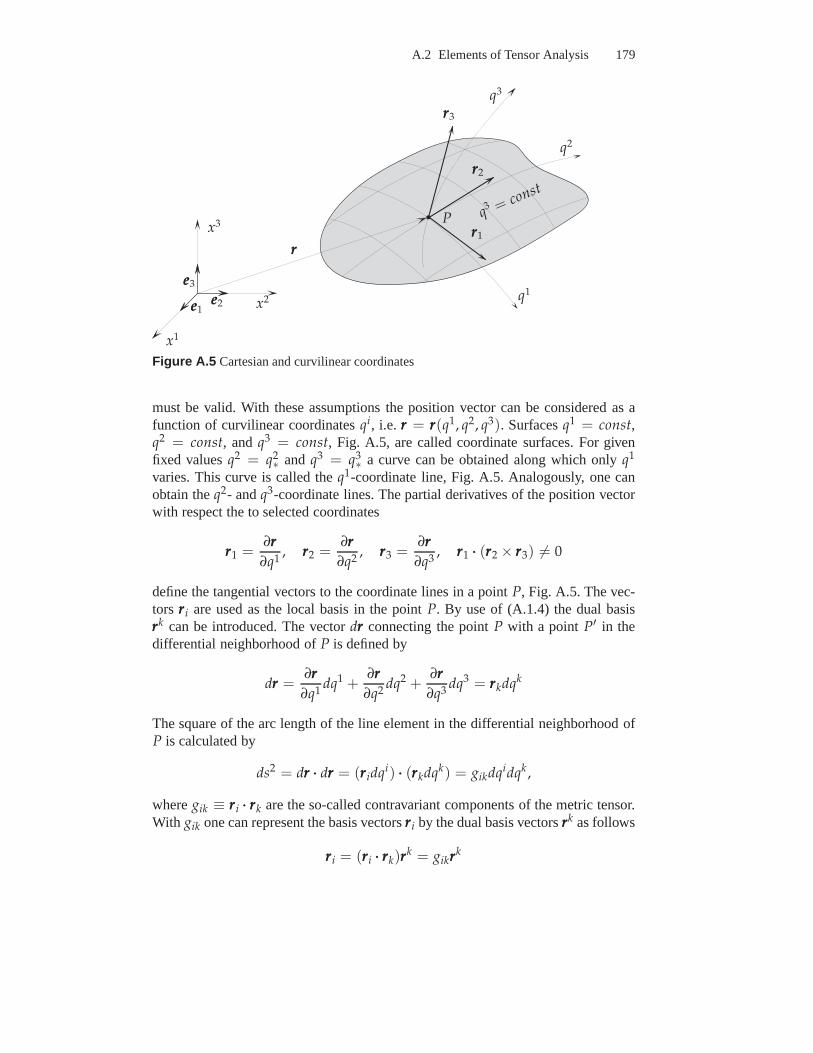
A.2 Elements of Tensor Analysis 179
eee1eee2
eee3
x2
x3
x1
rrr
q1
q2
q3
rrr1
rrr2
rrr3
P q3 = const
Figure A.5 Cartesian and curvilinear coordinates
must be valid. With these assumptions the position vector can be considered as afunction of curvilinear coordinatesqi, i.e.rrr = rrr(q1, q2, q3). Surfacesq1 = const,q2 = const, andq3 = const, Fig. A.5, are called coordinate surfaces. For givenfixed valuesq2 = q2
∗ and q3 = q3∗ a curve can be obtained along which onlyq1
varies. This curve is called theq1-coordinate line, Fig. A.5. Analogously, one canobtain theq2- andq3-coordinate lines. The partial derivatives of the positionvectorwith respect the to selected coordinates
rrr1 =∂rrr
∂q1, rrr2 =
∂rrr
∂q2, rrr3 =
∂rrr
∂q3, rrr1 ··· (rrr2 × rrr3) 6= 0
define the tangential vectors to the coordinate lines in a point P, Fig. A.5. The vec-tors rrri are used as the local basis in the pointP. By use of (A.1.4) the dual basisrrrk can be introduced. The vectordrrr connecting the pointP with a point P′ in thedifferential neighborhood ofP is defined by
drrr =∂rrr
∂q1dq1 +
∂rrr
∂q2dq2 +
∂rrr
∂q3dq3 = rrrkdqk
The square of the arc length of the line element in the differential neighborhood ofP is calculated by
ds2 = drrr ··· drrr = (rrridqi) ··· (rrrkdqk) = gikdqidqk ,
wheregik ≡ rrri ··· rrrk are the so-called contravariant components of the metric tensor.With gik one can represent the basis vectorsrrri by the dual basis vectorsrrrk as follows
rrri = (rrri ··· rrrk)rrrk = gikrrrk
180 A Some Basic Rules of Tensor Calculus
Similarlyrrri = (rrri ··· rrrk)rrrk = gikrrrk, gik ≡ rrri ··· rrrk,
wheregik are termed covariant components of the metric tensor. For the selectedbasesrrri andrrrk the second rank unit tensor has the following representations
III = rrri ⊗ rrri = rrri ⊗ gikrrrk = gikrrri ⊗ rrrk = gikrrri ⊗ rrrk = rrri ⊗ rrri
A.2.2 The Hamilton (Nabla) Operator
A scalar field is a function which assigns a scalar to each spatial point P for thedomain of definition. Let us consider a scalar fieldϕ(rrr) = ϕ(q1, q2, q3). The totaldifferential of ϕ by moving from a pointP to a pointP′ in the differential neighbor-hood is
dϕ =∂ϕ
∂q1dq1 +
∂ϕ
∂q2dq2 +
∂ϕ
∂q3dq3 =
∂ϕ
∂qkdqk
Taking into account thatdqk = drrr ··· rrrk
dϕ = drrr ··· rrrk ∂ϕ
∂qk= drrr ···∇∇∇ϕ
The vector∇∇∇ϕ is called the gradient of the scalar fieldϕ and the invariant operator∇∇∇ (the Hamilton or nabla operator) is defined by
∇∇∇ = rrrk ∂
∂qk
For a vector fieldaaa(rrr) one may write
daaa = (drrr ··· rrrk)∂aaa
∂qk= drrr ··· rrrk ⊗ ∂aaa
∂qk= drrr ···∇∇∇⊗ aaa = (∇∇∇⊗ aaa)T ··· dddrrr,
∇∇∇⊗ aaa = rrrk ⊗ ∂aaa
∂qk
The gradient of a vector field is a second rank tensor. The operation∇∇∇ can be appliedto tensors of any rank. For vectors and tensors the followingadditional operationsare defined
divaaa ≡ ∇∇∇··· aaa = rrrk ··· ∂aaa
∂qk
rotaaa ≡ ∇∇∇× aaa = rrrk × ∂aaa
∂qk
The following identities can be verified
∇∇∇⊗ rrr = rrrk ⊗ ∂rrr
∂qk= rrrk ⊗ rrrk = III, ∇∇∇ ··· rrr = 3
A.2 Elements of Tensor Analysis 181
For a scalarα, a vectoraaa and for a second rank tensorAAA the following identities arevalid
∇∇∇(αaaa) = rrrk ⊗ ∂(αaaa)
∂qk=
(
rrrk ∂α
∂qk
)
⊗ aaa + αrrrk ⊗ ∂aaa
∂qk= (∇∇∇α) ⊗ aaa + α∇∇∇⊗ aaa,
(A.2.1)
∇∇∇ ··· (AAA ··· aaa) = rrrk ··· ∂(AAA ··· aaa)
∂qk= rrrk ··· ∂AAA
∂qk··· aaa + rrrk ··· AAA ··· ∂aaa
∂qk
= (∇∇∇ ··· AAA) ··· aaa + AAA ······(
∂aaa
∂qk⊗ rrrk
)
= (∇∇∇ ··· AAA) ··· aaa + AAA ······ (∇∇∇⊗ aaa)T
(A.2.2)
Here the identity (A.1.6) is used. For a second rank tensorAAA and a position vectorrrrone can prove the following identity
∇∇∇ ··· (AAA × rrr) = rrrk ··· ∂(AAA × rrr)
∂qk= rrrk ··· ∂AAA
∂qk× rrr + rrrk ··· AAA × ∂rrr
∂qk
= (∇∇∇ ··· AAA)× rrr + rrrk ··· AAA × rrrk = (∇∇∇ ··· AAA) × rrr − AAA×(A.2.3)
Here we used the definition of the vector invariant as follows
AAA× =(
rrrk ⊗ rrrk ··· AAA)
×= rrrk × (rrrk ··· AAA) = −rrrk ··· AAA × rrrk
A.2.3 Integral Theorems
Let ϕ(rrr), aaa(rrr) andAAA(rrr) be scalar, vector and second rank tensor fields. LetV bethe volume of a bounded domain with a regular surfaceA(V) andnnn be the outerunit normal to the surface atrrr. The integral theorems can be summarized as follows
– Gradient Theorems∫
V
∇∇∇ϕ dV =∫
A(V)
nnnϕ dA,
∫
V
∇∇∇⊗ aaa dV =∫
A(V)
nnn ⊗ aaa dA,
∫
V
∇∇∇⊗ AAA dV =∫
A(V)
nnn ⊗ AAA dA
– Divergence Theorems∫
V
∇∇∇ ··· aaa dV =∫
A(V)
nnn ··· aaa dA,
∫
V
∇∇∇ ··· AAA dV =∫
A(V)
nnn · AAA dA
182 A Some Basic Rules of Tensor Calculus
– Curl Theorems∫
V
∇∇∇× aaa dV =∫
A(V)
nnn × aaa dA,
∫
V
∇∇∇× AAA dV =∫
A(V)
nnn × AAA dA
A.2.4 Scalar-Valued Functions of Vectors and SecondRank Tensors
Let ψ be a scalar valued function of a vectoraaa and a second rank tensorAAA, i.e.ψ = ψ(aaa, AAA). Introducing a basiseeei the functionψ can be represented as follows
ψ(aaa, AAA) = ψ(aieeei, Aijeeei ⊗ eeej) = ψ(ai, Aij)
The partial derivatives ofψ with respect toaaa and AAA are defined according to thefollowing rule
dψ =∂ψ
∂aidai +
∂ψ
∂AijdAij
= daaa ··· eeei ∂ψ
∂ai+ dAAA ······ eeej ⊗ eeei ∂ψ
∂AijdAij
(A.2.4)
In the coordinates-free form the above rule can be rewrittenas follows
dψ = daaa ··· ∂ψ
∂aaa+ dAAA ······
(
∂ψ
∂AAA
)T
= daaa ··· ψ,aaa + dAAA ······ (ψ,AAA)T (A.2.5)
with
ψ,aaa ≡∂ψ
∂aaa=
∂ψ
∂aieeei, ψ,AAA ≡ ∂ψ
∂AAA=
∂ψ
∂Aijeeei ⊗ eeej
One can verify thatψ,aaa andψ,AAA are independent from the choice of the basis. Onemay prove the following formulae for the derivatives of principal invariants of asecond rank tensorAAA
J1(AAA),AAA = III, J1(AAA2),AAA = 2AAAT, J1(AAA3),AAA = 3AAA2T,
J2(AAA),AAA = J1(AAA)III − AAAT, (A.2.6)
J3(AAA),AAA = AAA2T − J1(AAA)AAAT + J2(AAA)III = J3(AAA)(AAAT)−1
A.3 Orthogonal Transformations and OrthogonalInvariants
An application of the theory of tensor functions is to find a basic set of scalar invari-ants for a given group of symmetry transformations, such that each invariant relative
A.3 Orthogonal Transformations and Orthogonal Invariants183
to the same group is expressible as a single-valued functionof the basic set. The ba-sic set of invariants is called functional basis. To obtain acompact representationfor invariants, it is required that the functional basis is irreducible in the sense thatremoving any one invariant from the basis will imply that a complete representationfor all the invariants is no longer possible.
Such a problem arises in the formulation of constitutive equations for a givengroup of material symmetries. For example, the strain energy density of an elasticnon-polar material is a scalar valued function of the secondrank symmetric straintensor. In the theory of the Cosserat continuum two strain measures are introduced,where the first strain measure is the polar tensor while the second one is the axialtensor, e.g. [108]. The strain energy density of a thin elastic shell is a function oftwo second rank tensors and one vector, e.g. [25]. In all cases the problem is to finda minimum set of functionally independent invariants for the considered tensorialarguments.
For the theory of tensor functions we refer to [71]. Representations of tensorfunctions are reviewed in [280, 330]. An orthogonal transformation of a scalarα, avectoraaa and a second rank tensorAAA is defined by [25, 332]
α′ ≡ (det QQQ)ζα, aaa′ ≡ (det QQQ)ζQQQ ··· aaa, AAA′ ≡ (det QQQ)ζQQQ ··· AAA ··· QQQT, (A.3.1)
whereQQQ is an orthogonal tensor, i.e.QQQ ··· QQQT = III, detQQQ = ±1, III is the secondrank unit tensor,ζ = 0 for absolute (polar) scalars, vectors and tensors andζ = 1for axial ones. An example of the axial scalar is the mixed product of three polarvectors, i.e.α = aaa ··· (bbb× ccc). A typical example of the axial vector is the cross productof two polar vectors, i.e.ccc = aaa × bbb. An example of the second rank axial tensoris the skew-symmetric tensorWWW = aaa × III, whereaaa is a polar vector. Consider agroup of orthogonal transformationsS (e.g., the material symmetry transformations)characterized by a set of orthogonal tensorsQQQ. A scalar-valued function of a secondrank tensorf = f (AAA) is called to be an orthogonal invariant under the groupS if
∀QQQ ∈ S : f (AAA′) = (det QQQ)η f (AAA), (A.3.2)
whereη = 0 if values of f are absolute scalars andη = 1 if values of f are axialscalars.
Any second rank tensorBBB can be decomposed into the symmetric and the skew-symmetric part, i.e.BBB = AAA + aaa × III, whereAAA is the symmetric tensor andaaa is theassociated vector. Thereforef (BBB) = f (AAA, aaa). If BBB is a polar (axial) tensor, thenaaa isan axial (polar) vector. For the set of second rank tensors and vectors the definitionof an orthogonal invariant (A.3.2) can be generalized as follows
∀QQQ ∈ S : f (AAA′1, AAA′
2, . . . , AAA′n, aaa′1, aaa′2, . . . , aaa′k)
= (det QQQ)η f (AAA1, AAA2, . . . AAAn, aaa1, aaa2, . . . , aaak), AAAi = AAATi
(A.3.3)
184 A Some Basic Rules of Tensor Calculus
A.3.1 Invariants for the Full Orthogonal Group
In [335] orthogonal invariants for different sets of secondrank tensors and vectorswith respect to the full orthogonal group are presented. It is shown that orthogonalinvariants are integrals of a generic partial differentialequation (basic equations forinvariants). Let us present two following examples
– Orthogonal invariants of a symmetric second rank tensorAAA are
Ik = tr AAAk, k = 1, 2, 3
Instead ofIk it is possible to use the principal invariantsJk defined by (A.1.8).– Orthogonal invariants of a symmetric second rank tensorAAA and a vectoraaa are
Ik = tr AAAk, k = 1, 2, 3, I4 = aaa ··· aaa, I5 = aaa ··· AAA ··· aaa,I6 = aaa ··· AAA2 ··· aaa, I7 = aaa ··· AAA2 ··· (aaa × AAA ··· aaa)
(A.3.4)
In the above set of invariants only 6 are functionally independent. The relationbetween the invariants (so-called syzygy, [71]) can be formulated as follows
I27 =
∣
∣
∣
∣
∣
∣
I4 I5 I6
I5 I6 aaa ··· AAA3 ··· aaaI6 aaa ··· AAA3 ··· aaa aaa ··· AAA4 ··· aaa
∣
∣
∣
∣
∣
∣
, (A.3.5)
whereaaa ··· AAA3 ··· aaa andaaa ··· AAA4 ··· aaa can be expressed byIl , l = 1, . . . 6 applying theCayley-Hamilton theorem (A.1.7).
The set of invariants for a symmetric second rank tensorAAA and a vectoraaa can beapplied for a non-symmetric second rank tensorBBB since it can be represented byBBB = AAA + aaa × III, AAA = AAAT.
A.3.2 Invariants for the Transverse Isotropy Group
Transverse isotropy is an important type of the symmetry transformation due to avariety of applications. Transverse isotropy is usually assumed in constitutive mod-eling of fiber reinforced materials, e.g. [21], fiber suspensions, e.g. [22], direction-ally solidified alloys, e.g. [213], deep drawing sheets, e.g. [50, 57] and piezoelectricmaterials, e.g. [285]. The invariants and generating sets for tensor-valued functionswith respect to different cases of transverse isotropy are discussed in [79, 328] (seealso relevant references therein). In what follows we analyze the problem of a func-tional basis within the theory of linear first order partial differential equations ratherthan the algebra of polynomials. We develop the idea proposed in [335] for the in-variants with respect to the full orthogonal group to the case of transverse isotropy.The invariants will be found as integrals of the generic partial differential equa-tions. Although a functional basis formed by these invariants does not include anyredundant element, functional relations between them may exist. It may be there-fore useful to find out simple forms of such relations. We showthat the proposedapproach may supply results in a direct, natural manner.
A.3 Orthogonal Transformations and Orthogonal Invariants185
Invariants for a Single Second Rank Symmetric Tensor. Consider theproper orthogonal tensor which represents a rotation abouta fixed axis, i.e.
QQQ(ϕmmm) = mmm ⊗mmm + cos ϕ(III −mmm ⊗mmm) + sin ϕmmm × III, det QQQ(ϕmmm) = 1,(A.3.6)
wheremmm is assumed to be a constant unit vector (axis of rotation) andϕ denotesthe angle of rotation aboutmmm. The symmetry transformation defined by this tensorcorresponds to the transverse isotropy, whereby five different cases are possible, e.g.[299, 331]. Let us find scalar-valued functions of a second rank symmetric tensorAAAsatisfying the condition
f (AAA′(ϕ))= f (QQQ(ϕmmm) ···AAA ···QQQT(ϕmmm)) = f (AAA), AAA′(ϕ) ≡ QQQ(ϕmmm) ···AAA ···QQQT(ϕmmm)(A.3.7)
Equation (A.3.7) must be valid for any angle of rotationϕ. In (A.3.7) only the left-hand side depends onϕ. Therefore its derivative with respect toϕ can be set to zero,i.e.
d f
dϕ=
dAAA′
dϕ······(
∂ f
∂AAA′
)T
= 0 (A.3.8)
The derivative ofAAA′ with respect toϕ can be calculated by the following rules
dAAA′(ϕ) = dQQQ(ϕmmm) ··· AAA ···QQQT(ϕmmm) + QQQ(ϕmmm) ··· AAA ··· dQQQT(ϕmmm),
dQQQ(ϕmmm) = mmm ×QQQ(ϕmmm)dϕ ⇒ dQQQT(ϕmmm) = −QQQT(ϕmmm) ×mmm dϕ(A.3.9)
By inserting the above equations into (A.3.8) we obtain
(mmm × AAA − AAA ×mmm) ······(
∂ f
∂AAA
)T
= 0 (A.3.10)
Equation (A.3.10) is classified in [92] to be the linear homogeneous first order par-tial differential equation. The characteristic system of (A.3.10) is
dAAA
ds= (mmm × AAA − AAA ×mmm) (A.3.11)
Any system ofn linear ordinary differential equations has not more thenn − 1functionally independent integrals [92]. By introducing abasiseeei the tensorAAA canbe written down in the formAAA = Aijeeei ⊗ eeej and (A.3.11) is a system of six ordi-
nary differential equations with respect to the coordinates Aij. The five integrals of(A.3.11) may be written down as follows
gi(AAA) = ci, i = 1, 2, . . . , 5,
whereci are integration constants. Any function of the five integrals gi is the so-lution of the partial differential equation (A.3.10). Therefore the five integralsgi
represent the invariants of the symmetric tensorAAA with respect to the symmetrytransformation (A.3.6). The solutions of (A.3.11) are

186 A Some Basic Rules of Tensor Calculus
AAAk(s) = QQQ(smmm) ··· AAAk0 ···QQQT(smmm), k = 1, 2, 3, (A.3.12)
whereAAA0 is the initial condition. In order to find the integrals, the variables mustbe eliminated from (A.3.12). Taking into account the following identities
tr (QQQ ··· AAAk ···QQQT) = tr (QQQT ···QQQ ··· AAAk) = tr AAAk, mmm ···QQQ(smmm) = mmm,
(QQQ ··· aaa) × (QQQ ··· bbb) = (det QQQ)QQQ ··· (aaa × bbb)(A.3.13)
and using the notationQQQm ≡ QQQ(smmm) the integrals can be found as follows
tr (AAAk) = tr (AAAk0), k = 1, 2, 3,
mmm ··· AAAl ···mmm = mmm ···QQQm ··· AAAl0 ···QQQT
m ···mmm
= mmm ··· AAAl0 ···mmm, l = 1, 2,
mmm ··· AAA2 ··· (mmm × AAA ·········mmm) = mmm ···QQQTm ··· AAA2
0 ···QQQm ··· (mmm ×QQQTm ··· AAA0 ··· QQQm ···mmm)
= mmm ··· AAA20 ···QQQm ···
[
(QQQTm ···mmm) × (QQQT
m ··· AAA0 ···mmm)]
= mmm ··· AAA20 ··· (mmm × AAA0 ···mmm)
(A.3.14)As a result we can formulate the six invariants of the tensorAAA with respect to thesymmetry transformation (A.3.6) as follows
Ik = tr (AAAk), k = 1, 2, 3, I4 = mmm ··· AAA ···mmm,
I5 = mmm ··· AAA2 ···mmm, I6 = mmm ··· AAA2 ··· (mmm × AAA ·········mmm)(A.3.15)
The invariants with respect to various symmetry transformations are discussed in[79]. For the case of the transverse isotropy six invariantsare derived in [79] by theuse of another approach. In this sense our result coincides with the result givenin [79]. However, from our derivations it follows that only five invariants listedin (A.3.15) are functionally independent. Taking into account that I6 is the mixedproduct of vectorsmmm, AAA ··· mmm andAAA2 ··· mmm the relation between the invariants can bewritten down as follows
I26 = det
1 I4 I5
I4 I5 mmm ··· AAA3 ···mmmI5 mmm ··· AAA3 ···mmm mmm ··· AAA4 ···mmm
(A.3.16)
One can verify thatmmm ··· AAA3 ··· mmm and mmm ··· AAA4 ··· mmm are transversely isotropic invari-ants, too. However, applying the the Cayley-Hamilton theorem (A.1.7) they can beuniquely expressed byI1, I2, . . . I5 in the following way [54]
mmm ··· AAA3 ···mmm = J1 I5 + J2 I4 + J3,
mmm ··· AAA4 ···mmm = (J21 + J2)I5 + (J1 J2 + J3)I4 + J1 J3,
where J1, J2 and J3 are the principal invariants ofAAA defined by (A.1.8). Let usnote that the invariantI6 cannot be dropped. In order to verify this, it is enough toconsider two different tensors
A.3 Orthogonal Transformations and Orthogonal Invariants187
AAA and BBB = QQQn ··· AAA ···QQQTn ,
where
QQQn ≡ QQQ(πnnn) = 2nnn ⊗ nnn − III, nnn ··· nnn = 1, nnn ···mmm = 0, det QQQn = 1
One can prove that the tensorAAA and the tensorBBB have the same invariantsI1, I2, . . . , I5. Taking into account thatmmm ··· QQQn = −mmm and applying the last iden-tity in (A.3.13) we may write
I6(BBB) = mmm ··· BBB2 ··· (mmm × BBB ···mmm) = mmm ··· AAA2 ···QQQTn ··· (mmm ×QQQn ··· AAA ···mmm)
= −mmm ··· AAA2 ··· (mmm × AAA ···mmm) = −I6(AAA)
We observe that the only difference between the two considered tensors is the signof I6. Therefore, the triples of vectorsmmm, AAA ···mmm, AAA2 ···mmm andmmm, BBB ···mmm , BBB2 ···mmm havedifferent orientations and cannot be combined by a rotation. It should be noted thatthe functional relation (A.3.16) would in no way imply that the invariantI6 shouldbe “dependent” and hence “redundant”, namely should be removed from the basis(A.3.15). In fact, the relation (A.3.16) determines the magnitude but not the sign ofI6.
To describe yielding and failure of oriented solids a dyadMMM = vvv ⊗ vvv has beenused in [53, 75], where the vectorvvv specifies a privileged direction. A plastic po-tential is assumed to be an isotropic function of the symmetric Cauchy stress tensorand the tensor generatorMMM. Applying the representation of isotropic functions theintegrity basis including ten invariants was found. In the special casevvv = mmm thenumber of invariants reduces to the fiveI1, I2, . . . I5 defined by (A.3.15). Further de-tails of this approach and applications in continuum mechanics are given in [59, 71].However, the problem statement to find an integrity basis of asymmetric tensorAAAand a dyadMMM, i.e. to find scalar valued functionsf (AAA, MMM) satisfying the condition
f (QQQ ··· AAA ···QQQT, QQQ ··· MMM ···QQQT) = (det QQQ)η f (AAA, MMM),
∀QQQ, QQQ ···QQQT = III, det QQQ = ±1(A.3.17)
essentially differs from the problem statement (A.3.7). Inorder to show this wetake into account that the symmetry group of a dyadMMM, i.e. the set of orthogonalsolutions of the equationQQQ ··· MMM ···QQQT = MMM includes the following elements
QQQ1,2 = ±III,
QQQ3 = QQQ(ϕmmm), mmm =vvv
|vvv| ,QQQ4 = QQQ(πnnn) = 2nnn ⊗ nnn − III, nnn ··· nnn = 1, nnn ··· vvv = 0,
(A.3.18)
whereQQQ(ϕmmm) is defined by (A.3.6). The solutions of the problem (A.3.17) areautomatically the solutions of the following problem
f (QQQi ··· AAA ···QQQTi , MMM) = (det QQQi)
η f (AAA, MMM), i = 1, 2, 3, 4,
188 A Some Basic Rules of Tensor Calculus
i.e. the problem to find the invariants ofAAA relative to the symmetry group (A.3.18).However, (A.3.18) includes much more symmetry elements if compared to the prob-lem statement (A.3.7).
An alternative set of transversely isotropic invariants can be formulated by theuse of the following decomposition
AAA = αmmm ⊗mmm + β(III −mmm ⊗mmm) + AAApD + ttt ⊗mmm + mmm ⊗ ttt, (A.3.19)
whereα, β, AAApD andttt are projections ofAAA. With the projectorsPPP1 = mmm ⊗mmm andPPP2 = III −mmm ⊗mmm we may write
α = mmm ··· AAA ···mmm = tr (AAA ··· PPP1),
β =1
2(tr AAA −mmm ··· AAA ···mmm) =
1
2tr (AAA ··· PPP2),
AAApD = PPP2 ··· AAA ··· PPP2 − βPPP2,
ttt = mmm ··· AAA ··· PPP2
(A.3.20)
The decomposition (A.3.19) is the analogue to the followingrepresentation of avectoraaa
aaa = III ··· aaa = mmm ⊗mmm ··· aaa + (III −mmm ⊗mmm) ··· aaa = ψmmm + τττ, ψ = aaa ···mmm, τττ = PPP2 ··· aaa(A.3.21)
Decompositions of the type (A.3.19) are applied in [68, 79].The projections intro-duced in (A.3.20) have the following properties
tr (AAApD) = 0, AAApD ···mmm = mmm ··· AAApD = 000, ttt ···mmm = 0 (A.3.22)
With (A.3.19) and (A.3.22) the tensor equation (A.3.11) canbe transformed to thefollowing system of equations
dα
ds= 0,
dβ
ds= 0,
dAAApD
ds= mmm × AAApD − AAApD ×mmm,
dttt
ds= mmm × ttt
(A.3.23)
From the first two equations we observe thatα andβ are transversely isotropic in-variants. The third equation can be transformed to one scalar and one vector equationas follows
dAAApD
ds······ AAApD = 0 ⇒ d(AAApD ······ AAApD)
ds= 0,
dbbb
ds= mmm × bbb
with bbb ≡ AAApD ··· ttt. We observe thattr (AAA2pD) = AAApD ······ AAApD is the transversely
isotropic invariant, too. Finally, we have to find the integrals of the following system
A.3 Orthogonal Transformations and Orthogonal Invariants189
dttt
ds= ttt ×mmm,
dbbb
ds= bbb ×mmm
(A.3.24)
The solutions of (A.3.24) are
ttt(s) = QQQ(smmm) ··· ttt0, bbb(s) = QQQ(smmm) ··· bbb0,
wherettt0 andbbb0 are initial conditions. The vectorsttt andbbb belong to the plane ofisotropy, i.e.ttt ··· mmm = 0 andbbb ··· mmm = 0. Therefore, one can verify the followingintegrals
ttt ··· ttt = ttt0 ··· ttt0, bbb ··· bbb = bbb0 ··· bbb0, ttt ··· bbb = ttt0 ··· bbb0, (ttt × bbb) ···mmm = (ttt0 × bbb0) ···mmm(A.3.25)
We found seven integrals, but only five of them are functionally independent. Inorder to formulate the relation between the integrals we compute
bbb ··· bbb = ttt ··· AAA2pD ··· ttt, ttt ··· bbb = ttt ··· AAApD ··· ttt
For any plane tensorAAAp satisfying the equationsAAAp ···mmm = mmm ··· AAAp = 000 the Cayley-Hamilton theorem can be formulated as follows, see e.g. [71]
AAA2p − (tr AAAp)AAAp +
1
2
[
(tr AAAp)2 − tr (AAA2
p)]
(III −mmm ⊗mmm) = 000
Sincetr AAApD = 0 we have
2AAA2pD = tr (AAA2
pD)(III −mmm ⊗mmm), ttt ··· AAA2pD ··· ttt =
1
2tr (AAA2
pD)(ttt ··· ttt)
Becausetr (AAA2pD) andttt ··· ttt are already defined, the invariantbbb ··· bbb can be omitted.
The vectorttt × bbb is spanned on the axismmm. Therefore
ttt × bbb = γmmm, γ = (ttt × bbb) ···mmm,
γ2 = (ttt × bbb) ··· (ttt × bbb) = (ttt ··· ttt)(bbb ··· bbb)− (ttt ··· bbb)2
Now we can summarize six invariants and one relation betweenthem as follows
I1 = α, I2 = β, I3 =1
2tr (AAA2
pD), I4 = ttt ··· ttt = ttt ··· AAA ···mmm,
I5 = ttt ··· AAApD ··· ttt, I6 = (ttt × AAApD ··· ttt) ···mmm,
I26 = I2
4 I3 − I25
(A.3.26)
Let us assume that the symmetry transformationQQQn ≡ QQQ(πnnn) belongs to thesymmetry group of the transverse isotropy, as it was made in [71, 59]. In this casef (AAA′) = f (QQQn ··· AAA ···QQQT
n ) = f (AAA) must be valid. WithQQQn ···mmm = −mmm we can write
α′ = α, β′ = β, AAA′pD = AAApD, ttt′ = −QQQn ··· ttt
190 A Some Basic Rules of Tensor Calculus
Therefore in (A.3.26)I′k = Ik, k = 1, 2, . . . , 5 and
I′6 = (ttt′ × AAA′pD ··· ttt′) ···mmm =
(
(QQQn ··· ttt) ×QQQn ··· AAApD ··· ttt)
···mmm
= (ttt × AAApD ··· ttt) ··· QQQn ···mmm = −(ttt × AAApD ··· ttt) ···mmm = − I6
Consequently
f (AAA′) = f ( I′1, I′2, . . . , I′5, I′6) = f ( I1, I2, . . . , I5,− I6)
⇒ f (AAA) = f ( I1, I2, . . . , I5, I26 )
and I26 can be omitted due to the last relation in (A.3.26).
Invariants for a Set of Vectors and Second Rank Tensors. By settingQQQ = QQQ(ϕmmm) in (A.3.3) and taking the derivative of (A.3.3) with respectto ϕ resultsin the following generic partial differential equation
n
∑i=1
(
∂ f
∂AAAi
)T
······ (mmm × AAAi − AAAi ×mmm) +k
∑j=1
∂ f
∂aaaj··· (mmm × aaaj) = 0 (A.3.27)
The characteristic system of (A.3.27) is
dAAAi
ds= (mmm × AAAi − AAAi ×mmm), i = 1, 2, . . . , n,
daaaj
ds= mmm × aaaj, j = 1, 2, . . . , k
(A.3.28)
The above system is a system ofN ordinary differential equations, whereN = 6n +3k is the total number of coordinates ofAAAi andaaaj for a selected basis. The system(A.3.28) has not more thenN − 1 functionally independent integrals. Therefore wecan formulate:
Theorem A.3.1. A set of n symmetric second rank tensors and k vectors withN = 6n + 3k independent coordinates for a given basis has not more than N − 1functionally independent invariants for N > 1 and one invariant for N = 1 withrespect to the symmetry transformation QQQ(ϕmmm).
In essence, the proof of this theorem is given within the theory of linear first orderpartial differential equations [92].
As an example let us consider the set of a symmetric second rank tensorAAA anda vectoraaa. This set has eight independent invariants. For a visual perception it isuseful to keep in mind that the considered set is equivalent to
AAA, aaa, AAA ··· aaa, AAA2 ··· aaa
Therefore it is necessary to find the list of invariants, whose fixation determines thisset as a rigid whole. The generic equation (A.3.27) takes theform
(
∂ f
∂AAA
)T
······ (mmm × AAA − AAA ×mmm) +∂ f
∂aaa··· (mmm × aaa) = 0 (A.3.29)
A.3 Orthogonal Transformations and Orthogonal Invariants191
The characteristic system of (A.3.29) is
dAAA
ds= mmm × AAA − AAA ×mmm,
daaa
ds= mmm × aaa (A.3.30)
This system of ninth order has eight independent integrals.Six of them are invariantsof AAA andaaa with respect to the full orthogonal group. They fix the considered set asa rigid whole. The orthogonal invariants are defined by Eqs (A.3.4) and (A.3.5).
Let us note that the invariantI7 in (A.3.4) cannot be ignored. To verify this it isenough to consider two different sets
AAA, aaa and BBB = QQQp ··· AAA ···QQQTp , aaa,
whereQQQp = III − 2ppp ⊗ ppp, ppp ··· ppp = 1, ppp ··· aaa = 0. One can prove that the invariantsI1, I2, . . . , I6 are the same for these two sets. The only difference is the invariant I7,i.e.aaa ···BBB2 ··· (aaa × BBB ··· aaa) = −aaa ···AAA2 ··· (aaa × AAA ··· aaa) Therefore the triples of vectorsaaa, AAA ···aaa, AAA2 ··· aaa andaaa, BBB ··· aaa, BBB2 ··· aaa have different orientations and cannot be combined bya rotation. In order to fix the considered set with respect to the unit vectormmm it isenough to fix the next two invariants
I8 = mmm ··· AAA ···mmm, I9 = mmm ··· aaa (A.3.31)
The eight independent transversely isotropic invariants are (A.3.4), (A.3.5) and(A.3.31).
A.3.3 Invariants for the Orthotropic Symmetry Group
Consider orthogonal tensorsQQQ1 = III − 2nnn1 ⊗ nnn1 and QQQ2 = III − 2nnn2 ⊗ nnn2,det QQQ1 = det QQQ2 = −1. These tensors represent the mirror reflections, wherebythe unit orthogonal vectors±nnn1 and±nnn2, are the normal directions to the mirrorplanes. The above tensors are the symmetry elements of the orthotropic symmetrygroup. The invariants must be found from
f (QQQ1 ··· AAA ···QQQT1 ) = f (QQQ2 ··· AAA ···QQQT
2 ) = f (AAA)
Consequently,
f (QQQ1 ··· QQQ2 ··· AAA ···QQQT2 ···QQQT
1 ) = f (QQQ1 ··· AAA ···QQQT1 ) = f (QQQ2 ··· AAA ···QQQT
2 ) = f (AAA)
and the tensorQQQ3 = QQQ1 ···QQQ2 = 222n3 ⊗nnn3 − III belongs to the symmetry group, wherethe unit vectornnn3 is orthogonal tonnn1 andnnn2. Taking into account thatQQQi ···nnni = −nnni
(no summation convention),QQQi ··· nnnj = nnnj, i 6= j and using the notationAAA′i =
QQQi ··· AAA ···QQQTi we can write
tr (AAA′k) = tr (AAAk), k = 1, . . . , 3, i = 1, 2, 3
nnni ··· AAA′ ··· nnni = nnni ···QQQi ··· AAA ··· QQQTi ··· nnni
= nnni ··· AAA ··· nnni, i = 1, 2, 3
nnni ··· AAA′2 ··· nnni = nnni ···QQQi ··· AAA2 ···QQQTi ··· nnni
= nnni ··· AAA2 ··· nnni, i = 1, 2, 3
(A.3.32)

192 A Some Basic Rules of Tensor Calculus
The above set of includes 9 scalars. The number of independent scalars is 7 due tothe obvious relations
tr (AAAk) = nnn1 ··· AAAk ··· nnn1 + nnn2 ··· AAAk ··· nnn2 + nnn3 ··· AAAk ··· nnn3, k = 1, 2, 3
References
1. Abe, F. (2001): Creep rates and strengthening mechanismsin tungsten-strengthened 9Crsteels. Materials Science and EngineeringA319-A321, 770–773
2. Altenbach, H. (1999): Classical and nonclassical creep models. In: Altenbach, H.,Skrzypek, J. (eds.) Creep and Damage in Materials and Structures. Springer, Wien, NewYork, pp. 45 – 95. CISM Lecture Notes No. 399
3. Altenbach, H. (2001): A generalized limit criterion withapplication to strength, yield-ing, and damage of isotropic materials. In: Lemaitre, J. (ed.) Handbook of MaterialsBehaviour Models. Academic Press, San Diego, pp. 175 – 186
4. Altenbach, H., Altenbach, J., Kissing, W. (2004): Mechanics of composite structural el-ements. Springer, Berlin et al.
5. Altenbach, H., Altenbach, J., Naumenko, K. (1997): On theprediction of creep damageby bending of thin–walled structures. Mechanics of Time Dependent Materials1, 181–193
6. Altenbach, H., Altenbach, J., Naumenko, K. (1998): EbeneFlachentragwerke. Springer,Berlin et al.
7. Altenbach, H., Altenbach, J., Rikards, R. (1996): Einfuhrung in die Mechanik derLaminat- und Sandwichtragwerke. Deutscher Verlag fur Grundstoffindustrie, Stuttgart
8. Altenbach, H., Altenbach, J., Schieße, P. (1990): Konzepte der Schadigungsmechanikund ihre Anwendung bei der werkstoffmechanischen Bauteilanalyse. TechnischeMechanik11, 2, 81 – 93
9. Altenbach, H., Altenbach, J., Zolochevsky, A. (1995): Erweiterte Deformationsmodelleund Versagenskriterien der Werkstoffmechanik. DeutscherVerlag fur Grundstoffindus-trie, Stuttgart
10. Altenbach, H., Blumenauer, H. (1989): Grundlagen und Anwendungen der Schadi-gungsmechanik. Neue Hutte34, 6, 214 – 219
11. Altenbach, H., Breslavsky, D., Morachkovsky, O., Naumenko, K. (2000): Cyclic creepdamage in thin-walled structures. J. Strain Anal.35, 1, 1 – 11
12. Altenbach, H., Huang, C., Naumenko, K. (2001): Modelling of creep damage underthe reversed stress states considering damage activation and deactivation. TechnischeMechanik21, 4, 273 – 282
13. Altenbach, H., Huang, C., Naumenko, K. (2002): Creep damage predictions in thin-walled structures by use of isotropic and anisotropic damage models. J. Strain Anal.37,3, 265 – 275
14. Altenbach, H., Kolarow, G., Morachkovsky, O., Naumenko, K. (2000): On the accuracyof creep-damage predictions in thinwalled structures using the finite element method.Comp. Mech.25, 87 – 98
15. Altenbach, H., Kolarow, G., Naumenko, K. (1999): Solution of creep-damage problemsfor beams and rectangular plates using the Ritz and finite element method. TechnischeMechanik19, 249 – 258
194 References
16. Altenbach, H., Kushnevsky, V., Naumenko, K. (2001): On the use of solid- and shell-type finite elements in creep-damage predictions of thinwalled structures. Arch. Appl.Mech.71, 164 – 181
17. Altenbach, H., Morachkovsky, O., Naumenko, K., Sichov,A. (1996): Zum Kriechendunner Rotationsschalen unter Einbeziehung geometrischer Nichtlinearitat sowie derAsymmetrie der Werkstoffeigenschaften. Forschung im Ingenieurwesen62, 6, 47 – 57
18. Altenbach, H., Morachkovsky, O., Naumenko, K., Sychov,A. (1997): Geometricallynonlinear bending of thin-walled shells and plates under creep-damage conditions. Arch.Appl. Mech.67, 339 – 352
19. Altenbach, H., Naumenko, K. (1997): Creep bending of thin-walled shells and plates byconsideration of finite deflections. Comp. Mech.19, 490 – 495
20. Altenbach, H., Naumenko, K. (2002): Shear correction factors in creep-damage analysisof beams, plates and shells. JSME Int. J. Series A45, 77–83
21. Altenbach, H., Naumenko, K., L’vov, G.I., Pylypenko, S.(2003): Numerical estimationof the elastic properties of thin-walled structures manufactured from short-fiber rein-forced thermoplastics. Mechanics of Composite Materials39, 221–234
22. Altenbach, H., Naumenko, K., Zhilin, P. (2003): A micro-polar theory for binary mediawith application to phase-transitional flow of fiber suspensions. Continuum Mechanicsand Thermodynamics15, 539–570
23. Altenbach, H., Naumenko, K., Zhilin, P.A. (2005): A direct approach to the formulationof constitutive equations for rods and shells. In: Pietraszkiewicz, W., Szymczak, C. (eds.)Shell Structures: Theory and Applications. Taylor & Francis, Leiden, pp. 87 – 90
24. Altenbach, H., Schieße, P., Zolochevsky, A. (1991): ZumKriechen isotroper Werkstoffemit komplizierten Eigenschaften. Rheol. Acta30, 388 – 399
25. Altenbach, H., Zhilin, P.A. (1988): Osnovnye uravneniya neklassicheskoi teorii uprugikhobolochek (Basic equations of a non-classical theory of elastic shells, in Russ.). Advancesin Mechanics11, 107–148
26. Altenbach, H., Zhilin, P.A. (2004): The theory of simpleelastic shells. In: Kienzler,R., Altenbach, H., Ott, I. (eds.) Theories of Plates and Shells. Critical Review and NewApplications. Springer, Berlin et al., pp. 1 – 12
27. Altenbach, H., Zolochevsky, A. (1996): A generalized failure criterion for three-dimen-sional behaviour of isotropic materials. Engng Fracture Mechanics54, 1, 75 – 90
28. Altenbach, H., Zolochevsky, A.A. (1994): Eine energetische Variante der Theorie desKriechens und der Langzeitfestigkeit fur isotrope Werkstoffe mit komplizierten Eigen-schaften. ZAMM74, 3, 189 – 199
29. Altenbach, J., Altenbach, H. (1994): Einfuhrung in dieKontinuumsmechanik. TeubnerStudienbucher Mechanik. Teubner, Stuttgart
30. Altenbach, J., Altenbach, H., Naumenko, K. (1997): Lebensdauerabschatzungdunnwandiger Flachentragwerke auf der Grundlage phanomenologischer Materialmod-elle fur Kriechen und Schadigung. Technische Mechanik17, 4, 353 – 364
31. Altenbach, J., Altenbach, H., Naumenko, K. (2004): Egdeeffects in moderately thickplates under creep damage conditions. Technische Mechanik24, 3-4, 254 – 263
32. Antman, S. (1995): Nonlinear Problems of Elasticity. Springer, Berlin et al.33. Ashby, M.F., Gandhi, C., Taplin, D.M.R. (1979): Fracture-mechanism maps and their
construction for f.c.c. metals and alloys. Acta Metall.27, 699 – 72934. Aurich, D., Kloos, K.H., Lange, G., Macherauch, E. (1999): Eigenspannungen und
Verzug durch Warmeeinwirkung, DFG Forschungsbericht. Wiley-VCH, Weinheim etal.
35. Backhaus, G. (1983): Deformationsgesetze. Akademie-Verlag, Berlin36. Bassani, J.L., Hawk, D.E. (1990): Influence of damage on crack-tip fields under small-
scale-creep conditions. Int. J. Fracture42, 157 – 17237. Bathe, K.J. (1990): Finite-Element-Methoden. Springer-Verlag, Berlin et al.
References 195
38. Becker, A.A., Hyde, T.H., Sun, W., Andersson, P. (2002):Benchmarks for finite elementanalysis of creep continuum damage mechanics. Computational Materials Science25,34 – 41
39. Becker, A.A., Hyde, T.H., Xia, L. (1994): Numerical analysis of creep in components. J.Strain Anal.29, 3, 185 – 192
40. Bellmann, R. (1970): Introduction to Matrix Analysis. McGraw Hill, New York41. Bend Tech Inc. (2005). Induction pipe bending, standardbend tolerances. World Wide
Web page, http://www.bendtec.com/bendtol.html42. Bernhardi, O., Mucke, R. (2000): A lifetime predictionprocedure for anisotropic mate-
rials. Commmunications in Numerical Methods in Engineering 16, 519 – 52743. Bernhardt, E.O., Hanemann, H. (1938):Uber den Kriechvorgang bei dynamischer Be-
lastung und den Begriff der dynamischen Kriechfestigkeit.Z. fur Metallkunde30, 12,401 – 409
44. Bertram, A. (1989): Axiomatische Einfuhrung in die Kontinuumsmechanik. B.I. Wis-senschaftsverlag, Mannheim
45. Bertram, A. (2003): Finite thermoplasticity based on isomorphismus. Int. J. of Plasticity19, 2027 – 2050
46. Bertram, A. (2005): Elasticity nad Plasticity of Large Deformations. Springer, Berlin etal.
47. Bertram, A., Olschewski, J. (1996): Anisotropic modelling of the single crystal superal-loy SRR99. Comp. Mat. Sci.5, 12 – 16
48. Bertram, A., Olschewski, J. (2001): A phenomenologicalanisotropic creep model forcubic single crystals. In: Lemaitre, J. (ed.) Handbook of material models. AcademicPress, San Diego, pp. 303–307
49. Besseling, J.F., van der Giessen, E. (1994): Mathematical Modelling of Inelastic Defor-mation. Chapman & Hall, London et al.
50. Betten, J. (1976): Plastic anisotropy and Bauschinger-Effect - general formulation andcomparison with experimental yield curves. Acta Mechanica25, 1-2, 79 – 94
51. Betten, J. (1982): Zur Aufstellung einer Integritatsbasis fur Tensoren zweiter und vierterStufe. ZAMM 62, 5, T 274 – T 275
52. Betten, J. (1984): Materialgleichungen zur Beschreibung des sekundaren und tertiarenKriechverhaltens anisotroper Stoffe. ZAMM64, 211 – 220
53. Betten, J. (1985): On the representation of the plastic potential of anisotropic solids. In:Boehler, J.P. (ed.) Plastic Behavior of Anisotropic Solids. CNRS, Paris, pp. 213 – 228
54. Betten, J. (1987): Tensorrechnung fur Ingenieure. Springer, Berlin et al.55. Betten, J. (1993): Kontinuumsmechanik. Springer, Berlin et al.56. Betten, J. (1998): Anwendungen von Tensorfunktionen inder Kontinuumsmechanik
anisotroper Materialien. ZAMM78, 8, 507 – 52157. Betten, J. (2001): Kontinuumsmechanik. Springer, Berlin et al.58. Betten, J. (2002): Creep Mechanics. Springer, Berlin etal.59. Betten, J. (2005): Creep Mechanics. Springer, Berlin etal.60. Betten, J., Borrmann, M. (1987): Stationares Kriechverhalten innendruckbelasteter
dunnwandiger Kreiszylinderschalen unter Berucksichtigung des orthotropen Werkstoff-verhaltens und des CSD–Effektes. Forschung im Ingenieurwesen53, 3, 75 – 82
61. Betten, J., Borrmann, M., Butters, T. (1989): Materialgleichungen zur Beschreibungdes primaren Kriechverhaltens innendruckbeanspruchterZylinderschalen aus isotropemWerkstoff. Ingenieur-Archiv60, 3, 99 – 109
62. Betten, J., Butters, T. (1990): Rotationssymmetrisches Kriechbeulen dunnwandigerKreiszylinderschalen im primaren Kriechbereich. Forschung im Ingenieurwesen56, 3,84 – 89
63. Betten, J., El-Magd, E., Meydanli, S.C., Palmen, P. (1995): Untersuchnung desanisotropen Kriechverhaltens vorgeschadigter Werkstoffe am austenitischen StahlX8CrNiMoNb 1616. Arch. Appl. Mech.65, 121 – 132
196 References
64. Bialkiewicz, J., Kuna, H. (1996): Shear effect in rupture mechanics of middle-thick platesplates. Eng. Fracture Mech.54, 3, 361 – 370
65. Bielski, J., Skrzypek, J. (1989): Failure modes of elastic-plastic curved tubes under ex-ternal pressure with in-plane bending. Int. J. Mech. Sci.31, 435 – 458
66. Billington, E.W. (1985): The Poynting-Swift effect in relation to initial and post-yielddeformation. Int. J. Solids and Structures21, 4, 355 – 372
67. Billington, E.W. (1986): Introduction to the Mechanicsand Physics of Solids. Hilger,Bristol et al.
68. Bischoff-Beiermann, B., Bruhns, O. (1994): A physically motivated set of invariants andtensor generators in the case of transverse isotropy. Int. J. Eng. Sci.32, 1531 – 1552
69. Bodnar, A., Chrzanowski, M. (1991): A non-unilateral damage in creeping plates. In:Zyczkowski, M. (ed.) Creep in Structures. Springer, Berlin, Heidelberg, pp. 287 – 293
70. Bodnar, A., Chrzanowski, M. (2001): Cracking of creeping structures described bymeans of CDM. In: Murakami, S., Ohno, N. (eds.) IUTAM Symposium on Creep inStructures. Kluwer, Dordrecht, pp. 189 – 196
71. Boehler, J.P. (ed.) (1987): Application of Tensor Functions in Solid Mechanics. Springer,Wien et al.
72. Boehler, J.P. (1987): On a rational formulation of isotropic and anisotropic hardening. In:Boehler, J.P. (ed.) Applications of tensor functions in solid mechanics. Springer, Wien etal., pp. 99–122
73. Boehler, J.P. (1987): Representations for isotropic and anisotropic non-polynomial tensorfunctions. In: Boehler, J.P. (ed.) Applications of tensor functions in solid mechanics.Springer, Wien et al., pp. 31–53
74. Boehler, J.P. (1987): Yielding and failure of transversely isotropic solids. In: Boehler,J.P. (ed.) Applications of tensor functions in solid mechanics. Springer, Wien et al., pp.67–97
75. Boehler, J.P., Sawczuk, A. (1977): On yielding of oriented solids. Acta Mechanica27,185 – 206
76. Bohlke, T. (2000): Crystallographic Texture Evolution and Elastic Anisotropy. Simula-tion, Modelling and Applications, PhD-Thesis. Shaker Verlag, Aachen
77. Boyle, J.T., Spence, J. (1983): Stress Analysis for Creep. Butterworth, London78. Brebbia, C.A., Telles, J.C.T., Wrobel, L.C. (1983): Boundary Element Techniques.
Springer, Berlin79. Bruhns, O., Xiao, H., Meyers, A. (1999): On representation of yield functions for crys-
tals, quasicrystals and transversely isotropic solids. Eur. J. Mech. A/Solids18, 47 – 6780. Burlakov, A.V., Lvov, G.I., Morachkovsky, O.K. (1977):Polzuchest’ tonkikh obolochek
(Creep of thin shells, in Russ.). Kharkov State Univ. Publ.,Kharkov81. Burlakov, A.V., Lvov, G.I., Morachkovsky, O.K. (1981):Dlitel’naya prochnost’
obolochek (Long-term strength of shells, in Russ.). Vyshcha shkola, Kharkov82. Byrne, T.P., Mackenzie, A.C. (1966): Secondary creep ofa cylindrical thin shell subject
to axisymmetric loading. J. Mech. Eng. Sci.8, 2, 215 – 22583. Cane, B.J. (1981): Creep fracture of dispersion strengthened low alloy ferritic steels.
Acta Metall.29, 1581 – 159184. Cazacu, O., Barlat, F. (2003): Application of the theoryof representation to describe
yielding of anisotropic aluminium alloys. Int. J. of Eng. Sci. 41, 1367 – 138585. Chaboche, J.L. (1988): Continuum damage mechanics: part I - general concepts. Trans.
of ASME. J. Appl. Mech.55, 59 – 6486. Chaboche, J.L. (1988): Continuum damage mechanics: part II - damage growth, crack
initiation, and crack growth. Trans. of ASME. J. Appl. Mech.55, 65 – 7187. Chaboche, J.L. (1989): Constitutive equations for cyclic plasticity and cyclic viscoplas-
ticity. Int. J. Plasticity5, 247 – 302
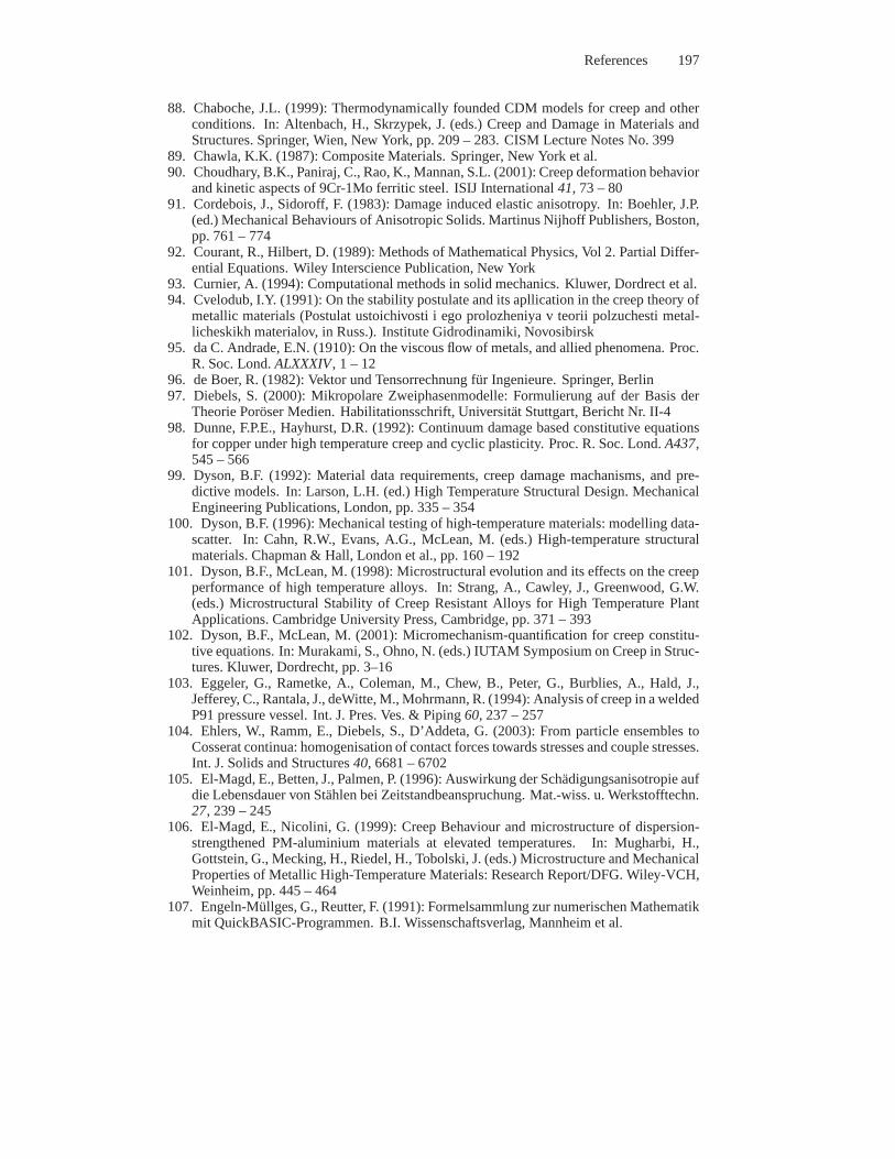
References 197
88. Chaboche, J.L. (1999): Thermodynamically founded CDM models for creep and otherconditions. In: Altenbach, H., Skrzypek, J. (eds.) Creep and Damage in Materials andStructures. Springer, Wien, New York, pp. 209 – 283. CISM Lecture Notes No. 399
89. Chawla, K.K. (1987): Composite Materials. Springer, New York et al.90. Choudhary, B.K., Paniraj, C., Rao, K., Mannan, S.L. (2001): Creep deformation behavior
and kinetic aspects of 9Cr-1Mo ferritic steel. ISIJ International 41, 73 – 8091. Cordebois, J., Sidoroff, F. (1983): Damage induced elastic anisotropy. In: Boehler, J.P.
(ed.) Mechanical Behaviours of Anisotropic Solids. Martinus Nijhoff Publishers, Boston,pp. 761 – 774
92. Courant, R., Hilbert, D. (1989): Methods of Mathematical Physics, Vol 2. Partial Differ-ential Equations. Wiley Interscience Publication, New York
93. Curnier, A. (1994): Computational methods in solid mechanics. Kluwer, Dordrect et al.94. Cvelodub, I.Y. (1991): On the stability postulate and its apllication in the creep theory of
metallic materials (Postulat ustoichivosti i ego prolozheniya v teorii polzuchesti metal-licheskikh materialov, in Russ.). Institute Gidrodinamiki, Novosibirsk
95. da C. Andrade, E.N. (1910): On the viscous flow of metals, and allied phenomena. Proc.R. Soc. Lond.ALXXXIV, 1 – 12
96. de Boer, R. (1982): Vektor und Tensorrechnung fur Ingenieure. Springer, Berlin97. Diebels, S. (2000): Mikropolare Zweiphasenmodelle: Formulierung auf der Basis der
Theorie Poroser Medien. Habilitationsschrift, Universitat Stuttgart, Bericht Nr. II-498. Dunne, F.P.E., Hayhurst, D.R. (1992): Continuum damagebased constitutive equations
for copper under high temperature creep and cyclic plasticity. Proc. R. Soc. Lond.A437,545 – 566
99. Dyson, B.F. (1992): Material data requirements, creep damage machanisms, and pre-dictive models. In: Larson, L.H. (ed.) High Temperature Structural Design. MechanicalEngineering Publications, London, pp. 335 – 354
100. Dyson, B.F. (1996): Mechanical testing of high-temperature materials: modelling data-scatter. In: Cahn, R.W., Evans, A.G., McLean, M. (eds.) High-temperature structuralmaterials. Chapman & Hall, London et al., pp. 160 – 192
101. Dyson, B.F., McLean, M. (1998): Microstructural evolution and its effects on the creepperformance of high temperature alloys. In: Strang, A., Cawley, J., Greenwood, G.W.(eds.) Microstructural Stability of Creep Resistant Alloys for High Temperature PlantApplications. Cambridge University Press, Cambridge, pp.371 – 393
102. Dyson, B.F., McLean, M. (2001): Micromechanism-quantification for creep constitu-tive equations. In: Murakami, S., Ohno, N. (eds.) IUTAM Symposium on Creep in Struc-tures. Kluwer, Dordrecht, pp. 3–16
103. Eggeler, G., Rametke, A., Coleman, M., Chew, B., Peter,G., Burblies, A., Hald, J.,Jefferey, C., Rantala, J., deWitte, M., Mohrmann, R. (1994): Analysis of creep in a weldedP91 pressure vessel. Int. J. Pres. Ves. & Piping60, 237 – 257
104. Ehlers, W., Ramm, E., Diebels, S., D’Addeta, G. (2003):From particle ensembles toCosserat continua: homogenisation of contact forces towards stresses and couple stresses.Int. J. Solids and Structures40, 6681 – 6702
105. El-Magd, E., Betten, J., Palmen, P. (1996): Auswirkungder Schadigungsanisotropie aufdie Lebensdauer von Stahlen bei Zeitstandbeanspruchung.Mat.-wiss. u. Werkstofftechn.27, 239 – 245
106. El-Magd, E., Nicolini, G. (1999): Creep Behaviour and microstructure of dispersion-strengthened PM-aluminium materials at elevated temperatures. In: Mugharbi, H.,Gottstein, G., Mecking, H., Riedel, H., Tobolski, J. (eds.)Microstructure and MechanicalProperties of Metallic High-Temperature Materials: Research Report/DFG. Wiley-VCH,Weinheim, pp. 445 – 464
107. Engeln-Mullges, G., Reutter, F. (1991): Formelsammlung zur numerischen Mathematikmit QuickBASIC-Programmen. B.I. Wissenschaftsverlag, Mannheim et al.
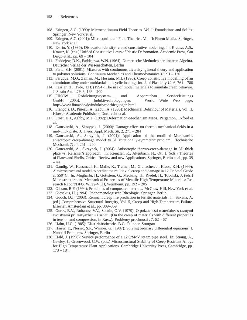
198 References
108. Eringen, A.C. (1999): Microcontinuum Field Theories.Vol. I: Foundations and Solids.Springer, New York et al.
109. Eringen, A.C. (2001): Microcontinuum Field Theories.Vol. II: Fluent Media. Springer,New York et al.
110. Estrin, Y. (1996): Dislocation-density-related constitutive modelling. In: Krausz, A.S.,Krausz, K. (eds.) Unified Constitutive Laws of Plastic Deformation. Academic Press, SanDiego et al., pp. 69 – 104
111. Faddejew, D.K., Faddejewa, W.N. (1964): Numerische Methoden der linearen Algebra.Deutscher Verlag der Wissenschaften, Berlin
112. Faria, S.H. (2001): Mixtures with continuous diversity: general theory and applicationto polymer solutions. Continuum Mechanics and Thermodynamics 13, 91 – 120
113. Faruque, M.O., Zaman, M., Hossain, M.I. (1996): Creep constitutive modelling of analuminium alloy under multiaxial and cyclic loading. Int. J. of Plasticity12, 6, 761 – 780
114. Fessler, H., Hyde, T.H. (1994): The use of model materials to simulate creep behavior.J. Strain Anal.29, 3, 193 – 200
115. FINOW Rohrleitungssystem- und Apparatebau ServiceleistungsGmbH (2005). Induktivrohrbiegungen. World Wide Web page,http://www.finow.de/de/induktivrohrbiegungen.html
116. Francois, D., Pineau, A., Zaoui, A. (1998): Mechanical Behaviour of Materials, Vol. II.Kluwer Academic Publishers, Dordrecht et al.
117. Frost, H.J., Ashby, M.F. (1982): Deformation-Mechanism Maps. Pergamon, Oxford etal.
118. Ganczarski, A., Skrzypek, J. (2000): Damage effect on thermo-mechanical fields in amid-thick plate. J. Theor. Appl. Mech.38, 2, 271 – 284
119. Ganczarski, A., Skrzypek, J. (2001): Application of the modified Murakami’sanisotropic creep-damage model to 3D rotationally-symmetric problem. TechnischeMechanik21, 4, 251 – 260
120. Ganczarski, A., Skrzypek, J. (2004): Anisotropic thermo-creep-damage in 3D thickplate vs. Reissner’s approach. In: Kienzler, R., Altenbach, H., Ott, I. (eds.) Theoriesof Plates and Shells. Critical Review and new Applications.Springer, Berlin et al., pp. 39– 44
121. Gaudig, W., Kussmaul, K., Maile, K., Tramer, M., Granacher, J., Kloos, K.H. (1999):A microstructural model to predict the multiaxial creep anddamage in 12 Cr Steel Gradeat 550C. In: Mugharbi, H., Gottstein, G., Mecking, H., Riedel, H.,Tobolski, J. (eds.)Microstructure and Mechanical Properties of Metallic High-Temperature Materials: Re-search Report/DFG. Wiley-VCH, Weinheim, pp. 192 – 205
122. Gibson, R.F. (1994): Principles of composite materials. McGraw-Hill, New York et al.123. Giesekus, H. (1994): Phanomenologische Rheologie. Springer, Berlin124. Gooch, D.J. (2003): Remnant creep life prediction in ferritic materials. In: Saxena, A.
(ed.) Comprehensive Structural Integrity, Vol. 5, Creep and High-Temperature Failure.Elsevier, Amsterdam et al., pp. 309–359
125. Gorev, B.V., Rubanov, V.V., Sosnin, O.V. (1979): O polzuchesti materialov s raznymisvoistvami pri rastyazhenii i szhatii (On the creep of materials with different propertiesin tension and compression, in Russ.). Problemy prochnosti, 7, 62 – 67
126. Hahn, H.G. (1985): Elastizitatstheorie. B.G. Teubner, Stuttgart127. Hairer, E., Norset, S.P., Wanner, G. (1987): Solving ordinary differential equations, I.
Nonstiff Problems. Springer, Berlin128. Hald, J. (1998): Service performance of a 12CrMoV steampipe steel. In: Strang, A.,
Cawley, J., Greenwood, G.W. (eds.) Microstructural Stability of Creep Resistant Alloysfor High Temperature Plant Applications. Cambridge University Press, Cambridge, pp.173 – 184
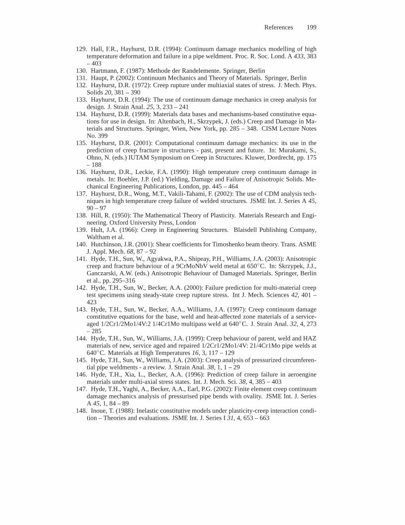
References 199
129. Hall, F.R., Hayhurst, D.R. (1994): Continuum damage mechanics modelling of hightemperature deformation and failure in a pipe weldment. Proc. R. Soc. Lond. A433, 383– 403
130. Hartmann, F. (1987): Methode der Randelemente. Springer, Berlin131. Haupt, P. (2002): Continuum Mechanics and Theory of Materials. Springer, Berlin132. Hayhurst, D.R. (1972): Creep rupture under multiaxialstates of stress. J. Mech. Phys.
Solids20, 381 – 390133. Hayhurst, D.R. (1994): The use of continuum damage mechanics in creep analysis for
design. J. Strain Anal.25, 3, 233 – 241134. Hayhurst, D.R. (1999): Materials data bases and mechanisms-based constitutive equa-
tions for use in design. In: Altenbach, H., Skrzypek, J. (eds.) Creep and Damage in Ma-terials and Structures. Springer, Wien, New York, pp. 285 – 348. CISM Lecture NotesNo. 399
135. Hayhurst, D.R. (2001): Computational continuum damage mechanics: its use in theprediction of creep fracture in structures - past, present and future. In: Murakami, S.,Ohno, N. (eds.) IUTAM Symposium on Creep in Structures. Kluwer, Dordrecht, pp. 175– 188
136. Hayhurst, D.R., Leckie, F.A. (1990): High temperaturecreep continuum damage inmetals. In: Boehler, J.P. (ed.) Yielding, Damage and Failure of Anisotropic Solids. Me-chanical Engineering Publications, London, pp. 445 – 464
137. Hayhurst, D.R., Wong, M.T., Vakili-Tahami, F. (2002):The use of CDM analysis tech-niques in high temperature creep failure of welded structures. JSME Int. J. Series A45,90 – 97
138. Hill, R. (1950): The Mathematical Theory of Plasticity. Materials Research and Engi-neering. Oxford University Press, London
139. Hult, J.A. (1966): Creep in Engineering Structures. Blaisdell Publishing Company,Waltham et al.
140. Hutchinson, J.R. (2001): Shear coefficients for Timoshenko beam theory. Trans. ASMEJ. Appl. Mech.68, 87 – 92
141. Hyde, T.H., Sun, W., Agyakwa, P.A., Shipeay, P.H., Williams, J.A. (2003): Anisotropiccreep and fracture behaviour of a 9CrMoNbV weld metal at 650C. In: Skrzypek, J.J.,Ganczarski, A.W. (eds.) Anisotropic Behaviour of Damaged Materials. Springer, Berlinet al., pp. 295–316
142. Hyde, T.H., Sun, W., Becker, A.A. (2000): Failure prediction for multi-material creeptest specimens using steady-state creep rupture stress. Int J. Mech. Sciences42, 401 –423
143. Hyde, T.H., Sun, W., Becker, A.A., Williams, J.A. (1997): Creep continuum damageconstitutive equations for the base, weld and heat-affected zone materials of a service-aged 1/2Cr1/2Mo1/4V:2 1/4Cr1Mo multipass weld at 640C. J. Strain Anal.32, 4, 273– 285
144. Hyde, T.H., Sun, W., Williams, J.A. (1999): Creep behaviour of parent, weld and HAZmaterials of new, service aged and repaired 1/2Cr1/2Mo1/4V: 21/4Cr1Mo pipe welds at640C. Materials at High Temperatures16, 3, 117 – 129
145. Hyde, T.H., Sun, W., Williams, J.A. (2003): Creep analysis of pressurized circumferen-tial pipe weldments - a review. J. Strain Anal.38, 1, 1 – 29
146. Hyde, T.H., Xia, L., Becker, A.A. (1996): Prediction ofcreep failure in aeroenginematerials under multi-axial stress states. Int. J. Mech. Sci. 38, 4, 385 – 403
147. Hyde, T.H., Yaghi, A., Becker, A.A., Earl, P.G. (2002):Finite element creep continuumdamage mechanics analysis of pressurised pipe bends with ovality. JSME Int. J. SeriesA 45, 1, 84 – 89
148. Inoue, T. (1988): Inelastic constitutive models underplasticity-creep interaction condi-tion – Theories and evaluations. JSME Int. J. Series I31, 4, 653 – 663
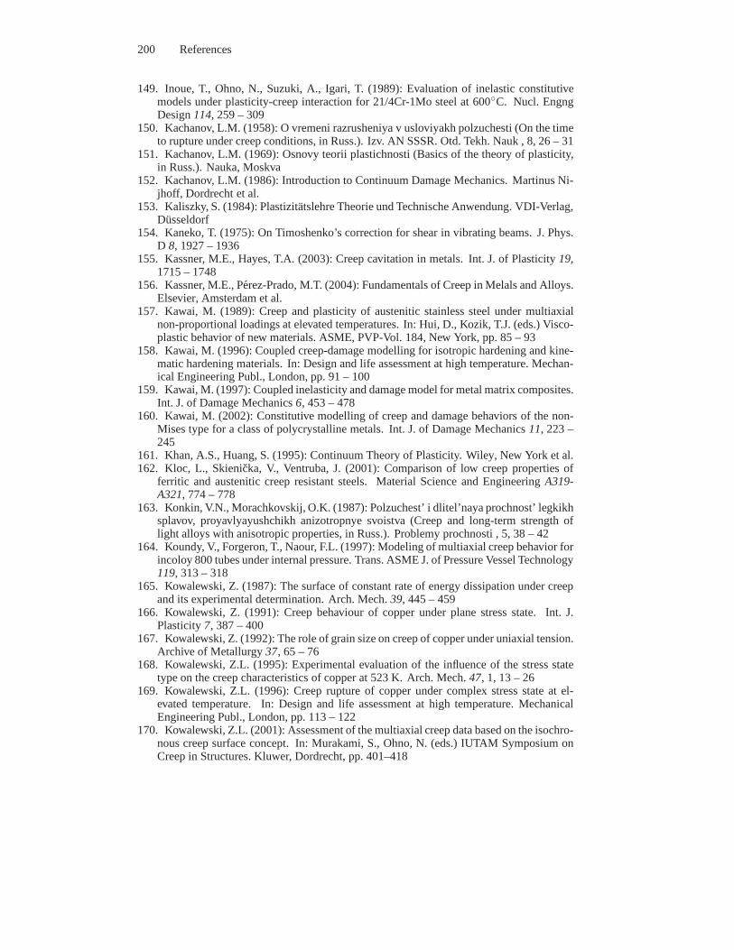
200 References
149. Inoue, T., Ohno, N., Suzuki, A., Igari, T. (1989): Evaluation of inelastic constitutivemodels under plasticity-creep interaction for 21/4Cr-1Mosteel at 600C. Nucl. EngngDesign114, 259 – 309
150. Kachanov, L.M. (1958): O vremeni razrusheniya v usloviyakh polzuchesti (On the timeto rupture under creep conditions, in Russ.). Izv. AN SSSR. Otd. Tekh. Nauk , 8, 26 – 31
151. Kachanov, L.M. (1969): Osnovy teorii plastichnosti (Basics of the theory of plasticity,in Russ.). Nauka, Moskva
152. Kachanov, L.M. (1986): Introduction to Continuum Damage Mechanics. Martinus Ni-jhoff, Dordrecht et al.
153. Kaliszky, S. (1984): Plastizitatslehre Theorie und Technische Anwendung. VDI-Verlag,Dusseldorf
154. Kaneko, T. (1975): On Timoshenko’s correction for shear in vibrating beams. J. Phys.D 8, 1927 – 1936
155. Kassner, M.E., Hayes, T.A. (2003): Creep cavitation inmetals. Int. J. of Plasticity19,1715 – 1748
156. Kassner, M.E., Perez-Prado, M.T. (2004): Fundamentals of Creep in Melals and Alloys.Elsevier, Amsterdam et al.
157. Kawai, M. (1989): Creep and plasticity of austenitic stainless steel under multiaxialnon-proportional loadings at elevated temperatures. In: Hui, D., Kozik, T.J. (eds.) Visco-plastic behavior of new materials. ASME, PVP-Vol. 184, New York, pp. 85 – 93
158. Kawai, M. (1996): Coupled creep-damage modelling for isotropic hardening and kine-matic hardening materials. In: Design and life assessment at high temperature. Mechan-ical Engineering Publ., London, pp. 91 – 100
159. Kawai, M. (1997): Coupled inelasticity and damage model for metal matrix composites.Int. J. of Damage Mechanics6, 453 – 478
160. Kawai, M. (2002): Constitutive modelling of creep and damage behaviors of the non-Mises type for a class of polycrystalline metals. Int. J. of Damage Mechanics11, 223 –245
161. Khan, A.S., Huang, S. (1995): Continuum Theory of Plasticity. Wiley, New York et al.162. Kloc, L., Skienicka, V., Ventruba, J. (2001): Comparison of low creep properties of
ferritic and austenitic creep resistant steels. Material Science and EngineeringA319-A321, 774 – 778
163. Konkin, V.N., Morachkovskij, O.K. (1987): Polzuchest’ i dlitel’naya prochnost’ legkikhsplavov, proyavlyayushchikh anizotropnye svoistva (Creep and long-term strength oflight alloys with anisotropic properties, in Russ.). Problemy prochnosti , 5, 38 – 42
164. Koundy, V., Forgeron, T., Naour, F.L. (1997): Modelingof multiaxial creep behavior forincoloy 800 tubes under internal pressure. Trans. ASME J. ofPressure Vessel Technology119, 313 – 318
165. Kowalewski, Z. (1987): The surface of constant rate of energy dissipation under creepand its experimental determination. Arch. Mech.39, 445 – 459
166. Kowalewski, Z. (1991): Creep behaviour of copper underplane stress state. Int. J.Plasticity7, 387 – 400
167. Kowalewski, Z. (1992): The role of grain size on creep ofcopper under uniaxial tension.Archive of Metallurgy37, 65 – 76
168. Kowalewski, Z.L. (1995): Experimental evaluation of the influence of the stress statetype on the creep characteristics of copper at 523 K. Arch. Mech.47, 1, 13 – 26
169. Kowalewski, Z.L. (1996): Creep rupture of copper undercomplex stress state at el-evated temperature. In: Design and life assessment at high temperature. MechanicalEngineering Publ., London, pp. 113 – 122
170. Kowalewski, Z.L. (2001): Assessment of the multiaxialcreep data based on the isochro-nous creep surface concept. In: Murakami, S., Ohno, N. (eds.) IUTAM Symposium onCreep in Structures. Kluwer, Dordrecht, pp. 401–418
References 201
171. Kowalewski, Z.L., Hayhurst, D.R., Dyson, B.F. (1994):Mechanisms-based creep con-stitutive equations for an aluminium alloy. J. Strain Anal.29, 4, 309 – 316
172. Krajcinovic, D. (1996): Damage Mechanics. Applied Mathematics and Mechanics Vol.41. North-Holland, Amsterdam et al.
173. Kraus, H. (1980): Creep Analysis. John Wiley & Sons, NewYork et al.174. Krausz, A.S., Krausz, K. (1996): Unified constitutive laws of plastic deformation. Aca-
demic press, San Diego et al.175. Krawietz, A. (1986): Materialtheorie. MathematischeBeschreibung des phanomenolo-
gischen thermomechanischen Verhalten. Springer, Berlin et al.176. Krempl, E. (1999): Creep-plasticity interaction. In:Altenbach, H., Skrzypek, J. (eds.)
Creep and Damage in Materials and Structures. Springer, Wien, New York, pp. 285 –348. CISM Lecture Notes No. 399
177. Krieg, R. (1999): Reactor Pressure Vessel Under SevereAccident Loading. Final Reportof EU-Project Contract FI4S-CT95-0002. Technical report,Forschungszentrum Karl-sruhe, Karlsruhe
178. Lai, W.M., Rubin, D., Krempl, E. (1993): Introduction to Continuum Mechanics. Perg-amon Press, Oxford et al.
179. Lazan, B.J. (1949): Dynamic creep and rupture properties of temperature-resistant ma-terials under tensile fatigue stress. Proc. ASTM49, 757 – 787
180. Le May, I., da Silveria, T.L., Cheung-Mak, S.K.P. (1994): Uncertainties in the evalua-tions of high temperature damage in power stations and petrochemical plant. Int. J. ofPressure Vessels & Piping59, 335 – 343
181. Leal, L.G., Hinch, E.J. (1973): Theoretical studies ofa suspension of rigid particlesaffected by Brownian couples. Rheol. Acta12, 127–132
182. Leckie, F.A., Hayhurst, D.R. (1977): Constitutive equations for creep rupture. ActaMetall. 25, 1059 – 1070
183. Lemaitre, J. (1996): A Course on Damage Mechanics. Springer, Berlin et al.184. Lemaitre, J. (ed.) (2001): Handbook of Materials Behavior Models. Academic Press,
San Diego185. Lemaitre, J., Chaboche, J.L. (1990): Mechanics of Solid Materials. Cambridge Univer-
sity Press, Cambridge186. Levinson, M. (1981): A new rectangular beam theory. J. Sound Vibr.74, 81 – 87187. Lewin, G., Lehmann, B. (1977): Ergebnisse uber das Spannungs-Verformungsverhalten
von PVC, dargestellt an einem zylindrischen Bauelement. Wiss. Z. TH Magdeburg21,415 – 422
188. Libai, A., Simmonds, J.G. (1998): The nonlinear theoryof elastic shells. CambridgeUniversity Press, Cambridge
189. Lin, J., Dunne, F.P.E., Hayhurst, D.R. (1999): Aspectsof testpiece design responsiblefor errors in cyclic plasticity experiments. Int. J. of Damage Mechanics8, 109 – 137
190. Lin, T.H. (1962): Bending of a plate with nonlinear strain hardening creep. In: Hoff,N.J. (ed.) Creep in Structures. Springer, Berlin et al., pp.215 – 228
191. Lippmann, H. (1993): Angewandte Tensorrechnung. Springer, Berlin et al.192. Liu, Y., Murakami, S. (1998): Damage localization of conventional creep damage mod-
els and proposition of a new model for creep damage analysis.JSME Int. J. Series A41,57 – 65
193. Liu, Y., Murakami, S., Kageyama, Y. (1994): Mesh-dependence and stress singularity infinite element analysis of creep crack growth by continuum damage mechanics approach.Eur. J. Mech. A/Solids35, 3, 147 – 158
194. Lo, K.H., Christensen, R.M., Wu, E.M. (1977): A high–order theory of plate deforma-tion. Part I: Homogeneous Plates. Transactions of the American Society of MechanicalEngineers. Journal of Applied Mechanics44, 4, 663–668
195. Lucas, G.E., Pelloux, R.M.N. (1981): Texture and stress state dependent creep inZircaloy-2. Metallurgical Transactions A12A, 1321 – 1331
202 References
196. Ludeke, M., Schmidt, R. (1992): Current design practice for high temperature compo-nents in fossil power plants and chemical plants in Germany.In: Larson, L.H. (ed.) HighTemperature Structural Design. Mechanical Engineering Publications, London, pp. 3 –20
197. Lundin, C.D., Liu, P., Prager, M. (2001): Creep behavior of weld heat affected zoneregions for modified 9Cr-1Mo Steel. In: Proceedings of CREEP7. Japan Society of Me-chanical Engineers, Tsukuba, pp. 379 – 436
198. Lurie, A.I. (1970): Lineinaya teoriya uprugosti (Linear Theory of Elasticity, in Russ.).Nauka, Moskva
199. Lurie, A.I. (1990): Nonlinear Theory of Elasticity. North-Holland, Dordrecht200. Mahnken, R. (1998): Anisotropic creep modeling based on elastic projection operators
with applications to CMSX-4 superalloy. Int. J. Mech. Sci.14, 235 – 280201. Malinin, N.N. (1975): Prikladnaya teoriya plastichnosti i polzuchesti (Applied theory
of plasticity and creep, in Russ.). Mashinostroenie, Moskva202. Malinin, N.N. (1981): Raschet na polzuchest’ konstrukcionnykh elementov (Creep cal-
culations of structural elements, in Russ.). Mashinostroenie, Moskva203. Malinin, N.N., Khadjinsky, G.M. (1969): K postroeniyuteorii polzuchesti s anizotrop-
nym uprochneniem (On the formulation of a creep theory with anisotropic hardening, inRuss.). Izv. AN SSSR. Mechanika tverdogo tela3, 148 – 152
204. Malinin, N.N., Khadjinsky, G.M. (1972): Theory of creep with anisotropic hardening.Int. J. Mech. Sci.14, 235 – 246
205. Matsui, M., Tabuchi, M., Watanabe, T., Kubo, K., Kinugawa, J., Abe, F. (2001): Degra-dation of creep strength in welded joint of 9%Cr steel. ISIJ International41, S126 –S130
206. Maugin, G.A. (1992): The Thermomechanics of Plasticity and Fracture. CambridgeUniversity Press, Cambridge
207. Meenen, J., Altenbach, H. (2001): A consistent deduction of von Karman-type platetheories from threedimensional non-linear continuum mechanics. Acta Mechanica147,1 – 17
208. Miller, A.K. (ed.) (1987): Unified constitutive equations for creep and plasticity. Else-vier, London, New York
209. Miyazaki, N. (1987): Creep buckling analyses of circular cylindrical shells under axialcompression-bifurcation buckling analysis by the finite element method. Trans. ASME.J. Pressure Vessel Technol.109, 179 – 183
210. Miyazaki, N. (1988): Creep buckling analyses of circular cylindrical shell under bothaxial compression and internal or external pressure. Computers & Structures28, 437 –441
211. Mohrmann, R., Sester, M. (1999): A multiaxial model forthe evolution of the mi-crostructure and for the mechanical behaviour of a 12% chromium steel under creepconditions. In: Mugharbi, H., Gottstein, G., Mecking, H., Riedel, H., Tobolski, J. (eds.)Microstructure and Mechanical Properties of Metallic High-Temperature Materials: Re-search Report/DFG. Wiley-VCH, Weinheim, pp. 206 – 221
212. Morishita, T., Hirao, M. (1997): Creep damage modelling based on ultrasonic velocitiesin copper. Int. J. Solids and Structures34, 1169 – 1182
213. Mucke, R., Bernhardi, O. (2003): A constitutive modelfor anisotropic materials basedon Neuber’s rule. Comput. Methods Appl. Mech. Engrg.192, 4237 – 4255
214. Muhlhaus, H.B. (ed.) (1995): Continuum Models for Materials with Microstructure.John Wiley & Sons, Chichester et al.
215. Murakami, S. (1983): Notion of continuum damage mechanics and its application toanisotropic creep damage theory. ASME J. Engng. Mat. Tech.105, 99 – 105
216. Murakami, S., Liu, Y. (1995): Mesh-dependence in localapproach to creep fracture.Int. J. of Damage Mech.4, 230 – 250
References 203
217. Murakami, S., Ohno, N. (1981): A continuum theory of creep and creep damage. In:Ponter, A.R.S., Hayhurst, D.R. (eds.) Creep in Structures.Springer, Berlin, pp. 422 – 444
218. Murakami, S., Sanomura, Y. (1985): Creep and creep damage of copper under multi-axial states of stress. In: Sawczuk, A., Bianchi, B. (eds.) Plasticity Today – Modelling,Methods and Applications. Elsevier, London, New York, pp. 535 – 551
219. Murakami, S., Sanomura, Y., Hattori, M. (1986): Modelling of the coupled effect ofplastic damage and creep damage in Nimonic 80A. Int. J. Solids and Structures22, 4,373 – 386
220. Murakami, S., Suzuki, K. (1971): On the creep analysis of pressurized circular cylin-drical shells. Int. J. Non-Linear Mechanics6, 377 – 392
221. Murakami, S., Suzuki, K. (1973): Application of the extended Newton method to thecreep analysis of shells of revolution. Ing.-Arch.42, 194 – 207
222. Nabarro, F.R.N., de Villiers, H.L. (1995): The Physicsof Creep. Creep and Creep-resistant Alloys. Taylor & Francis, London
223. Naghdi, P.M. (1990): A critical review of the state of finite plasticity. J. of App. Math.and Phys. (ZAMP)41, 316 – 394
224. Naumenko, K. (1996): Modellierung und Berechnung der Langzeitfestigkeitdunnwandiger Flachentragwerke unter Berucksichtigung von Werkstoffkriechen undSchadigung. Dissertation, Otto-von-Guericke-Universitat Magdeburg
225. Naumenko, K. (2000): On the use of the first order shear deformation models of beams,plates and shells in creep lifetime estimations. Technische Mechanik20, 3, 215 – 226
226. Naumenko, K., Altenbach, H. (2005): A phenomenological model for anisotropic creepin a multi-pass weld metal. Arch. Appl. Mech.75, 808–819
227. Naumenko, K., Altenbach, J., Altenbach, H., Naumenko,V.K. (2001): Closed and ap-proximate analytical solutions for rectangular Mindlin plates. Acta Mechanica147, 153–172
228. Nikitenko, A.F. (1984): Eksperimental’noe obosnovanie gipotezy suschestvovaniyapoverkhnosti polzuchesti v usloviyakh slozhnogo nagruzheniya, (Experimental justifica-tion of the hypothsis on existence of the creep surface undercomplex loading conditions,in Russ.). Problemy prochnosti , 8, 3 – 8
229. Niu, L., Kobayashi, M., Takaku, H. (2002): Creep rupture properties of an austeniticsteel with high ductility under multi-axial stresses. ISIJInternational42, 1156 – 1181
230. Noll, W. (1972): A new mathematical theory of simple materials. Arch. Rat. Mech.Anal. 48, 1 – 50
231. Nowacki, W. (1986): Theory of Asymmetric Elasticity. Pergamon Press, Oxford et al.232. Nye, J.F. (1992): Physical Properties of Crystals. Oxford Science Publications, Oxford233. Odqvist, F.K.G. (1962): Applicability of the elastic analogue to creep problems of
plates, membranes and beams. In: Hoff, N.J. (ed.) Creep in Structures. Springer, Berlinet al., pp. 137 – 160
234. Odqvist, F.K.G. (1974): Mathematical Theory of Creep and Creep Rupture. OxfordUniversity Press, Oxford et al.
235. Odqvist, F.K.G. (1981): Historical survay of the development of creep mechanics fromits beginnings in the last century to 1970. In: Ponter, A.R.S., Hayhurst, D.R. (eds.) Creepin Structures. Springer, Berlin et al., pp. 1 – 12
236. Odqvist, F.K.G., Hult, J. (1962): Kriechfestigkeit metallischer Werkstoffe. Springer,Berlin u.a.
237. Ohno, N. (1990): Recent topics in constitutive modelling of cyclic plasticity and vis-coplasticity. Appl. Mech. Rev.43, 283 – 295
238. Ohno, N., Kawabata, M., Naganuma, J. (1990): Aging effects on monotonic, stress-paused, and alternating creep of type 304 stainless steel. Int. J. of Plasticity6, 315 –327
204 References
239. Ohno, N., Takeuchi, T. (1994): Anisotropy in multiaxial creep of nickel-based single-crystal superalloy CMSX-2 (experiments and identificationof active slip systems). JSMEInt. J. Series A37, 129 – 137
240. Onat, E.T., Leckie, F.A. (1988): Representation of mechanical behavior in the presenceof changing internal structure. Trans. ASME J. Appl. Mech.55, 1 – 10
241. Onck, P.R., Nguyen, B.N., der Giessen, E.V. (2000): Microstructural modelling of creepfracture in polycrystalline materials. In: Murakami, S., Ohno, N. (eds.) Creep in Struc-tures. Kluwer Academic Publishers, Dordrecht et al., pp. 51– 64
242. Orlova, A., Bursık, J., Kucharova, K., Sklenicka, V. (1998): Microstructural develop-ment during high temperature creep of 9% Cr steel. Material Science and EngineeringA245, 39 – 48
243. Othman, A.M., Dyson, B.F., Hayhurst, D.R., Lin, J. (1994): Continuum damage me-chanics modelling of circumferentially notched tension bars undergoing tertiary creepwith physically-based constitutive equations. Acta Metall. Mater.42, 3, 597 – 611
244. Othman, A.M., Hayhurst, D.R., Dyson, B.F. (1993): Skeletal point stresses in circum-ferentially notched tension bars undergoing tertiary creep modelled with physically-based constitutive equations. Proc. R. Soc. Lond.A441, 343 – 358
245. Oytana, C., Delobelle, P., Mermet, A. (1982): Constitutive equations study in biaxialstress experimants. Trans. ASME J. of Engineering Materials and Technology104, 3, 1– 11
246. Palmov, V. (1998): Vibrations in Elasto-Plastic Bodies. Springer, Berlin et al.247. Peirce, D., Shih, C.F., Needleman, A. (1984): A tangentmodulus method for rate de-
pendent solids. Comp. & Structures18, 875 – 887248. Penkalla, H.J., Schubert, F., Nickel, H. (1988): Torsional creep of alloy 617 tubes at
elevated temperature. In: Reichman, S., Duhl, D.N., Maurer, G., Antolovich, S., Lund,C. (eds.) Superalloys 1988. The Metallurgical Society, pp.643 – 652
249. Penny, R.K. (1964): Axisymmetrical bending of the general shell of revolution duringcreep. J. Mech. Eng. Sci.6, 44 – 45
250. Penny, R.K., Mariott, D.L. (1995): Design for Creep. Chapman & Hall, London et al.251. Perrin, I.J., Hayhurst, D.R. (1994): Creep constitutive equations for a 0.5Cr-0.5Mo-
0.25V ferritic steel in the temperature range 600-675C. J. Strain Anal.31, 4, 299 –314
252. Perrin, I.J., Hayhurst, D.R. (1999): Continuum damagemechanics analyses of type IVcreep failure in ferritic steel crossweld specimens. Int. J. Pressure Vessels Piping76, 599– 617
253. Pilkey, W.D., Wunderlich, W. (1994): Mechanics of Structures: Variational and Com-putational Methods. CRC Press, Boca Raton et al.
254. Pintschovius, L., Gering, E., Munz, D., Fett, T., Soubeyroux, J.L. (1989): Determina-tion of non-symmetric secondary creep behaviour of ceramics by residual stress mea-surements using neutron diffractometry. J. Mater. Sci. Lett. 8, 7, 811 – 813
255. Podgorny, A.N., Bortovoj, V.V., Gontarovsky, P.P., Kolomak, V.D., Lvov, G.I.,Matyukhin, Y.J., Morachkovsky, O.K. (1984): Polzuchest’ elementov mashinostroi-tel’nykh konstrykcij (Creep of mashinery structural members, in Russ.). Naukova dumka,Kiev
256. Powell, P.C. (1994): Engineering with fiber-reinforced laminates. Chapman & Hall,London et al.
257. Prager, W. (1956): A new method of analyzing stresses and strains in work-hardeningplastic solids. J. Appl. Mech.23, 4, 493 – 496
258. ANSYS, Inc. Theory Manual (2001): Swanson Analysis Systems, Inc.259. Qi, W. (1998): Modellierung der Kriechschadigung einkristalliner Superlegierungen
im Hochtemperaturbereich, Fortschrittberichte VDI, Reihe 18, Nr. 230. VDI Verlag,Dusseldorf
References 205
260. Qi, W., Bertram, A. (1997): Anisotropic creep damage modelling of single crystal su-peralloys. Technische Mechanik17, 4, 313 – 322
261. Qi, W., Bertram, A. (1998): Damage modeling of the single crystal superalloy SRR99under monotonous creep. Comp. Mater. Sci.13, 132 – 141
262. Qi, W., Bertram, A. (1999): Anisotropic continuum damage modeling for single crystalsat high temperatures. Int. J. Plasticity15, 1197 – 1215
263. Rabotnov, Y.N. (1959): O mechanizme dlitel’nogo razrusheniya (A mechanism of thelong term fracture, in Russ.). Voprosy prochnosti materialov i konstruktsii, AN SSSR , 5– 7
264. Rabotnov, Y.N. (1963): O razrushenii vsledstvie polzuchesti (On fracture as a conse-quence of creep, in Russ.). Prikladnaya mekhanika i tekhnicheskaya fizika2, 113 – 123
265. Rabotnov, Y.N. (1969): Creep Problems in Structural Members. North-Holland, Ams-terdam
266. Rabotnov, Y.N. (1979): Mekhanika deformiruemogo tverdogo tela (Mechanics of thedeformable solid, in Russ.). Nauka, Moskva
267. Reddy, J.N. (1984): A simple higher-order theory for laminated composite plate. Trans.ASME. J. Appl. Mech.51, 745 – 752
268. Reddy, J.N. (1997): Mechanics of Laminated Composite Plates: Theory and Analysis.CRC Press, Boca Raton et al.
269. Reiner, M. (1969): Deformation and Flow. An ElementaryIntroduction to Rheology.3rd edition. H.K. Lewis & Co., London
270. Reissner, E. (1950): A variational theorem in elasticity. J. Math. Phys.29, 90 – 95271. Riedel, H. (1987): Fracture at High Temperatures. Materials Research and Engineering.
Springer, Berlin et al.272. Robinson, D.N. (1984): Constitutive relationships for anisotropic high-temperature al-
loys. Nuclear Engineering Design83, 389 – 396273. Robinson, D.N., Binienda, W.K., Ruggles, M.B. (2003):Creep of polymer matrix com-
posites. I: Norton/Bailey Creep Law for transverse isotropy. J. of Engineering Mechanics,ASCE129, 3, 310 – 317
274. Robinson, D.N., Binienda, W.K., Ruggles, M.B. (2003):Creep of polymer matrix com-posites. II: Monkman-Grant failure relationship for transverse isotropy. J. of EngineeringMechanics, ASCE129, 3, 318 – 323
275. Roche, R.L., Townley, C.H.A., Regis, V., Hubel, H. (1992): Structural analysis andavailable knowledge. In: Larson, L.H. (ed.) High Temperature Structural Design. Me-chanical Engineering Publications, London, pp. 161 – 180
276. Rodin, G.J. (2000): Continuum damage mechanics and creep analysis. J. of Appl.Mech. ASME67, 193 – 196
277. Rodin, G.J., Parks, D.M. (1986): Constitutive models of a power-law matrix containingaligned penny-shaped cracks. Mechanics of Materials5, 221 – 228
278. Rodin, G.J., Parks, D.M. (1988): A self-consistent analysis of a creeping matrix withaligned cracks. J. Mech. Phys. Solids36, 237 – 249
279. Rogers, T.G. (1990): Yield criteria, flow rules and hardening in anisotropic plasticity.In: Boehler, J.P. (ed.) Yielding, Damage and Failure of Anisotropic Solids. MechanicalEngineering Publications, London, pp. 53 – 79
280. Rychlewski, J., Zhang, J. (1991): On representation oftensor functions: a rerview. Ad-vances in Mechanics14, 75 – 94
281. Saanouni, K., Chaboche, J.L., Lense, P.M. (1989): On the creep crack-growth predictionby a non-local damage formulation. Eur. J. Mech. A/Solids8, 6, 437 – 459
282. Sakane, M., Hosokawa, T. (2001): Biaxial and triaxial creep testing of type 304 stainlesssteel at 923 K. In: Murakami, S., Ohno, N. (eds.) IUTAM Symposium on Creep inStructures. Kluwer, Dordrecht, pp. 411–418
283. Sakane, M., Tokura, H. (2002): Experimental study of biaxial creep damage for type304 stainless steel. Int. J. of Damage Mechanics11, 247 – 262
206 References
284. Schiesse, P. (1994): Ein Beitrag zur Berechnung des Deformationsverhaltens anisotropgescheadigter Kontinua unter Berucksichtigung der thermoplastischer Kopplung. Disser-tation, Ruhr-Universitat Bochum, Mitteilungen aus dem Institut fur Mechanik 89
285. Schroder, J., Gross, D. (2004): Invariant formulation of the electromechanical enthalpyfunction of transversely isotropic piezoelectric materials. Arch. Appl. Mech73, 533 –552
286. Schroder, J., Neff, P. (2003): Invariant formulationof hyperelastic transverse isotropybased on polyconvex free energy functions. Int. J. Solids and Structures40, 401 – 445
287. Schwetlick, H., Kretzschmar, H. (1991): Numerische Verfahren fur Naturwis-senschaftler und Ingenieure. Fachbuchverlag, Leipzig
288. Sdobyrev, V.P. (1959): Kriterij dlitel’noj prochnosti dlya nekotorykh zharoprochnykhsplavov pri slozhnom napryazhennom sostoyanii, (Criterion of long term strength ofsome high-temperature alloys under multiaxial stress state, in Russ.). Izv. AN SSSR.OTN. Mekh. i Mashinostroenie , 6, 93 – 99
289. Segle, P., Tu, S.T., Storesund, J., Samuelson, L.A. (1996): Some issues in life assess-ment of longitudinal seam welds based on creep tests with cross-weld specimens. Int. J.of Pressure Vessels & Piping66, 199 – 222
290. Shibli, I.A. (2002): Performance of P91 thick section welds under steady and cyclicloading conditions: power plant and research experience. OMMI 1, 3. Available fromhttp://www.ommi.co.uk
291. Skrzypek, J., Ganczarski, A. (1998): Modelling of Material Damage and Failure ofStructures. Foundation of Engineering Mechanics. Springer, Berlin et al.
292. Skrzypek, J.J. (1993): Plasticity and Creep. CRC Press, Boca Raton et al.293. Smith, D.R. (1993): An Introduction to Continuum Mechanics. Kluwer, Dordrecht et
al.294. Solocevskij, A., Konkin, V., Morackowskij, O., Koczyk, S. (1985): Eine Theorie zur
nichtlinearen Verformung anisotroper Korper und ihre Anwendung auf die Berechnungdes Kriechverhaltens dunner Schalen. Technische Mechanik 6, 4, 27 – 36
295. Sosnin, O.V. (1971): K voprosu o suschestvovanii potentsiala polzuchseti, (On the ques-tion on existense of creep potential, in Russ.). Izv. AN SSSRMekhanika tverdogo tela ,5, 85 – 89
296. Sosnin, O.V. (1974): Energeticheskii variant teorii polzuchesti i dlitel’noi prochnosti.Polzuchest’ i razrushenie neuprochnyayushikhsya materialov (Energetic variant of thecreep and long–term strength theories. Creep and fracture of nonhardening materials, inRuss.). Problemy prochnosti , 5, 45 – 49
297. Sosnin, O.V., Gorev, B.V., Nikitenko, A.F. (1986): Energeticheskii variant teoriipolzuchesti (Energetic variant of the creep theory, in Russ.). Institut Gidrodinamiki,Novosibirsk
298. Spencer, A.J.M. (1984): Linear elastic constitutive equations for fibre-reinforced mate-rial. In: Spencer, A.J.M. (ed.) Continuum Theory of the Mechanics of Fibre-ReinforcedComposites. Springer-Verlag, Wien et al., pp. 1–32
299. Spencer, A.J.M. (1987): Isotropic polynomial invariants and tensor functions. In:Boehler, J.P. (ed.) Applications of tensor functions in solid mechanics. Springer, Wienet al., pp. 141–169
300. Stamm, H., von Estroff, U. (1993): Determination of damage parameters for microck-rack formation under creep conditions. In: Ainsworth, R.A., Skelton, R.P. (eds.) Behav-iour of Defects at High Temperatures. Mechanical Engineering Publications, London, pp.123 – 151
301. Stouffer, D.C., Dame, L.T. (1996): Inelastic deformation of metals. John Wiley & Sons,New York
302. Taira, S. (1962): Lifetime of structures subjected to varying load and temperature. In:Hoff, N.J. (ed.) Creep in Structures. Springer, Berlin et al., pp. 96 – 119
References 207
303. Taira, S., Koterazawa, R. (1962): Dynamic creep and fatigue of an 18-8-Mo-Nb Steel.Bull. JSME5, 17, 15 – 20
304. Taira, S., Ohtani, R. (1986): Teorija vysokotemperaturnoj prochnosti materialov (The-ory of high-temperature strength of materials, in Russ.). Metallurgija, Moscow
305. Takezono, S., Fujoka, S. (1981): The creep of moderately thick shells of revolutionunder axisymmetrical load. In: Ponter, A.R.S., Hayhurst, D.R. (eds.) Creep in Structures.Springer-Verlag, Berlin et al., pp. 128 – 143
306. Takezono, S., Migita, K., Hirakawa, A. (1988): Elastic/Visco-plastic deformation ofmulti-layered shells of revolution. JSME, Ser. 131, 3, 536 – 544
307. Tamuzh, V.P., Kuksenko, V.S. (1978): Mikromeckanika razrusheniya polimernykh ma-terialov (Micromechanics of fracture of polymeric materials, in Russ.). Zinatne, Riga
308. Timoshenko, S.P. (1953): History of Strength of Materials. Dover Publications, NewYork
309. Ting, T.C.T. (1996): Anisotropic Elasticity. Theory and Applications. Oxford Univer-sity Press, Oxford et al.
310. Trivaudey, F., Delobelle, P. (1993): Experimental study and modelization of creep dam-age under multi-axial loadings at high temperature. In: Wilshire, B., Evans, R.W. (eds.)Creep and Fracture of Engineering Materials and Structures. Institute of Materials, Lon-don, pp. 137–147
311. Trostel, R. (1993): Mathematische Grundlagen der Technischen Mechanik I Vektor-und Tensoralgebra. Vieweg, Braunschweig et al.
312. Truesdell, C. (1964): Second-Order Effects in the Mechanics of Materials. In: Reiner,M., Abir, D. (eds.) Second-Order Effects in Elasticity, Plasticity and Fluid Dynamics.Pergamon Press, Oxford et al., pp. 228 – 251
313. Truesdell, C., Noll, W. (1992): The Non-Linear Field Theories of Mechanics. 2ndedition. Springer, Berlin et al.
314. Trunin, I.I. (1965): Kriterii prochnosti v usloviyakhpolzuchesti pri slozhnomnapryazhennom sostoyanii (Failure criteria under creep conditions in multiaxial stressstate, in Russ. Prikl. Mekhanika1, 7, 77 – 83
315. Tvergaard, V. (1990): Material failure by void growth to coalescence. Advances inApplied Mechanics27, 83 – 51
316. Vakulenko, A.A., Kachanov, M.L. (1971): Kontinual’naya teoria sredy s teshchinami(Continuum theory of a medium with cracks, in Russ.). Izv. ANSSSR. Mekhanika tver-dogo tela , 4, 159 – 166
317. van der Giessen, E., Tvergaard, V. (1995): Developmentof final creep failure in poly-crystalline aggregates. Acta Metall. Mater.42, 959 – 973
318. van der Giessen, E., van der Burg, M.W.D., Needleman, A., Tvergaard, V. (1995): Voidgrowth due to creep and grain boundary diffusion at high triaxialities. J. Mech. Phys.Solids43, 123 – 165
319. von Karman, T. (1911): Festigkeitsprobleme im Maschinenbau. In: Encyklop. d. math.Wissensch. IV/2. Teubner, Leipzig, pp. 311 – 385
320. von Mises, R. (1928): Mechanik der plastischen Formanderung von Kristallen. ZAMM8, 3, 161 – 185
321. Washizu, K. (1982): Variational Methods in Elasticityand Plasticity. Pergamon Press,Oxford et al.
322. Weber, J., Klenk, A., Rieke, M. (2005): A new method of strength calculation andlifetime prediction of pipe bends operating in the creep range. Int. J. of Pressure Vesselsand Piping82, 77 – 84
323. Winstone, M.R. (1998): Microstructure and alloy developments in nickel-based super-alloys. In: Strang, A., Cawley, J., Greenwood, G.W. (eds.) Microstructural Stability ofCreep Resistant Alloys for High Temperature Plant Applications. Cambridge UniversityPress, Cambridge, pp. 27 – 47
208 References
324. Wohlfahrt, H., Brinkmann, D. (2001): Consideration ofinhomogeneties in applicationof deformation models, describing the inelastic behaviourof welded joints. In: Steck,E., Ritter, R., Peil, U., Ziegenbein, A. (eds.) Plasticity of Metals: Experiments, Models,Computation. Final Report of the Collaborative Research Centre 319, Stoffgesetze furdas inelastische Verhalten metalischer Werkstoffe - Entwicklung und technische Anwen-dung. Wiley-VCH, Weinheim, pp. 361 – 382
325. Wriggers, P. (2001): Nichtlineare Finite-Element-Methoden. Springer, Berlin et al.326. Wu, R., Sandstrom, R., Seitisleam, F. (2004): Influence of extra coarse grains on the
creep properties of 9 percent CrMoV (P91) steel weldment. Trans. ASME Journal ofEngineering Materials and Technology26, 87 – 94
327. Wu, Z. (1993): Kriechen und Kriechschadigung von Eis unter mehrachsiger Belastung,Fortschrittberichte VDI, Reihe 18, Nr. 135. VDI Verlag, Dusseldorf
328. Xiao, H., Bruhns, O., Meyers, A. (2000): Minimal generating sets for symmetric 2nd-order tensor-valued transversely isotropic functions of vectors and 2nd-order tensors.ZAMM 80, 565 – 569
329. Yang, H.T.Y., Saigal, S., Masud, A., Kapania, R.K. (2000): A survey of recent shellfinite elements. Int. J. Numer. Meth. Engng.47, 101 – 127
330. Zheng, Q.S. (1994): Theory of representations of tensor functions. Appl. Mech. Rev.47, 11, 545 – 587
331. Zheng, Q.S., Boehler, J.P. (1994): The description, classification and reality of materialand physical symmetries. Acta Mechanica102, 73 – 89
332. Zhilin, P.A. (1982): Osnovnye uravneniya neklassicheskoi teorii obolochek (Basicequations of a non-classical theory of shells, in Russ.). Dinamika i prochnost’ mashin,Trudy LPI 386, 29 – 46
333. Zhilin, P.A. (1996): A new approach to the analysis of free rotations of rigid bodies.ZAMM 4, 187 – 204
334. Zhilin, P.A. (2001): Vektory i tensory vtorogo ranga v trekhmernom prostranstve (Vec-tors and second rank tensors in three-dimensional space, inRuss.). Nestor, St. Petersburg
335. Zhilin, P.A. (2003): Modifizirovannaya teoriya simmetrii tenzorov i tenzornykh in-variantov (A modified theory of symmetry for tensors and tensor invariants, in Russ.).Izvestiya vuzov. Estestvennye Nauki , 176 – 195
336. Zhilin, P.A., Ivanova, E.A. (1995): Modifitsirovannyifunktsional energii v teorii plastintipa Reissnera (A modified energy functional in the Reissnertype plate theory, in Russ.).Mekhanika tverdogo tela2, 120 – 128
337. Ziegler, H. (1963): Some extremum principles in irreversible thermodynamics with ap-plication to continuum mechanics. In: Sneddon, I.N., Hill,R. (eds.) Progress in SolidMechanics. North-Holland, Amsterdam, pp. 93 – 192
338. Zienkiewicz, O.C., Taylor, R.L. (1991): The Finite Element Method. McGraw-Hill,London et al.
339. Zolochevskij, A.A. (1988): Kriechen von Konstruktionselementen aus Materialien mitvon der Belastung abhangigen Charakteristiken. Technische Mechanik9, 177 – 184
340. Zurmuhl, R., Falk, S. (1992): Matrizen und ihre Anwendungen. Springer, Berlin et al.341. Zyczkowski, M. (2000): Creep damage evolution equations expressed in terms of dis-
sipated power. Int. J. Mech. Sci.42, 755 – 769

Eidesstattliche Erkl arung
Hiermit erklare ich eidesstattlich, dass ich die vorgelegte Habilitationsschriftselbstandig und nur unter Verwendung der angegebenen Literatur und Hilfsmittelangefertigt habe.
Halle, 11.04.2006 Konstantin Naumenko
Lebenslauf
Persönliche Daten
Konstantin NaumenkoKröllwitzer Str. 2006120 Halle
Tel.: (03 45) 550 70 36
geb. am 03. 08. 1966 in Kharkov, Ukraine
seit 1991 verheiratet mit Viktoria Naumenko (geb. Gromova)Sohn Daniel (geb. 1996)Tochter Anna (geb. 2003)
09/1973 – 05/1983 Schulbesuch in Kharkov, Ukraine
09/1983 – 02/1989 Studium an der Polytechnischen UniversitätKharkov (Ukraine), Fachrichtung Dynamik und Festigkeitvon Maschinen
02/1988 – 05/1988 Studienaufenthalt an der Otto-von-Guericke-Universität Mag-deburg
02/1989 Diplomarbeit an der Polytechnischen Universität Kharkov(Ukraine)
03/1989 – 01/1993 wissenschaftlicher Assistent am Lehrstuhl für Dynamik undFestigkeit von Maschinen der PU Kharkov (Ukraine)
02/1993 – 03/1996 Doktorand im Graduiertenkolleg „Modellierung, Berechnungund Identifikation mechanischer Systeme“ an der Otto-von-Guericke-Universität Magdeburg
seit 04/1996 wissenschaftlicher Mitarbeiter an der Martin-Luther-UniversitätHalle-Wittenberg am Institut für Prozess- und Stoffmodellie-rung, Lehrstuhl für Technische Mechanik
Halle, 11. April 2006