Embed Size (px)
Citation preview
Modeling of fiberglass reinforced epoxy composites
in LS-DYNA
Master Thesis
LIU-IEI-TEK-A--14/02048—SE
Marcus Menchawi Ludvig Almgren
Abstract
In this work, the modeling of glass fiber reinforced polymers (GFRP) in an FE-environment is in
focus. Two materials are investigated; both with a weave of perpendicular glass fibers that are soaked
in an epoxy matrix. In a military vehicle the survivability against threats such as explosive loads and
ballistic impacts is of great importance. At the same time there is an increasing demand for reduced
weight in the structure which makes GFRP an interesting alternative.
In order to analyze how the GFRP material will respond to an impact a material model must be
utilized and the input parameters established. The method will be used for analyses in the software LS-
DYNA. The material parameters was sought primarily by testing, however in order to make the
method complete literature studies have been made and also reversed engineering has been used. If an
appropriate material model can be combined with accurate material data realistic results can be
achieved and great resources can be saved that otherwise would have been used on impact testing.

Preface This master thesis is the final part of our Master of Science degree education in Mechanical
Engineering with focus on Applied Mechanics at Linköping University. The work has been done
during the spring of 2014 (January – June) at both Linköping University and at BAE Systems
Hägglunds in Örnsköldsvik. Our supervisor at BAE Systems has been Björn Zakrisson and our
supervisor at Linköping University has been Daniel Leidermark. The examiner has been Professor
Kjell Simonsson who also is located at Linköping University.
2014-06-23 Linköping

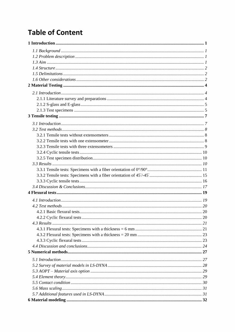
Table of Content 1 Introduction ........................................................................................................................................ 1
1.1 Background ................................................................................................................................... 1
1.2 Problem description ...................................................................................................................... 1
1.3 Aim ................................................................................................................................................ 1
1.4 Structure ........................................................................................................................................ 2
1.5 Delimitations ................................................................................................................................. 2
1.6 Other considerations ..................................................................................................................... 2
2 Material Testing ................................................................................................................................. 4
2.1 Introduction ................................................................................................................................... 4
2.1.1 Literature survey and preparations ......................................................................................... 4
2.1.2 S-glass and E-glass ................................................................................................................. 5
2.1.3 Test specimens ....................................................................................................................... 5
3 Tensile testing ..................................................................................................................................... 7
3.1 Introduction ................................................................................................................................... 7
3.2 Test methods .................................................................................................................................. 8
3.2.1 Tensile tests without extensometers ....................................................................................... 8
3.2.2 Tensile tests with one extensometer ....................................................................................... 8
3.2.3 Tensile tests with three extensometers ................................................................................... 9
3.2.4 Cyclic tensile tests ................................................................................................................ 10
3.2.5 Test specimen distribution .................................................................................................... 10
3.3 Results ......................................................................................................................................... 10
3.3.1 Tensile tests: Specimens with a fiber orientation of 0°/90°.................................................. 11
3.3.2 Tensile tests: Specimens with a fiber orientation of 45◦/-45
◦ ................................................ 15
3.3.3 Cyclic tensile tests ................................................................................................................ 16
3.4 Discussion & Conclusions ........................................................................................................... 17
4 Flexural tests ..................................................................................................................................... 19
4.1 Introduction ................................................................................................................................. 19
4.2 Test methods ................................................................................................................................ 20
4.2.1 Basic flexural tests ................................................................................................................ 20
4.2.2 Cyclic flexural tests .............................................................................................................. 20
4.3 Results ......................................................................................................................................... 21
4.3.1 Flexural tests: Specimens with a thickness = 6 mm ............................................................. 21
4.3.2 Flexural tests: Specimens with a thickness = 20 mm ........................................................... 23
4.3.3 Cyclic flexural tests .............................................................................................................. 23
4.4 Discussion and conclusions ......................................................................................................... 24
5 Numerical methods ........................................................................................................................... 27
5.1 Introduction ................................................................................................................................. 27
5.2 Survey of material models in LS-DYNA ...................................................................................... 28
5.3 AOPT – Material axis option ...................................................................................................... 29
5.4 Element theory ............................................................................................................................. 29
5.5 Contact condition ........................................................................................................................ 30
5.6 Mass scaling ................................................................................................................................ 31
5.7 Additional features used in LS-DYNA ......................................................................................... 31
6 Material modeling ............................................................................................................................ 32
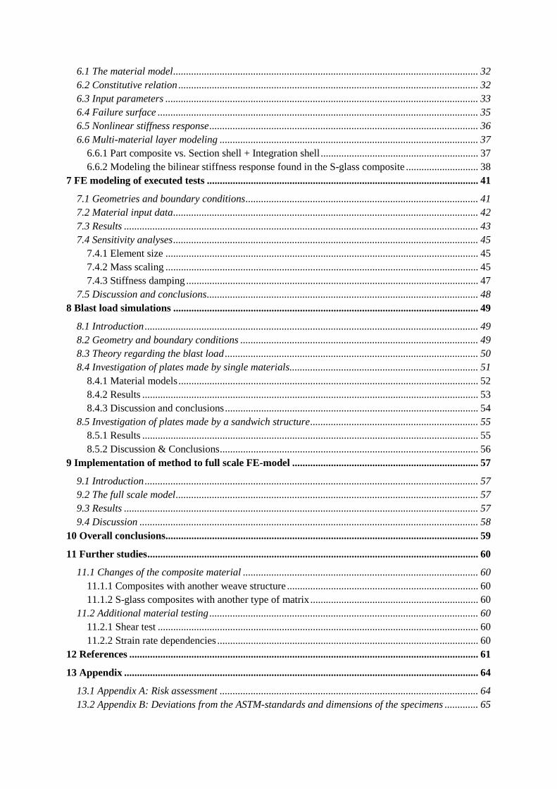
6.1 The material model ...................................................................................................................... 32
6.2 Constitutive relation .................................................................................................................... 32
6.3 Input parameters ......................................................................................................................... 33
6.4 Failure surface ............................................................................................................................ 35
6.5 Nonlinear stiffness response ........................................................................................................ 36
6.6 Multi-material layer modeling .................................................................................................... 37
6.6.1 Part composite vs. Section shell + Integration shell ............................................................. 37
6.6.2 Modeling the bilinear stiffness response found in the S-glass composite ............................ 38
7 FE modeling of executed tests ......................................................................................................... 41
7.1 Geometries and boundary conditions .......................................................................................... 41
7.2 Material input data ...................................................................................................................... 42
7.3 Results ......................................................................................................................................... 43
7.4 Sensitivity analyses ...................................................................................................................... 45
7.4.1 Element size ......................................................................................................................... 45
7.4.2 Mass scaling ......................................................................................................................... 45
7.4.3 Stiffness damping ................................................................................................................. 47
7.5 Discussion and conclusions ......................................................................................................... 48
8 Blast load simulations ...................................................................................................................... 49
8.1 Introduction ................................................................................................................................. 49
8.2 Geometry and boundary conditions ............................................................................................ 49
8.3 Theory regarding the blast load .................................................................................................. 50
8.4 Investigation of plates made by single materials......................................................................... 51
8.4.1 Material models .................................................................................................................... 52
8.4.2 Results .................................................................................................................................. 53
8.4.3 Discussion and conclusions .................................................................................................. 54
8.5 Investigation of plates made by a sandwich structure ................................................................. 55
8.5.1 Results .................................................................................................................................. 55
8.5.2 Discussion & Conclusions .................................................................................................... 56
9 Implementation of method to full scale FE-model ........................................................................ 57
9.1 Introduction ................................................................................................................................. 57
9.2 The full scale model ..................................................................................................................... 57
9.3 Results ......................................................................................................................................... 57
9.4 Discussion ................................................................................................................................... 58
10 Overall conclusions ......................................................................................................................... 59
11 Further studies ................................................................................................................................ 60
11.1 Changes of the composite material ........................................................................................... 60
11.1.1 Composites with another weave structure .......................................................................... 60
11.1.2 S-glass composites with another type of matrix ................................................................. 60
11.2 Additional material testing ........................................................................................................ 60
11.2.1 Shear test ............................................................................................................................ 60
11.2.2 Strain rate dependencies ..................................................................................................... 60
12 References ....................................................................................................................................... 61
13 Appendix ......................................................................................................................................... 64
13.1 Appendix A: Risk assessment .................................................................................................... 64
13.2 Appendix B: Deviations from the ASTM-standards and dimensions of the specimens ............. 65

13.3 Appendix C: Mechanical properties of the fiberglass’s ............................................................ 67
13.4 Appendix D: Information about the epoxy resin ....................................................................... 68
13.5 Appendix E: Explicit vs. implicit time integration algorithms .................................................. 69
13.6 Appendix F: Invariant node numbering .................................................................................... 71
13.7 Appendix G: PART_STIFFNESS ............................................................................................... 73
13.8 Appendix H: Optimizing the flexural stiffness-to-weight ratio .................................................. 74
1
1 Introduction
1.1 Background
British Aerospace (BAE) Systems Hägglunds AB [1], hereinafter called BAE, is a Swedish
incorporated company originally founded by Johan Hägglund in 1899 as a carpentry workshop named
Hägglund & Söner [1]. The company has been involved in several merges and is now a part of the
British concern BAE Systems. Today, BAE is primarily a manufacturer of tracked military ground
vehicles such as the combat vehicle CV90 and the all-terrain vehicle BvS10.
It is of great interest to reduce the weight of the military vehicles manufactured by BAE since it results
in increased vehicle range due to decreased fuel consumption. In addition, reduced vehicle weight
generally improves the mobility and facilitates long-distance transports of the vehicles.
Reducing the weight is a continuous process and is primarily achieved by replacing the materials in
certain components with lighter materials, such as composite/sandwich materials. In components
intended for protection against threats like projectiles and explosive loads, Glass Fiber Reinforced
Polymers (GFRP) are getting more commonly used due to appealing material properties, such as a
high strength-to-weight ratio [2]. Two appealing GFRP-materials are S-glass and E-glass fibers, both
embedded in an epoxy matrix.
1.2 Problem description
Before replacing the material in any component, extensive investigations are necessary to ensure that
the current specification of requirements is fulfilled. This is particularly important for components in
the vehicles protection equipment. The investigations consist of both actual tests and of numerical
simulations where a vehicle is subjected to loads corresponding to specific threats.
Initial Finite Element (FE)-analyses shows that the GFRP-materials appear to be suitable to use in
some of the components intended for protection in the vehicles. Today, generic material data to model
the GFRP-materials is used at BAE, with mechanical properties found in the literature complemented
with assumptions. Results found from analyses based on this method are therefore uncertain. Hence, it
is of interest to investigate a more accurate method, which can be better motivated from a physical
point of view.
1.3 Aim
The aim of this thesis work is to come up with a method to properly model the behavior of the E- and
S-glass composites in LS-DYNA, which is one of the FE-softwares used by BAE. More specifically,
the elastic response, potential plastic flow, damage and failure behaviors are of interest to include in
the method. The input parameters to the FE-model are to be based essentially on mechanical properties
obtained from material testing rather than from literature (since properties found in literature naturally
is associated with uncertainties).
2
1.4 Structure
The project is initiated with a literature survey regarding testing of GFRP-materials, followed by
actual testing of both the S-glass and E-glass composites. A literature survey concerning modeling
GFRP-materials in LS-DYNA is performed and the executed tests are reconstructed in LS-DYNA.
The developed method for modeling the composites is then applied in blast load analyses together
with materials conventionally used as protection. This comparative study will provide a hint about the
GFRP-materials ability to act as protection against blast loads. Finally, the developed method is
applied in an existing FE-model of a BAE manufactured vehicle subjected to a load corresponding to a
specific threat. The results found from these FE-simulations are compared to actual test results as well
as to results found from simulations with the currently used method to model a generic GFRP
material.
The report is divided into two parts, the first part concerns material testing and the second part
contains all work associated with the numerical simulations. At the end of the report, overall
conclusions are presented and recommendations on how to further improve the developed method are
given together with suggestions regarding improvements of the GFRP-materials.
1.5 Delimitations
This project is a 30 credits master thesis extending over 20 weeks. The delimitations applied are
presented below.
The material tests have been limited to quasi-static tensile and flexural tests (due to limited
access to the laboratory). Strain-rate dependencies are not investigated.
The influence of environmental effects on the GFRP-materials will not be investigated in the
material testing (e.g. temperature, moist-level, chemical resistance).
The number of specimens used in the tensile- and flexural tests is restricted.
Only fully implemented material models available in LS-DYNA is considered in the modeling
of the GFRP-materials.
1.6 Other considerations
No gender-related issues are brought up by the work. Nor does it directly relate to issues concerning
the environment or sustainable development of the society. As regards ethical considerations, the work
treats development of armaments and follows Swedish law.

3
Part 1:
Material testing
4
2 Material Testing
2.1 Introduction
2.1.1 Literature survey and preparations The ambition with the literature survey was to improve the authors’ knowledge about tensile and
flexural testing with orthotropic materials, since both the S- and E-glass composite are of such nature.
The literature survey was also intended to increase the awareness of common mistakes and pitfalls.
Several different tutorials of how to execute tensile and flexural tests with orthotropic materials were
found. The most comprehensive ones were provided by the American Society for Testing and
Materials (ASTM). A decision was made to execute both tests in accordance with the corresponding
ASTM-standards, ASTM D3039/D3039M – 00 [3] for the tensile tests and ASTM D7264/D7264M -
07 [4] for the flexural tests.
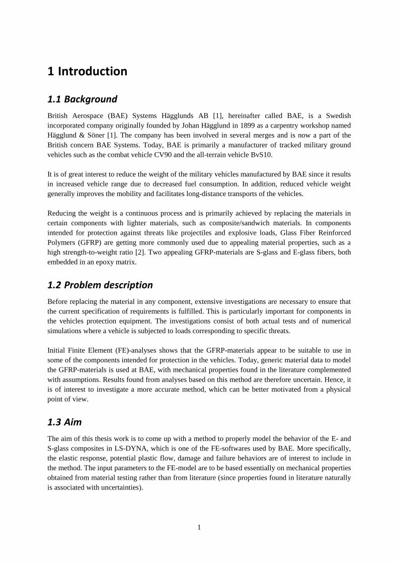
ASTM D3039/D3039M – 00 did not provide any distinct answer to whether or not tabs should be used
in the tensile testing. Tabs are employed to reduce local stress concentrations in the specimens close to
the fixing device, to protect the material from damage caused by the grips of the test machine [5]. A
principal sketch of a specimen with tabs is presented in Figure 1.
Figure 1. Principal sketch of a tensile specimen with tabs.
It was determined that no tabs would be utilized initially. If failure of the specimen occurred close to
the fixing device, tabs would be introduced.
Material testing is always associated with several elements of risk; therefore, a risk assessment was
created prior to the test occasion, presented in Appendix A.
Mean values of the specimens’ thicknesses and widths were calculated based on measurements with a
caliper. The dimensions of each and every specimen are displayed in Appendix B, together with
deviations from the ASTM-standards.
5
2.1.2 S-glass and E-glass S-glass consists of magnesium-aluminosilicate and is generally used as reinforcement in structural
applications that requires high strength and durability under high temperatures and in corrosive
environments. E-glass is comprised of alumina-calcium-borosilicate and is used as reinforcement as
well. It is a high strength fiberglass with a high electrical resistivity.
S-glass is more appropriate in high temperature applications due to a significantly higher glass-liquid
transition temperature. The higher melting point complicates the manufacturing process of the S-glass
fibers which in turn makes the S-glass considerably more expensive than E-glass. [2]
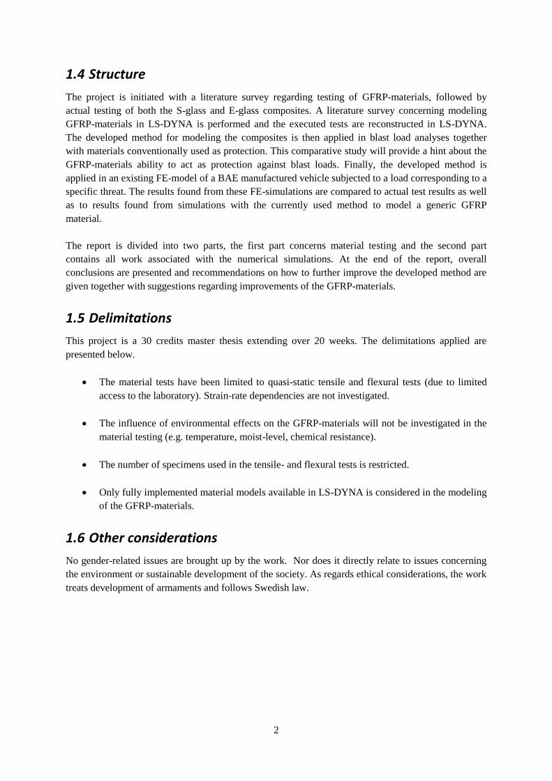
S-glass fibers are superior to E-glass fibers when it comes to the mechanical properties of interest in
general structural applications, which is illustrated in Table 1. The data of the mechanical properties
are gathered from a data sheet provided by the manufacturer of the investigated fiberglass, Owens
Corning [6]. The datasheet is found in Appendix C.
Table 1. Mechanical properties of S- and E-glass fibers gathered from the data sheet presented in Appendix C.
Fiberglass properties Unit S-glass E-glass
Density kg/m3 2450 2550-2580
Ultimate tensile strength MPa 4826-5081 3450-3790
Young’s modulus GPa 88 69-72
Elongation at failure % 5.5 4.8
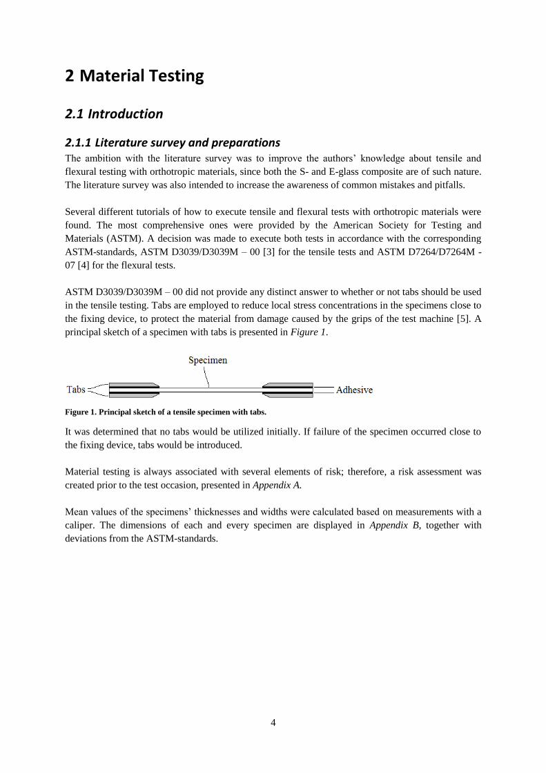
2.1.3 Test specimens The specimens have similar macroscopic structure regardless of the reinforcing fiber type. Plain
fiberglass weave is stacked in the same direction in every layer and the stack is in this case embedded
in an epoxy matrix. A picture of the weave is presented in Figure 2. The mechanical properties of the
weave are the same for every 90 in-plane rotation.
Figure 2. Plain weave consisting of S-glass fibers.
Noteworthy is that the S-glass weave is somewhat denser compared to the E-glass weave. Both the S-
glass and the E-glass specimens are comprised of 65-68 wt.% fiberglass and the same type of epoxy
(Bodopox AF-1200) is used as resin in both specimen types. A product sheet of the epoxy used is
found in Appendix D. The density of the S-glass composite is 1750 kg/m3 and density of the E-glass
composite is 1820 kg/m3.
The specimens are manufactured by the company Nordfarbo [7] and the manufacturing process begins
with stacking of the weave in a certain mold. Epoxy is injected in the mold and the composite is
6
subjected to a pressure reduction, close to a vacuum-state, to reduce the amount of air contained in the
composite. The pressure affected composite is then heated and cured at 60 for 16 hours.
A total of 14 specimens were manufactured for tensile testing whereas 12 specimens were
manufactured for the flexural tests. All of the tensile specimens had a thickness of 6 mm and different
fiber orientations, whereas all the flexural specimens had a fiber orientation of 0°/90° and different
thicknesses. Each type of specimens is assigned a unique ID, where:
S/E refers to the type of reinforcing fiberglass (S-glass or E-glass)
T/F refers to the type of test the specimens are applied in (Tensile or Flexural test).
The following digits refer to either fiber orientation or thickness in/of the specimens.
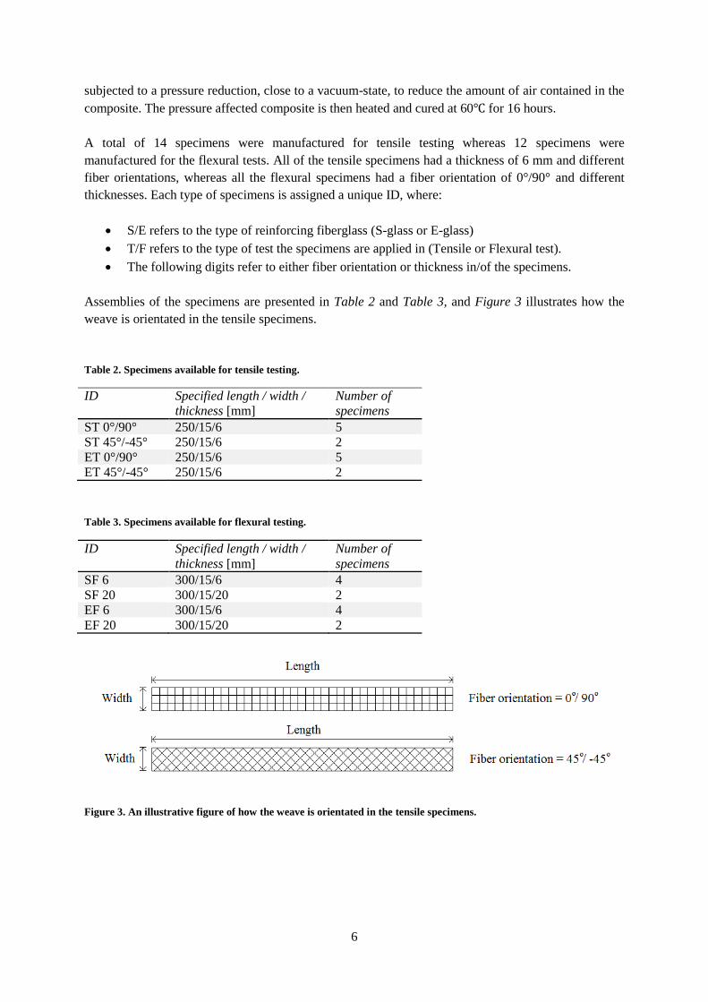
Assemblies of the specimens are presented in Table 2 and Table 3, and Figure 3 illustrates how the
weave is orientated in the tensile specimens.
Table 2. Specimens available for tensile testing.
ID Specified length / width /
thickness [mm]
Number of
specimens
ST 0°/90° 250/15/6 5
ST 45°/-45° 250/15/6 2
ET 0°/90° 250/15/6 5
ET 45°/-45° 250/15/6 2
Table 3. Specimens available for flexural testing.
ID Specified length / width /
thickness [mm]
Number of
specimens
SF 6 300/15/6 4
SF 20 300/15/20 2
EF 6 300/15/6 4
EF 20 300/15/20 2
Figure 3. An illustrative figure of how the weave is orientated in the tensile specimens.
7
3 Tensile testing
3.1 Introduction
The tests were conducted at Linköping University on the 13th, 20
th and 21
st of February 2014. An
experienced machine operator was present during the test occasions to ensure that the testing was safe
and properly executed. The machine utilized was an Instron 5582, calibrated in May 2013 with
expiring date in November 2014. The tensile rate was 1 mm/min and the sampling rate was 10 Hz.
Due to the absence of a neck in the specimens, the gripping area was made as large as possible to
minimize the necessary clamping pressure required to prevent slip between the grips and the specimen.
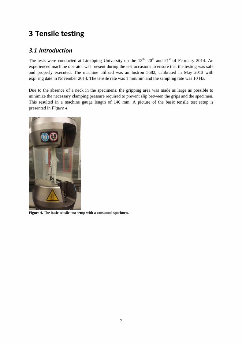
This resulted in a machine gauge length of 140 mm. A picture of the basic tensile test setup is
presented in Figure 4.
Figure 4. The basic tensile test setup with a consumed specimen.
8
3.2 Test methods
3.2.1 Tensile tests without extensometers If the extensometers are attached to the specimen when failure occurs, it is likely that they will be
damaged. Therefore it is preferable to remove the extensometers from the specimens before failure
occurs. In order to succeed with this, an approximate value of the failure load is required.
The ultimate tensile strength is calculated as follows:
⁄ (3.1)
where:
= Ultimate tensile strength [MPa]
= Load at failure [N]
= Initial average cross sectional area [mm2]
3.2.2 Tensile tests with one extensometer The extensometer is attached to the middle of the specimen and measures local axial strain. The strains
found from the extensometer is hereinafter referred to as local strains whereas the strains based on the
test machine’s beam displacement will be referred to as global strains. The beam is the part of the test
machine that moves with the predefined rate, causing tension in the specimen. The local strains
obtained once the extensometer has been removed have no physical meaning and are therefore
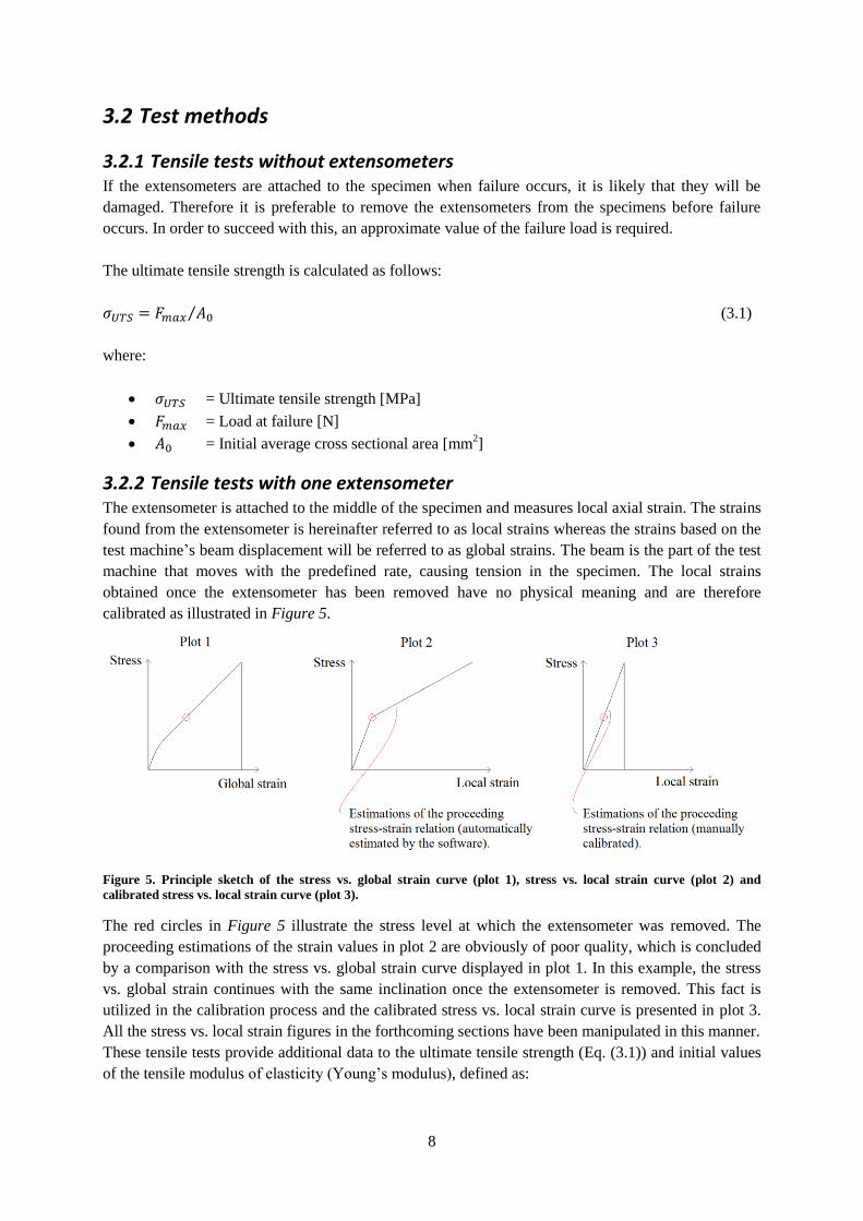
calibrated as illustrated in Figure 5.
Figure 5. Principle sketch of the stress vs. global strain curve (plot 1), stress vs. local strain curve (plot 2) and
calibrated stress vs. local strain curve (plot 3).
The red circles in Figure 5 illustrate the stress level at which the extensometer was removed. The
proceeding estimations of the strain values in plot 2 are obviously of poor quality, which is concluded
by a comparison with the stress vs. global strain curve displayed in plot 1. In this example, the stress
vs. global strain continues with the same inclination once the extensometer is removed. This fact is
utilized in the calibration process and the calibrated stress vs. local strain curve is presented in plot 3.
All the stress vs. local strain figures in the forthcoming sections have been manipulated in this manner.
These tensile tests provide additional data to the ultimate tensile strength (Eq. (3.1)) and initial values
of the tensile modulus of elasticity (Young’s modulus), defined as:
9
(3.2)
where:
= Tensile modulus of elasticity [Pa]
= Difference in tensile stress between two strain points [Pa]
= Difference between two local strain points [-]
The local strain values also enable calculation of the modulus of toughness, UT, which is a measure of
the materials ability to absorb energy, defined as:
∫
(3.3)
where:
UT = Modulus of toughness [J/m3]
= Stress [Pa]
= Local strain [-]
3.2.3 Tensile tests with three extensometers Three extensometers are used simultaneously; one measuring the axial strain and two measuring both
of the transverse strains (the strain over the thickness and the strain over the width). The
extensometers are positioned as close to the middle of the specimens as possible. Besides additional
data of the aforementioned properties obtained by Eq. (3.1), Eq. (3.2) and Eq. (3.3) the Poisson’s
ratios can be determined, according to:
⁄⁄ (3.4)
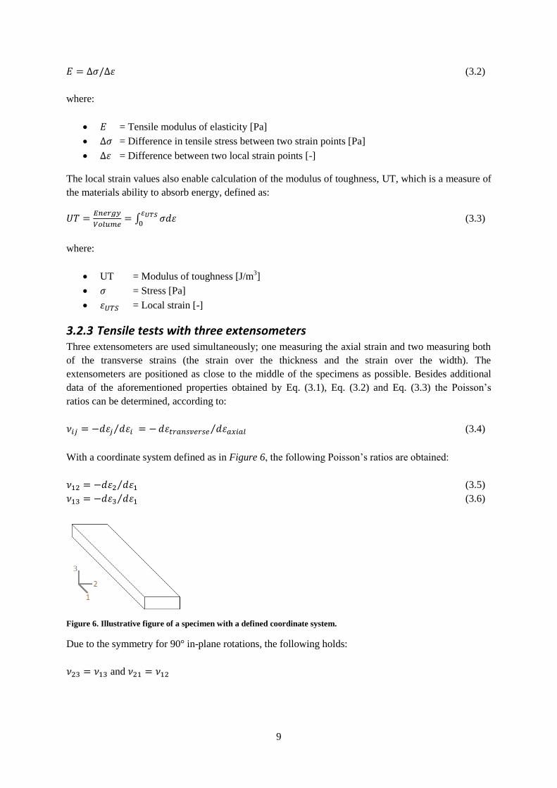
With a coordinate system defined as in Figure 6, the following Poisson’s ratios are obtained:
⁄ (3.5)
⁄ (3.6)
Figure 6. Illustrative figure of a specimen with a defined coordinate system.
Due to the symmetry for 90 in-plane rotations, the following holds:
and
10
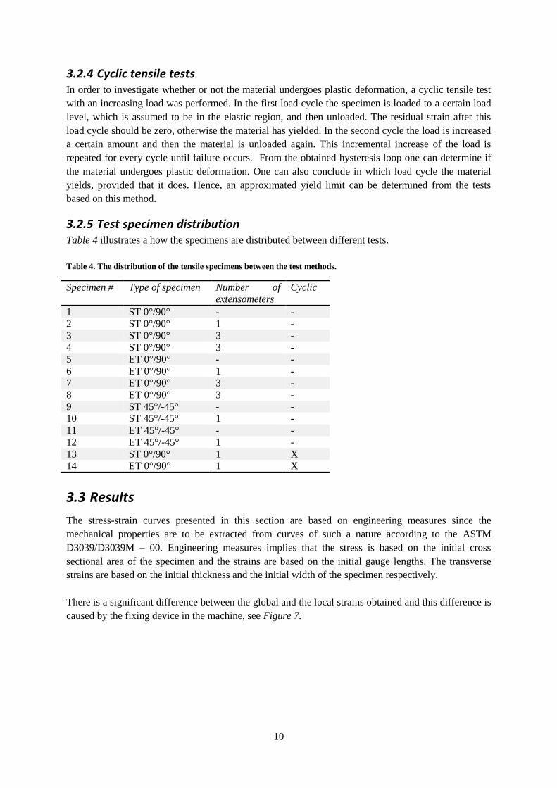
3.2.4 Cyclic tensile tests In order to investigate whether or not the material undergoes plastic deformation, a cyclic tensile test
with an increasing load was performed. In the first load cycle the specimen is loaded to a certain load
level, which is assumed to be in the elastic region, and then unloaded. The residual strain after this
load cycle should be zero, otherwise the material has yielded. In the second cycle the load is increased
a certain amount and then the material is unloaded again. This incremental increase of the load is
repeated for every cycle until failure occurs. From the obtained hysteresis loop one can determine if
the material undergoes plastic deformation. One can also conclude in which load cycle the material
yields, provided that it does. Hence, an approximated yield limit can be determined from the tests
based on this method.
3.2.5 Test specimen distribution Table 4 illustrates a how the specimens are distributed between different tests.
Table 4. The distribution of the tensile specimens between the test methods.
Specimen # Type of specimen Number of
extensometers
Cyclic
1 ST 0°/90° - -
2 ST 0°/90° 1 -
3 ST 0°/90° 3 -
4 ST 0°/90° 3 -
5 ET 0°/90° - -
6 ET 0°/90° 1 -
7 ET 0°/90° 3 -
8 ET 0°/90° 3 -
9 ST 45°/-45° - -
10 ST 45°/-45° 1 -
11 ET 45°/-45° - -
12 ET 45°/-45° 1 -
13 ST 0°/90° 1 X
14 ET 0°/90° 1 X
3.3 Results
The stress-strain curves presented in this section are based on engineering measures since the
mechanical properties are to be extracted from curves of such a nature according to the ASTM
D3039/D3039M – 00. Engineering measures implies that the stress is based on the initial cross
sectional area of the specimen and the strains are based on the initial gauge lengths. The transverse
strains are based on the initial thickness and the initial width of the specimen respectively.
There is a significant difference between the global and the local strains obtained and this difference is
caused by the fixing device in the machine, see Figure 7.
11
Figure 7. Illustrative figure of the machines fixing device.
The fixing device is designed to increase the pressure between the specimen and the grips as the
tensile load increases. This leads to a compression of the specimen’s thickness which results in a beam
displacement greater than the actual extension of the specimen, which suggests that the global strain is
not a representative value of the strain in the specimen. One should also remember that elastic
deformations are present in the test machine as well, but these are presumably negligible in these tests.
The mechanical properties are extracted from the stress vs. local strain curves in accordance with
ASTM D3039/D3039M – 00. The plots of the stress vs. global strain are included even though these
strains are misleading, since they contribute with statistical reliability.
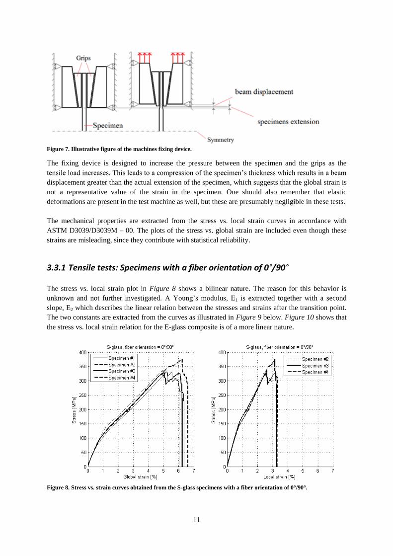
3.3.1 Tensile tests: Specimens with a fiber orientation of 0°/90°
The stress vs. local strain plot in Figure 8 shows a bilinear nature. The reason for this behavior is
unknown and not further investigated. A Young’s modulus, E1 is extracted together with a second
slope, E2 which describes the linear relation between the stresses and strains after the transition point.
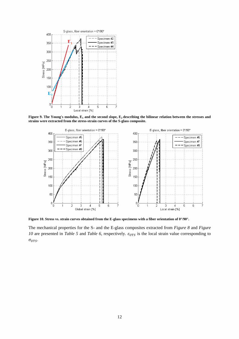
The two constants are extracted from the curves as illustrated in Figure 9 below. Figure 10 shows that
the stress vs. local strain relation for the E-glass composite is of a more linear nature.
Figure 8. Stress vs. strain curves obtained from the S-glass specimens with a fiber orientation of 0°/90°.
12
Figure 9. The Young's modulus, E1 and the second slope, E2 describing the bilinear relation between the stresses and
strains were extracted from the stress-strain curves of the S-glass composite.
Figure 10. Stress vs. strain curves obtained from the E-glass specimens with a fiber orientation of 0°/90°.
The mechanical properties for the S- and the E-glass composites extracted from Figure 8 and Figure
10 are presented in Table 5 and Table 6, respectively. is the local strain value corresponding to
.
13
Table 5. The mechanical properties obtained from the S-glass specimens with a fiber orientation of 0 / 90 based on
the local strain.
[MPa] [%] E1 [GPa] E2 [GPa] UT [MJ/m3]
Specimen #2 336.5 2.50 18.04 11.59 6.08
Specimen #3 329.0 2.61 19.30 9.99 7.09
Specimen #4 376.5 3.16 18.10 10.95 7.48
Sample mean 347.3 2.76 18.48 10.84 6.88
Sample standard
deviation
25.5 0.35 0.71 0.87 0.77
Table 6. The mechanical properties obtained from the E-glass specimens with a fiber orientation of 0 /90 based on
the local strain.
[MPa] [%] E [GPa] UT [MJ/m3]
Specimen #6 359.8 2.30 15.64 4.66
Specimen #7 365.9 2.36 15.50 4.75
Specimen #8 357.5 2.02 17.70 4.09
Sample mean 361.1 2.23 16.28 4.50
Sample standard
deviation
4.3 0.18 1.23 0.36
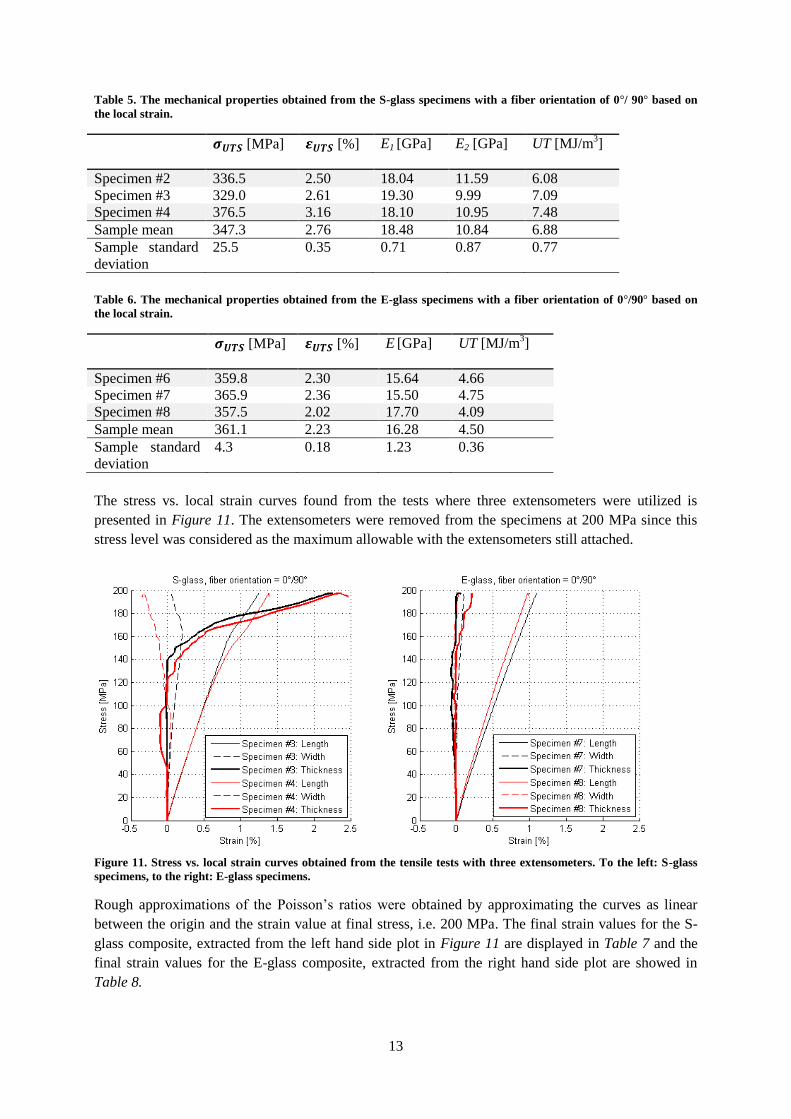
The stress vs. local strain curves found from the tests where three extensometers were utilized is
presented in Figure 11. The extensometers were removed from the specimens at 200 MPa since this
stress level was considered as the maximum allowable with the extensometers still attached.
Figure 11. Stress vs. local strain curves obtained from the tensile tests with three extensometers. To the left: S-glass
specimens, to the right: E-glass specimens.
Rough approximations of the Poisson’s ratios were obtained by approximating the curves as linear
between the origin and the strain value at final stress, i.e. 200 MPa. The final strain values for the S-
glass composite, extracted from the left hand side plot in Figure 11 are displayed in Table 7 and the
final strain values for the E-glass composite, extracted from the right hand side plot are showed in
Table 8.
14
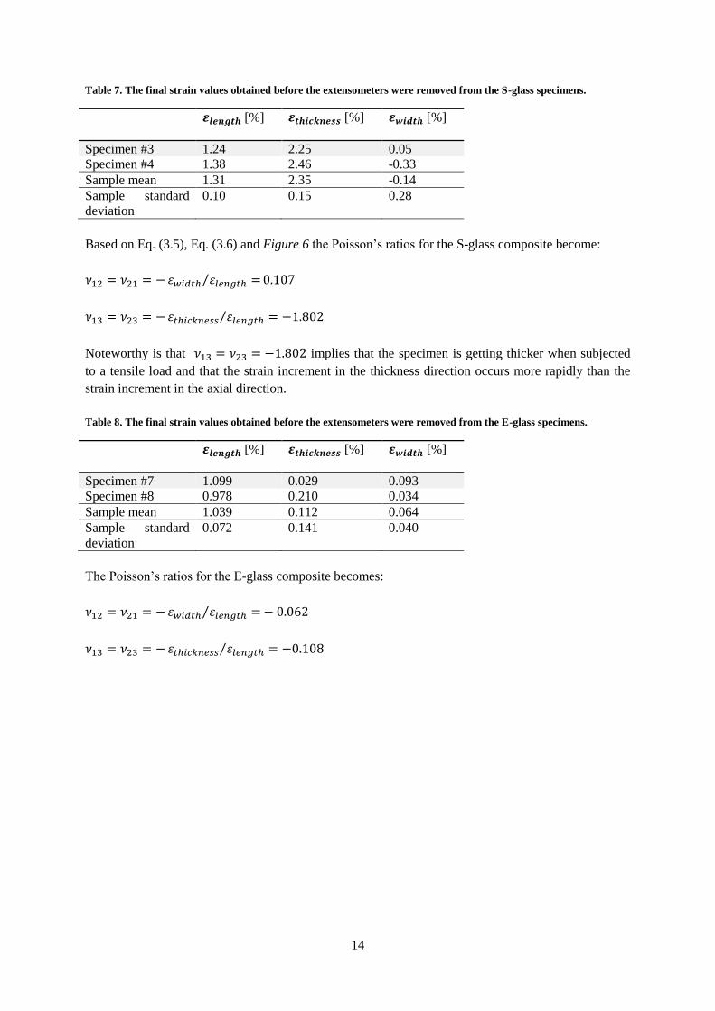
Table 7. The final strain values obtained before the extensometers were removed from the S-glass specimens.
[%] [%] [%]
Specimen #3 1.24 2.25 0.05
Specimen #4 1.38 2.46 -0.33
Sample mean 1.31 2.35 -0.14
Sample standard
deviation
0.10 0.15 0.28
Based on Eq. (3.5), Eq. (3.6) and Figure 6 the Poisson’s ratios for the S-glass composite become:
⁄
⁄
Noteworthy is that implies that the specimen is getting thicker when subjected
to a tensile load and that the strain increment in the thickness direction occurs more rapidly than the
strain increment in the axial direction.
Table 8. The final strain values obtained before the extensometers were removed from the E-glass specimens.
[%] [%] [%]
Specimen #7 1.099 0.029 0.093
Specimen #8 0.978 0.210 0.034
Sample mean 1.039 0.112 0.064
Sample standard
deviation
0.072 0.141 0.040
The Poisson’s ratios for the E-glass composite becomes:
⁄
⁄
15
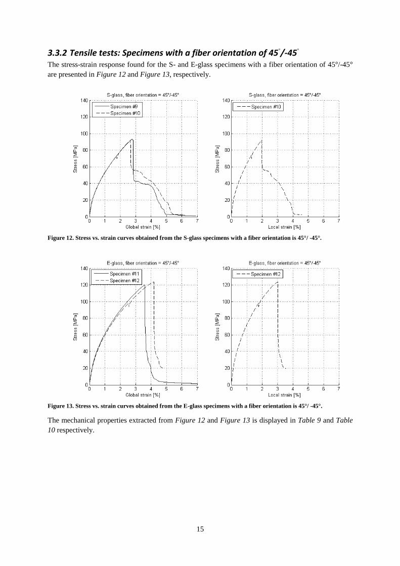
3.3.2 Tensile tests: Specimens with a fiber orientation of 45◦/-45◦ The stress-strain response found for the S- and E-glass specimens with a fiber orientation of 45 /-45
are presented in Figure 12 and Figure 13, respectively.
Figure 12. Stress vs. strain curves obtained from the S-glass specimens with a fiber orientation is 45°/ -45°.
Figure 13. Stress vs. strain curves obtained from the E-glass specimens with a fiber orientation is 45°/ -45°.
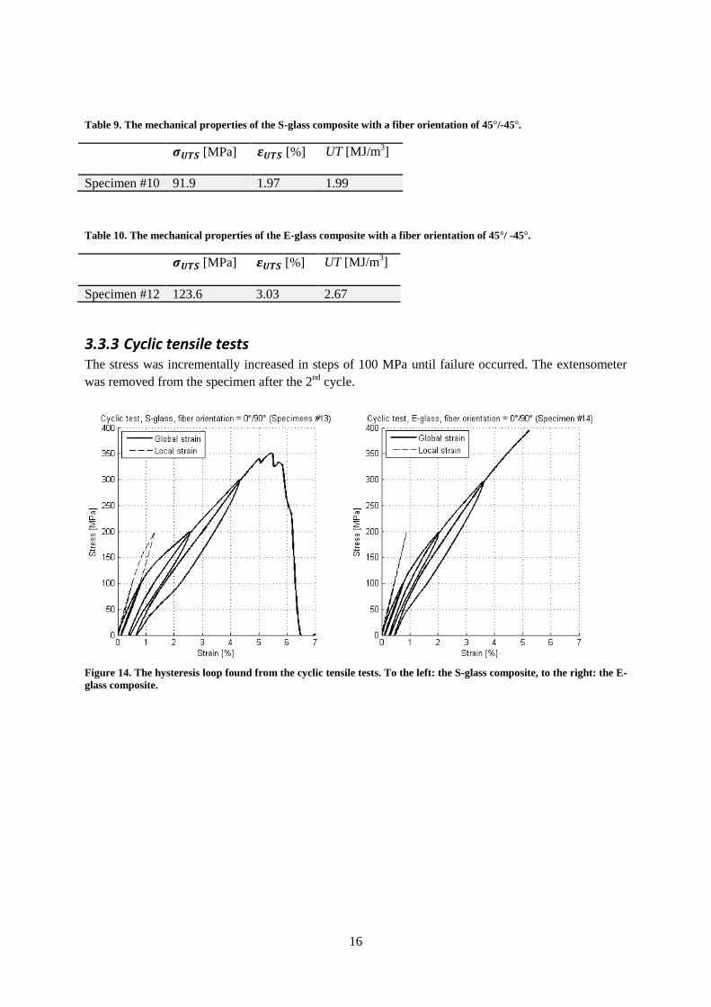
The mechanical properties extracted from Figure 12 and Figure 13 is displayed in Table 9 and Table
10 respectively.
16
Table 9. The mechanical properties of the S-glass composite with a fiber orientation of 45 /-45 .
[MPa] [%] UT [MJ/m3]
Specimen #10 91.9 1.97 1.99
Table 10. The mechanical properties of the E-glass composite with a fiber orientation of 45 / -45 .
[MPa] [%] UT [MJ/m3]
Specimen #12 123.6 3.03 2.67
3.3.3 Cyclic tensile tests The stress was incrementally increased in steps of 100 MPa until failure occurred. The extensometer
was removed from the specimen after the 2nd
cycle.
Figure 14. The hysteresis loop found from the cyclic tensile tests. To the left: the S-glass composite, to the right: the E-
glass composite.
17
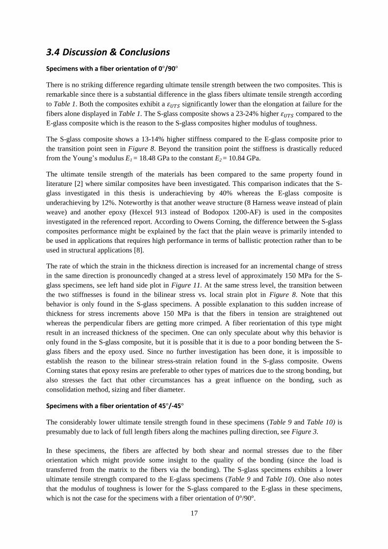
3.4 Discussion & Conclusions
Specimens with a fiber orientation of 0 /90
There is no striking difference regarding ultimate tensile strength between the two composites. This is
remarkable since there is a substantial difference in the glass fibers ultimate tensile strength according
to Table 1. Both the composites exhibit a significantly lower than the elongation at failure for the
fibers alone displayed in Table 1. The S-glass composite shows a 23-24% higher compared to the
E-glass composite which is the reason to the S-glass composites higher modulus of toughness.
The S-glass composite shows a 13-14% higher stiffness compared to the E-glass composite prior to
the transition point seen in Figure 8. Beyond the transition point the stiffness is drastically reduced
from the Young’s modulus E1 = 18.48 GPa to the constant E2 = 10.84 GPa.
The ultimate tensile strength of the materials has been compared to the same property found in
literature [2] where similar composites have been investigated. This comparison indicates that the S-
glass investigated in this thesis is underachieving by 40% whereas the E-glass composite is
underachieving by 12%. Noteworthy is that another weave structure (8 Harness weave instead of plain
weave) and another epoxy (Hexcel 913 instead of Bodopox 1200-AF) is used in the composites
investigated in the referenced report. According to Owens Corning, the difference between the S-glass
composites performance might be explained by the fact that the plain weave is primarily intended to
be used in applications that requires high performance in terms of ballistic protection rather than to be
used in structural applications [8].
The rate of which the strain in the thickness direction is increased for an incremental change of stress
in the same direction is pronouncedly changed at a stress level of approximately 150 MPa for the S-
glass specimens, see left hand side plot in Figure 11. At the same stress level, the transition between
the two stiffnesses is found in the bilinear stress vs. local strain plot in Figure 8. Note that this
behavior is only found in the S-glass specimens. A possible explanation to this sudden increase of
thickness for stress increments above 150 MPa is that the fibers in tension are straightened out
whereas the perpendicular fibers are getting more crimped. A fiber reorientation of this type might
result in an increased thickness of the specimen. One can only speculate about why this behavior is
only found in the S-glass composite, but it is possible that it is due to a poor bonding between the S-
glass fibers and the epoxy used. Since no further investigation has been done, it is impossible to
establish the reason to the bilinear stress-strain relation found in the S-glass composite. Owens
Corning states that epoxy resins are preferable to other types of matrices due to the strong bonding, but
also stresses the fact that other circumstances has a great influence on the bonding, such as
consolidation method, sizing and fiber diameter.
Specimens with a fiber orientation of 45 /-45
The considerably lower ultimate tensile strength found in these specimens (Table 9 and Table 10) is
presumably due to lack of full length fibers along the machines pulling direction, see Figure 3.
In these specimens, the fibers are affected by both shear and normal stresses due to the fiber
orientation which might provide some insight to the quality of the bonding (since the load is
transferred from the matrix to the fibers via the bonding). The S-glass specimens exhibits a lower
ultimate tensile strength compared to the E-glass specimens (Table 9 and Table 10). One also notes
that the modulus of toughness is lower for the S-glass compared to the E-glass in these specimens,
which is not the case for the specimens with a fiber orientation of 0 /90 .

18
Cyclic tensile tests
There are residual strains after unloading the material, as displayed in Figure 14. The reason for this is
however not investigated. One notes that the curves demonstrate a hysteresis, which implies that the
material is not purely elastic.
Conclusions:
The composites perform equally in terms of ultimate tensile strength.
The S-glass composite outperforms the E-glass composite in terms of ability to absorb energy.
There is a difference between the stiffness responses for the two composites. The reason is not
investigated due to a limited amount of time.
19
4 Flexural tests
4.1 Introduction
The tests were conducted at Linköping University on the 13th, 20
th and 21
st of February 2014. All of
the conducted flexural tests were of a three point bending nature, with a support span of 180 mm. This
implies a support span-to-thickness ratio of 30:1 for the specimens with a thickness of 6 mm and a
support span-to-thickness ratio of 9:1 for the specimens with 20 mm thickness. Worth mentioning is
that the thicker specimens do not comply with the ASTM D7264/D7264M – 07 recommendations
regarding the support span-to-thickness ratio. According to the standard, a ratio of at least 12:1 should
be fulfilled in order to minimize the influence of shearing.
Both the punch and the supports were of cylindrical shape with a radius of 30 mm instead of 3 mm,
which is the recommended dimensions in ASTM D7264/D7264M – 07.
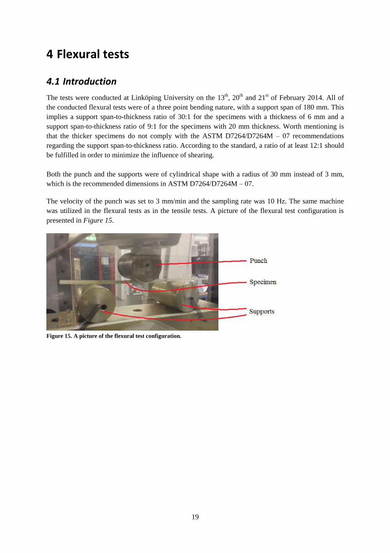
The velocity of the punch was set to 3 mm/min and the sampling rate was 10 Hz. The same machine
was utilized in the flexural tests as in the tensile tests. A picture of the flexural test configuration is
presented in Figure 15.
Figure 15. A picture of the flexural test configuration.
20
4.2 Test methods
4.2.1 Basic flexural tests The flexural test is straightforward; the specimen is placed and aligned on the supports and then the
test is executed. The mechanical properties obtained are based on Euler-Bernoulli beam theory, all in
accordance with ASTM D7264/D7264M – 07.
Flexural strength: ⁄ (4.1)
where:
= Stress at the outer surface under the punch [MPa]
= Maximum applied force [N]
= Support span [mm]
= Width of the beam [mm]
= Thickness of the beam [mm]
Maximum strain: ⁄ (4.2)
where:
= Maximum strain at the outer surface [-]
= Deflection of the beam [m]
Flexural modulus of elasticity: ⁄ (4.3)
where:
= Flexural modulus of elasticity [Pa]
= Difference in flexural stress between two selected points [Pa]
= Difference between two selected strain points [-]
4.2.2 Cyclic flexural tests This method is similar to the one presented in “3.2.4 Cyclic tensile test” and contributes with
additional data of the aforementioned mechanical properties obtained by Eq. (4.1), Eq. (4.2) and Eq.
(4.3) as well as information about the potential plastic behavior of the composites.
The distribution of the specimens between the two test methods is showed in Table 11.
21
Table 11. The distribution of the flexural test specimens between the two test methods.
Specimen # Type of specimen Basic flexural test Cyclic
1 SF 6 X -
2 SF 6 X -
3 EF 6 X -
4 EF 6 X -
5 SF 20 X -
6 SF 20 X -
7 EF 20 X -
8 EF 20 X -
9 SF 6 - X
10 SF 6 - X
11 EF 6 - X
12 EF 6 - X
4.3 Results
The results consist of figures of load vs. deflection and tables with the extracted mechanical properties.
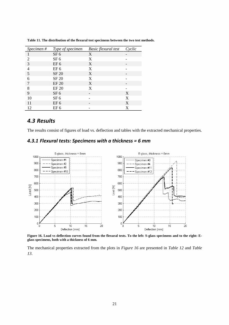
4.3.1 Flexural tests: Specimens with a thickness = 6 mm
Figure 16. Load vs deflection curves found from the flexural tests. To the left: S-glass specimens and to the right: E-
glass specimens, both with a thickness of 6 mm.
The mechanical properties extracted from the plots in Figure 16 are presented in Table 12 and Table
13.
22
Table 12. Mechanical properties obtained from the flexural tests of the S-glass specimens with a thickness of 6 mm.
[MPa] [%] [GPa]
Specimen #1 233.2 1.12 23.06
Specimen #2 268.7 1.21 23.34
Specimen #9 266.0 1.16 23.48
Specimen #10 251.8 1.13 23.92
Sample mean
Sample standard deviation
254.9
16.3
1.16
0.04
23.45
0.36
Table 13. Mechanical properties obtained from the flexural tests of the E-glass specimens with a thickness of 6 mm.
[MPa] [%] [GPa]
Specimen #3 344.5 1.42 24.40
Specimen #4 467.4 1.91 25.35
Specimen #11 348.3 1.46 24.75
Specimen #12 418.5 1.75 24.61
Sample mean
Sample standard deviation
394.7
59.2
1.64
0.24
24.78
0.41
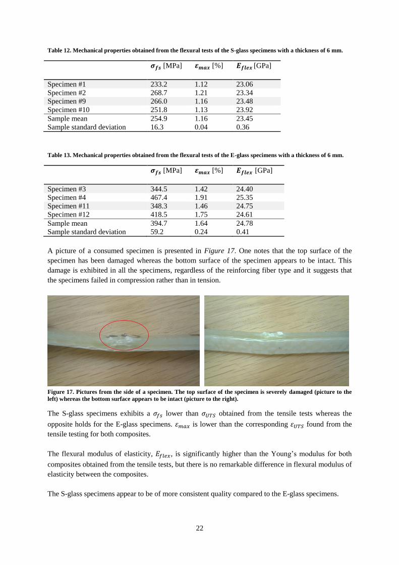
A picture of a consumed specimen is presented in Figure 17. One notes that the top surface of the
specimen has been damaged whereas the bottom surface of the specimen appears to be intact. This
damage is exhibited in all the specimens, regardless of the reinforcing fiber type and it suggests that
the specimens failed in compression rather than in tension.
Figure 17. Pictures from the side of a specimen. The top surface of the specimen is severely damaged (picture to the
left) whereas the bottom surface appears to be intact (picture to the right).
The S-glass specimens exhibits a lower than obtained from the tensile tests whereas the
opposite holds for the E-glass specimens. is lower than the corresponding found from the
tensile testing for both composites.
The flexural modulus of elasticity, , is significantly higher than the Young’s modulus for both
composites obtained from the tensile tests, but there is no remarkable difference in flexural modulus of
elasticity between the composites.
The S-glass specimens appear to be of more consistent quality compared to the E-glass specimens.
23
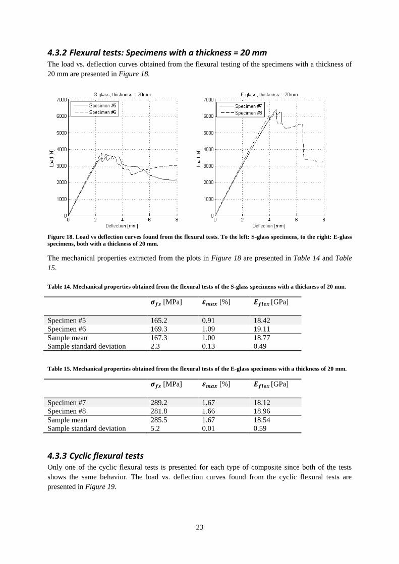
4.3.2 Flexural tests: Specimens with a thickness = 20 mm The load vs. deflection curves obtained from the flexural testing of the specimens with a thickness of
20 mm are presented in Figure 18.
Figure 18. Load vs deflection curves found from the flexural tests. To the left: S-glass specimens, to the right: E-glass
specimens, both with a thickness of 20 mm.
The mechanical properties extracted from the plots in Figure 18 are presented in Table 14 and Table
15.
Table 14. Mechanical properties obtained from the flexural tests of the S-glass specimens with a thickness of 20 mm.
[MPa] [%] [GPa]
Specimen #5 165.2 0.91 18.42
Specimen #6 169.3 1.09 19.11
Sample mean
Sample standard deviation
167.3
2.3
1.00
0.13
18.77
0.49
Table 15. Mechanical properties obtained from the flexural tests of the E-glass specimens with a thickness of 20 mm.
[MPa] [%] [GPa]
Specimen #7 289.2 1.67 18.12
Specimen #8 281.8 1.66 18.96
Sample mean
Sample standard deviation
285.5
5.2
1.67
0.01
18.54
0.59
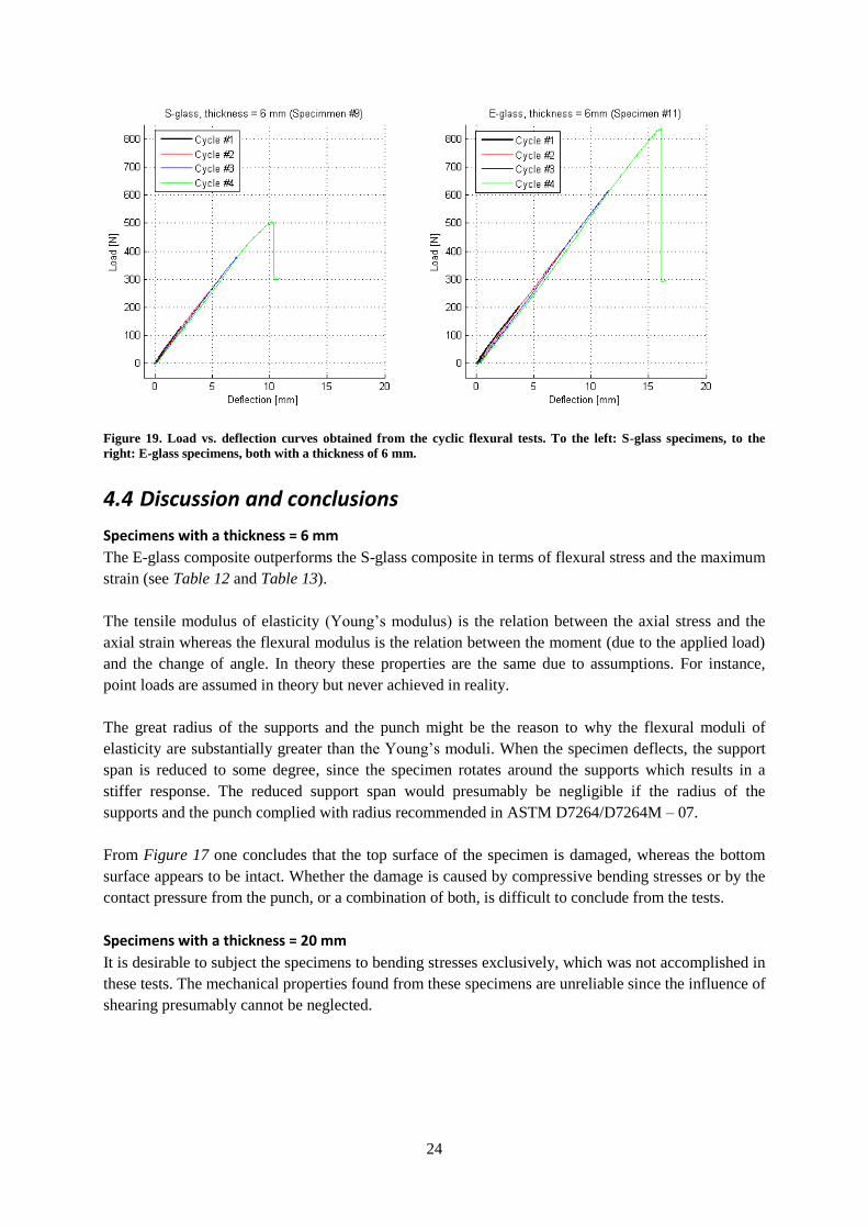
4.3.3 Cyclic flexural tests Only one of the cyclic flexural tests is presented for each type of composite since both of the tests
shows the same behavior. The load vs. deflection curves found from the cyclic flexural tests are
presented in Figure 19.
24
Figure 19. Load vs. deflection curves obtained from the cyclic flexural tests. To the left: S-glass specimens, to the
right: E-glass specimens, both with a thickness of 6 mm.
4.4 Discussion and conclusions
Specimens with a thickness = 6 mm
The E-glass composite outperforms the S-glass composite in terms of flexural stress and the maximum
strain (see Table 12 and Table 13).
The tensile modulus of elasticity (Young’s modulus) is the relation between the axial stress and the
axial strain whereas the flexural modulus is the relation between the moment (due to the applied load)
and the change of angle. In theory these properties are the same due to assumptions. For instance,
point loads are assumed in theory but never achieved in reality.
The great radius of the supports and the punch might be the reason to why the flexural moduli of
elasticity are substantially greater than the Young’s moduli. When the specimen deflects, the support
span is reduced to some degree, since the specimen rotates around the supports which results in a
stiffer response. The reduced support span would presumably be negligible if the radius of the
supports and the punch complied with radius recommended in ASTM D7264/D7264M – 07.
From Figure 17 one concludes that the top surface of the specimen is damaged, whereas the bottom
surface appears to be intact. Whether the damage is caused by compressive bending stresses or by the
contact pressure from the punch, or a combination of both, is difficult to conclude from the tests.
Specimens with a thickness = 20 mm
It is desirable to subject the specimens to bending stresses exclusively, which was not accomplished in
these tests. The mechanical properties found from these specimens are unreliable since the influence of
shearing presumably cannot be neglected.

25
Cyclic flexural tests
There are no signs of plastic deformation in these cyclic tests, see Figure 19. Based on the curves, it
may be concluded that the material demonstrates an elastic behavior.
Conclusions:
The E-glass composite outperforms the S-glass composite in terms of both and .
The failure of the specimens with a thickness of 6 mm appears on the upper surface.

26
Part 2:
Numerical simulations
27
5 Numerical methods
5.1 Introduction
The aim with this part of the thesis is to develop a method to model both of the composites in LS-
DYNA. The GFRP-materials will be modeled as homogeneous materials since this simplifies the
modeling work significantly, i.e. the glass fiber and the epoxy matrix are treated as a continuum. This
assumption is motivated by the fact that the GFRP-materials consist of 65-68 wt.% fiberglass
regardless of the composites thickness.
A decision was made to model the composites as exclusively elastic which also is an assumption made
to simplify the modeling work. This is a pragmatic approach to model the complex behavior found in
the material testing.
All the numerical simulations in this and forthcoming sections are solved with explicit time
integration. The difference between the explicit time integration algorithm and the more
conventionally used implicit time integration algorithm is explained in Appendix E.
28
5.2 Survey of material models in LS-DYNA
LS-DYNA contains numerous of material models suitable for modeling orthotropic materials. It is
preferable to exclude inappropriate material models at an early stage in order to avoid unnecessary
simulation work. The purpose with this literature survey was to gather information about all the
available material models capable of dealing with orthotropic materials. Information was primarily
gathered from the LS-DYNA Keyword manual vol. II [9] and the LS-DYNA Theory manual [10].
Material models requiring additional licenses were rejected directly together with models known for
exhibiting numerical instabilities according to the LS-DYNA keyword manual vol. II [9]. Material
models intended to model specific materials with poor resemblance to the GFRP-materials were also
excluded. The following material models remained:
MAT002 – ORTHOTROPIC_ELASTIC
MAT022 – COMPOSITE_DAMAGE
MAT023 – TEMPERATURE_DEPENDENT_ORTHOTROPIC
MAT054 – ENHANCED_COMPOSITE_DAMAGE (failure criteria according to Chang and Chang)
MAT055 – EHHANCED_COMPOSITE_DAMAGE (failure criteria according to Tsai and Wu)
MAT058 – LAMINATED_COMPOSITE_FABRIC
MAT059 – COMPOSITE_FAILURE
MAT108 – ORTHO_ELASTIC_PLASTIC
MAT157 – ANISOTROPIC_ELASTIC_PLASTIC
MAT158 – RATE_SENSITIVE_COMPOSITE_FABRIC
MAT221 – ORTHOTROPIC_SIMPLIFIED_DAMAGE
A specification of the desirable features was formed to find the most suitable of the material models
listed. The material model:
Should include failure.
Must be compatible with shell elements.
Should be intended to model composites based on fabric rather than unidirectional composites.
Should capture a nonlinear stress-strain response as the one found for both the composites
with a fiber orientation of 45 /-45 .
Two material models which fulfill the specification presented above were found:
MAT058 – LAMINATED_COMPOSITE_FABRIC
MAT158 – RATE_SENSITIVE_COMPOSITE_FABRIC
The only difference between the two models is that the latter have the possibility to include strain-rate
dependencies. [11] No rate-effects are investigated in this study; hence MAT058 was selected for
further investigation.
29
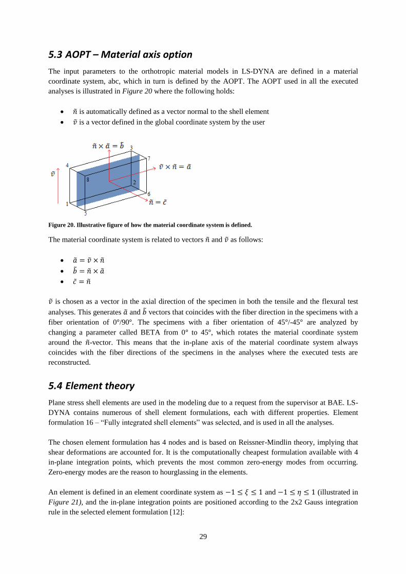
5.3 AOPT – Material axis option
The input parameters to the orthotropic material models in LS-DYNA are defined in a material
coordinate system, abc, which in turn is defined by the AOPT. The AOPT used in all the executed
analyses is illustrated in Figure 20 where the following holds:
is automatically defined as a vector normal to the shell element
is a vector defined in the global coordinate system by the user
Figure 20. Illustrative figure of how the material coordinate system is defined.
The material coordinate system is related to vectors and as follows:
is chosen as a vector in the axial direction of the specimen in both the tensile and the flexural test
analyses. This generates and vectors that coincides with the fiber direction in the specimens with a
fiber orientation of 0 /90 . The specimens with a fiber orientation of 45 /-45 are analyzed by
changing a parameter called BETA from 0 to 45 , which rotates the material coordinate system
around the -vector. This means that the in-plane axis of the material coordinate system always
coincides with the fiber directions of the specimens in the analyses where the executed tests are
reconstructed.
5.4 Element theory
Plane stress shell elements are used in the modeling due to a request from the supervisor at BAE. LS-
DYNA contains numerous of shell element formulations, each with different properties. Element
formulation 16 – “Fully integrated shell elements” was selected, and is used in all the analyses.
The chosen element formulation has 4 nodes and is based on Reissner-Mindlin theory, implying that
shear deformations are accounted for. It is the computationally cheapest formulation available with 4
in-plane integration points, which prevents the most common zero-energy modes from occurring.
Zero-energy modes are the reason to hourglassing in the elements.
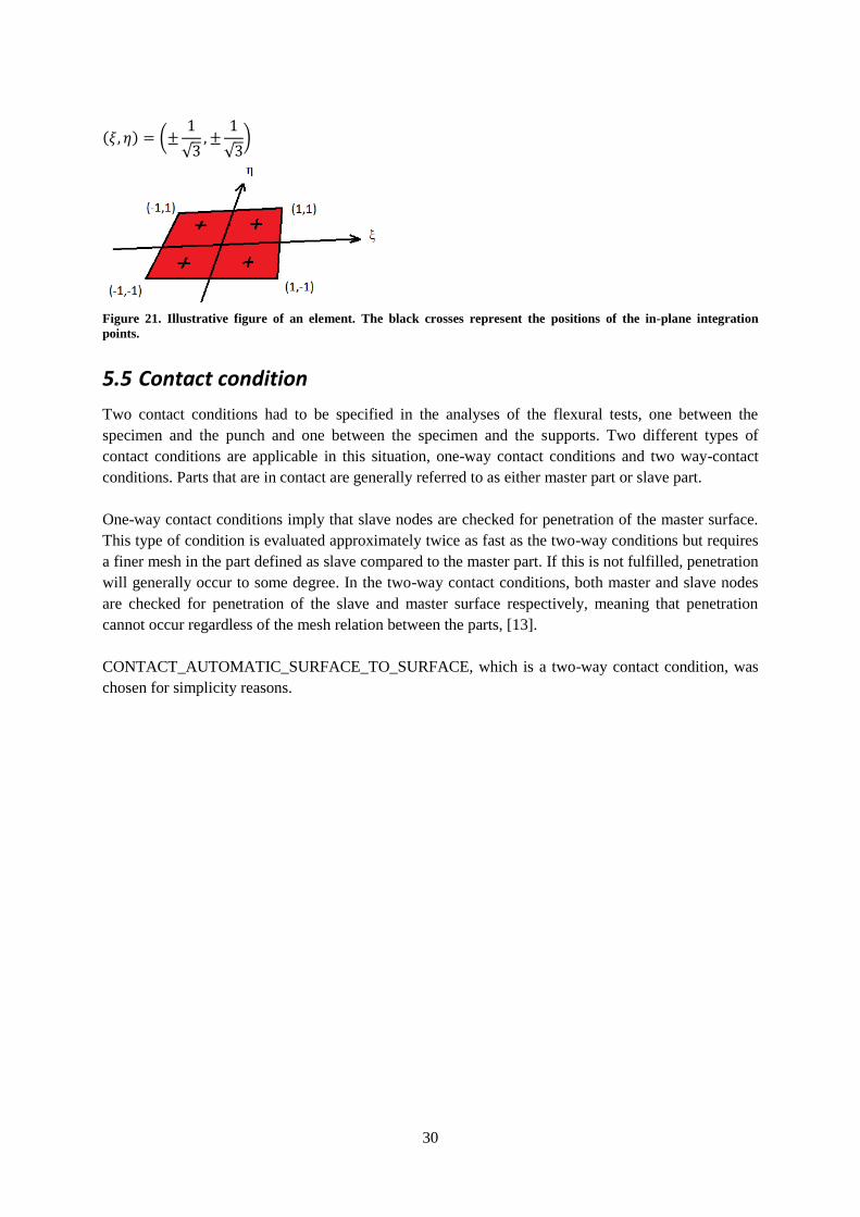
An element is defined in an element coordinate system as and (illustrated in
Figure 21), and the in-plane integration points are positioned according to the 2x2 Gauss integration
rule in the selected element formulation [12]:
30
( ) (
√
√ )
Figure 21. Illustrative figure of an element. The black crosses represent the positions of the in-plane integration
points.
5.5 Contact condition
Two contact conditions had to be specified in the analyses of the flexural tests, one between the
specimen and the punch and one between the specimen and the supports. Two different types of
contact conditions are applicable in this situation, one-way contact conditions and two way-contact
conditions. Parts that are in contact are generally referred to as either master part or slave part.
One-way contact conditions imply that slave nodes are checked for penetration of the master surface.
This type of condition is evaluated approximately twice as fast as the two-way conditions but requires
a finer mesh in the part defined as slave compared to the master part. If this is not fulfilled, penetration
will generally occur to some degree. In the two-way contact conditions, both master and slave nodes
are checked for penetration of the slave and master surface respectively, meaning that penetration
cannot occur regardless of the mesh relation between the parts, [13].
CONTACT_AUTOMATIC_SURFACE_TO_SURFACE, which is a two-way contact condition, was
chosen for simplicity reasons.
31
5.6 Mass scaling
Since the numerical simulations are carried out according to an explicit time integration scheme, mass
scaling has been employed to reduce the CPU-time (which is the time required for an analysis). Mass
scaling is achieved by increasing the density of the materials in the simulations which leads to a larger
time step size according to the CFL-condition, see Appendix E. Greater time step size results in a
reduced CPU-time, since fewer calculations are executed.
A larger mass scaling was applied in the reconstruction of the executed tests since these are of a quasi-
static nature. An investigation of the mass scaling influence was performed for one of the tensile test
simulations and one of the flexural test simulations. Mass scaling is not applied in the other analyses
since the dynamic effects cannot be neglected.
5.7 Additional features used in LS-DYNA
Invariant node numbering (INN) was applied to all simulations to ensure that the results are
independent of the way the nodes are numbered in the elements. A description of INN is found in
Appendix F.
PART_STIFFNESS was applied in the analyses to reduce noise and numerical instabilities. This
feature generates a non-physical damping matrix which affects the results of the analyses to some
degree. Hence the influence of PART_STIFFNESS has been investigated in the simulations where it
has been applied. A short explanation of PART_STIFFNESS is given in Appendix G.
32
6 Material modeling
6.1 The material model
The material model MAT058 – LAMINATED_COMPOSITE_FABRIC is used in all the simulations
and will be the one referred to exclusively hereinafter, even though all the facts presented regarding
this material model holds for MAT158 – RATE_SENSITIVE_COMPOSITE_FABRIC as well.
6.2 Constitutive relation
The stress-strain relation for a linear elastic material, regardless the level of anisotropy, can be
expressed as:
(6.1)
where:
is a 6x1 matrix containing the strains.
is the 6x6 compliance matrix (the inverse of the stiffness matrix).
is a 6x1 matrix containing the stresses.
MAT058 is a linear elastic material model based on orthotropic symmetry. The constitutive relation
(Hooke’s law) utilized is presented in Eq. (6.2).
[
]
[
]
[
]
(6.2)
where the engineering shear strains are related to the corresponding tensor components according to:
(6.3)
One notes that the compliance matrix for an orthotropic material contains 12 material parameters: 3
Young’s moduli, 6 Poisson ratios and 3 shear moduli. However, is symmetric which implies the
following:
33
(6.4)
(6.5)
(6.6)
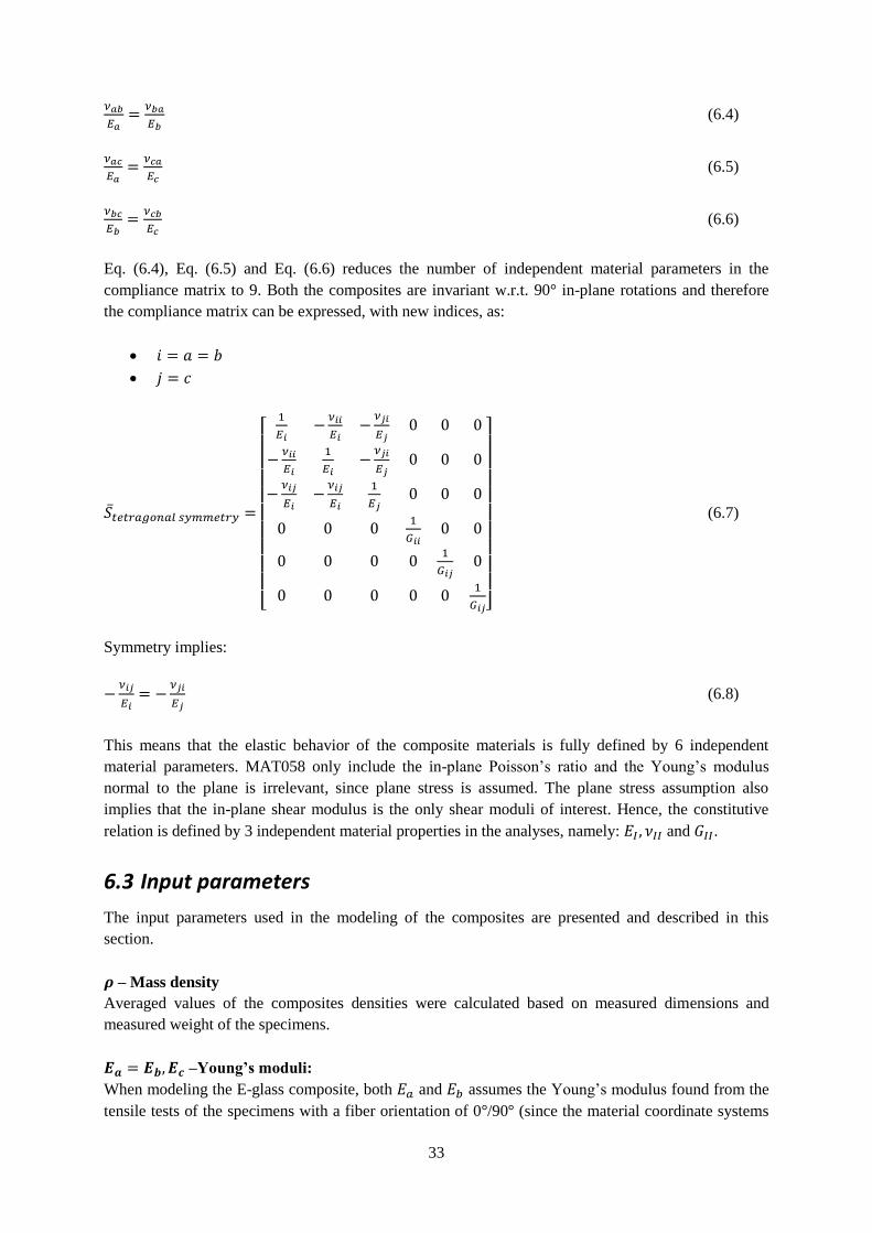
Eq. (6.4), Eq. (6.5) and Eq. (6.6) reduces the number of independent material parameters in the
compliance matrix to 9. Both the composites are invariant w.r.t. 90° in-plane rotations and therefore
the compliance matrix can be expressed, with new indices, as:
[
]
(6.7)
Symmetry implies:
(6.8)
This means that the elastic behavior of the composite materials is fully defined by 6 independent
material parameters. MAT058 only include the in-plane Poisson’s ratio and the Young’s modulus
normal to the plane is irrelevant, since plane stress is assumed. The plane stress assumption also
implies that the in-plane shear modulus is the only shear moduli of interest. Hence, the constitutive
relation is defined by 3 independent material properties in the analyses, namely: and .
6.3 Input parameters
The input parameters used in the modeling of the composites are presented and described in this
section.
– Mass density
Averaged values of the composites densities were calculated based on measured dimensions and
measured weight of the specimens.
–Young’s moduli:
When modeling the E-glass composite, both and assumes the Young’s modulus found from the
tensile tests of the specimens with a fiber orientation of 0 /90 (since the material coordinate systems
34
in-plane axes coincide with the fibers in the specimens). The tensile modulus of elasticity is chosen
rather than the flexural modulus of elasticity since it is more conservative because it leads to larger
deformations, which is due to the lower stiffness. is not used since plane stress prevails in shell
elements.
and for the S-glass composite are determined in “6.6.2 Modeling the bilinear stiffness response
found in the S-glass composite”.
– Shear moduli:
Since no shear testing has been performed, the value of is taken from literature [14], [15]. and
are irrelevant due to the plane stress assumption.
– In-plane Poisson’s ratio:
The in-plane Poisson’s ratios are assigned the values found from the tensile tests of the specimens with
a fiber orientation of 0 /90 according to Eq. (3.5). This holds for both the composite materials.
– Ultimate compressive strengths:
No compression test has been conducted. However, it was observed that the specimens consumed in
the flexural tests failed in compression rather than in tension. These parameters are therefore adjusted
based on inverse modeling of the flexural tests.
– Ultimate tensile strengths:
The ultimate tensile strength obtained from the tensile testing of the specimens with a fiber orientation
of 0 /90 is used as input for the E-glass composite. Two individual tensile strengths were utilized
when modeling the S-glass composite for reasons described in “6.6.2 Modeling the bilinear stiffness
response found in the S-glass composite”.
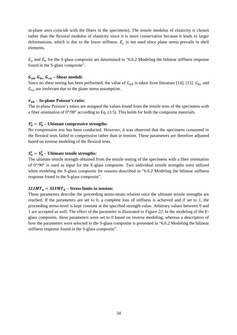
– Stress limits in tension:
These parameters describe the proceeding stress-strain relation once the ultimate tensile strengths are
reached. If the parameters are set to 0, a complete loss of stiffness is achieved and if set to 1, the
proceeding stress-level is kept constant at the specified strength value. Arbitrary values between 0 and
1 are accepted as well. The effect of the parameter is illustrated in Figure 22. In the modeling of the E-
glass composite, these parameters were set to 0 based on inverse modeling, whereas a description of
how the parameters were selected in the S-glass composite is presented in “6.6.2 Modeling the bilinear
stiffness response found in the S-glass composite”.
35
Figure 22. Illustrative figure of how the SLIMT-parameter affects a generic stress-strain curve.
– Stress limits in compression:
These parameters correspond to the SLIMT parameters in compression and are utilized to model the
materials ability to carry load once the compressive strength is reached in the flexural tests. The values
of these parameters are determined by inverse modeling of the flexural tests.
Additional input parameters used are presented and explained in “6.5 Nonlinear stiffness response”
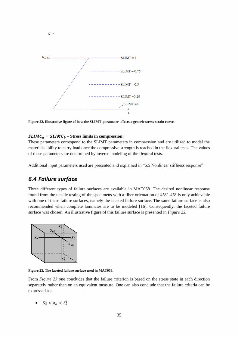
6.4 Failure surface
Three different types of failure surfaces are available in MAT058. The desired nonlinear response
found from the tensile testing of the specimens with a fiber orientation of 45°/ -45° is only achievable
with one of these failure surfaces, namely the faceted failure surface. The same failure surface is also
recommended when complete laminates are to be modeled [16]. Consequently, the faceted failure
surface was chosen. An illustrative figure of this failure surface is presented in Figure 23.
Figure 23. The faceted failure surface used in MAT058.
From Figure 23 one concludes that the failure criterion is based on the stress state in each direction
separately rather than on an equivalent measure. One can also conclude that the failure criteria can be
expressed as:
36
| |
Failure is obtained as soon as any of the conditions above are violated. Whether or not a faceted failure
surface gives the most realistic failure behavior of the composites have not been investigated.
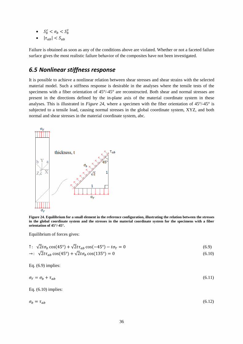
6.5 Nonlinear stiffness response
It is possible to achieve a nonlinear relation between shear stresses and shear strains with the selected
material model. Such a stiffness response is desirable in the analyses where the tensile tests of the
specimens with a fiber orientation of 45 /-45 are reconstructed. Both shear and normal stresses are
present in the directions defined by the in-plane axis of the material coordinate system in these
analyses. This is illustrated in Figure 24, where a specimen with the fiber orientation of 45 /-45 is
subjected to a tensile load, causing normal stresses in the global coordinate system, XYZ, and both
normal and shear stresses in the material coordinate system, abc.
Figure 24. Equilibrium for a small element in the reference configuration, illustrating the relation between the stresses
in the global coordinate system and the stresses in the material coordinate system for the specimens with a fiber
orientation of 45°/-45°.
Equilibrium of forces gives:
√ ( ) √ ( ) (6.9)
√ ( ) √ ( ) (6.10)
Eq. (6.9) implies:
(6.11)
Eq. (6.10) implies:
(6.12)
37
Eq. (6.11) in combination with Eq. (6.12) implies:
(6.13)
Hence, both shear stresses and normal stresses are present in the material coordinate system. In the
reference configuration these stresses are of the same magnitude. The additional input parameters
necessary to obtain the nonlinear stiffness response are presented below.
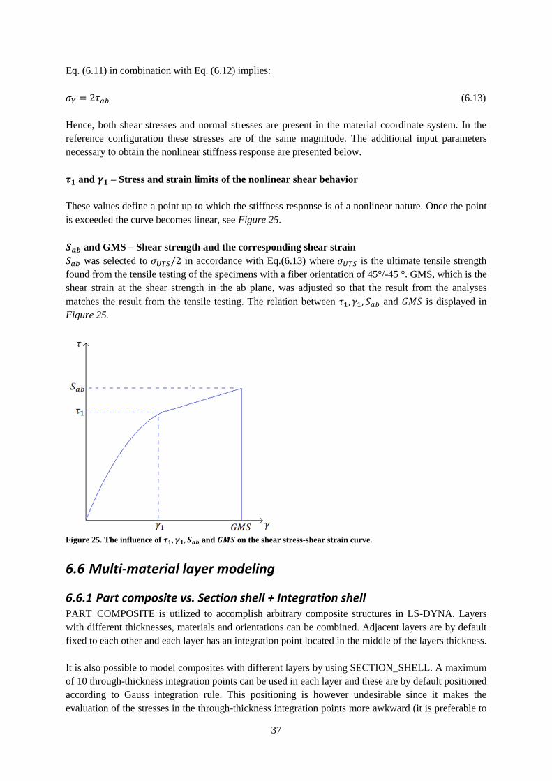
and – Stress and strain limits of the nonlinear shear behavior
These values define a point up to which the stiffness response is of a nonlinear nature. Once the point
is exceeded the curve becomes linear, see Figure 25.
and GMS – Shear strength and the corresponding shear strain
was selected to in accordance with Eq.(6.13) where is the ultimate tensile strength
found from the tensile testing of the specimens with a fiber orientation of 45°/-45 °. GMS, which is the
shear strain at the shear strength in the ab plane, was adjusted so that the result from the analyses
matches the result from the tensile testing. The relation between and is displayed in
Figure 25.
Figure 25. The influence of and on the shear stress-shear strain curve.
6.6 Multi-material layer modeling
6.6.1 Part composite vs. Section shell + Integration shell PART_COMPOSITE is utilized to accomplish arbitrary composite structures in LS-DYNA. Layers
with different thicknesses, materials and orientations can be combined. Adjacent layers are by default
fixed to each other and each layer has an integration point located in the middle of the layers thickness.
It is also possible to model composites with different layers by using SECTION_SHELL. A maximum
of 10 through-thickness integration points can be used in each layer and these are by default positioned
according to Gauss integration rule. This positioning is however undesirable since it makes the
evaluation of the stresses in the through-thickness integration points more awkward (it is preferable to
38
have integration points in the middle of each layer). This can be solved by INTEGRATION_SHELL
which enables user-defined positioning of the through-thickness integration points.
Both approaches have been investigated with the conclusion being that equivalent results are obtained
regardless of the approach used. PART_COMPOSITE was selected since it was perceived as more
user-friendly.
A drawback with through-thickness integration points located in the middle of the layers thickness (as
is the case when modeling with PART_COMPOSITE) is that the tensile and compressive strengths of
the material are not evaluated at the upper and lower surfaces of the composite. Evaluation on the
surface is desirable when bending stresses are present. The influence of this can be reduced by
increasing the number of layers modeled in the composite but this is followed by an increased CPU-
time.
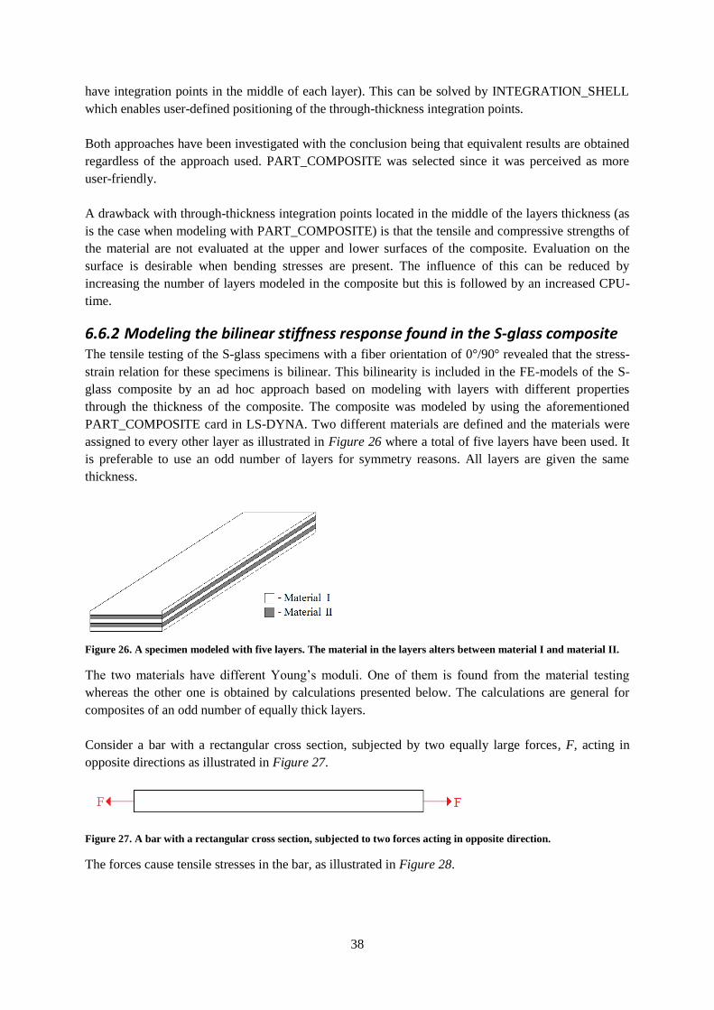
6.6.2 Modeling the bilinear stiffness response found in the S-glass composite The tensile testing of the S-glass specimens with a fiber orientation of 0 /90 revealed that the stress-
strain relation for these specimens is bilinear. This bilinearity is included in the FE-models of the S-
glass composite by an ad hoc approach based on modeling with layers with different properties
through the thickness of the composite. The composite was modeled by using the aforementioned
PART_COMPOSITE card in LS-DYNA. Two different materials are defined and the materials were
assigned to every other layer as illustrated in Figure 26 where a total of five layers have been used. It
is preferable to use an odd number of layers for symmetry reasons. All layers are given the same
thickness.
Figure 26. A specimen modeled with five layers. The material in the layers alters between material I and material II.
The two materials have different Young’s moduli. One of them is found from the material testing
whereas the other one is obtained by calculations presented below. The calculations are general for
composites of an odd number of equally thick layers.
Consider a bar with a rectangular cross section, subjected by two equally large forces, F, acting in
opposite directions as illustrated in Figure 27.
Figure 27. A bar with a rectangular cross section, subjected to two forces acting in opposite direction.
The forces cause tensile stresses in the bar, as illustrated in Figure 28.
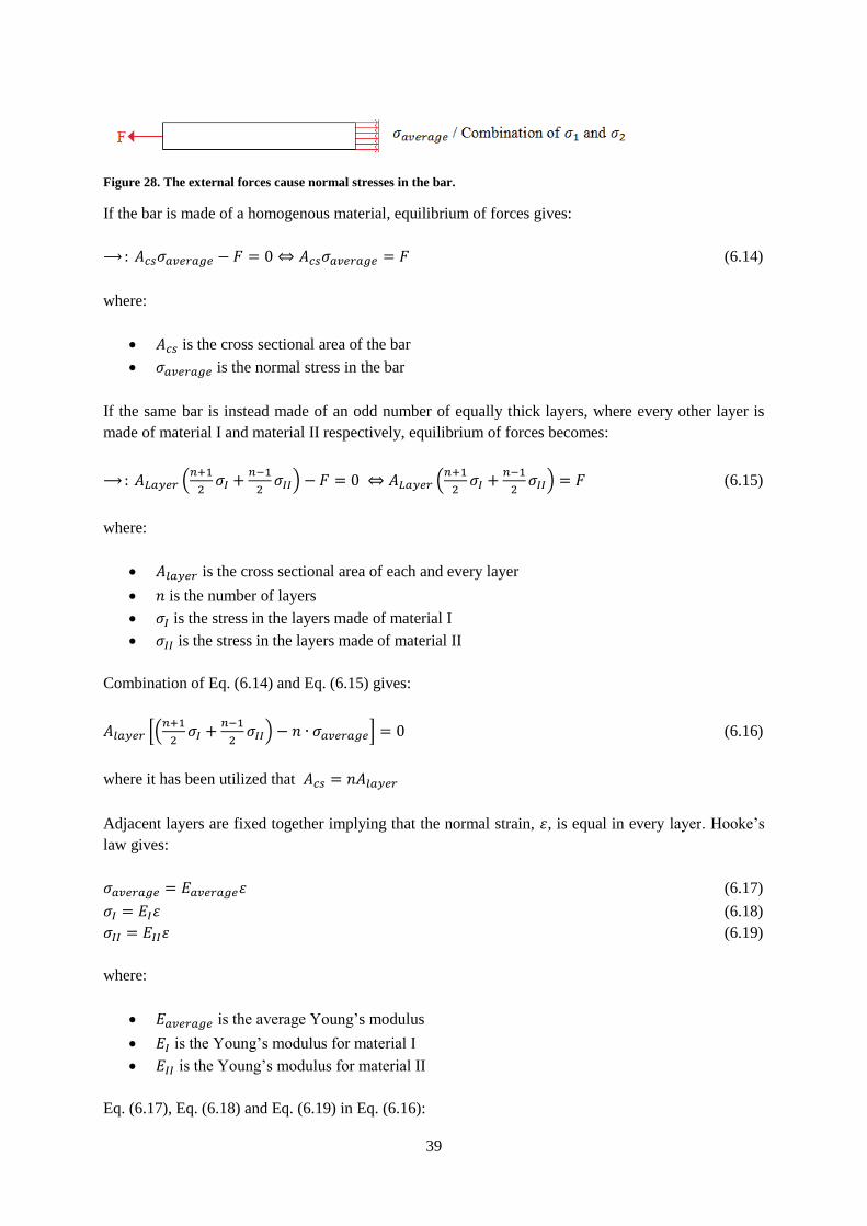
39
Figure 28. The external forces cause normal stresses in the bar.
If the bar is made of a homogenous material, equilibrium of forces gives:
(6.14)
where:
is the cross sectional area of the bar
is the normal stress in the bar
If the same bar is instead made of an odd number of equally thick layers, where every other layer is
made of material I and material II respectively, equilibrium of forces becomes:
(
) (
) (6.15)
where:
is the cross sectional area of each and every layer
is the number of layers
is the stress in the layers made of material I
is the stress in the layers made of material II
Combination of Eq. (6.14) and Eq. (6.15) gives:
[(
) ] (6.16)
where it has been utilized that
Adjacent layers are fixed together implying that the normal strain, , is equal in every layer. Hooke’s
law gives:
(6.17)
(6.18)
(6.19)
where:
is the average Young’s modulus
is the Young’s modulus for material I
is the Young’s modulus for material II
Eq. (6.17), Eq. (6.18) and Eq. (6.19) in Eq. (6.16):
40
(
) (
) (6.20)
where and have been cancelled.
corresponds to the Young’s modulus prior to the transition point found in the right hand side
plot in Figure 8 and corresponds to the linear stress-strain relation found beyond the transition
point in the same plot. Eq. (6.20) enables calculation of . Once the Young’s moduli are known, the
ultimate tensile strengths,
and
of the materials can be determined.
where is the strain at transition point and is equal to in Table 5.
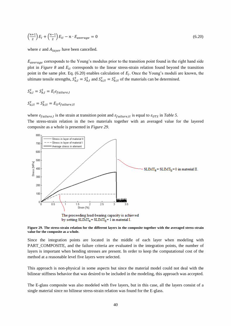
The stress-strain relation in the two materials together with an averaged value for the layered
composite as a whole is presented in Figure 29.
Figure 29. The stress-strain relation for the different layers in the composite together with the averaged stress-strain
value for the composite as a whole.
Since the integration points are located in the middle of each layer when modeling with
PART_COMPOSITE, and the failure criteria are evaluated in the integration points, the number of
layers is important when bending stresses are present. In order to keep the computational cost of the
method at a reasonable level five layers were selected.
This approach is non-physical in some aspects but since the material model could not deal with the
bilinear stiffness behavior that was desired to be included in the modeling, this approach was accepted.
The E-glass composite was also modeled with five layers, but in this case, all the layers consist of a
single material since no bilinear stress-strain relation was found for the E-glass.
41
7 FE modeling of executed tests
7.1 Geometries and boundary conditions
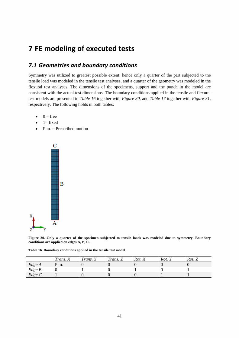
Symmetry was utilized to greatest possible extent; hence only a quarter of the part subjected to the
tensile load was modeled in the tensile test analyses, and a quarter of the geometry was modeled in the
flexural test analyses. The dimensions of the specimens, support and the punch in the model are
consistent with the actual test dimensions. The boundary conditions applied in the tensile and flexural
test models are presented in Table 16 together with Figure 30, and Table 17 together with Figure 31,
respectively. The following holds in both tables:
0 = free
1= fixed
P.m. = Prescribed motion
Figure 30. Only a quarter of the specimen subjected to tensile loads was modeled due to symmetry. Boundary
conditions are applied on edges A, B, C.
Table 16. Boundary conditions applied in the tensile test model.
Trans. X Trans. Y Trans. Z Rot. X Rot. Y Rot. Z
Edge A P.m. 0 0 0 0 0
Edge B 0 1 0 1 0 1
Edge C 1 0 0 0 1 1
42
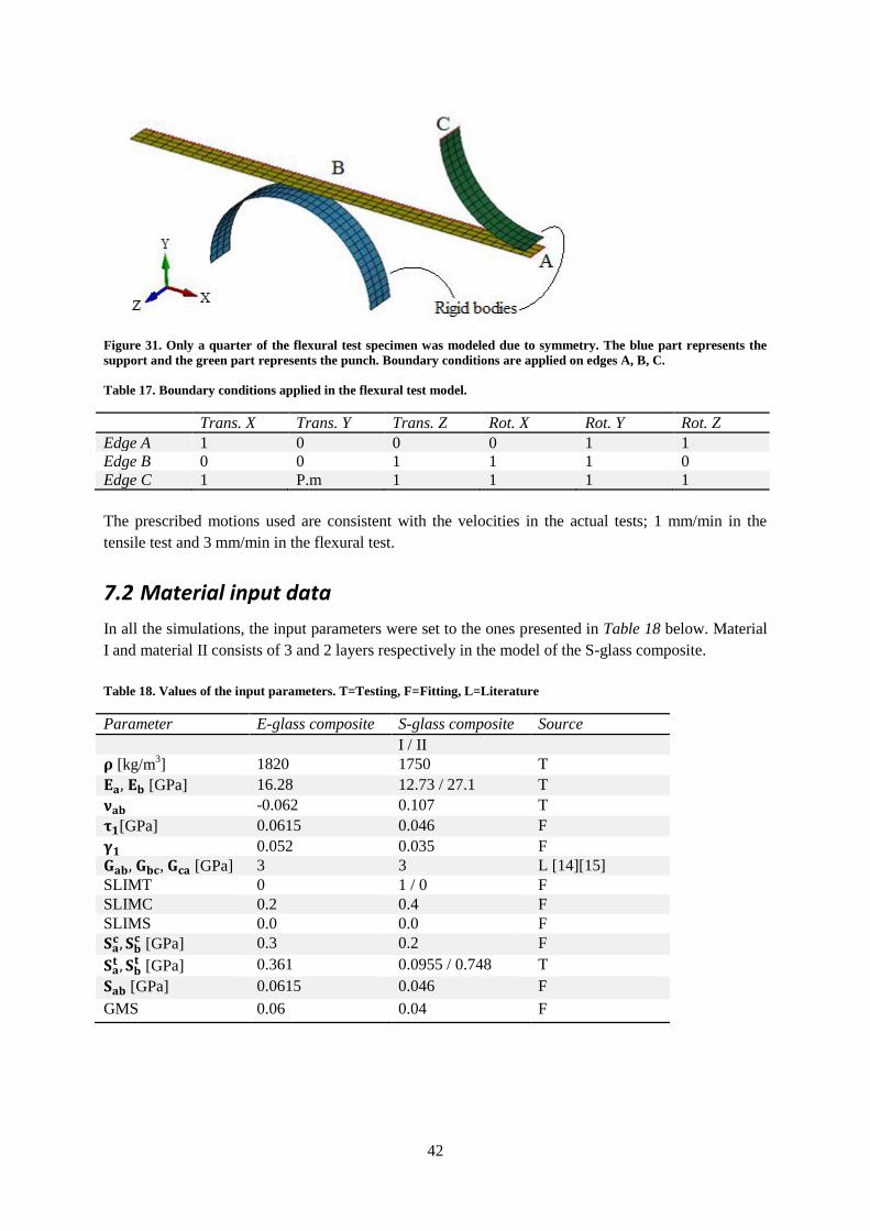
Figure 31. Only a quarter of the flexural test specimen was modeled due to symmetry. The blue part represents the
support and the green part represents the punch. Boundary conditions are applied on edges A, B, C.
Table 17. Boundary conditions applied in the flexural test model.
Trans. X Trans. Y Trans. Z Rot. X Rot. Y Rot. Z
Edge A 1 0 0 0 1 1
Edge B 0 0 1 1 1 0
Edge C 1 P.m 1 1 1 1
The prescribed motions used are consistent with the velocities in the actual tests; 1 mm/min in the
tensile test and 3 mm/min in the flexural test.
7.2 Material input data
In all the simulations, the input parameters were set to the ones presented in Table 18 below. Material
I and material II consists of 3 and 2 layers respectively in the model of the S-glass composite.
Table 18. Values of the input parameters. T=Testing, F=Fitting, L=Literature
Parameter E-glass composite S-glass composite Source
I / II
[kg/m3] 1820 1750 T
[GPa] 16.28 12.73 / 27.1 T
-0.062 0.107 T
[GPa] 0.0615 0.046 F
0.052 0.035 F
, [GPa] 3 3 L [14][15]
SLIMT 0 1 / 0 F
SLIMC 0.2 0.4 F
SLIMS 0.0 0.0 F
[GPa] 0.3 0.2 F
[GPa] 0.361 0.0955 / 0.748 T
[GPa] 0.0615 0.046 F
GMS 0.06 0.04 F
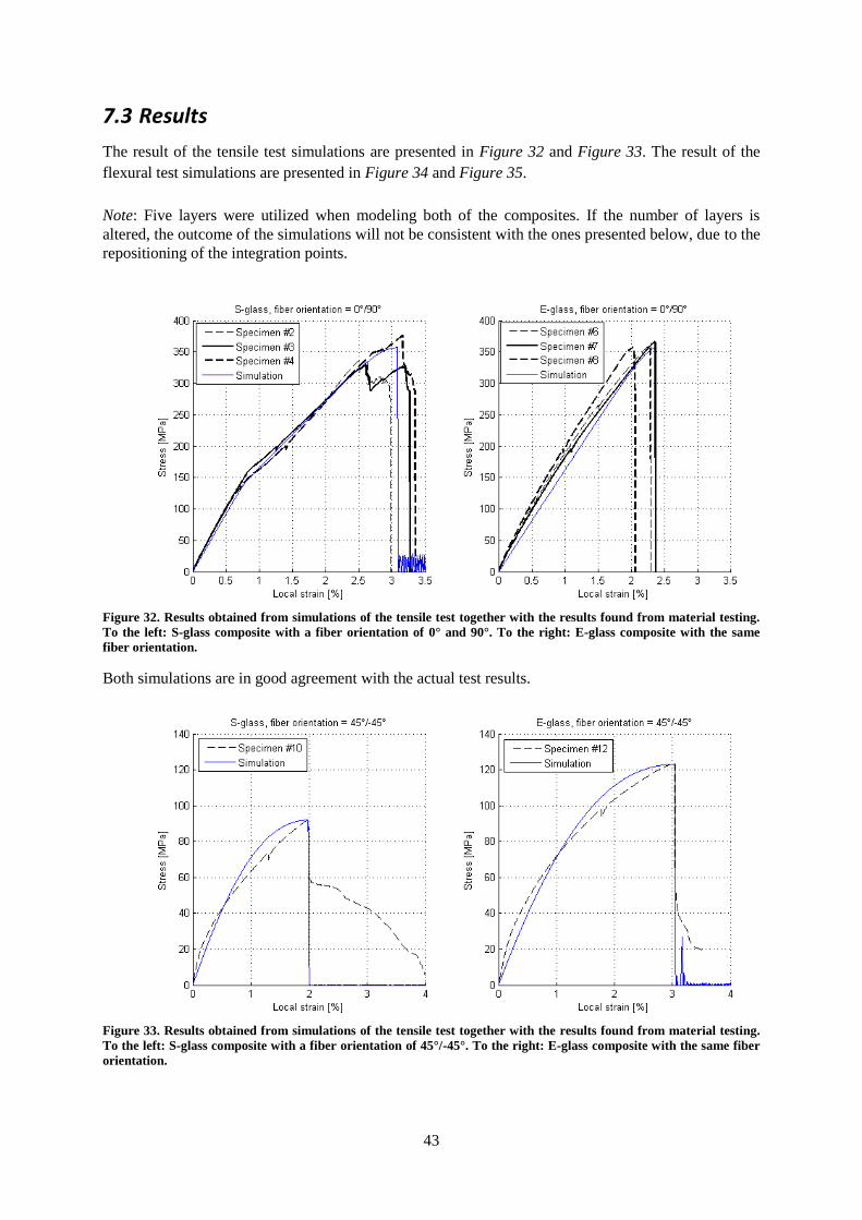
43
7.3 Results
The result of the tensile test simulations are presented in Figure 32 and Figure 33. The result of the
flexural test simulations are presented in Figure 34 and Figure 35.
Note: Five layers were utilized when modeling both of the composites. If the number of layers is
altered, the outcome of the simulations will not be consistent with the ones presented below, due to the
repositioning of the integration points.
Figure 32. Results obtained from simulations of the tensile test together with the results found from material testing.
To the left: S-glass composite with a fiber orientation of 0° and 90°. To the right: E-glass composite with the same
fiber orientation.
Both simulations are in good agreement with the actual test results.
Figure 33. Results obtained from simulations of the tensile test together with the results found from material testing.
To the left: S-glass composite with a fiber orientation of 45°/-45°. To the right: E-glass composite with the same fiber
orientation.
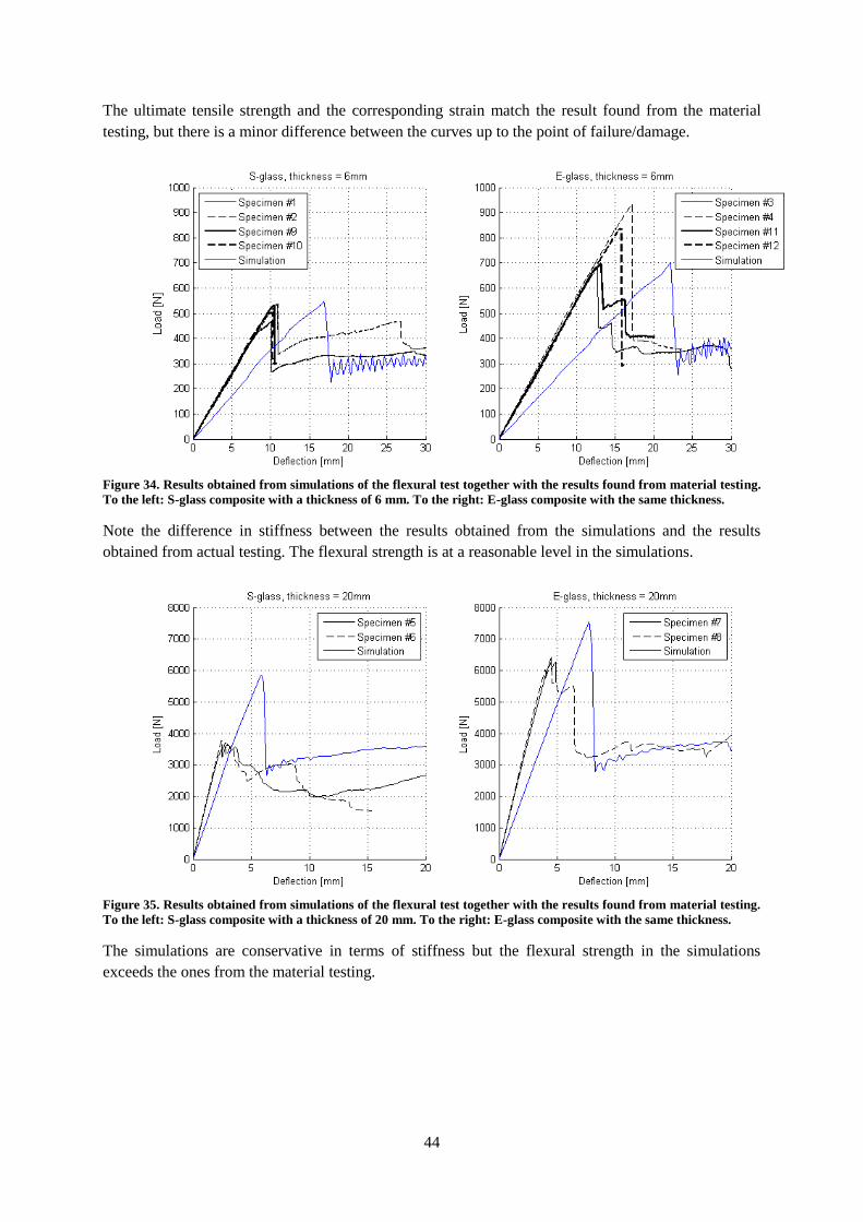
44
The ultimate tensile strength and the corresponding strain match the result found from the material
testing, but there is a minor difference between the curves up to the point of failure/damage.
Figure 34. Results obtained from simulations of the flexural test together with the results found from material testing.
To the left: S-glass composite with a thickness of 6 mm. To the right: E-glass composite with the same thickness.
Note the difference in stiffness between the results obtained from the simulations and the results
obtained from actual testing. The flexural strength is at a reasonable level in the simulations.
Figure 35. Results obtained from simulations of the flexural test together with the results found from material testing.
To the left: S-glass composite with a thickness of 20 mm. To the right: E-glass composite with the same thickness.
The simulations are conservative in terms of stiffness but the flexural strength in the simulations
exceeds the ones from the material testing.
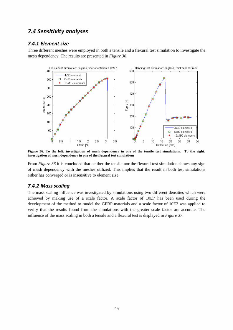
45
7.4 Sensitivity analyses
7.4.1 Element size Three different meshes were employed in both a tensile and a flexural test simulation to investigate the
mesh dependency. The results are presented in Figure 36.
Figure 36. To the left: investigation of mesh dependency in one of the tensile test simulations. To the right:
investigation of mesh dependency in one of the flexural test simulations
From Figure 36 it is concluded that neither the tensile nor the flexural test simulation shows any sign
of mesh dependency with the meshes utilized. This implies that the result in both test simulations
either has converged or is insensitive to element size.
7.4.2 Mass scaling The mass scaling influence was investigated by simulations using two different densities which were
achieved by making use of a scale factor. A scale factor of 10E7 has been used during the
development of the method to model the GFRP-materials and a scale factor of 10E2 was applied to
verify that the results found from the simulations with the greater scale factor are accurate. The
influence of the mass scaling in both a tensile and a flexural test is displayed in Figure 37.
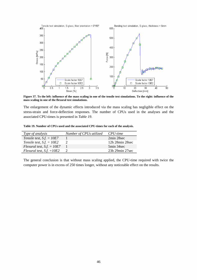
46
Figure 37. To the left: influence of the mass scaling in one of the tensile test simulations. To the right: influence of the
mass scaling in one of the flexural test simulations.
The enlargement of the dynamic effects introduced via the mass scaling has negligible effect on the
stress-strain and force-deflection responses. The number of CPUs used in the analyses and the
associated CPU-times is presented in Table 19.
Table 19. Number of CPUs used and the associated CPU-times for each of the analysis.
Type of analysis Number of CPUs utilized CPU-time
Tensile test, S.f. = 10E7 1 2min 28sec
Tensile test, S.f. = 10E2 2 12h 28min 28sec
Flexural test, S.f. = 10E7 1 5min 34sec
Flexural test, S.f. =10E2 2 23h 29min 27sec
The general conclusion is that without mass scaling applied, the CPU-time required with twice the
computer power is in excess of 250 times longer, without any noticeable effect on the results.
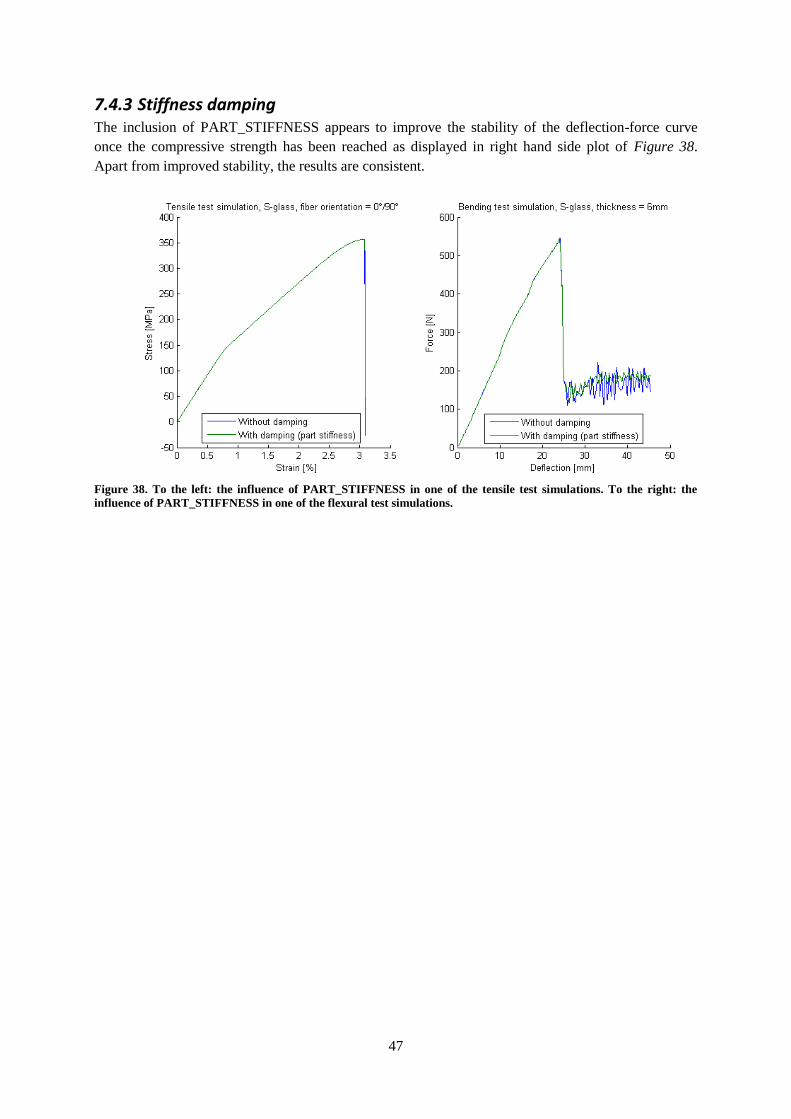
47
7.4.3 Stiffness damping The inclusion of PART_STIFFNESS appears to improve the stability of the deflection-force curve
once the compressive strength has been reached as displayed in right hand side plot of Figure 38.
Apart from improved stability, the results are consistent.
Figure 38. To the left: the influence of PART_STIFFNESS in one of the tensile test simulations. To the right: the
influence of PART_STIFFNESS in one of the flexural test simulations.
48
7.5 Discussion and conclusions
Tensile test analyses, specimens with a fiber orientation of 0 /90 The results from the analyses coincide reasonably well with the results from the material testing for
both the composites and the bilinearity is captured well in the analyses of the S-glass composite.
Tensile test analyses, specimens with a fiber orientation of 45 /-45 The simulations are in good agreement with the actual tests in terms of the ultimate tensile strength
and the corresponding strain.
Even though the curves do not coincide precisely, the result is considered to be acceptable since the
materials ability to absorb energy before failure occurs is approximately the same (the area under the
curves up to failure). Energy absorption is central in the application in which the developed method is
intended to be applied.
The continuous load-bearing capacity exhibited in the actual tests once the material has been damaged
is neglected in the simulations where the damage is treated as a failure instead. The reason for this is
that it is preferable to be somewhat conservative.
Flexural test analyses, specimens with a thickness of 6 mm
The simulation results are not in perfect agreement with the flexural test results. This was expected
since the flexural modulus of elasticity found from the flexural tests was higher than the Young’s
modulus found from the tensile tests, which is the one applied in the simulations. However, the results
are on the conservative side (exaggerated deflections) and the flexural strength is consistent with the
actual flexural strength.
The continuous load-bearing capacity in the simulations is in agreement with the actual tests.
Flexural test analyses, specimens with a thickness of 20 mm
As expected, the results of these analyses are of very poor quality. The stiffness is on the conservative
side but the flexural strength in the analyses exceeds the actual flexural strength. This is presumably
caused by the presence of large out of plane shear stresses in the actual test specimens. A model based
on solid elements could be a better approach to solve this problem.
Conclusions:
The developed method to model the GFRP-materials captures the materials behavior for the
situations investigated, where plane stress can be assumed.
The method is somewhat conservative in terms of bending stiffness, with respect to the actual
tests.
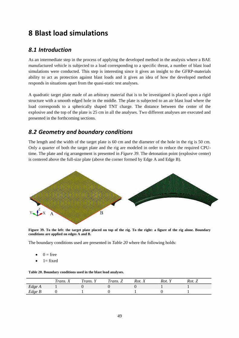
49
8 Blast load simulations
8.1 Introduction
As an intermediate step in the process of applying the developed method in the analysis where a BAE
manufactured vehicle is subjected to a load corresponding to a specific threat, a number of blast load
simulations were conducted. This step is interesting since it gives an insight to the GFRP-materials
ability to act as protection against blast loads and it gives an idea of how the developed method
responds in situations apart from the quasi-static test analyses.
A quadratic target plate made of an arbitrary material that is to be investigated is placed upon a rigid
structure with a smooth edged hole in the middle. The plate is subjected to an air blast load where the
load corresponds to a spherically shaped TNT charge. The distance between the center of the
explosive and the top of the plate is 25 cm in all the analyses. Two different analyses are executed and
presented in the forthcoming sections.
8.2 Geometry and boundary conditions
The length and the width of the target plate is 60 cm and the diameter of the hole in the rig is 50 cm.
Only a quarter of both the target plate and the rig are modeled in order to reduce the required CPU-
time. The plate and rig arrangement is presented in Figure 39. The detonation point (explosive center)
is centered above the full-size plate (above the corner formed by Edge A and Edge B).
Figure 39. To the left: the target plate placed on top of the rig. To the right: a figure of the rig alone. Boundary
conditions are applied on edges A and B.
The boundary conditions used are presented in Table 20 where the following holds:
0 = free
1= fixed
Table 20. Boundary conditions used in the blast load analyses.
Trans. X Trans. Y Trans. Z Rot. X Rot. Y Rot. Z
Edge A 1 0 0 0 1 1
Edge B 0 1 0 1 0 1
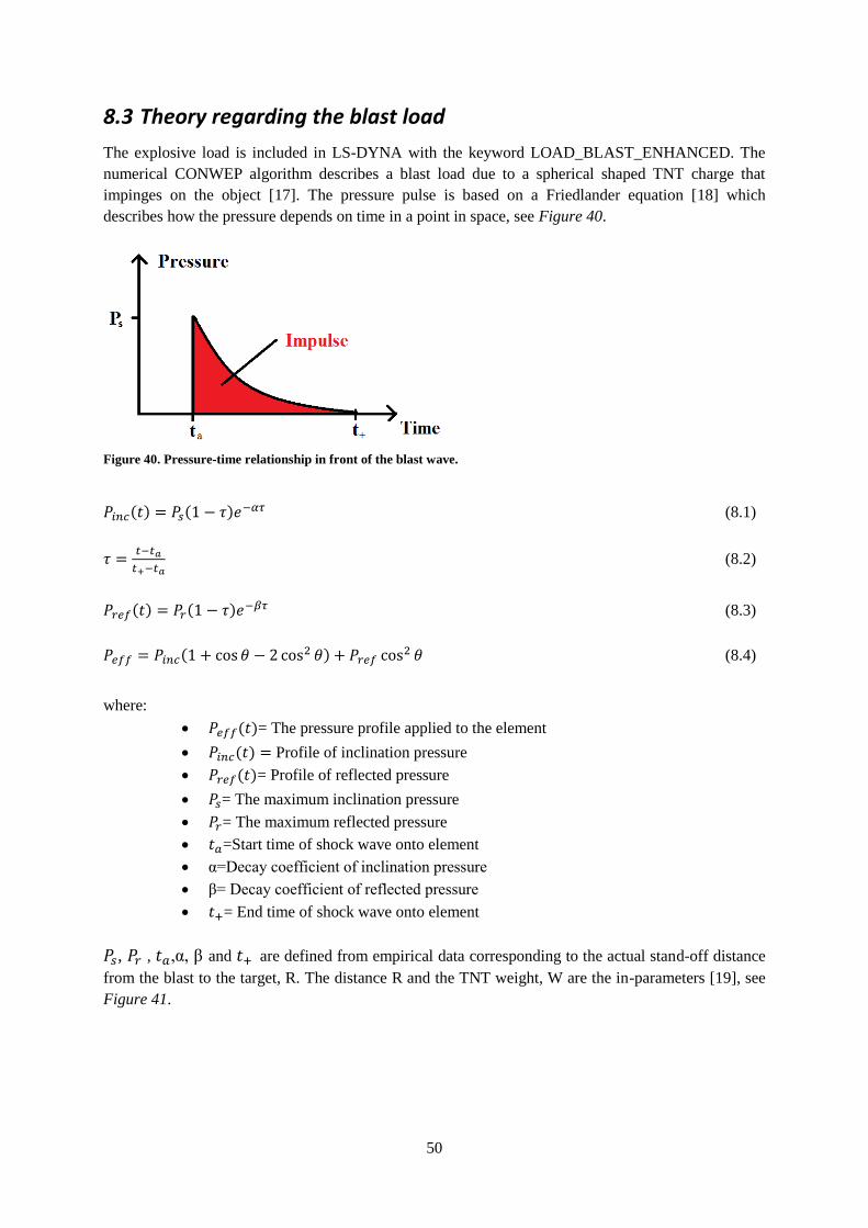
50
8.3 Theory regarding the blast load
The explosive load is included in LS-DYNA with the keyword LOAD_BLAST_ENHANCED. The
numerical CONWEP algorithm describes a blast load due to a spherical shaped TNT charge that
impinges on the object [17]. The pressure pulse is based on a Friedlander equation [18] which
describes how the pressure depends on time in a point in space, see Figure 40.
Figure 40. Pressure-time relationship in front of the blast wave.
( ) ( ) (8.1)
(8.2)
( ) ( ) (8.3)
( )
(8.4)
where:
( )= The pressure profile applied to the element
( ) Profile of inclination pressure
( )= Profile of reflected pressure
= The maximum inclination pressure
= The maximum reflected pressure
=Start time of shock wave onto element
α=Decay coefficient of inclination pressure
β= Decay coefficient of reflected pressure
= End time of shock wave onto element
, , ,α, β and are defined from empirical data corresponding to the actual stand-off distance
from the blast to the target, R. The distance R and the TNT weight, W are the in-parameters [19], see
Figure 41.
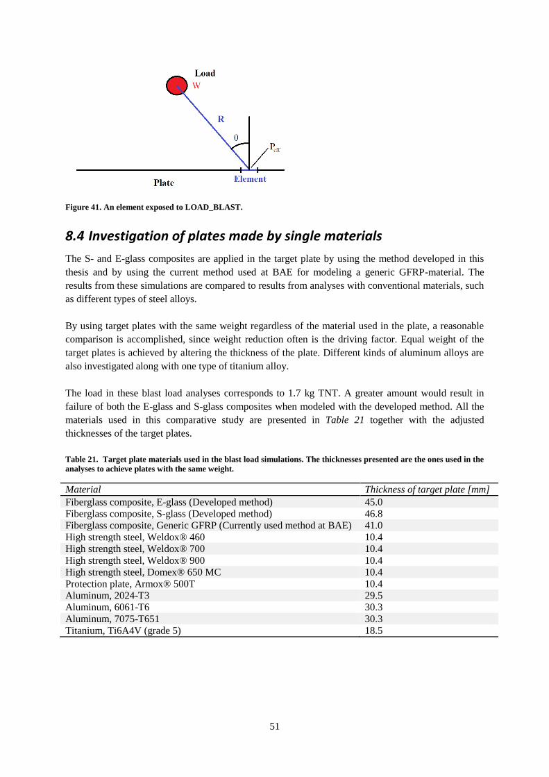
51
Figure 41. An element exposed to LOAD_BLAST.
8.4 Investigation of plates made by single materials
The S- and E-glass composites are applied in the target plate by using the method developed in this
thesis and by using the current method used at BAE for modeling a generic GFRP-material. The
results from these simulations are compared to results from analyses with conventional materials, such
as different types of steel alloys.
By using target plates with the same weight regardless of the material used in the plate, a reasonable
comparison is accomplished, since weight reduction often is the driving factor. Equal weight of the
target plates is achieved by altering the thickness of the plate. Different kinds of aluminum alloys are
also investigated along with one type of titanium alloy.
The load in these blast load analyses corresponds to 1.7 kg TNT. A greater amount would result in
failure of both the E-glass and S-glass composites when modeled with the developed method. All the
materials used in this comparative study are presented in Table 21 together with the adjusted
thicknesses of the target plates.
Table 21. Target plate materials used in the blast load simulations. The thicknesses presented are the ones used in the
analyses to achieve plates with the same weight.
Material Thickness of target plate [mm]
Fiberglass composite, E-glass (Developed method) 45.0
Fiberglass composite, S-glass (Developed method) 46.8
Fiberglass composite, Generic GFRP (Currently used method at BAE) 41.0
High strength steel, Weldox® 460 10.4
High strength steel, Weldox® 700 10.4
High strength steel, Weldox® 900 10.4
High strength steel, Domex® 650 MC 10.4
Protection plate, Armox® 500T 10.4
Aluminum, 2024-T3 29.5
Aluminum, 6061-T6 30.3
Aluminum, 7075-T651 30.3
Titanium, Ti6A4V (grade 5) 18.5
52
8.4.1 Material models The currently used method to model the GFRP-materials at BAE is based on MAT003 –
PLASTIC_KINEMATIC. All the alloys are modeled with MAT098 –
SIMPLIFIED_JOHNSON_COOK. Both material models are intended to be used in the modeling of
isotropic materials with a plastic hardening behavior and both material models have the ability to
include strain rate-effects. Rate-effects are however excluded in these analyses for a fair comparability
of the materials (since rate-effects are not characterized for the GFRP-materials).
The input data applied in the material models are displayed in Table 22, Table 23 and Table 18.
Table 22. The input for the material modeled by MAT003 - Plastic kinematic
MAT003 – PLASTIC_KINEMATIC
Material [kg/m3] [GPa] [-] [MPa] [MPa] BETA [-]
Generic GFRP 2000 10 0.29 100 260 1
where:
is the tangent modulus
BETA = 1 implies an isotropic hardening behavior
Table 23. The input for the materials modeled by MAT098 - Simplified Johnson-Cook.
MAT098 – SIMPLIFIED_JOHNSON_COOK
Material [kg/m3] [GPa] [-] [MPa] [MPa] n [-] Ref.
Titanium
Ti6A4V
(grade 5)
4420 114 0.3416 686 620 0.1 [20]
Weldox®
460 E
7850 210 0.3 499 382 0.458 [21]
Weldox®
700 E
7850 210 0.3 859 329 0.579 [21]
Weldox®
900 E
7850 210 0.3 992 364 0.568 [21]
Aluminum
2024-T3
2780 73.1 0.33 368 683 0.73 [22],[23]
Aluminum
7075-T651
2700 70 0,3 520 477 0.52 [24]
Aluminum
6061-T6
2700 70 0,33 270 154,3 0,2215 [24]
Domex®
650 MC
7850 210 0.33 682 488 0.565 [24]
Armox®
500T
7850 207 0.3 1470 702 0.199 [24]
In the SIMPLIFIED_JOHNSON_COOK model, the flow stress, is defined as:
( )( )
where:
A, B, n and c are material parameters.
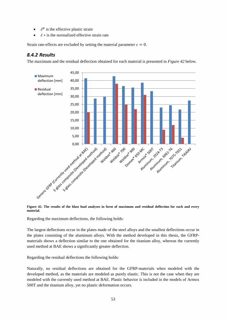
53
is the effective plastic strain
is the normalized effective strain rate
Strain rate-effects are excluded by setting the material parameter .
8.4.2 Results The maximum and the residual deflection obtained for each material is presented in Figure 42 below.
Figure 42. The results of the blast load analyses in form of maximum and residual deflection for each and every
material.
Regarding the maximum deflections, the following holds:
The largest deflections occur in the plates made of the steel alloys and the smallest deflections occur in
the plates consisting of the aluminum alloys. With the method developed in this thesis, the GFRP-
materials shows a deflection similar to the one obtained for the titanium alloy, whereas the currently
used method at BAE shows a significantly greater deflection.
Regarding the residual deflections the following holds:
Naturally, no residual deflections are obtained for the GFRP-materials when modeled with the
developed method, as the materials are modeled as purely elastic. This is not the case when they are
modeled with the currently used method at BAE. Plastic behavior is included in the models of Armox
500T and the titanium alloy, yet no plastic deformation occurs.
0,00
5,00
10,00
15,00
20,00
25,00
30,00
35,00
40,00
45,00Maximumdeflection [mm]
Residualdeflection [mm]
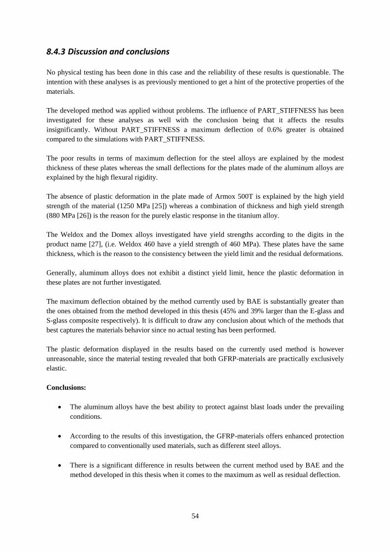
54
8.4.3 Discussion and conclusions
No physical testing has been done in this case and the reliability of these results is questionable. The
intention with these analyses is as previously mentioned to get a hint of the protective properties of the
materials.
The developed method was applied without problems. The influence of PART_STIFFNESS has been
investigated for these analyses as well with the conclusion being that it affects the results
insignificantly. Without PART_STIFFNESS a maximum deflection of 0.6% greater is obtained
compared to the simulations with PART_STIFFNESS.
The poor results in terms of maximum deflection for the steel alloys are explained by the modest
thickness of these plates whereas the small deflections for the plates made of the aluminum alloys are
explained by the high flexural rigidity.
The absence of plastic deformation in the plate made of Armox 500T is explained by the high yield
strength of the material (1250 MPa [25]) whereas a combination of thickness and high yield strength
(880 MPa [26]) is the reason for the purely elastic response in the titanium alloy.
The Weldox and the Domex alloys investigated have yield strengths according to the digits in the
product name [27], (i.e. Weldox 460 have a yield strength of 460 MPa). These plates have the same
thickness, which is the reason to the consistency between the yield limit and the residual deformations.
Generally, aluminum alloys does not exhibit a distinct yield limit, hence the plastic deformation in
these plates are not further investigated.
The maximum deflection obtained by the method currently used by BAE is substantially greater than
the ones obtained from the method developed in this thesis (45% and 39% larger than the E-glass and
S-glass composite respectively). It is difficult to draw any conclusion about which of the methods that
best captures the materials behavior since no actual testing has been performed.
The plastic deformation displayed in the results based on the currently used method is however
unreasonable, since the material testing revealed that both GFRP-materials are practically exclusively
elastic.
Conclusions:
The aluminum alloys have the best ability to protect against blast loads under the prevailing
conditions.
According to the results of this investigation, the GFRP-materials offers enhanced protection
compared to conventionally used materials, such as different steel alloys.
There is a significant difference in results between the current method used by BAE and the
method developed in this thesis when it comes to the maximum as well as residual deflection.
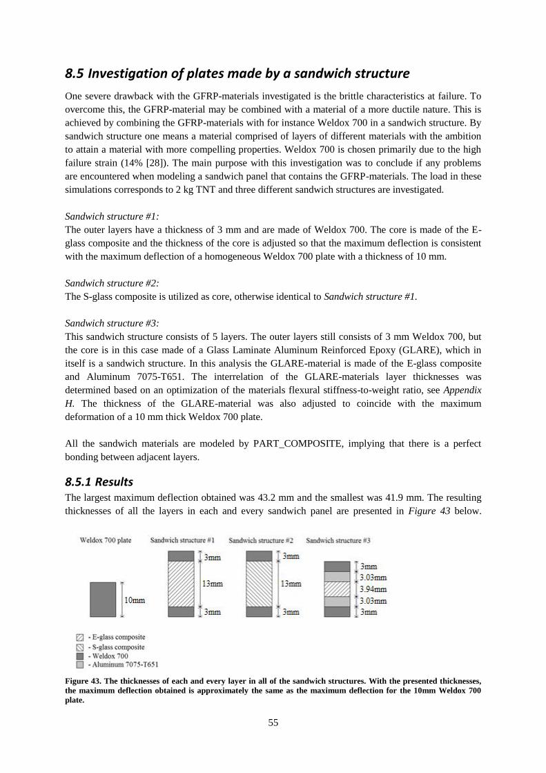
55
8.5 Investigation of plates made by a sandwich structure
One severe drawback with the GFRP-materials investigated is the brittle characteristics at failure. To
overcome this, the GFRP-material may be combined with a material of a more ductile nature. This is
achieved by combining the GFRP-materials with for instance Weldox 700 in a sandwich structure. By
sandwich structure one means a material comprised of layers of different materials with the ambition
to attain a material with more compelling properties. Weldox 700 is chosen primarily due to the high
failure strain (14% [28]). The main purpose with this investigation was to conclude if any problems
are encountered when modeling a sandwich panel that contains the GFRP-materials. The load in these
simulations corresponds to 2 kg TNT and three different sandwich structures are investigated.
Sandwich structure #1:
The outer layers have a thickness of 3 mm and are made of Weldox 700. The core is made of the E-
glass composite and the thickness of the core is adjusted so that the maximum deflection is consistent
with the maximum deflection of a homogeneous Weldox 700 plate with a thickness of 10 mm.
Sandwich structure #2:
The S-glass composite is utilized as core, otherwise identical to Sandwich structure #1.
Sandwich structure #3:
This sandwich structure consists of 5 layers. The outer layers still consists of 3 mm Weldox 700, but
the core is in this case made of a Glass Laminate Aluminum Reinforced Epoxy (GLARE), which in
itself is a sandwich structure. In this analysis the GLARE-material is made of the E-glass composite
and Aluminum 7075-T651. The interrelation of the GLARE-materials layer thicknesses was
determined based on an optimization of the materials flexural stiffness-to-weight ratio, see Appendix
H. The thickness of the GLARE-material was also adjusted to coincide with the maximum
deformation of a 10 mm thick Weldox 700 plate.
All the sandwich materials are modeled by PART_COMPOSITE, implying that there is a perfect
bonding between adjacent layers.
8.5.1 Results The largest maximum deflection obtained was 43.2 mm and the smallest was 41.9 mm. The resulting
thicknesses of all the layers in each and every sandwich panel are presented in Figure 43 below.
Figure 43. The thicknesses of each and every layer in all of the sandwich structures. With the presented thicknesses,
the maximum deflection obtained is approximately the same as the maximum deflection for the 10mm Weldox 700
plate.
56
In Figure 44 the weight of the sandwich structures are related to the weight of the 10 mm Weldox 700
plate.
Figure 44. The weight of the target plates made of sandwich structures in relation to a 10 mm Weldox 700 plate.
The result presented in Figure 44 indicates that a weight reduction of approximately 10% is possible
by utilizing a sandwich structure instead of a homogeneous steel plate, with the same amount of
protection.
There is no remarkable difference between the results obtained for the three sandwich structures.
Sandwich structure #2 is slightly lighter which is due to the lower density of the S-glass composite. It
appears to be unnecessary to introduce a GLARE-material as a core in the sandwich structure.
Notes: These results are only valid for the specified amount of TNT.
8.5.2 Discussion & Conclusions It is possible to include the developed method to model the GFRP-materials in a sandwich structure by
using PART_COMPOSITE.
One drawback was however found with this approach of modeling sandwich structures. This is that
PART_COMPOSITE is based on an assumption of a constant uniform through-thickness strain in the
shell. A sandwich structure modeled with PART_COMPOSITE tends to be too stiff when comprised
of materials with a drastic difference in stiffness [29]. The influence of this assumption has not been
investigated in the executed analyses.
The assumption of a constant uniform through-thickness strain can be accounted for by using
laminated shell theory in LS-DYNA but this is only applicable when sandwich structures are modeled
by SECTION_SHELL with automatically defined through-thickness integration points.
Conclusions:
The developed method can be applied in the modeling of sandwich structures by using
PART_COMPOSITE.
0,82
0,84
0,86
0,88
0,90
0,92
0,94
0,96
0,98
1,00
1,02
Weldox 700plate
Sandwichstructure #1
Sandwichstructure #2
Sandwichstructure #3
Weight in relation to the 10 mmWeldox 700 plate
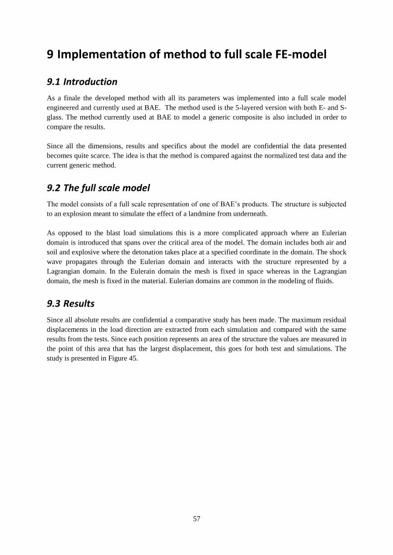
57
9 Implementation of method to full scale FE-model
9.1 Introduction
As a finale the developed method with all its parameters was implemented into a full scale model
engineered and currently used at BAE. The method used is the 5-layered version with both E- and S-
glass. The method currently used at BAE to model a generic composite is also included in order to
compare the results.
Since all the dimensions, results and specifics about the model are confidential the data presented
becomes quite scarce. The idea is that the method is compared against the normalized test data and the
current generic method.
9.2 The full scale model
The model consists of a full scale representation of one of BAE’s products. The structure is subjected
to an explosion meant to simulate the effect of a landmine from underneath.
As opposed to the blast load simulations this is a more complicated approach where an Eulerian
domain is introduced that spans over the critical area of the model. The domain includes both air and
soil and explosive where the detonation takes place at a specified coordinate in the domain. The shock
wave propagates through the Eulerian domain and interacts with the structure represented by a
Lagrangian domain. In the Eulerain domain the mesh is fixed in space whereas in the Lagrangian
domain, the mesh is fixed in the material. Eulerian domains are common in the modeling of fluids.
9.3 Results
Since all absolute results are confidential a comparative study has been made. The maximum residual
displacements in the load direction are extracted from each simulation and compared with the same
results from the tests. Since each position represents an area of the structure the values are measured in
the point of this area that has the largest displacement, this goes for both test and simulations. The
study is presented in Figure 45.
58
Figure 45. Results regarding residual displacements from simulations compared to results from test
9.4 Discussion
One problem that occurred during the simulations with E-glass was high velocities in some nodes in
the composite which lead to error termination. After some investigation it was established that the
problem was due to tensile failure in adjacent elements that lead to zero stiffness in some areas. The
solution to the problem was to introduce a value to the ERODS parameter in the material card. The
ERODS parameter is used to delete elements that exceed a certain value of effective strain. Thanks to
ERODS the diverging nodes would be removed from the simulation and error was avoided. The visual
effect of this was a hole in the structure but the displacement was not affected. The value of ERODS
was chosen to 0.2 since this was the value around which the nodes started to demonstrate divergent
behavior.
Unfortunately the results seem to deviate more from the test results than the current method which
would imply that the new method has lower accuracy, this is hard to tell though from a few numbers.
One must not forget that the introduced method is a tiny part of a complicated model. The deviations
from the current method can be due to interactions between the new method and the rest of the
structure. The error could be due to some other shortcomings that cause excessive deformation
independently from the new method. The important part for the thesis is that the method works and
gives reasonable results.
0%
10%
20%
30%
40%
50%
60%
70%
80%
Position 1 Position 2
Deviation of Residual Displacement compared to test
Generic E-glass S-glass
59
10 Overall conclusions The major conclusions found from this project are presented below.
The S-glass composite generally performs better than the E-glass composite in terms of energy
absorption. Other than that there is no remarkable difference in performance between the two
composites. The S-glass composite did not perform as expected and a bilinearity was found in
the stiffness response obtained from the tensile testing. The reason for this bilinearity has not
been investigated.
A weight reduction of the BAE manufactured vehicles appears to be possible by replacing the
materials in some components with GFRP-materials, without impairing the protection against
some specific threats.
Due to the GFRP-materials brittle characteristics at failure, it is highly recommended to use a
sandwich structure with a more ductile material as outer layers in the protection equipment.
The developed method to model the GFRP-materials in LS-DYNA is more linked to the actual
material compared to the currently used method to model the composites at BAE.
Both the tensile and the flexural test analyses are in good agreement with the results found
from the actual testing when modeled with the developed method. This holds as long as plane
stress can be assumed.
The developed method does not generate better results compared to the current method used at
BAE when implemented in the full scale analyses. It is likely that the results obtained from the
analyses with the developed method would be more similar to the physical results if strain-rate
dependencies are included in the method.
60
11 Further studies
11.1 Changes of the composite material
11.1.1 Composites with another weave structure The plain weave used is not ideal in general structural applications. Composites based on a 4- or 8-
harness weave, quasi isotropic weave (fiber orientation of 0 , 60 and -60 ), or even a quad lay-up of a
unidirectional weave would most likely outperform composites based on a plain weave in the executed
tests. Therefore it seems reasonable to further investigate composites based on the aforementioned
weave structures. This information has been attained from private communications with Owens
Corning [8].
11.1.2 S-glass composites with another type of matrix Even though Owens Corning [8] recommends epoxy as matrix in both the S- and E-glass composites,
it is plausible that the bilinear stiffness response found for the S-glass composite is due to a poor
bonding between the fibers and the matrix. Hence, an investigation of other types of matrices might be
interesting.
11.2 Additional material testing
11.2.1 Shear test The shear modulus was completely sought from literature and a shear test is recommended to
determine the actual shear modulus. Only the in-plane shear modulus is of interest in the developed
method.
11.2.2 Strain rate dependencies A simple upgrade of the material model is possible by switching to MAT158 in which strain-rate
dependencies can be modeled. Naturally this requires additional material testing. Whether or not the
strain-rate is important in GFRP-materials has not been investigated in this work.
61
12 References
[1] – BAE Systems, information provided by the supervisor, 2014
[2] – M. Kinsella, D. Murray, D. Crane, J. Mancinelli, and M. Kranjc, Mechanical properties of
polymeric composites reinforced with high strength glass fibers (2001).
http://www.gagal.agy.com/technical_info/graphics_PDFs/Mech.%20Prop.%20S-
glass%20composites.SAMPE%20Seattle.2001.pdf
[3] – Procedure for the tensile test: ASTM D3039/D3039M - 00 – “Standard Test Method for
Tensile Properties of Polymer Matrix Composite Materials”
[4] – Procedure for the flexural test: ASTM D7264/D7264M - 07 – “Standard Test Method for
Flexural Properties of Polymer Matrix Composite Materials”.
[5] – D. Adams, Tabbing composite test specimens: When and why. Compositesworld (2011)
http://www.compositesworld.com/articles/tabbing-composite-test-specimens-when-and-why
[6] – Owens Corning Corporation, Toledo Ohio USA.
[7] – Nordfarbo AB, Nyland Sverige
[8] – Owens Corning, private communication, 2014
[9] – LS-DYNA Manual Volume II R 7.0
[10] – LS-DYNA Theory Manual March 2006
[11] – LSTC Inc and DYNAmore GmbH. Composite models, LS-DYNA Support (2011).
http://www.dynasupport.com/howtos/material/composite-models
[12] – A. Haufe, K. Schweizerhof, P. DuBois, Properties and Limits: Review of Shell Element
Formulation, Developer Forum, DYNAmore GmbH
http://www.dynamore.de/de/download/papers/2013-ls-dyna-forum/documents/review-of-
shell-element-formulations-in-ls-dyna-properties-limits-advantages-disadvantages
[13] – LSTC Inc. and DYNAmore GmbH. Contact types, LS-DYNA Support (2001).
http://www.dynasupport.com/tutorial/contact-modeling-in-ls-dyna/contact-types
[14] – O. Tomlin, N. Reynolds, Validation of a Thermoplastic Composite Material Model for Low
Carbon Vehicle Applications, WMG, University of Warwick
[15] – D. Samborsky, J. Mandell, P. Agastra, 3-D Static Elastic Constants and Strength Properties
of a Glass/Epoxy Unidirectional Laminate, Dept. of Chemical and Biological Engineering,
Montana State University
62
[16] – K. Schweizerhof, K. Weimar,T Münz, T. Rottner, Crashworthiness Analysis with Enhanced
Composite Material Models in LS-DYNA –Merits and Limits, Inst. For mechanics,
University of Karlsruhe
[17] – G.Randers-Pehrson, K. Bannister, Airblast Loading Model for DYNA2D and DYNA3D,
Army Research Laboratory, 1997
[18] – T. Slavik , A Coupling of Empirical Explosive Blast Loads to ALE Air Domains in LS-
DYNA®, Livermore software technology corporation, Livermore California USA
[19] – J. Chock, Review of Methods for Calculating Pressure Profiles of Explosive Air Blast and its
Sample Applications, Faculty of the Virginia Polytechnic Institute and State University, 1999
[20] – A. Tjernberg, Penetration simulations of titanium plates, Swedish Defense Research
Agency, 2004
[21] – S. Dey, O. Hoppestad T.Børvik, A. Clausen, Constitutive relation and failure criterion for
three steels at high strain rates, Dept. of Structural Engineering, Norwegian University of
Science and Technology.
[22] – G.Kay, Failure Modeling of Titanium 6Al-4V and Aluminum 2024-T3 With the Johnson-
Cook Material Model, Office of Aviation Research, U.S. Dept. of Transportation Federal
Aviation Administration.
[23] – A. Manes, F. Serpellini, M. Pagani, M. Saponara, and M. Giglio, Perforation and
penetration of aluminium target plates by armour piercing bullets. International Journal of
Impact Engineering (2014).
[24] – Material parameters provided by BAE (2014).
[25] – Armox 500T – General product information, SSAB (2014)
http://www.ssab.com/sv/Varumarken/Armox/Produkter1/Armox-500T/
[26] – Aerospace Specification Metals Inc.; Titanium Ti-6Al-4V (Grade 5), Annealed.
http://asm.matweb.com/search/SpecificMaterial.asp?bassnum=MTP641
[27] – General product information WELDOX, HARDOX and ARMOX, SSAB (2005).
http://www.mtlgrp.com/Data/Sites/1/userfiles/pdf/Hardox-Weldox-Armox.pdf
[28] – Weldox 700 – General Product Description, SSAB (2013).
http://www.ssab.com/Global/WELDOX/Datasheets/en/107_WELDOX_700_UK_Da
ta%20Sheet.pdf
[29] – LS-DYNA Manual Volume I R 7.0
[30] – R. D.Cook, D. S. Malkus, M. E. Plesha and R. J. Witt, Concepts and applications of finite
element analysis, 4th ed. University of Wisconsin – Madison (2002).

63
[31] – LSTC Inc. Modeling of composites in LS-DYNA, LS-DYNA Aerospace Working Group
(2013). http://awg.lstc.com/tiki/tiki-download_file.php?fileId=19
[32] – LSTC Inc. and DYNAmore GmbH. Orthotropic materials, LS-DYNA Support (2003).
http://www.dynasupport.com/howtos/material/composite-models
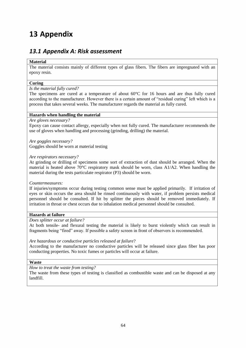
64
13 Appendix
13.1 Appendix A: Risk assessment
Material
The material consists mainly of different types of glass fibers. The fibers are impregnated with an
epoxy resin.
Curing
Is the material fully cured?
The specimens are cured at a temperature of about 60°C for 16 hours and are thus fully cured
according to the manufacturer. However there is a certain amount of “residual curing” left which is a
process that takes several weeks. The manufacturer regards the material as fully cured.
Hazards when handling the material
Are gloves necessary?
Epoxy can cause contact allergy, especially when not fully cured. The manufacturer recommends the
use of gloves when handling and processing (grinding, drilling) the material.
Are goggles necessary?
Goggles should be worn at material testing
Are respirators necessary?
At grinding or drilling of specimens some sort of extraction of dust should be arranged. When the
material is heated above 70°C respiratory mask should be worn, class A1/A2. When handling the
material during the tests particulate respirator (P3) should be worn.
Countermeasures:
If injuries/symptoms occur during testing common sense must be applied primarily. If irritation of
eyes or skin occurs the area should be rinsed continuously with water, if problem persists medical
personnel should be consulted. If hit by splitter the pieces should be removed immediately. If
irritation in throat or chest occurs due to inhalation medical personnel should be consulted.
Hazards at failure
Does splitter occur at failure?
At both tensile- and flexural testing the material is likely to burst violently which can result in
fragments being “fired” away. If possible a safety screen in front of observers is recommended.
Are hazardous or conductive particles released at failure?
According to the manufacturer no conductive particles will be released since glass fiber has poor
conducting properties. No toxic fumes or particles will occur at failure.
Waste
How to treat the waste from testing?
The waste from these types of testing is classified as combustible waste and can be disposed at any
landfill.
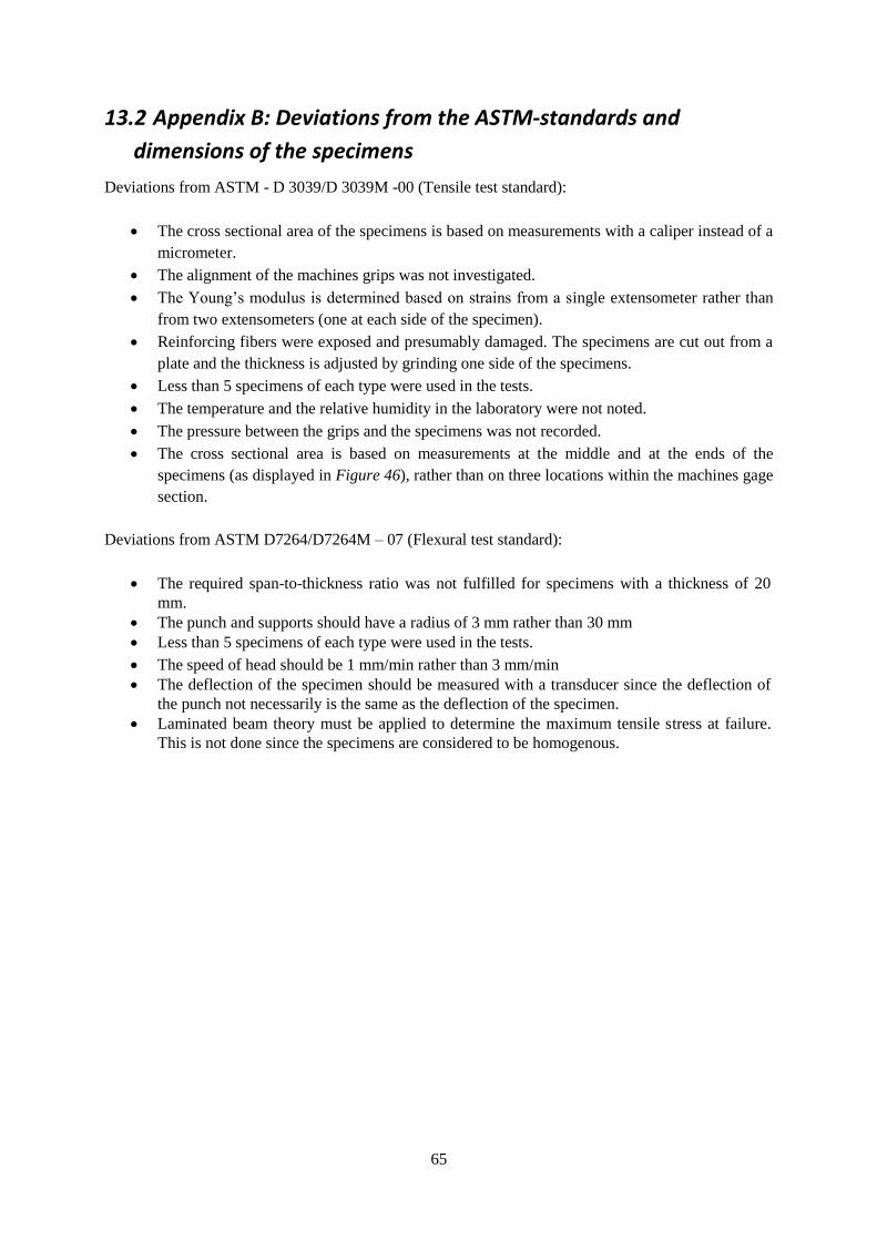
65
13.2 Appendix B: Deviations from the ASTM-standards and
dimensions of the specimens
Deviations from ASTM - D 3039/D 3039M -00 (Tensile test standard):
The cross sectional area of the specimens is based on measurements with a caliper instead of a
micrometer.
The alignment of the machines grips was not investigated.
The Young’s modulus is determined based on strains from a single extensometer rather than
from two extensometers (one at each side of the specimen).
Reinforcing fibers were exposed and presumably damaged. The specimens are cut out from a
plate and the thickness is adjusted by grinding one side of the specimens.
Less than 5 specimens of each type were used in the tests.
The temperature and the relative humidity in the laboratory were not noted.
The pressure between the grips and the specimens was not recorded.
The cross sectional area is based on measurements at the middle and at the ends of the
specimens (as displayed in Figure 46), rather than on three locations within the machines gage
section.
Deviations from ASTM D7264/D7264M – 07 (Flexural test standard):
The required span-to-thickness ratio was not fulfilled for specimens with a thickness of 20
mm.
The punch and supports should have a radius of 3 mm rather than 30 mm
Less than 5 specimens of each type were used in the tests.
The speed of head should be 1 mm/min rather than 3 mm/min
The deflection of the specimen should be measured with a transducer since the deflection of
the punch not necessarily is the same as the deflection of the specimen.
Laminated beam theory must be applied to determine the maximum tensile stress at failure.
This is not done since the specimens are considered to be homogenous.
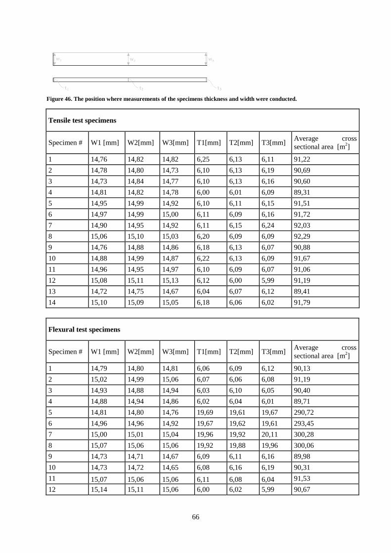
66
Figure 46. The position where measurements of the specimens thickness and width were conducted.
Tensile test specimens
Specimen # W1 [mm] W2[mm] W3[mm] T1[mm] T2[mm] T3[mm] Average cross
sectional area [m2]
1 14,76 14,82 14,82 6,25 6,13 6,11 91,22
2 14,78 14,80 14,73 6,10 6,13 6,19 90,69
3 14,73 14,84 14,77 6,10 6,13 6,16 90,60
4 14,81 14,82 14,78 6,00 6,01 6,09 89,31
5 14,95 14,99 14,92 6,10 6,11 6,15 91,51
6 14,97 14,99 15,00 6,11 6,09 6,16 91,72
7 14,90 14,95 14,92 6,11 6,15 6,24 92,03
8 15,06 15,10 15,03 6,20 6,09 6,09 92,29
9 14,76 14,88 14,86 6,18 6,13 6,07 90,88
10 14,88 14,99 14,87 6,22 6,13 6,09 91,67
11 14,96 14,95 14,97 6,10 6,09 6,07 91,06
12 15,08 15,11 15,13 6,12 6,00 5,99 91,19
13 14,72 14,75 14,67 6,04 6,07 6,12 89,41
14 15,10 15,09 15,05 6,18 6,06 6,02 91,79
Flexural test specimens
Specimen # W1 [mm] W2[mm] W3[mm] T1[mm] T2[mm] T3[mm] Average cross
sectional area [m2]
1 14,79 14,80 14,81 6,06 6,09 6,12 90,13
2 15,02 14,99 15,06 6,07 6,06 6,08 91,19
3 14,93 14,88 14,94 6,03 6,10 6,05 90,40
4 14,88 14,94 14,86 6,02 6,04 6,01 89,71
5 14,81 14,80 14,76 19,69 19,61 19,67 290,72
6 14,96 14,96 14,92 19,67 19,62 19,61 293,45
7 15,00 15,01 15,04 19,96 19,92 20,11 300,28
8 15,07 15,06 15,06 19,92 19,88 19,96 300,06
9 14,73 14,71 14,67 6,09 6,11 6,16 89,98
10 14,73 14,72 14,65 6,08 6,16 6,19 90,31
11 15,07 15,06 15,06 6,11 6,08 6,04 91,53
12 15,14 15,11 15,06 6,00 6,02 5,99 90,67
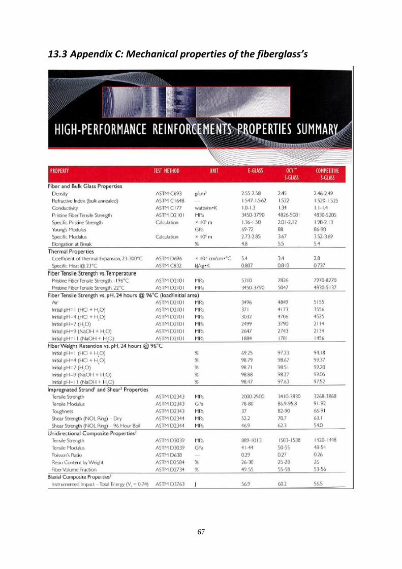
67
13.3 Appendix C: Mechanical properties of the fiberglass’s
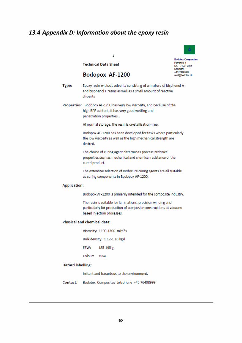
68
13.4 Appendix D: Information about the epoxy resin
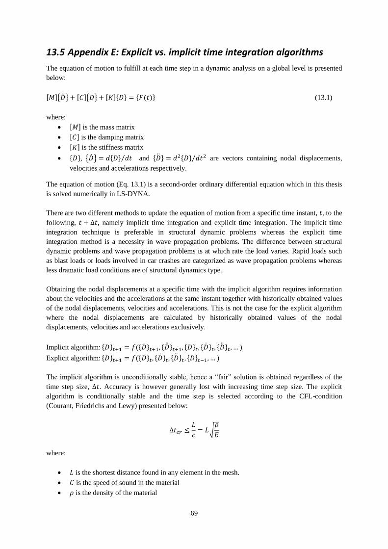
69
13.5 Appendix E: Explicit vs. implicit time integration algorithms
The equation of motion to fulfill at each time step in a dynamic analysis on a global level is presented
below:
[ ]{ } [ ]{ } [ ]{ } { ( )} (13.1)
where:
[ ] is the mass matrix
[ ] is the damping matrix
[ ] is the stiffness matrix
{ }, { } { } ⁄ and { } { } ⁄ are vectors containing nodal displacements,
velocities and accelerations respectively.
The equation of motion (Eq. 13.1) is a second-order ordinary differential equation which in this thesis
is solved numerically in LS-DYNA.
There are two different methods to update the equation of motion from a specific time instant, , to the
following, , namely implicit time integration and explicit time integration. The implicit time
integration technique is preferable in structural dynamic problems whereas the explicit time
integration method is a necessity in wave propagation problems. The difference between structural
dynamic problems and wave propagation problems is at which rate the load varies. Rapid loads such
as blast loads or loads involved in car crashes are categorized as wave propagation problems whereas
less dramatic load conditions are of structural dynamics type.
Obtaining the nodal displacements at a specific time with the implicit algorithm requires information
about the velocities and the accelerations at the same instant together with historically obtained values
of the nodal displacements, velocities and accelerations. This is not the case for the explicit algorithm
where the nodal displacements are calculated by historically obtained values of the nodal
displacements, velocities and accelerations exclusively.
Implicit algorithm: { } ({ } { } { } { } { } )
Explicit algorithm: { } ({ } { } { } { } )
The implicit algorithm is unconditionally stable, hence a “fair” solution is obtained regardless of the
time step size, . Accuracy is however generally lost with increasing time step size. The explicit
algorithm is conditionally stable and the time step is selected according to the CFL-condition
(Courant, Friedrichs and Lewy) presented below:
√
where:
is the shortest distance found in any element in the mesh.
is the speed of sound in the material
is the density of the material

70
is the Young’s modulus of the material
The interpretation of the CFL-condition is that no “information” can travel from one element border to
the adjacent border during one time step. The critical time step size required in the explicit algorithm
is generally significantly smaller than the time step size used in the implicit algorithm. [30]
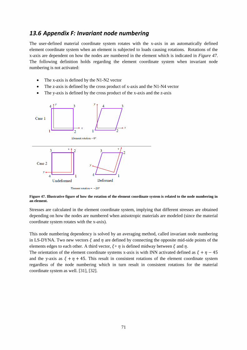
71
13.6 Appendix F: Invariant node numbering
The user-defined material coordinate system rotates with the x-axis in an automatically defined
element coordinate system when an element is subjected to loads causing rotations. Rotations of the
x-axis are dependent on how the nodes are numbered in the element which is indicated in Figure 47.
The following definition holds regarding the element coordinate system when invariant node
numbering is not activated:
The x-axis is defined by the N1-N2 vector
The z-axis is defined by the cross product of x-axis and the N1-N4 vector
The y-axis is defined by the cross product of the x-axis and the z-axis
Figure 47. Illustrative figure of how the rotation of the element coordinate system is related to the node numbering in
an element.
Stresses are calculated in the element coordinate system, implying that different stresses are obtained
depending on how the nodes are numbered when anisotropic materials are modeled (since the material
coordinate system rotates with the x-axis).
This node numbering dependency is solved by an averaging method, called invariant node numbering
in LS-DYNA. Two new vectors and are defined by connecting the opposite mid-side points of the
elements edges to each other. A third vector, + is defined midway between and .
The orientation of the element coordinate systems x-axis is with INN activated defined as
and the y-axis as . This result in consistent rotations of the element coordinate system
regardless of the node numbering which in turn result in consistent rotations for the material
coordinate system as well. [31], [32].
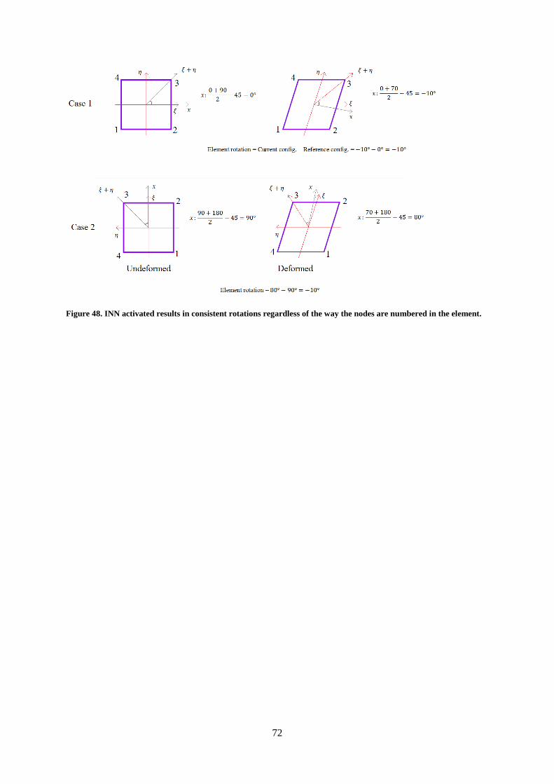
72
Figure 48. INN activated results in consistent rotations regardless of the way the nodes are numbered in the element.
73
13.7 Appendix G: PART_STIFFNESS
PART_STIFFNESS is included to damp high-frequency noise in the analyses. PART_STIFFNESS is
a type of Rayleigh damping, which is a frequency-dependent damping, defining the damping matrix
as:
where:
= Damping matrix
= Mass proportional damping constant
= Mass matrix
= Stiffness proportional damping constant
= Stiffness matrix
In PART_STIFFNESS, is considered to be zero, implying that the damping is based solely on the
stiffness matrix. It is difficult to define a good value of and in LS-DYNA, the coefficient COEF is
used instead. COEF is defined such that a value of 0.10 approximately corresponds to 10% damping in
the high frequency domain. No further explanation is given in the LS-DYNA Theory manual [10].
Damping dissipates energy from the system; hence a careful evaluation of the results is necessary
when nonphysical damping is introduced to the system [30]. In this study, the results of the analyses
with PART_STIFFNESS applied have been compared to the results without any damping.
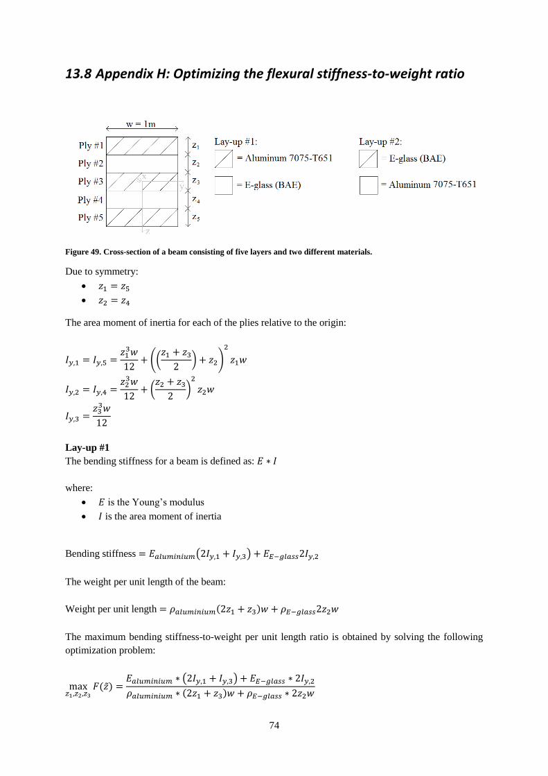
74
13.8 Appendix H: Optimizing the flexural stiffness-to-weight ratio
Figure 49. Cross-section of a beam consisting of five layers and two different materials.
Due to symmetry:
The area moment of inertia for each of the plies relative to the origin:
(( ) )
( )
Lay-up #1
The bending stiffness for a beam is defined as:
where:
is the Young’s modulus
is the area moment of inertia
Bending stiffness ( )
The weight per unit length of the beam:
Weight per unit length ( )
The maximum bending stiffness-to-weight per unit length ratio is obtained by solving the following
optimization problem:
( ) ( )
( )
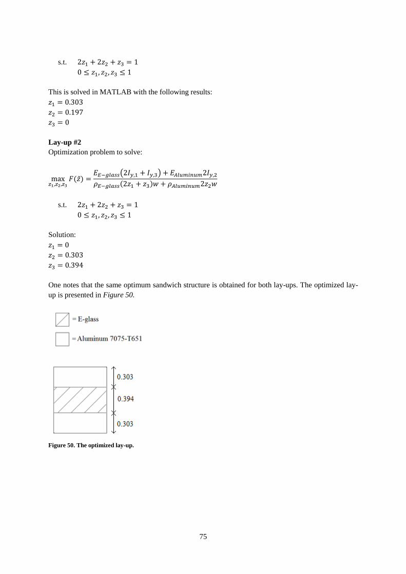
75
s.t.
This is solved in MATLAB with the following results:
Lay-up #2
Optimization problem to solve:
( ) ( )
( )
s.t.
Solution:
One notes that the same optimum sandwich structure is obtained for both lay-ups. The optimized lay-
up is presented in Figure 50.
Figure 50. The optimized lay-up.


![Fiberglass-Epoxy Basics Training Guide[1]](https://img.pdfslide.us/doc/110x75/577cc4b71a28aba7119a3256/fiberglass-epoxy-basics-training-guide1.jpg)