PROCEEDINGS, 43rd Workshop on Geothermal Reservoir Engineering

Stanford University, Stanford, California, February 12-14, 2018

SGP-TR-213

1

Modeling of Coupled Flow, Heat and Mechanical Well Integrity during Variable Geothermal

Production

Jonny Rutqvist, Lehua Pan, Mengsu Hu, Quanlin Zhou, Patrick Dobson

Lawrence Berkeley National Laboratory, Berkeley, California, 94720, U.S.A.

e-mail: jrutqvist@lbl.gov

Keywords: Modeling, well integrity, thermal expansion, variable production, thermal pressurization

ABSTRACT

We investigate the effects of steady and variable geothermal production on mechanical well integrity issues using coupled modeling of

flow, heat and mechanical responses in the well assembly. The coupled process modeling is based on linking the T2Well reservoir-

wellbore simulator with the FLAC3D geomechanical simulator and a detailed discretization of the well assembly, including casing,

cement, wellbore, host rock, and their interfaces. We tested the applicability of this model by conducting a series of simulations of

generic steam-dominant and liquid-dominant systems of both steady and variable geothermal production. The modeling shows that the

highest thermal perturbation, ∆T, occurred in the case of a steam-dominant system in the shallow formations beneath the ground surface

near the production well. In this zone, the temperature increases quickly with production, and decays quickly when the production rate

is reduced during variable or flexible-mode operation, with the highest cyclic increase and decrease of temperature. Moreover,

temperature increases in the cement behind casing causes pressure increases due to thermal pressurization. These temperature and

pressure changes can cause non-linear mechanical responses that are dependent on the thermal expansion of the different components of

the well assembly and include effects of potential frictional sliding at interfaces and material yielding. In the current analysis, we found

that temperature changes during the initial start-up of production could cause cement failure in the shallowest parts of the well both in

tension and compression. The coupled T2Well-FLAC3D model can be applied to better quantify these effects for safe and sustainable

production, both for base-load and flexible production modes.

1. INTRODUCTION

Temporal reduction in geothermal electric production, known as curtailment, has a long history at geothermal operations such as at The

Geysers geothermal field in California (Goyal, 2001). Currently the increased use of variable renewable energy (primarily wind and

solar) increases the inherent variability and uncertainty in electricity demand and resource availability, and thus there is an increasing

demand for operational flexibility of other renewables such as geothermal energy.

Converting production from (steady) base-load to (variable) flexible production may result in significant changes to the system (good or

bad) related to corrosion and mineral deposition (scaling) in wells, mechanical damage fatigue to well components, or the reservoir. One

of the main challenges and concerns related to conversion from base-load to flexible-mode production is wellbore integrity. Flexible-

mode geothermal production typically includes daily cycles in production that result in extraordinary stress on the wellbore and

reservoir system. The detrimental effect of thermal stresses on casing is well known due to years of experience in steam injection in

heavy oilfields and a geothermal well poses even more complex loading issues. The heating and cooling process leads to expansion and

shrinkage of all materials in all scenarios in the well. Especially the casing is affected by temperature changes as metals provide higher

thermal expansion coefficients than cement. Thermal expansion induces forces in the cement sheath, which might lead to cement

failure. Thus, there is a need to investigate the effects of flexible-mode production on well integrity over the operational life of a

geothermal field to be able to optimize the total production and production flexibility at a reduced risk and cost of well failure.

In this study, funded by the California Energy Commission (CEC) to the Lawrence Berkeley National Laboratory (LBNL), the effects

of variable geothermal production on mechanical well integrity is investigated using coupled modeling of flow, heat and mechanical

responses in the well assembly. The coupled modeling is based on linking LBNL’s T2Well reservoir-wellbore simulator with the

FLAC3D geomechanical simulator and a detailed discretization of the well assembly, including casing, cement, wellbore host rock, and

their interfaces. In the following sections, the T2Well-FLAC3D code is first described, followed by the testing of the applicability of

this modeling approach by conducting a series of simulations of generic liquid-dominant and steam-dominant systems of both steady

and variable geothermal production.

2. T2WELL-FLAC3D

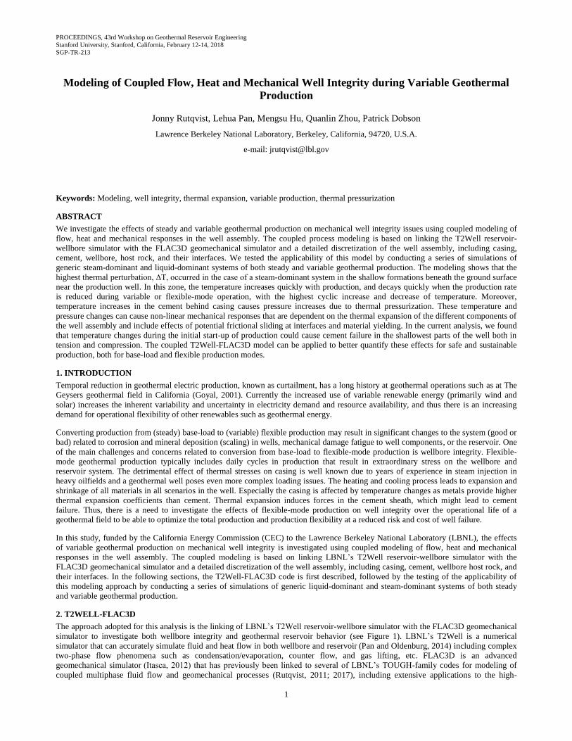
The approach adopted for this analysis is the linking of LBNL’s T2Well reservoir-wellbore simulator with the FLAC3D geomechanical

simulator to investigate both wellbore integrity and geothermal reservoir behavior (see Figure 1). LBNL’s T2Well is a numerical

simulator that can accurately simulate fluid and heat flow in both wellbore and reservoir (Pan and Oldenburg, 2014) including complex

two-phase flow phenomena such as condensation/evaporation, counter flow, and gas lifting, etc. FLAC3D is an advanced

geomechanical simulator (Itasca, 2012) that has previously been linked to several of LBNL’s TOUGH-family codes for modeling of

coupled multiphase fluid flow and geomechanical processes (Rutqvist, 2011; 2017), including extensive applications to the high-

Rutqvist et al.

2

temperature geothermal system at The Geysers geothermal field (Rutqvist et al., 2016, and references therein). Using T2Well linked

with FLAC3D enables accurate modeling of multiphase flow processes within the wellbore and effects of wellbore pressure and

temperature changes on the well (including casing and cement) as well as in surrounding rock.

T2Well and FLAC3D are sequentially coupled, whereby fluid flow variables, such as pore pressure, temperature, and saturation

calculated by T2Well, are transferred to a compatible numerical grid for FLAC3D, which then calculates effective stresses, thermal

strains and associated deformations, returning updated values for porosity, permeability, and capillary strength parameter to T2Well.

The sequential coupling technique was previously adopted for the linking of the TOUGH2 reservoir simulator to FLAC3D

geomechanics simulator (Rutqvist, 2011; 2017). The coupling scheme is based on the fixed stress-split sequential method (Kim et

al., 2011). In this method, the flow problem is solved first (with an explicit evaluation of the volumetric total stress) and the pore

pressure and the temperature are prescribed during the geomechanical calculation, which therefore requires drained mechanical

properties.

One practical advantage with the sequential coupling technique adopted for T2Well-FLAC is the flexibility in the discretization of the

problem domain for the thermal-hydraulic (T2Well) and mechanical (FLAC3D) analysis. In particular, the thermal-hydraulic analysis

will require discretization of the entire well assembly and surrounding rock formations, while the mechanical analysis might be focused

on different sections of the well. For example, the mechanical analysis may be focused on shallow regions of the well where the largest

pressure and temperature changes could occur (Figure 1). Moreover, the flexibility in the mesh discretization enable inclusion of other

critical mechanical components into the mechanical analysis of the well assembly, such as slip interfaces between cement and casing

that may significantly impact the mechanical behavior within the well assembly.

Figure 1: Coupling and interactions between T2Well for reservoir-wellbore multiphase flow and multicomponent transport

modeling and FLAC3D for geomechanical modeling, with application to wellbore integrity analysis by including

reservoir, wellbore and high +∆T zone.

3. THERMAL-HYDRAULIC ANALYSIS OF TEMPERATURE AND PRESSURE RESPONSES

An initial set of simulations were performed with T2Well to model the basic temperature and pressure responses associated with

variable (cyclic) geothermal production. We considered cases of both typical steam-dominant and liquid-dominant geothermal systems.

For the steam-dominant system, actual steady production data from a well at The Geysers geothermal field was used to assure realistic

field conditions in the model. The production data was from Prati 25 (P25), which is one of the production wells associated with the

Northwest Geysers EGS Demonstration Project (Garcia et al., 2016). The Northwest EGS Demonstration site is well characterized and

extensively modeled related to reservoir pressure, temperature and properties and reservoir responses to liquid fluid injection (Garcia et

al., 2016; Rutqvist et al., 2016). The main steam reservoir (so-called normal temperature reservoir at The Geysers) typically has a

reservoir temperature of about 240C and a steam pressure on the order of a few MPa. The model for a typical liquid-dominant

geothermal system was then developed by using the same model of the well assembly and geological layering, but with an assumed

hydrostatic fluid pressure and fully saturated with liquid water.

3.1 Steam-dominant System

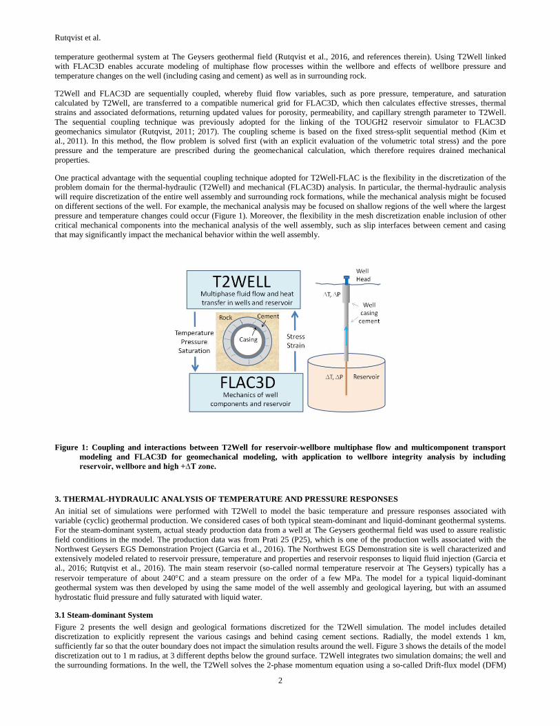
Figure 2 presents the well design and geological formations discretized for the T2Well simulation. The model includes detailed

discretization to explicitly represent the various casings and behind casing cement sections. Radially, the model extends 1 km,

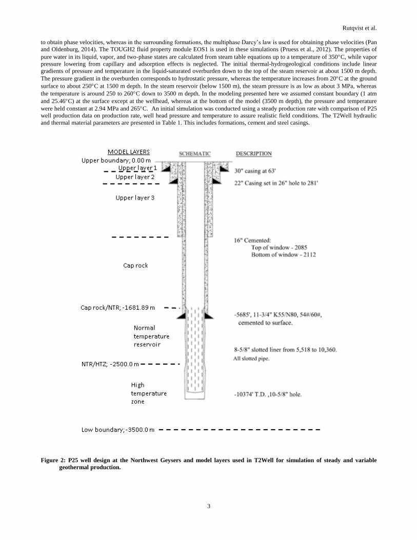
sufficiently far so that the outer boundary does not impact the simulation results around the well. Figure 3 shows the details of the model

discretization out to 1 m radius, at 3 different depths below the ground surface. T2Well integrates two simulation domains; the well and

the surrounding formations. In the well, the T2Well solves the 2-phase momentum equation using a so-called Drift-flux model (DFM)

Rutqvist et al.

3

to obtain phase velocities, whereas in the surrounding formations, the multiphase Darcy’s law is used for obtaining phase velocities (Pan

and Oldenburg, 2014). The TOUGH2 fluid property module EOS1 is used in these simulations (Pruess et al., 2012). The properties of

pure water in its liquid, vapor, and two-phase states are calculated from steam table equations up to a temperature of 350C, while vapor

pressure lowering from capillary and adsorption effects is neglected. The initial thermal-hydrogeological conditions include linear

gradients of pressure and temperature in the liquid-saturated overburden down to the top of the steam reservoir at about 1500 m depth.

The pressure gradient in the overburden corresponds to hydrostatic pressure, whereas the temperature increases from 20C at the ground

surface to about 250C at 1500 m depth. In the steam reservoir (below 1500 m), the steam pressure is as low as about 3 MPa, whereas

the temperature is around 250 to 260C down to 3500 m depth. In the modeling presented here we assumed constant boundary (1 atm

and 25.46C) at the surface except at the wellhead, whereas at the bottom of the model (3500 m depth), the pressure and temperature

were held constant at 2.94 MPa and 265C. An initial simulation was conducted using a steady production rate with comparison of P25

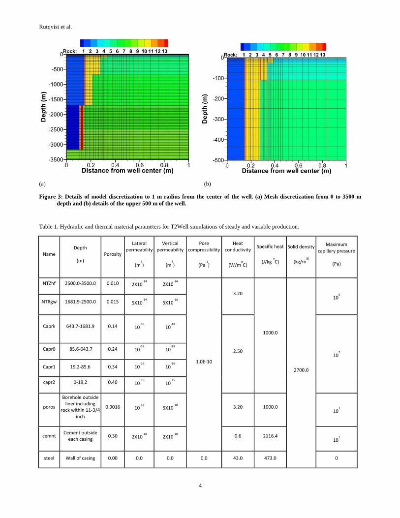
well production data on production rate, well head pressure and temperature to assure realistic field conditions. The T2Well hydraulic

and thermal material parameters are presented in Table 1. This includes formations, cement and steel casings.

Figure 2: P25 well design at the Northwest Geysers and model layers used in T2Well for simulation of steady and variable

geothermal production.

Rutqvist et al.

4

(a) (b)

Figure 3: Details of model discretization to 1 m radius from the center of the well. (a) Mesh discretization from 0 to 3500 m

depth and (b) details of the upper 500 m of the well.

Table 1. Hydraulic and thermal material parameters for T2Well simulations of steady and variable production.

Name Depth

(m) Porosity

Lateral permeability

(m2)

Vertical permeability

(m2)

Pore compressibility

(Pa-1

)

Heat conductivity

(W/moC)

Specific heat

(J/kg oC)

Solid density

(kg/m3)

Maximum capillary pressure

(Pa)

NTZhf 2500.0-3500.0 0.010 2X10-14

2X10-14

1.0E-10

3.20

1000.0

2700.0

105

NTRgw 1681.9-2500.0 0.015 5X10-14

5X10-14

Caprk 643.7-1681.9 0.14 10-18

10-18

2.50 10

7

Capr0 85.6-643.7 0.24 10-18

10-18

Capr1 19.2-85.6 0.34 10-16

10-16

capr2 0-19.2 0.40 10-15

10-15

poros

Borehole outside liner including

rock within 11-3/4 inch

0.9016 10-12

5X10-10

3.20 1000.0 10

3

cemnt Cement outside

each casing 0.30 2X10

-18 2X10

-18 0.6 2116.4

107

steel Wall of casing 0.00 0.0 0.0 0.0 43.0 473.0 0

Rutqvist et al.

5

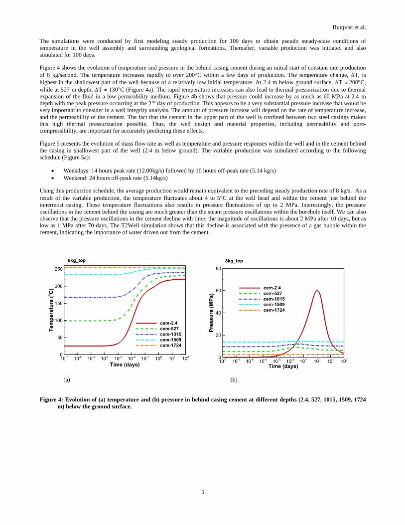
The simulations were conducted by first modeling steady production for 100 days to obtain pseudo steady-state conditions of

temperature in the well assembly and surrounding geological formations. Thereafter, variable production was initiated and also

simulated for 100 days.

Figure 4 shows the evolution of temperature and pressure in the behind casing cement during an initial start of constant rate production

of 8 kg/second. The temperature increases rapidly to over 200C within a few days of production. The temperature change, T, is

highest in the shallowest part of the well because of a relatively low initial temperature. At 2.4 m below ground surface, T 200C,

while at 527 m depth, T 130C (Figure 4a). The rapid temperature increases can also lead to thermal pressurization due to thermal

expansion of the fluid in a low permeability medium. Figure 4b shows that pressure could increase by as much as 60 MPa at 2.4 m

depth with the peak pressure occurring at the 2nd day of production. This appears to be a very substantial pressure increase that would be

very important to consider in a well integrity analysis. The amount of pressure increase will depend on the rate of temperature increase,

and the permeability of the cement. The fact that the cement in the upper part of the well is confined between two steel casings makes

this high thermal pressurization possible. Thus, the well design and material properties, including permeability and pore-

compressibility, are important for accurately predicting these effects.

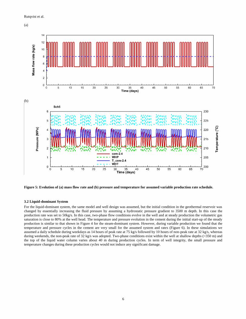
Figure 5 presents the evolution of mass flow rate as well as temperature and pressure responses within the well and in the cement behind

the casing in shallowest part of the well (2.4 m below ground). The variable production was simulated according to the following

schedule (Figure 5a):

Weekdays: 14 hours peak rate (12.00kg/s) followed by 10 hours off-peak rate (5.14 kg/s)

Weekend: 24 hours off-peak rate (5.14kg/s)

Using this production schedule, the average production would remain equivalent to the preceding steady production rate of 8 kg/s. As a

result of the variable production, the temperature fluctuates about 4 to 5C at the well head and within the cement just behind the

innermost casing. These temperature fluctuations also results in pressure fluctuations of up to 2 MPa. Interestingly, the pressure

oscillations in the cement behind the casing are much greater than the steam pressure oscillations within the borehole itself. We can also

observe that the pressure oscillations in the cement decline with time; the magnitude of oscillations is about 2 MPa after 10 days, but as

low as 1 MPa after 70 days. The T2Well simulation shows that this decline is associated with the presence of a gas bubble within the

cement, indicating the importance of water driven out from the cement.

(a) (b)

Figure 4: Evolution of (a) temperature and (b) pressure in behind casing cement at different depths (2.4, 527, 1015, 1509, 1724

m) below the ground surface.

Rutqvist et al.

6

(a)

(b)

Figure 5: Evolution of (a) mass flow rate and (b) pressure and temperature for assumed variable production rate schedule.

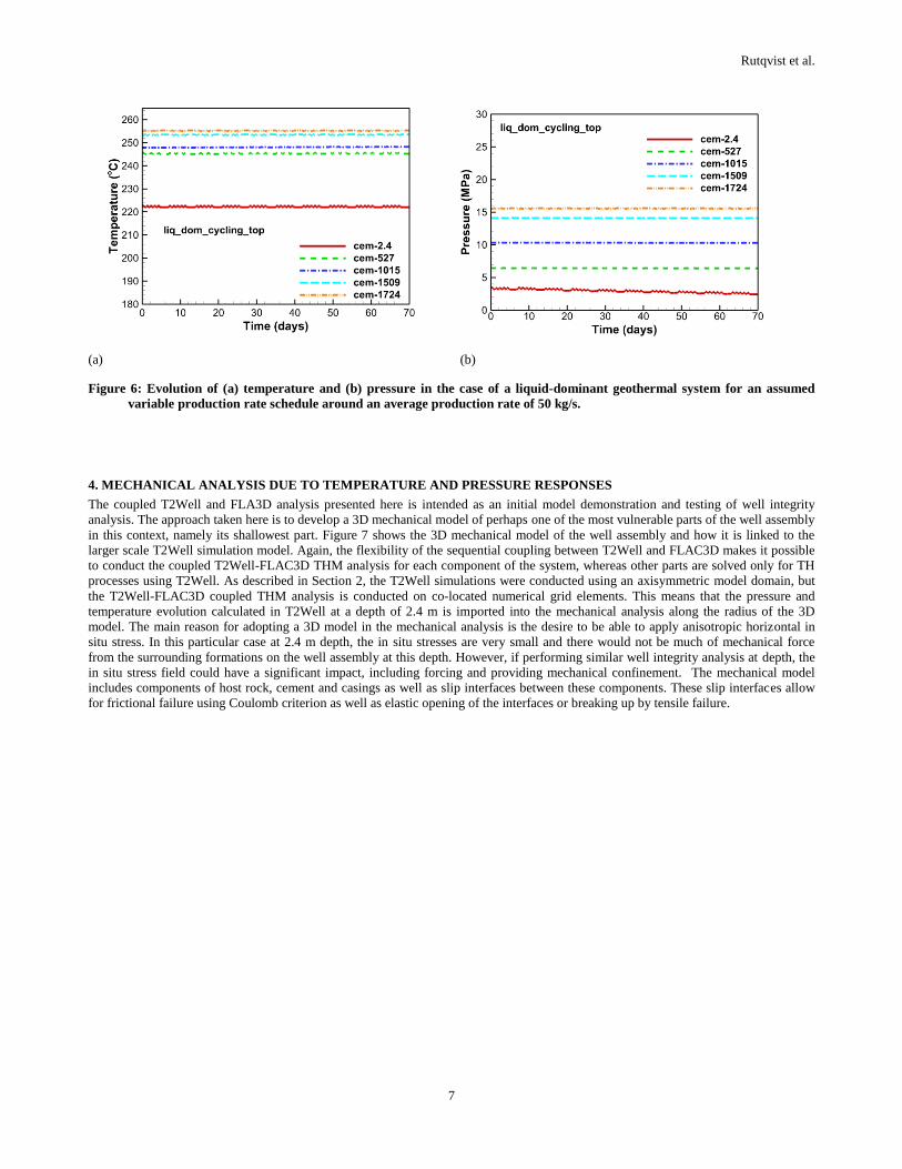
3.2 Liquid-dominant System

For the liquid-dominant system, the same model and well design was assumed, but the initial condition in the geothermal reservoir was

changed by essentially increasing the fluid pressure by assuming a hydrostatic pressure gradient to 3500 m depth. In this case the

production rate was set to 50kg/s. In this case, two-phase flow conditions evolve in the well and at steady production the volumetric gas

saturation is close to 80% at the well head. The temperature and pressure evolution in the cement during the initial start-up of the steady

production is similar to that shown in Figure 4 for the steam-dominant system. However, during variable production we found that the

temperature and pressure cycles in the cement are very small for the assumed system and rates (Figure 6). In these simulations we

assumed a daily schedule during weekdays as 14 hours of peak rate at 75 kg/s followed by 10 hours of non-peak rate at 32 kg/s, whereas

during weekends, the non-peak rate of 32 kg/s was adopted. Two-phase conditions exist within the well at shallow depths (<350 m) and

the top of the liquid water column varies about 40 m during production cycles. In term of well integrity, the small pressure and

temperature changes during these production cycles would not induce any significant damage.

Rutqvist et al.

7

(a) (b)

Figure 6: Evolution of (a) temperature and (b) pressure in the case of a liquid-dominant geothermal system for an assumed

variable production rate schedule around an average production rate of 50 kg/s.

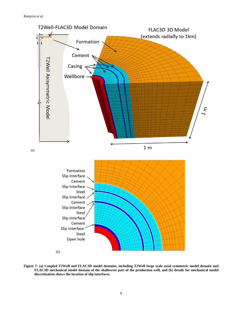
4. MECHANICAL ANALYSIS DUE TO TEMPERATURE AND PRESSURE RESPONSES

The coupled T2Well and FLA3D analysis presented here is intended as an initial model demonstration and testing of well integrity

analysis. The approach taken here is to develop a 3D mechanical model of perhaps one of the most vulnerable parts of the well assembly

in this context, namely its shallowest part. Figure 7 shows the 3D mechanical model of the well assembly and how it is linked to the

larger scale T2Well simulation model. Again, the flexibility of the sequential coupling between T2Well and FLAC3D makes it possible

to conduct the coupled T2Well-FLAC3D THM analysis for each component of the system, whereas other parts are solved only for TH

processes using T2Well. As described in Section 2, the T2Well simulations were conducted using an axisymmetric model domain, but

the T2Well-FLAC3D coupled THM analysis is conducted on co-located numerical grid elements. This means that the pressure and

temperature evolution calculated in T2Well at a depth of 2.4 m is imported into the mechanical analysis along the radius of the 3D

model. The main reason for adopting a 3D model in the mechanical analysis is the desire to be able to apply anisotropic horizontal in

situ stress. In this particular case at 2.4 m depth, the in situ stresses are very small and there would not be much of mechanical force

from the surrounding formations on the well assembly at this depth. However, if performing similar well integrity analysis at depth, the

in situ stress field could have a significant impact, including forcing and providing mechanical confinement. The mechanical model

includes components of host rock, cement and casings as well as slip interfaces between these components. These slip interfaces allow

for frictional failure using Coulomb criterion as well as elastic opening of the interfaces or breaking up by tensile failure.

Rutqvist et al.

8

(a)

(b)

Figure 7: (a) Coupled T2Well and FLAC3D model domains, including T2Well large scale axial symmetric model domain and

FLAC3D mechanical model domain of the shallowest part of the production well, and (b) details for mechanical model

discretization shows the location of slip interfaces.

Rutqvist et al.

9

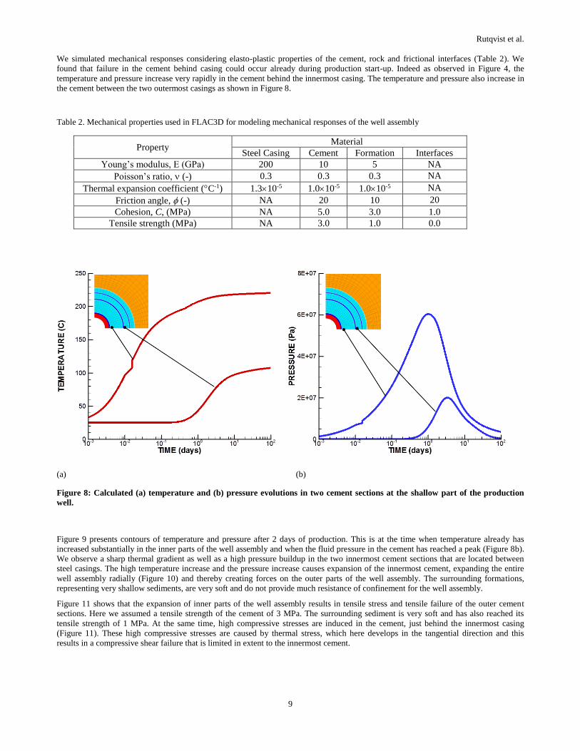
We simulated mechanical responses considering elasto-plastic properties of the cement, rock and frictional interfaces (Table 2). We

found that failure in the cement behind casing could occur already during production start-up. Indeed as observed in Figure 4, the

temperature and pressure increase very rapidly in the cement behind the innermost casing. The temperature and pressure also increase in

the cement between the two outermost casings as shown in Figure 8.

Table 2. Mechanical properties used in FLAC3D for modeling mechanical responses of the well assembly

Property Material

Steel Casing Cement Formation Interfaces

Young’s modulus, E (GPa) 200 10 5 NA

Poisson’s ratio, (-) 0.3 0.3 0.3 NA

Thermal expansion coefficient (C-1) 1.310-5 1.010-5 1.010-5 NA

Friction angle, (-) NA 20 10 20

Cohesion, C, (MPa) NA 5.0 3.0 1.0

Tensile strength (MPa) NA 3.0 1.0 0.0

(a) (b)

Figure 8: Calculated (a) temperature and (b) pressure evolutions in two cement sections at the shallow part of the production

well.

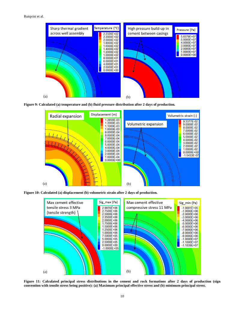
Figure 9 presents contours of temperature and pressure after 2 days of production. This is at the time when temperature already has

increased substantially in the inner parts of the well assembly and when the fluid pressure in the cement has reached a peak (Figure 8b).

We observe a sharp thermal gradient as well as a high pressure buildup in the two innermost cement sections that are located between

steel casings. The high temperature increase and the pressure increase causes expansion of the innermost cement, expanding the entire

well assembly radially (Figure 10) and thereby creating forces on the outer parts of the well assembly. The surrounding formations,

representing very shallow sediments, are very soft and do not provide much resistance of confinement for the well assembly.

Figure 11 shows that the expansion of inner parts of the well assembly results in tensile stress and tensile failure of the outer cement

sections. Here we assumed a tensile strength of the cement of 3 MPa. The surrounding sediment is very soft and has also reached its

tensile strength of 1 MPa. At the same time, high compressive stresses are induced in the cement, just behind the innermost casing

(Figure 11). These high compressive stresses are caused by thermal stress, which here develops in the tangential direction and this

results in a compressive shear failure that is limited in extent to the innermost cement.

Rutqvist et al.

10

Figure 9: Calculated (a) temperature and (b) fluid pressure distribution after 2 days of production.

Figure 10: Calculated (a) displacement (b) volumetric strain after 2 days of production.

Figure 11: Calculated principal stress distributions in the cement and rock formations after 2 days of production (sign

convention with tensile stress being positive): (a) Maximum principal effective stress and (b) minimum principal stress.

(a) (b)

(a) (b)

(a) (b)

Rutqvist et al.

11

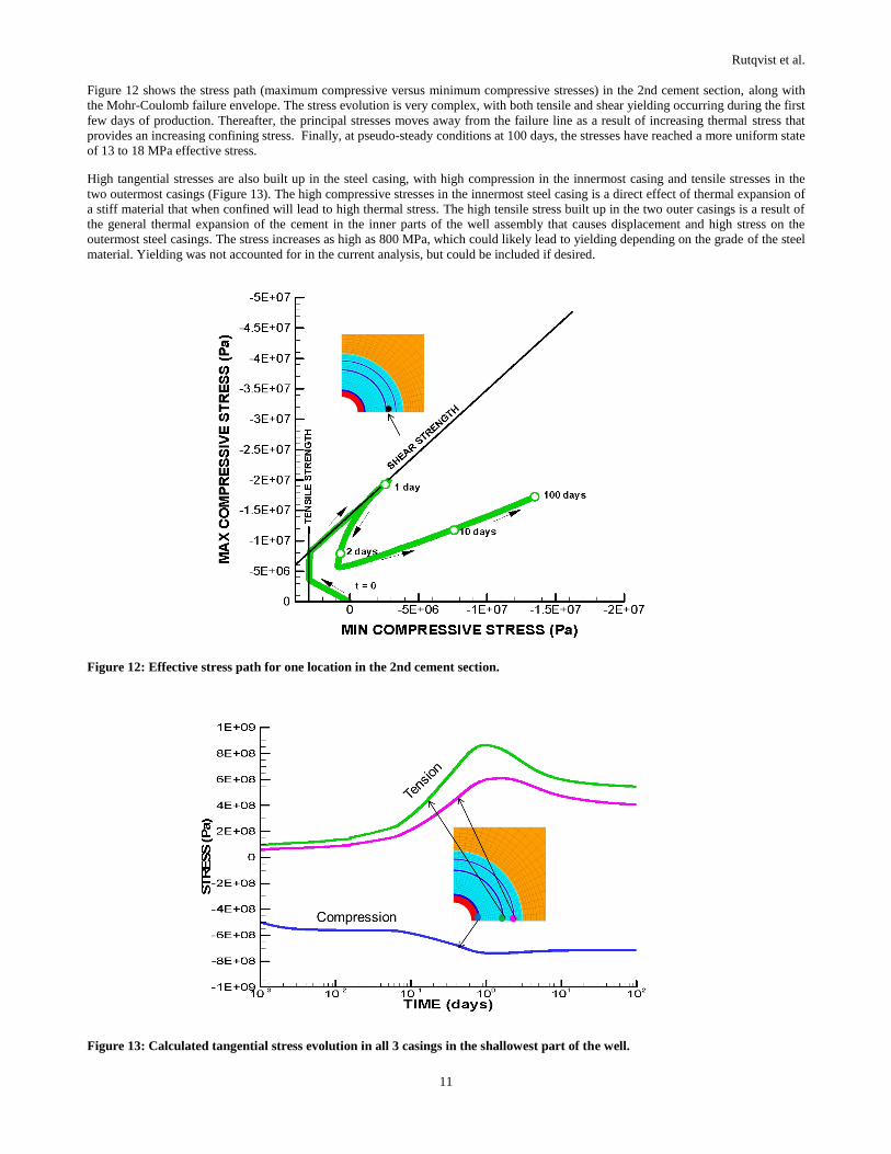
Figure 12 shows the stress path (maximum compressive versus minimum compressive stresses) in the 2nd cement section, along with

the Mohr-Coulomb failure envelope. The stress evolution is very complex, with both tensile and shear yielding occurring during the first

few days of production. Thereafter, the principal stresses moves away from the failure line as a result of increasing thermal stress that

provides an increasing confining stress. Finally, at pseudo-steady conditions at 100 days, the stresses have reached a more uniform state

of 13 to 18 MPa effective stress.

High tangential stresses are also built up in the steel casing, with high compression in the innermost casing and tensile stresses in the

two outermost casings (Figure 13). The high compressive stresses in the innermost steel casing is a direct effect of thermal expansion of

a stiff material that when confined will lead to high thermal stress. The high tensile stress built up in the two outer casings is a result of

the general thermal expansion of the cement in the inner parts of the well assembly that causes displacement and high stress on the

outermost steel casings. The stress increases as high as 800 MPa, which could likely lead to yielding depending on the grade of the steel

material. Yielding was not accounted for in the current analysis, but could be included if desired.

Figure 12: Effective stress path for one location in the 2nd cement section.

Figure 13: Calculated tangential stress evolution in all 3 casings in the shallowest part of the well.

Rutqvist et al.

12

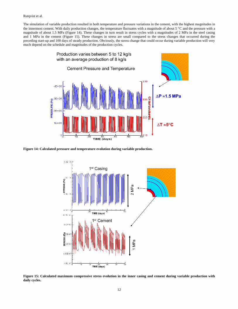
The simulation of variable production resulted in both temperature and pressure variations in the cement, with the highest magnitudes in

the innermost cement. With daily production changes, the temperature fluctuates with a magnitude of about 5 C and the pressure with a

magnitude of about 1.5 MPa (Figure 14). These changes in turn result in stress cycles with a magnitudes of 2 MPa in the steel casing

and 1 MPa in the cement (Figure 15). These changes in stress are small compared to the stress changes that occurred during the

preceding start-up and 100 days of steady production. Obviously, the stress change that could occur during variable production will very

much depend on the schedule and magnitudes of the production cycles.

Figure 14: Calculated pressure and temperature evolution during variable production.

Figure 15: Calculated maximum compressive stress evolution in the inner casing and cement during variable production with

daily cycles.

Rutqvist et al.

13

The current model simulation indicates that the cement sheath could fail already during the initial start-up of production and therefore

this would remain during the variable production. The conditions simulated in this mechanical analysis might be extreme with rapid

temperature increase and pressure buildup behind the casing. The thermal pressurization in the cement sections located between casing

might have a significant effect on well integrity. Such thermal pressurization might be avoided by increasing the production in steps so

that any pressure increase has time to bleed off. Nevertheless, even in the case of a slow increase in production flow rates, thermal

expansion of the inner parts of the well assembly will still impact the outer parts and significant loading will occur. During variable

production, the cyclic temperature and pressure changes in the cement will lead to smaller mechanical changes but could over time lead

to fatigue. These are aspects that will be analyzed with the model approach developed and demonstrated in this study.

5. CONCLUSIONS

We have investigated the effects of steady and variable geothermal production on mechanical well integrity issues using coupled

modeling of flow, heat and mechanical responses in the well assembly. The coupled modeling approach used in this analysis is based on

linking the T2Well reservoir-wellbore simulator with the FLAC3D geomechanical simulator and a detailed discretization of the well

assembly, including casing, cement, wellbore host rock, and their interfaces. We tested the applicability of this model by conducting a

series of simulations of generic steam-dominant and liquid-dominant systems of both steady and variable geothermal production. The

modeling shows that the highest thermal perturbation, ∆T, occurred in the case of a steam-dominant system in the shallow formations

beneath the ground surface near the production well. In this zone, the temperature increases quickly with production, and decays quickly

when the production rate is reduced during variable or flexible-mode operation, with the highest cyclic increase and decrease of

temperature. Moreover, temperature increases in the cement behind casing causes pressure increases due to thermal pressurization.

These temperature and pressure changes can cause non-linear mechanical responses that are dependent on the thermal expansion of the

different components of the well assembly and include effects of potential fictional sliding at interfaces and material yielding. In the

current analysis, we found that temperature changes during the initial start-up of the production could cause cement failure in the

shallowest parts of the well both in tension and compression. The coupled T2Well-FLAC3D model can be applied to better quantify

these effects for safe and sustainable production, both at base-load and flexible production modes. Future studies will involve more site-

specific data for both liquid and steam-dominant geothermal systems, including data from pilot experiments on variable production at

The Geysers geothermal field.

ACKNOWLEDGMENTS

We thank Calpine Corporation, including Julio Garcia, for generously providing well and field data for The Geysers geothermal field.

Funding for this work was provided by the California Energy Commission under the EPIC grant program (GFO-16-301) under

agreement EPC-16-022, as part of Work for Others funding from Berkeley Lab, provided by the Director, Office of Science, of the U.S.

Department of Energy under Contract No. DE-AC02-05CH11231.

REFERENCES

Garcia, J., Hartline, C., Walters, M., Wright, M., Rutqvist, J., Dobson, P.F. and Jeanne, P.: The Northwest Geysers EGS Demonstration

Project, California - Part 1: Characterization and reservoir response to injection, Geothermics, 63, (2016), 97–119.

Goyal, K.P.: Reservoir Response to Curtailment at the Geysers, Proceedings, 27th Workshop on Geothermal Reservoir Engineering,

Stanford University, Stanford, CA (2002).

Itasca Consulting Group: FLAC3D, Fast Lagrangian Analysis of Continua in 3 Dimensions, Version 5.0, Minneapolis, Minnesota,

Itasca Consulting Group (2012).

Kim, J., Tchelepi, H.A., and Juanes, R.: Stability and convergence of sequential methods for coupled flow and geomechanics: Fixed-

stress and fixed-strain splits, Comput. Methods Appl. Mech. Eng. (13-16), (2011), 1591–1606.

Pan, L., and Oldenburg, C.: T2Well—An integrated wellbore–reservoir simulator, Computers & Geosciences, 65, (2014), 46–55.

Pruess, K., Oldenburg, C., and Moridis, G.: TOUGH2 User’s Guide, Version 2.1, LBNL-43134, Lawrence Berkeley National

Laboratory, Berkeley, California (2012).

Rutqvist, J.: Status of the TOUGH-FLAC Simulator and Recent Applications Related to Coupled Fluid Flow and Crustal Deformations,

Computers & Geosciences, 37, (2011), 739–750.

Rutqvist, J. An overview of TOUGH-based geomechanics models, Computers & Geosciences, 108, (2017), 56–63.

Rutqvist, J., Jeanne, P., Dobson, P.F., Garcia, J., Hartline, C., Hutchings, L., Singh, A., Vasco, D.W., and Walters, M.: The Northwest

Geysers EGS Demonstration Project, California - Part 2: Modeling and interpretation, Geothermics, 63, (2016), 120–138.