Embed Size (px)
Citation preview
Data Frag. Model Model Summaries Stat. Model Results
Modeling of Cell Proliferation with FlowCytometry Data from CFSE-based Assays
H.T. Banks
Center for Quantitative Sciences in BiomedicineCenter for Research in Scientific Computation
Department of MathematicsNorth Carolina State University
Raleigh, NC
H.T. Banks CFSE Modeling
Data Frag. Model Model Summaries Stat. Model Results
Clay Thompson and Karyn SuttonCRSC Postdocs at NCSU
Tim SchenkelDepartment of Virology, Saarland University, Homburg, Germany
Jordi Argilaguet, Sandra Giest,Cristina Peligero, Andreas Meyerhans
ICREA Infection Biology Lab, Univ. Pompeu Fabra, Barcelona, Spain
Gennady BocharovInstitute of Numerical Mathematics, RAS, Moscow, Russia
H.T. Banks CFSE Modeling
Data Frag. Model Model Summaries Stat. Model Results
1 CFSE Data Overview
2 Initial Fragmentation Model of CFSE Data
3 Model Summaries
4 Data Statistical Model
5 Results
H.T. Banks CFSE Modeling
Data Frag. Model Model Summaries Stat. Model Results
Selected Sources and References
H.T. Banks, Frederique Charles, Marie Doumic, Karyn L. Sutton, and W. Clayton Thompson, Labelstructured cell proliferation models, Appl. Math. Letters 23 (2010), 1412–1415;doi:10.1016/j.aml.2010.07.009
H.T. Banks, Karyn L. Sutton, W. Clayton Thompson, Gennady Bocharov, Dirk Roose, Tim Schenkel, andAndreas Meyerhans, Estimation of cell proliferation dynamics using CFSE data, CRSC-TR09-17, NorthCarolina State University, August 2009; Bull. Math. Biol., 70 (2011), 116–150.
H.T. Banks, Karyn L. Sutton, W. Clayton Thompson, G. Bocharov, Marie Doumic, Tim Schenkel, JordiArgilaguet, Sandra Giest, Cristina Peligero, and Andreas Meyerhans, A new model for the estimation of cellproliferation dynamics using CFSE data, CRSC-TR11-05, North Carolina State University, Revised July2011; J. Immunological Methods, 373 (2011), 143–160; DOI:10.1016/j.jim.2011.08.014.
H.T. Banks, W. Clayton Thompson, Jordi Argilaguet, Cristina Peligero, and Andreas Meyerhans, Adivision-dependent compartmental model for computing cell numbers in CFSE-based lymphocyteproliferation assays, CRSC-TR12-03, N. C. State University, Raleigh, NC, January, 2012; Math. Biosci.Engr., to appear.
H.T. Banks and W. Clayton Thompson, Mathematical models of dividing cell populations: Application toCFSE data, CRSC-TR12-10, N. C. State University, Raleigh, NC, April, 2012; Journal on MathematicalModelling of Natural Phenomena, to appear.
H.T. Banks and W. Clayton Thompson, A division-dependent compartmental model with cyton andintracellular label dynamics, CRSC-TR12-12, N. C. State University, Raleigh, NC, May, 2012; Intl. J. of Pureand Applied Math., 77 (2012), 119–147.
H.T. Banks CFSE Modeling
Data Frag. Model Model Summaries Stat. Model Results
Selected Sources and References
H.T. Banks, Amanda Choi, Tori Huffman, John Nardini, Laura Poag and W. Clayton Thompson, ModelingCFSE label decay in flow cytometry data, CRSC-TR12-20, N. C. State University, Raleigh, NC, November,2012; Applied Mathematical Letters, (2103), doi:10.1016/j.aml.2012.12.010.
H.T. Banks, D. F. Kapraun, W. Clayton Thompson, Cristina Peligero, Jordi Argilaguet and AndreasMeyerhans, A novel statistical analysis and interpretation of flow cytometry data, CRSC-TR12-23, N. C.State University, Raleigh, NC, December, 2012; J. Biological Dynamics, submitted.
A.V. Gett and P.D. Hodgkin, A cellular calculus for signal integration by T cells, Nature Immunology 1 (2000),239–244.
E.D. Hawkins, Mirja Hommel, M.L Turner, Francis Battye, J Markham and P.D Hodgkin, Measuringlymphocyte proliferation, survival and differentiation using CFSE time-series data, Nature Protocols, 2(2007), 2057–2067.
E.D. Hawkins, M.L. Turner, M.R. Dowling, C. van Gend, and P.D. Hodgkin, A model of immune regulation asa consequence of randomized lymphocyte division and death times, Proc. Natl. Acad. Sci., 104 (2007),5032–5037.
T. Luzyanina, D. Roose, T. Schenkel, M. Sester, S. Ehl, A. Meyerhans, and G. Bocharov, Numericalmodelling of label-structured cell population growth using CFSE distribution data, Theoretical Biology andMedical Modelling 4 (2007), Published Online.
C. Parish, Fluorescent dyes for lymphocyte migration and proliferation studies, Immunology and Cell Biol.77 (1999), 499–508.
H.T. Banks CFSE Modeling
Data Frag. Model Model Summaries Stat. Model Results
Selected Sources and References
B. Quah, H. Warren and C. Parish, Monitoring lymphocyte proliferation in vitro and in vivo with theintracellular fluorescent dye carboxyfluorescein diacetate succinimidyl ester, Nature Protocols 2:9 (2007),2049–2056.
D. Schittler, J. Hasenauer, and F. Allgower, A generalized model for cell proliferation: Integrating divisionnumbers and label dynamics, Proc. Eighth International Workshop on Computational Systems Biology(WCSB 2011), June 2001, Zurich, Switzerland, p. 165–168.
J. Hasenauer, D. Schittler and F. Allgower, Analysis and simulation of division- and label-structuredpopulation models: A new tool to analyze proliferation assays, Bull. Math. Biol., 74 (2012), 2692–2732.
H.T. Banks CFSE Modeling
Data Frag. Model Model Summaries Stat. Model Results
Scientific Goals
Long-term collaboration between NCSU and UPFMonitor cell division and differentiation
Assess polyfunctionalityInvestigate immunospecific extracellular signaling pathwaysIdentify correlated and (ideally) causal relationshipsbetween immune mechanisms
Quantitative measure of ‘dynamic responsiveness’
Link observed (cellular) behaviors to clinical outcomes;improve clinical outcomes
The ‘central problem in immunology’ (according to G.Bocharov): to understand the ‘cellular and molecularmechanisms that control the ability of the immune systemto mount a protective response against pathogen-derivedforeign antigens, but avoid a pathological response toself-antigens’
H.T. Banks CFSE Modeling
Data Frag. Model Model Summaries Stat. Model Results
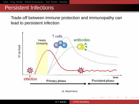
Persistent Infections
Trade-off between immune protection and immunopathy canlead to persistent infection
(A. Meyerhans)
H.T. Banks CFSE Modeling
Data Frag. Model Model Summaries Stat. Model Results
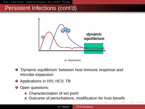
Persistent Infections (cont’d)
(A. Meyerhans)
‘Dynamic equilibrium’ between host immune response andmicrobe expansion
Applications in HIV, HCV, TB
Open questions:Characterization of set pointOutcome of perturbations, modification for host benefit
H.T. Banks CFSE Modeling
Data Frag. Model Model Summaries Stat. Model Results
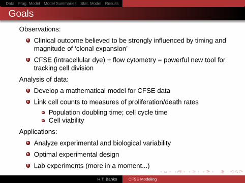
Goals
Observations:
Clinical outcome believed to be strongly influenced by timing andmagnitude of ‘clonal expansion’
CFSE (intracellular dye) + flow cytometry = powerful new tool fortracking cell division
Analysis of data:
Develop a mathematical model for CFSE data
Link cell counts to measures of proliferation/death rates
Population doubling time; cell cycle timeCell viability
Applications:
Analyze experimental and biological variability
Optimal experimental design
Lab experiments (more in a moment...)
H.T. Banks CFSE Modeling

Data Frag. Model Model Summaries Stat. Model Results
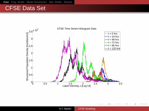
CFSE Data Set
0 0.5 1 1.5 2 2.5 3 3.50
0.5
1
1.5
2
2.5
3
3.5x 10⁵ CFSE Time Series Histogram Data
Label Intensity z [Log UI]
Str
uctu
red
Pop
ulat
ion
Den
sity
[num
bers
/UI]
t = 0 hrst = 24 hrst = 48 hrst = 72 hrst = 96 hrst = 120 hrs
H.T. Banks CFSE Modeling
Data Frag. Model Model Summaries Stat. Model Results
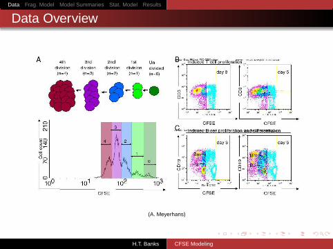
Data Overview
(A. Meyerhans)
H.T. Banks CFSE Modeling
Data Frag. Model Model Summaries Stat. Model Results
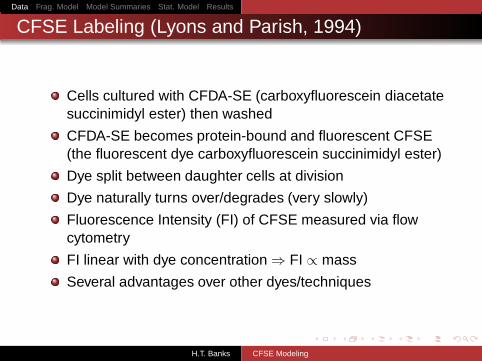
CFSE Labeling (Lyons and Parish, 1994)
Cells cultured with CFDA-SE (carboxyfluorescein diacetatesuccinimidyl ester) then washed
CFDA-SE becomes protein-bound and fluorescent CFSE(the fluorescent dye carboxyfluorescein succinimidyl ester)
Dye split between daughter cells at division
Dye naturally turns over/degrades (very slowly)
Fluorescence Intensity (FI) of CFSE measured via flowcytometry
FI linear with dye concentration ⇒ FI ∝ mass
Several advantages over other dyes/techniques
H.T. Banks CFSE Modeling
Data Frag. Model Model Summaries Stat. Model Results
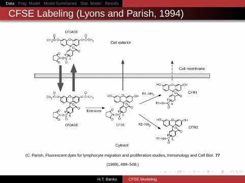
CFSE Labeling (Lyons and Parish, 1994)
(C. Parish, Fluorescent dyes for lymphocyte migration and proliferation studies, Immunology and Cell Biol. 77
(1999), 499–508.)
H.T. Banks CFSE Modeling
Data Frag. Model Model Summaries Stat. Model Results
CFSE Data Set
0 0.5 1 1.5 2 2.5 3 3.50
0.5
1
1.5
2
2.5
3
3.5x 10⁵ CFSE Time Series Histogram Data
Label Intensity z [Log UI]
Str
uctu
red
Pop
ulat
ion
Den
sity
[num
bers
/UI]
t = 0 hrst = 24 hrst = 48 hrst = 72 hrst = 96 hrst = 120 hrs
H.T. Banks CFSE Modeling
Data Frag. Model Model Summaries Stat. Model Results
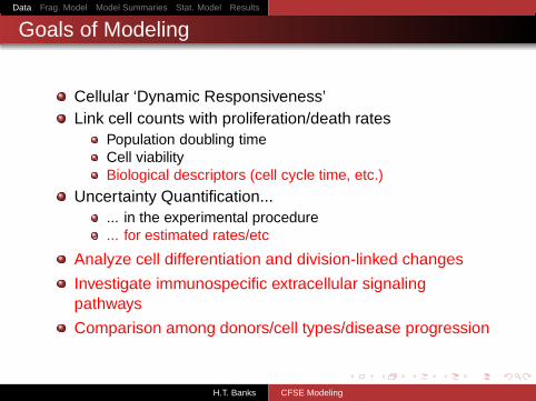
Goals of Modeling
Cellular ‘Dynamic Responsiveness’Link cell counts with proliferation/death rates
Population doubling timeCell viabilityBiological descriptors (cell cycle time, etc.)
Uncertainty Quantification...... in the experimental procedure... for estimated rates/etc
Analyze cell differentiation and division-linked changes
Investigate immunospecific extracellular signalingpathways
Comparison among donors/cell types/disease progression
H.T. Banks CFSE Modeling
Data Frag. Model Model Summaries Stat. Model Results
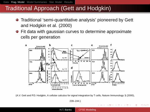
Traditional Approach (Gett and Hodgkin)
Traditional ‘semi-quantitative analysis’ pioneered by Gettand Hodgkin et al. (2000)Fit data with gaussian curves to determine approximatecells per generation
(A.V. Gett and P.D. Hodgkin, A cellular calculus for signal integration by T cells, Nature Immunology 1 (2000),
239–244.)
H.T. Banks CFSE Modeling
Data Frag. Model Model Summaries Stat. Model Results
Traditional Approach (cont’d)
Gett-Hodgkin method quick, easy to implement, usefulcomparisons between data sets (e.g. stimulationconditions)
Compatible with ODE, DDE models; ‘indirect fitting’ forparameter estimationGeneralizations, extensions, and various other modelingefforts
Smith-Martin model (with generalizations)Cyton modelBranching process models
H.T. Banks CFSE Modeling
Data Frag. Model Model Summaries Stat. Model Results
Label-Structured Model
All previous work with cell numbers determined bydeconvolutionAlternatively, we propose to fit the CFSE histogram datadirectly
Capture full behavior of the population densityNo assumption on the shape of CFSE uptake/distribution
Histogram presentation of cytometry data makesstructured population models a natural choice (as in age,size, etc) except here structure label is “CFSE content orintensity”
Key ideas first formulated by Luzyanina, Bocharov, et al.,2007FI (or log FI) ⇔ Division Number
H.T. Banks CFSE Modeling
Data Frag. Model Model Summaries Stat. Model Results
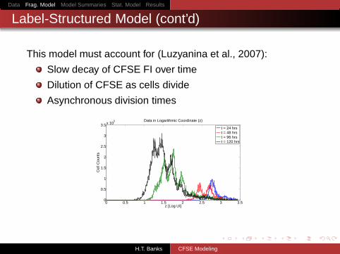
Label-Structured Model (cont’d)
This model must account for (Luzyanina et al., 2007):
Slow decay of CFSE FI over time
Dilution of CFSE as cells divide
Asynchronous division times
0 0.5 1 1.5 2 2.5 3 3.50
0.5
1
1.5
2
2.5
3
3.5x 10⁵ Data in Logarithmic Coordinate (z)
z [Log UI]
Cel
l Cou
nts
t = 24 hrst = 48 hrst = 96 hrst = 120 hrs
H.T. Banks CFSE Modeling
Data Frag. Model Model Summaries Stat. Model Results
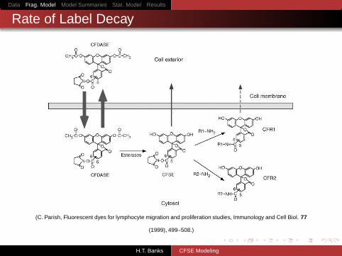
Rate of Label Decay
(C. Parish, Fluorescent dyes for lymphocyte migration and proliferation studies, Immunology and Cell Biol. 77
(1999), 499–508.)
H.T. Banks CFSE Modeling
Data Frag. Model Model Summaries Stat. Model Results
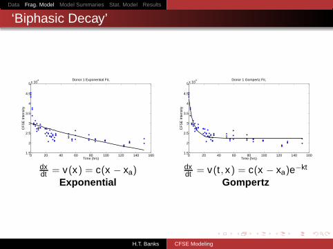
‘Biphasic Decay’
0 20 40 60 80 100 120 140 1601.5
2
2.5
3
3.5
4
4.5
5x 10⁴ Donor 1 Exponential Fit,
Time (hrs)
CF
SE
Inte
nsity
dxdt = v(x) = c(x − xa)
Exponential
0 20 40 60 80 100 120 140 1601.5
2
2.5
3
3.5
4
4.5
5x 10⁴ Donor 1 Gompertz Fit,
Time (hrs)
CF
SE
Inte
nsity
dxdt = v(t , x) = c(x − xa)e−kt
Gompertz
H.T. Banks CFSE Modeling
Data Frag. Model Model Summaries Stat. Model Results
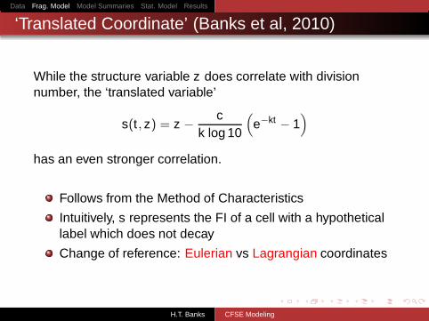
‘Translated Coordinate’ (Banks et al, 2010)
While the structure variable z does correlate with divisionnumber, the ‘translated variable’
s(t , z) = z − ck log 10
(
e−kt − 1)
has an even stronger correlation.
Follows from the Method of Characteristics
Intuitively, s represents the FI of a cell with a hypotheticallabel which does not decay
Change of reference: Eulerian vs Lagrangian coordinates
H.T. Banks CFSE Modeling
Data Frag. Model Model Summaries Stat. Model Results
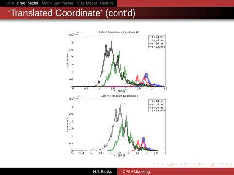
‘Translated Coordinate’ (cont’d)
0 0.5 1 1.5 2 2.5 3 3.50
0.5
1
1.5
2
2.5
3
3.5x 10⁵ Data in Logarithmic Coordinate (z)
z [Log UI]
Cel
l Cou
nts
t = 24 hrst = 48 hrst = 96 hrst = 120 hrs
−1 −0.5 0 0.5 1 1.5 2 2.5 3 3.5 40
0.5
1
1.5
2
2.5
3
3.5x 10⁵
X: 1.592Y: 3.109e+05
Data in Translated Coordinate s
s [Log UI]
Cel
l Cou
nts
t = 24 hrst = 48 hrst = 96 hrst = 120 hrs
H.T. Banks CFSE Modeling
Data Frag. Model Model Summaries Stat. Model Results
Fragmentation Model Summary
Model is capable of precisely fitting the observed data
c, k , xa estimated consistently (as α and β nodes change),though subject to high experimental variability
‘Translated coordinate’ very strongly correlated withdivision number
Time-dependence of the proliferation rate is an essentialfeature of the model
Biologically relevant average values of proliferation anddeath (in terms of number of divisions undergone) areeasily computable.But...(Aggregate Data/Aggregate Dynamics)
Still cannot compute cell numbers and cohort rateparametersData overlap affecting estimated rates (?)Large number of parameters necessary
H.T. Banks CFSE Modeling
Data Frag. Model Model Summaries Stat. Model Results
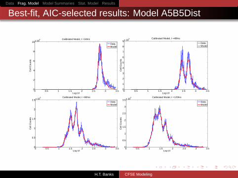
Best-fit, AIC-selected results: Model A5B5Dist
0 0.5 1 1.5 2 2.5 3 3.50
2
4
6
8
10x 104 Calibrated Model, t =24hrs
Log UI
Cel
l Cou
nts
DataModel
0 0.5 1 1.5 2 2.5 3 3.50
1
2
3
4
5
6
7
8
9x 10⁴ Calibrated Model, t =48hrs
Log UI
Cel
l Cou
nts
DataModel
0 0.5 1 1.5 2 2.5 3 3.50
0.5
1
1.5
2
2.5x 10⁵ Calibrated Model, t =96hrs
Log UI
Cel
l Cou
nts
DataModel
0 0.5 1 1.5 2 2.5 3 3.50
0.5
1
1.5
2
2.5
3
3.5x 10⁵ Calibrated Model, t =120hrs
Log UI
Cel
l Cou
nts
DataModel
H.T. Banks CFSE Modeling
Data Frag. Model Model Summaries Stat. Model Results
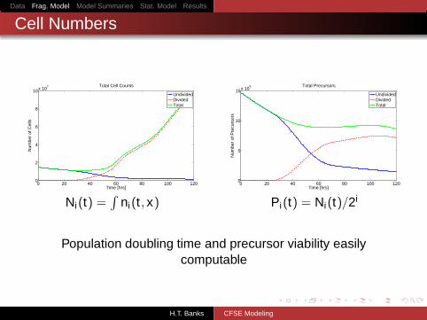
Cell Numbers
0 20 40 60 80 100 1200
2
4
6
8
10x 107 Total Cell Counts
Time [hrs]
Num
ber
of C
ells
UndividedDividedTotal
Ni(t) =∫
ni(t , x)
0 20 40 60 80 100 1200
5
10
15x 106 Total Precursors
Time [hrs]
Num
ber
of P
recu
rsor
s
UndividedDividedTotal
Pi(t) = Ni(t)/2i
Population doubling time and precursor viability easilycomputable
H.T. Banks CFSE Modeling
Data Frag. Model Model Summaries Stat. Model Results
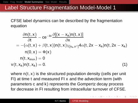
Label Structure Fragmentation Model-Model 1
CFSE label dynamics can be described by the fragmentationequation
∂n(t , x)∂t
− ce−kt ∂[(x − xa)n(t , x)]∂x
= −(α(t , x) + β(t , x))n(t , x)χ[xa ,x∗]4α(t ,2x − xa)n(t ,2x − xa)
n(0, x) = Φ(x)
n(t , xmax) = 0
v(t , xa)n(t , xa) = 0. (1)
where n(t , x) is the structured population density (cells per unitFI) at time t and measured FI x and the advection term (withparameters c and k) represents the Gompertz decay processfor decrease in FI resulting from intracellular turnover of CFSE.
H.T. Banks CFSE Modeling
Data Frag. Model Model Summaries Stat. Model Results
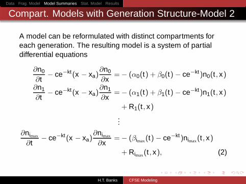
Compart. Models with Generation Structure-Model 2
A model can be reformulated with distinct compartments foreach generation. The resulting model is a system of partialdifferential equations
∂n0
∂t− ce−kt(x − xa)
∂n0
∂x=− (α0(t) + β0(t) − ce−kt)n0(t , x)
∂n1
∂t− ce−kt(x − xa)
∂n1
∂x=− (α1(t) + β1(t) − ce−kt)n1(t , x)
+ R1(t , x)...
∂nimax
∂t− ce−kt(x − xa)
∂nimax
∂x=− (βimax
(t) − ce−kt)nimax(t , x)
+ Rimax(t , x), (2)
H.T. Banks CFSE Modeling
Data Frag. Model Model Summaries Stat. Model Results
Compartmental Models-Model 2
Here ni(t , x) is structured population density for cells havingundergone i divisions. The recruitment terms describe thesymmetric division of CFSE upon mitosis. Given byRi(t , x) = 4αi−1(t)ni−1(t ,2x − xa). Boundary and initialconditions same as in (1).
Observe that, because the number of divisions undergone hasnow been explicitly identified by the subscripted generationnumber, no longer necessary for division and death rates todepend upon measured fluorescence intensity.
H.T. Banks CFSE Modeling
Data Frag. Model Model Summaries Stat. Model Results
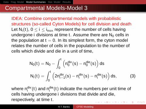
Compartmental Models-Model 3
IDEA: Combine compartmental models with probabilisticstructures (so-called Cyton Models) for cell division and deathLet Ni(t), 0 ≤ i ≤ imax represent the number of cells havingundergone i divisions at time t . Assume there are N0 cells inthe population at t = 0. In its simplest form, the cyton modelrelates the number of cells in the population to the number ofcells which divide and die in a unit of time,
N0(t) = N0 −∫ t
0
(
ndiv0 (s)− ndie
0 (s))
ds
Ni(t) =∫ t
0
(
2ndivi−1(s)− ndiv
i (s)− ndiei (s)
)
ds, (3)
where ndivi (t) and ndie
i (t) indicate the numbers per unit time ofcells having undergone i divisions that divide and die,respectively, at time t .
H.T. Banks CFSE Modeling
Data Frag. Model Model Summaries Stat. Model Results
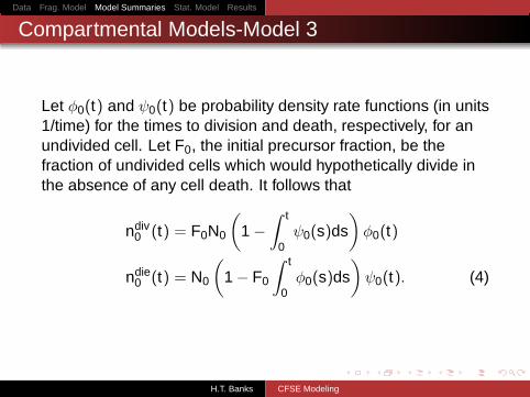
Compartmental Models-Model 3
Let φ0(t) and ψ0(t) be probability density rate functions (in units1/time) for the times to division and death, respectively, for anundivided cell. Let F0, the initial precursor fraction, be thefraction of undivided cells which would hypothetically divide inthe absence of any cell death. It follows that
ndiv0 (t) = F0N0
(
1 −∫ t
0ψ0(s)ds
)
φ0(t)
ndie0 (t) = N0
(
1 − F0
∫ t
0φ0(s)ds
)
ψ0(t). (4)
H.T. Banks CFSE Modeling
Data Frag. Model Model Summaries Stat. Model Results
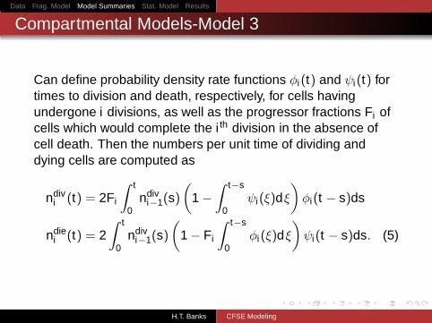
Compartmental Models-Model 3
Can define probability density rate functions φi(t) and ψi(t) fortimes to division and death, respectively, for cells havingundergone i divisions, as well as the progressor fractions Fi ofcells which would complete the i th division in the absence ofcell death. Then the numbers per unit time of dividing anddying cells are computed as
ndivi (t) = 2Fi
∫ t
0ndiv
i−1(s)(
1 −∫ t−s
0ψi(ξ)dξ
)
φi(t − s)ds
ndiei (t) = 2
∫ t
0ndiv
i−1(s)(
1 − Fi
∫ t−s
0φi(ξ)dξ
)
ψi(t − s)ds. (5)
H.T. Banks CFSE Modeling
Data Frag. Model Model Summaries Stat. Model Results
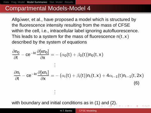
Compartmental Models-Model 4
Allgower, et al., have proposed a model which is structured bythe fluorescence intensity resulting from the mass of CFSEwithin the cell, i.e., intracellular label ignoring autofluorescence.This leads to a system for the mass of fluorescence n(t , x)described by the system of equations
∂n0
∂t− ce−kt ∂[xn0]
∂x=− (α0(t) + β0(t))n0(t , x)
...
∂ni
∂t− ce−kt ∂[xni ]
∂x=− (αi(t) + βi(t))ni (t , x) + 4αi−1(t)ni−1(t ,2x)
(6)...
with boundary and initial conditions as in (1) and (2).
H.T. Banks CFSE Modeling
Data Frag. Model Model Summaries Stat. Model Results
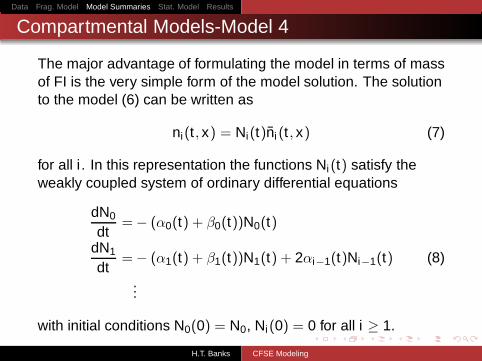
Compartmental Models-Model 4
The major advantage of formulating the model in terms of massof FI is the very simple form of the model solution. The solutionto the model (6) can be written as
ni(t , x) = Ni(t)ni (t , x) (7)
for all i . In this representation the functions Ni(t) satisfy theweakly coupled system of ordinary differential equations
dN0
dt=− (α0(t) + β0(t))N0(t)
dN1
dt=− (α1(t) + β1(t))N1(t) + 2αi−1(t)Ni−1(t) (8)
...
with initial conditions N0(0) = N0, Ni(0) = 0 for all i ≥ 1.
H.T. Banks CFSE Modeling
Data Frag. Model Model Summaries Stat. Model Results
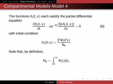
Compartmental Models-Model 4
The functions ni(t , x) each satisfy the partial differentialequation
∂ni(t , x)∂t
− ce−kt ∂[xni(t , x)]∂x
= 0 (9)
with initial condition
ni(0, x) =2iΦ(2ix)
N0.
Note that, by definition,
N0 =
∫
∞
0Φ(ξ)dξ.
H.T. Banks CFSE Modeling
Data Frag. Model Model Summaries Stat. Model Results
Compartmental Models-Model 4
Let ni(t , x) be the structured density relative to the measuredfluorescence (x is related to x by the addition of cellularautofluorescence). To account for autofluorescence andbecause autofluorescence may vary from cell to cell in thepopulation, this is most accurately treated by computing theconvolution integral
n(t , x) =∫
∞
0n(t , x)p(t , x − x)dx , (10)
where p(t , x) is (for each fixed time t) a probability densityfunction describing the distribution of autofluorescence in thepopulation.
H.T. Banks CFSE Modeling
Data Frag. Model Model Summaries Stat. Model Results
Compartmental Models-Model 4
So finally we consider the system of equations
∂n0
∂t− ce−kt ∂[xn0]
∂x=(
ndiv0 (t)− ndie
0 (t))
n0(t , x)
∂n1
∂t− ce−kt ∂[xn1]
∂x=(
2ndiv0 (t) − ndiv
1 (t) − ndie1 (t)
)
n1(t , x)
(11)...
where the definitions of ndiv0 (t), ndie
0 (t), ndivi (t) and ndie
i (t) aregiven in Equations (4) - (5).
H.T. Banks CFSE Modeling

Data Frag. Model Model Summaries Stat. Model Results
Compartmental Models-Model 4
This model, which is based on simple mass balance, can besolved by factorization (7) as before; the label densities n(t , x)are readily computed according to Equation (9), and the cellnumbers are now provided by the cyton model as discussedabove. Thus the new model (11) is capable of accuratelydescribing the evolving generation structure of a population ofcells while also accounting for the manner in which the CFSEprofile of the population changes in time. The model is easilyrelatable to biologically meaningful parameters (times todivision and death) and can be solved efficiently so that it iseminently suitable for use in an inverse problem.
H.T. Banks CFSE Modeling
Data Frag. Model Model Summaries Stat. Model Results
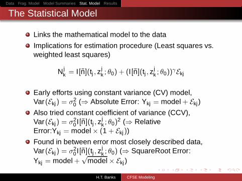
The Statistical Model
Links the mathematical model to the data
Implications for estimation procedure (Least squares vs.weighted least squares)
N jk = I[n](tj , z
jk ; θ0) + (I[n](tj , z
jk ; θ0))
γEkj
Early efforts using constant variance (CV) model,Var(Ekj) = σ2
0 (⇒ Absolute Error: Ykj = model + Ekj )
Also tried constant coefficient of variance (CCV),Var(Ekj) = σ2
0I[n](tj , zjk ; θ0)
2 (⇒ RelativeError:Ykj = model × (1 + Ekj))
Found in between error most closely described data,Var(Ekj) = σ2
0I[n](tj , zjk ; θ0) (⇒ SquareRoot Error:
Ykj = model +√
model × Ekj )
H.T. Banks CFSE Modeling
Data Frag. Model Model Summaries Stat. Model Results
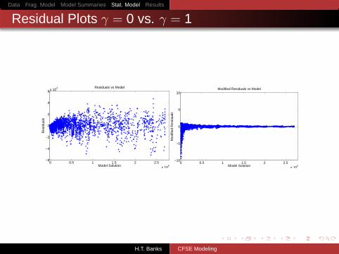
Residual Plots γ = 0 vs. γ = 1
0 0.5 1 1.5 2 2.5x 10
5
−6
−4
−2
0
2
4
6x 10⁴ Residuals vs Model
Model Solution
Res
idua
ls
0 0.5 1 1.5 2 2.5x 10
5
−10
−5
0
5
10Modified Residuals vs Model
Model Solution
Mod
ified
Res
idua
ls
H.T. Banks CFSE Modeling
Data Frag. Model Model Summaries Stat. Model Results
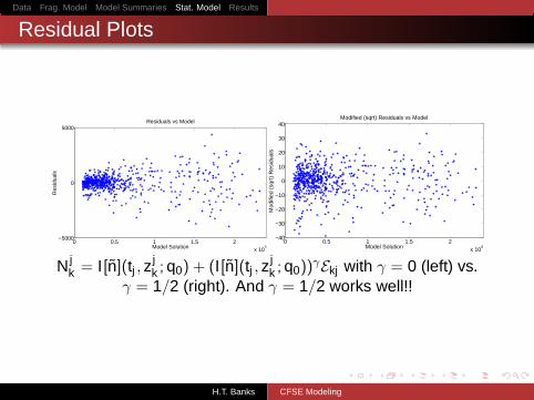
Residual Plots
0 0.5 1 1.5 2x 10
4
−5000
0
5000Residuals vs Model
Model Solution
Res
idua
ls
0 0.5 1 1.5 2x 10
4
−40
−30
−20
−10
0
10
20
30
40Modified (sqrt) Residuals vs Model
Model Solution
Mod
ified
(sq
rt)
Res
idua
lsN j
k = I[n](tj , zjk ;q0) + (I[n](tj , z
jk ;q0))
γEkj with γ = 0 (left) vs.γ = 1/2 (right). And γ = 1/2 works well!!
H.T. Banks CFSE Modeling
Data Frag. Model Model Summaries Stat. Model Results
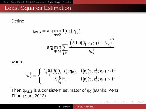
Least Squares Estimation
Define
qWLS = arg minq∈Q
J(q; {λj})
= arg minq∈Q
∑
j ,k
(
λj I[n](tj , zk ;q)− N jk
)2
w jk
where
w jk =
λjBbj
I[n](tj , zjk ;q0), I[n](tj , z
jk ;q0) > I∗
λjBbj
I∗, I[n](tj , zjk ;q0) ≤ I∗
.
Then qWLS is a consistent estimator of q0 (Banks, Kenz,Thompson, 2012)
H.T. Banks CFSE Modeling
Data Frag. Model Model Summaries Stat. Model Results
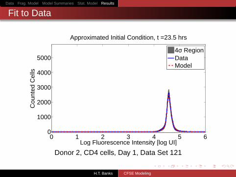
Fit to Data
0 1 2 3 4 5 60
1000
2000
3000
4000
5000
Approximated Initial Condition, t =23.5 hrs
Log Fluorescence Intensity [log UI]
Cou
nted
Cel
ls
4σ RegionDataModel
Donor 2, CD4 cells, Day 1, Data Set 121
H.T. Banks CFSE Modeling
Data Frag. Model Model Summaries Stat. Model Results
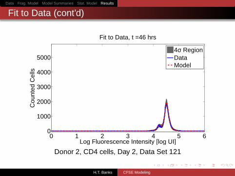
Fit to Data (cont’d)
0 1 2 3 4 5 60
1000
2000
3000
4000
5000
Fit to Data, t =46 hrs
Log Fluorescence Intensity [log UI]
Cou
nted
Cel
ls
4σ RegionDataModel
Donor 2, CD4 cells, Day 2, Data Set 121
H.T. Banks CFSE Modeling
Data Frag. Model Model Summaries Stat. Model Results
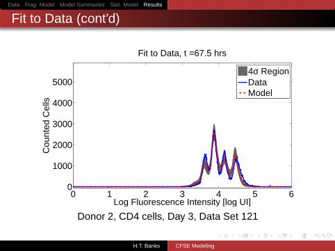
Fit to Data (cont’d)
0 1 2 3 4 5 60
1000
2000
3000
4000
5000
Fit to Data, t =67.5 hrs
Log Fluorescence Intensity [log UI]
Cou
nted
Cel
ls
4σ RegionDataModel
Donor 2, CD4 cells, Day 3, Data Set 121
H.T. Banks CFSE Modeling
Data Frag. Model Model Summaries Stat. Model Results
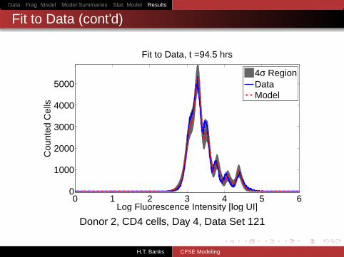
Fit to Data (cont’d)
0 1 2 3 4 5 60
1000
2000
3000
4000
5000
Fit to Data, t =94.5 hrs
Log Fluorescence Intensity [log UI]
Cou
nted
Cel
ls
4σ RegionDataModel
Donor 2, CD4 cells, Day 4, Data Set 121
H.T. Banks CFSE Modeling
Data Frag. Model Model Summaries Stat. Model Results
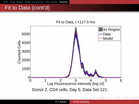
Fit to Data (cont’d)
0 1 2 3 4 5 60
1000
2000
3000
4000
5000
Fit to Data, t =117.5 hrs
Log Fluorescence Intensity [log UI]
Cou
nted
Cel
ls
4σ RegionDataModel
Donor 2, CD4 cells, Day 5, Data Set 121
H.T. Banks CFSE Modeling
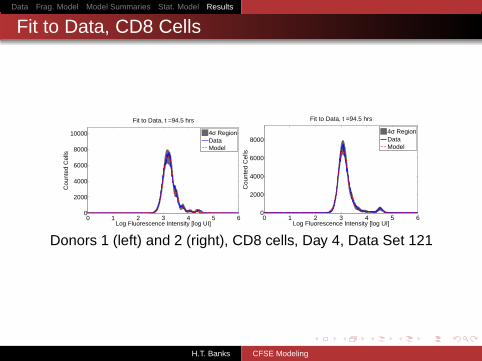
Data Frag. Model Model Summaries Stat. Model Results
Fit to Data, CD8 Cells
0 1 2 3 4 5 60
2000
4000
6000
8000
10000
Fit to Data, t =94.5 hrs
Log Fluorescence Intensity [log UI]
Cou
nted
Cel
ls
4σ RegionDataModel
0 1 2 3 4 5 60
2000
4000
6000
8000
Fit to Data, t =94.5 hrs
Log Fluorescence Intensity [log UI]
Cou
nted
Cel
ls
4σ RegionDataModel
Donors 1 (left) and 2 (right), CD8 cells, Day 4, Data Set 121
H.T. Banks CFSE Modeling
Data Frag. Model Model Summaries Stat. Model Results
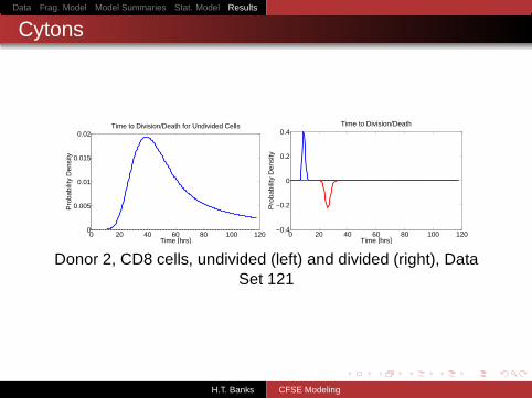
Cytons
0 20 40 60 80 100 1200
0.005
0.01
0.015
0.02Time to Division/Death for Undivided Cells
Time [hrs]
Pro
babi
lity
Den
sity
0 20 40 60 80 100 120−0.4
−0.2
0
0.2
0.4Time to Division/Death
Time [hrs]
Pro
babi
lity
Den
sity
Donor 2, CD8 cells, undivided (left) and divided (right), DataSet 121
H.T. Banks CFSE Modeling
Data Frag. Model Model Summaries Stat. Model Results
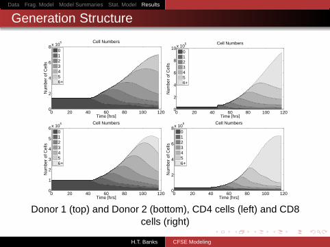
Generation Structure
0 20 40 60 80 100 1200
2
4
6
8x 10⁵
Time [hrs]
Num
ber
of C
ells
Cell Numbers
0123456+
0 20 40 60 80 100 1200
2
4
6
8
10x 105
Time [hrs]
Num
ber
of C
ells
Cell Numbers
0123456+
0 20 40 60 80 100 1200
1
2
3
4
5
6x 10⁵
Time [hrs]
Num
ber
of C
ells
Cell Numbers
0123456+
0 20 40 60 80 100 1200
2
4
6
8x 10⁵
Time [hrs]
Num
ber
of C
ells
Cell Numbers
0123456+
Donor 1 (top) and Donor 2 (bottom), CD4 cells (left) and CD8cells (right)
H.T. Banks CFSE Modeling
Data Frag. Model Model Summaries Stat. Model Results
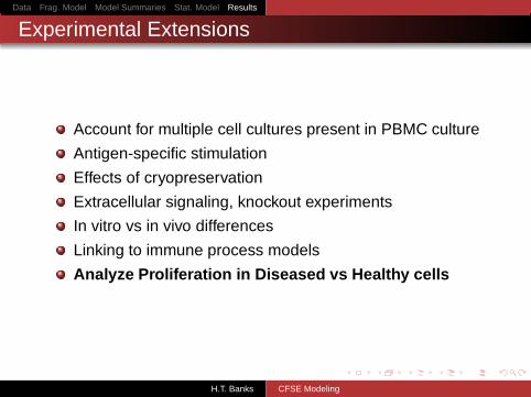
Experimental Extensions
Account for multiple cell cultures present in PBMC culture
Antigen-specific stimulation
Effects of cryopreservation
Extracellular signaling, knockout experiments
In vitro vs in vivo differences
Linking to immune process models
Analyze Proliferation in Diseased vs Healthy cells
H.T. Banks CFSE Modeling
Data Frag. Model Model Summaries Stat. Model Results
Acknowledgements
National Institute of Allergy and Infectious Disease grant NIAID9R01AI071915
U.S. Air Force Office of Scientific Research under grantAFOSR-FA9550-09-1-0226
H.T. Banks CFSE Modeling