Modeling Multiallelic Selection Using a ... - Wakeley Lab

Copyright � 2009 by the Genetics Society of AmericaDOI: 10.1534/genetics.108.089474

Modeling Multiallelic Selection Using a Moran Model

Christina A. Muirhead1 and John Wakeley

Department of Organismic and Evolutionary Biology, Harvard University, Cambridge, Massachusetts 02138

Manuscript received March 21, 2008Accepted for publication May 18, 2009

ABSTRACT

We present a Moran-model approach to modeling general multiallelic selection in a finite populationand show how it may be used to develop theoretical models of biological systems of balancing selectionsuch as plant gametophytic self-incompatibility loci. We propose new expressions for the stationarydistribution of allele frequencies under selection and use them to show that the continuous-time Markovchain describing allele frequency change with exchangeable selection and Moran-model reproduction isreversible. We then use the reversibility property to derive the expected allele frequency spectrum in afinite population for several general models of multiallelic selection. Using simulations, we show that ourapproach is valid over a broader range of parameters than previous analyses of balancing selection basedon diffusion approximations to the Wright–Fisher model of reproduction. Our results can be applied toany model of multiallelic selection in which fitness is solely a function of allele frequency.

NATURAL selection has long been a topic of interestin population genetics, yet the stochastic theory of

genes under selection remains underdeveloped com-pared to the theory of neutral genes. Due to theinterplay of stochastic and deterministic forces, modelsof selection present analytical challenges beyond thoseof neutral models, although a great deal of progress hasbeen made with models that use diffusion approxima-tions to a Wright–Fisher model of reproduction.Diffusion approximations with selection are, however,sometimes difficult to employ and always requireassumptions about population parameters for tractabil-ity. These limitations suggest that there may be value indeveloping new methods of solving the problem ofselection in a finite population, and here we do so usinga Moran model of reproduction in place of the familiarWright–Fisher model. Our approach has two majoradvantages over previous models: general applicabilityto a wide variety of selection models and accuracy overa broad range of parameter values. In this work, wepropose new expressions for the full stationary distri-butions of allele frequencies under multiallelic selec-tion, as well as expressions for average allele frequencydistributions.

We restrict our attention to exchangeable models ofselection, meaning that relabeling the alleles will notchange selective outcomes and thus that selection willbe a function of allele frequency rather than alleleidentity. Many models of selection can be transformedinto frequency-dependent forms (Denniston and

Crow 1990), and some common models of selectionhave the desired property of exchangeability. Forexample, symmetric overdominant selection, in whichheterozygotes have a selective advantage over homozy-gotes but the specific genotype of homozygote orheterozygote has no further selective effect, can beexpressed as frequency-dependent selection on individ-ual (exchangeable) alleles, although the direct selec-tion is actually on diploid genotypes. Many otherproposed models of multiallelic balancing selection,in which substantial variation is maintained by selec-tion, can be viewed in this way. Such models have beenof particular interest because of the potential applica-tion to highly multiallelic systems found in nature, suchas self-incompatibility (SI) loci in plants and the majorhistocompatibility complex (MHC) loci in vertebrates,and the desire to analyze these systems is a motivationfor the present work. We now review some of thepopulation genetic theory related to these systems.

Early in the history of population genetics, Wright

(1939) presented a somewhat controversial stochasticmodel of gametophytic self-incompatibility (GSI) genes,sparking much further theoretical and empirical work.An analytic theory of multiallelic symmetric overdomi-nance was developed along similar lines to this earlymodel (Kimura and Crow 1964; Takahata 1990) andhas been used as an approximation to the unknownmode of selection in the MHC (Takahata et al. 1992).Drawing insights from these first two applications, otherbiological systems where balancing selection was posited,including sex determination in honeybees (Yokoyama

and Nei 1979), fungal mating systems (May et al. 1999),and heterokaryon incompatibility in fungi (Muirhead

et al. 2002), have also been modeled successfully using

1Corresponding author: Department of Organismic and EvolutionaryBiology, Harvard University, 16 Divinity Ave., Room 4100, Cambridge,MA 02138. E-mail: [email protected]

Genetics 182: 1141–1157 (August 2009)

closely related approaches. Progress has been made inusing these models to address genealogical (Takahata

1990; Vekemans and Slatkin 1994) and demographic(Muirhead 2001) questions, as well as extendingthe models into more complex modes of selection(Uyenoyama 2003) and reproduction (Vallejo-Marin

and Uyenoyama 2008).Models of genetic variation under balancing selection

have traditionally been focused on specific systems,such that extensions require entirely new analyses, andhave also included a number of simplifying assumptionsin the interest of mathematical tractability. For exam-ple, the symmetric overdominance model has beenstrongly criticized as an unrealistic approximation ofMHC evolution (Paterson et al. 1998; Hedrick 2002;Penn et al. 2002; Ilmonen et al. 2007; Stoffels andSpencer 2008), and yet it has proved difficult to makefinite-population models of any of the more realisticfrequency dependence schemes using the same ap-proaches. A constraint on further progress is the factthat the standard model of stochastic populationgenetics, the Wright–Fisher model, is in fact quitedifficult to analyze.

The Wright–Fisher model of reproduction employsnonoverlapping generations, so that for a diploidpopulation of size N, all 2N allele copies are chosensimultaneously when forming a new generation ofindividuals. While it is straightforward to describe thisreproduction scheme mathematically as a discrete-timeMarkov chain, that chain unfortunately appears in-tractable even in simple cases (Ewens 2004). Tradition-ally, then, diffusion approximations have been used toobtain quantities of interest, such as the equilibriumexpected number of alleles, allele frequency spectra,and fixation probabilities and times. Diffusion approx-imations are derived in the limit N /‘, but areapplicable to problems of finite N, provided that thestrengths of other forces such as mutation and selectioncan be assumed to be weak, of O(N�1) (Ewens 2004).Watterson (1977) derived such a diffusion approxi-mation for multiallelic symmetric overdominance usingthese assumptions. More recently, as interest in popula-tion genetics has turned to problems of inference,Grote and Speed (2002) considered sampling proba-bilities under the diffusion approximation for symmet-ric overdominance, while Donnelly et al. (2001) andStephens and Donnelly (2003) proposed computa-tional methods for some asymmetric models.

Although strong selection can be modeled usingdiffusion approximations by making the product ofthe population size and the selection coefficient (Ns)large, the assumption of weak selection is not in factappropriate for the canonical biological systems ofbalancing selection. Specifically, selection coefficientsare defined by the differences in fitness (the expectednumber of offspring) among individuals in the popula-tion at a given time. These differences may be large in

systems such as GSI, where the fitness of a very commonallele may be very small while the fitness of other allelesmay be greater than one.

In an attempt to deal with the extremely strongselection of gametophytic self-incompatibility, Wright’s(1939) original model focused attention on the dynam-ics of a single representative allele. He collapsed theinfluence of all other alleles into a single summarystatistic: the homozygosity, F, which is a function of thefrequencies of all alleles, and which Wright (1939)assumed to be constant. The analysis is essentially that ofa two-allele system, using a one-dimensional diffusionanalysis. This approach, while shown by simulation to bevery effective in the appropriate parameter range(Ewens and Ewens 1966), received substantial criticismon mathematical grounds (Fisher 1958; Moran 1962;Ewens 1964b). Ewens (1964b), in particular, objectedto the use of diffusion theory for GSI, pointing out thatstrong frequency-dependent selection violates the dif-fusion requirement that both the mean and the varianceof the change in allele frequencies be small and ofO(N�1). Ewens (1964a) then applied Wright’s basic one-dimensional diffusion approach to modeling symmetricoverdominance, but assumed that selection was weakand of O(N�1) to stay within the strict limits of thediffusion approximation.

Kimura and Crow (1964) and Wright (1966), onthe other hand, presented alternative one-dimensionaldiffusion approximations to symmetric overdominance,closer in spirit to Wright’s original model of GSI,that did not make the weak-selection assumption.Watterson (1977) was concerned about both theinconsistencies of the approximations used in thesemodels and the treatment of F as a constant rather thanas a random variable dependent upon allele frequen-cies. Using his own multiallelic diffusion approximationfor symmetric overdominance (Watterson 1977), hederived an alternative (small-Ns) approximation to thefrequency of a single representative allele. We considerthis approximation, as well as the best-known one-dimensional symmetric overdominance diffusion, thestrong-selection approximation of Kimura and Crow

(1964), in comparison with our alternative approach toderiving allele frequency spectra under general multi-allelic selection with exchangeable alleles.

To avoid the approximations required to employWright–Fisher/diffusion-based methods, we turn to analternative model of reproduction in a finite popula-tion: the overlapping-generations model of Moran

(1962). In the Moran model, a single allele copy diesand another reproduces in each time step, rather thanall 2N allele copies simultaneously being replaced byoffspring each generation. As in the Wright–Fishermodel, this reproduction scheme is represented math-ematically by a Markov chain. Unlike the Wright–Fishermodel, however, the Moran model can sometimes yieldtractable, exact solutions to the underlying Markov

1142 C. A. Muirhead and J. Wakeley

chain, without the need to resort to diffusion approx-imations. We exploit this trait to develop a newstochastic theory of multiallelic selection with minimaldependence on assumptions about population param-eter values. Our method has the additional benefitof being flexible: it can accommodate any exchange-able model of multiallelic selection and either of twogeneral models of parent-independent mutation, theinfinite-alleles and k-allele models of mutation. OurMoran-model predictions agree well with the results ofWright–Fisher simulations.

MODEL

We consider a general model of multiallelic selection,using a continuous-time Moran model of reproductionto incorporate random genetic drift. We explore indetail an infinite-alleles model of mutation, with selec-tion at either death (viability selection) or reproduction(fecundity selection) and where selection depends onlyon the frequency of an allele, rather than its identity.In appendix b, we present complementary results for ak-allele mutation model, also with two possible modes ofexchangeable selection.

Structure of the Moran-model Markov chain: Asingle step in the Moran model corresponds to thedeath of one allele copy and the reproduction of onecopy, possibly the same one chosen to die. Mutation mayalso occur during reproduction. Selection may beintroduced at either point, and because it may be moreconvenient to use one or the other in specific biologicalsituations, we formally develop separate models forselection at death and selection at reproduction. Re-gardless of when selection acts, we consider one step ofthe Moran model as consisting of one death event,followed by one reproduction/mutation event. Therelative per-copy death rate of an allele in i copies isdenoted mi, and the relative per-copy reproduction rateof an i-copy allele is denoted li. These determine therates at which allele copies are chosen to die (in theselection-at-death version of the model) and to re-produce (in the selection-at-reproduction version), re-spectively. For death or reproduction events notaffected by selection, allele copies are chosen to die orreproduce with equal probability regardless of type.

We imagine a diploid population of size N, so thatthere are a total of 2N allele copies in the population.Under the infinite-alleles model of mutation, every newmutation produces a novel allele, and we assume thatthe probability that an allele copy mutates to a novelallele is u per reproduction event. The state of apopulation is recorded in a vector, X ¼ {X1, X2, . . . ,X2N}, where Xi denotes the number of alleles present in icopies. Thus,

P2Ni¼1 iXi ¼ 2N . We are interested in the

state of the population at stationarity and consider boththe full stationary distribution p(X) ¼ Pr[X1 ¼ x1, X2 ¼

x2, . . . , X2N ¼ x2N] and the expected values both of therandom variables Xi, 1 # i # 2N, and of the products XiXj

for all i and j. The vector of expected numbers of allelesin each frequency class corresponds to the average allelefrequency spectrum, f(x)dx, a classic object of popula-tion genetic theory usually obtained using diffusionapproximations.

To analyze evolutionary dynamics, we construct acontinuous-time Markov chain on X, the state vectordescribing the population. A single transition in thisMarkov chain corresponds to a single step of the Moranmodel, death followed by reproduction/mutation. Theunderlying Markov chain is complicated, in part be-cause the number of possible transitions that can beexperienced by a particular X vector is very large.However, these transitions can be categorized into 10distinct types depending on their effects on X (Table 1).To obtain the rate of a particular transition, we considerthe two events in a step, death and reproduction,independently. For example, if in one step a copy froma 4-copy allele were picked to die, and a copy from a 10-copy allele were picked to reproduce (without muta-tion), this would represent a transition of type 5 with i¼4 and j ¼ 10. The population will then have gone fromstate X¼ {x1, x2, x3, x4, . . . , x10, x11, . . . , x2N } to state X9¼{x1, x2, x3 1 1, x4� 1, . . . , x10� 1, x11 1 1, . . . , x2N}. In theselection at death model, the rate of such a transitionoccurring, given X, is

m44x410x10

2Nð1� uÞ;

and the equivalent rate in the selection at reproductionmodel is

4x4

2Nl1010x10ð1� uÞ:

With the 10 possible transition types and their effectson X as a complete description of the dynamics ofthe Markov chain, it is possible to derive equilibriumproperties of the system, including stationary distribu-tions and average allele frequency spectra. We are ableto obtain exact results for these quantities using thereversibility property of the Moran model with multi-allelic selection, which we now prove.

Stationary distributions and reversibility: Based on aproduct form of the stationary distribution of allelecounts as in Moran (1962), e.g., see p. 134, we posit thatthe equilibrium distributions, p(X), of the populationstate vector under infinite-alleles mutation are of theform

pdðx1; x2; . . . ; x2N Þ ¼ Cd

Y2N

i¼1

1

xi !

2Nu

1� u

1

m1

Yi

m¼2

m � 1

mmm

" #xi

ð1Þ

when selection occurs at death and

Selection in a Moran Model 1143

prðx1; x2; . . . ; x2N Þ ¼ Cr

Y2N

i¼1

1

xi !

2Nu

1� ul0

Yi

m¼2

ðm � 1Þlm�1

m

" #xi

ð2Þwhen selection occurs at reproduction. The normali-zation constants, Cd and Cr, are unknown functions ofselection and population parameters. These probabil-ity distributions are difficult to work with directly, inpart because of the unknown constants, but they can beverified as correct, and used to show that their re-spective Markov chains are reversible, by a simpleproof. With reversibility, at stationarity we have

pðX ÞqðX ; X 9Þ ¼ pðX 9ÞqðX 9; X Þ; ð3Þ

where q(i, j) is the rate of transition from state i to statej in the chain. If our posited p-distributions satisfyall such relationships, the stationary distributions areverified, and the processes are reversible; see Theorem1.3 in Kelly (1979).

Using Table 1, we can group transitions into classesthat change X in similar ways: type 1 and type 4 alterthe counts in three adjacent elements, types 6 and 8both alter x1 and two adjacent elements, types 7 and9 alter x1 and x2, and type 5 transitions alter two pairsof (nonoverlapping) adjacent elements, xi�1 and xi, andxj and xj11. Each one-step transition can be undone byanother one-step transition within the same class. Forexample, a type 1 transition with i ¼ 6 is reversed by atype 4 transition with i ¼ 5, and a type 6 transition withj ¼ 5 is reversed by a type 8 transition with i ¼ 6.

We can use these four transition classes to presenta set of detailed balance equations (3) for the process atstationarity, and we use those balance equations tovalidate our posited stationary distributions and verifyreversibility for the infinite-alleles mutation models inappendix a. We also present similar reversibility argu-ments for a k-allele model of mutation, in appendix b.There we derive both stationary distributions analogousto (1) and (2) and average allele frequency spectra for

TABLE 1

Transition types in the infinite-alleles model of mutation

Event (single time step in a Moran model) Effect on X Rate (death selection) Rate (reproduction selection)

1 xi dies, xi�2 reproduces, no mutation x9i�2 ¼ xi�2 � 1 mi ixiði�2Þxi�2

2N ð1� uÞ ixi

2N li�2ði � 2Þxi�2ð1� uÞ(i . 2) x9i�1 ¼ xi�1 1 2

x9i ¼ xi � 1

2 xi dies, xi�1 reproduces, no mutation — mi ixiði�1Þxi�1

2N ð1� uÞ ixi

2N li�1ði � 1Þxi�1ð1� uÞ(i . 1)

3 xi dies, xi (same) reproduces, no mutation — mi ixii

2N ð1� uÞ ixi

2N li ið1� uÞ

4 xi dies, xi (different) reproduces, no mutation x9i�1 ¼ xi�1 1 1 mi ixiiðxi�1Þ

2N ð1� uÞ ixi

2N li iðxi � 1Þð1� uÞ(i . 1) x9i ¼ xi � 2

x9i11 ¼ xi11 1 1

5 xi dies, xj reproduces, no mutation x9i�1 ¼ xi�1 1 1 mi ixijxj

2N ð1� uÞ ixi

2N lj jxjð1� uÞ(i . 1, j 6¼ i, i � 1, i � 2) x9i ¼ xi � 1

x9j ¼ xj � 1

x9j11 ¼ xj11 1 1

6 x1 dies, xj reproduces, no mutation x91 ¼ x1 � 1 m1x1jxj

2N ð1� uÞ x1

2N lj jxjð1� uÞ(j 6¼ 1) x9j ¼ xj � 1

x9j11 ¼ xj11 1 1

7 x1 dies, x1 (different) reproduces, no mutation x91 ¼ x1 � 2 m1x1x1�12N ð1� uÞ x1

2N l1ðx1 � 1Þð1� uÞx92 ¼ x2 1 1

8 xi dies, anything reproduces, mutation x91 ¼ x1 1 1 miixiuixi

2N l02Nu

(i . 1) x9i�1 ¼ xi�1 1 1

x9i ¼ xi � 1

9 x2 dies, anything reproduces, mutation x91 ¼ x1 1 2 m22x2u 2x2

2N l02Nu

x92 ¼ x2 � 1

10 x1 dies, anything reproduces, mutation — m1x1u x1

2N l02Nu

The effects of each of the 10 transition types on X ¼ {x1, x2, . . . , x2N } and their rates under the two modes of selection.


that mutation model, as we now do for infinite-allelesmutation.

Average allele frequency spectra: We begin ourderivation of average allele frequency spectra with anidentity,

X2N

j¼1

jxj

2N¼ 1;

which is true for every state vector X ¼ {x1, x2, . . . , x2N }.Then, we have

xi ¼X2N

j¼1

jxj

2Nxi :

Using a stationary distribution p(X) and taking expect-ations at equilibrium, this becomes

XX

xipðX Þ ¼X

X

X2N

j¼1

jxj

2NxipðX Þ

E ½Xi � ¼X2N

j¼1

j

2NE ½XiXj �: ð4Þ

We derive the equilibrium expected values E[Xi] by firstfinding the expectations of the products E[XiXj] andthen applying the equation above. The approach we useis to consider again the detailed balance equations andtake expectations at stationarity, yielding a relativelysimple system of equations relating the E[Xi]’s andE[XiXj]’s. This system of equations can then be solvednumerically.

Selection at death: The first balance equation usestransitions of type 1 and type 4. The total expected rateof type 1 transitions at stationarity is

XX

pdðX Þmi ixiði � 2Þxi�2

2Nð1� uÞ

¼ E ½XiXi�2�mi

iði � 2Þ2N

ð1� uÞ

and the total reverse rate of corresponding type 4transitions (that would on average exactly undo thetype 1 transitions above) isX

X

pdðX Þmi�1ði � 1Þxi�1ði � 1Þðxi�1 � 1Þ

2Nð1� uÞ

¼ E ½Xi�1ðXi�1 � 1Þ�mi�1

ði � 1Þ22N

ð1� uÞ:

With reversibility these total rates are equal so that

E ½XiXi � ¼ E ½Xi �1mi11

mi

i � 1

i

i 1 1

iE ½Xi�1Xi11�; ð5Þ

giving us our first expression for the relationship of therandom variables Xi�2, Xi�1, and Xi. Two more suchexpressions are necessary and are derived from twomore balance equations. Balancing two type 5 transi-tions and taking expectations gives

mi

ij

2NE ½XiXj �ð1� uÞ

¼ mj11

ði � 1Þðj 1 1Þ2N

E ½Xi�1Xj11�ð1� uÞ;

where i . 1, j 6¼ i, i � 1, i � 2, so that

E ½XiXj � ¼mj11

mi

ði � 1Þi

ðj 1 1Þj

E ½Xi�1Xj11�; i , j : ð6Þ

The last necessary pair required equates a type 6transition and a type 8 transition for

mi iE ½Xi �u ¼ m1

ði � 1Þ2N

E ½X1Xi�1�ð1� uÞ;

for i . 1, and thus

E ½X1Xi � ¼mi11

m1

ði 1 1Þi

2Nu

1� uE ½Xi11�; i . 1: ð7Þ

Combining Equations 5–7, we have

E ½XiXj � ¼i 1 j

ij

2Nu

1� u

Yi

r¼1

mj1r

mi�r11

!E ½Xi1j �; i , j ð8Þ

E ½XiXi � ¼ E ½Xi �12

i

2Nu

1� u

Yi

r¼1

mi1r

mi�r11

!E ½X2i �: ð9Þ

From the identity (4) and Equations 8 and 9, we arrivefinally at an expression for the average allele frequencyspectrum under infinite-alleles mutation and selectionat death:

E ½Xi � ¼XMinði;2N�iÞ

j¼1

i 1 j

ið2N � iÞ2Nu

1� u

Yj

r¼1

mi1r

mj�r11

!E ½Xi1j �

1X2N�i

j¼Minði;2N�iÞ11

i 1 j

ið2N � iÞ2Nu

1� u

Yi

r¼1

mj1r

mi�r11

!E ½Xi1j �:

ð10ÞWhile not a closed-form solution, this suffices to calculatenumerically the vector of E[Xi] values. We first calculateall terms recursively relative to E[X2N] and then normal-ize by

P2Ni¼1 iE ½Xi � ¼ 2N . Note that once we have com-

puted expectations E[Xi], we can also compute Var[Xi]and Cov[XiXj], through use of (8)–(10). In addition,we can use the last element of the vector, E[X2N], toobtain the normalization constant Cd of the stationarydistribution pd(X), using E½X2N � ¼

PX x2N pdðX Þ ¼

pdð0; . . . ; 0; 1Þ. With this, we now have a fully specifiedstationary distribution (1) for the Markov chain.

Selection at reproduction: Analysis for this model pro-ceeds along a very similar line to that for the previousmodel. The rates of the 10 types of transitions in thismodel are listed in the last column of Table 1, andreversibility of the process is formally verified in appen-

dix a. We can use the same fundamental relation (4) forthe expectations and again focus on using the detailedbalance equations to derive expressions for the cross-product expectations. Using the same informative pairs


of transitions as before and the transition rates for thismodel (Table 1), we find

E ½XiXj � ¼i 1 j

ij

2Nu

1� u

Yi

r¼1

li�r

lj1r�1

!E ½Xi1j �; i , j ð11Þ

E ½XiXi � ¼ E ½Xi �12

i

2Nu

1� u

Yi

r¼1

li�r

li1r�1

!E ½X2i � ð12Þ

and


j¼1

i 1 j

ið2N � iÞ2Nu

1� u

Yj

r¼1

lj�r

li1r�1

!E ½Xi1j �

1X2N�i


i 1 j

ið2N � iÞ2Nu

1� u

Yi

r¼1

li�r

lj1r�1

!E ½Xi1j �

ð13Þ

so that we may calculate E[Xi] values as before.

RESULTS

Comparison to results from diffusion theory andsimulations: We compare results from our approach tothose from existing stochastic models of balancingselection, beginning with the well-studied case of sym-metric overdominance. Watterson (1977) assumedvery weak selection to derive his multidimensionaldiffusion approximation to symmetric overdominance.In this case, weak means that the fitness advantage ofheterozygotes, s, is O(N�1). Analysis of the full diffusionmodel is impractical, and Watterson (1977) providedthe following approximation for the expected one-dimensional allele frequency spectrum under an infin-ite-alleles model of mutation,

fðxÞ � ux�1ð1� xÞu�1

3

�1 1

sx½2� ð2 1 uÞx�ð1 1 uÞ

1s2x

2ð1 1 uÞ2ð2 1 uÞð3 1 uÞ3 ½�8u 1 xð24 1 32u 1 4u2Þ

� x2ð1 1 uÞð48 1 24u 1 4u2Þ

1 x3ð1 1 uÞð24 1 22u 1 8u2 1 u3Þ��;

which is valid for small s¼ 2Nes, where Ne is the effectivepopulation size, and u ¼ 4Neu. f(x)dx is defined as theequilibrium number of alleles expected in the fre-quency class (x, x 1 dx) and is equivalent to our vectorof E[Xi] values with an appropriate dx. We have keptmultiple terms in the Taylor expansion above toimprove the accuracy of the approximation.

Kimura and Crow (1964) assumed strong selectionto obtain a different, one-dimensional, diffusion ap-proximation for multiallelic symmetric overdominanceand infinite-alleles mutation:

fðxÞ � Ce�sðx�F Þ2�uxx�1:

u and s are as before, except that in this model srepresents the decrease in fitness of homozygotes. Therandom variable F is the homozygosity of the population(the sum of squared allele frequencies), which Kimura

and Crow (1964) assumed to be a constant at equilib-rium under strong selection. When evaluating Kimura

and Crow’s (1964) diffusion, instead of using one ofthe available closed-form approximations for the twounknown constants C and F (requiring additionalassumptions), we used Mathematica 7.0 (Wolfram

2008) to numerically integrate the equationsð1

0xfðxÞdx ¼ 1

and ð1

0x2fðxÞdx ¼ F ;

solving simultaneously for C and F. The intent was toprovide a solution that was minimally dependent onapproximations beyond the assumptions inherentin the strong-selection, one-dimensional diffusion ap-proach itself.

To assess the accuracy of the Moran model approachdeveloped here, relative to the Wright–Fisher modeldiffusions above, we performed extensive individual-based simulations of Wright–Fisher populations withsymmetric overdominant selection and infinite-allelesmutation. The simulations use a discrete-time, non-overlapping generation framework, with reproductionand selection implemented as follows. In each genera-tion, tentative new diploid individuals are created bydrawing two allele copies in a multinomial draw fromthe previous generation’s gamete pool (with each allelecopy given a chance to mutate to a novel allele withprobability u). The individual created is given a fitnessvalue according to its genotype and is accepted orrejected as a member of the next generation accordingto the value of a random number drawn and comparedto the fitness value. The process is repeated for all Nindividuals in each generation. Simulations were begunwith triallelic populations and run for at least 100,000generations, at which point allele frequencies wererecorded. To ensure that the data were being sampledat stationarity, allele number and homozygosity wererecorded at regular time points during the run. All setsof simulations appeared to have reached stationarity foraverage allele number and homozygosity by generation20,000.

Comparisons between the Moran model and theWright–Fisher model must account for the factor of2 difference in timescale that results from differencesin the distributions of the numbers of offspring perindividual between these two modes of reproduction(Feldman 1966). All comparisons among the two


Wright–Fisher diffusions, the Moran model prediction,and the simulation results adjust for this difference, aswell as for the slight differences in the selection modelbetween the two diffusion approximations. In all casesthe N reported is the N of the Moran model, so that, forexample, the corresponding Wright–Fisher simulationwould be of a population of size N/2. The s reported isthe s of the following Moran model implementation ofsymmetric overdominance.

Symmetric overdominant selection in the Moranmodel is easily imposed through death-step selection.Allele copies in heterozygotes die at rate 1, and allelecopies in homozygotes die at rate 1 1 s. AssumingHardy–Weinberg proportions, a copy of an allele whosepopulation frequency is i/2N will find itself in ahomozygote with probability i/2N and in a heterozygotewith probability 1 � i/2N. This leads to

mi ¼ 1 1� i

2N

� �1 ð1 1 sÞ i

2N

¼ 1 1 si

2N:

The s used here is equivalent to the s of the Kimura–Crow diffusion model.

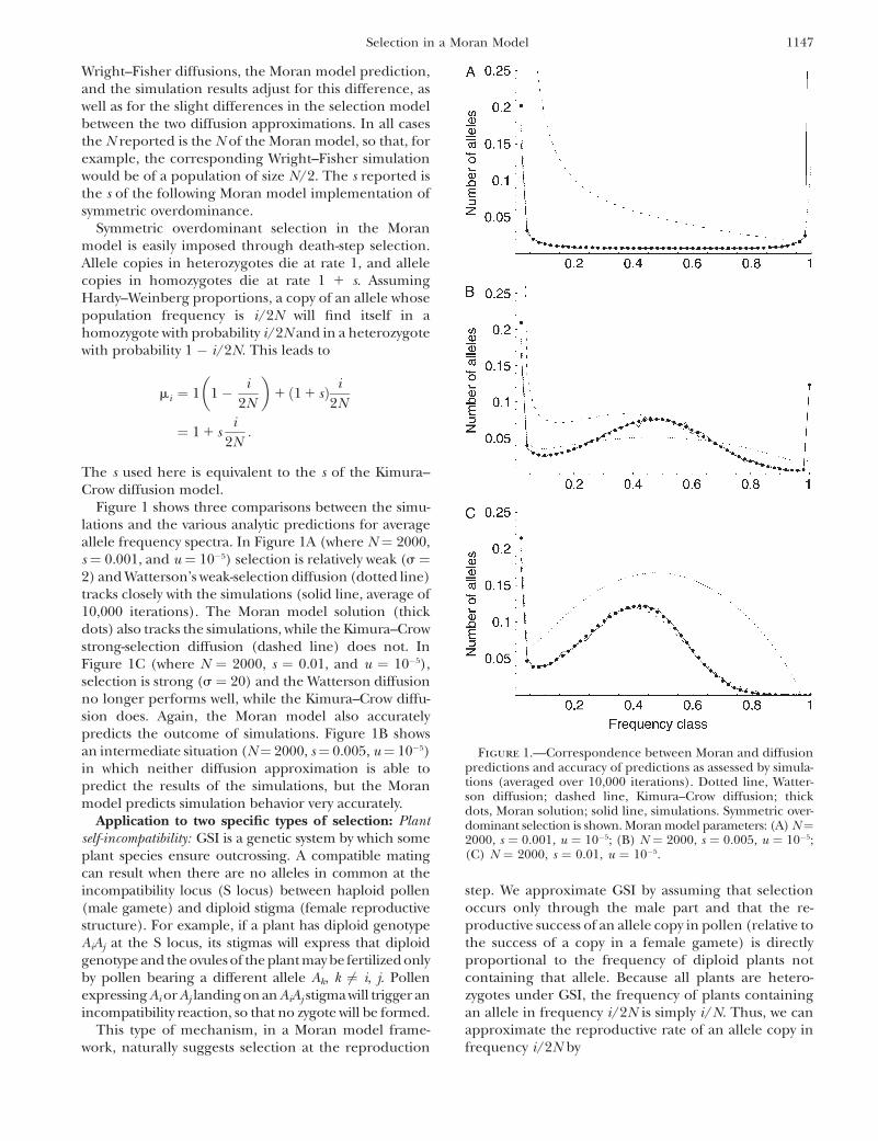
Figure 1 shows three comparisons between the simu-lations and the various analytic predictions for averageallele frequency spectra. In Figure 1A (where N ¼ 2000,s ¼ 0.001, and u ¼ 10�5) selection is relatively weak (s ¼2) and Watterson’s weak-selection diffusion (dotted line)tracks closely with the simulations (solid line, average of10,000 iterations). The Moran model solution (thickdots) also tracks the simulations, while the Kimura–Crowstrong-selection diffusion (dashed line) does not. InFigure 1C (where N ¼ 2000, s ¼ 0.01, and u ¼ 10�5),selection is strong (s ¼ 20) and the Watterson diffusionno longer performs well, while the Kimura–Crow diffu-sion does. Again, the Moran model also accuratelypredicts the outcome of simulations. Figure 1B showsan intermediate situation (N¼ 2000, s¼ 0.005, u¼ 10�5)in which neither diffusion approximation is able topredict the results of the simulations, but the Moranmodel predicts simulation behavior very accurately.

Application to two specific types of selection: Plantself-incompatibility: GSI is a genetic system by which someplant species ensure outcrossing. A compatible matingcan result when there are no alleles in common at theincompatibility locus (S locus) between haploid pollen(male gamete) and diploid stigma (female reproductivestructure). For example, if a plant has diploid genotypeAiAj at the S locus, its stigmas will express that diploidgenotype and the ovules of the plant may be fertilized onlyby pollen bearing a different allele Ak, k 6¼ i, j. Pollenexpressing Ai or Aj landing on an AiAj stigma will trigger anincompatibility reaction, so that no zygote will be formed.

This type of mechanism, in a Moran model frame-work, naturally suggests selection at the reproduction

step. We approximate GSI by assuming that selectionoccurs only through the male part and that the re-productive success of an allele copy in pollen (relative tothe success of a copy in a female gamete) is directlyproportional to the frequency of diploid plants notcontaining that allele. Because all plants are hetero-zygotes under GSI, the frequency of plants containingan allele in frequency i/2N is simply i/N. Thus, we canapproximate the reproductive rate of an allele copy infrequency i/2N by

Figure 1.—Correspondence between Moran and diffusionpredictions and accuracy of predictions as assessed by simula-tions (averaged over 10,000 iterations). Dotted line, Watter-son diffusion; dashed line, Kimura–Crow diffusion; thickdots, Moran solution; solid line, simulations. Symmetric over-dominant selection is shown. Moran model parameters: (A) N¼2000, s ¼ 0.001, u ¼ 10�5; (B) N ¼ 2000, s ¼ 0.005, u ¼ 10�5;(C) N ¼ 2000, s ¼ 0.01, u ¼ 10�5.


li ¼ 11

2

� �1 1� i

N

� �1

2

� �¼ 1� i

2N: ð14Þ

This approximation lacks some of the notable featuresof GSI. In particular, it does not require an overallnumber of alleles $3 (as required for a functional GSIsystem), and it does not restrict the allele frequencies tobe #0.5 (which follows directly from the observationthat all individuals in a GSI system must be hetero-zygotes). Nevertheless, this simple formulation per-forms well as judged by simulations.

The simulations shown in Figures 2 and 3 are again ofWright–Fisher (nonoverlapping generations) repro-duction with an appropriate population size conversionand in this case are individual-based simulations ofgametophytic plant self-incompatibility under an infin-ite-alleles model of mutation. GSI was simulated by thefollowing scheme: a diploid female parent and haploidpollen were picked randomly from the population andtested for compatibility. If they were compatible, a newzygote was generated from the possible gamete combi-nations; if incompatible, the pollen was discarded and anew pollen gamete picked until a compatible matingwas achieved. Mutation to novel alleles occurred withprobability u per gamete per generation.

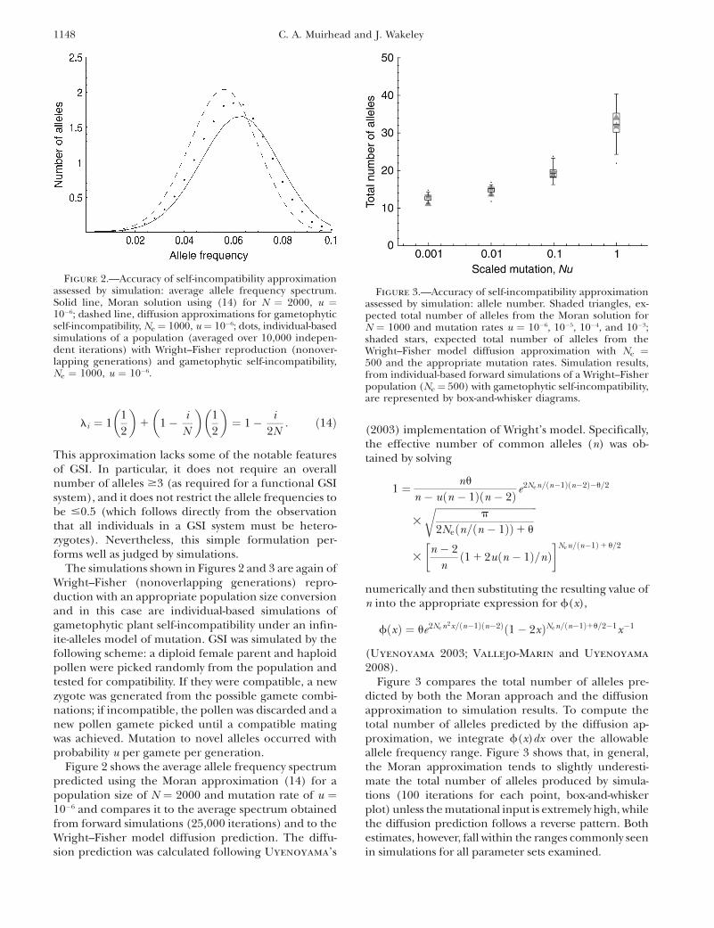
Figure 2 shows the average allele frequency spectrumpredicted using the Moran approximation (14) for apopulation size of N ¼ 2000 and mutation rate of u ¼10�6 and compares it to the average spectrum obtainedfrom forward simulations (25,000 iterations) and to theWright–Fisher model diffusion prediction. The diffu-sion prediction was calculated following Uyenoyama’s

(2003) implementation of Wright’s model. Specifically,the effective number of common alleles (n) was ob-tained by solving

1 ¼ nu

n � uðn � 1Þðn � 2Þ e2Nen=ðn�1Þðn�2Þ�u=2

3

ffiffiffiffiffiffiffiffiffiffiffiffiffiffiffiffiffiffiffiffiffiffiffiffiffiffiffiffiffiffiffiffiffiffiffiffiffiffiffiffiffip

2Neðn=ðn � 1ÞÞ1 u

r

3n � 2

nð1 1 2uðn � 1Þ=nÞ

� �Nen=ðn�1Þ1 u=2

numerically and then substituting the resulting value ofn into the appropriate expression for f(x),

fðxÞ ¼ ue2Nen2x=ðn�1Þðn�2Þð1� 2xÞNen=ðn�1Þ1u=2�1x�1

(Uyenoyama 2003; Vallejo-Marin and Uyenoyama

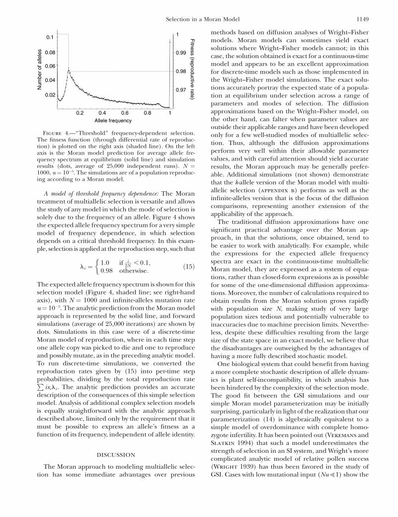
2008).Figure 3 compares the total number of alleles pre-

dicted by both the Moran approach and the diffusionapproximation to simulation results. To compute thetotal number of alleles predicted by the diffusion ap-proximation, we integrate f(x)dx over the allowableallele frequency range. Figure 3 shows that, in general,the Moran approximation tends to slightly underesti-mate the total number of alleles produced by simula-tions (100 iterations for each point, box-and-whiskerplot) unless the mutational input is extremely high, whilethe diffusion prediction follows a reverse pattern. Bothestimates, however, fall within the ranges commonly seenin simulations for all parameter sets examined.

Figure 2.—Accuracy of self-incompatibility approximationassessed by simulation: average allele frequency spectrum.Solid line, Moran solution using (14) for N ¼ 2000, u ¼10�6; dashed line, diffusion approximations for gametophyticself-incompatibility, Ne ¼ 1000, u¼ 10�6; dots, individual-basedsimulations of a population (averaged over 10,000 indepen-dent iterations) with Wright–Fisher reproduction (nonover-lapping generations) and gametophytic self-incompatibility,Ne ¼ 1000, u ¼ 10�6.

Figure 3.—Accuracy of self-incompatibility approximationassessed by simulation: allele number. Shaded triangles, ex-pected total number of alleles from the Moran solution forN ¼ 1000 and mutation rates u ¼ 10�6, 10�5, 10�4, and 10�3;shaded stars, expected total number of alleles from theWright–Fisher model diffusion approximation with Ne ¼500 and the appropriate mutation rates. Simulation results,from individual-based forward simulations of a Wright–Fisherpopulation (Ne¼ 500) with gametophytic self-incompatibility,are represented by box-and-whisker diagrams.


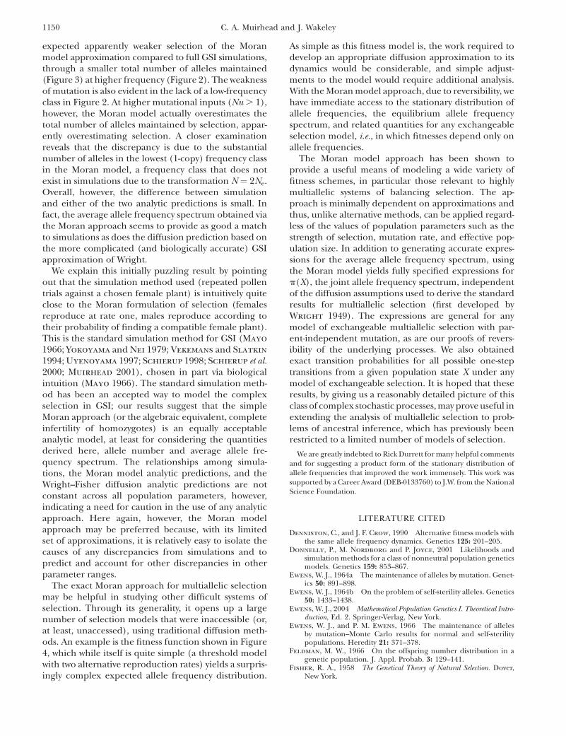
A model of threshold frequency dependence: The Morantreatment of multiallelic selection is versatile and allowsthe study of any model in which the mode of selection issolely due to the frequency of an allele. Figure 4 showsthe expected allele frequency spectrum for a very simplemodel of frequency dependence, in which selectiondepends on a critical threshold frequency. In this exam-ple, selection is applied at the reproduction step, such that

li ¼1:0 if i

2N , 0:1;0:98 otherwise:

�ð15Þ

The expected allele frequency spectrum is shown for thisselection model (Figure 4, shaded line; see right-handaxis), with N ¼ 1000 and infinite-alleles mutation rateu¼ 10�5. The analytic prediction from the Moran modelapproach is represented by the solid line, and forwardsimulations (average of 25,000 iterations) are shown bydots. Simulations in this case were of a discrete-timeMoran model of reproduction, where in each time stepone allele copy was picked to die and one to reproduceand possibly mutate, as in the preceding analytic model.To run discrete-time simulations, we converted thereproduction rates given by (15) into per-time stepprobabilities, dividing by the total reproduction rateP

ixili . The analytic prediction provides an accuratedescription of the consequences of this simple selectionmodel. Analysis of additional complex selection modelsis equally straightforward with the analytic approachdescribed above, limited only by the requirement that itmust be possible to express an allele’s fitness as afunction of its frequency, independent of allele identity.

DISCUSSION

The Moran approach to modeling multiallelic selec-tion has some immediate advantages over previous

methods based on diffusion analyses of Wright–Fishermodels. Moran models can sometimes yield exactsolutions where Wright–Fisher models cannot; in thiscase, the solution obtained is exact for a continuous-timemodel and appears to be an excellent approximationfor discrete-time models such as those implemented inthe Wright–Fisher model simulations. The exact solu-tions accurately portray the expected state of a popula-tion at equilibrium under selection across a range ofparameters and modes of selection. The diffusionapproximations based on the Wright–Fisher model, onthe other hand, can falter when parameter values areoutside their applicable ranges and have been developedonly for a few well-studied modes of multiallelic selec-tion. Thus, although the diffusion approximationsperform very well within their allowable parametervalues, and with careful attention should yield accurateresults, the Moran approach may be generally prefer-able. Additional simulations (not shown) demonstratethat the k-allele version of the Moran model with multi-allelic selection (appendix b) performs as well as theinfinite-alleles version that is the focus of the diffusioncomparisons, representing another extension of theapplicability of the approach.

The traditional diffusion approximations have onesignificant practical advantage over the Moran ap-proach, in that the solutions, once obtained, tend tobe easier to work with analytically. For example, whilethe expressions for the expected allele frequencyspectra are exact in the continuous-time multiallelicMoran model, they are expressed as a system of equa-tions, rather than closed-form expressions as is possiblefor some of the one-dimensional diffusion approxima-tions. Moreover, the number of calculations required toobtain results from the Moran solution grows rapidlywith population size N, making study of very largepopulation sizes tedious and potentially vulnerable toinaccuracies due to machine precision limits. Neverthe-less, despite these difficulties resulting from the largesize of the state space in an exact model, we believe thatthe disadvantages are outweighed by the advantages ofhaving a more fully described stochastic model.

One biological system that could benefit from havinga more complete stochastic description of allele dynam-ics is plant self-incompatibility, in which analysis hasbeen hindered by the complexity of the selection mode.The good fit between the GSI simulations and oursimple Moran model parameterization may be initiallysurprising, particularly in light of the realization that ourparameterization (14) is algebraically equivalent to asimple model of overdominance with complete homo-zygote infertility. It has been pointed out (Vekemans andSlatkin 1994) that such a model underestimates thestrength of selection in an SI system, and Wright’s morecomplicated analytic model of relative pollen success(Wright 1939) has thus been favored in the study ofGSI. Cases with low mutational input (Nu>1) show the

Figure 4.—‘‘Threshold’’ frequency-dependent selection.The fitness function (through differential rate of reproduc-tion) is plotted on the right axis (shaded line). On the leftaxis is the Moran model prediction for average allele fre-quency spectrum at equilibrium (solid line) and simulationresults (dots, average of 25,000 independent runs). N ¼1000, u¼ 10�5. The simulations are of a population reproduc-ing according to a Moran model.


expected apparently weaker selection of the Moranmodel approximation compared to full GSI simulations,through a smaller total number of alleles maintained(Figure 3) at higher frequency (Figure 2). The weaknessof mutation is also evident in the lack of a low-frequencyclass in Figure 2. At higher mutational inputs (Nu . 1),however, the Moran model actually overestimates thetotal number of alleles maintained by selection, appar-ently overestimating selection. A closer examinationreveals that the discrepancy is due to the substantialnumber of alleles in the lowest (1-copy) frequency classin the Moran model, a frequency class that does notexist in simulations due to the transformation N ¼ 2Ne.Overall, however, the difference between simulationand either of the two analytic predictions is small. Infact, the average allele frequency spectrum obtained viathe Moran approach seems to provide as good a matchto simulations as does the diffusion prediction based onthe more complicated (and biologically accurate) GSIapproximation of Wright.

We explain this initially puzzling result by pointingout that the simulation method used (repeated pollentrials against a chosen female plant) is intuitively quiteclose to the Moran formulation of selection (femalesreproduce at rate one, males reproduce according totheir probability of finding a compatible female plant).This is the standard simulation method for GSI (Mayo

1966; Yokoyama and Nei 1979; Vekemans and Slatkin

1994; Uyenoyama 1997; Schierup 1998; Schierup et al.2000; Muirhead 2001), chosen in part via biologicalintuition (Mayo 1966). The standard simulation meth-od has been an accepted way to model the complexselection in GSI; our results suggest that the simpleMoran approach (or the algebraic equivalent, completeinfertility of homozygotes) is an equally acceptableanalytic model, at least for considering the quantitiesderived here, allele number and average allele fre-quency spectrum. The relationships among simula-tions, the Moran model analytic predictions, and theWright–Fisher diffusion analytic predictions are notconstant across all population parameters, however,indicating a need for caution in the use of any analyticapproach. Here again, however, the Moran modelapproach may be preferred because, with its limitedset of approximations, it is relatively easy to isolate thecauses of any discrepancies from simulations and topredict and account for other discrepancies in otherparameter ranges.

The exact Moran approach for multiallelic selectionmay be helpful in studying other difficult systems ofselection. Through its generality, it opens up a largenumber of selection models that were inaccessible (or,at least, unaccessed), using traditional diffusion meth-ods. An example is the fitness function shown in Figure4, which while itself is quite simple (a threshold modelwith two alternative reproduction rates) yields a surpris-ingly complex expected allele frequency distribution.

As simple as this fitness model is, the work required todevelop an appropriate diffusion approximation to itsdynamics would be considerable, and simple adjust-ments to the model would require additional analysis.With the Moran model approach, due to reversibility, wehave immediate access to the stationary distribution ofallele frequencies, the equilibrium allele frequencyspectrum, and related quantities for any exchangeableselection model, i.e., in which fitnesses depend only onallele frequencies.

The Moran model approach has been shown toprovide a useful means of modeling a wide variety offitness schemes, in particular those relevant to highlymultiallelic systems of balancing selection. The ap-proach is minimally dependent on approximations andthus, unlike alternative methods, can be applied regard-less of the values of population parameters such as thestrength of selection, mutation rate, and effective pop-ulation size. In addition to generating accurate expres-sions for the average allele frequency spectrum, usingthe Moran model yields fully specified expressions forp(X), the joint allele frequency spectrum, independentof the diffusion assumptions used to derive the standardresults for multiallelic selection (first developed byWright 1949). The expressions are general for anymodel of exchangeable multiallelic selection with par-ent-independent mutation, as are our proofs of revers-ibility of the underlying processes. We also obtainedexact transition probabilities for all possible one-steptransitions from a given population state X under anymodel of exchangeable selection. It is hoped that theseresults, by giving us a reasonably detailed picture of thisclass of complex stochastic processes, may prove useful inextending the analysis of multiallelic selection to prob-lems of ancestral inference, which has previously beenrestricted to a limited number of models of selection.

We are greatly indebted to Rick Durrett for many helpful commentsand for suggesting a product form of the stationary distribution ofallele frequencies that improved the work immensely. This work wassupported by a Career Award (DEB-0133760) to J.W. from the NationalScience Foundation.

LITERATURE CITED

Denniston, C., and J. F. Crow, 1990 Alternative fitness models withthe same allele frequency dynamics. Genetics 125: 201–205.

Donnelly, P., M. Nordborg and P. Joyce, 2001 Likelihoods andsimulation methods for a class of nonneutral population geneticsmodels. Genetics 159: 853–867.

Ewens, W. J., 1964a The maintenance of alleles by mutation. Genet-ics 50: 891–898.

Ewens, W. J., 1964b On the problem of self-sterility alleles. Genetics50: 1433–1438.

Ewens, W. J., 2004 Mathematical Population Genetics I. Theoretical Intro-duction, Ed. 2. Springer-Verlag, New York.

Ewens, W. J., and P. M. Ewens, 1966 The maintenance of allelesby mutation–Monte Carlo results for normal and self-sterilitypopulations. Heredity 21: 371–378.

Feldman, M. W., 1966 On the offspring number distribution in agenetic population. J. Appl. Probab. 3: 129–141.

Fisher, R. A., 1958 The Genetical Theory of Natural Selection. Dover,New York.


Grote, M. N., and T. P. Speed, 2002 Approximate Ewens formulaefor symmetric overdominance selection. Ann. Appl. Probab. 12:637–663.

Hedrick, P. W., 2002 Pathogen resistance and genetic variation atMHC loci. Evolution 56: 1902–1908.

Ilmonen, P., D. Penn, K. Damjanovich, L. Morrison, L. Ghotbi

et al., 2007 Major histocompatibility complex heterozygosity re-duces fitness in experimentally infected mice. Genetics 176:2501–2508.

Kelly, F. P., 1979 Reversibility and Stochastic Networks. Wiley,Chichester, UK.

Kimura, M., and J. F. Crow, 1964 The number of alleles that can bemaintained in a finite population. Genetics 49: 725–738.

May, G., F. Shaw, H. Badrane and X. Vekemans, 1999 The signa-ture of balancing selection: fungal mating compatibility geneevolution. Proc. Natl. Acad. Sci. USA 96: 9172–9177.

Mayo, O., 1966 On the problem of self-incompatibility alleles. Bio-metrics 22: 111–120.

Moran, P. A. P., 1962 The Statistical Processes of Evolutionary Theory.Clarendon Press, Oxford.

Muirhead, C. A., 2001 Consequences of population structure ongenes under balancing selection. Evolution 55: 1532–1541.

Muirhead, C. A., N. L. Glass and M. Slatkin, 2002 Multilocus self-recognition systems in fungi as a cause of trans-species polymor-phism. Genetics 161: 633–641.

Paterson, S., K. Wilson and J. M. Pemberton, 1998 Major histo-compatibility complex variation associated with juvenile survivaland parasite resistance in a large unmanaged ungulate popula-tion (Ovis aries L.). Proc. Natl. Acad. Sci. USA 95: 3714–3719.

Penn, D. J., K. Damjanovich and W. K. Potts, 2002 MHC hetero-zygosity confers a selective advantage against multiple-strain in-fections. Proc. Natl. Acad. Sci. USA 99: 11260–11264.

Schierup, M. H., 1998 The number of self-incompatibility alleles ina finite, subdivided population. Genetics 149: 1153–1162.

Schierup, M. H., X. Vekemans and D. Charlesworth, 2000 Theeffect of subdivision on variation at multi-allelic loci under bal-ancing selection. Genet. Res. 76: 51–62.

Stephens, M., and P. Donnelly, 2003 Ancestral inference in popula-tion genetics models with selection. Aust. N. Z. J. Stat. 45: 395–430.

Stoffels, R. J., and H. G. Spencer, 2008 An asymmetric model ofheterozygote advantage at major histocompatibility complex

genes: degenerate pathogen recognition and intersection advan-tage. Genetics 178: 1473–1489.

Takahata, N., 1990 A simple genealogical structure of strongly bal-anced allelic lines and trans-species evolution of polymorphism.Proc. Natl. Acad. Sci. USA 87: 2419–2423.

Takahata, N., Y. Satta and Y. Klein, 1992 Polymorphism and bal-ancing selection at major histocompatibility complex loci. Genet-ics 130: 925–938.

Uyenoyama, M. K., 1997 Genealogical structure among alleles reg-ulating self-incompatibility in natural populations of floweringplants. Genetics 147: 1389–1400.

Uyenoyama, M. K., 2003 Genealogy-dependent variation in viabilityamong self-incompatibility genotypes. Theor. Popul. Biol. 63:281–293.

Vallejo-Marin, M., and M. K. Uyenoyama, 2008 On the Evolution-ary Modification of Self-Incompatibility: Implications of PartialClonality for Allelic Diversity and Genealogical Structure, pp.53–71 in Self-Incompatibility in Flowering Plants: Evolution, Diversity,and Mechanisms, edited by V. E. Franklin-tong. Springer-Verlag,Berlin/Heidelberg, Germany.

Vekemans, X., and M. Slatkin, 1994 Gene and allelic genealogiesat a gametophytic self-incompatibility locus. Genetics 137: 1157–1165.

Watterson, G. A., 1977 Heterosis or neutrality? Genetics 85: 789–814.

Wolfram, S., 2008 Mathematica, Version 7.0. Wolfram Research,Champaign, IL.

Wright, S., 1939 The distribution of self-sterility alleles in popula-tions. Genetics 24: 538–552.

Wright, S., 1949 Adaptation and Selection, pp. 365–389 in Genetics,Paleontology, and Evolution, edited by G. L. Jepsen, E. Mayr andG. G. Simpson. Princeton University Press, Princeton, NJ.

Wright, S., 1966 Polyallelic random drift in relation to evolution.Proc. Natl. Acad. Sci. USA 55: 1074–1081.

Yokoyama, S., and M. Nei, 1979 Population dynamics of sex-deter-mining alleles in honey bees and self-incompatibility alleles inplants. Genetics 91: 609–626.

Communicating editor: M. K. Uyenoyama

APPENDIX A: REVERSIBILITY, INFINITE-ALLELES MODEL

To simplify notation, let

ai ¼2Nu

1� u

1

m1

Yi

m¼2

m � 1

mmm

ðA1Þ

bi ¼2Nu

1� ul0

Yi

m¼2

ðm � 1Þlm�1

mðA2Þ

so that for our posited stationary distributions we have

pdðX Þ ¼ Cd

Y2N

i¼1

axii

xi !ðA3Þ

and

prðX Þ ¼ Cr

Y2N

i¼1

bxii

xi !: ðA4Þ

We begin by considering the selection at death stationary distribution. If the stationary distribution is correct, and theprocess is reversible, then


pdðX ÞqðX ;X 9Þ ¼ pdðX 9ÞqðX 9; X ÞpdðX ÞpdðX 9Þ ¼

qðX 9; X ÞqðX ; X 9Þ : ðA5Þ

Let ei be the unit vector with xi ¼ 1 and all other elements 0. From the transition types in Table 1, there are fourpossible detailed balances, with new population vectors X9 given by

X 9 ¼ X � ei�2 1 2ei�1 � ei ; i . 2;

X 9 ¼ X 1 ei�1 � ei � ej 1 ej11; i 6¼ 1; j 6¼ i; i � 1; i � 2;

X 9 ¼ X � e1 � ej 1 ej11; j 6¼ 1;

X 9 ¼ X � 2e1 1 e2:

To further simplify notation in evaluating the detailed balances, let fdðxiÞ ¼ axi

i =xi !. Then, for the first detailed balancein the selection at death model, we have

pdðX ÞpdðX 9Þ ¼

fdðxi�2Þfdðxi�2 � 1Þ

fdðxi�1Þfdðxi�1 1 2Þ

fdðxiÞfdðxi � 1Þ

¼ ai�2

xi�2

ðxi�1 1 1Þðxi�1 1 2Þa2

i�1

ai

xi

¼ mi�1ði � 1Þðxi�1 1 2Þði � 1Þðxi�1 1 1Þmi ixiði � 2Þxi�2

¼ qðX 9;X ÞqðX ;X 9Þ : ðA6Þ

The last line holds because this balance equation equates two events, ‘‘death of an i-copy allele and reproduction of an(i� 2)-copy allele (no mutation),’’ which has transition rate q(X, X9)¼miixi((i� 2)xi�2)(1� u), and ‘‘death of an (i� 1)-copy allele and reproduction of a different (i� 1)-copy allele (no mutation),’’ with rate q(X9, X)¼ mi�1(i� 1)(xi�1 1 2)((i � 1)(xi�1 1 1)/2N)(1 � u).

We have three remaining detailed balances to verify for the selection at death model. Substituting as before into(A5), we have for the second balance equation, for i 6¼ 1, and j 6¼ i, i � 1, i � 2, X9 ¼ X 1 ei�1 � ei � ej 1 ej11,




fdðxjÞfdðxj � 1Þ

fdðxj11Þfdðxj11 1 1Þ

¼ ðxi�1 1 1Þai�1

ai

xi

aj

xj

ðxj11 1 1Þaj11

¼mj11ð j 1 1Þðxj11 1 1Þði � 1Þðxi�1 1 1Þ

mi ixi jxj

¼ qðX 9;X ÞqðX ;X 9Þ ; ðA7Þ

where the two events are ‘‘i-copy dies, j-copy reproduces, no mutation,’’ with rate q(X, X9)¼ miixi( jxj/2N)(1 � u), and‘‘( j 1 1)-copy dies, (i� 1)-copy reproduces, no mutation,’’ with rate q(X9, X)¼mj11( j 1 1)(xj11 1 1)((i� 1)(xi�1 1 1)/2N)(1 � u).

The third balance uses, with X9 ¼ X � e1 � ej 1 ej11 and j 6¼ 1,



fdðx1Þfdðx1 � 1Þ



¼ a1

x1

aj

xj

xj11 1 1

aj11

¼mj11ð j 1 1Þðxj11 1 1Þ2Nu

m1x1jxjð1� uÞ

¼ qðX 9; X ÞqðX ; X 9Þ ; ðA8Þ

with the two events, ‘‘1-copy dies, j-copy reproduces, no mutation,’’ having rate q(X, X9) ¼ m1x1( jxj/2N)(1 � u), and‘‘( j 1 1)-copy dies, mutation,’’ with rate q(X9, X) ¼ mj11( j 1 1)(xj11 1 1)u.

The fourth detailed balance has X9 ¼ X � 2e1 1 e2, yielding


fdðx1Þfdðx1 � 2Þ

fdðx2Þfdðx2 1 1Þ

¼ a1

x1

a1

ðx1 � 1Þðx2 1 1Þ

a2

¼ m22ðx2 1 1Þ2Nu

m1x1ðx1 � 1Þð1� uÞ


where the two events are ‘‘1-copy dies, different 1-copy reproduces, no mutation,’’ with rate q(X, X9)¼ m1x1((x1� 1)/2N)(1 � u), and ‘‘2-copy dies, mutation,’’ with rate q(X9, X) ¼ m22(x2 1 1)u. And

prðX ÞqðX ; X 9Þ ¼ prðX 9ÞqðX 9; X Þ

prðX ÞprðX 9Þ ¼

qðX 9;X ÞqðX ;X 9Þ ðA10Þ

to verify the stationary distribution and reversibility of the process.For the first balance equation, we have for selection at reproduction,


frðxi�2Þfrðxi�2 � 1Þ

frðxi�1Þfrðxi�1 1 2Þ

frðxiÞfrðxi � 1Þ

¼ bi�2

xi�2

ðxi�1 1 1Þðxi�1 1 2Þb2

i�1

bi

xi

¼ ði � 1Þðxi�1 1 2Þli�1ði � 1Þðxi�1 1 1Þixili�2ði � 2Þxi�2

¼ qðX 9;X ÞqðX ;X 9Þ ðA11Þ

with q(X9, X) and q(X, X9) as before, with transition rates appropriate for selection at reproduction.For the second balance equation,




frðxjÞfrðxj � 1Þ

frðxj11Þfrðxj11 1 1Þ

¼ ðxi�1 1 1Þbi�1

bi

xi

bj

xj

ðxj11 1 1Þbj11

¼ ð j 1 1Þðxj11 1 1Þli�1ði � 1Þðxi�1 1 1Þixilj jxj

¼ qðX 9; X ÞqðX ; X 9Þ : ðA12Þ


The third balance equation gives


frðx1Þfrðx1 � 1Þ



¼ b1

x1

bj

xj

xj11 1 1

bj11

¼ ð j 1 1Þðxj11 1 1Þl02Nu

x1jlj xjð1� uÞ


and for the final detailed balance, we have


frðx1Þfrðx1 � 2Þ

frðx2Þfrðx2 1 1Þ

¼ b1

x1

b1

ðx1 � 1Þðx2 1 1Þ

b2

¼ 2ðx2 1 1Þl02Nu

x1l1ðx1 � 1Þð1� uÞ

¼ qðX 9; X ÞqðX ; X 9Þ : ðA14Þ

This completes the reversibility proof for the infinite-alleles model with selection at reproduction and validates theposited stationary distribution (2).

APPENDIX B: k-ALLELE MUTATION

Stationary distributions and reversibility: We now consider the case of k-allele mutation. In this model, there are kpossible allelic types, and the probability of mutation to a particular type is u/k, independent of the ‘‘parental’’ type, foreach reproduction event. Analysis of the k-allele model is similar to that of the infinite-alleles model, with some importantdepartures. The population state vector X now includes a term x0, representing the number of the k possible alleles notpresent in the population (i.e., those having zero copies). There are, as in the infinite-alleles models, 10 basic types oftransitions possible from a given X vector, but because of the different role of mutation, these transitions are not the sameas in the previous model. Because of the more consistent role of mutation in affecting alleles in different frequencyclasses, there are fewer special cases among the transitions that change the population state. We need to consider only twodetailed balances: one in which death and reproduction occur to copies in nonoverlapping frequency classes (affectingi, i� 1, j, and j 1 1, i 6¼ 0 and j 6¼ i, i� 1, i� 2) and one in which reproduction and death affect a common frequency class,similar to paired transitions 1 and 4 in the infinite-alleles model. Formally, the two X9 vectors we must consider are

X 9 ¼ X 1 ei�1 � ei � ej 1 ej11; i 6¼ 0; j 6¼ i; i � 1; i � 2

and

X 9 ¼ X � ei�2 1 2ei�1 � ei ; i . 1:

We again suggest expressions for the stationary distributions,

pkdðx0; x1; . . . ; x2N Þ ¼ Ckd

Y2N

i¼0

1

xi !

Yi

m¼1

ððm � 1Þ=2N Þð1� uÞ1 u=k

mmm

" #xi

ðB1Þ

for selection at death and

pkrðx0; x1; . . . ; x2N Þ ¼ Ckr

Y2N

i¼0

1

xi !

Yi

m¼1

lm�1ðððm � 1Þ=2N Þð1� uÞ1 u=kÞm

" #xi

ðB2Þ

for selection at reproduction, where Ckdand Ckr

again represent normalization constants. Reversibility can be verifiedby the same methods as before, using these stationary distributions and appropriate transition rates. Our simplifyingnotation is, for the k-allele model,


ai ¼Yi

m¼1

Rm�1

mmm

ðB3Þ

bi ¼Yi

m¼1

lm�1Rm�1

m; ðB4Þ

where we have defined Ri as

Ri ¼i

2Nð1� uÞ1 u

k: ðB5Þ

We also use fd(xi) and fr(xi) as before in the infinite-alleles model.For the first balance equation we have, with X9 ¼ X 1 ei�1 � ei � ej 1 ej11,

pkdðX ÞpkdðX 9Þ ¼





¼ ðxi�1 1 1Þai�1

ai

xi

aj

xj

ðxj11 1 1Þaj11

¼mj11ð j 1 1Þðxj11 1 1Þðxi�1 1 1ÞRi�1

mi ixixjRj

¼ qðX 9; X ÞqðX ; X 9Þ : ðB6Þ

Here the forward event is ‘‘an i-copy allele dies, and a new copy of a j-copy allele is created (through reproductionor mutation),’’ with rate q(X, X9) ¼ miixixjRj, and the reverse event is ‘‘a ( j 1 1)-copy allele dies, and a new copy of an(i � 1)-copy allele is created (through reproduction or mutation),’’ with rate q(X9, X) ¼ mj11(j 1 1)(xj11 1 1)(xi�1 1 1)Ri�1.

For the second balance, X9 ¼ X � ei�2 1 2ei�1 � ei, and with selection at death,

pkdðX ÞpkdðX 9Þ ¼

fdðxi�2Þfdðxi�2 � 1Þ



¼ ai�2

xi�2

ðxi�1 1 1Þðxi�1 1 2Þa2

i�1

ai

xi

¼ mi�1ði � 1Þðxi�1 1 2Þðxi�1 1 1ÞRi�1

mi ixixi�2Ri�2


The events here are ‘‘i-copy dies, and an (i � 2)-copy is created (through reproduction or mutation),’’ with rate q(X,X9) ¼ miixixi�2Ri�2, and ‘‘(i � 1)-copy dies, and a (different) (i � 1)-copy is created (through reproduction ormutation),’’ with rate q(X9, X) ¼ mi�1(i � 1)(xi�1 1 2)(xi�1 1 1)Ri�1.

This completes the reversibility proof for selection at death with k-allele mutation. The proof for the selection atreproduction case is similar, using the same balance equations. We have, for the first balance equation,

pkrðX ÞpkrðX 9Þ ¼





¼ ðxi�1 1 1Þbi�1

bi

xi

bj

xj

ðxj11 1 1Þbj11

¼ ð j 1 1Þðxj11 1 1Þli�1ðxi�1 1 1ÞRi�1

ixilj xjRj


For the second balance equation we have


pkrðX ÞpkrðX 9Þ ¼

frðxi�2Þfrðxi�2 � 1Þ



¼ bi�2

xi�2

ðxi�1 1 1Þðxi�1 1 2Þb2

i�1

bi

xi

¼ ði � 1Þðxi�1 1 2Þli�1ðxi�1 1 1ÞRi�1

ixili�2xi�2Ri�2

¼ qðX 9; X ÞqðX ; X 9Þ ; ðB9Þ

verifying the posited stationary distributions and reversibility in the Moran model of selection at reproduction under ak-allele model of mutation.

Average allele frequency spectra: To obtain the equilibrium expectations for X, we begin again with the identity (4),

E ½Xi � ¼X2N

j¼1

j

2NE ½XiXj �;

and focus on finding expressions for the cross-products E[XiXj]. Using the transitions in the first detailed balanceabove and taking expectations gives us, for the selection at death case,

mi iE ½XiXj �Rj ¼ mj11ð j 1 1ÞE ½Xj11Xi�1�Ri�1; i . 0; j 6¼ i; i � 1; i � 2

so that, for i , j

E ½XiXj � ¼j 1 1

i

mj11

mi

Ri�1

RjE ½Xi�1Xj11�: ðB10Þ

We also have from the other set of detailed balances that

mi iE ½XiðXi � 1Þ�Ri ¼ mi11ði 1 1ÞE ½Xi11Xi�1�Ri�1

for i . 1 or

E ½XiXi � ¼ E ½Xi �1i 1 1

i

mi11

mi

Ri�1

RiE ½Xi�1Xi11�: ðB11Þ

Combining (B10) and (B11), we have

E ½XiXj � ¼Yi

r¼1

j 1 r

i � r 1 1

mj1r

mi�r11

Ri�r

Rj1r�1

!E ½X0Xi1j �; i , j ðB12Þ

E ½XiXi � ¼ E ½Xi �1Yi

r¼1

i 1 r

i � r 1 1

mi1r

mi�r11

Ri�r

Ri1r�1

!E ½X0X2i �; ðB13Þ

leading to


j¼1

j

2N � i

Yj

r¼1

i 1 r

j � r 1 1

mi1r

mj�r11

Rj�r

Ri1r�1

!E ½X0Xi1j �

1X2N�i


j

2N � i

Yi

r¼1

j 1 r

i � r 1 1

mj1r

mi�r11

Ri�r

Rj1r�1

!E ½X0Xi1j �: ðB14Þ

These expressions are more complex than in the infinite-alleles case, and it appears that in addition to the problemof finding the set of 2N 1 1 E[Xi] elements, we have also set ourselves the task of first finding the set of E[X0Xi]elements. These tasks, however, can be accomplished simultaneously. We first note that


x0 ¼ k �X2N

j¼1

xj ;

and therefore

x0xi ¼ kxi �X2N

j¼1

xixj :

Then, taking the usual equilibrium expectations,

E ½X0Xi � ¼ kE ½Xi � �X2N

j¼1

E ½XiXj �: ðB15Þ

We then have

E ½X0Xi � ¼ ðk � 1ÞE ½Xi �

�XMinði;2N�iÞ

j¼1

Yj

r¼1

i 1 r

j � r 1 1

mi1r

mj�r11

Rj�r

Ri1r�1

!E ½X0Xi1j �

�X2N�i

Minði;2N�iÞ11

Yi

r¼1

j 1 r

i � r 1 1

mj1r

mi�r11

Ri�r

Rj1r�1


We have now expressed E[X0Xi] in terms of the ‘‘higher’’ vector elements E[X0Xi1j], just as we were able to expressE[Xi] in terms of the higher E[Xi1j] in the infinite-alleles model. In that case, we obtained results by calculating allE[Xi] terms beginning with E[X2N] and moving down the vector, relative to E[X2N], and then normalizing to obtainE[X2N]. Here, our procedure is very similar, but with an added layer of calculation as we move down the vector tocalculate the E[X0Xi]’s relative to E[X0X2N]. The procedure is straightforward because E[X0X2N]¼ (k� 1)E[X2N], andthus we can calculate all the E[X0Xi]’s, as well as E[Xi], relative to E[X2N], and normalize at the end as before. The fullexpression for E[Xi] obtained in this manner is cumbersome, but a computer program can calculate the values readily.As in the infinite-alleles model, once we have the expectations E[Xi], we can immediately calculate the normalizationconstant Ckd

, as well as Var[Xi] and Cov[XiXj] for the k-allele model.Analysis of k-allele mutation and reproduction-step selection is very similar, using the familiar balance equations and

the appropriate transition rates. The expression for the cross-product expectations in the case of selection atreproduction is

E ½XiXj � ¼Yi

r¼1

j 1 r

i � r 1 1

li�r

lj1r�1

Ri�r

Rj1r�1

!E ½X0Xi1j �; i , j ðB17Þ

E ½XiXi � ¼ E ½Xi �1Yi

r¼1

i 1 r

i � r 1 1

li�r

li1r�1

Ri�r

Ri1r�1

!E ½X0X2i � ðB18Þ

and we again use (B15) to obtain

E ½X0Xi � ¼ ðk � 1ÞE ½Xi �

�XMinði;2N�iÞ

j¼1

Yj

r¼1

i 1 r

j � r 1 1

lj�r

li1r�1

Rj�r

Ri1r�1

!E ½X0Xi1j �

�X2N�i

Minði;2N�iÞ

Yi

r¼1

j 1 r

i � r 1 1

li�r

lj1r�1

Ri�r

Rj1r�1


Again, a full expression for E[Xi] is not useful to write down, but a computer program can readily calculate the values.


Documents

Modeling Multiallelic Selection Using a ... - Wakeley Lab