Embed Size (px)
DESCRIPTION
Modeling Long Term Care and Supportive Housing. Marisela Mainegra Hing Telfer School of Management University of Ottawa. Canadian Operational Research Society, May 18, 2011. Outline. Long Term Care and Supportive Housing Queueing Models Dynamic Programming Model - PowerPoint PPT Presentation
Citation preview

Modeling Long Term Care and Supportive Housing
Marisela Mainegra Hing
Telfer School of Management
University of Ottawa
Canadian Operational Research Society, May 18, 2011

Outline
Long Term Care and Supportive Housing
Queueing Models
Dynamic Programming Model
Approximate Dynamic Programming

μLTC , CLTC
Community
Hospital
LTC
λC
λH
λRC
λRH
LTC problem
Goal:
Hospital level below a given threshold
Community waiting times below 90 days

LTC previous results
MDP model determined a threshold policy for the Hospital but it did not take into account community demands
Simulation Model determined that current capacity is insufficient to achieve the goal

Queueing Model
Station LTC: M/M/CLTC Station H_renege: M/M/∞
μLTC , CLTCλH-LTC
λC-LTC
λLTC
λRH
λRC
HospitalλH
Community λC
LTC
H_renege
μRH,

Queueing Model Station LTC: M/M/CLTC
LTCLTC
LTCLTC C
<1steady state:
1
1
00 !
/
!
/
LTC LTCC
c LTC
LTC
LTC
Cc
C
C
Ccp
02!1
/p
CCL
LTCLTC
C
qLTC
LTC
LTC
qLTCqLTC
LW
qLTCLTC
LTCHLTCqH LL
The probability that no patients are in the system:
The average number of patients in the waiting line:
The average time a client spends in the waiting line:
The number of patients from the Hospital that are in the queue for LTC (LqH-LTC).

Queueing Model Station H_renege: M/M/∞
The average number of patients in the system is
RH
RHRHL

Queueing Model Data analysis
Data on all hospital demand arriving to the CCAC from April 1st, 2006 to May 15th, 2009.
ρLTC = 1.6269 for current capacity CLTC= 4530
To have ρLTC < 1 we need CLTC> 7370.08, 2841 (62.71%) more beds than the current capacity.
With CLTC > 7370 we apply the formulas. Given a threshold T for the hospital patients and the
number LqLTC of total patients waiting to go to LTC, what we want is to determine the capacity CLTC in LTC such as:
LTCH
LTCRHqLTC LTL

Queueing Model Results
19 iterations of capacity values Goal achieved with capacity 7389, the
average waiting time is 31 days and the average amount of Hospital patients waiting in the queue is 130 ( T=134) .
This required capacity is 2859 (63.1%) more than the current capacity.

Queueing Model with SH
λRH
Hospital
μLTC , CLTC
λH-LTC
λRC
λH
Community λC
LTC
H_renege
λC-SH
λH-SH
SH
μSH , CSH
λSH-LTC
λC-LTC
μRH,

Queueing Model with SHResults
Required capacity in LTC is 6835, 2305 (50.883%) more beds than the current capacity (4530).
Required capacity in SH is 1169. With capacity values at LTC: 6835 and at SH:
1169 there are 133.9943 (T= 134) Hospital Patients waiting for care (for LTC: 110.3546, reneging: 22.7475, for SH: 0.89229), and Community Patients wait for care in average (days) at LTC: 34.8799, and at SH: 3.2433.

Semi-MDP ModelState space:
Action space:
Transition time:
Transition probabilities:
Immediate reward:
Optimal Criterion:
S = {(DH_LTC, DH_SH, DC_LTC, DC _SH, DSH_LTC, CLTC, CSH, p) }
A = {0,..,max(TCLTC,TCSH)}
d(s,a) =
Pr(s,a,s’) =
r(s,a) =
Total expected discounted reward
3p 1,
1,2p0,
3,)Pr()Pr(
2,1,15
1
2
1
pyx
p
i jji
3,
2,1,0
__
____ p
WTD
WTDTDD
p
LSHCSHC
LTCCLTCCCSHHLTCHH

Approximate Dynamic programming
'
0 00
( , )
'
(s,a) = E | ,
( , ) max , '
kTk
k
d s as'
as
Q r s s a a
r s a γ p Q (s' a )
γ: discount factor
find π : S A that maximizes the state-action value function
Goal
Bellman: there exists Q* optimal: Q* =maxQ(s,a) and the
optimal policy π* * *( ) arg max ( , )
as Q s a

stateaction
Reinforcement
Reinforcement Learning

RL: environment
transition probabilities
reward function
action
next state, immediate reward
ENVIROMMENT
state
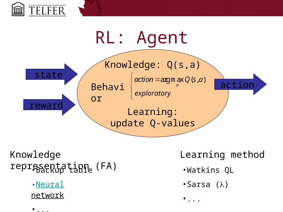
RL: Agent
Knowledge: Q(s,a)
exploratory
Learning:update Q-values
state
Knowledge representation (FA)
•Backup table
•Neural network
•...
•Watkins QL
•Sarsa ()
•...
reward
arg max ( , )a
action Q s aaction
Learning method
Behavior

QL: parameters θ: number of hidden neurons.
T: number of iterations of the learning process.
0: initial value of the learning rate.
0: initial value of the exploration rate.
Learning-rate decreasing function.
Exploration-rate decreasing function.Tt
Tt
t ..11
)( 0
Tt
Tt
t ..11
)( 0

QL: algorithm
exploration vs/ exploitation
Learning and exploration rates
θ(T,
T
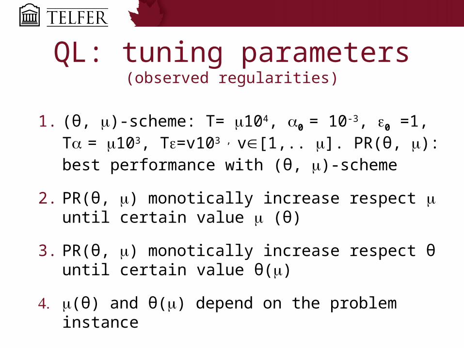
QL: tuning parameters(observed regularities)
1. (θ, )-scheme: T= 104, 0 = 10-3, 0 =1, T = 103, T=v103 , v[1,.. ]. PR(θ, ): best performance with (θ, )-scheme
2. PR(θ, ) monotically increase respect until certain value (θ)
3. PR(θ, ) monotically increase respect θ until certain value θ()
4. (θ) and θ() depend on the problem instance

QL: tuning parameters(methodology: learning schedule given PRHeu)
1. ∆θ =50, θ =0, PRθ =0, =0, vbest=1,
2. While PRθ <PRheu or no-stop
1. θ = θ + ∆θ, PRbest=0
2. While PRbest ≥ PR
1. = +1, T= 104, T = 103
2. PR=PRbest,
3. For v= vbest to • T=v103
• PR[v]=Q-Learning(T, θ, 10-3, 1, T , T)
4. [PRbest,vbest]=max(PR)
3. PRθ = PR

Discussion
For given capacities solve the SMDP with QL
Model other LTC complexities:• different facilities and room
accommodations, • client choice and • level of care

Thank you for your attention
Questions?

Neural Network for Q(s,a)
.
.
.
.
s
a
Q(s,a)
.
.