MODELING LOGGERHEAD TURTLE MOVEMENT IN THE … · Sea, and is applicable to other marine animal popula-tions that utilize highly dynamic and ephemerally distributed habitats. Our

Ecological Applications, 18(2), 2008, pp. 290–308� 2008 by the Ecological Society of America

MODELING LOGGERHEAD TURTLE MOVEMENT IN THEMEDITERRANEAN: IMPORTANCE OF BODY SIZE AND OCEANOGRAPHY

SCOTT A. ECKERT,1,2,5 JEFFREY E. MOORE,2 DANIEL C. DUNN,1,2,3 RICARDO SAGARMINAGA VAN BUITEN,4

KAREN L. ECKERT,1,2 AND PATRICK N. HALPIN2,3

1Wider Caribbean Sea Turtle Conservation Network (WIDECAST), Nicholas School of the Environment and Earth Sciences MarineLaboratory, Duke University, Beaufort, North Carolina 28516 USA

2Duke Center for Marine Conservation, Nicholas School of the Environment and Earth Sciences Marine Laboratory, Duke University,Beaufort, North Carolina 28516 USA

3Marine Geospatial Ecology Lab, Nicholas School of the Environment and Earth Sciences, Duke University,Durham, North Carolina 27708 USA

4Alnitak—Spanish Cetacean Society (SEC), Madrid, Spain

Abstract. Adapting state–space models (SSMs) to telemetry data has been helpful fordealing with location error and for modeling animal movements. We used a combination oftwo hierarchical Bayesian SSMs to estimate movement pathways from Argos satellite-tag datafor 15 juvenile loggerhead turtles (Caretta caretta) in the western Mediterranean Sea, and toprobabilistically assign locations to one of two behavioral movement types and relate thosebehaviors to environmental features. A Monte Carlo procedure helped propagate locationuncertainty from the first SSM into the estimation of behavioral states and environment–behavior relationships in the second SSM. Turtles using oceanic habitats of the Balearic Sea (n¼ 9 turtles) within the western Mediterranean were more likely to exhibit ‘‘intensive search’’behavior as might occur during foraging, but only larger turtles responded to variations in sea-surface height. This suggests that they were better able than smaller turtles to cue onenvironmental features that concentrate prey resources or were more dependent on high-quality feeding areas. These findings stress the importance of individual heterogeneity in theanalysis of movement behavior and, taken in concert with descriptive studies of Pacificloggerheads, suggest that directed movements toward patchy ephemeral resources may be ageneral property of larger juvenile loggerheads in different populations. We discovered size-based variation in loggerhead distribution and documented use of the western MediterraneanSea by turtles larger than previously thought to occur there. With one exception, onlyindividuals .57 cm curved carapace length used the most westerly basin in the Mediterranean(western Alboran Sea). These observations shed new light on loggerhead migration phenology.

Key words: Alboran Sea; animal movement; Caretta caretta; endangered species; environment–behaviorrelationships; hierarchical Bayes; juvenile loggerhead behavior; loggerhead sea turtle; Mediterranean Sea;oceanography; satellite telemetry; state–space model.

INTRODUCTION

Spatially explicit animal-movement models are in-

creasingly used to understand habitat selection (e.g.,

Arthur et al. 1996, Hjermann 2000, Fauchald and

Tveraa 2003, 2006, Morales et al. 2004, Preisler et al.

2004, Pinaud and Weimerskirch 2005, Breed et al. 2006,

Suryan et al. 2006). This is partly due to the difficulty in

meeting model assumptions of conventional selection

analyses that rely on a spatially implicit framework to

assess whether habitat use is nonrandom with respect to

the available habitat (Manly et al. 2002, Alldredge and

Griswold 2006). For example, many conventional

analyses require well-defined habitat categories within

well-defined use areas at individual or population levels.

However, both habitats and animal use areas are

difficult to define in many systems. In marine pelagic

systems, resource distributions are spatially and tempo-

rally dynamic or hierarchically structured (Valiela 1995,

Fauchald and Tveraa 2003, 2006, Pinaud and Weimer-

skirch 2005), and far-ranging migratory animals—such

as sea turtles—are not tied to central use areas for most

of the year (e.g., James et al. 2005, Eckert 2006, Polovina

et al. 2006). Conventional analyses also assume constant

habitat availability and independence of observed

animal locations. However, availability of habitat for

an individual may vary as a function of its current

location within large or undefined use-areas (Arthur et

al. 1996, Hjermann 2000, Rhodes et al. 2005), or because

the environment itself changes. Moreover, animal

locations from the same individual are rarely indepen-

dent, but rather, produce a complex, autocorrelated

time-series that may comprise multiple types of move-

ment behavior (Fauchald and Tveraa 2003, 2006,

Manuscript received 19 December 2006; revised 23 July 2007;accepted 24 July 2007; final version received 23 August 2007.Corresponding Editor: P. K. Dayton.

5 E-mail: [email protected]

290

Morales et al. 2004, Frair et al. 2005, Jonsen et al. 2005,

Sibert et al. 2006).

Spatial location error inherent to telemetry data poses

additional challenges for studying habitat selection. For

example, Argos satellite-telemetry data capture detailed

movement patterns of individuals over potentially long

time scales and large spatial regimes (Argos 2000), but

these data are recorded irregularly in time with varying

and sometimes large degrees of spatial error (Hays et al.

2001, Vincent et al. 2002, White and Sjoberg 2002).

Traditionally, locations known to contain extreme error

have been filtered using a priori criteria (Argos 2000,

Austin et al. 2003, Douglas 2006), and then analyses or

movement descriptions have been based on remaining

points. However, such filters may lead to information

loss, and at the same time ignore location error for

points that are not removed by the filter (Jonsen et al.

2005).

Adapting state–space models to location data has

been particularly helpful for modeling animal move-

ments while dealing with location error or temporal data

gaps (Anderson-Sprecher 1994, Sibert et al. 2003, 2006,

Morales et al. 2004, Jonsen et al. 2005, 2006, Royer et al.

2005, Nielsen et al. 2006). State–space models link two

types of equations: a transition equation, in which an

unobservable state variable (such as an animal’s true

location or behavioral state) changes through time

according to a Markov process, and an observation

equation that relates the state variable to the observed

data (e.g., locations recorded by telemetry methods, or

metrics characterizing successive movements). The goal

is to estimate the state variable. Applied to Argos (or

other telemetry) data, state–space models may be used

to estimate true animal locations at regular time

intervals (Jonsen et al. 2005, 2006, 2007). These improve

on a priori filters because no locations are discarded

(information loss is minimized), nor is location error

ignored for any point (Jonsen et al. 2005).

The Alboran Sea, extending from the Straits of

Gibraltar in the west to the Balearic Sea (Fig. 1), has

the highest biodiversity within the Mediterranean Sea

due to a combination of deep water and oceanic mixing

brought about by the flow of Atlantic Ocean waters

through the Straits (Tintore et al. 1988, Rodriguez et al.

1994, Send et. al. 1999). The region is an important

developmental area for thousands of juvenile and

subadult loggerhead sea turtles (Caretta caretta) that

originate from nesting areas in the western Atlantic and

eastern Mediterranean (Laurent et al. 1998, Carreras et

al. 2006) and congregate in pelagic habitats (Caminas

and de la Serna 1995, Caminas 1996, de Segura et al.

2006). This region also supports large fishing operations

that comprise a diverse array of gear types, including

longlines, driftnets, trawlers, and trammel nets, in which

FIG. 1. Map of the western Mediterranean Sea, including regional sea names and bathymetry.

March 2008 291STATE–SPACE MODELS OF SEA TURTLE MOVEMENT

thousands of juvenile loggerheads are incidentally

captured or killed annually (e.g., Aguilar et al. 1995,

Silvani et al. 1999, Carreras et al. 2004, Tudela et al.

2005). Given the endangered status of the Atlantic

loggerhead (IUCN 2006), reducing mortality of the

species in the western Mediterranean is vital to this

population’s conservation (Margaritoulis et al. 2003, de

Segura et al. 2006). While time–area fishing closures

might reduce loggerhead fishery interactions, little is

known about how juvenile loggerheads make use of

their environment in the region. Foraging habitats have

not been characterized, nor have movement patterns

been adequately explained in an oceanographic context.

Several studies have used Argos telemetry to examine

loggerhead movements in the Mediterranean, but these

have been primarily descriptive and have focused on

inter-nesting movements of adult females or migratory

patterns, not on movements of resident juveniles

(Caminas 1997, Bentivenga 2002, Hays et al. 2002,

Houghton et al. 2002, Godley et al. 2003). Cardona et al.

(2005) and Revelles et al. (2007) did investigate habitat

use and movements of juveniles in the western Mediter-

ranean on a finer temporal scale, and they defined

habitats on the basis of three bathymetric depth classes.

However they used conventional selection analyses,

which can be subject to the potential problems described

above, and they conducted their analyses separately for

individuals in their data set, which precluded the

evaluation of population-level patterns. Bentivenga et

al. (2007) investigated effects of currents on loggerhead

movement, but inference was limited by small sample

size and availability of data for currents. Such studies

have advanced our understanding of loggerhead move-

ments in the western Mediterranean, but there remains a

serious lack of knowledge about the linkage between

environmental features and the spatio-temporal distri-

butions of turtles.

More studies are needed—in this system and others—

that investigate habitat use in a spatially-explicit

analytical framework and that account for issues of

location error, and time-series data composed of

multiple behaviors, and that also address individual

variation in environment–behavior relationships (Thom-

as et al. 2006). Based on Argos satellite-tag data from 18

juvenile loggerheads captured in the western Mediterra-

nean, we first qualitatively evaluated large-scale rela-

tionships between turtle size and space use. Turtle size

corresponds to developmental stages characterized by

distinctive feeding and habitat ecologies (Bolten 2003).

Then, we used hierarchical Bayesian state–space models

to fit Mediterranean loggerhead pathways to the

satellite-tag data, and to probabilistically assign loca-

tions in the pathways, based on movement characteris-

tics, to one of two behavioral movement types that were

assumed to be dependent on environmental features and

turtle size class. Our work builds upon previous marine

state–space applications by modeling changes in animal

movement behavior explicitly as a function of dynamic

oceanographic variables within a hierarchical frame-

work and by addressing location uncertainty in evalu-ating environment–behavior relationships. We feel this

is an important step toward understanding habitatutilization of juvenile loggerheads in the Mediterranean

Sea, and is applicable to other marine animal popula-tions that utilize highly dynamic and ephemerallydistributed habitats. Our study yields novel and

important insights into the complex migration phenol-ogy of an endangered species.

METHODS

Capture and tagging of turtles

Between 6 July 2004 and 9 August 2005 juvenileloggerhead turtles were captured along a 520-km-long

section of the Spanish Mediterranean coast. Turtlesobserved at the surface were captured by hand by an

observer leaping from an inflatable boat. Turtles weretagged in the second scale of each front flipper with aninconel model 681s flipper tag (National Band and Tag

Company, Newport, Kentucky, USA), and a passiveintegrated transponder (PIT) tag (Avid Microchip ID

Systems, Folsom, Louisiana, USA) was inserted into thetriceps muscle. Turtles were measured (curved carapace

length and width), weighed, and scanned for internalfishing hooks with a metal detector (Zircon MT6;

Zircon, Campbell, California, USA). If a hook wasdetected, the turtle was released and was not involved in

the study.All turtles received a SDR-T16 or a SPOT4 platform

transmitter terminal (PTT) (Wildlife Computers, Red-mond, Washington, USA); these utilize the Argos

satellite telemetry system (Argos 2000) for data relayand location determination. Transmitters were mounted

to the highest part of the carapace, usually over thesecond vertebral (midline) scute (see Plate 1). The mount

area was cleaned with an abrasive plastic pad and wipedwith alcohol, and sanded lightly. The base of the PTT

was coated with a 1-cm-thick mixture of 45 mL ofA20/1000 high pressure borosilicate micro-balloons (3MCorporation, Saint Paul, Minnesota, USA) and 250 mL

of West Systems number 105 epoxy combined withnumber 205 hardener (West Systems, Watsonville,

California, USA). Use of the borosilicate micro-bal-loons thickened the resin and substantially reduced the

temperature of curing, thereby preventing damage to thecarapace and temperature-related discomfort to the

animal. Once the PTT was in place, a mixture of WestSystems number 105 epoxy and number 205 hardener

was used to apply fiberglass cloth over the transmitterand mount area. When the resin cured, the transmitter

and overlying resin were coated with dark blueantifouling paint (Interlux Micron 66; International

Paint, Union, New Jersey, USA).

State–space models

We used a combination of two state–space modelframeworks. In the first stage of analysis, we used the

SCOTT A. ECKERT ET AL.292 Ecological ApplicationsVol. 18, No. 2

framework developed by Jonsen et al. (2005) to

construct best-fit animal trajectories from Argos satellite

data. The state variable was a two-dimensional vector,

xt, representing the true locations of a turtle (longitude

and latitude) at regularly spaced intervals, t, while the

observed data, yt,i, consisted of locations recorded

irregularly in time from satellite tags (the subscript i

indexes multiple locations recorded during interval t). In

the second stage of our analysis, we used the framework

developed by Morales et al. (2004) to model switches in

movement behavior as a function of turtle size and

environmental covariates, which we sampled for each

estimated location xt (see Oceanographic sampling,

below). The state variable, bt, was a binary indicator

of behavioral state, with the transition expression

bt ; Bernoulliðpbt�1 ;ztÞ ð1Þ

where pbt�1;ztwas the probability of a turtle being in one

of two unobservable behavioral states during interval t,

and depended on the previous behavioral state (bt-1) and

environmental covariates (zt) sampled for location xt.

We tentatively interpret states 1 and 2 as intensive-

search or foraging vs. extensive-search or exploratory

states, respectively (e.g., Fauchald and Tveraa 2003,

2006, Morales et al. 2004). Thus,

p1;zt¼ expðztb1Þ

1þ expðztb1Þp2;zt¼ expðztb2Þ

1þ expðztb2Þð2Þ

expressed the probability of a turtle being in state 1 at t,

given that it was in state 1 or 2 at t � 1, respectively.

Parameter vectors for each state (b1, b2) were estimated

from the data.

There were two observation equations for this state–

space model: one for movement rates (dt; km/day) and

one for turn angles (ht; radians), calculated from the

locations (xt) estimated during the first modeling stage.

Data were viewed as random variables from distribu-

tions specific to each behavioral state. Following

Morales et al. (2004), we assumed that turn angles came

from wrapped Cauchy distributions, which are driven by

two parameters that must be estimated: the mean turn

angle (u) and the mean cosine of turn angles (x). Thedensity is

CðhÞ ¼ 1

2p1� x2

1þ x2 � 2xcosðh� uÞ

� �

0 � h � 2p 0 � x � 1: ð3Þ

For simplicity, and because we did not expect mean

turn angle to be systematically different for the two

behavioral states, we set mean turn angle (u) to zero.

Thus, we only needed to estimate x for each behavioral

state. In contrast to Morales et al. (2004), who used a

Weibull distribution for movement rate, we assumed

that movement rates for the two behavioral states came

from normal distributions with parameters l and r. Our

principal reason for using a normal distribution was to

always represent state 1 as the slower movement state

(l1 , l2). This constraint was easy to impose using the

normal, but was difficult with the Weibull distribution in

a hierarchical framework with multiple turtles. Move-

ment rates were not close to zero, so we were not

concerned that values from the normal distribution tails

would be underrepresented in the data. Thus, for a given

vector of behavioral states, the likelihood for our model

was

Pðdatajl;r;xÞ ¼YT

t¼1

Nðdtjlbt;rbtÞCðhtjxbt

Þ: ð4Þ

The ‘‘Jonsen method’’ also enables one to model

switches in movement behavior, based on estimates for

each behavioral state of mean turn angle and movement

correlation parameters (Jonsen et al. 2005, 2007).

However, we favored the ‘‘Morales method’’ because

we felt that its constituent parameters—mean movement

rate and variance in turn angles—offered a more

biologically intuitive characterization of different be-

havioral types for our study species, and that the latter

framework yielded a more believable separation of

movement types when applied to the same loggerhead

movement trajectory (see Supplement). Moreover, our

desire to explicitly model behavioral switching as a

function of environmental variables necessitated a two-

stage modeling process because we needed location

estimates from the Jonsen model before we could sample

oceanographic data. Once we had location estimates and

associated environmental data, the Morales framework

was more conducive to modeling environment–behavior

relationships. Jonsen et al. (2007) similarly evaluated the

relationship between environment and behavioral state

following output from their model that did not

incorporate environmental covariates.

Hierarchical Bayesian estimation

We implemented both modeling stages in a hierarchi-

cal Bayesian framework, which enabled us to explicitly

model individual heterogeneity in parameter estimates,

and to make efficient use of data from all turtles, even

those with few location data (e.g., Clark 2005, Jonsen et

al. 2006). Turtle size was included as a binary fixed

effect, with a value of 0 for turtles �46 cm curved

carapace length (CCL; ;40 cm straight carapace length

[SCL]) and 1 for turtles �53 cm CCL (our data set did

not include turtles between these values). This size break

corresponds to the suggested transitional size between

passive drifting and active habitat selection (Bolten

2003, Cardona et al. 2005). Random turtle effects were

incorporated by estimating hyper-parameters, which

describe population-level distributions and define the

prior distributions of individual-level parameters (see

Jonsen et al. [2006] for a flow chart of the hierarchical

model structure). Thus, individual-level parameters were

assumed to come from a normal (or in some cases beta)

population-level distribution, or hyper-distribution (Ta-

ble 1). We specified vague priors for hyper-distributions,


consistent with prior specifications of Morales et al.

(2004) and Jonsen et al. (2005, 2006). Some location

estimates (xt) did not have associated covariate estimates

because the oceanographic variables we sampled were

derived from satellite imagery whose quality is highly

dependent on the amount of cloud cover in the region.

We dealt with this by placing informative priors

(normal[0,1]) on the missing covariates (covariates were

standardized to normal[0,1] for analysis). We used

Monte Carlo Markov chain (MCMC) methods in

WinBUGS (version 1.4.1; Spiegelhalter et al. 2004) to

implement our models. For the Jonsen model, we

generated two MCMC chains, each with 20 000 itera-

tions. We discarded the first 15 000 samples from each

chain, and then thinned remaining observations by 10 to

reduce autocorrelation within the samples. For Morales-

based models, the chain length was 35 000. The first

10 000 were discarded and retained samples were

thinned by 50. Thus, posterior distributions for each

parameter were based on a total of 1000 independent

samples.

Oceanographic sampling

We examined the possible importance of bathymetric

depth, mean sea-level anomaly (MSLA), and the

interaction of MSLA with turtle size as predictors of

behavioral state. Previous analyses have shown that

juvenile loggerheads in the western Mediterranean are

generally associated with oceanic waters (.1400 m deep)

and seem to avoid waters of the continental shelf (,200

m; Cardona et al. 2005, Revelles et al. 2007). Polovina et

al. (2004, 2006) described associations between some

larger juvenile loggerheads and sea-surface heights,

indicative of features such as upwellings, downwellings,

or eddies that concentrate food resources (Rhines 2001,

Jacobs et al. 2002). We sampled these variables for all

locations along each turtle’s estimated trajectory. The

near real time (NRT) MSLA values (centimeters above

or below average sea-surface height for that location)

reflect ephemeral changes in surface height due to

upwellings, gyres, or cyclonic eddies: indicators of

surface productivity (Rhines 2001, Jacobs et al. 2002).

MSLA data, produced by SSALTO/DUACS (Issue

1rev5) and obtained from Aviso (available online),6 were

available as 3–4 day composites, and had a spatial

resolution of 0.25 degrees. We sampled bathymetric

depth (m) from the S2004 1-min global grid (Marks and

Smith 2006). This data set combines data from Smith

and Sandwell (1997) and the General Bathymetric Chart

of the Oceans (GEBCO) digital atlas (IOC, IHO, and

BODC 2003). It employs the GEBCO data for high

latitudes and longitudes, as well as in areas close to

shore, while maintaining the power of the short-

TABLE 1. Parameters and prior distributions for two stages of state–space modeling.

Parameter Prior distribution Interpretation

Stage-1 hyper-parmeters

hl uniform(�p, p) mean turn angle for populationhr uniform(0, 2) SD of turn angles, due to individual heterogeneitycl beta(1, 1) mean correlation in direction and turn angle between movesr half-norm(0, 1000) shape parameter for the beta distribution for ck (see below)s ¼ (r/cl) � r shape parameter for the beta distribution for ck (see below)

Stage-1 parameters

hk normalðhl; h2rÞ mean turn angle for turtle k

ck beta(r, s) mean correlation between movements for turtle kwk uniform(0, 10) a scaling factor that allows satellite tag error (Eq. 5) to vary for each turtleR Wishart covariance matrix for process variance (Eq. 3); same for all turtles

Stage-2 hyper-parameters

bl,b,i normal(0, 1000) mean coefficient for covariate i in state b; (i ¼ 0, 1, 2, 3, 4)br,b,i half-norm(0, 1000) SD of coefficients, due to individual heterogeneitydl,b half-norm(0, 1000) mean movement rate in state b, for populationdr,b half-norm(0, 1000) SD of movement rates in state b, due to individual heterogeneityd 00

l;b half-norm(0, 1000) mean variance in movement rate for state b, for population

d 00r;b half-norm(0, 1000) SD of variance in movement rate, due to individual heterogeneity

xl,b beta(1, 1) mean cosine of turn angles in state b, for populationr 0b half-norm (0, 1000) shape parameter for the beta distribution for xk,b (see below)s 0b ¼ ðr 0b=xl;bÞ � r 0b shape parameter for the beta distribution for xk,b (see below)

Stage-2 parameters

bk,b,i normalðbl;b;i; b2r;b;iÞ coefficient for covariate i, for turtle k in state b

dk,b normal(dl,b, dr,b2 ) mean movement rate of turtle k in state b

d 00k;b normalðd 00

l;b; d002r;bÞ SD of movement rate of turtle k in state b

xk,b betaðr 0b; s 0bÞ mean cosine of turn angles for turtle k in state b

Notes: See Jonsen et al. (2005) for explanation of stage-1 parameters; see Methods: State–space models and Morales et al. (2004)for explanation of stage-2 parameters; also see Supplement for code.

6 hhttp: / /www.aviso.oceanobs .com/html/donnees/produits/hauteurs/global/msla_uk.htmli


wavelength data in the Smith and Sandwell grid (Marks

and Smith 2006).

Propagating location uncertainty

Estimating behavioral states under the Morales (2004)

method assumes that animal locations, and hence rates

and turn angles, are measured without error. However,

location estimates from the Jonsen (2005) model are in

fact described by posterior distributions that reflect

location uncertainty. Because we believe that we should

account for uncertainty in rates and turn angles (a

function of location uncertainty) and location-specific

environmental data when estimating state probabilities

and effects of covariates, we conducted two sets of

analyses: an initial one that included 15 turtles and did

not address location uncertainty in estimating stage-2

model parameters, and a second analysis that included

only nine turtles and addressed location uncertainty in

stage-2 model estimates (see Results: Movement behavior

and oceanography: Analysis of 15 turtles . . . and Analysis

of nine turtles . . . , below). For the latter, we randomly

selected 30 turtle pathways (location estimates from 30

MCMC sample sets) from the posterior distributions of

location estimates from the stage-1 model. For each of

the 30 trajectory sets, we sampled oceanographic data

(depth and MSLA) and fit the stage-2 model. We

appended the 1000 samples from each of the 30 stage-2

outputs to obtain a final posterior distribution (30 000

total samples) for stage-2 parameter estimates.

RESULTS

Description of turtles and movement paths

Nineteen juvenile loggerhead turtles (Caretta caretta)

were captured, with sizes ranging from 26 to 79 cm curved

carapace length (CCL; 57.0 6 18.9 cm [mean 6 SD]) and

from 2.8 to 60.0 kg (32.6 6 21.5 kg [mean 6 SD]) (Table

2). Capture longitude and turtle sizes were significantly

correlated (Pearson r¼ 0.56, P , 0.05), with larger turtles

being caught further west (Table 2). Ten of the 11 turtles

with CCL .57.0 cm (Table 2) were captured west of 38W

corresponding roughly to the eastern edge of the Alboran

basin. All but one turtle (Cc17) with CCL �57 cm (n¼ 8

turtles) were captured east of 38W (Table 2). There was no

relation between month of capture and turtle size

(Pearson r¼ 0.13, P . 0.05). One turtle (Cc5) transmitted

satellite data for only one day and was not considered in

further analysis or interpretation. Monitoring duration of

the remaining 18 turtles spanned 7–562 days (150.1 6

142.4 days [mean 6 SD]; Table 2).

Of the 18 turtles with monitoring durations �7 days,

post-capture movements exhibited two general patterns

that seemed related to turtle size. Turtles with CCL

�57cm (n ¼ 8) (Cc8, Cc10, Cc11, Cc12, Cc13, Cc14,Cc15, and Cc17) gradually moved eastward through the

Mediterranean Sea after capture (Fig. 2). Six (Cc8,

Cc10, Cc13, Cc14, Cc15, and Cc17) of these eight

smaller turtles spent most of their time in southern

Balearic Sea (western Mediterranean basin); the other

two small turtles (Cc11 and Cc12) moved along the

Moroccan and Algerian coasts, apparently with the

Algerian current, to more easterly basins. Turtle Cc11

moved into the Ionian Sea. Turtle Cc12 moved into the

Tyrrhenian Sea before traveling north to the south coast

of France and west along the Spanish coast (Fig. 2). The

10 turtles with CCL .57 cm displayed more variation in

movement patterns. Three (Cc1, Cc3, and Cc4; Fig. 3)

moved east across the Mediterranean in a manner

similar to the smaller turtles, whereas seven (Cc2, Cc6,

TABLE 2. Information on 19 loggerhead sea turtles (Caretta caretta) and satellite transmitters deployed on these turtles in thewestern Mediterranean Sea.

TurtleID

Size,CCL

Mass(kg)

Deploymentdate

Lasttransmission

No. daysmonitored

Transmittermodel

Deploymentlongitude (8W)

Cc1 74.0 57.50 6 Jul 2004 12 May 2005 311 SDR-T16 5.44Cc2 68.0 47.00 11 Jul 2004 30 Jul 2004 19 SDR-T16 5.19Cc3 69.0 35.70 12 Jul 2004 14 Dec 2004 155 SDR-T16 5.17Cc4 79.0 60.00 18 Jul 2004 3 Dec 2004 138 SPOT 4 4.87Cc5� 60.5 31.60 19 Jul 2004 20 Jul 2004 1 SDR-T16 5.21Cc6� 76.0 54.65 20 Jul 2004 28 Nov 2004 131 SDR-T16 5.22Cc7� 76.0 55.00 22 Jul 2004 21 Dec 2004 152 SPOT 4 4.89Cc8 30.0 4.50 20 Sep 2004 27 Mar 2005 188 SPOT 4 1.42Cc9 71.0 40.00 10 Oct 2004 16 Oct 2004 7 SPOT 4 1.04Cc10 32.0 5.80 13 Oct 2004 1 Nov 2004 19 SPOT 4 0.53Cc11 26.0 2.80 24 Nov 2004 15 Mar 2005 111 SPOT 4 2.50Cc12 53.0 NA 4 Dec 2004 18 Jun 2006 562 SPOT 4 1.04Cc13 57.0 22.00 24 Jan 2005 13 Aug 2005 201 SPOT 4 2.93Cc14 44.0 12.80 20 Mar 2005 16 May 2005 57 SPOT 4 2.00Cc15 46.0 14.20 20 Mar 2005 9 Jul 2005 154 SPOT 4 2.00Cc16 68.0 48.00 7 Jul 2005 21 Aug 2005 46 SPOT 4 4.55Cc17 28.0 3.40 7 Jul 2005 30 Jul 2005 23 SPOT 4 4.58Cc18� 74.0 54.00 12 Jul 2005 10 Jul 2006 363 SPOT 4 4.27Cc19 77.0 54.00 9 Aug 2005 15 Oct 2005 67 SPOT 4 2.80

Note: Key to abbreviations: CCL ¼ curved carapace length; NA ¼ not available (turtle was not weighed).� Four turtles were not used in state–space model analysis because they only transmitted location data for one day (Cc5) or left

the Mediterranean and traveled across the Atlantic Ocean (Cc6, Cc7, and Cc18).


Cc7, Cc9, Cc16, Cc 18, and Cc19) were associated with

waters of the Alboran Sea (see Plate 1). Three of these

seven (Cc6, Cc7, and Cc18) left the Mediterranean and

moved west across the Atlantic Ocean (Fig. 4). In the

longest and most complete of these trans-Atlantic

records (Cc18), the turtle traveled to the southern coast

of Nicaragua in the Caribbean Sea (Fig. 4). Turtles Cc6

and Cc7 appeared to be moving toward the Caribbean

and United States coast, respectively, before we stopped

receiving transmissions.

Movement behavior and oceanography

The 15 turtles that remained in the Mediterranean Sea

were considered for our state–space models. A total of

FIG. 2. Fitted trajectories from state–space models, based on Argos satellite telemetry data, of eight juvenile loggerhead seaturtles �57 cm CCL, captured in the southern Balearic Sea. The shaded circles at the west end of the trajectory indicate capturelocation. The dotted line for Cc12 represents a 37-day period (20 January–26 February 2006) during which no location data wererecorded for this turtle.


5472 Argos-recorded locations from these turtles were

entered into our analyses. At the time of this analysis the

number of locations per turtle ranged from 38 to 728

locations (median: 359 locations). The locations spanned

a total of 1861 intervals or ‘‘turtle-days,’’ with the

number of days per turtle ranging from 7 to 410 days

(median: 110 days). Stage-1 state–space models (see

Supplement for parameter estimates) improved on

unprocessed telemetry data by removing extreme loca-

tions and estimating more accurate trajectories than

provided by unprocessed satellite tag data (Fig. 5).

Analysis of 15 turtles in the western Mediterranean.—

We first describe population-level parameter estimates

(hyper-parameters), based on the model that included 15

turtles and assumed that location estimates from the

Jonsen model were error free. Mean movement rate of

turtles in state 1 (intensive search) was 13.6 km/day

(95% crecible interval [CI]: 11.3–17.3 km), with an SD of

FIG. 3. Fitted trajectories from state–space models, based on Argos satellite telemetry data, of juvenile and subadult loggerheadsea turtles .57 cm CCL captured in the Alboran and Balearic Seas (western Mediterranean Sea) as monitored using Argos satellitetelemetry. Circles indicate capture location.


4.0 km (2.3–8.5 km) across individuals, compared to

37.8 km (31.4–43.8 km) with a SD of 10.2 km (6.9–15.6

km) across turtles in state 2 (exploratory). The wrapped

Cauchy parameter, x, reflects the amount of variance in

turn angles, with smaller values reflecting more tortuous

movement. Median x for state 1 (xl,1) was 0.37 (95%

CI: 0.28–0.46) compared to 0.44 (0.34–0.57) for state 2

(xl,2), which at first seems to suggest that movement

tortuousity in slow (state 1) and fast (state 2) movement

states was similar. However, tortuousity of state-2

movement varied considerably across individuals (xr,2

¼ 0.30; Fig. 6). For seven turtles (Cc1, Cc3, Cc8, Cc11,

Cc12, Cc13, and Cc14)—all of whom traveled east

through the Mediterranean following capture (Figs. 2

and 3)—the slower state was also more tortuous, as

evidenced by non- or only slightly overlapping 95%

credible intervals for the parameters xk,1 and xk,2 (Figs.

5A and 6). The opposite was true for four large turtles

that used the Alboran (Cc2, Cc4, Cc16, and Cc19; Fig.

3); the faster state was highly tortuous for these turtles

(Figs. 5B and 6). For four turtles (Cc9, Cc10, Cc15, and

Cc17; Figs. 2 and 3), movement tortuousity was

statistically similar for the two states (Fig. 6), but three

of these turtles (Cc9, Cc10, and Cc17) had few location

data (n¼ 7, 19, and 23 days, respectively; Table 2), and

point estimates for all four of these turtles suggested

greater tortuousity in state 1. Thus, it appeared that

state 1 (slower state) was typically more tortuous for

turtles using oceanic waters east of the Alboran, and

that movement characteristics outside of the Alboran

Sea were distinctly different from movement within the

shallower Alboran basins. The degree of certainty in

assigning movement segments to one of the two

behavioral states was generally high, with median

Prob(state 1) usually .0.75 or ,0.25 (indicating state

2) (Fig. 5).

Coefficients describing effects of environmental fea-

tures and turtle size on behavioral switching suggested

that all covariates included in our model were important

predictors of behavioral state. First, juvenile logger-

heads were more likely to exhibit the slower state 1

(intensive search) movement when in deeper waters.

Standardized hyper-parameters (denoted by subscript l)for depth (subscript D), with subscript 1 or 2 indicating

switching to state 1 from either respective state, were:

bl,1,D¼�0.71 (95% Bayesian CI¼ [�1.51,�0.13]; Prob[b, 0] ¼ 0.99); bl,2,D ¼ �0.37 (95% CI ¼ [�1.22, 0.13];Prob[b , 0] ¼ 0.94). Individual-level responses were

generally consistent with this population-level result

(Fig. 7). Second, juveniles of the larger size class showed

more persistent bouts of ‘‘fast’’ swimming behavior, i.e.,

a larger turtle exhibiting state-2 movement was more

FIG. 4. Tracklines of three subadult loggerhead sea turtles as monitored using Argos satellite telemetry and processed using aDouglas filter (Douglas 2006). Turtles were captured in the Alboran Sea (western Mediterranean) and monitored for up to 363 daysas they moved west across the Atlantic Ocean. The circles in the inset indicate capture location. Shading reflects bathymetry as inFig. 1.


likely to remain in that state than was a smaller turtle.

Standardized coefficients for turtle size (subscript S)

were: b1,S¼�0.21 (95% CI: [�1.37, 1.15]; Prob[b , 0]¼0.64); b2,S¼�0.99 (95% CI: [�2.54, 0.14]; Prob[b , 0]¼0.95). Finally, larger juveniles seemed to respond

behaviorally to MSLA, with lower MSLA values

increasing the probability of switching from fast (state

2) to slow (state 1) movement. Standardized hyper-

parameters describing the effect of MSLA for larger

juveniles (subscript Ml) (i.e., bl,i,Ml ¼ bl,i,M þ bl,i,S3M,

when size class¼ 1) were: bl,1,Ml¼�0.15 (95% Bayesian

CI ¼ [�0.92, 0.68]; Prob[b , 0] ¼ 0.65); bl,2,Ml ¼�0.56(95% CI ¼ [�1.58, 0.07]; Prob[b , 0] ¼ 0.96). Median

and 95% credible estimates for the size 3 MSLA

interaction (S3M subscript) terms themselves were:

bl,1,S3M ¼ �0.38 (95% Bayesian CI ¼ [�1.82, 0.86];

Prob[b , 0]¼ 0.76); bl,2,S3M¼�1.32 (95% CI¼ [�3.18,0.11]; Prob[b , 0] ¼ 0.97). Smaller individuals did not

seem to respond behaviorally to MSLA, with 28% and

12% of the posterior densities for bl,1,M (b¼ 0.26 [�0.64,1.46]) and bl,2,M (b ¼ 0.74 [�0.61, 2.26]) overlapping

zero. After accounting for the role of turtle size, there

did not appear to be any strong unique individual-level

responses to MSLA (Fig. 7).

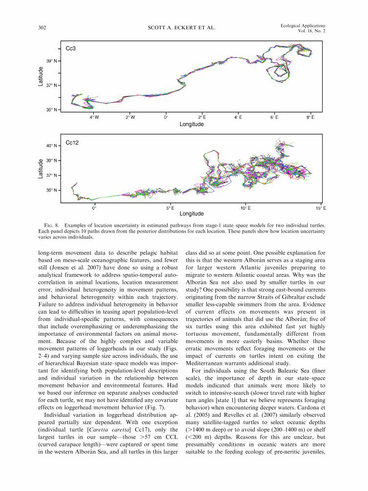
Analysis of nine turtles in the Balearic Sea.—Our first

set of results suggested that it may not be appropriate to

model movements in the Alboran Sea, Balearic Sea, and

basins east of the Balearics as a single statistical

population, since turtles using these areas displayed

different types of movement. Therefore, we fit a separate

stage-2 hierarchical model to the nine turtles that spent

the majority of time in the southern Balearic Sea and did

not move to more easterly basins (Cc1, Cc3, Cc4, Cc8,

Cc10, Cc13, Cc14, Cc15, and Cc17; Figs. 2 and 3). This

second set of analyses incorporated location uncertainty

from the stage-1 Jonsen model, which varied consider-

ably across turtles (Fig. 8), into stage-2 parameter

estimation. Results were qualitatively similar to the

analysis that included all 15 turtles, but with some

noteworthy differences. Hyper-parameter estimates for

mean movement rates were 16.0 (95% CI: 13.2–18.8) and

36.3 km/day (31.6–41.9), for states 1 and 2, respectively.

These are similar to the first set of analyses; however

variation across individuals was much lower in the

second analysis, with a SD for the hyper-distribution of

2.9 km/day (1.1–5.5) and 3.1 km/day (1.5–7.2), respec-

tively. Also, state 1 (slower) movement was definitively

more tortuous in the newer model (hyper-parameters:

xl,1¼ 0.18 [95% CI: 0.09–0.30]; xl,2¼ 0.44 [0.30–0.58]),

and tortuousity for state 2 also was less variable across

individuals than in the previous model (Fig. 9). The

exception to this was turtle Cc4, a large turtle (CCL¼79

cm), for which the faster mode was more tortuous. As in

the first analysis, this contrasting result may be

explained by fast tortuous movement displayed by Cc4

in the western Alboran Sea before it traveled into the

southern Balearic Sea (Fig. 3).

As in the first analysis, loggerheads in the southern

Balearic Sea were more likely to exhibit intensive search

behavior in deeper oceanic waters, as indicated by high

probability that bl,1,D and bl,2,D differed from 0 (Table

3; also see Fig. 10). Also consistent with the first

analysis, larger individuals seemed to respond behav-

iorally to MSLA. Standardized hyper-parameters de-

scribing the effect of MSLA for larger juveniles (i.e.,

bl,i,Ml¼ bl,i,M þ bl,i,S3M, when size class¼ 1) suggested

that the probability of bl,2,Ml being ,0 was 0.97 (Table

3). Thus, lower MSLA values increased the probability

of switching from fast (state 2) to slow (state 1)

movement (Fig. 10A), but did not affect the probability

FIG. 5. Examples of using state–space models to fitmovement trajectories to Argos data for juvenile loggerheadsea turtles in the western Mediterranean Sea. Gray lines andopen circles depict location data from the Argos satellitesystem. Solid symbols depict estimated locations (at 1-dayintervals) from stage-1 state–space models fit to the satellite-tagdata, and estimated behaviors (uncertain, if Prob(state 1) is.0.25 and ,0.75) based on the stage-2 state–space model.


of staying in state 1 if already in that state. MSLA was

not associated with behavioral switch probability for

small individuals, with 16% and 31% of the posterior

densities for bl,1,M and bl,2,M overlapping 0 (Table 3).

Unlike the first-analysis results, size alone was not a

strong predictor of behavioral state; larger juvenile

turtles within the southern Balearic Sea did not

conclusively display more persistent state-2 movement

than smaller turtles (Prob[b1,S] , 0.32; Prob[b2,S , 0]¼

0.83). As with the first analysis, there did not appear to

be any unique individual responses to MSLA or depth

apart from size-related responses to MSLA.

Importance of propagating location uncertainty

For comparison, we repeated our analysis for the nine

turtles that used the southern Balearic Sea, but we

treated location estimates from the stage-1 state–space

model as error-free in the second stage of modeling (i.e.,

FIG. 6. Medians and 95% Bayesian credible intervals for standardized random-effect parameters describing mean movementrate and movement tortuosity to indicate the variance of turn angles (unitless, between 0 and 1; a wrapped Cauchy parameter, seeMethods: State–space models) of two behavioral states, based on a stage-2 state–space model fitted to pathways of 15 juvenileloggerheads in the western Mediterranean Sea. Pathways estimated from the stage-1 state–space model were assumed to havenegligible location error.


this was like our analysis of 15 turtles). This had minor

but nontrivial impacts on our inference. Bayesian

credible intervals for stage-2 parameters were wider

when location uncertainty was addressed (Table 3), with

consequences for interpreting the predictive importance

of different parameters. For example, if we had ignored

location uncertainty in our second analysis, we would

have concluded a stronger effect of turtle size on the

probability of switching from state 2 to state 1 (i.e.,

Prob[b , 0] ¼ 0.93 when location uncertainty was

ignored vs. 0.83 when location uncertainty was propa-

gated). Similarly, we may have inferred a meaningful

impact of MSLA on behavioral switching in small

turtles (which would have appeared opposite to that of

large turtles) if location uncertainty was ignored.

DISCUSSION

Size-dependent variation in distribution and movement

Globally and across sea turtle species, few studies

(Ferraroli et al. 2004, Polovina et al. 2004, 2006,

Cardona et al. 2005, Revelles et al. 2007) have used

FIG. 7. Medians and 95% Bayesian credible intervals for standardized random-effect parameters describing the influence of depthand mean sea-level anomaly (MSLA) on behavioral switching by individual (k) juvenile loggerheads, based on a stage-2 state–spacemodel fitted to pathways of 15 turtles in the western Mediterranean Sea. Pathways were estimated from the stage-1 state–space modeland were assumed to have negligible location error. Parameters indicate the effect of the variable on switching to state 1 from state i.


long-term movement data to describe pelagic habitat

based on meso-scale oceanographic features, and fewer

still (Jonsen et al. 2007) have done so using a robust

analytical framework to address spatio-temporal auto-

correlation in animal locations, location measurement

error, individual heterogeneity in movement patterns,

and behavioral heterogeneity within each trajectory.

Failure to address individual heterogeneity in behavior

can lead to difficulties in teasing apart population-level

from individual-specific patterns, with consequences

that include overemphasizing or underemphasizing the

importance of environmental factors on animal move-

ment. Because of the highly complex and variable

movement patterns of loggerheads in our study (Figs.

2–4) and varying sample size across individuals, the use

of hierarchical Bayesian state–space models was impor-

tant for identifying both population-level descriptions

and individual variation in the relationship between

movement behavior and environmental features. Had

we based our inference on separate analyses conducted

for each turtle, we may not have identified any covariate

effects on loggerhead movement behavior (Fig. 7).

Individual variation in loggerhead distribution ap-

peared partially size dependent. With one exception

(individual turtle [Caretta caretta] Cc17), only the

largest turtles in our sample—those .57 cm CCL

(curved carapace length)—were captured or spent time

in the western Alboran Sea, and all turtles in this larger

class did so at some point. One possible explanation for

this is that the western Alboran serves as a staging area

for larger western Atlantic juveniles preparing to

migrate to western Atlantic coastal areas. Why was the

Alboran Sea not also used by smaller turtles in our

study? One possibility is that strong east-bound currents

originating from the narrow Straits of Gibraltar exclude

smaller less-capable swimmers from the area. Evidence

of current effects on movements was present in

trajectories of animals that did use the Alboran; five of

six turtles using this area exhibited fast yet highly

tortuous movement, fundamentally different from

movements in more easterly basins. Whether these

erratic movements reflect foraging movements or the

impact of currents on turtles intent on exiting the

Mediterranean warrants additional study.

For individuals using the South Balearic Sea (finer

scale), the importance of depth in our state–space

models indicated that animals were more likely to

switch to intensive-search (slower travel rate with higher

turn angles [state 1] that we believe represents foraging

behavior) when encountering deeper waters. Cardona et

al. (2005) and Revelles et al. (2007) similarly observed

many satellite-tagged turtles to select oceanic depths

(.1400 m deep) or to avoid slope (200–1400 m) or shelf

(,200 m) depths. Reasons for this are unclear, but

presumably conditions in oceanic waters are more

suitable to the feeding ecology of pre-neritic juveniles,

FIG. 8. Examples of location uncertainty in estimated pathways from stage-1 state–space models for two individual turtles.Each panel depicts 10 paths drawn from the posterior distributions for each location. These panels show how location uncertaintyvaries across individuals.


or oceanic waters may have lower predation risk

(Walker 1994, Bolten 2003). The response of turtle

movement to variations in sea-surface height (mean sea-

level anomaly, MSLA) seemed to depend on the size of

individuals. Larger pelagic-feeding juveniles (those

�46cm CCL) may be better able to respond to

environmental features that concentrate prey resources

(Cardona et al. 2005), either because their larger size

enables them to better negotiate currents or because they

are more experienced at finding food. Or perhaps larger

individuals have greater food requirements that neces-

sitate use of high-quality feeding areas. Interestingly,

MSLA was not a predictor of switching from state 1 to

state 2 (faster travel rate, lower turn angles), only the

other way around.

Our results seem consistent with the few previous

studies that have related oceanic loggerhead movements

to environmental features. We have already noted some

FIG. 9. Bayesian credible intervals for standardized random-effect parameters describing mean movement rate and movementtortuosity of two behavioral states, based on a stage-2 state–space model fitted to the pathways of nine juvenile loggerheads in thesouthern Balearic Sea. Parameter estimates account for location uncertainty from the stage-1 state–space model.

TABLE 3. Comparison of stage-2 state–space model parameter estimates.

Parameter(b subscripts)

Location uncertainty ignored Location uncertainty propagated

Median 95% CI� Prob(b , 0) Median 95% CI� Prob(b , 0)

Depth1 (D1) �1.17 �2.31 to �0.24 0.99 �0.91 �2.34 to 0.45 0.93Depth2 (D2) �0.48 �1.88 to 0.30 0.91 �0.96 �2.71 to 0.26 0.94MSLA1 (M1) 1.34 �0.49 to 2.80 0.07 1.05 �1.30 to 2.82 0.16MSLA2 (M2) 1.04 �1.11 to 2.88 0.17 0.65 �2.20 to 2.77 0.31Size1 (S1) �0.37 �2.73 to 1.91 0.67 0.59 �2.25 to 3.72 0.32Size2 (S2) �1.24 �2.82 to 0.45 0.93 �1.30 �4.51 to 1.54 0.83sizeMSLA1 (SM1) �1.29 �3.16 to 0.96 0.90 �0.79 �3.15 to 2.24 0.75sizeMSLA2 (SM2) �1.61 �3.85 to 0.70 0.91 �1.87 �4.78 to 1.29 0.89MSLA.lg1 (Ml1) 0.002 �1.02 to 1.24 0.50 0.22 �1.28 to 2.23 0.36MSLA.lg2 (Ml2) �0.54 �1.91 to 0.31 0.91 �1.15 �3.35 to 0.02 0.97

Notes: The estimates are based on satellite-tag data from nine juvenile loggerheads, when location uncertainty from the stage-1model is ignored or included in the stage-2 analysis. Only fixed-effect and hyper-parameters are included here. Parameters indicatethe effect of the variable on switching to state 1 from the suffix state (1 or 2).

� The 95% CIs are Bayesian credible intervals.


similarity between our results and those of Cardona et

al. (2005) and Revelles et al. (2007) concerning a

preference to utilize oceanic areas (vs. continental shelf

or slope). However, in contrast with our results, those

authors did not find differences in movement parameters

as a function of turtle size or habitat type. The lack of

size effect in their studies may have been due to a

narrower range of turtle sizes included in each of their

studies. Non-detection of habitat effects in their studies

could possibly be explained by small sample size and

examination of only small turtles (Cardona et al. 2005),

or because analyses were conducted separately for

individuals turtles (as opposed to hierarchically), all of

which spent very little time in non-oceanic bathymetry

domains and none of which occurred in the shallower

and faster-moving waters of the Alboran Sea. That some

larger juveniles in our study responded actively to locally

depressed sea-surface heights is consistent with obser-

vations by Polovina et al. (2004, 2006), who described

associations between some larger juvenile loggerheads

and sea surface heights that were indicative of eddies in

the North Pacific. Combining insights from their

conclusions and ours, it seems that directed use of

ephemeral or semi-permanent oceanic features that

concentrate prey bases may be a strategy employed by

larger oceanic juvenile loggerheads around the world.

These results also may lend support to hypotheses for

oceanic sea turtles in general, that large pelagic-feeding

individuals respond actively to oceanographic features

that concentrate resources (e.g., leatherbacks [Der-

mochelys coriacea]: Lutcavage 1996, Ferraroli et al.

2004, Eckert 2006).

Additional work is required to fully understand

habitat selection and describe spatio-temporal patterns

of juvenile loggerhead distribution in the Mediterra-

nean. Spatial distributions of loggerheads may vary

seasonally in the Mediterranean (Caminas and de la

Serna 1995; but see de Segura et al. 2006), and

relationships between movement parameters and the

environment may vary seasonally also. For model

simplicity and for purposes of our analysis objectives,

we elected to not run separate model sets for different

seasons, or to include season–environment interaction

terms. This would have reduced sample sizes too greatly

for any particular analysis. We also did not undertake

the complex task of modeling currents and their impact

on movement in our framework, partly because currents

data were not available at sufficient resolution at the

time of our analysis, although currents undoubtedly

play an important role for primarily passive drifting

animals (Gaspar et al. 2006, Bentivenga et al. 2007).

Future analyses should consider other variables that

have been evaluated in studies of oceanic patchy-

resource use, such as chlorophyll a values (Polovina et

al. 2004, Pinaud and Weimerskirch 2005). Additional

interactions or nonlinear relationships should also be

explored. Finally, more work is required to improve

interpretation of sea surface height data in our study as

eddies or upwellings and to verify that these can be used

as adequate surrogates of high food densities for turtles.

Still, our analysis has helped advance the understanding

of habitat selection and distribution of juvenile logger-

heads in the western Mediterranean Sea, and has yielded

important insight concerning the utility of different

state–space model frameworks for understanding hab-

itat selection through movement data in this and similar

systems. Given the importance we found of propagating

location uncertainty (from stage-1 model) in assessing

environment–behavior relationships (stage-2 model),

future research also should focus on developing a single

robust framework that synthesizes the advantages of

each framework we used, i.e., one that estimates true

FIG. 10. Estimated probabilities of switching from behav-ioral state 2 (extensive search) to state 1 (intensive search) as afunction of environmental covariates for turtles (A) �53 cmCCL and (B) �46 cm CCL. Estimates are based on a stage-2state–space model of loggerheads in the Balearic Sea. Largerturtles switch as a function of mean sea-level anomaly (MSLA)and depth. Smaller turtles switch as a function of depth only. (A)Median probability estimates are shown across 95% of the rangeof sampled MSLA values, and at the median depth sampledwithin three categories: oceanic depth (,�1400 m), continentalslope (�1400 to�200 m), and continental shelf (.�200 m). (B)Median switch probability (and 25th and 75th percentile)estimates are shown for the same depth values as in (A).


animal locations with uncertainty and incorporates the

full characterization of that uncertainty (we used only 30

Monte Carlo Markov chain [MCMC] samples to

characterize this) in a rate–angle-based estimation of

behavioral states and the impact of environmental

attributes thereon.

New insights to loggerhead migration phenology

In addition to inference based on analytical results

discussed above, qualitative evaluation of our data

provided new insight to larger-scale movements and

distribution of loggerheads using the western Mediterra-

nean Sea. First, we are the first to document real-time

migrations of loggerheads from the Mediterranean across

the Atlantic Ocean. Considering that at least one and

possibly two of three tagged turtles that left the

Mediterranean went to the Caribbean, we emphasize

the possible importance of the Mediterranean Sea to

western Atlantic nesting stocks south of the United

States. Previous genetic analyses of western Mediterra-

nean turtles have not adequately evaluated this. For

example, Laurent et al. (1998) acknowledged that they

did not consider haplotypes from nesting sites south of

the United States. Carreras et al. (2006) did include

haplotypes fromMexico and Dry Tortugas but not other

Caribbean or Latin American sites. These authors

identified disproportionately large genetic contributions

from Dry Tortugas andMexico to some foraging areas in

the Mediterranean, Azores and Madeira, and they noted

that at least 2.7% (13 of 478) of their sampled turtles may

have come from nesting populations not considered in

their study. Although this is a small fraction of animals

using the Mediterranean, these individuals could consti-

tute significant portions of small nesting populations in

Latin American or Caribbean countries. Understanding

source populations throughout the Mediterranean re-

quires sampling a majority of subbasins (Carreras et al.

2006), yet genetic sampling with consideration of

Caribbean or Latin American nesting populations has

not been conducted in areas used by our study turtles

(Alboran and southern Balearic Seas).

Turtles in our sample that left the Mediterranean for

the western Atlantic (74–76 cm CCL) are the largest

loggerheads recorded in the Mediterranean that are

presumably of western Atlantic origin. Laurent et al.

(1998) suggested that loggerheads from western Atlantic

stock leave the Mediterranean well before attaining

these sizes, which correspond to those of neritic-stage

residents in western Atlantic coastal waters (Bolten

2003). It therefore seems that larger western Atlantic

juvenile loggerheads in the western Mediterranean may

delay trans-Atlantic movement to take advantage of

abundant food resources in the Alboran Sea. Logger-

heads apparently feed in large seasonal rafts of sardine

PLATE 1. Juvenile loggerhead sea turtle, Caretta caretta (no. Cc6, 76.0 cm CCL) released with satellite transmitter in theAlboran Sea. This turtle was tracked for 131 days (Table 2), as it left the Mediterranean Sea and moved west across the AtlanticOcean (Fig. 4). Photo credit: S. A. Eckert.


crab (Polybius henslowii) off the northwest coast of

Morocco (A. G. de los Rios [Museo del Mar,

Departemento de Biologıa, Ceuta, Spain], personal

communication). Moreover, Tomas et al. (2001) found

that fishes, mostly likely discarded bycatch from fisheries

operations, were the most important prey group for

western Mediterranean loggerheads of all size classes

(34–69 cm CCL). Therefore, opportunistic loggerheads

may be exploiting a relatively new and potentially

superabundant food resource. An alternative explana-

tion for our observation of large western Atlantic

juveniles in the Alboran Sea is that these individuals

had already completed a first east-west trans-Atlantic

crossing and then re-entered an oceanic existence (and

the Mediterranean) for a second time. Such a develop-

mental remigration was documented for a 78-cm

loggerhead subadult captured in the Cape Canaveral

ship channel in Florida and later recaptured near the

Azores Islands (Eckert and Martins 1989).

The occurrence of large turtles in the Alboran allows

for the possibility that subadult loggerheads from

western Atlantic stocks are using neritic habitats within

the Mediterranean, in contrast with previous conclusions

(Laurent et al. 1998, Margaritoulis et al. 2003).

Additional studies of loggerhead behavior and diet in

this region are needed to resolve this question, but given

these turtles’ large sizes, benthic feeding in this area

seems possible (Bjorndal et al. 2000, Bolten 2003). If so,

then western Atlantic loggerheads may be shifting to a

partially neritic lifestyle prior to their trans-Atlantic

move to western Atlantic coastal habitats. Alternatively,

if western Atlantic turtles are not beginning to use

benthic habitats in the Mediterranean, then turtles in our

sample are among the largest oceanic-stage loggerheads

recorded for the western Atlantic population (Bjorndal

et al. 2000, Bolten 2003). Either way, our data challenge

conventional assumptions about size-dependent migra-

tion phenology of western Atlantic loggerheads using the

Mediterranean Sea, adding evidence to suggestions that

the developmental migration of this species is complex

and plastic, with multiple shifts between neritic and

oceanic lifestyles and multiple circumnavigations of the

Atlantic Ocean (Bolten 2003). Addressing these hypoth-

eses should become an area of active research.

Finally, there are important conservation implications

of documenting use of the western Mediterranean by

large turtles (e.g., 68–79 cm; Table 2). A size of 74 cm

CCL corresponds roughly to the cusp of ‘‘small neritic’’

and ‘‘large neritic’’ stages defined for population models

of Atlantic nesting loggerheads (Heppell et al. 2003).

Survival rates of juveniles in these larger size classes has

an especially large impact on population-growth pro-

jections for western Atlantic loggerheads (Crowder et al.

1994, Heppell et al. 2003). It therefore appears that

conservation measures to reduce bycatch in the western

Alboran Sea would be particularly beneficial to recovery

of Atlantic loggerhead populations.

ACKNOWLEDGMENTS

We thank A. Canadas, A. Eckert, S. Kubis, P. Marcos, L.Rueda, A. G. de los Rios y Loshuertos, Earthwatch Institute,and Earthwatch volunteers for assistance in catching turtlesfrom the research vessel Toftevaag. Technical support wasprovided by the Spanish Oceanographic Institute and theUniversity of Barcelona, Estacion Biologica de Donana. Wethank I. Jonsen and J. Morales for help during various stages ofstate–space modeling. T. Eguchi and an anonymous reviewerprovided helpful suggestions on the analysis and manuscript. J.Roberts provided us with a spatial tool (MGET: MarineGeospatial Ecology Tools) for sampling and processingoceanographic data. Funding for this project was providedfrom EU Life Grant LIFE02NAT/E/8610 (Action D.5), theSpanish Department of Fisheries (SGPM–DGRP), and theGordon and Betty Moore Foundation. All work was carried outunder permits or protocols from the Government of Spain andDuke University Institutional Animal Care and Use Committee.

LITERATURE CITED

Aguilar, R., J. Mas, and X. Pastor. 1995. Impact of Spanishswordfish longline fisheries on the loggerhead sea turtleCaretta caretta population in the western Mediterranean.Pages 1–6 in J. I. Richardson and T. H. Richardson,compilers. Proceedings of the Twelfth Annual Workshopon Sea Turtle Biology and Conservation. NOAA TechnicalMemorandum NMFS-SEFSC-361. U.S. Department ofCommerce National Oceanic and Atmospheric Administra-tion, Miami, Florida, USA.

Alldredge, J. R., and J. Griswold. 2006. Design and analysis ofresource selection studies for categorical resource variables.Journal of Wildlife Management 70:337–346.

Anderson-Sprecher, R. 1994. Robust estimates of wildlifelocation using telemetry data. Biometrics 5:406–416.

Argos. 2000. Argos users manual. Service Argos, Landover,Maryland, USA.

Arthur, S. M., B. F. J. Manly, L. L. McDonald, and G. W.Garner. 1996. Assessing habitat selection when availabilitychanges. Ecology 77:215–227.

Austin, D., J. I. McMillan, and W. D. Bowen. 2003. A three-stage algorithm for filtering erroneous Argos satellitelocations. Marine Mammal Science 19:371–383.

Bentivenga, F. 2002. Intra-Mediterranean migrations of log-gerhead sea turtles (Caretta caretta) monitored by satellitetelemetry. Marine Biology 141:795–800.

Bentivenga, F., F. Valentino, P. Falco, E. Zambianchi, and S.Hochscheid. 2007. The relationship between loggerheadturtle (Caretta caretta) movement patterns and Mediterra-nean currents. Marine Biology 151:1605–1614.

Bjorndal, K. A., A. B. Bolten, and H. R. Martins. 2000.Somatic growth model of juvenile loggerhead sea turtlesCaretta caretta: duration of pelagic stage. Marine EcologyProgress Series 202:265–272.

Bolten, A. B. 2003. Active swimmers–passive drifters: theoceanic juvenile stage of loggerheads in the Atlantic system.Pages 63–92 in A. B. Bolten and B. E. Witherington, editors.Loggerhead sea turtles. Smithsonian Books, Washington,D.C., USA.

Breed, G. A., W. D. Bowen, J. I. McMillan, and M. L.Leonard. 2006. Sexual segregation of seasonal foraginghabitats in a non-migratory marine mammal. Proceedingsof the Royal Society B 273:2319–2326.

Caminas, J. A. 1996. Avistamientos de tortuga boba Carettacaretta (Linneaeus, 1758) en el mar de Alboran y areasadyacentes durante el periodo 1979–1994. Revista Espanolade Herpetologıa 10:109–116.

Caminas, J. A. 1997. Relacion entre las poblaciones de latortuga boba (Caretta caretta Linnaeus 1758) procedentes delAtlantico y del Mediterraneo en la region del Estrecho de


Gilbraltar y areas adyacentes. Revista Espanola de Herpe-tologıa 11:91–98.

Caminas, J. A., and J. M. de la Serna. 1995. The loggerheaddistribution in the Western Mediterranean Sea as deducedfrom captures by the Spanish long line fishery. Pages 316–323in G. A. Lorrente, A. Montori, X. Santos, and M. A.Carretero, editors. Scientia herpetologica. Asociacion Herpe-tologica Espanola, Barcelona, Spain.

Cardona, L., M. Revelles, C. Carreras, M. San Felix, M. Gazo,and A. Aguilar. 2005. Western Mediterranean immatureloggerhead turtles: habitat use in spring and summer assessedthrough satellite tracking and aerial surveys. Marine Biology147:583–591.

Carreras, C., L. Cardona, and A. Aguilar. 2004. Incidentalcatch of the loggerhead turtle Caretta caretta off the coast ofthe Balearic Islands (western Mediterranean). BiologicalConservation 117:321–329.

Carreras, C., S. Pont, F. Maffucci, M. Pascual, A. Barcelo, F.Bentivenga, L. Cardona, F. Alegre, M. San Felix, G.Fernandez, and A. Aguilar. 2006. Genetic structuring ofimmature loggerhead sea turtles (Caretta caretta) in theMediterranean Sea reflects water circulation patterns. MarineBiology 149:1269–1279.

Clark, J. S. 2005. Why environmental scientists are becomingBayesians. Ecology Letters 8:2–14.

Crowder, L. B., D. T. Crouse, S. S. Heppell, and T. H. Martin.1994. Predicting the impact of turtle excluder devices onloggerhead sea turtle populations. Ecological Applications 4:437–445.

de Segura, G. A., J. Tomas, S. N. Pedraza, E. A. Crespo, andJ. A. Raga. 2006. Abundance and distribution of theendangered loggerhead turtle in Spanish Mediterraneanwaters and the conservation implications. Animal Conserva-tion 9:199–206.

Douglas, D. 2006. The Douglas Argos-Filter, version 7.02. U.S.Geological Survey, Alaska Science Center, Anchorage,Alaska, USA. hhttp://alaska.usgs.gov/science/biology/spatial/douglas.htmli

Eckert, S. A. 2006. High-use oceanic areas for Atlanticleatherback sea turtles (Dermochelys coriacea) as identifiedusing satellite telemetered location and dive information.Marine Biology 149:1257–1267.

Eckert, S. A., and H. R. Martins. 1989. Transatlantic travel byjuvenile loggerhead turtle. Marine Turtle Newsletter 45-15.

Fauchald, P., and T. Tveraa. 2003. Using first-passage time inthe analysis of area-restricted search and habitat selection.Ecology 84:282–288.

Fauchald, P., and T. Tveraa. 2006. Hierarchical patch dynamicsand animal movement patterns. Oecologia 149:383–395.

Ferraroli, S., J.-Y. Georges, P. Gaspar, and Y. L. Maho. 2004.Where leatherback turtles meet fisheries. Nature 429:521.

Frair, J. L., E. H. Merrill, D. R. Visscher, D. Fortin, H. L.Beyer, and J. M. Morales. 2005. Scales of movement by elk(Cervus elaphus) in response to heterogeneity in forageresources and predation risk. Landscape Ecology 20:273–287.

Gaspar, P., J.-Y. Georges, S. Fossette, A. Lenoble, S. Ferraroli,and Y. L. Maho. 2006. Marine animal behaviour: neglectingocean currents can lead us up the wrong track. Proceedingsof the Royal Society B 273:2697–2702.

Godley, B. J., A. C. Broderick, F. Glen, and G. C. Hayes. 2003.Post-nesting movements and submergence patterns of log-gerhead marine turtles in the Mediterranean assessed bysatellite tracking. Journal of Experimental Marine Biologyand Ecology 287:119–134.

Hays, G. C., B. Akesson, B. J. Godley, P. Luschi, and P.Santidrian. 2001. The implications of location accuracy forthe interpretation of satellite-tracking data. Animal Behav-iour 61:1035–1040.

Hays, G. C., A. C. Broderick, F. Glen, B. J. Godley, J. D. R.Houghton, and J. D. Metcalfe. 2002. Water temperature andinternesting intervals for loggerhead (Caretta caretta) and

green (Chelonia mydas) sea turtles. Journal of ThermalBiology 27:429–433.

Heppell, S. S., L. B. Crowder, D. T. Crouse, S. P. Epperly, andN. B. Frazer. 2003. Population models for Atlantic logger-heads: past, present, and future. Pages 255–273 in A. B.Bolten and B. E. Witherington, editors. Loggerhead seaturtles. Smithsonian Books, Washington, D.C., USA.

Hjermann, D. Ø. 2000. Analyzing habitat selection in animalswithout well-defined home ranges. Ecology 81:1462–1468.

Houghton, J. D. R., A. C. Broderick, B. J. Godley, J. D.Metcalfe, and G. C. Hays. 2002. Diving behaviour during theinternesting interval for loggerhead turtles, Caretta carettanesting in Cyprus. Marine Ecology Progress Series 227:63–71.

IOC, IHO, and BODC [International Oceanographic Commis-sion, International Hydrographic Organization, and BritishOceanographic Data Centre]. 2003. Centenary edition of theGEBCO digital atlas, published on CD-ROM on behalf ofthe Intergovernmental Oceanographic Commission and theInternational Hydrographic Organization as part of theGeneral Bathymetric Chart of the Oceans. British Oceano-graphic Data Centre, Liverpool, UK.

IUCN [The World Conservation Union]. 2006. 2006 IUCN redlist of threatened species. hwww.iucnredlist.orgi

Jacobs, G. A., C. N. Barron, D. N. Fox, K. R. Whitmer, S.Klingerberger, D. May, and J. P. Blaha. 2002. Operationalaltimeter sea level products. Oceanography 15:13–21.

James, M. C., R. A. Myers, and C. A. Ottensmeyer. 2005.Behaviour of leatherback sea turtles, Dermochelys coriacea,during the migratory cycle. Proceedings of the Royal SocietyB 272:1547–1555.

Jonsen, I. D., J. M. Flemming, and R. A. Myers. 2005. Robuststate–space modeling of animal movement data. Ecology 86:2874–2880.

Jonsen, I. D., R. A. Myers, and M. C. James. 2006. Robusthierarchical state–space models reveal diel variation in travelrates of migrating leatherback turtles. Journal of AnimalEcology 75:1046–1057.

Jonsen, I. D., R. A. Myers, and M. C. James. 2007. Identifyingleatherback turtle foraging behaviour from satellite telemetryusing a switching state–space model. Marine EcologyProgress Series 337:255–264.

Laurent, L., et al. 1998. Molecular resolution of marine turtlestock composition in the fishery bycatch: a case study in theMediterranean. Molecular Ecology 7:1529–1542.

Lutcavage, M. E. 1996. Planning your next meal: leatherbacktravel routes and ocean fronts. Proceedings of the FifteenthAnnual Symposium on Sea Turtle Conservation and Biology(20–25 February 1995, Hilton Head, South Carolina, USA).Pages 174–178 in J. A. Keinath, D. A. Brnard, J. A. Musick,and B. A. Bell, compilers. NOAA Technical MemorandumNMFS-SEFSC-387. U.S. Department of Commerce Nation-al Oceanic and Atmospheric Administration, Miami, Flori-da, USA.

Manly, B. F. J., L. L. McDonald, D. L. Thomas, T. L.McDonald, and W. P. Erickson. 2002. Resource selection byanimals: statistical design and analysis for field studies.Second edition. Kluwer Academic Publishers, Dordrecht,The Netherlands.

Margaritoulis, D., et al. 2003. Pages 175–198 in A. B. Boltenand B. E. Witherington, editors. Loggerhead sea turtles.Smithsonian Books, Washington, D.C., USA.

Marks, K., and W. Smith. 2006. An evaluation of publiclyavailable global bathymetry grids. Marine GeophysicalResearches 27:19–34.

Morales, J. M., D. T. Haydon, J. Frair, K. E. Holsinger, andJ. M. Fryxell. 2004. Extracting more out of relocation data:building movement models as mixtures of random walks.Ecology 85:2436–2445.

Nielsen, A., K. A. Bigelow, M. K. Musyl, and J. R. Sibert.2006. Improving light-based geolocation by including seasurface temperature. Fisheries Oceanography 15:314–325.


Pinaud, D., and H. Weimerskirch. 2005. Scale-dependenthabitat use in a long-ranging central place predator. Journalof Animal Ecology 74:852–863.

Polovina, J. J., G. H. Balazs, E. A. Howell, D. M. Parker, M. P.Seki, and P. H. Dutton. 2004. Forage and migration habitatof loggerhead (Caretta caretta) and olive ridley (Lepidochelysolivacea) sea turtles in the central North Pacific Ocean.Fisheries Oceanography 13:36–51.

Polovina, J., I. Uchida, G. Balazs, E. A. Howell, D. Parker, andP. Dutton. 2006. The Kuroshio Extension BifurcationRegion: a pelagic hotspot for juvenile loggerhead sea turtles.Deep-Sea Research II 53:326–339.

Preisler, H. K., A. A. Ager, B. K. Johnson, and J. G. Kie. 2004.Modeling animal movements using stochastic differentialequations. Environmetrics 15:643–657.

Revelles, M., L. Cardona, A. Aguilar, M. San Felix, and G.Fernandez. 2007. Habitat use by immature loggerhead seaturtles in the Algerian Basin (western Mediterranean):swimming behavior, seasonality and dispersal pattern.Marine Biology 151:1501–1515.

Rhines, P. B. 2001. Mesoscale eddies. Pages 1717–1730 in J. H.Steele, K. K. Turekian, and S. A. Thrope, editors. Encyclo-pedia of ocean sciences. Academic Press, London, UK.

Rhodes, J. R., C. A. McAlpine, D. Lunney, and H. P.Possingham. 2005. A spatially explicit habitat selectionmodel incorporating home range behavior. Ecology 86:1199–1205.

Rodrıguez, V., J. M. Blanco, F. Echeverrıa, J. Rodrıguez, F.Jimenez-Gomez, and B. Bautista. 1994. Nutrientes, fitoplanc-ton, bacterias y material particulado del mar de Alboran, enjuliode 1992. Informe Tecnico del Instituto Espanol deOceanografıa 146:53–77.

Royer, R., J.-M. Fromentin, and P. Gaspar. 2005. A state–space model to derive bluefin tuna movement and habitatfrom archival tags. Oikos 109:473–484.

Send, U., J. Font, G. Krahmann, C. Millot, M. Rhein, and J.Tintore. 1999. Recent advances in observing the physicaloceanography of the western Mediterranean Sea. Progress inOceanography 44:37–64.

Sibert, J. R., M. E. Lutcavage, A. Nielsen, R. W. Brill, andS. G. Wilson. 2006. Interannual variationi in large-scalemovement of Atlantic bluefin tuna (Thunnus thynnus)determined from pop-up satellite archival tags. CanadianJournal of Fisheries and Aquatic Sciences 63:2154–2166.

Sibert, J. R., M. Musyl, and R. W. Brill. 2003. Horizontalmovements of bigeye tuna (Thunnus obesus) near Hawaiidetermined by Kalman filter analysis of archival taggingdata. Fisheries Oceanography 12:141–152.

Silvani, L., M. Gazo, and A. Aguilar. 1999. Spanish driftnetfishing and incidental catches in the western Mediterranean.Biological Conservation 90:79–85.

Smith, W. H. F., and D. T. Sandwell. 1997. Global seafloortopography from satellite altimetry and ship depth sound-ings. Science 277:1957–1962

Spiegelhalter, D. J., A. Thomas, N. G. Best, and D. Lunn. 2004.WinBUGS user manual, version 2.0. Medical ResearchCouncil Biostatistics Unit, Institute of Public Health, Cam-bridge, UK.

Suryan, R. M., F. Sato, G. R. Balogh, K. D. Hyrenbach, P. R.Sievert, and K. Ozaki. 2006. Foraging destinations andmarine habitat use of Short-tailed Albatrosses: a multi-scaleapproach using first-passage time analysis. Deep SeaResearch II 53:370–386.

Thomas, D. L., D. Johnson, and B. Griffith. 2006. A Bayesianrandom effects discrete-choice model for resource selection:population-level selection inference. Journal of WildlifeManagement 70:404–412.

Tintore, J., P. E. La Violette, I. Blade, and A. Cruzado. 1988. Astudy of an intense density front in the Eastern Alboran Sea:the Almerıa-Oran Front. Journal of Physical Oceanography18:1384–1397.

Tomas, J., F. J. Aznar, and J. A. Raga. 2001. Feeding ecologyof the loggerhead turtle Caretta caretta in the westernMediterranean. Journal of Zoology (London) 255:525–532.

Tudela, S., A. K. Kai, F. Maynou, M. El Andalossi, and P.Guglielmi. 2005. Driftnet fishing and biodiversity conserva-tion: the case study of the large-scale Moroccan driftnet fleetoperating in the Alboran Sea (SWMediterranean). BiologicalConservation 121:65–78.

Valiela, I. 1995. Marine ecological processes. Springer-Verlag,New York, New York, USA.

Vincent, C., B. J. McConnell, M. A. Fedak, and V. Ridoux.2002. Assessment of ARGOS location accuracy from satellitetags deployed on captive grey seals. Marine Mammal Science18:301–322.

Walker, T. A. 1994. Post-hatchling dispersal of sea turtles.Pages 79–94 in R. James, editor. Proceedings of theAustralian marine turtle conservation workshop, 14–17November 1990. Queensland Department of Environmentand Heritage, and Australian Conservation Agency, Can-berra, Australian Capital Territory, Australia.

White, N., and M. Sjoberg. 2002. Accuracy of satellite positionsfrom free-ranging grey seals using ARGOS. Polar Biology 25:629–631.

SUPPLEMENT

WinBUGS code, and sample data and initial values, for stage-2 state–space model analysis of movement paths (EcologicalArchives A018-007-S1).


Documents

MODELING LOGGERHEAD TURTLE MOVEMENT IN THE … · Sea, and is applicable to other marine animal popula-tions that utilize highly dynamic and ephemerally distributed habitats. Our