Behav Res (2015) 47:1413–1424DOI 10.3758/s13428-014-0553-0

Modeling local dependence in longitudinal IRT models

Maja Olsbjerg ·Karl Bang Christensen

Published online: 1 January 2015© Psychonomic Society, Inc. 2014

Abstract Measuring change in a latent variable over time isoften done using the same instrument at several time points.This can lead to dependence between responses across timepoints for the same person yielding within person correla-tions that are stronger than what can be attributed to thelatent variable. Ignoring this can lead to biased estimates ofchanges in the latent variable. In this paper we propose amethod for modeling local dependence in the longitudinal2PL model. It is based on the concept of item splitting, andmakes it possible to correctly estimate change in the latentvariable.

Keywords IRT model · Rasch model · Longitudinal Raschmodel · longitudinal IRT model · Local dependence

Introduction

In item response theory (IRT,) a set of items, the instru-ment, measures a latent variable describing a person. Thelatent variable could be for instance math skills, the level ofdepression, or quality of life. In IRT models it is assumedthat items are conditionally independent given the latentvariable. This technical requirement that the items shouldonly be correlated through the latent trait that the test ismeasuring is referred to as local independence and is welldescribed in the literature (Lord & Novick, 1968; Lazarsfeld& Henry, 1968).

M. Olsbjerg · K. B. Christensen (�)Department of Biostatistics, University of Copenhagen,Copenhagen, Denmarke-mail: kach@sund.ku.dk

M. Olsbjerge-mail: mola@sund.ku.dk

The assumption of local independence can be violated indifferent ways. Firstly, instruments are often composed ofitem bundles each measuring their own aspect of the latentvariable and the higher-order latent variable alone might notaccount for correlations between items in the same bun-dle. This type of local dependence can be interpreted as aviolation of unidimensionality. Secondly, the assumption oflocal independence can be violated if the response given toone item directly influences the response given to anotheritem. This may happen due to similarities in item contentor in response format or, in an educational test, if the cor-rect answer on the first item contains a clue as to the correctanswer for the second item.

Both of these situations yield inter-item correlationsbeyond what can be attributed to the latent variable, but forvery different reasons. In order to distinguish between thesetwo types of dependence, the first one is sometimes termedtrait dependence and the second one response dependence.In general, trait and response dependence are not clearlydistinguished in the literature. Nevertheless, using algebraicformulations of the two phenomena, Marais and Andrich(2008a, b) have demonstrated that the implications of thetwo types of dependence point in opposite directions. Oneof the important observations is that reliability indices (theperson separation index and Cronbach’s coefficient alpha)decrease for data with trait dependence, but increase for datawith response dependence. Thus, the reliability of an instru-ment should be interpreted with caution if the assumption oflocal independence has not been carefully checked.

Methods for detecting both types of local independencein Rasch models have been proposed by Kelderman (1984).He expressed the dichotomous Rasch model as a log-linearmodel and then showed that local dependence correspondsto interactions between items in the resulting log-linearRasch model. Kelderman’s (1984) original model was for

1414 Behav Res (2015) 47:1413–1424

dichotomous item only, but log-linear Rasch models forpolytomous item formats also exist (Kelderman, 1997).

Log-linear Rasch models have also been considered byKreiner and Christensen (2004, 2007). Motivated by Tjur(1982), they evaluated partial correlations between itempairs conditionally on rest scores. This approach is similarto the Mantel–Haenszel analysis of differential item func-tioning (DIF) (Holland & Thayer, 1988; Holland & Wainer1993) and is readily implemented in standard software.Kreiner & Christensen argue that models that incorporatelocal dependence still provide essentially valid and objec-tive measurement and describe the measurement propertiesof such models.

Methods for detecting local dependence in IRT mod-els that are more complicated than Rasch models includethe use of conditional covariances (Douglas et al., 1998),Mantel–Haenzsel type tests (Ip, 2001), or specification ofmodels that incorporate local dependence (Hoskens & DeBoeck, 1997; Ip, 2002). Furthermore, papers have addressedconsequences of local dependence (Scott & Ip, 2002) andways of adjusting for it (Ip, 2000).

Jiao and colleagues proposed a three-level hierarchicalgeneralized linear model (HGLM) to model clustered datalike this and compared it to the Rasch-equivalent two-levelHGLM that ignores the nested structure of items (Jiao et al.2005). The result of fitting the too simple model was impre-cise estimation of item difficulties and underestimation ofthe variance in the distribution of the latent variable. Mod-eling the structure estimated the variance in the distributionof the latent variable correctly, while the two-level HGLMincreasingly underestimated the variance as the magnitudeof dependence increased.

Another formalization of local dependence in IRT mod-els is the notion of testlets, i.e., groups of items that areplaced on a test as a unit, typically reading passages fol-lowed by a group of questions (Bradlow et al., 1999; Wang& Wilson, 2005). When evidence of local dependence turnsup, constructing testlets post hoc can be a solution that per-mits the use of conventional unidimensional IRT modelseven in the presence of local dependence (Yen, 1993).

Confirmatory factor analysis (CFA) models are appliedto describe correlation structures, and have been formulatedfor latent response variables measured using ordinal cate-gorical observed variables (Muthen, 1979, 1984). Confir-matory factor analysis can be used to test local dependenceacross time points by considering models with an addedcovariance parameters.

Common to the HGLM, the testlet model and the CFAapproach is that they all model dependence using randomeffects. This means that they are methods for modeling traitdependence. As for response dependence, a way of quanti-fying this has been proposed by Andrich and Kreiner (2010)for two dichotomous items. It is based on splitting one of

the items into two new items according to the responsesto the other item. The magnitude of dependence is thenestimated as half the distance between the estimated itemlocations of the new items. A generalization of this approachto polytomous items was later proposed (Andrich et al.,2012).

Beyond local item dependence, local person dependencecan also occur in case of cluster sampling (Jiao et al., 2012),however this is not discussed in this paper.

Longitudinal extensions of IRT models have been pro-posed (Andersen, 1985; Embretson, 1991; Liu & Hedeker,2006; Bousseboua & Mesbah 2010). Many of these imposean additional requirement of local independence across timepoints. In these models, correlations between responsesfor the same person are modeled by including a latentcorrelation matrix. However, when the same measurementinstrument is used at two time points, correlations betweenresponses for the same person might be stronger than whatthe latent variable accounts for. If this is the case, therequirement of local independence across time points is vio-lated by response dependence. Marais (2009) has shown thatignoring response dependence can either mask or exagger-ate changes in both items and persons potentially leading towrong conclusions. It is therefore important to be able todeal with this type of dependence.

Another key assumption when measuring trends overtime is that the item parameters do not change over time(Wells et al., 2002; Miller and Fitzpatrick 2009). This canbe considered differential item functioning with respect totime and is often referred to as item parameter drift. In manyapplications, persons are followed over time in order to mea-sure change in some latent variable. For that purpose, themeasurement instrument should be somewhat stable in thesense that there is no item drift. Tests of this assumptionhave been proposed and implemented in SAS by Olsbjergand Christensen (2013a, b) for the special case of the Rasch(1PL) model. DIF across time, or item parameter drift,describes the situation where the parameters of an itemchanges for everybody in the population, while local depen-dence across time, as operationalized here, describes thesituation where the parameters of an item at the secondtime point depends on the response given to the item at thefirst time point. Thus, these are different phenomena, but itshould be noted that in the case of local dependence acrosstime points, spurious evidence of item parameter drift canturn up: Consider for example a situation where a test itembecomes much easier for the 80 % of subjects who answercorrectly at time point 1, but retains its difficulty for theremaining 20 % of the population. In this situation, the itemwill appear to have item parameter drift.

In this paper we propose a method for modeling responsedependence in a longitudinal version of the 2PL model.This way, unbiased estimation of change in the latent

Behav Res (2015) 47:1413–1424 1415

variable becomes feasible. It is based on the idea by ofsplitting dependent items in unidimensional Rasch mod-els of Andrich and Kreiner (2010), see also Andrich et al.(2012). Henceforth, we use the term local dependence whenreferring to response dependence.

The 2PL model

The dichotomous Rasch (or 1PL) model (Rasch, 1960;Fischer and Molenaar, 1995) and the Birnbaum (or 2PL)model (Birnbaum, 1968) are the simplest IRT models.They describe the responses to manifest dichotomous itemsX1, . . . , XI measuring a latent variable θ ∈ R. Theresponse probability for item i for a given value of θ ismodeled as

P(Xi = xi |θ) = exp[xiαi(θ − βi)]1 + exp[αi(θ − βi)] (i = 1, . . . , I ) (1)

where the discrimination αi and the threshold βi are param-eters describing the items and θ a parameter describingthe person responding. The special case of Rasch mod-els appears when the discrimination parameter is constantacross items α1 = ... = αI . Usually the α’s are fixed at1 and the variance in the distribution of the latent variableis estimated, but alternatively the variance can be fixed andthe common value of the discrimination can be estimated.A technical assumption in both of these models is that itemsare locally independent

P(X1 = x1, ..., XI = xI | θ)

=I∏

i=1

P(Xi = xi |θ) for all θ ∈ R. (2)

and furthermore that persons respond independently of eachother. For persons v = 1, ..., N with response vectorsX1, ..., XN , these two independence assumptions yields thejoint likelihood

L(β, θ1, . . . , θN | x1, ..., xn) =N∏

v=1

Pr(Xv = xv|θv)

= exp[∑v θv

∑Ii=1 αixvi − ∑

i αiβix.i]∏Nv=1

∏Ii=1[1 + exp(αi(θv − βi))]

. (3)

The model is only identified if restrictions are placed oneither the item parameters or the latent variable. One optionis to assume that either

∑Ii=1 βi = 0 or

∑Nv=1 θv = 0 and∏I

i=1 αi = 1 or∏N

v=1 θv = 1. Estimation based on thelikelihood (3) leads to inconsistent estimates (Neyman &Scott, 1948). For this reason, either marginal maximum like-lihood (MML) estimation (Bock & Aitkin, 1981; Thissen,1982; Zwinderman & van den Wollenberg, 1990), or in the

special case of Rasch models conditional maximum likeli-hood (CML) estimation (Andersen, 1973) can be used.

The longitudinal 2PL model

For time points t = 1, ..., T let X1t , . . . , XIt be a set ofdichotomous items measuring a value θt ∈ R of the latentvariable, where measurements for the same person at twotime points t1 and t2 are correlated, Corr(θt1 , θt2) > 0.Assume that at all time point t all items i fit the 2PL-model

P(Xit = xit |θt ) = exp(xitαit (θt − βit ))

1 + exp(αi(θt − βit ))(4)

and that the assumption of local independence (2) holdswithin time point. It is tempting to further assume thatresponses to any two items i and j at any two time points t1and t2 are locally independent

P(Xit1 = xit1, Xjt2 = xjt2 | θt1, θt2) = P(Xit1 = xit1 | θt1)

×P(Xjt2 = xjt2 | θt2) (5)

Doing so would lead to the generalization of Eq. 2

P(X = x|θ) =T∏

t=1

I∏

i=1

P(Xit = xit |θt ) (6)

where X = (Xit )i∈{1,...,I },t∈{1,...,T } and θ = (θt )Tt=1. When

(6) in fact holds, then estimation can be done using simplemultivariate extensions of the 2PL model. Such extensionshave been considered for Rasch models (Andersen, 1985;Embretson, 1991; Adams et al., 1997).

Unfortunately, the assumption (6) might not be justi-fied. It seems plausible that responses to the same itemat two different time points are dependent beyond what isexplained by the underlying latent variable. Ignoring vio-lations of Eq. 6 can lead to biased estimates of the latentvariable (Marais & Andrich, 2008a; Marais, 2009), hencethe assumption should be checked.

Formalization of local dependence across time

Henceforth, we consider the situation where responses toitem i at different time points t1 < t2 lead to a violation ofEq. 5. In this case, all we know is that

P(Xi1 = xi1, Xi2 = xi2| θ1, θ2) = P(Xi1 = xi1| θ1)×P(Xi2 = xi2| Xi1 = xi1; θ2) (7)

where indices 1 and 2 are short for t1 and t2, respec-tively. Hence, taking account of the local dependence means

1416 Behav Res (2015) 47:1413–1424

finding a way of modeling the conditional probabilities inEq. 7. One option is to again turn to the 2PL model andassume that

P(Xi2 = xi2|Xi1 = xi1; θ2)

= exp[xi2α∗i2(xi1)(θ2 − β∗

i2(xi1))]1 + exp[α∗

i2(xi1)(θ2 − β∗i2(xi1))] (8)

where α∗i2(xi1) and β∗

i2(xi1) are new item parametersdepending on the response given to the item at time t1.If no local dependence across time points is present theparameters will coincide α∗

i2(0) = α∗i2(1) and β∗

i2(0) =β∗

i2(1).

Detection of local dependence across time

Methods for detecting local dependence across time pointsin longitudinal IRT models have not received much atten-tion in the literature. One exception is a paper by Olsbjergand Christensen (2013a) where two tests in Rasch modelsare suggested. One of the tests discussed is to consider moregeneral models that include interaction terms to account forlocal dependence between items at different time points.The longitudinal Rasch model can then be tested againstthese using likelihood ratio tests. This test can easily beextended to the 2PL model. The second test exploits suffi-ciency of the sum score and use Mantel–Haenszel tests forassociation between items conditioning on this. This worksonly for Rasch models.

Modeling local dependence

The formalization (8) results in joint probabilities that areproducts of 2PL model probabilities

P(Xi1 = xi1, Xi2 = xi2| θ1, θ2)= P(Xi1 = xi1|θ1)P (Xi2 = xi2|Xi1 = xi1; θ2)

= exp[xi1αi1(θ1 − βi1)]1 + exp[αi1(θ1 − βi1)]

exp[xi2α∗i2(xi1)(θ2 − β∗

i2(xi1))]1 + exp[α∗

i2(xi1)(θ2 − β∗i2(xi1))]

(9)

In the special case of Rasch, Eq. 9 looks very simi-lar to the longitudinal Rasch models of Andersen (1985)and Embretson (1991) where items are locally independentacross time points. Except that in Eq. 9 the item parameterat time t2 depends on the observed response at time t1. Fit-ting this model is a matter of including the response at timepoint t1 as a covariate that requires a modification of exist-ing IRT software. An alternative way to go about it, wellknown in the framework of IRT models, is to recode (split)the items as illustrated in section “Item splitting”.

Item splitting

Item splitting is a standard method for handling differ-ential item functioning (DIF), where the response prob-abilities of an item differ across subpopulations such asmales and females. The idea of splitting items was pro-posed for Rasch models by Andrich and Kreiner (2010)in the context of quantifying the magnitude of localdependence.

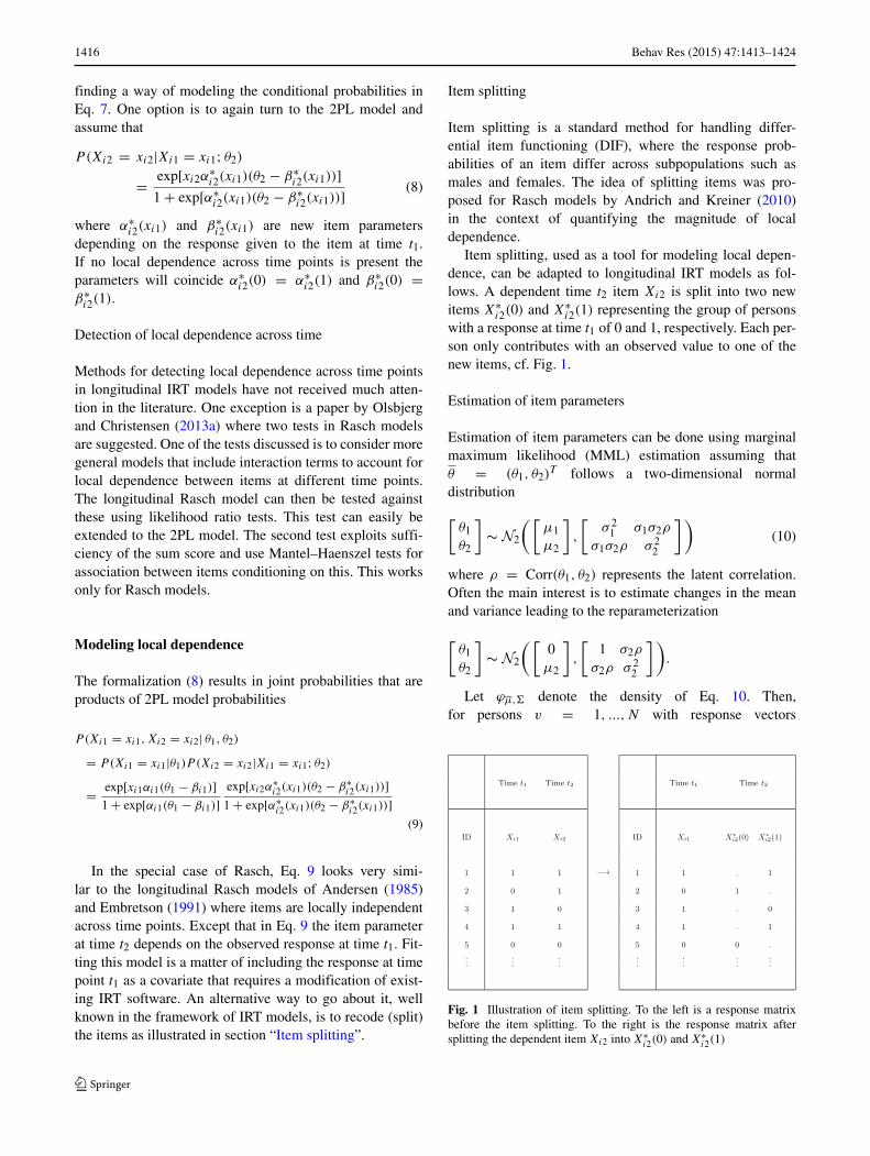
Item splitting, used as a tool for modeling local depen-dence, can be adapted to longitudinal IRT models as fol-lows. A dependent time t2 item Xi2 is split into two newitems X∗

i2(0) and X∗i2(1) representing the group of persons

with a response at time t1 of 0 and 1, respectively. Each per-son only contributes with an observed value to one of thenew items, cf. Fig. 1.

Estimation of item parameters

Estimation of item parameters can be done using marginalmaximum likelihood (MML) estimation assuming thatθ = (θ1, θ2)

T follows a two-dimensional normaldistribution

[θ1θ2

]∼ N2

( [μ1

μ2

],

[σ 21 σ1σ2ρ

σ1σ2ρ σ 22

])(10)

where ρ = Corr(θ1, θ2) represents the latent correlation.Often the main interest is to estimate changes in the meanand variance leading to the reparameterization

[θ1θ2

]∼ N2

( [0μ2

],

[1 σ2ρ

σ2ρ σ 22

]).

Let ϕμ,� denote the density of Eq. 10. Then,for persons v = 1, ..., N with response vectors

Fig. 1 Illustration of item splitting. To the left is a response matrixbefore the item splitting. To the right is the response matrix aftersplitting the dependent item Xi2 into X∗

i2(0) and X∗i2(1)

Behav Res (2015) 47:1413–1424 1417

Xv = (Xv11, ..., XvI1, Xv12, ..., XvI2), the marginal likeli-hood has the form

LM(α, β, μ, � | x1, ..., xN)

=N∏

v=1

∫

R2P(Xv = xv|θ)ϕμ,�(θ)dθ (11)

where α and β denote the vectors of item discriminationsand thresholds respectively, for both split and unsplit items.The probabilities in Eq. 11 are given by

P(Xv = xv|θ) =I∏

i=1

P(Xvi1 = xvi1|θ1)P (Xvi2

= xvi2|Xvi1 = xvi1; θ2)

I∏

i=1

(exp[xvi1αi1(θ1 − βi1)]1 + exp[αi1(θ1 − βi1)]

)

(exp[xvi2α

∗i2(xvi1)(θ2 − β∗

i2(xvi1))]1 + exp[α∗

i2(xvi1)(θ2 − β∗i2(xvi1))]

). (12)

We can not measure change in the latent variable with ameasurement instrument that changes completely. For thatreason, it is important that some of the items remains thesame, across time points, in the sense that

αi1 = α∗i2(0) = α∗

i2(1) and βi1 = β∗i2(0) = β∗

i2(1)

for i in some (reasonably sized) subset I0 ⊆ {1, ..., I }.Again, restrictions on the parameters are needed in order forthe model (11) to be identified. At each time point we haveto put restrictions on either the item or population parame-ters. One option is to require that either

∑Ii=1 βi1 = 0 and∏I

i=1 αi1 = 1, or that μ1 = 0 and σ 21 = 1, and similarly at

time t2.The model (11) can be estimated in SAS using the

NLMIXED procedure for fitting nonlinear mixed mod-els. MML estimation is carried out by maximizing anapproximation to the likelihood (11) integrating out the ran-dom effects. The SAS macro %LRASCH MML (Olsbjerg& Christensen, 2013b) is an implementation of the spe-cial case of Rasch models. In this implementation, adaptiveGaussian quadrature is used for integral approximation andthe Newton-Raphson algorithm for optimization. The SASmacro %LRASCH MML (Olsbjerg & Christensen, 2013b)works for incomplete data, and for this reason, local depen-dence across time points can be modeled according to Eq. 8.Whether the effect of local dependence is significant can beevaluated by comparing the likelihood in Eq. 11 to the like-lihood of the simple model based on the assumption of localindependence (6) in a likelihood ratio test.

Estimation of person location parameters

Usually, it is of interest to estimate change at the individ-ual level. In the previous section, we described how theitem parameters can be estimated by assuming a certaindistribution for the latent vector and then maximizing anapproximation to the marginal likelihood. Estimation of theperson parameters can be carried out in a similar mannerby substituting the item parameters in Eq. 12 by their MML

estimates α and β resulting in the likelihood function

LM(θ | x1, ..., xN) = L(α, β, θ | x1, ..., xN) (13)

where

L(α, β, θ | x1, ..., xN) =N∏

v=1

P(Xv = xv|θv)

is the joint likelihood with the estimated item parametersinserted. This corresponds to assuming a distribution ofthe item parameters which is degenerate in their estimatedvalues. Estimates of θv can be derived from Eq. 13 bynumerical optimization such as Newton–Raphson.

Thus, we can compute estimates θ = (θ1, θ2) and changescores θ2 − θ1 for each person. This can be done in themodel assuming local independence across time points andin a model that takes local dependence across time pointsinto account. It is then possible to evaluate whether localdependence across time points affects the conclusions aboutindividuals.

Simulation study

A simulation study was conducted to illustrate the implica-tions of local dependence across time points and to illustratethe advantage of splitting items. Responses were simulatedby (i) simulating person parameters from a two-dimensionalnormal distribution[

θ1θ2

]∼ N2

( [0μ

],

[1 0.50.5 1

] )

(ii) simulating responses at time 1 from a 2PL modelgiven the person and item parameters, and (iii) simulat-ing responses at time 2 from the same dichotomous Raschmodel with the exception that item thresholds for the locallydependent items were shifted by 1. More specifically, itemthresholds for these items were given as

β∗i2(0) = βi1 + 1 and β∗

i2(1) = βi1 − 1.

This means that at time 2 the item becomes more diffi-cult for those with a wrong response at time 1 and easier forthose with a correct response at time 1 in the case where 0

1418 Behav Res (2015) 47:1413–1424

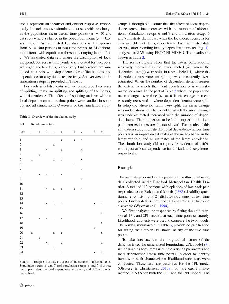
and 1 represent an incorrect and correct response, respec-tively. In each case we simulated data sets with no changein the population mean across time points (μ = 0) anddata sets where a change in the population mean (μ = 0.5)was present. We simulated 100 data sets with responsesfrom N = 500 persons at two time points, to 24 dichoto-mous items with equidistant thresholds ranging from −2 to2. We simulated data sets where the assumption of localindependence across time points was violated for two, four,six, eight, and ten items, respectively. Furthermore, we sim-ulated data sets with dependence for difficult items anddependence for easy items, respectively. An overview of thesimulation setups is provided in Table 1.

For each simulated data set, we considered two waysof splitting items, no splitting and splitting of the item(s)with dependence. The effects of splitting an item withoutlocal dependence across time points were studied in somebut not all simulations. Overview of the simulation study:

Table 1 Overview of the simulation study

LD Simulation setups

item 1 2 3 4 5 6 7 8 9

1 x x x

2 x

3 x x x

4 x

5 x x x x

6 x

7 x

8 x x x x

9 x

10

11 x x x x x

12

13

14 x x x x x

15

16 x

17 x x x x

18 x

19 x

20 x x x x

21 x

22 x x x

23 x

24 x x x

Setups 1 through 5 illustrate the effect of the number of affected items.Simulation setups 6 and 7 and simulation setups 6 and 7 illustratethe impact when the local dependence is for easy and difficult items,respectively

setups 1 through 5 illustrate that the effect of local depen-dence across time increases with the number of affecteditems. Simulation setups 6 and 7 and simulation setups 6and 7 illustrate the impact when the local dependence is foreasy and difficult items, respectively. Each simulated dataset was, after recoding locally dependent items (cf. Fig. 1),analyzed in SAS using PROC NLMIXED. The results areshown in Table 2.

The results clearly show that the latent correlation ρ

was only recovered in the rows labeled (ii), where thedependent item(s) were split. In rows labeled (i), where thedependent items were not split, ρ was consistently over-estimated. When the number of dependent items increasesthe extent to which the latent correlation ρ is overesti-mated increases. In the part of Table 2 where the populationmean changes over time (μ = 0.5) the change in meanwas only recovered in where dependent item(s) were split.In setup (i), where no items were split, the mean changewas underestimated. The extent to which the mean changewas underestimated increased with the number of depen-dent items. There appeared to be little impact on the itemparameter estimates (results not shown). The results of thissimulation study indicate that local dependence across timepoints has an impact on estimates of the mean change in thelatent variable, and on estimates of the latent correlation.The simulation study did not provide evidence of differ-ent impact of local dependence for difficult and easy items,respectively.

Example

The methods proposed in this paper will be illustrated usingdata collected in the Bradford Metropolitan Health Dis-trict. A total of 113 persons with episodes of low back painresponded to the Roland and Morris (1983) disability ques-tionnaire, consisting of 24 dichotomous items, at two timepoints. Further details about the data collection can be foundelsewhere (Waxman et al., 1998).

We first analyzed the responses by fitting the unidimen-sional 1PL and 2PL models at each time point separately.Likelihood ratio tests were used to compare the two models.The results, summarized in Table 3, provide no justificationfor fitting the simpler 1PL model at any of the two timepoints.

To take into account the longitudinal nature of thedata, we fitted the generalized longitudinal 2PL model (9),which handles both items with time-varying parameters andlocal dependence across time points. In order to identifyitems with such characteristics likelihood ratio tests wereconducted. These tests are described for the 1PL model(Olsbjerg & Christensen, 2013a), but are easily imple-mented in SAS for both the 1PL and the 2PL model. The

Behav Res (2015) 47:1413–1424 1419

Table 2 Simulation study results, 100 simulated data sets, N = 500 persons, 24 items (equidistant β1 = −2, . . . , β24 = 2)

True value μ=0 True value μ=0.5

Simulation μ ρ μ ρ

setup Mean SD Mean SD Mean SD Mean SD

1 (i) 0.01 0.06 0.50 0.04 0.51 0.06 0.51 0.04

(ii) 0.01 0.05 0.52 0.04 0.50 0.06 0.56 0.04

2 (i) 0.04 0.06 0.51 0.04 0.51 0.05 0.51 0.05

(ii) -0.02 0.05 0.55 0.05 0.50 0.05 0.57 0.04

3 (i) 0.00 0.06 0.51 0.05 0.50 0.05 0.50 0.05

(ii) 0.00 0.05 0.60 0.04 0.47 0.05 0.59 0.05

4 (i) 0.00 0.06 0.50 0.05 0.52 0.06 0.50 0.05

(ii) 0.00 0.05 0.62 0.04 0.49 0.06 0.62 0.04

5 (i) 0.00 0.06 0.50 0.05 0.50 0.06 0.50 0.05

(ii) 0.00 0.05 0.63 0.04 0.46 0.04 0.64 0.04

6 (i) 0.00 0.05 0.50 0.05 0.51 0.05 0.50 0.04

(ii) -0.02 0.05 0.54 0.05 0.48 0.06 0.54 0.05

7 (i) 0.00 0.04 0.50 0.05 0.53 0.06 0.50 0.05

(ii) 0.00 0.06 0.56 0.06 0.50 0.06 0.56 0.06

8 (i) 0.00 0.05 0.51 0.06 0.53 0.06 0.51 0.06

(ii) 0.00 0.05 0.60 0.06 0.51 0.06 0.60 0.06

9 (i) 0.01 0.06 0.51 0.05 0.54 0.06 0.51 0.05

(ii) -0.01 0.05 0.64 0.05 0.50 0.06 0.63 0.05

Average estimate of change in the latent mean μ and latent correlation ρ (true value 0.5). Assumption of local independence across time points isviolated for items 5, 20 (1), items 4, 8, 17, 21 (2), items 3, 8, 11, 14, 17, 22 (3), items 2, 5, 8, 11, 14, 17, 20, 23 (4), items 1, 3, 5, 8, 11, 13, 17, 20,22, 24 (5), items 1, 6, 11 (6), items 1, 3, 5, 7, 9, 11 (7), items 14, 19, 24 (8), items 14, 16, 18, 20, 22, 24 (9), (i): correct item splitting, (ii): no itemsplitting

assumption of time-invariant item parameters was firstinvestigated graphically using the estimates derived fromthe two unidimensional models. Centralized item thresholdsat the two time points are plotted against each other in Fig. 2and standardized item discriminations in Fig. 3.

Further investigation of the assumption of time-invariantitem parameters was done using a likelihood ratio test pro-posed by Olsbjerg and Christensen (2013a). This test is forDIF with respect to time based on MML estimation where,for each person, only responses at a single (randomly cho-sen) time point are used in order to get rid of possible localdependence. These tests suggested that item parameters for

Table 3 Likelihood ratio tests of the 1PL model against the 2PLmodel, separately at each time point

Time point Model −2 loglikelihood p-value

1 2PL 2348.3 < 0.0001

1PL 2429.3

2 2PL 2279.1 0.0003

1PL 2334.9Fig. 2 Item thresholds at time 1 and time 2

1420 Behav Res (2015) 47:1413–1424

Fig. 3 Item discriminations at time 1 and time 2

three items (items 2, 15, and 21) change over time. How-ever, in light of the large number of statistical tests and the

inherent risk of type I, we disregarded this evidence and wecontinued the analyses assuming that all item parameterswere the same at both time points. This corresponds wellwith what was observed in the plots in Figs. 2 and 3, wherethe estimates were relatively evenly scattered around thediagonal. As expected, the variation in the estimated itemdiscriminations across time points is noticeably larger thanfor the thresholds.

In order to identify items with local dependence acrosstime points, likelihood ratio tests were conducted. Thesetests were proposed by (Olsbjerg and Christensen 2013a) forRasch models but can easily be extended to the 2PL model.A total of eight out of the 24 items showed significant evi-dence of local dependence across time points. The resultsare summarized in Table 4.

We chose as our final model the 2PL model that incor-porates local dependence for the eight items with p-valuesbelow 5%. Estimates from this model can then be comparedto the estimates from the simpler 2PL model that ignoresthe dependence and where all items have equal parametersat the two time points. In Table 5, estimates of the popula-tion mean change and the latent correlation derived from thetwo models are displayed. The estimated population meanchange differs only slightly between the two models. The

Table 4 Item wording, estimated item parameters, and likelihood ratio tests for local independence across time points

no Item wording α (s.e.) β (s.e.) χ2 DF p-value

1 stay at home 2.66 (0.61) 1.56 (0.21) 4.1 4 0.3926

2 change position 0.59 (0.20) -2.13 (0.73) 15.8 4 0.0033

3 walk more slowly 1.96 (0.35) 0.57 (0.14) 6.6 4 0.1586

4 not doing jobs 2.39 (0.46) 0.96 (0.16) 8.7 4 0.0691

5 use handrail 1.58 (0.32) 1.40 (0.22) 5.5 4 0.2397

6 lie down 1.77 (0.33) 0.89 (0.17) 14.0 4 0.0073

7 hold on 1.43 (0.28) 1.20 (0.21) 3.6 4 0.4628

8 other people 2.49 (0.52) 1.36 (0.19) 10.5 4 0.0328

9 dressed more slowly 1.75 (0.33) 0.84 (0.16) 5.7 4 0.2227

10 stand up short periods 1.32 (0.25) 0.58 (0.17) 16.8 4 0.0021

11 try not to bend 1.59 (0.29) 0.55 (0.15) 2.0 4 0.7358

12 get out chair 1.54 (0.30) 1.20 (0.20) 4.2 4 0.3796

13 painful all the time 1.17 (0.23) 0.14 (0.16) 7.4 4 0.1162

14 turn over in bed 1.14 (0.23) 0.75 (0.19) 6.5 4 0.1648

15 appetite not good 0.98 (0.31) 3.33 (0.84) 18.9 4 0.0008

16 trouble putting on socks 1.25 (0.24) 0.56 (0.17) 18.6 4 0.0009

17 walk short distances 2.09 (0.40) 1.16 (0.18) 9.6 4 0.0477

18 sleep less well 0.94 (0.20) 0.08 (0.18) 8.4 4 0.0780

19 dress with help 1.55 (0.46) 2.88 (0.55) 3.0 4 0.5578

20 sit down most the day 2.77 (0.64) 1.58 (0.21) 0.8 4 0.9385

21 avoid heavy jobs 1.54 (0.28) 0.25 (0.15) 19.8 4 0.0006

22 more irritable 1.30 (0.25) 0.93 (0.20) 31.3 4 0.0000

23 upstairs more slowly 1.71 (0.33) 1.13 (0.19) 3.5 4 0.4779

24 stay in bed 1.93 (0.57) 2.61 (0.44) 5.2 4 0.2674

Behav Res (2015) 47:1413–1424 1421

Table 5 Population parameter estimates for Model 1, the simplemodel where no items are split for dependence and Model 2, the finalmodel where eight items are split for dependence

Parameter Model Estimate SE

Population mean change μ2 − μ1 1 0.231 0.09

2 0.229 0.11

Latent correlation ρ 1 0.71 0.06

2 0.65 0.07

estimated latent correlation decreases when items are splitfor dependence and this corresponds well with what wasobserved in the simulation study.

To get a sense of how it might affect the individualrespondents to ignore local dependence as compared tomodeling it, we investigate the estimated person locationsin the simple model and in the model taking local depen-dence across time into account. Keeping the item parametersfixed at their estimated values, we consider person locationestimates and estimates of the change

= θ2 − θ1

in the latent variable for Model 1 and Model 2. The results,presented in Table 6, reveal that generally the differencebetween the two models is not that big.

The two models do not differ with respect to the esti-mated time 1 person locations, but there appears to be morevariability in the incorrect Model 1. Regarding the personlocations at the second time point, there is a difference inthat Model 1 appears to underestimate the values. Again,there is more variability in the incorrect model. The differ-ence between the person time 2 person location estimatesfrom Model 1 and Model 2 were larger than the differencesbetween time 1 person location estimates.

Regarding change scores there was more variability whenusing the more correct model. A substantial variation in thedifference between values assigned to individuals wasobserved. A consequence of this variation is that the twomodels did not agree about who had a significant change

score. This occurred for five out of the 113 people respond-ing: 3 (2.7 %) who were considered to have a significant

value by Model 2, but not by Model 1 and 2 (1.8 %) whowere considered to have a significant value by Model 1only.

Discussion

The assumption of local independence in unidimensionalIRT models has been the focus of much research (Hoskens& De Boeck, 1997; Douglas et al., 1998; Ip, 2000, 2001,2002; Scott & Ip 2002). In unidimensional IRT models,violations of this assumption can be resolved by chang-ing the wording or the response categories of the items.Another solution is to use the sum of the dependent items asa so-called ’subtest’ (Andrich, 1985). Alternatively, a test-let model (Bradlow et al., 1999; Wang & Wilson, 2005) orother models taking account of local dependence (Hoskens& De Boeck, 1997; Ip, 2002) can be applied. In Rasch mod-els, a simple way of quantifying local dependence has beenproposed (Andrich and Kreiner, 2010).

In longitudinal studies where the same instrument is usedat several occasions to measure change in a latent variable,the assumption of local independence across time pointsmay well be violated. In that case, there is usually no desireto change the item content, and collapsing items across timepoints does not make sense in the context of measuringchange.

This paper described how local dependence across timepoints can be modeled in longitudinal IRT models. Basedon the method of item splitting by Andrich and Kreiner(Andrich and Kreiner (2010)), which has so far only beenused for quantification of local dependence in unidimen-sional models, we proposed a general method that can beused to test for and model local dependence across timepoints. It should be noted that in the Andrich and Kreinerapproach, the first item is discarded after recoding the sec-ond item, but that in the method proposed here we keep thetime 1 item along both versions of the time 2 item. Becausethe method is based on item splitting, a concept well known

Table 6 Summary of the estimated person locations (θ1 and θ2) and of the individual change scores = θ2 − θ1 for the 113 persons in the dataexample. Model 1 is the simple model where no items are split for dependence and Model 2 the true model where the eight items showing signsof local dependence are split

Model 1 Model 2 Difference

Mean SD Mean SD Mean (95 % ref. interval)

θ1 0.003 1.09 0.021 1.06 −0.02 (−0.32 to 0.15)

θ2 0.145 1.13 0.347 1.04 −0.02 (−0.51 to 0.47)

0.214 1.03 0.289 1.10 −0.01 (−0.554 to 0.488)

% significant 17 % 18 %

1422 Behav Res (2015) 47:1413–1424

for resolving differential item functioning (DIF), it can beused in existing software such as RUMM (Andrich et al.,2010)

The simulations incorporated local dependence in a waythat made it more likely for a person to give the sameresponse to an item at the two time points, than it wouldhave been in the case of local independence. By fittingthe simple model assuming local independence across timepoints for all items, we demonstrated some of the effectsof ignoring local dependence, one of them being that thedependence was mistakenly accounted for by the latentcorrelation ρ, which as a result was overestimated. Thesepatterns were visible in simulations with only a singledependent item and became even more pronounced whenmore items were dependent. Estimation of the change inthe mean of the latent variable was also affected by localdependence across time points. Results suggest that whenlocal dependence occurs for items located in the middleof the latent continuum (as was the case in the simula-tion study) the change in the mean of the latent variableis underestimated, whereas dependence for items located inone end of the continuum (as in the simulation study) leadto overestimation of the change in the mean of the latentvariable. This finding corresponds well with Marais (2009)who found that in certain circumstances local dependencewill exaggerate changes and in other circumstances it willmask them.

In the data example, an effect on the latent corre-lation, similar to those of the simulations, was foundwhen dependence was ignored, but regarding the esti-mated mean change of the latent variable, no differencewas found when splitting the items with signs of localdependence.

In the data examples and in the simulation study,estimation was done PROC NLMIXED estimating itemparameters and the two-dimensional latent distribution byMML estimation. For the special case of the Rasch (1PL)model, estimation can also be carried out in RUMM(Andrich et al., 2010) by splitting dependent items, fit-ting the model at each time point and then compar-ing person estimates. We considered dichotomous itemsadministered at two time points. The proposed methodis easily generalized to polytomous items because it isbased on the simple concept of item splitting. For thatreason, it can also be adapted to other IRT models.In principle, it is also straightforward to make exten-sions to accommodate more than two time points. How-ever, estimating the latent correlation matrix can becomecomputationally challenging. Moreover, the splitting pro-cedure can potentially become quite complex and leadto situations with sparse data if we allow for depen-dence structures that go beyond items at two consecutivetime points.

Differential item functioning identified in relation to timeis another phenomenon that occurs in longitudinal studies(Specht et al., 2011). This is often called item parame-ter drift (Wells et al., 2002; Miller & Fitzpatrick, 2009)and the assumption that item parameters are stable overtime should also be tested. Different methods for detectionof item parameter drift exist (Donoghue & Isham, 1998;DeMars, 2004; Galdin & Laurencelle, 2010). In the dataexample and in the simulation study, we assumed that itemparameters were stable over time, but for the special case ofRasch models, the SAS macro %LRASCH MML (Olsbjerg& Christensen, 2013b) can be used to test this assumptionusing likelihood ratio tests. Since local response dependenceformulated using item splitting is also implemented, thisyields a modeling framework where items that change overtime and items with local dependence across time points canbe included. This model can be fitted using two-dimensionalMML including three types of items: items with localdependence across time points, items with DIF across timepoints, and items with neither. Items with local dependenceacross time points are included by splitting the time 2 itemand estimating (α∗

i2(0), β∗i2(0)) and (α∗

i2(1), β∗i2(1)), items

with DIF across time points are included by the restrictionα∗

i2(0) = α∗i2(1) and β∗

i2(0)) = β∗i2(1)), and items with

neither can be included by the further restriction α∗i2(0) =

α∗i2(1) = αi1 and β∗

i2(0) = β∗i2(1) = βi1.

For investigating local dependence across time points fora single item, the proposed methodology yields a likelihoodratio test. In a realistic situation with many items in a test,care must be taken to control the type I error rate by adjust-ing for multiple testing using e.g., the Benjamini–Hochberg(1995) procedure.

The methodology outlined in this paper is a simpleway of accounting for local item dependence, while localperson dependence was not discussed. However, this canalso occur, and quite general methods for handling thisusing a four-level IRT model to simultaneously accountfor dual local dependence due to item clustering and per-son clustering have been proposed by (Jiao et al. 2012).The simple approach of taking dependence into accountusing item splitting proposed in this enables researchersto include local dependence in simpler multilevel mod-els (Kamata, 2001). However, when an item Xi2 is splitfor local dependence, fewer persons will contribute tothe estimation the new item parameters β∗

i2(0) and β∗i2(1)

than to the original parameter β2i . Hence, splitting itemsis at the cost of precision of the item parameter esti-mates and should only be done when there is evidenceof local dependence. In the data analysis, the samplesize was 113 and the 2PL model was fitted to the data,but the proposed methods were able to disclose evidenceof local dependence across time points, and to modelthese. However, the proposed methodology should not

Behav Res (2015) 47:1413–1424 1423

uncritically be used in applications with small samplesizes.

References

Adams, R.J., Wilson, M., Wang, W.-C. (1997). The multidimensionalrandom coefficients multinomial logit model. Applied Psycholog-ical Measurement, 21, 1–23.

Andersen, E.B. (1973). Conditional inference for multiple-choicequestionnaires. British Journal of Mathematical and StatisticalPsychology, 26, 31–44.

Andersen, E.B. (1985). Estimating latent correlations betweenrepeated testings. Psychometrika, 50, 3–16.

Andrich, D. (1985). A latent trait model for items with responsedependencies: Implications for test construction and analysis. InEmbretson, S. (Ed.) Test design: Contributions from psychology,education and psychometrics, chapter 9 (pp. 245–273). New York:Academic Press.

Andrich, D., Humphry, S., Marais, I. (2012). Quantifyinglocal, response dependence between two polytomous itemsusing the Rasch model. Applied Psychological Measurement, 36,309–324.

Andrich, D., & Kreiner, S. (2010). Quantifying response dependencebetween two dichotomous items using the Rasch model. AppliedPsychological Measurement, 34, 181–192.

Andrich, D., Sheridan, B., Luo, G. (2010). RUMM2030 [Computersoftware and manual]. Perth, Australia: RUMM Laboratory.

Benjamini, Y., & Hochberg, Y. (1995). Controlling the false discov-ery rate: A practical and powerful approach to multiple testing.Journal of the Royal Statistical Society. Series B, 57, 289–300.

Birnbaum, A.L. (1968). Latent trait models and their use in infer-ring an examinee’s ability. In Lord, F.M., & Novick, M.R. (Eds.)Statistical theories of mental test. Reading, MA: Addison-Wesley.

Bock, R.D., & Aitkin, M. (1981). Marginal maximum likelihood esti-mation of item parameters: An application of an em algorithm.Psychometrika, 46, 443–459.

Bousseboua, M., & Mesbah, M. (2010). Longitudinal latent Markovprocesses observable through an invariant Rasch model. In Rykov,V.V., Balakrishnan, N., Nikulin, M. (Eds.) Mathematical and sta-tistical models and methods in reliability (pp. 87–100). New York:.Springer.

Bradlow, E.T., Wainer, H., Wang, X. (1999). A Bayesian randomeffects model for testlets. Psychometrika, 64, 153–168.

DeMars, C.E. (2004). Detection of item parameter drift over multipletest administrations. Applied Measurement in Education, 17, 265–300.

Donoghue, J.R., & Isham, S.P. (1998). A comparison of procedures todetect item parameter drift. Applied Psychological Measurement,22, 33–51.

Douglas, J., Kim, H.R., Habing, B., Gao, E. (1998). Investigatinglocal dependence with conditional covariance functions. Journalof Educational and Behavioral Statistics, 23, 129–151.

Embretson, S. (1991). A multidimensional latent trait model formeasuring learning and change. Psychometrika, 56, 495–516.

Fischer, G.H., & Molenaar, I.W. (1995). Rasch models: Foundations,recent developments, and applications. New York: Springer.

Galdin, M., & Laurencelle, L. (2010). Assessing parameter invariancein item response theory’s logistic two item parameter model: AMonte Carlo investigation. Tutorials in Quantitative Methods forPsychology, 6, 39–51.

Holland, P.W., & Thayer, D.T. (1988). Differential item performanceand the Mantel-Haenszel procedure. In Wainer, H., & Braun,H.I. (Eds.) Test validity (pp. 129–145). Hillsdale, NJ: Erlbaum.

Holland, P.W., & Wainer, H. (1993). Differential item functioning.Hillsdale, NJ: Erlbaum.

Hoskens, M., & De Boeck, E. (1997). A parametric model for localdependence among test items. Psychological Methods, 2, 261–277.

Ip, E.H. (2000). Adjusting for information inflation due to local depen-dency in moderately large item clusters. Psychometrika, 65, 73–91.

Ip, E.H. (2001). Testing for local dependency in dichotomous andpolytomous item response models. Psychometrika, 66, 109–132.

Ip, E.H. (2002). Locally dependent latent trait model and the Dutchidentity revisited. Psychometrika, 67, 367–386.

Jiao, H., Kamata, A., Wang, S., Jin, Y. (2012). A multilevel test-let model for dual local dependence. Journal of EducationalMeasurement, 49(1), 82–100.

Jiao, H., Wang, S., Kamata, A. (2005). Modeling local item depen-dence with the hierarchical generalized linear model. Journal ofApplied Measurement, 6(3), 311–321.

Kamata, A. (2001). Item analysis by the hierarchical generalized linearmodel. Journal of Educational Measurement, 38, 79–93.

Kelderman, H. (1984). Loglinear Rasch model tests. Psychometrika,49, 223–245.

Kelderman, H. (1997). Loglinear multidimensional item responsemodels for polytomously scored items. In van der Linden, W., &Hambleton, R. (Eds.) Handbook of modern item response theory(pp. 287–304). New York: Springer.

Kreiner, S., & Christensen, K.B. (2004). Analysis of local dependenceand multidimensionality in graphical loglinear Rasch models.Communications in Statistics - Theory and Methods, 33, 1239–1276.

Kreiner, S., & Christensen, K.B. (2007). Validity and objectivity inhealth-related scales: Analysis by graphical loglinear Rasch mod-els. In von Davier, M., & Carstensen, C.H. (Eds.)Multivariate andmixture distribution Rasch models: Extensions and applications.New York: Springer.

Lazarsfeld, P.F., & Henry, N.W. (1968). Latent structure analysis.Houghton Mifflin, Boston, New York, Atlanta, Geneva (IL), Dal-las, Palo Alto.

Liu, L.C., & Hedeker, D. (2006). A mixed-effects regressionmodel for longitudinal multivariate ordinal data. Biometrics, 62,261–228.

Lord, F.M., & Novick, M.R. (1968). Statistical theories of mental testscores. Addison-Wesley.

Marais, I. (2009). Response dependence and the measurement ofchange. Journal of Applied Measurement, 10, 17–29.

Marais, I., & Andrich, D. (2008a). Effects of varying magnitude andpatterns of local dependence in the unidimensional Rasch model.Journal of Applied Measurement, 9, 105–124.

Marais, I., & Andrich, D. (2008b). Formalising dimension andresponse violations of local independence in the unidimensionalRasch model. Journal of Applied Measurement, 9, 200–215.

Miller, G.E., & Fitzpatrick, S.J. (2009). Expected equating error result-ing from incorrect handling of item parameter drift among thecommon items. Educational and Psychological Measurement, 69,357–368.

Muthen, B. (1979). A structural probit model with latent variables.Journal of the American Statistical Association, 74, 807–811.

Muthen, B. (1984). A general structural equation model with dichoto-mous, ordered categorical, and continuous latent variable indica-tors. Psychometrika, 49, 115–132.

Neyman, J., & Scott, E.L. (1948). Consistent estimates based onpartially consistent observations. Econometrika, 16, 1–32.

Olsbjerg, M., & Christensen, K.B. (2013a). Marginal and conditionalapproach to longitudinal Rasch models. Pub. Inst. Stat. Univ.Paris, 57, fasc, 1–2, 109–126.

1424 Behav Res (2015) 47:1413–1424

Olsbjerg, M., & Christensen, K.B. (2013b). SAS macro for marginalmaximum likelihood estimation in longitudinal polytomous Raschmodels. Research Report 11, Department of Statistics, Universityof Copenhagen.

Rasch, G. (1960). Probabilistic models for some intelligence andattainment tests. Copenhagen: Danish National Institute for Edu-cational Research.

Roland, M., & Morris, R. (1983). A study of the natural history ofback pain. 1. development of a reliable and sensitive measure ofdisability in low back pain. Spine, 8, 141–144.

Scott, S., & Ip, E.H. (2002). Empirical Bayes and item cluster-ing effects in a latent variable hierarchical model: A case fromthe national assessment of educational progress. Journal of theAmerican Statistical Association, 97, 409–419.

Specht, K., Leonhardt, J.S., Revald, P., Mandøe, H., Andresen, E.B.,Brodersen, J., Kreiner, S., Kjaersgaard-Andersen, P. (2011). Noevidence of a clinically important effect of adding local infusionanalgesia administrated through a catheter in pain treatment aftertotal hip arthroplasty. Acta Orthopaedica, 82(3), 315–320.

Thissen, D. (1982). Marginal maximum likelihood estimation for theone-parameter logistic model. Psychometrika, 47, 175–186.

Tjur, T. (1982). A connection between Rasch’s item analysis modeland a multiplicative Poisson model. Scandinavian Journal ofStatistics, 9, 23–30.

Wang, W.-C., & Wilson, M. (2005). The Rasch testlet model. AppliedPsychological Measurement, 29(2), 126–149.

Waxman, R., Tennant, A., Helliwell, P. (1998). Community surveyof factors associated with consultation for low back pain. BritishMedical Journal, 317, 1564–1567.

Wells, C.S., Subkoviak, M.J., Serlin, R.C. (2002). The effect of itemparameter drift on examinee ability estimates. Applied Psycholog-ical Measurement, 26, 77–87.

Yen, W.M. (1993). Scaling performance assessments: Strategies formanaging local item dependence. Journal of Educational Mea-surement, 30(3), 187–213.

Zwinderman, A.H., & van den Wollenberg, A.L. (1990). Robustnessof marginal maximum likelihood estimation in the Rasch model.Applied Psychological Measurement, 14, 73–81.