SANDIA REPORT SAND2009-0035 Unlimited Release Printed January 2009

Modeling Leaks from Liquid Hydrogen Storage Systems W. S. Winters Thermal/Fluid Science & Engineering Prepared by Sandia National Laboratories Albuquerque, New Mexico 87185 and Livermore, California 94550

Sandia is a multiprogram laboratory operated by Sandia Corporation, a Lockheed Martin Company, for the United States Department of Energy’s National Nuclear Security Administration under Contract DE-AC04-94AL85000.

Approved for public release; further dissemination unlimited.

2 2

Issued by Sandia National Laboratories, operated for the United States Department of Energy by Sandia Corporation. NOTICE: This report was prepared as an account of work sponsored by an agency of the United States Government. Neither the United States Government, nor any agency thereof, nor any of their employees, nor any of their contractors, subcontractors, or their employees, make any warranty, express or implied, or assume any legal liability or responsibility for the accuracy, completeness, or usefulness of any information, apparatus, product, or process disclosed, or represent that its use would not infringe privately owned rights. Reference herein to any specific commercial product, process, or service by trade name, trademark, manufacturer, or otherwise, does not necessarily constitute or imply its endorsement, recommendation, or favoring by the United States Government, any agency thereof, or any of their contractors or subcontractors. The views and opinions expressed herein do not necessarily state or reflect those of the United States Government, any agency thereof, or any of their contractors. Printed in the United States of America. This report has been reproduced directly from the best available copy. Available to DOE and DOE contractors from U.S. Department of Energy Office of Scientific and Technical Information P.O. Box 62 Oak Ridge, TN 37831 Telephone: (865) 576-8401 Facsimile: (865) 576-5728 E-Mail: reports@adonis.osti.gov Online ordering: http://www.osti.gov/bridge Available to the public from U.S. Department of Commerce National Technical Information Service 5285 Port Royal Rd. Springfield, VA 22161 Telephone: (800) 553-6847 Facsimile: (703) 605-6900 E-Mail: orders@ntis.fedworld.gov Online order: http://www.ntis.gov/help/ordermethods.asp?loc=7-4-0#online

3 3

SAND2009-0035 Unlimited Release

Printed January 2009

Modeling Leaks from Liquid Hydrogen Storage Systems

W. S. Winters Thermal/Fluid Science and Engineering

Sandia National Laboratories P.O. Box 5800

Livermore, California 94551-0969

Abstract

This report documents a series of models for describing intended and unintended discharges from liquid hydrogen storage systems. Typically these systems store hydrogen in the saturated state at approximately five to ten atmospheres. Some of models discussed here are equilibrium-based models that make use of the NIST thermodynamic models to specify the states of multiphase hydrogen and air-hydrogen mixtures. Two types of discharges are considered: slow leaks where hydrogen enters the ambient at atmospheric pressure and fast leaks where the hydrogen flow is usually choked and expands into the ambient through an underexpanded jet. In order to avoid the complexities of supersonic flow, a single Mach disk model is proposed for fast leaks that are choked. The velocity and state of hydrogen downstream of the Mach disk leads to a more tractable subsonic boundary condition. However, the hydrogen temperature exiting all leaks (fast or slow, from saturated liquid or saturated vapor) is approximately 20.4 K. At these temperatures, any entrained air would likely condense or even freeze leading to an air-hydrogen mixture that cannot be characterized by the REFPROP subroutines. For this reason a plug flow entrainment model is proposed to treat a short zone of initial entrainment and heating. The model predicts the quantity of entrained air required to bring the air-hydrogen mixture to a temperature of approximately 65 K at one atmosphere. At this temperature the mixture can be treated as a mixture of ideal gases and is much more amenable to modeling with Gaussian entrainment models and CFD codes. A Gaussian entrainment model is formulated to predict the trajectory and properties of a cold hydrogen jet leaking into ambient air. The model shows that similarity between two jets depends on the densimetric Froude number, density ratio and initial hydrogen concentration.

4 4

ACKNOWLEDGMENTS The author would like to acknowledge the support of Bill Houf, 08365 and Greg Evans, 08365 who provided their valuable time discussing and critiquing some of the ideas presented here. The turbulent buoyant entrainment model presented here for cold jets in ambient air is an extension of the model developed by Bill Houf for isothermal jets.

5 5

CONTENTS

MODELING LEAKS FROM LIQUID HYDROGEN STORAGE SYSTEMS ............................ 3

ACKNOWLEDGMENTS .............................................................................................................. 4

CONTENTS .................................................................................................................................... 5

FIGURES ........................................................................................................................................ 6

TABLES ......................................................................................................................................... 7

1. INTRODUCTION ...................................................................................................................... 9

2. SLOW LEAK MODELING ..................................................................................................... 11

2.1 Model for Zone 1: The Zone of Initial Entrainment and Heating .......................................................................... 14

2.2 Model for Zone 3: The Zone of Established Flow ................................................................................................. 22

2.3 Model for Zone 2: The Zone of Flow Establishment ............................................................................................ 26

2.4 Entrainment Model ................................................................................................................................................ 28

2.5 COLDPLUME Calculations .................................................................................................................................. 29

3. FAST LEAK MODELING ....................................................................................................... 33

3.1 Fast Leaks from Saturated Vapor Spaces ............................................................................................................. 35

3.2 Fast Leaks from Saturated Liquid Spaces ............................................................................................................. 37

3.3 Mach Disk Calculations for Fast Leaks ................................................................................................................ 39

4. NON-EQUILIBRIUM CONSIDERATIONS ......................................................................... 45

5. CONCLUSIONS...................................................................................................................... 47

6. REFERENCES ......................................................................................................................... 49

DISTRIBUTION........................................................................................................................... 53

6 6

FIGURES

Figure 1. Leaks from LH2 storage tank. ....................................................................................... 11

Figure 2. Flow zones for the turbulent entrainment model. ......................................................... 13

Figure 3. Temperature of exiting hydrogen as a function of storage pressure. ........................... 15

Figure 4. Quality of exiting hydrogen as a function of storage pressure. .................................... 15

Figure 5. Model for the zone of initial entrainment and heating. ................................................ 17

Figure 6. Air mole fraction as a function of temperature for flow exiting the zone of initial

entrainment and heating ................................................................................................................ 19

Figure 7. Normalized zone length as a function of assumed exit temperature. ........................... 21

Figure 8. Normalized exit diameter as a function of assumed exit temperature. ......................... 21

Figure 9. Coordinate system for buoyant jet. ............................................................................... 22

Figure 10. Comparison of two methods used to calculate BE. ..................................................... 28

Figure 11. Comparison of two jets with same initial velocity. .................................................... 30

Figure 12. Comparison of three jets with same initial Froude number. ...................................... 31

Figure 13. Comparison of two jets with same initial Froude number and density ratio. ............. 32

Figure 14. Fast leaks from LH2 storage tank. .............................................................................. 33

Figure 15. Exit quality and mass flux for a leak from the saturated vapor space. ....................... 36

Figure 16. Exit Mach number and temperature for a leak from the saturated vapor space. ........ 36

Figure 17. Exit pressure for a leak from the saturated vapor space. ............................................ 37

Figure 18. Exit quality and mass flux for a leak from the saturated liquid space. ....................... 37

Figure 19. Exit Mach number and temperature for a leak from the saturated liquid space. ........ 38

Figure 20. Structure of an under expanded jet, reproduced from [16]. ....................................... 40

Figure 21. Mach disk model ........................................................................................................ 41

Figure 22. Normalized Mach disk area and Mach number. ......................................................... 43

Figure 23. Mach disk mass flux and flow velocity. ..................................................................... 43

Figure 24. Mach disk temperature and quality. ........................................................................... 44

7 7

TABLES

Table 1. Saturation Table for Normal Hydrogen.. ............................................................ 14

8 8

THIS PAGE INTENTIONALY BLANK

9 9

1. INTRODUCTION

Saturated liquid hydrogen (e.g. 0.5-1.0 MPa) is currently being studied as possible transportation fuel in next-generation vehicles [1]. A need exists for developing codes and standards to support the wide-spread use liquid hydrogen. To develop these codes and standards the consequences of planned and unplanned hydrogen releases must be understood. This report documents several models for describing leaks or discharges from liquid hydrogen storage systems. The systems under consideration are mainly those used in supplying hydrogen for transportation. These systems include production storage tanks, tanker trucks and tanks located at vehicle fueling stations. Typically these systems store hydrogen in the saturated state at approximately five to ten atmospheres. Storage vessels are heavily insulated and sometimes actively cooled to minimize the rate of hydrogen boil-off. Leaks from liquid hydrogen storage systems can occur from spaces containing either saturated vapor or a saturated liquid. In most cases these leaks result in flashing two-phase flow as the hydrogen is exposed to atmospheric pressure. The models discussed here assume that flashing hydrogen behaves as a simple compressible substance in thermodynamic equilibrium. Thermodynamic models developed by NIST are used to calculate the state of leaking hydrogen and the state of hydrogen-air mixtures. NIST has incorporated its thermodynamic models into the program REFPROP [2] which can be used to generate tables and plots of thermodynamic and transport properties of important industrial fluids and their mixtures with an emphasis on hydrocarbons and refrigerants. While REFPROP is a stand-alone program, most of its subroutines are available in FORTRAN for linking into individual user applications. The models presented here have been cast into FORTRAN 95 programs that call the suite of REFPROP subroutines to model pure two-phase hydrogen and hydrogen mixtures with air. REFPROP is based on the most accurate pure fluid and mixture models currently available. Three models are implemented for the thermodynamic properties of pure fluids. These include equations of state explicit in Helmholtz energy, the modified Benedict-Webb-Rubin equation of state and an extended corresponding states model. Mixture property calculations utilize a model that applies mixing rules to the Helmholtz energy of the mixture components. A departure function is used to account for the deviation from ideal gas mixing. Thermal conductivity and viscosity are modeled three different ways: fluid-specific correlations, an extended corresponding states method or the friction theory method. The leaks or discharges considered here represent two extremes which are referred as “slow leaks” and “fast leaks”. A slow leak typically occurs through a microscopic crack at or near a fitting in the storage system. Frictional pressure drop along the leak path is large such that the hydrogen pressure at the exit is essentially atmospheric pressure. Leaks of this type can be modeled using entrainment models for turbulent buoyant jets or plumes provided suitable starting conditions can be derived for the exiting hydrogen. Section 2 of this report documents a plug-flow entrainment model that can be used to estimate flow area, velocity and air-hydrogen mass flow rates for a leak stream at one atmosphere and a “specified temperature”. Typically the temperature specified is high enough (e.g. 65 K) for air to exist in the mixture as a gas rather than a condensed phase. (REFROP cannot deal with both air and hydrogen as condensed phases.) The conditions provided by the plug-flow model are then used as starting conditions for a

10 10

turbulent buoyant jet/plume entrainment model that accounts for the effects of thermal as well as solutal buoyancy. Details of the jet/plume model are presented in Section 2. The fast leaks considered here are discharges that occur through relatively large openings. For these leaks the total pressure drop between the leak exit plane and the tank interior is negligible. A typical fast leak is the planned discharge of hydrogen that may occur through a valve during the transport of hydrogen from a tanker truck to the storage system at a filling station. These planned releases always occur from the saturated vapor portion of the storage tank. The models discussed in Section 3 show that the flow at the exit plane is usually choked regardless of whether the leak or venting occurs from a saturated liquid or saturated vapor space. Downstream of the exit plane the flow expands supersonically through a shock structure typical of underexpanded jets. When the flow finally becomes subsonic, it is still slightly compressible and has a relatively high speed (Mach numbers on the order of 0.4). Flows from fast leaks are generally modeled with CFD codes but they could be modeled using turbulent entrainment models if the leak stream approaches atmospheric pressure. A two-phase Mach disk model is documented in Section 3 for the purpose of providing subsonic boundary conditions for CFD models and turbulent entrainment jet/plume models.

11 11

2. SLOW LEAK MODELING Figure 1 illustrates the two kinds of slow leaks that can occur from a system storing hydrogen at a pressure sP . Since hydrogen is stored at its saturation state, the hydrogen storage temperature

sT is equal to the saturation temperature corresponding to the storage pressure, i.e.:

( )s sat sT T P (2.1)

For the system shown in Figure 1 leaks can occur from the saturated vapor space or saturated liquid space.

Figure 1. Leaks from LH2 storage tank.

For a slow leak we make the following assumptions:

Leak flows are quasi-steady. Hydrogen exits the leak at atmospheric pressure. In a slow leak through a microscopic

crack the frictional pressure drop along the leak path is large. Hence it is reasonable to assume the exiting hydrogen is at or near atmospheric pressure.

Potential and kinetic energy changes in the leaking flow stream are negligible. Slow leaks are by nature low velocity flows; hence it can be assumed that changes in kinetic energy are small when compared to enthalpy flux.

Heat exchange between the containment and the leaking flow stream is negligible. The assumption of adiabatic flow becomes reasonable for leaks that have established themselves for a period of time. In such leaks solid material surrounding the leak has had

12 12

sufficient time to equilibrate to a temperature that is nearly equal to the leak flow stream. Hence heat transfer from the containment to the exit stream is small when compared to the stream’s enthalpy. The adiabatic assumption is conservative from the standpoint of safety since it leads to colder more dense exiting hydrogen streams. Plumes or jets having these starting conditions require longer distances to dilute to non-flammable levels.

In all the leak scenarios discussed here it is assumed that the ambient is composed of still air at atmospheric pressure (.10133 MPa) and temperature of 295 K. Based on the above assumptions, the following steady flow energy equations can be written for saturated vapor and saturated liquid leaks:

2 2( )H I H g sm h m h P (2.2)

2 2( )H I H f sm h m h P (2.3)

where

2Hm is the mass flow rate of hydrogen through the leak, Ih is the initial value of the

hydrogen enthalpy as it enters the atmosphere, ( )g sh P is the enthalpy of saturated hydrogen

vapor at the storage pressure and ( )f sh P is the enthalpy of saturated hydrogen liquid at the

storage pressure. The transport of a slow leak through the atmosphere will be modeled using a series of three turbulent entrainment models. The models are shown schematically in Figure 2. The axial coordinate of the jet is designated by s. The three entrainment zones are: Zone 1: Zone of initial entrainment and heating ( 0 Os S )

Zone 2: Zone of flow establishment ( O ES s S )

Zone 3: Zone of established flow ( Es S )

The pressure in all three zones is assumed to be atmospheric. This is an important requirement for the application of turbulent entrainment models. In the first zone, “the zone of initial entrainment and heating”, pure hydrogen with a flow rate of

2Hm and an enthalpy of Ih enters on the left ( 0s ) at the leak exit plane. Air is entrained into

the leak jet such that the temperature of the hydrogen-air mixture exiting the zone on the right ( Os S ) is OT . OT is assumed to be the lowest temperature for which the properties of a

hydrogen-air mixture can be computed using available thermodynamic models. The details of the model for the zone of initial entrainment and heating are presented in Section 2.1. The second zone, “the zone of flow establishment”, provides the transition between the zone of initial entrainment and heating and the zone of established flow. A uniform flow of hydrogen and air at one atmosphere and temperature OT enters the zone on the left ( Os S ). In this zone the

uniform flow profiles make a transition to Gaussian profiles characteristic of fully established jet

13 13

flows before exiting on the right ( Es S ) . Details of the model for the zone of flow

establishment are presented in Section 2.3.

Figure 2. Flow zones for the turbulent entrainment model.

The third and by far the longest zone for the leak jet is “the zone of established flow.” In this zone the profiles for velocity and mixture properties vary with jet radius according to fully established Gaussian profiles that are constrained by the equation of state. The centerline values for velocity, hydrogen concentration and mixture enthalpy decrease with jet centerline distance. Furthermore the trajectory of the jet is influenced by buoyant forces due to local temperature and concentration differences. Details of the model for the zone of established flow are presented in Section 2.2. (Note: From the standpoint of introducing concepts and notation, it proves more convenient to discuss the model for the zone of established flow prior to discussing the zone of flow establishment.) The models for the zone of flow establishment and established flow are well known in the literature (see e.g. [3]) especially for liquid jets. They form the basis of a previous model developed by Houf and Schefer [4] to describe small-scale unintended releases of isothermal gaseous hydrogen. The present slow leak model for liquid hydrogen releases builds on this model by adding the energy equation so that buoyant forces resulting from the temperature

14 14

difference between the cold jet and the ambient can be accounted for in determining the trajectory of the jet. The zone of initial entrainment and heating is added to overcome difficulties in accounting for multiphase hydrogen and air mixing and to provide thermodynamically consistent starting conditions for the zone of flow establishment. The three zones making up the turbulent entrainment model are presented here in the context of slow leaks. However application of the three zones can also be made to fast leaks providing the leak stream has attained a pressure equal to the ambient pressure and changes in kinetic energy are small compared to the stream enthalpy.

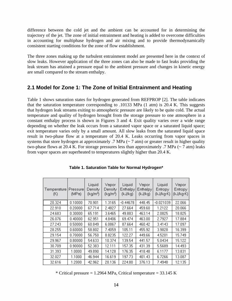
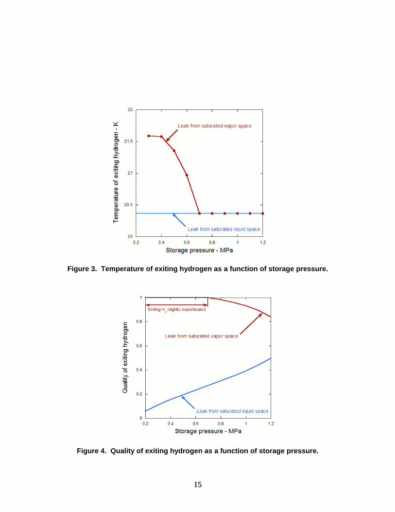
2.1 Model for Zone 1: The Zone of Initial Entrainment and Heating Table 1 shows saturation states for hydrogen generated from REFPROP [2]. The table indicates that the saturation temperature corresponding to .10133 MPa (1 atm) is 20.4 K. This suggests that hydrogen leak streams exiting to atmospheric pressure are likely to be quite cold. The actual temperature and quality of hydrogen brought from the storage pressure to one atmosphere in a constant enthalpy process is shown in Figures 3 and 4. Exit quality varies over a wide range depending on whether the leak occurs from a saturated vapor space or a saturated liquid space; exit temperature varies only by a small amount. All slow leaks from the saturated liquid space result in two-phase flow at a temperature of 20.4 K. Leaks occurring from vapor spaces in systems that store hydrogen at approximately .7 MPa (~ 7 atm) or greater result in higher quality two-phase flows at 20.4 K. For storage pressures less than approximately .7 MPa (~ 7 atm) leaks from vapor spaces are superheated to temperatures slightly higher than 20.4 K.

Table 1. Saturation Table for Normal Hydrogen*

* Critical pressure = 1.2964 MPa, Critical temperature = 33.145 K

15 15

Figure 3. Temperature of exiting hydrogen as a function of storage pressure.

Figure 4. Quality of exiting hydrogen as a function of storage pressure.

16 16

It is clear that the thermodynamics of leaking hydrogen can be complicated considering it is likely to be a two-phase mixture at extremely low temperature. The thermodynamics become more complicated as the exiting hydrogen stream entrains the surrounding ambient air. Near the exit any entrained air is likely to condense or even freeze resulting in a mixture that is difficult to characterize using equilibrium thermodynamics. Even a comprehensive thermodynamic model such as REFPROP [2] cannot characterize mixtures in which two or more of the mixture species exist in the liquid phase. To overcome this difficulty, a turbulent entrainment model will be used to model the first stage of the leaking hydrogen jet or plume. The following assumptions are used in developing a model for flow in zone 1, the zone of initial entrainment and heating:

The jet flow is turbulent and quasi-steady Since the flow is fully turbulent and steady, radial molecular diffusion is neglected

compared to radial turbulent transport. Radial turbulent transport is assumed to occur only at the jet periphery such that radial distributions of velocity concentration and enthalpy are uniform at any axial location in the jet, i.e. a plug-flow model is assumed.

Streamwise turbulent transport is negligible compared to streamwise convective transport Buoyancy is neglected due to the fact that the zone of initial entrainment and heating is

short and the trajectory of the jet is not significantly altered as a result of buoyant forces. Pressure is hydrostatic throughout the flow field and the thermodynamic pressure

throughout the flow field is one atmosphere. The jet remains axisymmetric, i.e. there are no circumferential variations in velocity,

enthalpy, density or concentration. The hydrogen and air are in thermodynamic equilibrium. Changes in kinetic and potential energy are negligible compared to changes in enthalpy. The contents of the storage tank are at a uniform temperature and pressure.

The entrainment model is schematically represented in Figure 5. The figure shows how continuity, momentum and energy are conserved in the zone of initial entrainment and heating. The exit temperature of the zone is an assumed value OT . The exit temperature is arbitrary but

modeling accuracy requires that this temperature be the lowest temperature where the exiting hydrogen-air mixture can exist as a gas (or the lowest temperature where REFPROP can compute the thermodynamic properties of the mixture). Keeping OT low will also cause the zone

of initial entrainment and heating to be short or even negligible compared to the remaining two zones that make up the leak jet.

17 17

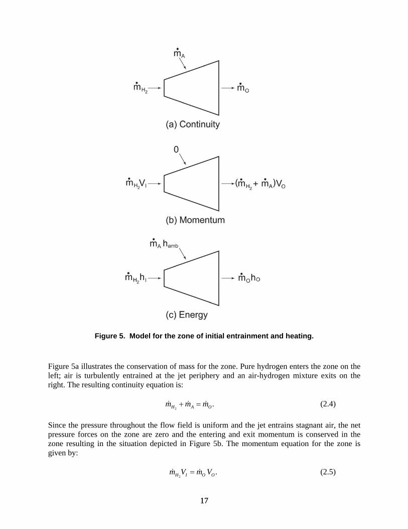
Figure 5. Model for the zone of initial entrainment and heating.

Figure 5a illustrates the conservation of mass for the zone. Pure hydrogen enters the zone on the left; air is turbulently entrained at the jet periphery and an air-hydrogen mixture exits on the right. The resulting continuity equation is:

2.H A Om m m (2.4)

Since the pressure throughout the flow field is uniform and the jet entrains stagnant air, the net pressure forces on the zone are zero and the entering and exit momentum is conserved in the zone resulting in the situation depicted in Figure 5b. The momentum equation for the zone is given by:

2.H I O Om V m V (2.5)

18 18

where IV is the velocity of hydrogen entering the zone (velocity at the leak plane) and OV is the

velocity of the air-hydrogen mixture exiting the zone. Figure 5c illustrates conservation of energy for the zone. Pure hydrogen enters the zone at the left with an known enthalpy, Ih ; air is entrained at the known ambient enthalpy, Ah and the air-

hydrogen mixture exits the right at the enthalpy, 0h resulting in the following energy equation:

2H I A amb O Om h m h m h (2.6)

where 0h is determined from the state specified by 0T , atmospheric pressure and the composition

of the exiting air-hydrogen mixture. Using Equation (2.4), the energy equation can be rewritten as:

2 2H I A amb H A Om h m h m m h (2.7)

The entrained air, Am necessary to bring the exiting air-hydrogen mixture to a temperature of OT

at atmospheric pressure may be determined iteratively from Equation (2.7). The procedure may be summarized as follows:

1. Set the exit mole fraction of air AOX to be zero.

2. Define a small increment for the exit mole fraction of air AOX

3. Set AO AO AOX X X

4. Compute 2 2

/ 1A H AO A AO Hm m X W X W where AW and 2HW are the molecular

weights of air and hydrogen respectively.

5. Compute the residual of the energy equation 2 2H I A A H A Om h m h m m h .

6. If the residual in step five is not zero or does not change sign repeat steps 3 through 5 until the assumed value for AOX satisfies the energy equation.

The above procedure was incorporated into a Fortran 95 computer program, ZONE1, to compute the entrained air necessary to cause the exiting air-hydrogen mixture to achieve a temperature of

0T at atmospheric pressure. The REFPROP subroutines were called by ZONE1 to compute

hydrogen, air and air-hydrogen mixture properties. Figure 6 shows how the exit mixture composition varies as a function of assumed exit temperature.

19 19

Figure 6. Air mole fraction as a function of temperature for flow exiting the zone of initial entrainment and heating

The results shown in Figure 6 are independent of

2Hm and the diameter of the leak. In order

compute the final diameter and length of the zone of initial entrainment and heating, it is necessary to consider the leak diameter and to make some assumptions regarding the entrainment of ambient air into the jet. Entrainment, E, for a fully turbulent jet is defined as

1

A

dmE

ds

(2.8)

where A is the ambient density (in this case the density of air at ambient conditions), m is the

total (hydrogen plus entrained air) jet mass flow rate and s is the axial coordinate of the jet. We shall approximate the gradient /dm ds as a constant for the zone of initial entrainment and heating such that

2 2

0

A H HO I A

O I O O

m m mm m mdm

ds S S S S

(2.9)

20 20

where the subscripts I and O are points in the flow at the entrance and exit of the zone of initial entrainment and heating. The origin of the jet (the leak plane), IS is assigned the value zero. The

length of the zone is oS can be expressed by combining Equations (2.8) and (2.9), i.e.

AO

A

mS

E

. (2.10)

The author is not aware of models or experiments which specifically address the entrainment of ambient air into fully turbulent jets containing multiphase hydrogen-air mixtures. However, considerable attention has been given to the entrainment of ambient air into fully turbulent gaseous jets and at least one source [29] states that entrainment rates for multiphase jets are identical to those of gaseous jets. Gebhart et. al. [3] summarizes a number of experimentally motivated models for entrainment from both quiescent and flowing ambients. Houf and Schefer [4] proposed an entrainment model based on an approach suggested by Hirst [5] in which the entrainment is characterized as the sum of momentum and buoyancy dominated contributions, e.g. mom buoyE E E (2.11)

momE , the contribution due to pure momentum is calculated from the Ricou and Spalding law [6]

which has the form

12 2 2

0.2824

I I Imom

amb

D VE

. (2.12)

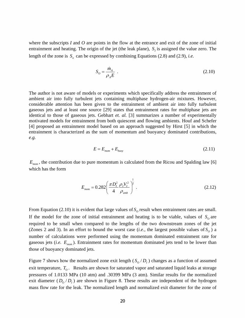
From Equation (2.10) it is evident that large values of OS result when entrainment rates are small.

If the model for the zone of initial entrainment and heating is to be viable, values of OS are

required to be small when compared to the lengths of the two downstream zones of the jet (Zones 2 and 3). In an effort to bound the worst case (i.e., the largest possible values of OS ) a

number of calculations were performed using the momentum dominated entrainment rate for gaseous jets (i.e. momE ). Entrainment rates for momentum dominated jets tend to be lower than

those of buoyancy dominated jets. Figure 7 shows how the normalized zone exit length ( /O IS D ) changes as a function of assumed

exit temperature, OT . Results are shown for saturated vapor and saturated liquid leaks at storage

pressures of 1.0133 MPa (10 atm) and .30399 MPa (3 atm). Similar results for the normalized exit diameter ( /O ID D ) are shown in Figure 8. These results are independent of the hydrogen

mass flow rate for the leak. The normalized length and normalized exit diameter for the zone of

21 21

initial entrainment and heating are only function of the assumed exit temperature, the storage pressure, the leak type (saturated liquid or saturated vapor) and the entrainment rate.

Figure 7. Normalized zone length as a function of assumed exit temperature.

Figure 8. Normalized exit diameter as a function of assumed exit temperature.

22 22

For the momentum dominated gaseous entrainment specified by Equation (2.12), Figures 7 and 8 indicate that the zone of initial entrainment and heating is relatively small (small oS and OD )

except for extremely buoyant jets as demonstrated in Section 2.4.

2.2 Model for Zone 3: The Zone of Established Flow The modeling techniques outlined here for the zone of established flow have been developed by Gebhart et. al. [3] and many others. The assumptions used are similar to those outlined in Section 2.1 except that the flow is no longer a “plug flow” and the influence of buoyancy is included in determining the trajectory of the jet or plume. The coordinate system used to describe jet trajectory and growth of the jet are shown in Figure 9. As mentioned previously, the jet axis lies along the streamwise s coordinate. The jet radial coordinate is r and the jet circumferential coordinate is . The angle between the jet axis and the x axis in the superimposed x-y-z Cartesian coordinate frame of Figure 9 is . The jet is assumed to be symmetrical about the x-y plane, hence the relationship between s, , x and y are given by:

cosdx

ds (2.13)

and

sindy

ds . (2.14)

Figure 9. Coordinate system for buoyant jet.

23 23

The integral equations for jet continuity, the two components of momentum, hydrogen concentration, and energy may be summarized as follows:

(continuity) 2

0 0

ambVrdrd Es

(2.15)

(x-momentum) 2

2

0 0

cos 0V rdrds

(2.16)

(y-momenturm) 2 2

2

0 0 0 0

sin ( )ambV rdrd grdrds

(2.17)

(concentration) 2

0 0

0VYrdrds

(2.18)

(energy) 2

0 0

0ambV h h rdrds

(2.19)

where , V, h, Y, g, and ambh are the jet density, velocity, enthalpy, hydrogen mass fraction,

gravitational constant and ambient enthalpy respectively. The ambient properties outside the jet are designated with the subscript “amb”. (“amb” is equivalent to the state “A” in the previous subsection.) A number of investigators including Albertson et. al. [7] and more recently Houf and Schefer [4] have shown that within the zone of established flow, the mean velocity profiles are nearly Gaussian and take the form 2 2exp( / )CLV V r B (2.20)

where CLV is the local centerline velocity, r is the radial coordinate and B is the characteristic jet

width or the radial distance at which V is equal to 1/e times CLV . Fan [8], Hoult et. al. [9] and

others have shown that scalar profiles within the jet are also Gaussian and can be expressed as:

2

2 2expamb CL amb

r

B

(2.21)

2

2 2expCL CL

rY Y

B

(2.22)

where CL , CLY are the local centerline density and hydrogen mass fraction respectively. The

parameter is discussed below.

24 24

The selection of a radial profile for h must be constrained in such a way as to satisfy the equation of state for the hydrogen air mixture. If reference enthalpies for each component are assigned a value zero at a temperature of zero, it follows that ph C T (2.23)

where pC is the mixture specific heat. Here we assume the hydrogen-air mixture behaves as a

calorically perfect ideal gas (specific heats of air and hydrogen have a negligible variation due to temperature). For a mixture of ideal gases it follows that

ambP MT

R (2.24)

where M is the mixture molecular weight and R is the universal gas constant. Substituting (2.24) into (2.23) yields

p ambC P Mh

R . (2.25)

The mixture specific heat and molecular weight can be expressed as

2(1 )

H Ap p pC YC Y C (2.26)

and

2

1

1

H A

Y YM

M M

(2.27)

where

2HpC and ApC are the specific heats of hydrogen and air and

2HM and AM are the

molecular weights. The radial distribution in h can be determined by combining Equations (2.21), (2.22), (2.25), (2.26) and (2.27). This complicated expression is represented here as ( , , , )CL CLh f Y B r (2.28)

The parameter in the radial distribution functions (Equations 2.21-2.22) represents the relative

spreading ratio between velocity and scalar properties , Y and h. This spreading ratio is related

to the turbulent entrainment Prandtl and Schmidt number effects.

25 25

Since the jet is assumed to be axisymmetric, there are no variations in and the Gaussian profiles given by Equations (2.20-2.22) may be substituted into the integral Equations (2.15-2.18) and integrated to yield the following ordinary differential equations:

(continuity) 2

2

2 1amb

CL amb amb CL

EdV B

ds

(2.29)

(x-mom.) 2

2 2

2

2cos 0

2 1CL amb amb CL

dV B

ds

(2.30)

(y-mom.)

22 2 2 2

2sin

2 2 1amb

CL amb CL amb CL

dV B B g

ds

(2.31)

(concentration) 2 0CL amb amb CL CL

dV B Y Y

ds (2.32)

The energy Equation (2.19) reduces to

(energy) 02 ( ) 0ambV h h rdr

s

. (2.33)

In Equation (2.33), V, and h, are replaced by their Guassian profiles from Equations (2.20), (2.21) and (2.28) respectively. The final form of this integral equation is not shown here. Equations (2.13-2.14), (2.29-2.33), represent a system of 7 ordinary differential equations and algebraic equations and 7 unknowns ( , ,x y , B, ,CL ,CLV and CLY ). COLDPLUME, a Fortran 95

computer program was written to solve this system of equations and predict the behavior of atmospheric pressure leaks from LH2 systems. The differential-algebraic solver DDASKR [10] was used in solving the equations. DDASKR is an improved version of the differential/algebraic system solver DASSL [11]. COLDPLUME solves the integral in Equation (2.33) numerically using the trapezoidal rule. Typically, the upper integration limit is replaced by 3B and 1000 equally spaced intervals ( dr ) are used to perform the integration. Numerical experiments were conducted in which the upper limit of integration was increased to 5B and 10,000 equally spaced intervals were used. The computed values for the seven dependent variables were unaffected in the first four significant figures. Several entrainment functions (see e.g. Equation 2.11) were investigated including the semi-empirical entrainment law developed by Houf and Schefer [4] for ambient temperature gaseous jets. An experimental program designed to measure entrainment for cold hydrogen jets is currently being planned. When this data becomes available it will be used to validate the COLDPLUME model.

26 26

Results from several COLDPLUME calculations are shown in Section 2.4.

2.3 Model for Zone 2: The Zone of Flow Establishment The model for the zone of flow establishment is used to provide the necessary starting conditions for the COLDPLUME program. This model is used to describe how the plug flow exiting the zone of initial entrainment and heating transforms into a fully developed jet flow with Gaussian profiles for velocity and the scalar transport quantities. The model for the zone of flow establishment is based on the model described by Gebhart et. al. [3] with a modification suggested by Houf [12]. The zone of flow establishment length, E OS S is taken from Abraham [13]:

2

2 2

2 2

2

( ) / 6.2, 40

( ) / 3.9 0.057 ,5 40

( ) / 2.075 0.425 ,1 5

( ) / 0,0 1

E O O

E O O

E O O

E O O

S S D Fr

S S D Fr Fr

S S D Fr Fr

S S D Fr

(2.34)

where Fr, the discharge densimetric Froude number is

( ) /

O

O amb O O

VFr

gD

. (2.35)

At Es S , the initial centerline velocity, the relative spreading ratios, the initial jet radius, and

the initial scalar centerline properties are given by: E CLV V (2.36)

1.16 (2.37)

/ 2 .707E O OB D D (2.38)

2

2

1.872

2CL amb CL ambE E

CL amb CL ambO O

h h Y Y

h h Y Y

. (2.39)

The present model for the zone of flow establishment utilizes Houf’s [12] expression for EB , the

jet radius at Es S . In the zone of flow establishment (see e.g. Figure 2) the expression that

describes the conservation of momentum from Os S to Es S is given by:

27 27

22

2

0 04O

O O

DV V rdrd

. (2.40)

Substituting the Gaussian profiles for velocity and density given by Equations (2.20) and (2.21) into Equation (2.40) yields the following expression:

2 2

2 22 4

2 1O amb amb CL

E O O

D

B

. (2.41)

The expression that describes the conservation of mass from Os S to Es S is given by:

22

0 0

( ) ( )4

OO amb O amb

DV V rdrd

. (2.42)

Substituting the Gaussian profiles for velocity and density given by Equations (2.20) and (2.21) into Equation (2.42) yields the following expression:

22

2 2

(1 )( )

4O

amb CL amb OE

D

B

. (2.42)

Equation (2.42) can be substituted into (2.41) to yield Houf’s expression for EB :

2

2 2

2(2 1)

1

OE

O

amb

DB

. (2.43)

Equation (2.43) can be compared to Equation (2.38) by substituting for the ratio /O amb and

noting that 1.16 . Figure 10 shows such a comparison. The value for amb was taken as the

density of air at 1 atm and 295 K. Values for O are densities of hydrogen-air mixtures at one

atmosphere and a range of temperatures assumed for OT (the exit temperature for the zone of

initial entrainment and heating). The previously discussed ZONE1 computer program and the REFPROP routines were used to calculate the densities. Results shown in Figure 10 are for leaks from both saturated liquid and saturated vapor spaces in a storage tank at a pressure of 7 atm. Values for the ratio 2( / )o ED B vary less than 6% over the range of temperatures considered here.

Houf’s use of the continuity Equation (2.42) neglects entrainment since it expresses the notion that the mass flow rate at Os S is identical to the mass flow rate at Es S .

28 28

Figure 10. Comparison of two methods used to calculate BE.

2.4 Entrainment Model In the absence of data for the entrainment of air into cold hydrogen jets, COLDPLUME utilizes the entrainment model of Houf and Schefer [4] which is based on an approach suggested by Hirst [5]. In this model the entrainment is characterized as the sum of momentum and buoyancy dominated contributions. This relationship was given in Equation 2.11 and is repeated here for convenience, ie. mom buoyE E E (2.44)

momE , the contribution due to pure momentum was given in Equation (2.12). The contribution

due to pure buoyancy is based on the following expression developed by Hirst [5]

2 2 sinbuoy CLL

E V BFr

(2.45)

where LFr , the local jet Froude number is given by

2

/CL

Lamb CL O

VFr

gD

. (2.46)

29 29

The empirical parameter 2 in Equation (2.45) was determined by Houf and Schefer [4] and

takes the form 4 2

2 17.313 0.11665 2.0771 10Fr Fr 268Fr (247a)

2 0.97 268Fr (247b)

where Fr is the jet densimetric Froude number given by Equation (2.35).

2.5 COLDPLUME Calculations COLDPLUME models jet or plume flow in Zones 2 and 3, the zone of flow establishment and the zone of established flow. Models for these zones have been presented in Sections 2.2 and 2.3. In this section COLDPLUME calculations will be presented to illustrate various aspects of jet behavior and similarity between jets. COLDPLUME predictions were compared to isothermal plume calculations made using the Houf and Schefer turbulent entrainment plume model [4]. When COLDPLUME is run with an initial hydrogen temperature equal to the ambient temperature, the predicted jet behavior is identical to that predicted by Houf and Schefer. COLDPLUME predictions for two leaks at two different initial hydrogen temperatures are shown in Figure 11. The starting temperatures for the two jets were 65 K and 265 K (ambient temperature) and each jet began as pure hydrogen ( 1.0OY ). The leak diameter, oD and

velocity, OV for each leak was 5 mm and 5 m/s respectively. The diameter and velocity were

chosen for illustration purposes only and are not necessarily proposed as “credible leaks.” The subscript “O” on the jet parameters , , ,o o o oD V Y Fr is meant to convey that these are jet starting

parameters corresponding to the jet trajectory location os S . All jets discussed in this section

began as an ideal gas with no initial entrainment and heating (i.e., Zone 1 is not present) hence os S o . Figure 11 shows the trajectory of each jet with the end point on each trajectory

curve representing the location where the centerline hydrogen concentration drops to 4% (0.04 mole fraction). As expected, the colder jet (65 K starting temperature) is less buoyant than the ambient temperature jet. This is evident from the slower rate of rise at the beginning of each jet. The relative buoyancy of the two jets is reflected in their initial densimetric Froude numbers. The densimetric Froude number for the ambient jet is 6.18, less than half that of the cold jet. Smaller Froude numbers imply more buoyant jets. Since the Froude numbers for both jets are relatively small, these jets are buoyancy dominated (see e.g. [4]). This is evident from the large vertical displacements on the y axis. Since the 65 K jet starts with a denser stream of hydrogen, the jet extends to a greater distance before entraining enough air to reduce the centerline concentration to 4%. Furthermore the 65 K jet has a higher Froude number. Equations (2.44-2.47) indicate that higher Froude number jets have lower entrainment rates.

30 30

Figure 11. Comparison of two jets with same initial velocity.

Figure 12 shows COLDPLUME predictions for three buoyant ( 10OFr ) jets; the first jet started

with pure hydrogen at ambient temperature; the second jet started with pure hydrogen at an initial temperature of 65 K and the third jet started with an air–hydrogen mixture having a hydrogen mass fraction of .3 and an initial temperature of 65 K. The trajectories of each jet are plotted with the x and y displacements normalized by the leak diameter OD . Since the Froude

number for the three jets is low, the trajectories are strongly influenced by buoyancy. This is evident in the large vertical displacements relative to the horizontal displacements. Houf and Schefer [4] have shown that the behavior of an ambient temperature (isothermal) turbulent jet is completely determined by the densimetric Froude number. This was verified using COLDPLUME. COLDPLUME was used to compute the trajectories of three different isothermal temperature jets having diameters of 1, 3 and 5 mm. The inlet velocities were adjusted to give a Froude number of 10. When these trajectories are plotted on x-y coordinates that are normalized by the leak diameter (e.g. Figure 12), the trajectories are identical. Furthermore the normalized positions where the jet reaches a centerline concentration of 4% are also identical. The COLDPLUME calculations shown in Figure 12 indicate that trajectory of non-isothermal jets starting as pure hydrogen is also fully characterized by the densimetric Froude. This is apparent from the trajectories of a 65K jet with leak diameters of 1, 3 and 5 mm. All three trajectories are identical when plotted on normalized coordinates. The results of Figure 12 show that Froude number similarity also holds when both the initial jet temperature and concentration are changed. The trajectories of a 65K air-hydrogen jet (initial

31 31

hydrogen mass fraction of .3, arbitrarily selected) with leak diameters of 1, 3 and 5 mm are also are identical when plotted on normalized coordinates.

Figure 12. Comparison of three jets with same initial Froude number.

The COLDPLUME results seem to indicate that the Froude number jet similarity rule holds for all jets having the same initial density ratio /O amb . That is all jets having the same Froude

number and density ratio will have identical trajectories when plotted on normalize coordinates regardless their starting jet diameter or velocity. This is indeed the case. However, an additional constraint must be imposed when predicting the location in the trajectory where the hydrogen concentration achieves a particular value. This point is illustrated in Figure 13 which shows the normalized trajectory of two jets each of which has the same Froude number and initial density ratio. As in Figures 11 and 12, the trajectory of each jet is plotted up to the point where the centerline concentration drops to 4% (.04 mole fraction). The two jets shown in Figure 13 each have a Froude number of 10 and an initial density ratio of .3158 and each jet has the same trajectory. However the jet having the lower initial hydrogen concentration ( 0.3OY ) reaches

the 4% limit more rapidly. Hence complete similarity between two jets can only be assured if the initial Froude number, density ratio and hydrogen concentrations are the same.

32 32

Figure 13. Comparison of two jets with same initial Froude number and density ratio.

33 33

3. FAST LEAK MODELING Figure 14 illustrates the two kinds of fast leaks that can occur from a system storing hydrogen at a pressure sP . ( sP is typically 0.5-1.0 MPa.) As was the case for the slow leak modeling of

Section 2, it is assumed that hydrogen is stored at its saturation state and the hydrogen storage temperature sT is equal to the saturation temperature corresponding to the storage pressure, i.e.:

( )s sat sT T P (3.1)

For the system shown in Figure 14 leaks can occur from the saturated vapor space or saturated liquid space.

Figure 14. Fast leaks from LH2 storage tank. For a fast leak we make the following assumptions:

Leak flows are quasi-steady There is negligible total pressure loss from the tank stagnation conditions to the exit

conditions, i.e., fast leaks are associated with large holes and relatively short frictionless flow paths through the containment wall.

Potential energy changes in the leaking flow stream are negligible. Heat exchange between the containment and the leaking flow stream is negligible. The

flow is fast enough that any heat loss is small compared to the enthalpy of the flow stream.

The hydrogen behaves as a simple compressible substance in thermodynamic equilibrium.

34 34

Hydrogen two phase flows are homogeneous with the liquid and vapor phases having the same velocity.

The contents of the storage tank are at a uniform temperature and pressure. In large storage tanks some temperature stratification may occur causing the temperature to be non-uniform but here we assume that such stratification has negligible influence on modeling results.

As was the case for slow leaks, all fast leak scenarios discussed here assume that the ambient is composed of still air at atmospheric pressure (.10133 MPa) and temperature of 295 K. Subject to the assumptions listed above, the following quasi-steady statement of the conservation of energy can be written:

21

2S I Ih h V (3.2)

where h is the enthalpy per unit mass of hydrogen, V is velocity and the subscripts S and I refer to the states of hydrogen in the vessel and at the leak plane respectively. The state designated by S is the stagnation state for hydrogen in the vessel, i.e., the state of all hydrogen in the vessel a short distance from the leak where the velocity is zero. Since no total pressure losses are assumed for flow between states S and I and the flow is assumed to be adiabatic, it follows that S Is s (3.3)

where s is the entropy per unit mass of hydrogen. The value of Sh varies depending on whether the fast leak is occurring from the saturated vapor

space or the saturated liquid space. In either case Sh only depends on the value of the storage

pressure, sP and can be expressed as follows:

(saturated liquid leak) S f sh h P (3.4)

(saturated vapor leak) S g sh h P (3.5)

Where fh and gh are the enthalpy per unit mass of saturated liquid and saturated vapor

respectively. Equations (3.2) – (3.5) are sufficient to determine the state of hydrogen exiting the vessel (i.e., state I) and its velocity. These values are independent of the leak area.

35 35

A Fortran 95 program, FLASHEXIT1, was written to determine the state and velocity of hydrogen exiting a fast leak. The program makes use of equations (3.2)-(3.5) and the previously discussed REFPROP subroutines. The algorithm used by FLASHEXIT1 is summarized as follows:

1. I Ss s

2. I SP P

3. P ( 0) for accurate convergence

4. I IP P P

5. , ( , )I h s P I Ih f s P

6. , ( , )I a s P I Ia f s P

7. 2I S IV h h

8. If I IV a , STOP, solution is found, flow is choked.

9. If I ambP P , STOP, solution found, flow is unchoked.

10. Go to step 4 The functions ,h s Pf and ,a s Pf represent the REFPROP subroutines for enthalpy and sound

speed respectively. For decreasingly small values of , the inequalities used in steps 8 and 9 approach equalities and the algorithm results in a solution having greater precision.

3.1 Fast Leaks from Saturated Vapor Spaces The model for fast leaks or discharges from saturated vapor spaces describes flow caused by an unintended release of hydrogen through a large hole in a storage tank. The model can also be used to describe an intended release of hydrogen through a valve. The latter discharge is the kind planned release that occurs during the off-loading of hydrogen from a tank truck to a filling station. FLASHEXIT1 was used to model fast leaks from the saturated vapor space. Figures 15 and 16 illustrate how the thermodynamic state and velocity of hydrogen at the leak plane (state I) varies with storage pressure. These results are independent of the leak size. For the range of storage pressures considered here, the hydrogen at exit plane is two-phased with the quality decreasing as the storage pressure increases. The mass flux through the leak is nearly proportional to the storage pressure except for the lowest pressures where the leak is unchoked ( 1Ma ). Hydrogen temperatures for the leak vary from approximately 20 K at low storage pressures to nearly 26 K at the highest storage pressure (10 atm).

36 36

Figure 15. Exit quality and mass flux for a leak from the saturated vapor space.

Figure 16. Exit Mach number and temperature for a leak from the saturated vapor space.

For storage pressures greater than .3 MPa (~3 atm) the flow through the leak is choked. As a result the leak exit pressure is considerably higher than atmospheric pressure (see e.g. Figure 17). Because of this, the previously discussed techniques used to model slow leaks (i.e. atmospheric pressure turbulent entrainment models) cannot be used for fast leaks unless they are applied further downstream where the leak jet has achieved ambient pressure. Modeling is further complicated by the fact that the exiting flow is both compressible and two-phase.

37 37

Figure 17. Exit pressure for a leak from the saturated vapor space.

3.2 Fast Leaks from Saturated Liquid Spaces FLASHEXIT1 was also used to model fast leaks from saturated liquid spaces. Results are shown in Figures 18 and 19. These results are independent of leak size. Many of the trends previously observed for saturated vapor leaks apply to saturated liquid leaks. Leak flows are choked, two-phase and have high pressures when compared to the ambient. Saturated liquid leaks have greater liquid content with qualities less that 20%. Mass fluxes are nearly double those of saturated vapor leaks for the same storage pressure.

Figure 18. Exit quality and mass flux for a leak from the saturated liquid space.

38 38

Figure 19. Exit Mach number and temperature for a leak from the saturated liquid space.

While making the saturated liquid calculations presented in this section, it was discovered that many of the sound speed values returned from the REFPROP subroutines were inconsistent or in error. Often a value of zero was returned indicating the sound speed was undefined for that particular state. In order to overcome this difficulty the sound speed for the saturated liquid leak calculations were computed from the thermodynamic definition of sound speed, i.e.

s

Pa

. (3.6)

The derivative, s

P

at a particular state point was calculated numerically using two

consecutive calls to a two-phase subroutine. The entropy, s at the state point was used as one of the independent variables. The second independent variable was pressure, density, or enthalpy. Hence the sound speed was calculated three different ways. The calculations for the three sound speeds 1 2 3, ,a a a are summarized as follows:

1a : PSFLSH called twice with ( 1,P s ) and ( 2 ,P s ). Values for 1 2, returned.

2a : DSFLSH called twice with ( 1, s ) and ( 2 , s ). Values for 1 2,P P returned.

3a : HSFLSH called twice with ( 1,h s ) and ( 2 ,h s ). Values for 1 2 1 2, , ,P P returned.

where 1 2 1 2 1 2, , , , ,P P h h represent small perturbations in density, pressure and enthalpy at the

state point of interest and PSFLSH, DSFLSH and HSFLSH are the REFPROP flashing subroutines. The density and pressure values returned from the REFPROP subroutines where used to calculate the sound speed using the following expression:

39 39

2 1

2 1

P Pa

. (3.7)

For sufficiently small perturbations about the state point, the three computed sound speeds were essentially equal. In addition to calculating the sound speed for saturated mixtures, the above method was used to compute the sound speed in hydrogen gas over a range of states for which the ideal gas equation of state is known to be valid. In all cases the sound speed computed from Equation (3.7) was

found to be equal to the theoretical value for an ideal gas, i.e. RT where is the ratio of

specific heats, R is the gas constant and T is the absolute temperature. The homogeneous equilibrium model (HEM) described here for modeling fast leaks from saturated liquid spaces may under predict choked flow rates. Limitations of the HEM model are discussed in Section 4.

3.3 Mach Disk Calculations for Fast Leaks It is apparent from the previous two subsections that fast leaks are choked unless the storage pressure is very low (~3 atm or less). Downstream of the choke the flow will expand supersonically and pass through a shock structure before finally reaching the ambient pressure. Modeling the flow in this highly compressible region can be difficult even for multidimensional CFD codes. In this case the problem is further complicated by the fact that the flow exiting the leak is two-phase. A number of pseudo source models have been proposed to eliminate the need to model supersonic expansion and shocking in leak flows. The models attempt to replace the choked flow at the leak with a “source” of flow at atmospheric pressure. Typically the total temperature (energy content) and mass flow rate are preserved and the source flow occurs through a larger area than the actual leak area. The assumption inherent in the application of a pseudo source model is that jet behavior at some distance from the source is essentially the same as it would have been had the source been the actual choked flow. Birch et.al. [14-15] proposed source models based on continuity, momentum and energy balances for a control volume surrounding the supersonic flow and shock structure. Flows are assumed to be uniform in cross-section (i.e. plug flow). Assumptions are made regarding the pressure forces on the control volume and the exit temperature. More recently Winters and Evans [16] proposed a source model that includes the features of supersonic expansion and shocking back to atmospheric pressure. The model is referred to as the “Mach disk model.” Their model was applied to gaseous flows. In this section the Mach disk model is used to compute “equivalent” two-phase atmospheric conditions for a choked fast leak. Figure 20 illustrates the structure of an underexpanded jet. The figure which is reproduced from Christ et. al. [17], shows the flow expanding supersonically from the choke point where the Mach number is 1 to a Mach disk or planar shock where it

40 40

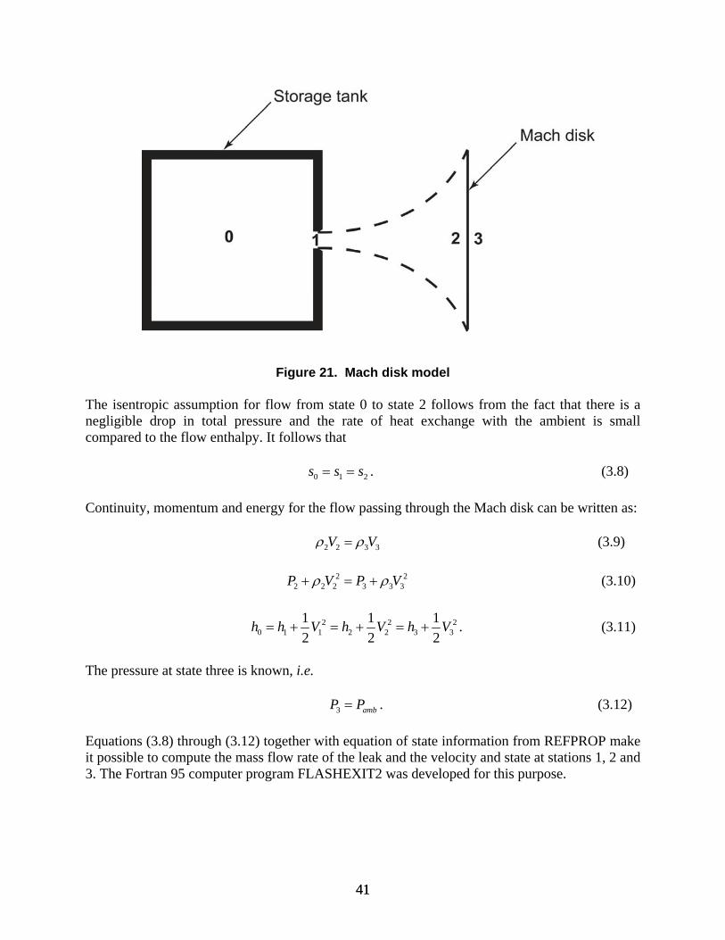
transitions to a subsonic flow ( 1.0M ). Most of the supersonic flow is enclosed by expansion fans, intercepting shocks and waves. An idealized version of the under expanded jet is shown in Figure 21. The figure shows the choked flow exiting a storage tank. Flow at tank stagnation conditions (state 0) accelerates to the choke point (state 1). From there it expands supersonically to a position just upstream of the Mach disk (state 2) before “shocking up” to atmospheric pressure (state 3). The following assumptions are made for the fast leak Mach disk model:

The flow is quasi-steady. Flow expands isentropically from state 0 to 1. Flow is choked at state 1. Flow expands isentropically from state 1 to state 2. All flow passes through the single Mach disk between states 2 and 3. No ambient air is entrained into the supersonic region. The pressure at state 3 is ambient pressure. The hydrogen in the flow behaves as a simple compressible substance in thermodynamic

equibrium. Potential energy and buoyancy in the flow are neglected

Figure 20. Structure of an under expanded jet, reproduced from [16].

41 41

Figure 21. Mach disk model

The isentropic assumption for flow from state 0 to state 2 follows from the fact that there is a negligible drop in total pressure and the rate of heat exchange with the ambient is small compared to the flow enthalpy. It follows that 0 1 2s s s . (3.8)

Continuity, momentum and energy for the flow passing through the Mach disk can be written as: 2 2 3 3V V (3.9)

2 2

2 2 2 3 3 3P V P V (3.10)

2 2 20 1 1 2 2 3 3

1 1 1

2 2 2h h V h V h V . (3.11)

The pressure at state three is known, i.e. 3 ambP P . (3.12)

Equations (3.8) through (3.12) together with equation of state information from REFPROP make it possible to compute the mass flow rate of the leak and the velocity and state at stations 1, 2 and 3. The Fortran 95 computer program FLASHEXIT2 was developed for this purpose.

42 42

FLASHEXIT2 makes use of the following algorithm:

1. 3 ambP P

2. P where is a small number 3. Set 2 ambP P (a guess)

4. 2 2P P P (a new guess)

5. 2 0s s

6. 2 , 2 2( , )h P sh f P s

7. 2 , 2 2( , )P sf P s

8. 2 0 22V h h

9. 2 33 2

2 2

P PV V

V

10. 22

323 2 2 2

VVh h

11. 2 23

3

V

V

12. 3 , 3 3( , )EOS P hf P h

13. 3 3 0EOS go to step 4

14. Solution converged where ,h P sf , ,P sf and ,P hf are REFPROP equation of state relationships. The precision of

the calculation can be improved by allowing to approach zero. For a sufficiently small value of the inequality in step 13 approaches an equality and convergence results in an accurate calculation of the state downstream of the Mach disk. FLASHEXIT2 was used to compute the conditions downstream of a Mach disk as a function of the storage pressure. The leak was assumed to be from the saturated vapor space. The results are shown in Figures 22-24. These results are independent of leak area.

43 43

Figure 22. Normalized Mach disk area and Mach number.

Figure 23. Mach disk mass flux and flow velocity.

Figure 22 shows the normalized Mach disk area. The normalizing factor is the leak area. The Mach disk area increases linearly with the storage pressure. At the maximum pressure considered (~ 8 atm) the Mach disk area is nearly 11 times the leak area. The Mach number downstream of the Mach disk decreases with increasing storage pressure. The Mach number values (.43-.33) indicate the flow exiting the Mach disk is slightly compressible. Figure 23 shows mass flux at the Mach disk and the velocity downstream of the Mach disk. The density of hydrogen exiting the Mach disk is not shown here but it may be determined by dividing the mass flux by the velocity.

44 44

Figure 24 shows the temperature and quality of the hydrogen downstream of the Mach disk. The temperature is relatively constant at approximately 20.4 K (the saturation temperature of hydrogen at 1 atm) and the quality is nearly one over most of the storage pressure range. At the highest storage pressure considered the quality drops to .965.

Figure 24. Mach disk temperature and quality.

The condition of the hydrogen exiting the Mach disk of a fast leak is extremely cold (20.4K) and may be slightly wet (two-phase). As was the case for slow leaks discussed in Section 2.1, air entrained into such a stream results in a mixture that is difficult to characterize thermodynamically. It seems clear that the plug flow model of the type used for the zone of initial entrainment and heating in slow leak modeling will also be required for fast leaks. Once the hydrogen-air mixture is elevated in temperature to approximately 65 K it can be treated as a mixture of ideal gases and traditional entrainment models or CFD analysis can then proceed. An application of the slow leak entrainment model is valid providing the kinetic energy in the leak stream is small compared to the enthalpy.

45 45

4. NON-EQUILIBRIUM CONSIDERATIONS

While modeling releases of non-equilibrium liquid-vapor hydrogen mixtures is beyond the scope of this work, it seems appropriate that some attention be given to those situations for which the models documented here may not apply. The models discussed in previous sections are intended to describe the behavior of hydrogen leaking from the high pressure (2-10 atm) storage systems. Since we are addressing liquid hydrogen storage systems, these leaks can occur from saturated liquid or saturated vapor spaces. Inherent in all the discussions thus far is the assumption that the leaking hydrogen behaves as a simple compressible substance in global thermodynamic equilibrium. Furthermore it is assumed that the velocities of the vapor and liquid phases are identical. As the pressure in a leaking hydrogen stream is decreased from the storage value to one atmosphere, the global equilibrium assumption requires that the local liquid and vapor phase temperatures be equal to the saturation temperature corresponding to the local stream pressure. This is most certainly true for slow leaks since there is sufficient time to equilibrate liquid and vapor phase temperatures as the pressure is lowered. The equilibrium assumption is also likely to be true for fast leaks from the saturated vapor space. For such leaks the quality of the mixture tends to be high with a very small amount of liquid, which if finely dispersed will rapidly achieve the saturation temperature. It has been shown (see e.g. reference [18]) that homogeneous equilibrium models tend to under predict critical (choked) flows for leaks from saturated liquid spaces and other two phase regions where the quality is low. The phase equilibrium assumption may be violated for rapid depressurization of saturated liquid since there is insufficient time to transfer enough energy between the phases to maintain global equilibrium. The homogeneous assumption may lead to additional inaccuracies due unequal liquid and vapor phase velocities. Several non-equilibrium and non-homogeneous models have been proposed to predict critical two phase flow. A homogeneous “frozen” or non-equilibrium critical flow model has been proposed by a number of researchers including Henry and Fauske [19]. Moody [20] and Fauske [21] have proposed critical flow models that account for unequal phase velocities. Fauske [22] has proposed a semi-empirical critical flow model for critical flows exiting tubes having a range of length-to-diameter ratios. The equilibrium assumption has the potential of breaking down for fast leaks occurring from saturated liquid spaces particularly if the leaks are massive or if the liquid in the stream is not sufficiently dispersed. The transition from stored liquid hydrogen to gaseous hydrogen at one atmosphere is a blowdown process or the rapid boiling of a liquid by lowering its pressure. The present author has shown (see e.g. [23-25]) that if the blowdown occurs at rapid enough rate, departure from global thermodynamic equilibrium can occur. During blowdown of a liquid, the vaporization process begins at a finite number of nucleation sites. These nucleation sites typically occur at microscopic cavities on the surfaces of the containment structure or on impurities suspended in the liquid. Spontaneous nucleation in the bulk liquid is also possible but difficult to achieve. After a brief period of inertially dominated bubble growth, the temperature of the growing vapor phase becomes equal to the saturation temperature corresponding to the local pressure. The liquid adjacent to the liquid-vapor interface is also at the saturation temperature. However, the remainder of the liquid will be superheated with respect to the local mixture pressure. The

46 46

lowering of the liquid temperature to its saturation value can only occur at a liquid-vapor interface. Hence heat conduction, convection and the total area of the liquid-vapor interface has an influence on the rate at which the liquid reaches the saturation temperature. While local thermodynamic equilibrium may be occurring at every point in the liquid and vapor, during a rapid blowdown, the liquid and vapor may not be in global equilibrium because some portion of the liquid phase is superheated with respect to the vapor. Edwards and O’Brien [26] and the present author [23-25] have studied the blowdown of water and Freon 12 from long tubes. Pressure and temperature measurements were used to document a significant departure from global equilibrium during the blowdown process.

Several studies have shown that during a massive spill of liquid hydrogen some “rainout” of the liquid may occur. In some cases liquid hydrogen may pool briefly on the ground while the vaporization process occurs. These are clear examples of situations in which the liquid-vapor hydrogen mixture is not in global thermodynamic equilibrium. During vaporization portions of the raining liquid or liquid pool are superheated with respect to the vapor that is being formed. Heat transfer from the surroundings and vaporization at the liquid-vapor interface eventually cause the liquid to disappear forming a movable cloud of hydrogen vapor. Witcofski [27] documented experiments conducted to study the dispersion of hydrogen clouds resulting from a spill of 5.7 cubic meters of liquid hydrogen. He concluded that pooling was so brief that measures to dike and contain the liquid hydrogen are unnecessary. Spill and vaporization induced turbulent mixing with ambient air served to rapidly evaporate the liquid hydrogen. Venetsanos and Bartzis [28] reference additional experimental efforts to study hydrogen cloud formation from liquid hydrogen spills. These studies all document situations in which the liquid-vapor mixture is not in global thermodynamic equilibrium.

47 47

5. CONCLUSIONS

This report documents a series of equilibrium-based models for studying leaks from liquid hydrogen storage systems. The models make use of the REFPROP subroutines developed by NIST to specify the states of multiphase hydrogen and air-hydrogen mixtures. Except for some problems encountered in predicting properties for low quality hydrogen vapor-liquid mixtures (problems with sound speed) and low temperature air-hydrogen mixtures (problems for mixture temperatures below 65 K), the REFPROP subroutines performed well predicting properties over the entire range of states pertinent to liquid hydrogen storage.

Leaks modeled here were classified as slow leaks and fast leaks. Slow leaks are characterized by large pressure drops through small cracks. In a slow leak hydrogen enters the ambient at or near one atmosphere. Fast leaks are characterized by negligible total pressure drop (between the tank stagnation point and the leak plane) through relatively large holes. Fast leaks nearly always result in choked flow at the exit plane of the leak regardless of whether the leak originates from the saturated liquid or saturated vapor portion of the storage system.

The hydrogen entering the ambient from a slow leak in the containment adjacent to a saturated vapor space is slightly superheated for storage pressures less than .7 MPa (~ 7 atm). For storage pressures greater than .7MPa the leak becomes two-phase with the quality decreasing as storage pressure is increased. For a storage pressure of 1.0 MPa (~10 atm) the quality of the vapor-hydrogen mixture is approximately 0.9. Slow leaks from saturated liquid spaces result in two-phase hydrogen mixtures with qualities increasing from 0.03 to 0.5 over a storage pressure range of 0.2 to 1.2 MPa.

In order to avoid the complexities of supersonic flow, a single Mach disk model is proposed for fast leaks that are choked. The velocity and state of hydrogen downstream of the Mach disk leads to a more useful subsonic boundary condition. However, the hydrogen temperature exiting all leaks (fast or slow, saturated liquid or saturated vapor) is very nearly equal to 20.4 K, the saturation temperature corresponding to 1 atm. At these temperatures, any entrained air would likely condense or even freeze leading to an air-hydrogen mixture that cannot be characterized by the REFPROP subroutines. For this reason a plug flow entrainment model is proposed to cover a short zone of initial entrainment and heating. The model predicts the quantity of entrained air required to bring the air-hydrogen mixture to a temperature of approximately 65 K. At this temperature the mixture can be treated as a mixture of ideal gases and is much more amenable to modeling with Gaussian entrainment models and CFD codes. For slow leaks the zone of initial entrainment and heating is shown to be a relatively short distance, typically under 35 leak diameters.

This report documents a Gaussian entrainment model that can be used to predict the trajectory and concentration profiles in a cold hydrogen jet injected into ambient air. The model can be applied to fast or slow leaks providing the appropriate Mach disk model is used (for fast leaks only) and the starting temperature for the calculation is approximately 65 K. The Gaussian entrainment model shows that similarity between two jets depends on the densimetric Froude number, density ratio and initial hydrogen concentration.

48 48

THIS PAGE INTENTIONALY BLANK

49 49

6. REFERENCES [1] W. Peschka, “State of Hydrogen Cryofuel Technology for Internal Combustion

Engines,” Hypothesis Conference, Grimstad, Norway, August 1997. [2] E. W. Lemmon, M. L. Huber, M. O. McLinden, “NIST Reference Fluid

Thermodynamic and Transport Properties-REFPROP,” Version 8 User’s Guide, U. S. Department of Commerce Technology Administration, National Institute of Standards and Technology, Standard Reference Data Program, Gaithersburg, Maryland 20899, April, 2007.

[3] B. Gebhart, D. S. Hilder and M. Kelleher, “The Diffusion of Turbulent Buoyant

Jets,” Advances in Heat Transfer, Vol. 16, Academic Press, Inc., Orlando, Florida, 1984.

[4] W. Houf, R. Schefer, “Analytical and Experimental Investigation of Small-Scale

Unintended Releases of Hydrogen,” International Journal of Hydrogen Energy, Vol. 33, pp 1435-1444, 2008.

[5] E. A. Hirst, “Analysis of Buoyant Jets within the Zone of Flow Establishment,” Oak

Ridge National Laboratory Report, ORNL-TM-3470, 1971. [6] F. P. Ricou and D. B.Spalding, “Measurement of Entrainment by Axisymmetrical

Turbulent Jets,” Journal of Fluid Mechanics, Vol. 11, pp 21-31,1961. [7] M. L. Albertson, Y. B. Dai, R. A. Jensen and H. Rouse, “Diffusion of Submerged

Jets,” Transactions of the American Society of Civil Engineers, Vol. 115, pp 639-697, 1950.

[8] L. H. Fan, “Turbulent Buoyant Jets into Stratified and Flowing Ambient Fluids,”

Rep. No. KH-R-15, W. M. Keck Laboratory, California Institute of Technology, Pasadena, 1967.

[9] D. P. Hoult, J. A. Fay, and L. J. Forney, “A Theory of Plume Rise Compared with

Field Observations,” Journal of Air Pollution Control Association, Vol. 19, 585-590, 1969.

[10] L. R. Petzold, P. N. Brown, A. C. Hindmarsh, and C. W. Ulrich, “DDASKR –

Differential Algebraic Solver Software,” Center for Computational Science & Engineering, L-316, Lawrence Livermore National Laboratory, P.O. Box 808, a private communication with L. R. Petzold.

[11] L. R. Petzold, “A Description of DASSL: A Differential/Algebraic Solver System

Solver,” SAND82-8637, Sandia National Laboratories, Livermore, CA, September, 1982.

[12] W. Houf, private communication, September, 2008.

50 50

[13] G. Abraham, “Horizontal Jets in Stagnant Fluid of Other Density,” J. Hydraul.

Div.Am.Soc.Civ.Eng. Vol. 9, 1965 [14] A. D. Birch, D. R. Brown, M. G. Dodson, and F. Swaffield, “The Structure and

Concentration decay of High Pressure Jets of Natural Gas,” Combustion Science and Technology, Vol. 36, 1984.

[15] A. D. Birch, D. J. Hughes, and F. Swaffield, “Velocity Decay of High Pressure Jets,”

Combustion Science and Technology, Vol. 36, 1987. [16] W. S. Winters and G. H. Evans, “Final Report for the ASC Gas-Powder Two-Phase

Flow Modeling Project AD2006-09,” SAND2006-7579, Sandia National Laboratories, Livermore, CA, January 2007.

[17] S. Crist, P. M. Sherman and R. R. Glass, “Study of Highly Underexpanded Sonic

Jet,” AIAA Journal, Vol. 4, No. 1, January, 1966. [18] M. L. Corradini, Fundamentals of Multiphase Flow, copyright M. L. Corradini,

University of Wisconsin, Madison WI 53706, available on the internet at http://wins.engr.wisc.edu/teaching/mpfBook/main.html.

[19] R. E. Henry and H. K. Fauske, “ The Two-Phase Critical Flow of One-Component

Mixtures in Nozzles, Orifices and Short Tubes,” Journal of Heat transfer, p. 179, May, 1971.

[20] F. J. Moody, “Maximum Flow Rate of a Single Component Two-Phase Mixture,”

Journal of Heat Transfer, Transactions ASME Series C, Vol. 87, No. 1, p.134, February, 1965.

[21] H. K. Fauske, “Contribution to the Theory of Two-Phased One-Component Critical

Flow,” Argonne National Laboratory Report, ANL-6633, 1961. [22] H. K. Fauske, “The Discharge of Saturated Water Through Tubes,” Chemical

Engineering Progress Symposium Series, Vol. 61, p. 210, 1965. [23] W. S. Winters Jr., “Non-Equilibrium Blowdown in Long Pipes,” PhD Thesis, The

University of Michigan, Ann Arbor, 1978. [24] W. S. Winters and H. Merte, Jr., “Non-Equilibrium Effects in Pipe Blowdown with

R-12,” Proceedings of the Two-Phase Flow and Heat Transfer Symposium, CONF-761039, Pergaman Press, Fort Lauderdale, Florida, October 1976.

[25] W. S. Winters and H. Merte, Jr., “Analysis of Pipe Blowdown,” Nuclear Science and

Engineering, Vol. 69, No. 3, March, 1979.

51 51

[26] A. R. Edwards and T. P. O’Brien, “Studies of Phenomena Connected with the Depressurization of Water Reactors,” Journal of British Nuclear Society, Vol. 9, 1970.

[27] R. D. Witcofski, “Dispersion of Flammable Vapor Clouds Resulting from Large

Spills of Liquid Hydrogen,” Langley Research Center, Hampton, VA. [28] A. G. Venetsanos and J. G. Bartzis, “CFD Modeling of Large-Scale LH2 Spills in

Open Environment,” International Journal of Hydrogen Energy, Vol. 32, 2007. [29] “Methods for the Calculation of Physical Effects,” Yellow Book, CPR 14E (Part 1),

p. 2.44, Editors: C. J. H. van den Bosch and R. A. P. M. Weterings, The Committee for the Prevention of Disasters by Hazardous Materials, The Hague, 1997.

52 52

THIS PAGE INTENTIONALY BLANK

53 53

DISTRIBUTION 1 University of California Attn: Professor Ralph Greif Department of Mechanical Engineering Berkeley, CA 94720 1 Charles Powars St. Croix Research 5525 Fern Drive San Jose, CA 95124 1 MS0748 J. L. LaChance 06761 1 MS9054 R. W. Carling 08300 1 MS9054 S. K. Griffiths 08300 1 MS9161 A. E. Pontau 08360 1 MS9409 C. D. Moen 08365 1 MS9409 D. E. Dedrick 08365 1 MS9409 G. H. Evans 08365 1 MS9409 W. G. Houf 08365 5 MS9409 W. S. Winters 08365 1 MS9052 J. O. Keller 08367 1 MS9051 R. W. Schefer 08367 2 MS9018 Central Technical Files 08944 2 MS0899 Technical Library 04536

54 54

R. Burgess Chair LH2 Task 9 Robert_burgess@nrel.gov Electronic copy D. Farese Member LH2 Task 9 faresedj@airproducts.com Electronic copy

A. Unione Member LH2 Task 9 al.unione@parsons.com Electronic copy

W. Houf Member LH2 Task 9 will@sandia.gov Electronic copy S. Woods Member LH2 Task 9 stephen.s.woods@nasa.gov Electronic copy F. Gavelli Member LH2 Task 9 fgavelli@exponent.com Electronic Copy P. May National Fire Protection Association pmay@NFPA.org Electronic copy