Embed Size (px)
Citation preview

MODELING INFILTRATION IN A STORMWATER CONTROL MEASURE USING
MODIFIED GREEN AND AMPT
A Thesis
Presented to
The Faculty of the Department of Civil and Environmental Engineering
Villanova University
In Partial Fulfillment
Of the Requirements for the Degree of
Master of Water Resources Engineering
by
Ryan S. Lee
May 2011
Copyright 2011 by Ryan S. Lee

MODELING INFILTRATION IN A STORMWATER CONTROL MEASURE USING
MODIFIED GREEN AND AMPT
by
Ryan S. Lee
May 2011
____________________________ ____________ Robert G. Traver, Ph.D., PE, D.WRE Date Professor, Department of Civil and Environmental Engineering Faculty Advisor
____________________________ ____________ Andrea L. Welker, Ph.D., PE Date Professor, Department of Civil and Environmental Engineering Faculty Advisor
____________________________ ____________ Ronald A. Chadderton, Ph.D., P.E. Date Chairman, Department of Civil and Environmental Engineering
____________________________ ____________ Gary A. Gabriele, Ph.D. Date Dean, College of Engineering

Acknowledgements
I would like to thank Dr. Traver for his several years of support, and for teaching me
much about water resources engineering. I would like to thank also Dr. Welker for her help.
Special thanks to my wife Ann, who has supported me through my education and career change,
and thanks to my son Max for occasionally taking a nap so that I could have time to do some
work!
iv
ABSTRACT
MODELING INFILTRATION IN A STORMWATER CONTROL MEASURE USING
MODIFIED GREEN AND AMPT
by Ryan S. Lee
Villanova University, 2011
SUPERVISOR: Dr. Robert G. Traver, P.E., D. WRE.
Accurate predictive models of infiltration in stormwater control measures (SCMs) are not
readily available. While it is common to model infiltration at the watershed level using
stochastic models such as the SCS Curve Number Method, stochastic models require a lot of data
to develop, and unfortunately that data is not available or has not been processed for SCMs.
Physics-based models (solutions to the Richards equation) are desirable, however they are too
complex to parameterize and can tend to increase computational times. The Green and Ampt
solution of the Richards equation is a physics-based solution that is appropriate for infiltration
where standing water is not present, and it is easy to parameterize and simple to solve because of
the approximations made to develop the solution. This has been recognized and Green and Ampt
has been made available for use in EPA’s Stormwater Management Model (SWMM) for storage
basin nodes, which can be used to model SCMs.
However, the Green and Ampt model used for watersheds has two major shortcomings when
used to model an SCM: the SCM has a 2- or 3-dimensional shape that affects the infiltration rate,
and engineered soil layers add an important dimension to the performance. In SCM models, the

v
importance of infiltration variability is increased because inflow rates can be an order of
magnitude higher than rainfall alone, and pond emptying time is an important variable. To
rectify these shortcomings, additions were made to the Green and Ampt model to account for the
shape of the basin and the depth of water therein, soil layering, and the variability of infiltration
due to temperature (other variabilities from storm size and soil wetness are inherent in the Green
and Ampt solution).
This modified Green and Ampt model was correlated against data from two distinct
bioinfiltration rain gardens on Villanova University’s campus, showing that the model is able to
predict the infiltration proces over a wide range of conditions. Data from the sites were analyzed
to show that about half of the natural variability of infiltration rates comes from a combination of
storm size and temperature variation, and the rest of the variability is from soil moisture
conditions. The correlations also produced a lower-bound distribution of soil moisture
conditions, showing that typical values for Green and Ampt infiltration parameters are
conservative engineering estimates (95th percentile conservative) for the sites analyzed.
Therefore, this study concludes that the Green and Ampt method, once modified to account for
temperature dependence, soil layers, and water depth and shape dependence, is complete and
accurate for use in predicting infiltration rates in SCMs, especially for conservative soil moisture
conditions. It is recommended that these modifications be incorporated into the USEPA SWMM
program for widespread use.

vi
TABLE OF CONTENTS ABSTRACT ................................................................................................................................................. iv
TABLE OF CONTENTS ............................................................................................................................. vi
LIST OF TABLES ...................................................................................................................................... vii
LIST OF FIGURES ................................................................................................................................... viii
1. INTRODUCTION ................................................................................................................................ 1
2. PROBLEM STATEMENT ................................................................................................................... 3
3. LITERATURE REVIEW ..................................................................................................................... 4
4. METHODS ......................................................................................................................................... 14
4.1. Infiltration Model ........................................................................................................................ 14
4.2. Basin Shape Dependence ............................................................................................................ 15
4.3. Temperature Dependence ........................................................................................................... 21
4.4. Layered Soils .............................................................................................................................. 21
4.5. Green and Ampt Soil Parameters ................................................................................................ 23
4.6. Computational Methods .............................................................................................................. 27
4.7. Summary of Model Assumptions/Approximations .................................................................... 28
5. MODEL SENSITIVITIES .................................................................................................................. 29
5.1. Hydraulic Conductivity Sensitivity ............................................................................................. 29
5.2. Matric Suction Sensitivity ........................................................................................................... 30
5.3. Soil/Water Characteristic Curve Sensitivity ............................................................................... 33
5.4. Basin Shape Sensitivity ............................................................................................................... 35
6. MODEL APPLICATIONS ................................................................................................................. 39
6.1. Villanova Traffic Island .............................................................................................................. 39
6.1.1. Site Overview ...................................................................................................................... 39
6.1.2. Model Correlation ............................................................................................................... 40
6.2. Fedigan Rain Garden .................................................................................................................. 49
6.2.1. Site Overview ...................................................................................................................... 49
6.2.2. Model Correlation ............................................................................................................... 50
6.3. Discussion ................................................................................................................................... 54
7. CONCLUSION ................................................................................................................................... 57
8. RECOMMENDATIONS .................................................................................................................... 58
9. REFERENCES ................................................................................................................................... 59

vii
LIST OF TABLES Table 5.1 Results of bowl shape sensitivity analysis. ................................................................................. 36 Table 5.2 Results of model runs comparing with and without shape factor. .............................................. 37 Table 6.1 Correlation results for three events at FRG. ............................................................................... 51

viii
LIST OF FIGURES Figure 4.1 Discretization of infiltration bowl geometry. ............................................................................ 16 Figure 4.2 Plot of average event recession rates from the Villanova Traffic Island from 2003-2007. ....... 26 Figure 5.1 Plot of change in conductivity (K) vs. change in average recession rate (RR). ........................ 30 Figure 5.2 Plot of changes in matric suction (ψ) vs. change in average recession rate (RR), centered at values of ψ near field capacity (82 inches is center). .................................................................................. 32 Figure 5.3 Plot of changes in matric suction (ψ) vs. change in average recession rate (RR), centered at low values of ψ near saturation (20 inches is center). ........................................................................................ 32 Figure 5.4 Average recession rate (RR) vs. matric suction (ψ) for Loamy Sane with SWCC varied. ....... 34 Figure 5.5 Average recession rate (RR) vs. matric suction (ψ) for Sandy Clay Loam with SWCC varied. .................................................................................................................................................................... 35 Figure 6.1 Villanova traffic island while ponded........................................................................................ 40 Figure 6.2 Model and actual depth vs. time for a 4.54 inch rain event. Constant infiltration rate is visible. .................................................................................................................................................................... 42 Figure 6.3 Model and Actual depth vs. time for a 0.35 inch rain event. Decreasing infiltration rate is visible. ......................................................................................................................................................... 43 Figure 6.4 Comparison of average recession rates between best-fit model and data. ................................. 44 Figure 6.5 Distribution of matric suction values from model correlations. ................................................ 45 Figure 6.6 Distribution of event mean infiltration rates from model correlations. ..................................... 46 Figure 6.7 Plot of linear regression of mean infiltration rate as a function of K and ψ only. The black line is the cross-section of the plane of best-fit. ................................................................................................. 47 Figure 6.8 Distribution of matric suction values after reducing the conductivity by 20% and 40%. ......... 48 Figure 6.9 Fedigan bioinfiltration rain garden. Inflow V-notch weir shown. ............................................. 50 Figure 6.10 Depth vs. time plot from a 0.95 inch rainfall event. Only a brief surge in ponding. .............. 51 Figure 6.11 Depth vs. time plot from a 1.95 inch rainfall event. ................................................................ 52 Figure 6.12 Depth vs. time plot from a 7.42 inch rainfall event. ................................................................ 53 Figure 6.13 Inflow and infiltration rates during the 7.42 inch rainfall event. The rates are equal while the inflow rate is below the infiltration capacity, and so there is no ponding. When the infiltration capacity decreases enough, ponding begins. ............................................................................................................. 54
1
1. INTRODUCTION
With large areas of impervious surfaces generating unnaturally high stormwater runoff, it
is common to see stormwater control measures (SCMs) constructed to mitigate the effects of the
increased runoff. Past practices were primarily designed to control the peak flows into sewer
systems and the adjacent natural watershed. Awareness of non-point source pollution, stream
channel erosion, and groundwater depletion are among the reasons that advanced understanding
and increased functionality of SCMs is now desirable. One such area of research is increasing
our understanding of the infiltration process in SCMs. A better understanding of this process
would have several beneficial effects: cost reductions due to better design (choosing an optimal
soil and configuration, requiring an appropriate capacity due to infiltrated volumes); policy
changes to allow for “dynamic” routing of stormwater, evapotranspiration, and groundwater
recharge; and increased understanding of SCM longevity. The present movement toward low
impact development (LID) and green infrastructure (GI) – with its focus on volume control and
infiltration – makes a physics-based modeling approach essential.
Villanova University is among the leaders in stormwater control measure research. The
Villanova Urban Stormwater Partnership (VUSP) has received funding and support for several
research-oriented SCMs on campus: three bioinfiltration rain gardens (Heasom et al, 2006), a
bioretention rain garden, a green roof (Feller et al, 2010), an infiltration trench (Emerson et al,
2010), a stormwater wetlands (Burke and Wadzuk, 2009), several porous asphalt/concrete sites
(Kwiatkowski et al, 2007), and more. Research on these sites provides several years of
continuous data that can be used to study the infiltration process (e.g. Braga et al, 2007). The
focus of this thesis will be on the bioinfiltration rain gardens, although the same principles
should apply to any stormwater infiltration basin that is not permanently ponded. A rain garden

2
is a storage depression created to catch, hold, and then infiltrate stormwater runoff, usually with
an overflow bypass.
Until recently, there were very few options available to model infiltration within an SCM.
Within popular hydrologic models such as SWMM and HEC-HMS, it has been feasible only to
supply the model with a constant-rate infiltration, and even this might need to be done by adding
in an “outflow device,” rather than an option to supply the infiltration rate. As recently as April
of 2009, USEPA SWMM (Rossman, 2010) was altered to adopt the Green and Ampt infiltration
model for storage basins. However, this poses several questions: is Green and Ampt appropriate
to model an infiltration basin? Will it give good results? Under what conditions does it produce
good results? Is there a better model to use? There is a dearth of research available showing
infiltration in SCMs; both the actual performance over time and the correlation of models. Some
of the potential problems with Green and Ampt are that it does not capture any of the natural
variability that occurs in a physical system, it is a one-dimensional model and many infiltration
basins are not one-dimensional, and many infiltration basins do not have a single homogenous
soil layer. After exploring the state of the science in Section 3, Literature Review, this thesis will
present the Green and Ampt infiltration model with some modifications to try and make it more
suitable for modeling an infiltration basin. Then, the sensitivities of the model will be explored,
and the model will be correlated to data from two of Villanova University’s bioinfiltration rain
gardens. These two rain gardens are sufficiently different in soil type and configuration so that
the model will be correlated to a range of conditions. This study will help determine the
suitability of Green and Ampt for infiltration basins, provide guidelines for its use, and highlight
the variability that soil moisture plays in the infiltration process.

3
2. PROBLEM STATEMENT
There is not a well-documented and practical model for infiltration in a stormwater
control measure (SCM). The Green and Ampt model is a practical, physics-based solution that
has been made available for storage basins within the USEPA SWMM model, however there is
little or no research available to determine if and how Green and Ampt should be used in that
regard. Additionally, the Green and Ampt method does not model all of the important physical
processes in an SCM – namely temperature variation, depth of water and its spatial variability,
and soil layering. It would benefit the field of stormwater modeling to modify the Green and
Ampt method to encompass these processes, and to show that the model works for real SCMs.

4
3. LITERATURE REVIEW
In 1983, the US Environmental Protection Agency (EPA) released the results of the
Nationwide Urban Runoff Program. This study suggested that “infiltration can be very effective
in controlling both urban runoff quality and quantity problems. This strategy encourages
infiltration of urban runoff to replace the natural infiltration capacity lost through urbanization
and to use the natural filtering and sorption capacity of soils to remove pollutants” (Pitt, et al.
1999). Since then, stormwater control measures have become more common and modeling of
stormwater for research and design is commonplace. The modeling design tools are, however,
rapidly evolving and span a wide range of complexities and model types. The most simple are
single parameter models, but because of rapidly advancing computer resources, “it is tempting to
model at ever-increasing resolution and comprehensiveness” (NRC, 2009, p251). However,
increasing resolution and comprehensiveness generally results in models that cannot be used
effectively by design engineers. The NRC review committee notes this tradeoff and the debate
that “exists within the literature as to the relative advantages of detailed process-based models
that may not have adequate information for parameterization, and the more empirical, data-based
approaches” (NRC, 2009, p270). What can be said for certain about stormwater design was
concisely summarized by Burian et al (1999): “user-friendly design methods and tools are
required.”
The need for user-friendly design methods is where necessity meets reality. The research
community is so far unable to develop usable, accurate, process-based infiltration models to fit
into an integrated urban stormwater analysis. Graham (2004) confirms that “two inter-related
challenges need to be overcome to enable more widespread application of low impact

5
development (LID) approaches. The first is the lack of models that are developed specifically to
address LID hydrology. The second challenge is the need to shift the earlier emphasis on peak
flow control to volume control.” The NRC committee recognizes this need to “extend, develop,
and support current modeling capabilities, emphasizing… more mechanistic representation of
stormwater control measures. … Emerging distributed modeling paradigms that simulate
interactions of surface and subsurface flow paths provide promising tools that should be further
developed and tested for applications in stormwater analysis” (NRC, 2009, p277). Infiltration
SCMs are difficult to model not only because of the increased complexity over watershed areas
(if not increased heterogeneity), but also because the use of an infiltration SCM model must fit
within the framework of continuous simulation, which “was determined to be the most
satisfactory method for urban drainage design” (Burian et al, 1999). This sentiment is echoed by
the NRC council, who say that “event-based modeling is inappropriate for water quality purposes
because it will not reproduce the full distribution of receiving water problems” (NRC, 2009,
p255). Infiltration is unquestionably easier to model for a single-event design storm, since
infiltration is highly dependent on antecedent soil moisture and atmospheric conditions, which
are difficult to represent over a continuous simulation model. Once again, the need for the
continuous simulation infiltration model is countered by the usability factor; the NRC council
suggests that for such models “data and information requirements are typically high, and a level
of process specificity may outstrip the available information necessary to parameterize the
integrated models” (NRC, 2009, p264). In other words, even if an accurate continuous flow
model exists for infiltration SCMs, it is necessary that they be sufficiently simple to be usable.
At the 2005 World Water Congress, Lucas (2005) summarized the state of available
software for evaluating runoff in SCMs and in “low-impact design runoff management practices”

6
(or LID SCMs). Lucas (2005) notes that heavily used continuous simulation models such as
SWMM are not capable of accounting for volume reduction caused by infiltration SCMs, which
he cites as being “increasingly recognized as being perhaps the most important element of
[SCM] design,” even more so than event-mean concentration reduction. According to Dietz
(2007), “engineers are using models like RECARGA, WinSLAMM, and P8 to design LID
practices, although they may use another model such as SWMM for hydraulic routing on the
site.” Elliott and Trowsdale (2007) presented a review of the 10 most commonly used models
for LID stormwater control design. They confirmed that the models either include infiltration
through an outflow device (difficult to parameterize), or the timestep is too coarse for accurate
flow predictions. Lucas (2005) goes on to show the “disconcerting gulf between what is needed,
and what has actually been achieved in the LID modeling field in [the regard of volume
reduction].” One major problem is computing the infiltration in SCMs. Lucas (2005) describes
the most advanced LID SCM model – the Delaware Urban Runoff Management Model
(DURMM) – which has been used in Delaware. Unfortunately, the infiltration capability for
infiltration basins in this model has not advanced beyond a constant-rate infiltration. Lucas
(2005) finishes by recommending to the World Water Congress that these models such as
DURMM be upgraded to include a physically based infiltration algorithm to better predict
volume losses in LID SCMs. In response to this void in modeling tools, SWMM recently (2009)
included Green and Ampt as an infiltration option within a storage basin. To be precise, the
original Green and Ampt solution neglects ponding head as a term in the solution and assumes
constant rainfall. Philip (1954, 1993) solved the variable head ponding and variable rainfall
problems, which is actually what is programmed into SWMM. However, following convention,
the Philip’s solution is referred to as Green and Ampt.

7
There are two classes of infiltration models: stochastic and physics-based models. For
stormwater control measures, the stochastic models are limited to constant-rate infiltration; other
stochastic models like the SCS Curve Number method for watersheds have not yet been derived
for SCMs. Many recent studies have used constant rate infiltration: Lee et al (2006) for highway
BMPs, Heasom et al (2006) for a bioinfiltration rain garden, and on the planning scale Williams
and Wise (2006) who tried to modify the soil moisture accounting (SMA) method in HEC-HMS
to represent the capacity of the soil to infiltrate and store water. Constant rate infiltration is
simple to implement and understand, however without having a physics-based infiltration theory,
knowing the infiltration rate would be impossible without field data of the site under study or a
similar SCM. The problem is, as noted by Roy et al (2008), “many planners and engineers
remain skeptical of results from different regions with similar climate and soil conditions.” That
is, there is resistance by planners to incorporate design strategies based solely on similarity
assumptions. Stating a constant infiltration rate falls into such a category, and so is not an
effective design strategy. Engineers and planners need physics-based solutions to their design
problems.
Physics-based infiltration models rely on a solution to the Richards equation. The
Richards equation is a partial differential equation to solve for the water content throughout a
volume of soil. The one-dimensional form of the Richards equation is:
1
Where conductivity (K) and matric suction (ψ) are functions of soil moisture (θ) depending on
the soil type. To solve the equation, detailed soil properties must be known that are generally not
available to an engineer, and the computational power required to solve the equation would
dominate runtimes in larger watershed models. As such, despite the fact that there are programs
8
available to model infiltration using the Richards Equation such as “RECHARGE” (Dussaillant
et al, 2004), it is doubtful that these models will ever be practical for widespread use even if
computers speed up greatly due to the difficulty in correctly parameterizing the models. Because
a physics-based model must solve the Richards equation, the only other option available is the
Green and Ampt method, which is an analytic solution to the Richards equation that makes the
approximation that the wetting front of the infiltrating water column is sharp. Thus, the Green
and Ampt method is inherently limited to areas where the water table is sufficiently below the
soil surface to allow for vertical infiltration. Here is the Green and Ampt equation in a common
form:
1
K and ψ are now constants, Δθ is a constant for initial soil moisture deficit, f(t) is the infiltration
rate, and F(t) is the infiltrated volume of water. Because this is not a spatially varying equation,
it can be solved easily.
Dussaillant et al (2005) later introduced “RECARGA,” a simpler form of their infiltration
basin model that uses Green and Ampt instead of the full Richards equation solution. By
comparing RECHARGE to RECARGA, they showed that in general, Green and Ampt is
sufficient for modeling an infiltration in a stormwater control measure. Unlike SWMM,
RECARGA has an option to model several soil zones, however RECARGA is limited by only
using Curve Number watershed hydrology, and by modeling the infiltration basin as a constant-
area structure (the basins have no shape). The Green and Ampt solution has also been used
recently to study ponding in irrigation basins and wetlands (Loáiciga and Huang, 2007), although
very few if any other studies have been done for stormwater infiltration.
9
One problem with Dussaillant’s analysis of the Green and Ampt method is that they did
not study the effect of pond shape, and Green and Ampt is a one-dimensional model. This may
be a good approximation for many infiltration devices, however, the solution form needs to be
able to accommodate the shape of the infiltration basin if that is an important factor. Because the
infiltration rate is dependent on the ponded depth, the depth needs to be accurately represented; a
real basin seldom has a flat bottom, so the depth varies considerably across the basin. Warrick et
al (2005) did some analysis to study the effect of using an average depth vs. the variable depth in
an irrigation basin. They found that in terms of total infiltrated volume, the difference was not
considerable; however, those results were only for sandy soil, and they did not consider the
effect on peak depth, which might be important in stormwater management. Further study is
necessary to determine the importance of basin shape in infiltration.
If Green and Ampt is to be used for modeling infiltration, the natural variability of
infiltration must also be considered. Two of the main drivers of variability are temperature and
antecedent moisture conditions. The importance of temperature has recently come into view as
infiltration rates in an infiltration basin have been observed to vary by over a factor of two with
temperature (Braga, et al, 2007). It is also known that infiltration rates are highly dependent on
antecedent soil moisture conditions (SMC) (Castillo et al, 2003). Although the soil moisture is
an input variable in the Green and Ampt method, there is no widely used method for determining
the antecedent moisture conditions via physically derived water budget methods. For watershed
runoff, there exist some stochastic methods for determining antecedent conditions, many
contained within the Curve Number methodology (Lamont et al, 2008; Mishra and Singh, 2004;
Kannan et al 2008). But as mentioned earlier, stochastic methods for watershed runoff cannot be
assumed to work for infiltration basins. Physics-based water budget methods for determining

10
antecedent conditions are difficult because they must necessarily track both evapotranspiration
and deep percolation. To add these components to the Green and Ampt infiltration model would
greatly increase the amount of information necessary to parameterize the model and thus may
never be feasible.
Calder et al (1983) reviewed some of the early soil moisture deficit models with
comparisons to daily data using neutron probes from several field plots in the United Kingdom.
As this information was primary used for agriculture instead of for infiltration modeling, these
early models consist only of the rainfall and actual evapotranspiration (ET). The actual ET is
predicted based on a potential ET model and a “root constant” function. The conclusions of this
study are a precaution that more data is not always better: the mean climatological potential ET
function performed better in all years than local, daily, climatological models. This is good
news, because a mean climatological model would be easy to implement into a design model,
and the user would not have to worry about parameterizing ET. Later, more complete water
balance equation (WBE) models were introduced to track the SMC. These models track rainfall,
runoff, ET, soil storage, and deep percolation (DP). Karnielli and Ben-Asher (1993) present a
WBE based model that is more stochastic than physical, making it a good starting point but not
quite usable for an engineer. Liu et al (2006) more recently reviewed and tested some parametric
(that is, stochastic) deep percolation models. Brocca et al (2008) present a complete WBE based
SMC model that uses the Green and Ampt infiltration equation, although the matric suction was
considered an independent variable and not calculated from the SWCC. This model showed
very good agreement to SMC over simulation periods of one year. Brocca used a simple, quasi-
physics-based estimate of deep percolation: using the unsaturated hydraulic conductivity as
defined by Brooks and Corey (1964). Compared to one of the simple stochastic DP models

11
(Georgakakos and Baumer 1996), the authors did conclude that a physics-based DP equation was
a necessity to capture the quick percolation immediately after a storm, and the significant tailing
off of the percolation rate afterward. A limitation of this model for practical use is that the soil
was represented as one layer, and this method is dependent on the soil zone thickness. This
dependence on the soil zone thickness leaves a stormwater engineer with the need to
parameterize a variable that is not based on a physical property; this defeats the purpose of the
proposed model.
The “simple” options for deep percolation are limited in the literature to either a
stochastic equation (Karnielly and Ben-Asher, 1993; Liu et al 2006) or estimating the flux as the
unsaturated hydraulic conductivity (Dussaillant et al, 2003; Brocca et al, 2008). The more
accurate option is to solve the Richards equation for the soil profile between the surface and the
groundwater table. This is inherently taken care of with a full Richards equation infiltration
model, such as RECHARGE (Dussaillant, 2004). There are three main reasons why using the
Richards equation in a practical model is not effective: one is computational cost; two is ability
to parameterize (both SWCCs and evapotranspiration); and three is over-parameterization (the
soil properties are not known to that level of detail anyway). However, the deep percolation
estimates based on unsaturated conductivity already make use of the SWCC, so that requires the
same level of parameterization – although, depending on the use of the curve, different
tolerances can be allowed for its accuracy (Fredlund, 2006). In other words, the SWCC needs to
be known to greater precision to solve the Richard’s equation than to use a Green and Ampt
model. A potential solution to the other problems might be adapted from the work of Ross
(2003). Ross presented a computationally fast solution to the Richards equation; rather than
solving the Richards partial differential equation for the soil water profile, the fast solution

12
solves a mass balance between only a few (order 10) soil zones. This idea has the potential to
help solve the computational time problem: the Richards equation is based on Darcy’s law
combined with mass balance; Ross’ solution is the same principle, but on a much “coarser”
scale, and one that does not require heavy discretization. The downside is accuracy, but Ross
showed that results comparable to the full Richards solution could be achieved with a solution
time increase of about 25-50 times: quite a significant increase. Potentially, with such a fast
solution method, this could be used for the ponded infiltration solution. However, in that case,
the necessary level of confidence in the SWCCs will increase (Fredlund, 2006), and the solution
will end up being somewhat slower than the solution to Philip’s equation. Still, by selecting this
type of soil-moisture accounting modeling approach, the solution becomes dependent on soil
atmospheric boundary conditions and discretization, which significantly decrease user-
friendliness.
Finally it should be noted that accurate, process-based soil moisture accounting on the
scale of a stormwater control measure is extremely difficult due to the nature of the dominant
physical processes: primarily evapotranspiration and unsaturated water flow. In fact, in the
original release of the National Engineering Handbook, NEH-4, (NRCS 1993), the curve number
hydrology method accounted for antecedent moisture conditions I, II, and III (dry, normal, and
wet conditions as determined by 5-day antecedent rainfall). However, in the most recent release
(NRCS 2004), this notion has been abandoned because this classification over-simplifies the
situation, and in fact the infiltration is not a strong function of antecedent 5-day rainfall. The
present recommendation by the NRCS is to note the variability in infiltration rates, and consider
the variability random. This might be in fact the best possible solution, but even random
variables must be parameterized based on physical principles in order to be correct. Therefore, it

13
is not likely that soil moisture accounting will be a viable option for a practical model. Since
stochastic models need more data than is available to develop, and the best physics-based models
are too difficult to parameterize, this leaves Green and Ampt (without soil moisture accounting)
as the best available solution framework to the infiltration basin model. Because soil moisture
accounting is not very practical, this leaves the question of how to use the model in continuous
flow.

14
4. METHODS
4.1. Infiltration Model
Commonly referred to as the Green and Ampt method, Philip (1993) developed a solution
to the variable head ponded infiltration problem for a one-dimensional area with variable rainfall
using the assumption of delta function potential (sharp wetting front), and conservation of mass:
( )⎟⎠⎞
⎜⎝⎛ +
Δ+Δ−=F
tRKdtdF ψθθ1 (1)
Where F is the infiltrated water volume (length), K is the mean hydraulic conductivity
(length/time), Δθ is the soil moisture deficit θsaturated-θinitial, ψ(θ) is the matric suction (length), and
R(t) is the amount of rainfall prior to time t (length). To adapt this equation to an infiltration
basin, the rainfall term must be replaced with the net volume (Vnet) from all sources. From a
simple water balance, Vnet = R + I – E – Q, where R is the cumulative rainfall directly on the
pond area, I is the cumulative inflow volume (length) from runoff, E is the cumulative
evaporated depth, and Q is the cumulative outflow volume (length). The total water balance for
the pond is R + I = F + E + Q + D, where D is the depth of water in the pond (inflows R and I =
outflows F, E, and Q + storage D). The water balance equation can be substituted into (1) to
make D the primary variable of interest, rather than F (this substitution becomes necessary for
accurate numerical solution because several variables – I, Q, Area, and F – are functions of D).
Time derivatives of water volumes are denoted with lower case letters.
⎟⎟⎠
⎞⎜⎜⎝
⎛−−−+−−++
Δ+Δ−=−−−+DQEIRQEIRK
dtdDqeir ψθθ1 (2)

15
If the soil parameters, rainfall, inflow, outflow, and evaporation are known, (2) can be
solved for D(t) numerically. However, the assumption is that the pond has uniform depth over
the entire surface, whereby it is trivial to convert inflow and outflow volumes (length3) into
depths (length). Additionally, the equation is not equipped to handle infiltration over a 2 or 3
dimensional area (it assumes an infinitely large, 1-D area). Because many infiltration devices are
bowl-shaped – and not infinitely large – it is desirable to modify (2) to be used to solve for the
total depth in the pond, assuming that the inflow volume hydrograph (length3) is known.
4.2. Basin Shape Dependence
The shape of the basin affects the mean infiltration rate in three distinct ways: through
infiltrating area, through variable depth head, and through variable infiltrated water length (F).
The latter means that F will be largest at the lowest area of the pond and smaller out at the edges.
In the Green and Ampt model, the assumption must be made that F is the same at all ponded
areas, or an analytic solution would not be possible. The only way to include this effect in the
model would be to discretize the equation into 2 dimensions, which would increase the
computational time and complexity of the model. Therefore, this effect is ignored. The second
effect, that of basin area, refers to the nature of the total infiltrated volume being infiltration
rate*area (length/time*length2 = volume/time). This consideration does not appear in watersheds
where the area is a constant, however in infiltration basins the infiltrating area generally
increases with depth. All that is needed to add this effect is a function or table for depth versus
area. The current implementation of Green and Ampt in SWMM has this feature. Finally the
third way that shape affects infiltration is in depth. SWMM currently uses the peak depth as the

16
head term in equation (1) (head is added to the matric suction term), however, it would be more
accurate to account for the variable head throughout the pond area.
To develop the modification to equation (2) for the shape of the bowl, the bowl can be
discretized into a series of “rings” of constant elevation (Figure 4.1). An approximation that
must be made is that infiltration occurs in one dimension (vertically downward) over the entire
area. The ith ring has an area Ai, a depth Di, an infiltrated volume Fi, and an elevation above the
bottom surface of the device, denoted yi. Because the water surface in the pond will always
equalize to a flat surface, Di + yi is a constant for each ring, so Di + yi = D. Water budget
parameters without a subscript refer to their values at the deepest point.
Figure 4.1 Discretization of infiltration bowl geometry.
By making the approximation that the water surface instantaneously redistributes to form
a level surface, the pond mean infiltration rate is equal to the area-average infiltration rate:
Adt
dFA
dtdDqeir
dtdF i
ii
pond∑
=−−−+= (3)
y=0
D
F
Di
yi
Wetting Front
Water SurfaceConstant elevation areas
Pond Surface

17
And so, combining equations (2) and (3) gives:
∑ ⎟⎟⎠
⎞⎜⎜⎝
⎛−−−+−−++
Δ+Δ−−−−+=i i
ii DQEIR
QEIRKA
Aqeir
dtdD
)()(
11 ψθθ (4)
The summation in equation (4) can be simplified to an analytic expression if one important
assumption is made: that at all times, the infiltrated depth Fi is the same at all differential areas
that are ponded. In other words, the wetting front below the ponded area has the same shape as
the bowl. Because Fi = Fj, the water balance shows that (R + I – E – Q)i – Di = (R + I – E – Q)j –
Dj for all areas i, j. Because depth and elevation are related, this can be rewritten as (R + I – E –
Q)i + yi = (R + I – E – Q)j + yj. These relationships among the infiltration rings also apply to the
area at the deepest point in the pond – whose values are denoted without a subscript – so Ii, Ei,
Qi, and Di can all be related to I, E, Q, and D at the deepest point. This will allow for the total
(peak) depth of the pond, D, to be the primary unknown variable in equation (4):
∑ ⎟⎟⎠
⎞⎜⎜⎝
⎛−−−+−−−++
Δ+Δ−−−−+=i
ii DQEIR
yQEIRKA
Aqeir
dtdD
)()(
11 ψθθ (5)
Variables without a subscript i are not functions of the area i, so these can come out of the sum:
⎟⎟⎟⎟
⎠
⎞
⎜⎜⎜⎜
⎝
⎛
−−−+
−−−++Δ+Δ−−−−+=
∑)(
1)(1
DQEIR
yAA
QEIRKqeir
dtdD i
iiψ
θθ (6)
The last term in the numerator of equation (6) is the area-averaged bowl surface elevation
(denoted ), and is a function of depth that can be computed easily if the area versus depth is
known for the pond (note that D minus is equal to the average depth D ). So, the summation
in equation (6) can be eliminated:
( )DQEIR
DyQEIRKKqeirdtdD
−−−+−−−++
Δ−Δ−−−−+=)(
)()(1 ψθθ (7)

18
The form in equation (7) has yet to address the problem of how inflows, evaporations,
and outflows should be expressed as a length (measured from the deepest point), given the
variable pond geometry. The evaporation rate e = e(t) is not a function of depth or surface area,
so the expression for E over the deepest point is:
∫=t
dttetE0
)()( (8)
If the total evaporated volume (in length3) is a desired quantity, tracking the integral of e·A over
time would be necessary. In general, evaporation rates during a storm event will be small
compared to infiltration rates, so they can often be ignored.
Generally, the inflow volume will be known from the inflow hydrograph in terms of
volumetric flow rate vin (length3/time), plus the rainfall rate r in length/time. The outflow rate q
is typically also known as a volumetric flow rate vout, and for most storage/outflow devices, vout
is a function of the depth D (e.g. the outflow might pass over a weir). Therefore, q and i are:
)()(
DAtv
i in= and )(
)(DADv
q out= (9), (10)
I and Q are the time integrals of i and q. However, since D = D(t), these integrals become:
( )∫=t
in dttDAtv
tI0 )(
)()(
and
( )( )∫=
tout dt
tDAtDv
tQ0 )(
)()(
(11), (12)
Now, I, E, and Q and their time derivatives are either known functions of time, or functions of
time and depth, so equation (7) can be solved for D(t). This solution will in general not be
analytic, so equation (7) must be solved numerically. Preliminary studies with data from
Villanova’s bioinfiltration rain garden showed that a 5 minute timestep is too long for a 2nd order
implicit integration scheme, for high intensity storms. A 4th order Runge-Kutta integration with
variable timestep appears to be the most computationally-efficient solution method. When
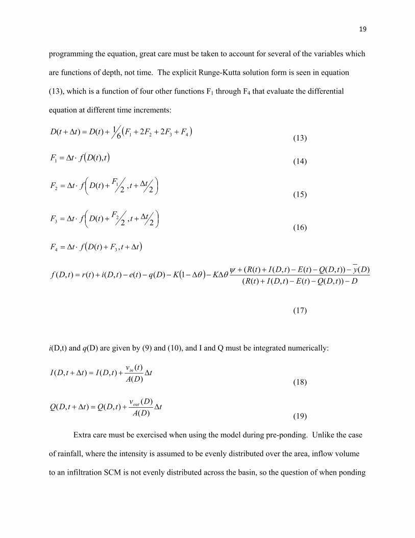
19
programming the equation, great care must be taken to account for several of the variables which
are functions of depth, not time. The explicit Runge-Kutta solution form is seen in equation
(13), which is a function of four other functions F1 through F4 that evaluate the differential
equation at different time increments:
( )4321 2261)()( FFFFtDttD ++++=Δ+
(13)
( )ttDftF ),(1 ⋅Δ= (14)
⎟⎠⎞⎜
⎝⎛ Δ++⋅Δ= 2,2)( 1
2ttFtDftF
(15)
⎟⎠⎞⎜
⎝⎛ Δ++⋅Δ= 2,2)( 2
3ttFtDftF
(16)
( )ttFtDftF Δ++⋅Δ= ,)( 34
( )DtDQtEtDItR
DytDQtEtDItRKKDqtetDitrtDf−−−+−−−++
Δ−Δ−−−−+=)),()(),()((
)()),()(),()((1)()(),()(),( ψθθ
(17)
i(D,t) and q(D) are given by (9) and (10), and I and Q must be integrated numerically:
tDAtv
tDIttDI in Δ+=Δ+)()(
),(),( (18)
tDADv
tDQttDQ out Δ+=Δ+)()(
),(),( (19)
Extra care must be exercised when using the model during pre-ponding. Unlike the case
of rainfall, where the intensity is assumed to be evenly distributed over the area, inflow volume
to an infiltration SCM is not evenly distributed across the basin, so the question of when ponding

20
begins is more difficult to answer. The area function – A(D) – is an important part of this
question. The assumption contained within equation (7) is that the inflow water is deposited
directly into the deepest point of the basin. In some cases, this might be true, but in many cases,
the water may flow over some soil before it gets to the bottom of the pond. If the latter case is
true, then the former case – the assumption in the model – will be a conservative estimate,
because water flowing over soil to get into the pond will infiltrate more than water directly
deposited at the bottom. When the depth is zero, equation (7) requires evaluation of the term
vin/A(D): the inflow volume expressed as a depth over the pond bottom. Therefore, the area
function at depth equal to zero must not be zero, but must be some finite area over which the
inflow water is deposited prior to ponding. In general, this may be difficult to determine
precisely, but will not be very important for low conductivity soils or high inflow rates where
ponding is likely to occur quickly. In other words, the user must assume that the pond area has a
small “flat bottom” area.
Finally, equation (7) is derived so that during pre-ponding, the depth at time t+Δt will be
a negative solution, indicating that the infiltration capacity is higher than the water available for
infiltration. Therefore, an “if” statement must be included in the model to reset the depth at time
t+Δt to zero if the solution is negative, before moving on to the next time step. As long as the
area function at negative depth equals the area function at depth equal to zero, this step will not
violate the conservation of mass.

21
4.3. Temperature Dependence
The temperature dependence of infiltration comes from the properties of water: viscosity
and density are temperature dependent properties. The definition of the hydraulic conductivity
is:
μρκ gK =
(20)
Where κ is the intrinsic permeability of the soil (temperature independent), ρ is the mass density
of water (varies with temperature, though negligibly for atmospheric temperatures), g is the
acceleration due to gravity, and µ is the viscosity of water, from which the temperature
dependence of K arises. A functional form for expansion of this temperature dependence around
20o C is given by Fogel’son and Likhachev (2001):
1408.247
29 10105.3)( −− ×⎟
⎠⎞
⎜⎝⎛ ⋅
×≈ T
inslbTμ
(21)
With T in Kelvin. The published values for hydraulic conductivity will generally be given at 20o
C. Using that information, the user can solve for the intrinsic permeability, and then use the
temperature dependent form of the equation.
4.4. Layered Soils
Often, infiltration basins are constructed with an engineered soil mixture near the surface
to allow for faster infiltration of water or to allow better growth of plants, or both. There are two
possibilities when dealing with layered soil that must be treated differently: the first will
generally be the most common, when the upper soil zone is higher hydraulic conductivity than

22
the lower, native soil; and the second is when the upper soil zone is lower conductivity than the
lower soil.
When the hydraulic conductivity decreases with increasing depth, the treatment of the
soil zones in the model is trivial. The assumption that must be made is that initially, the matric
suction is the same for each soil zone. This is a fair assumption (as fair as for one soil zone,
anyway), as a gradient in matric suction would result in flow of water until the gradient is gone.
In this case, there is no modification needed to the model other than to keep track of the
infiltrated water depth (F/Δθ), and when that depth exceeds the soil layer depth, then K and Δθ
must be switched to the values of the new soil. This works because the lower conductivity soil
will drive the infiltration rate; once the water column reaches the low conductivity soil, the
infiltration rate will be the same as if the entire soil thickness were the low conductivity soil. In
fact, it is trivial to add as many soil zones as needed, as long as the conductivity decreases with
each zone going down.
The second possibility is that the upper soil zone has a lower conductivity than the soil
beneath it. This is more difficult to model and in fact, the model assumption of having a sharp
wetting front will break down at this point. When the infiltrating water column reaches the
higher conductivity soil, the entire water column cannot speed up because the top part of the
column is limited by the low conductivity soil above. Thus, only the amount of water that leaves
the first soil zone will enter the higher conductivity zone and so that amount of water will begin
to infiltrate away faster than the rest of the column, breaking up the sharp wetting front. Within
the framework of this model, the result of entering the second soil zone would be that the
infiltrated water depth F would become constant (F/Δθ = depth of first soil zone), and as water
enters the soil below, it would become wetter (but not saturated), so the matric suction would

23
begin to decrease at an unknown rate. The only way of treating this scenario accurately would
be to use the Richards Equation, which is not easily solved in this scenario, would necessitate
knowledge of the second soil/water characteristic curve (K(θ)), and would also make a detailed
picture of the first curve (ψ(θ)) more critical. In other words, the full solution of this problem is
outside the scope of this model, because it would increase the computational power needed, and
decrease user-friendliness.
However, within the framework of the model, it is possible to bound the solution with an
upper and lower infiltration rate. At the upper end, assume that the conductivity of the lower soil
zone approaches infinity. In this case, the lower soil zone will act as an infinite reservoir for the
infiltrating water, and any water that enters it will be immediately “whisked away.” Thus, the
infiltrated water depth becomes constant (F/Δθ = depth of first soil zone), but the matric suction
would also remain constant because the water content would not increase. This is treated easily
within the model framework. At the lower end of infiltration rate, one could assume that there is
no change in soil type. In other words, adding the higher conductivity soil underneath cannot
slow the infiltration rate down from the case that all the soil had a lower conductivity. In many
cases, it is likely that the actual performance will be close to one or the other case; if the
conductivity of the two zones are similar, it will behave like the “lower end” case, and if the
second soil has an order of magnitude higher conductivity, then it will behave much like the
“upper end” case.
4.5. Green and Ampt Soil Parameters
The ponded infiltration model presented relies on the Green and Ampt infiltration
parameters K, ψ, and Δθ. Many tables are available for “typical” Green and Ampt values for the

24
USDA classification of soil types. However, these values may not necessarily be the most
appropriate values to use. In general, to solve the Richards equation, two soil/water
characteristic curves (SWCCs) are needed: K(θ) and ψ (θ) or K(ψ) and θ(ψ). One of the benefits
of using the Green and Ampt solution is that all of the infiltrating water is assumed to completely
saturate the soil, up to the sharp wetting front. For this reason, the conductivity SWCC (K(θ)) is
not needed, only the saturated hydraulic conductivity is needed. However, typical Green and
Ampt conductivities are about half the saturated hydraulic conductivity, owing to the unsaturated
soil beneath the wetting front having a small conductivity and from cyclical wetting conditions
creating air pockets in the soil. The practical implication is that Green and Ampt conductivities
are needed – not saturated hydraulic conductivities.
The remaining two parameters – ψ and Δθ – are often taken independently from tables as
well. Although the SWCC relating these two parameters is not needed to solve the equation, it is
often overlooked that these two parameters are related. For example, to study the effect of
changing ψ, it would not be appropriate to keep Δθ as a constant; doing so would create a set of
solutions that are not physically possible. Increasing ψ for a given soil will always correspond to
increased Δθ (the soil is drier), and vice-versa. Thus it is better to have either ψ or Δθ be the one
independent variable, and use the SWCC curve to determine the other. Fredlund (2006)
describes how using the SWCC in this way does not require great accuracy in the curve, as it
would in solving the Richards equation. This statement is confirmed later in the model
sensitivity studies. What this implies is that using one of the table SWCCs (e.g. Maulem - van
Genuchten values can be found in tables) will be sufficient for the model, but will be a large
improvement over having ψ and Δθ be separate independent variables. For this thesis, ψ will be

25
considered the independent variable rather than Δθ because its interpretation does not depend on
the soil type.
Ideally, for a model correlation, all three of the soil properties would be known for each
storm event. However, that is “easier said than done.” One reason is that the values for the
Green and Ampt model are averages over the entire basin, both area and depth. So, even if
several soil moisture probes were taking readings in the basin, it is unlikely that the data would
directly correspond to Δθ used in the equation. Similarly, taking a core sample of the soil and
doing a hydraulic conductivity test does not guarantee finding K for the Green and Ampt
equation. However, using available data at the site can yield information about the value for K:
it can be shown that the recession rate – dD/dt – decreases over time during any event, but its
magnitude will always be greater than or equal to K, under any circumstances (taking the limit of
equation (7) shows this). Therefore, a study of ponded recession limbs should provide an
estimate of K(T). As the initial moisture content approaches saturation, the infiltration rate more
closely approaches K. Therefore, it can be assumed that given enough data, some recession rates
will be quite close to K.
The typical recession limb of a depth versus time plot will be roughly linear. As such,
the average recession rate can be measured by performing a linear regression of the recession
limb. When the recession rates are plotted against temperature, there is a large variation at each
temperature, but the minimum recession rate increases with T with the same functional
dependence as K. Figure 4.2 demonstrates this principle with data from the Villanova traffic
island (VTI). The variation at each temperature is due to changes in storm size (more water
infiltrated will reduce the recession rate) and antecedent moisture conditions (initially wet soils
will have a lower recession rate). An assumption that must be made is that given enough events,
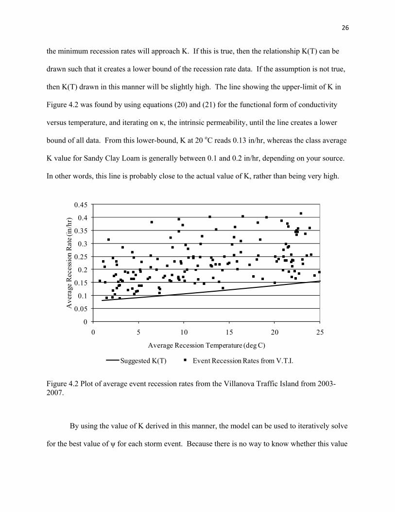
26
the minimum recession rates will approach K. If this is true, then the relationship K(T) can be
drawn such that it creates a lower bound of the recession rate data. If the assumption is not true,
then K(T) drawn in this manner will be slightly high. The line showing the upper-limit of K in
Figure 4.2 was found by using equations (20) and (21) for the functional form of conductivity
versus temperature, and iterating on κ, the intrinsic permeability, until the line creates a lower
bound of all data. From this lower-bound, K at 20 oC reads 0.13 in/hr, whereas the class average
K value for Sandy Clay Loam is generally between 0.1 and 0.2 in/hr, depending on your source.
In other words, this line is probably close to the actual value of K, rather than being very high.
Figure 4.2 Plot of average event recession rates from the Villanova Traffic Island from 2003-2007.
By using the value of K derived in this manner, the model can be used to iteratively solve
for the best value of ψ for each storm event. Because there is no way to know whether this value
0
0.05
0.1
0.15
0.2
0.25
0.3
0.35
0.4
0.45
0 5 10 15 20 25
Ave
rage
Rec
essi
on R
ate (
in/h
r)
Average Recession Temperature (deg C)
Suggested K(T) Event Recession Rates from V.T.I.

27
of K(T) is accurate, it can only be assumed as an upper limit. With an upper limit of K, all
values of ψ determined this way will be a lower limit. Thus, by knowing an upper bound of K,
the model can be used to determine a lower bound on ψ. This should yield some useful
information about the actual conditions in an infiltration basin, and thankfully, one of the sites at
Villanova University (VTI) has enough data to accomplish this. The other site, the Fedigan Rain
Garden (FRG), does not have enough data to do this, both because of time of operation and
because it has such a higher infiltration rate that it is rarely ponded.
4.6. Computational Methods
MATLAB was the software used to run these analyses. The model equations were
programmed with a 4th order Runge-Kutta explicit integration. The explicit integration uses
adaptive stepsize control (Press et al, 1988, Section 15.2): at each data timestep (5 minutes at
Villanova Traffic Island, 1 minute at Fedigan Rain Garden), the solution is performed at the data
timestep and half the data timestep. If the two solution pond depths differ by more than 10e-6,
then the new timestep is determined by equation (22):
0.90 10Δ
. (22)
For the model correlation studies, instead of depth being the primary unknown variable,
the initial matric suction is the primary unknown variable, and the depth is known (as a function
of time). However, the only way to solve the equation for ψ is iteratively. MATLAB comes
with an optimization routine that will find a least-squares solution for the error between model
depth and actual depth. The routine is “lsqnonlin” for least-squares nonlinear. This routine finds
the best-fit solution with as few iterations as possible.

28
4.7. Summary of Model Assumptions/Approximations
Several important assumptions and approximations are included in this model. Most
fundamentally, this is a one-dimensional infiltration model, and it assumes that the groundwater
table is at great depth. It is likely that the 1-D approximation is not valid if the saturated zone is
immediately beneath the soil surface. A shallow groundwater table also violates the assumptions
of the development of the hydraulic gradient in the Green and Ampt and Philip’s infiltration
models. Some other assumptions and approximations are:
• Soil hydraulic properties are homogenous over area and depth.
• The wetting front takes the shape of the wetted bowl surface. During recession, this will
cause the wetting front to become more curved than the bowl geometry over time.
• The wetting front is sharp, as in the Green and Ampt method.
• The initial matric suction is the same for all soil zones.

29
5. MODEL SENSITIVITIES
All of the working components of a model must be checked for sensitivity. If a part of
the model is very sensitive, then it requires an accurate knowledge of that parameter. If, on the
other hand, a parameter is very insensitive, then it can sometimes be eliminated entirely from the
model. The sensitivity must be evaluated in terms of uncertainty of model inputs, and how that
uncertainty affects the model outputs: in this case the primary model output is average
infiltration rate. The model inputs are the soil properties: the saturated hydraulic conductivity
(K), the initial matric suction (ψ), and the initial soil moisture content (θ) – as determined
through the soil water characteristic curve (SWCC); and the bowl shape.
The soil property sensitivity studies will be conducted with a hypothetical rain garden
that has the shape of a rectangular trough, where the bottom and top area are specified, and the
area in between is linear with respect to depth. This shape is such that the length to width ratio
does not affect any terms in the model. The rainfall and inflow hydrograph will be from a 0.99”
storm randomly selected from the Villanova traffic island data because of the round number.
The inflow volume from this event is 2275 ft3, and the bowl shape was picked to have a volume
of 2000 ft3 such that the bottom flat area is 500 ft2, the top area is 1500 ft2, and the height is 2 ft.
The soil conductivities are taken from Rawls et al (1992), and the SWCC is a van Genuchten
model parameterized with values taken from the USDA’s Rosetta model (Schaap 1999).
5.1. Hydraulic Conductivity Sensitivity
The saturated hydraulic conductivity (K) is expectedly an important/sensitive factor in
determining the infiltration rate. For this study, the baseline soil properties were that of a Sandy
Clay Loam (K = 0.118 in/hr), but a check was run with Loamy Sand (K = 2.406 in/hr) to ensure

30
that the results hold for all soil types. Sand would have even higher infiltration rates, but those
rates are so high that ponding is difficult to achieve with typical inflow rates. In each case, the
matric suction is about 80” – a value that is slightly lower (i.e. higher-moisture) than field
capacity (132”). Figure 5.1 shows the plot of several model runs where K is varied by a factor
between 0.5 and 2.0. The change in average recession rate is shown on the vertical axis. The
data plots a nearly straight line with a coefficient of 0.83, meaning that if K increases by 100%,
the average recession rate will increase by 83%. Thus, K is the most important model input.
This also shows the importance of including the temperature variability of K: a 10 degree Celsius
change in temperature will result in about a 25-30% change in K, which in turn will produce a
20-25% change in recession rate per 10 degrees.
Figure 5.1 Plot of change in conductivity (K) vs. change in average recession rate (RR).
5.2. Matric Suction Sensitivity
The matric suction is the only variable input parameter in the model. The conductivity
may vary with temperature, but the matric suction can vary based on the user’s discretion, as it is
y = 0.8272x + 0.1825R² = 0.9992
0
0.2
0.4
0.6
0.8
1
1.2
1.4
1.6
1.8
2
0 0.5 1 1.5 2 2.5
(Average
RR)/(Baseline Average
RR)
K/(Baseline K)
Sandy Clay Loam
Loamy Sand
Linear Fit (Sandy Clay Loam)

31
dependent on many factors, including antecedent weather and dry time, although a clear
relationship has not been discovered. Perhaps, a soil moisture accounting model would be able
to get close to predicting the matric suction. Note that as the matric suction changes, the initial
soil moisture content also changes, but the relationship is fixed (via the soil water characteristic
curve). The sensitivity of that relationship will be considered in Section 5.3. As with the
hydraulic conductivity, the sensitivity of the matric suction will be evaluated primarily with
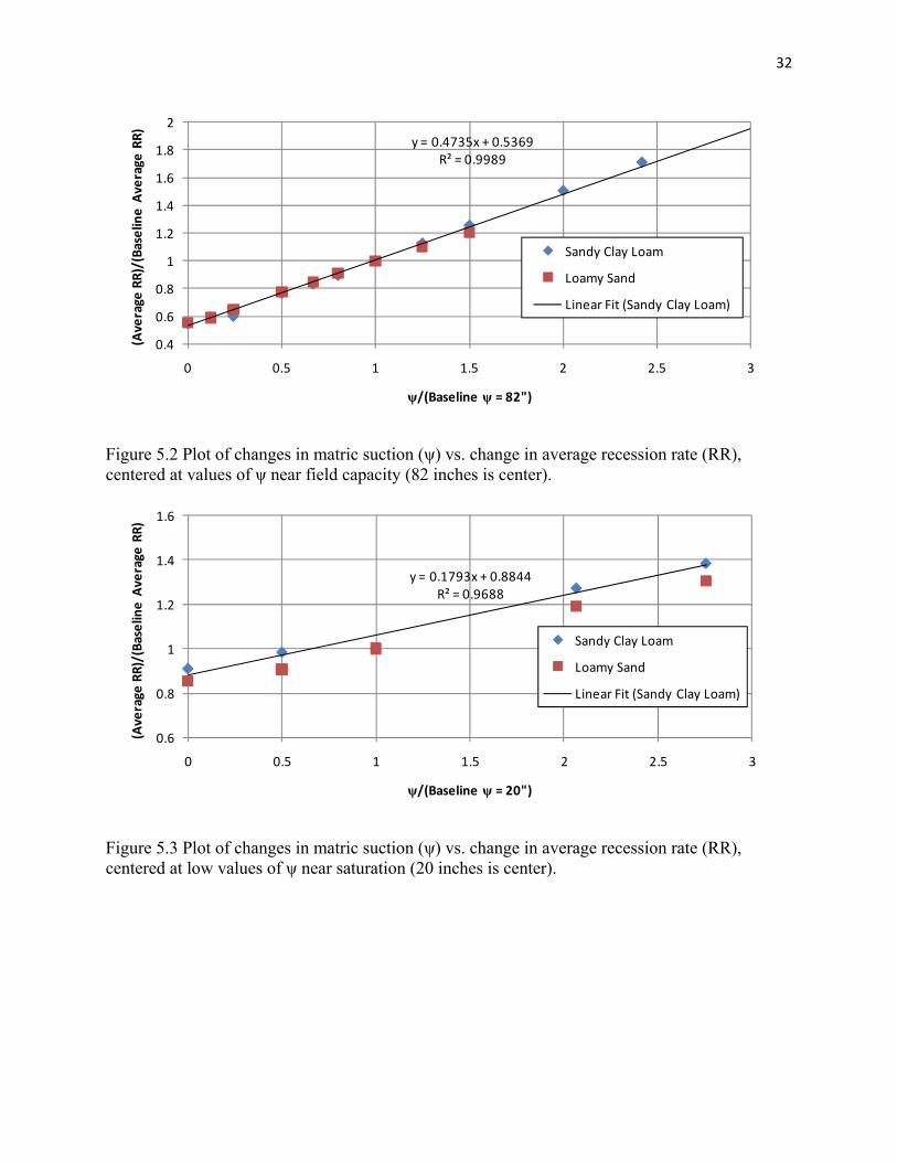
sandy clay loam, and then verified with loamy sand. Figure 5.2 shows the plot of several model
runs where ψ is varied from the “baseline” run of 82 inches – a number that is simply used as a
reference point. The change in average recession rate (relative to the baseline) is shown on the
vertical axis. The data plots a strong correlation with a linear coefficient of 0.47, meaning that if
ψ increases by 100%, the average recession rate will increase by 47%. This makes ψ an
important parameter in determining the infiltration rate, but is also not so dominant that some
uncertainty will completely undermine the results of the model run. Figure 5.3 is the same plot,
though re-centered around a lower suction value, 20 inches. This plot shows that for lower
values of suction (higher moisture content), the sensitivity is lower, with a coefficient of 0.18
rather than 0.47. This is good for a design engineer, who might wish to use the model
conservatively (i.e. with wet initial conditions). Thus, a conservative solution can be reached
without much sensitivity to suction, so one might decide to use a value from a Green and Ampt
parameter table, which tend to be low suction values.
32
Figure 5.2 Plot of changes in matric suction (ψ) vs. change in average recession rate (RR), centered at values of ψ near field capacity (82 inches is center).
Figure 5.3 Plot of changes in matric suction (ψ) vs. change in average recession rate (RR), centered at low values of ψ near saturation (20 inches is center).
y = 0.4735x + 0.5369R² = 0.9989
0.4
0.6
0.8
1
1.2
1.4
1.6
1.8
2
0 0.5 1 1.5 2 2.5 3
(Average
RR)/(Baseline Average
RR)
ψ/(Baseline ψ = 82")
Sandy Clay Loam
Loamy Sand
Linear Fit (Sandy Clay Loam)
y = 0.1793x + 0.8844R² = 0.9688
0.6
0.8
1
1.2
1.4
1.6
0 0.5 1 1.5 2 2.5 3
(Average
RR)/(Baseline Average
RR)
ψ/(Baseline ψ = 20")
Sandy Clay Loam
Loamy Sand
Linear Fit (Sandy Clay Loam)

33
5.3. Soil/Water Characteristic Curve Sensitivity
There are a wide range of soil water characteristic curves (SWCC), and every soil will be
different. The curve enables one to determine the value of soil moisture content (θ) given the
matric suction (ψ), or vice-versa. Because the curve is not linear, the effect of changes in the
curve must be evaluated at different values. For this study, the SWCC is modeled with the van
Genuchten (1980) form of the equation:
[ ] nn
rsr 11)(1
)(−
+
−+=
αψ
θθθψθ (23)
There are four model parameters: θr, θs, α, and n, which are the residual soil moisture, the
saturated soil moisture, and two curve-fitting parameters, respectively. Tables are available to
parameterize this equation with soil class average values. Generally, a standard deviation is
provided with the value, which can result in a very wide range for each parameter. In order to
get an understanding of the sensitivity, the model will be run with the equation from “adjacent”
soil types (adjacent in this case means the soil class with the closest value of hydraulic
conductivity, not the soil class with the closest grain-size distribution), rather than trying to apply
a Monte Carlo approach using the given standard deviations. In the latter case, there is no
guarantee that the values follow a normal distribution, and additionally it is almost certain that
the model parameters do not vary independently. Therefore, a Monte Carlo approach would
probably not be an accurate representation of SWCCs from that soil type.
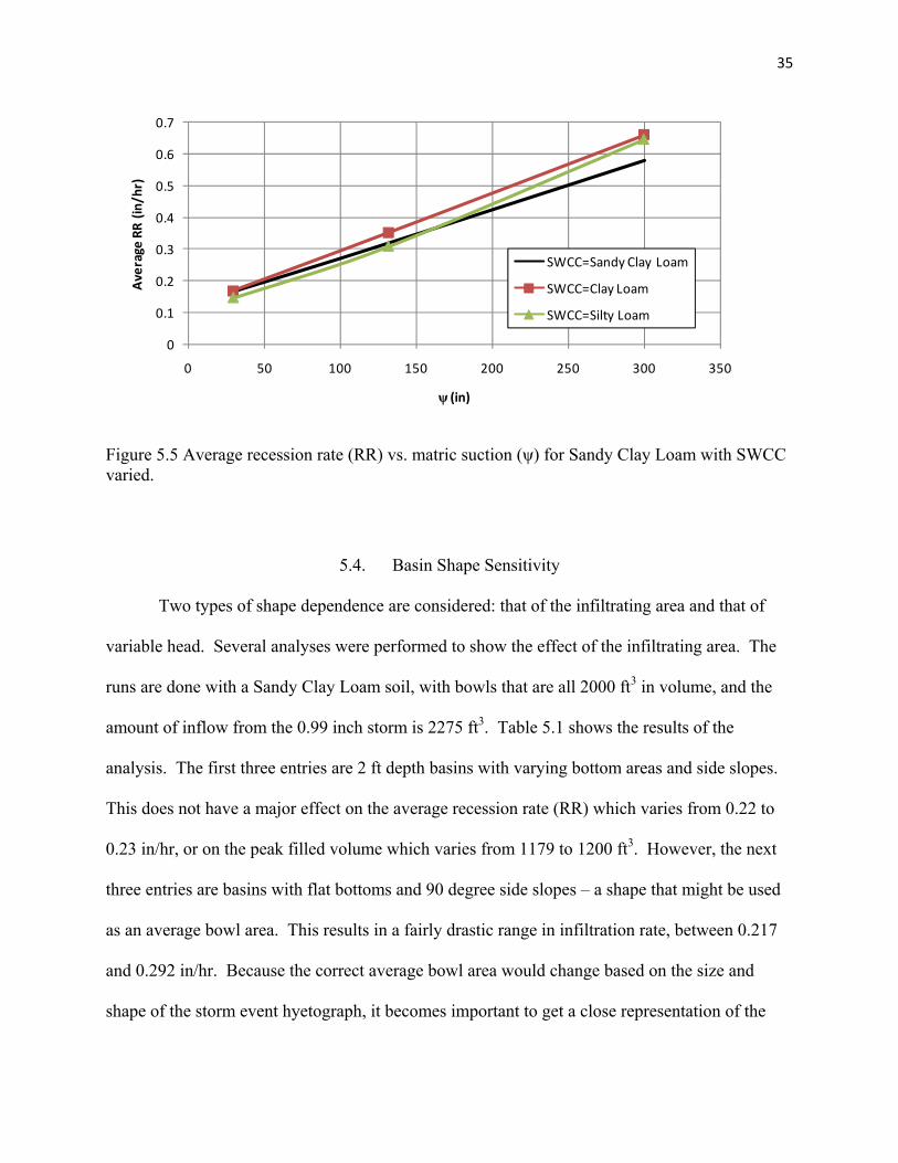
Figures 5.4 and 5.5 are plots of average recession rate vs. matric suction for Loamy Sand
(LS) and Sandy Clay Loam (SCL), respectively. For the LS analysis, the hydraulic conductivity
is held constant while the SWCC is changed to the mean values for Sand (S) and Sandy Loam
(Sa. L), which are the two closest soil classes in terms of hydraulic conductivity. For the similar
SCL analysis, the SWCC is changed to Silt Loam (Si. L) and Clay Loam (CL), again the closest

34
classes for conductivity. It can be seen that there are no major deviations from changing the
SWCC. The biggest change in RR was 13% at the highest values of ψ (300 inches) for the SCL,
but the rest of the curves for SCL and LS were within 10% of the baseline. This implies that the
SWCC is not particularly sensitive for this kind of analysis, which is a good thing for a design
engineer who will likely not have a SWCC tested for their soil, but who may use a grain-size
distribution based Pedo-transfer function to compute the SWCC (e.g. Fredlund et al, 2002). If
one were to do a complete Richard’s equation solution rather than the Philip’s solution, it is
highly likely that the SWCCs (there would be two curves – one for ψ and one for K) would be
more sensitive (Fredlund 2006); for practical purposes it is well that the SWCC has a low
sensitivity. Changes in the SWCC will also affect infiltration in multiple soil zones – changes in
θ affect the available pore space, thus affecting the timing of the infiltrating water hitting a
second soil zone.
Figure 5.4 Average recession rate (RR) vs. matric suction (ψ) for Loamy Sane with SWCC varied.
0
1
2
3
4
5
6
7
8
0 50 100 150 200 250 300 350
Average
RR (in
/hr)
ψ (in)
SWCC=Loamy Sand
SWCC=Sand
SWCC=Sandy Loam
35
Figure 5.5 Average recession rate (RR) vs. matric suction (ψ) for Sandy Clay Loam with SWCC varied.
5.4. Basin Shape Sensitivity
Two types of shape dependence are considered: that of the infiltrating area and that of
variable head. Several analyses were performed to show the effect of the infiltrating area. The
runs are done with a Sandy Clay Loam soil, with bowls that are all 2000 ft3 in volume, and the
amount of inflow from the 0.99 inch storm is 2275 ft3. Table 5.1 shows the results of the
analysis. The first three entries are 2 ft depth basins with varying bottom areas and side slopes.
This does not have a major effect on the average recession rate (RR) which varies from 0.22 to
0.23 in/hr, or on the peak filled volume which varies from 1179 to 1200 ft3. However, the next
three entries are basins with flat bottoms and 90 degree side slopes – a shape that might be used
as an average bowl area. This results in a fairly drastic range in infiltration rate, between 0.217
and 0.292 in/hr. Because the correct average bowl area would change based on the size and
shape of the storm event hyetograph, it becomes important to get a close representation of the
0
0.1
0.2
0.3
0.4
0.5
0.6
0.7
0 50 100 150 200 250 300 350
Average
RR (in
/hr)
ψ (in)
SWCC=Sandy Clay Loam
SWCC=Clay Loam
SWCC=Silty Loam
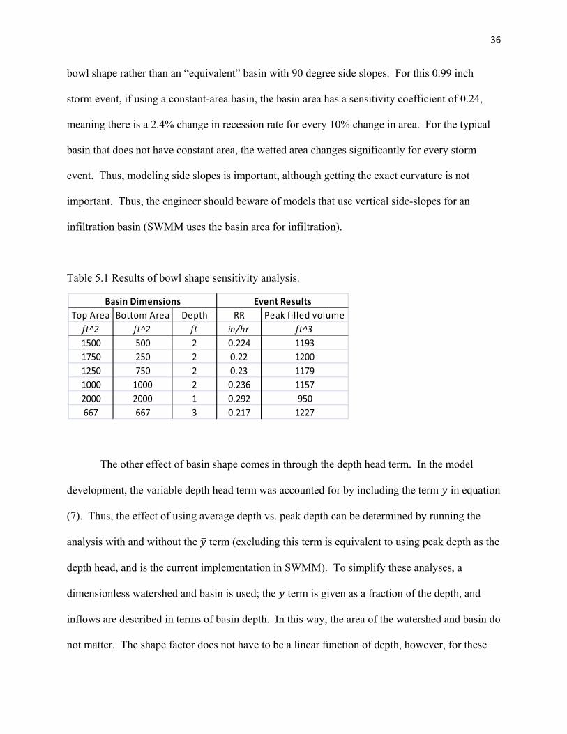
36
bowl shape rather than an “equivalent” basin with 90 degree side slopes. For this 0.99 inch
storm event, if using a constant-area basin, the basin area has a sensitivity coefficient of 0.24,
meaning there is a 2.4% change in recession rate for every 10% change in area. For the typical
basin that does not have constant area, the wetted area changes significantly for every storm
event. Thus, modeling side slopes is important, although getting the exact curvature is not
important. Thus, the engineer should beware of models that use vertical side-slopes for an
infiltration basin (SWMM uses the basin area for infiltration).
Table 5.1 Results of bowl shape sensitivity analysis.
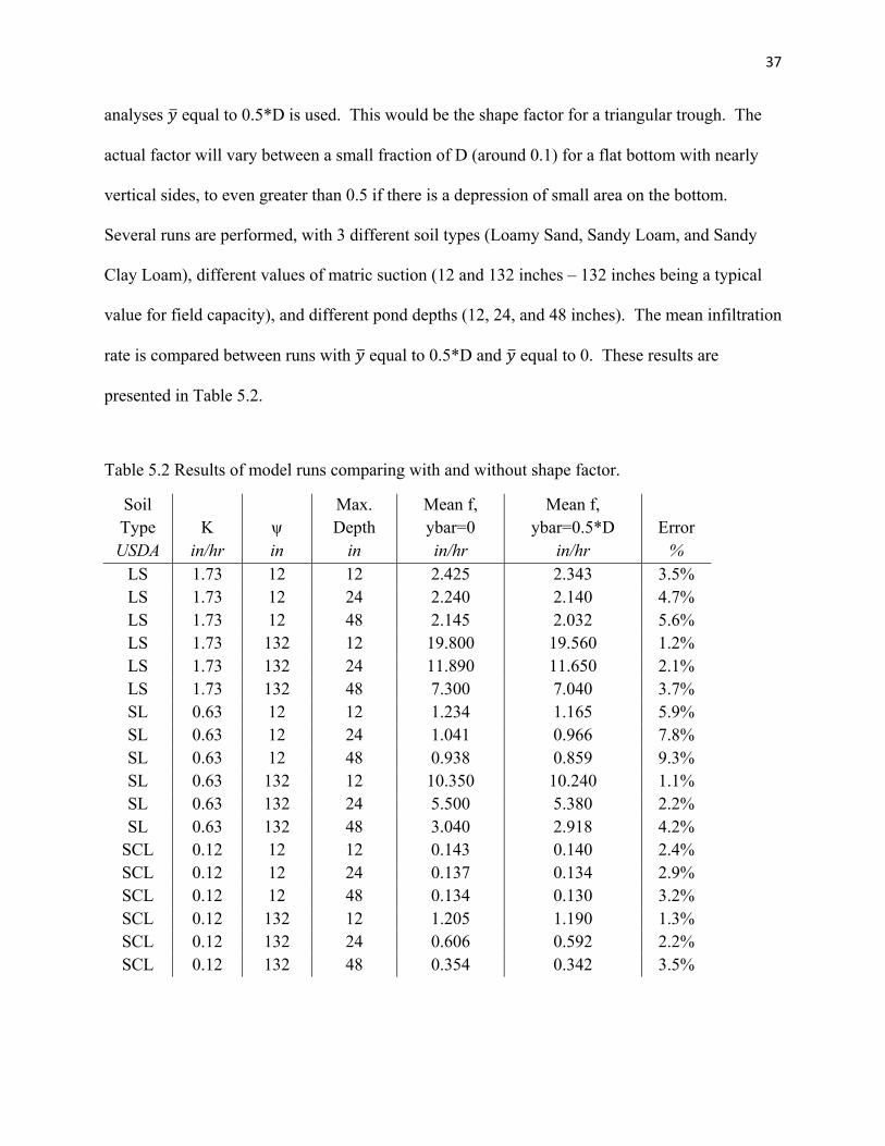
The other effect of basin shape comes in through the depth head term. In the model
development, the variable depth head term was accounted for by including the term in equation
(7). Thus, the effect of using average depth vs. peak depth can be determined by running the
analysis with and without the term (excluding this term is equivalent to using peak depth as the
depth head, and is the current implementation in SWMM). To simplify these analyses, a
dimensionless watershed and basin is used; the term is given as a fraction of the depth, and
inflows are described in terms of basin depth. In this way, the area of the watershed and basin do
not matter. The shape factor does not have to be a linear function of depth, however, for these
Top Area Bottom Area Depth RR Peak filled volumeft^2 ft^2 ft in/hr ft^31500 500 2 0.224 11931750 250 2 0.22 12001250 750 2 0.23 11791000 1000 2 0.236 11572000 2000 1 0.292 950667 667 3 0.217 1227
Basin Dimensions Event Results
37
analyses equal to 0.5*D is used. This would be the shape factor for a triangular trough. The
actual factor will vary between a small fraction of D (around 0.1) for a flat bottom with nearly
vertical sides, to even greater than 0.5 if there is a depression of small area on the bottom.
Several runs are performed, with 3 different soil types (Loamy Sand, Sandy Loam, and Sandy
Clay Loam), different values of matric suction (12 and 132 inches – 132 inches being a typical
value for field capacity), and different pond depths (12, 24, and 48 inches). The mean infiltration
rate is compared between runs with equal to 0.5*D and equal to 0. These results are
presented in Table 5.2.
Table 5.2 Results of model runs comparing with and without shape factor.
Soil Type K ψ
Max. Depth
Mean f, ybar=0
Mean f, ybar=0.5*D Error
USDA in/hr in in in/hr in/hr % LS 1.73 12 12 2.425 2.343 3.5% LS 1.73 12 24 2.240 2.140 4.7% LS 1.73 12 48 2.145 2.032 5.6% LS 1.73 132 12 19.800 19.560 1.2% LS 1.73 132 24 11.890 11.650 2.1% LS 1.73 132 48 7.300 7.040 3.7% SL 0.63 12 12 1.234 1.165 5.9% SL 0.63 12 24 1.041 0.966 7.8% SL 0.63 12 48 0.938 0.859 9.3% SL 0.63 132 12 10.350 10.240 1.1% SL 0.63 132 24 5.500 5.380 2.2% SL 0.63 132 48 3.040 2.918 4.2%
SCL 0.12 12 12 0.143 0.140 2.4% SCL 0.12 12 24 0.137 0.134 2.9% SCL 0.12 12 48 0.134 0.130 3.2% SCL 0.12 132 12 1.205 1.190 1.3% SCL 0.12 132 24 0.606 0.592 2.2% SCL 0.12 132 48 0.354 0.342 3.5%

38
Looking at the results of Table 5.2, a couple trends can be identified. First, the
importance of the shape factor is heavily dependent on pond depth. This makes sense because
will generally be an increasing function of depth, so more depth increases the importance of the
term. Also, the shape factor is sensitive to initial matric suction. It is most important when
matric suction is small (initially wet conditions) because is directly compared to ψ in the model
equation, so when ψ is smaller, is more important relatively. Finally, the results depend on the
soil type, but not in an obvious way. Sandy Loam was the most sensitive soil type, but its
conductivity is between Loamy Sand and Sandy Clay Loam. For many stormwater control
basins, ignoring the shape factor term may be acceptable, as error will be around 5% or less.
However, it might become important for large infiltration basins (>3 ft depth). Unfortunately,
leaving out this term (as in SWMM) is always un-conservative, since the mean depth is always
less than the peak depth. Although ignoring the variable depth is un-conservative, the error
associated is generally less than the uncertainty of other parameters such as conductivity and
matric suction.

39
6. MODEL APPLICATIONS
6.1. Villanova Traffic Island
6.1.1. Site Overview
The primary data set used for model calibration and verification will be from the
Villanova Traffic Island (VTI), seen in Figure 6.1. The VTI has been in operation since the end
of 2002, with a nearly continuous data record of rainfall and pond depth at 5 minute intervals.
The pond depth is measured using an ultrasonic distance sensor. A survey of the pond has been
performed to determine the geometry, which is necessary as a model input. Additionally, a soil
particle-size distribution test has been done (Isaac-Ricketts, 2008, and Gilbert Jenkins et al,
2010), which allows for a reliable estimation of the soil type. The primary limitations of this
data set are that soil moisture is not measured, and the inflow volumes are not measured.
Therefore, the inflow volumes must be estimated using the NRCS Curve Number method
(NRCS, 1993; Neitsch et al, 2005).
The traffic island has a total watershed area of 1.21 acres (0.5 acres of impervious
surface). The curve numbers used for this watershed are 98 for the impervious surface and 80
for the pervious surface. The infiltration basin itself has an area of 1550 ft2 (0.036 acres) and a
volume of 1270 ft3 when the depth is 1.72 ft at start of overflow. The traffic island was
constructed with 4 ft of engineered soil – native soil mixed with sand in a one-to-one ratio. In
this area of campus, there is a significant clay component (30%) near the soil surface, which
results in a Sandy Clay Loam type soil after mixing. However, at depth greater than 3 feet, the
clay component is reduced significantly to below 20% (Soil Survey Staff, 2011), meaning that

the soil u
discussed
this site a
suction v
Figure 6.
T
unknown
with the
underneath th
d in Section
at 0.13 in/hr.
values.
.1 Villanova
There is no of
n variable. S
depth vs. tim
he constructe
4.5, an uppe
. So, analys
a traffic islan
fficial “valid
So here, the m
me data. On
ed soil has a
er bound can
es run with t
nd while pon
6.1.2. M
dation” of th
model is run
e major prob
a higher cond
n be placed o
this conduct
nded.
Model Correl
he model bec
n iteratively o
blem with th
ductivity eve
on the Green
tivity will yie
lation
cause the init
on ψ until a
his correlatio
en than the m
n and Ampt c
eld a lower b
tial matric su
least-square
on is that the
mixed soil. A
conductivity
bound on ma
uction, ψ, is
es fit is achie
inflow
40
As
y for
atric
an
eved

41
hydrograph is not known, but predicted using the curve number method (98 for impervious
surface, 80 for pervious surface). Due to obvious discrepancies in the inflow volume, and also
because of missing data and freezing temperatures, several ponding events were excluded from
this correlation. There are a total of 66 events for the model correlation, between January 2003
and March 2008. These events are defined by ponding duration, so some of the events include
multiple distinct storm events. Qualitatively, the model is able to produce a good fit to the data
in all cases. Quantifying this is difficult because of uncertainties in the inflow volume and error
in the data (the depth sensors tend to fluctuate with temperature).
Figures 6.2 and 6.3 are two of the storm events (more are in Appendix A) that highlight
some important points of the model: Figure 6.2 shows a large storm event (actually three
successive storms, but close enough together that the pond does not empty) of 4.54 inches of
rain, and Figure 6.3 is a small event of only 0.35 inches of rain. The large event shows clearly
that the infiltration rate is constant; the infiltrating water has passed the constructed soil and
entered the higher-conductivity soil beneath. As discussed in the Methods section, this results in
a constant infiltration rate. The smaller event is one where the infiltration rate can be seen to be
decreasing over the recession limb. This is consistent with the infiltrating water column being all
within the same soil layer. At this site, the decreasing infiltration rate is only visible on a few
number of events; most events larger than 0.5 inches or so infiltrate through the engineered soil
before the inflow and rainfall cease.
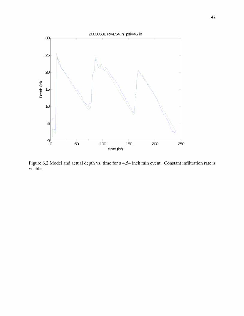
42
Figure 6.2 Model and actual depth vs. time for a 4.54 inch rain event. Constant infiltration rate is visible.
0 50 100 150 200 2500
5
10
15
20
25
3020030531 R=4.54 in psi=46 in
Dep
th (i
n)
time (hr)
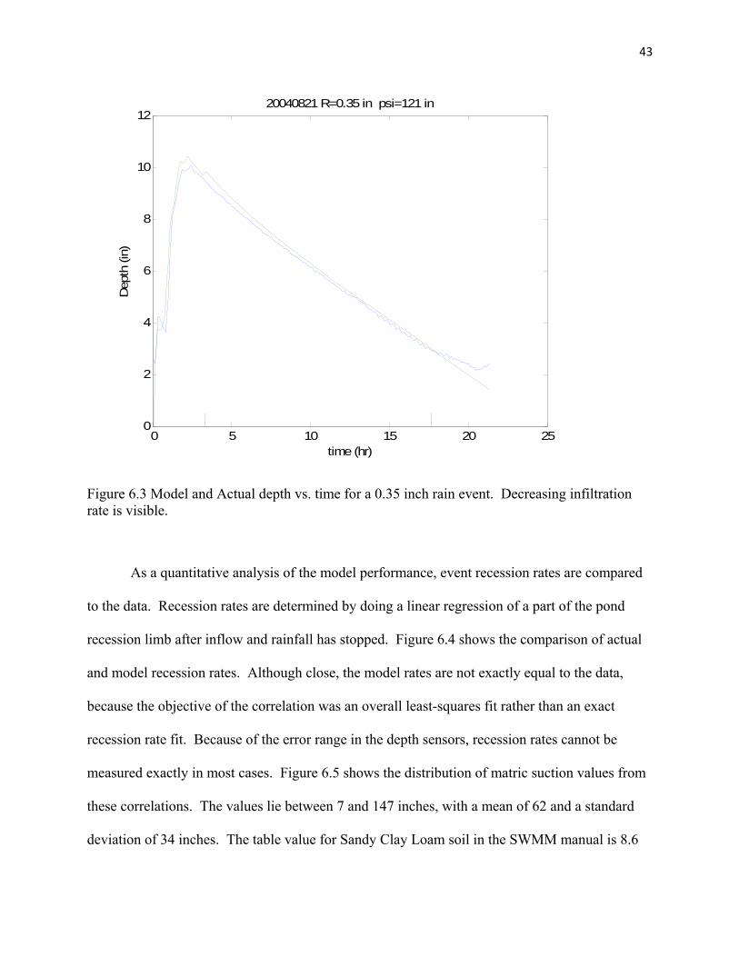
43
Figure 6.3 Model and Actual depth vs. time for a 0.35 inch rain event. Decreasing infiltration rate is visible.
As a quantitative analysis of the model performance, event recession rates are compared
to the data. Recession rates are determined by doing a linear regression of a part of the pond
recession limb after inflow and rainfall has stopped. Figure 6.4 shows the comparison of actual
and model recession rates. Although close, the model rates are not exactly equal to the data,
because the objective of the correlation was an overall least-squares fit rather than an exact
recession rate fit. Because of the error range in the depth sensors, recession rates cannot be
measured exactly in most cases. Figure 6.5 shows the distribution of matric suction values from
these correlations. The values lie between 7 and 147 inches, with a mean of 62 and a standard
deviation of 34 inches. The table value for Sandy Clay Loam soil in the SWMM manual is 8.6
0 5 10 15 20 250
2
4
6
8
10
1220040821 R=0.35 in psi=121 in
Dep
th (i
n)
time (hr)
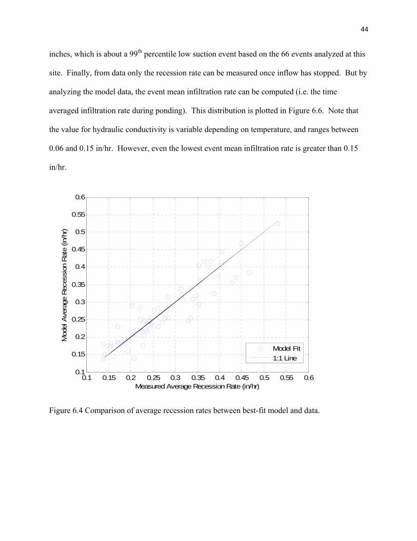
44
inches, which is about a 99th percentile low suction event based on the 66 events analyzed at this
site. Finally, from data only the recession rate can be measured once inflow has stopped. But by
analyzing the model data, the event mean infiltration rate can be computed (i.e. the time
averaged infiltration rate during ponding). This distribution is plotted in Figure 6.6. Note that
the value for hydraulic conductivity is variable depending on temperature, and ranges between
0.06 and 0.15 in/hr. However, even the lowest event mean infiltration rate is greater than 0.15
in/hr.
Figure 6.4 Comparison of average recession rates between best-fit model and data.
0.1 0.15 0.2 0.25 0.3 0.35 0.4 0.45 0.5 0.55 0.60.1
0.15
0.2
0.25
0.3
0.35
0.4
0.45
0.5
0.55
0.6
Measured Average Recession Rate (in/hr)
Mod
el A
vera
ge R
eces
sion
Rat
e (in
/hr)
Model Fit1:1 Line
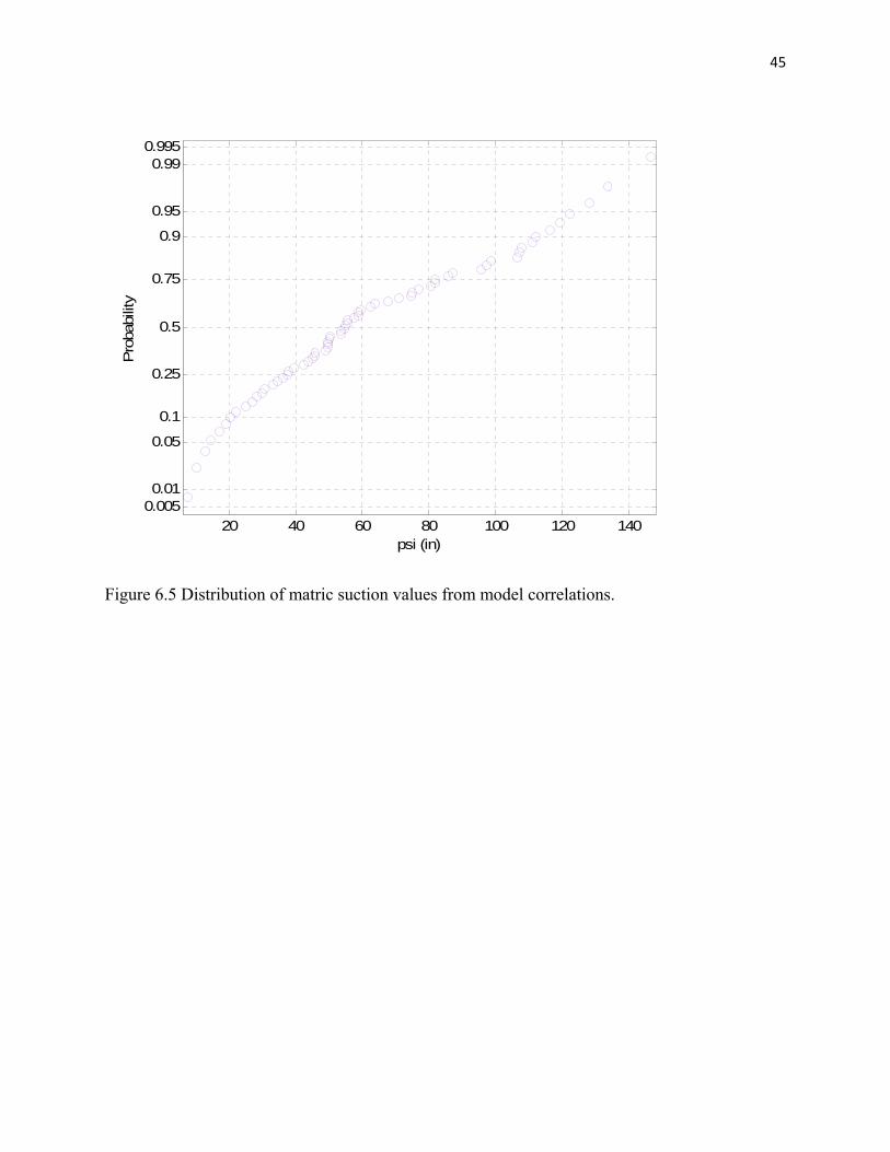
45
Figure 6.5 Distribution of matric suction values from model correlations.
20 40 60 80 100 120 1400.0050.01
0.05
0.1
0.25
0.5
0.75
0.9
0.95
0.990.995
psi (in)
Pro
babi
lity
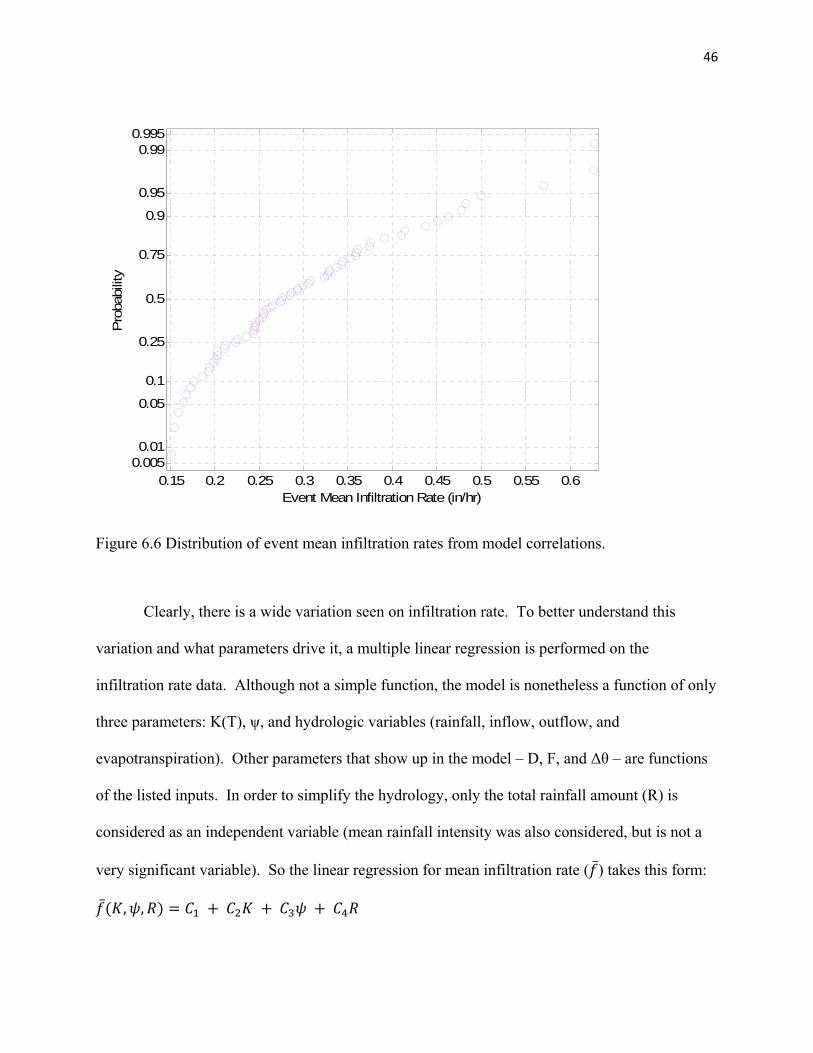
46
Figure 6.6 Distribution of event mean infiltration rates from model correlations.
Clearly, there is a wide variation seen on infiltration rate. To better understand this
variation and what parameters drive it, a multiple linear regression is performed on the
infiltration rate data. Although not a simple function, the model is nonetheless a function of only
three parameters: K(T), ψ, and hydrologic variables (rainfall, inflow, outflow, and
evapotranspiration). Other parameters that show up in the model – D, F, and Δθ – are functions
of the listed inputs. In order to simplify the hydrology, only the total rainfall amount (R) is
considered as an independent variable (mean rainfall intensity was also considered, but is not a
very significant variable). So the linear regression for mean infiltration rate ( ) takes this form:
, ,
0.15 0.2 0.25 0.3 0.35 0.4 0.45 0.5 0.55 0.60.0050.01
0.05
0.1
0.25
0.5
0.75
0.9
0.95
0.990.995
Event Mean Infiltration Rate (in/hr)
Pro
babi
lity
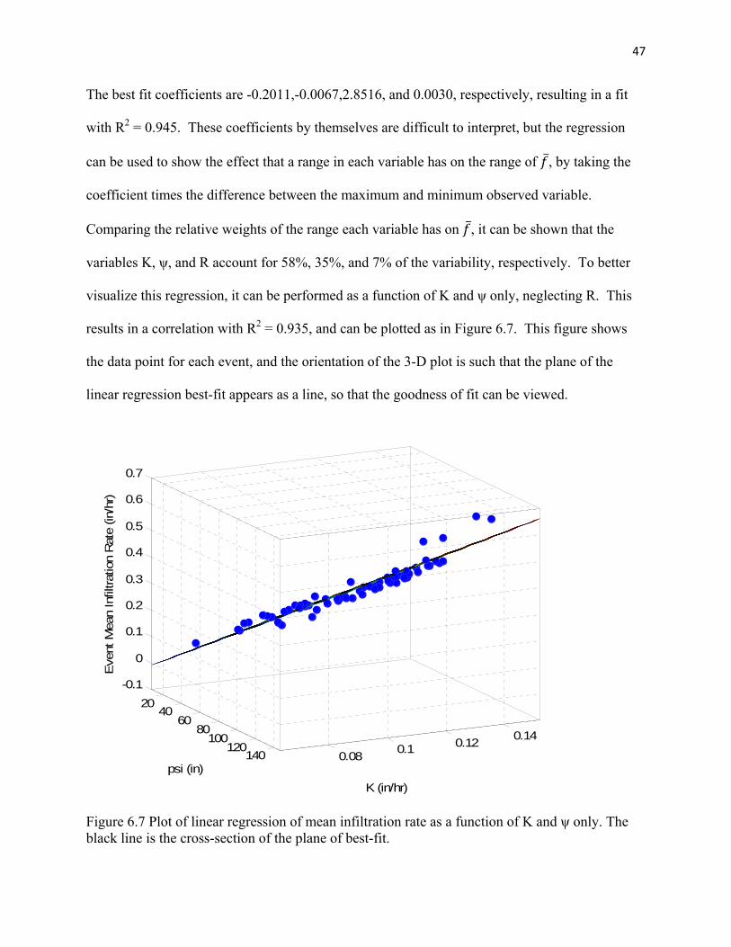
47
The best fit coefficients are -0.2011,-0.0067,2.8516, and 0.0030, respectively, resulting in a fit
with R2 = 0.945. These coefficients by themselves are difficult to interpret, but the regression
can be used to show the effect that a range in each variable has on the range of , by taking the
coefficient times the difference between the maximum and minimum observed variable.
Comparing the relative weights of the range each variable has on , it can be shown that the
variables K, ψ, and R account for 58%, 35%, and 7% of the variability, respectively. To better
visualize this regression, it can be performed as a function of K and ψ only, neglecting R. This
results in a correlation with R2 = 0.935, and can be plotted as in Figure 6.7. This figure shows
the data point for each event, and the orientation of the 3-D plot is such that the plane of the
linear regression best-fit appears as a line, so that the goodness of fit can be viewed.
Figure 6.7 Plot of linear regression of mean infiltration rate as a function of K and ψ only. The black line is the cross-section of the plane of best-fit.
0.08 0.1 0.12 0.14
2040
6080
100120
140
-0.1
0
0.1
0.2
0.3
0.4
0.5
0.6
0.7
K (in/hr)psi (in)
Eve
nt M
ean
Infil
tratio
n R
ate
(in/h
r)
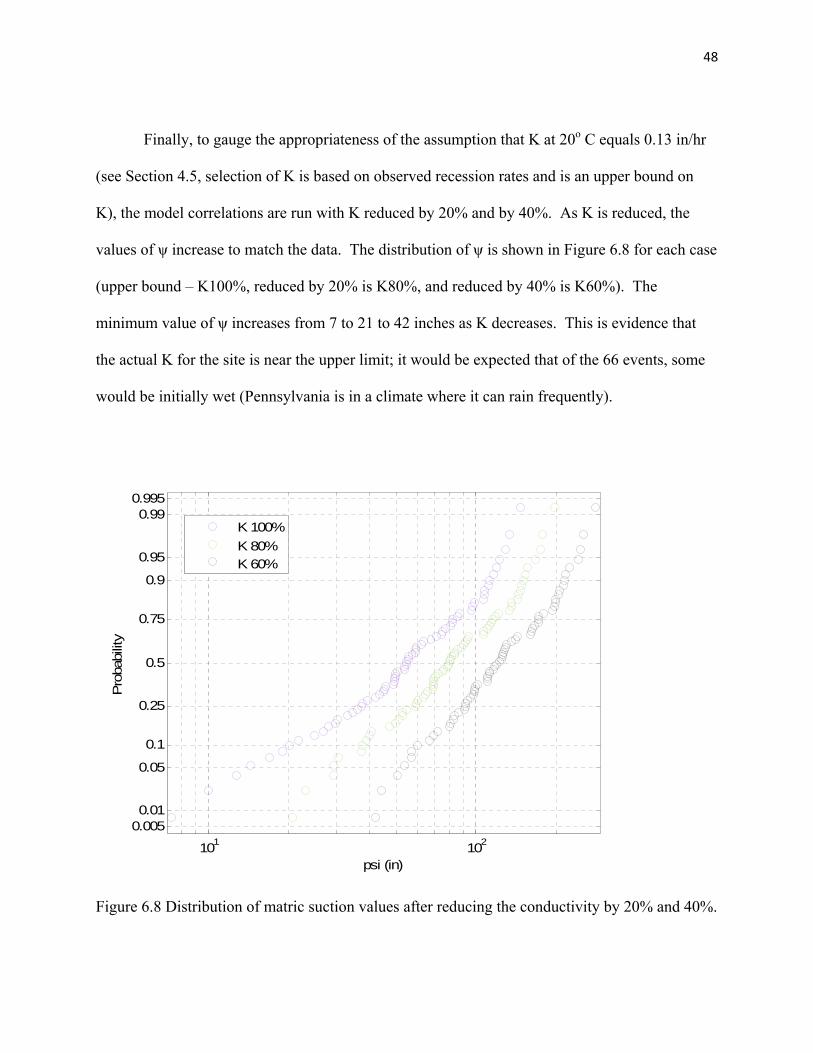
48
Finally, to gauge the appropriateness of the assumption that K at 20o C equals 0.13 in/hr
(see Section 4.5, selection of K is based on observed recession rates and is an upper bound on
K), the model correlations are run with K reduced by 20% and by 40%. As K is reduced, the
values of ψ increase to match the data. The distribution of ψ is shown in Figure 6.8 for each case
(upper bound – K100%, reduced by 20% is K80%, and reduced by 40% is K60%). The
minimum value of ψ increases from 7 to 21 to 42 inches as K decreases. This is evidence that
the actual K for the site is near the upper limit; it would be expected that of the 66 events, some
would be initially wet (Pennsylvania is in a climate where it can rain frequently).
Figure 6.8 Distribution of matric suction values after reducing the conductivity by 20% and 40%.
101 1020.0050.01
0.05
0.1
0.25
0.5
0.75
0.9
0.95
0.990.995
psi (in)
Pro
babi
lity
K 100%K 80%K 60%

49
6.2. Fedigan Rain Garden
6.2.1. Site Overview
The Fedigan Rain Garden (FRG), as seen in Figure 6.9, was recently built to capture the
runoff from the roof of the Fedigan building, a dormitory on Villanova University’s campus.
The area of roof captured is about 1700 ft2, and the area of the rain garden at start of overflow (1
ft depth) is about 750 ft2 with a storage volume of about 550 ft3. Unlike at the traffic island, no
site survey was performed, so only construction plans were used for dimensioning and soil
classification. The engineered soil is 1.5 feet deep, and is classified as USDA type Loamy Sand.
The native soil is Sandy Loam. At this site, inflow, pond depth, and outflow are measured using
pressure transducers. The inflow comes in through a 60 degree V-notch weir, and the overflow
goes through an 8 inch Thel-mar weir. Depths at the inflow weir, outflow weir, and in the pond
are measured using pressure transducers.
The FRG is considered a “verification” of the model rather than a “validation” because
there are so few storm events available for comparison, as the site is still under development.
During the data collection from August 2010 through November 2010, there were three events
with ponding recorded in the pond pressure transducer. Of these, only one had a significant
amount of ponding. For ponding less than an inch or so, the site data collection and setup is not
very accurate or reliable. The exact relationship between the pond bottom and the bottom of the
pressure transducer is not known, and the model assumption that there is a wide, perfectly flat
area will never be the case in reality. Those small variations in the actual pond bottom make
correlating to small pond depths difficult. This would be a measurement limitation at any site
with shallow ponding and a “natural” bottom.
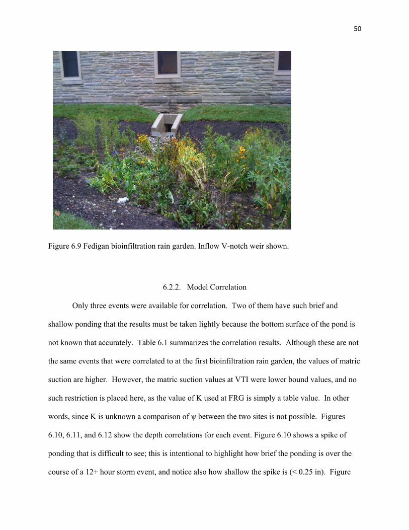
50
Figure 6.9 Fedigan bioinfiltration rain garden. Inflow V-notch weir shown.
6.2.2. Model Correlation
Only three events were available for correlation. Two of them have such brief and
shallow ponding that the results must be taken lightly because the bottom surface of the pond is
not known that accurately. Table 6.1 summarizes the correlation results. Although these are not
the same events that were correlated to at the first bioinfiltration rain garden, the values of matric
suction are higher. However, the matric suction values at VTI were lower bound values, and no
such restriction is placed here, as the value of K used at FRG is simply a table value. In other
words, since K is unknown a comparison of ψ between the two sites is not possible. Figures
6.10, 6.11, and 6.12 show the depth correlations for each event. Figure 6.10 shows a spike of
ponding that is difficult to see; this is intentional to highlight how brief the ponding is over the
course of a 12+ hour storm event, and notice also how shallow the spike is (< 0.25 in). Figure
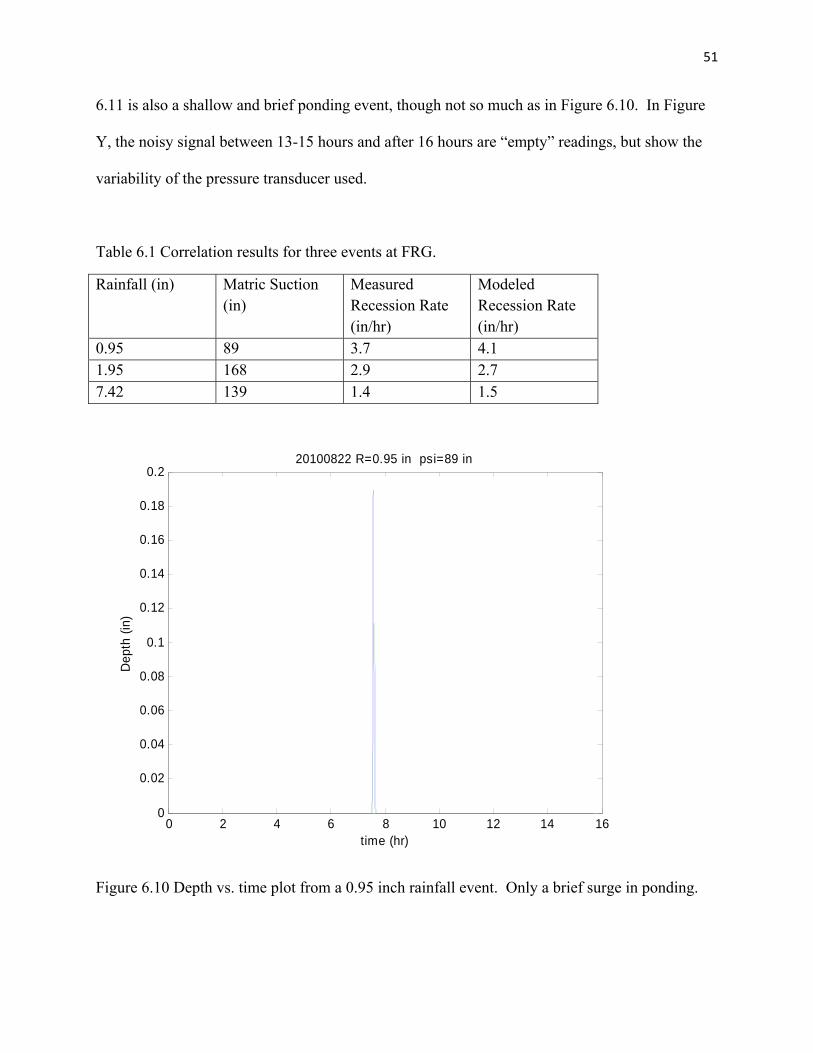
51
6.11 is also a shallow and brief ponding event, though not so much as in Figure 6.10. In Figure
Y, the noisy signal between 13-15 hours and after 16 hours are “empty” readings, but show the
variability of the pressure transducer used.
Table 6.1 Correlation results for three events at FRG.
Rainfall (in) Matric Suction (in)
Measured Recession Rate (in/hr)
Modeled Recession Rate (in/hr)
0.95 89 3.7 4.1 1.95 168 2.9 2.7 7.42 139 1.4 1.5
Figure 6.10 Depth vs. time plot from a 0.95 inch rainfall event. Only a brief surge in ponding.
0 2 4 6 8 10 12 14 160
0.02
0.04
0.06
0.08
0.1
0.12
0.14
0.16
0.18
0.220100822 R=0.95 in psi=89 in
Dep
th (i
n)
time (hr)
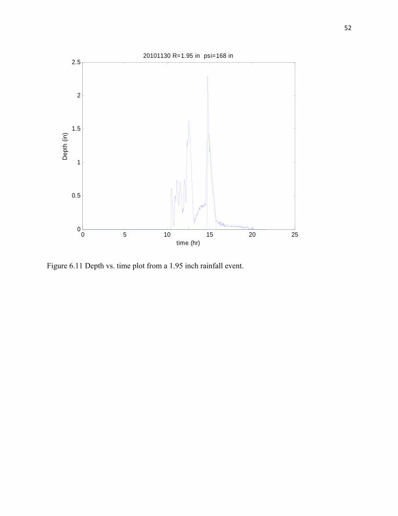
52
Figure 6.11 Depth vs. time plot from a 1.95 inch rainfall event.
0 5 10 15 20 250
0.5
1
1.5
2
2.520101130 R=1.95 in psi=168 in
Dep
th (i
n)
time (hr)
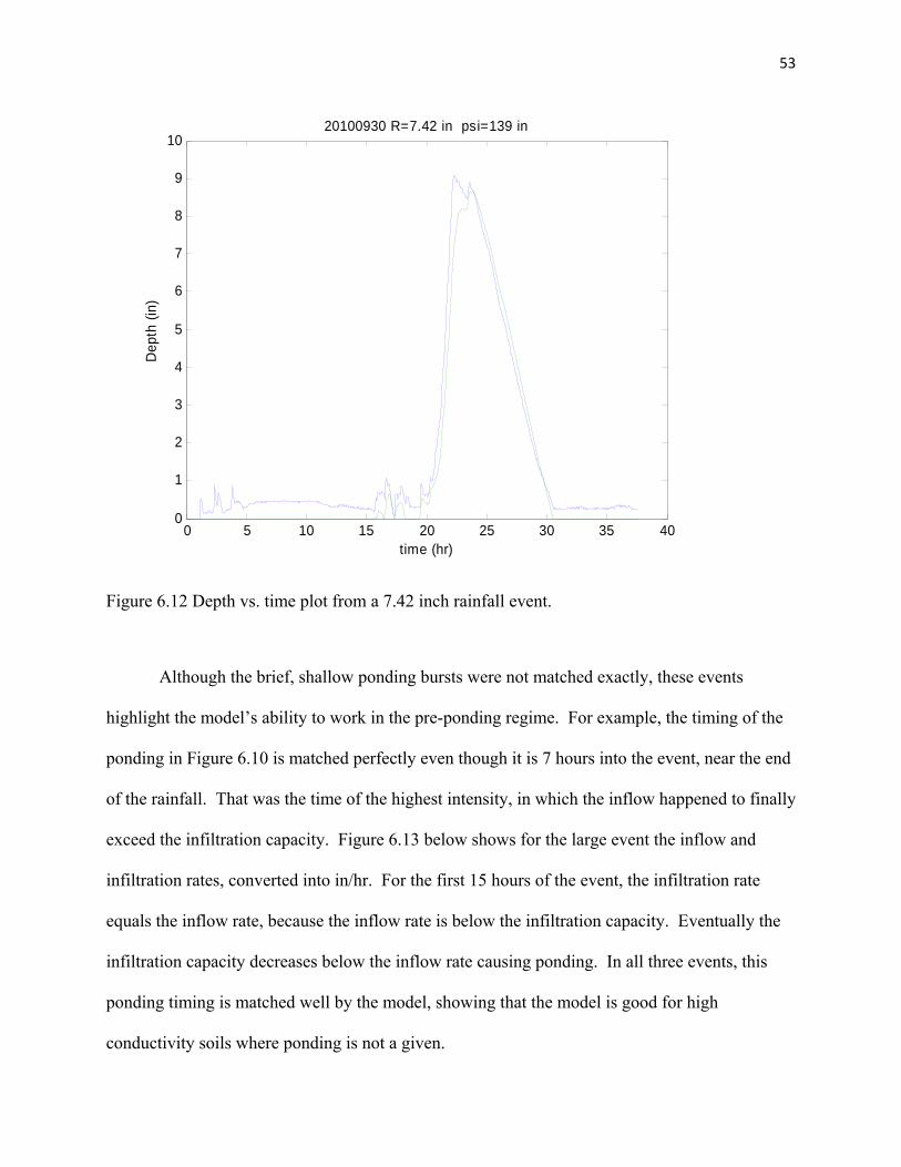
53
Figure 6.12 Depth vs. time plot from a 7.42 inch rainfall event.
Although the brief, shallow ponding bursts were not matched exactly, these events
highlight the model’s ability to work in the pre-ponding regime. For example, the timing of the
ponding in Figure 6.10 is matched perfectly even though it is 7 hours into the event, near the end
of the rainfall. That was the time of the highest intensity, in which the inflow happened to finally
exceed the infiltration capacity. Figure 6.13 below shows for the large event the inflow and
infiltration rates, converted into in/hr. For the first 15 hours of the event, the infiltration rate
equals the inflow rate, because the inflow rate is below the infiltration capacity. Eventually the
infiltration capacity decreases below the inflow rate causing ponding. In all three events, this
ponding timing is matched well by the model, showing that the model is good for high
conductivity soils where ponding is not a given.
0 5 10 15 20 25 30 35 400
1
2
3
4
5
6
7
8
9
1020100930 R=7.42 in psi=139 in
Dep
th (i
n)
time (hr)
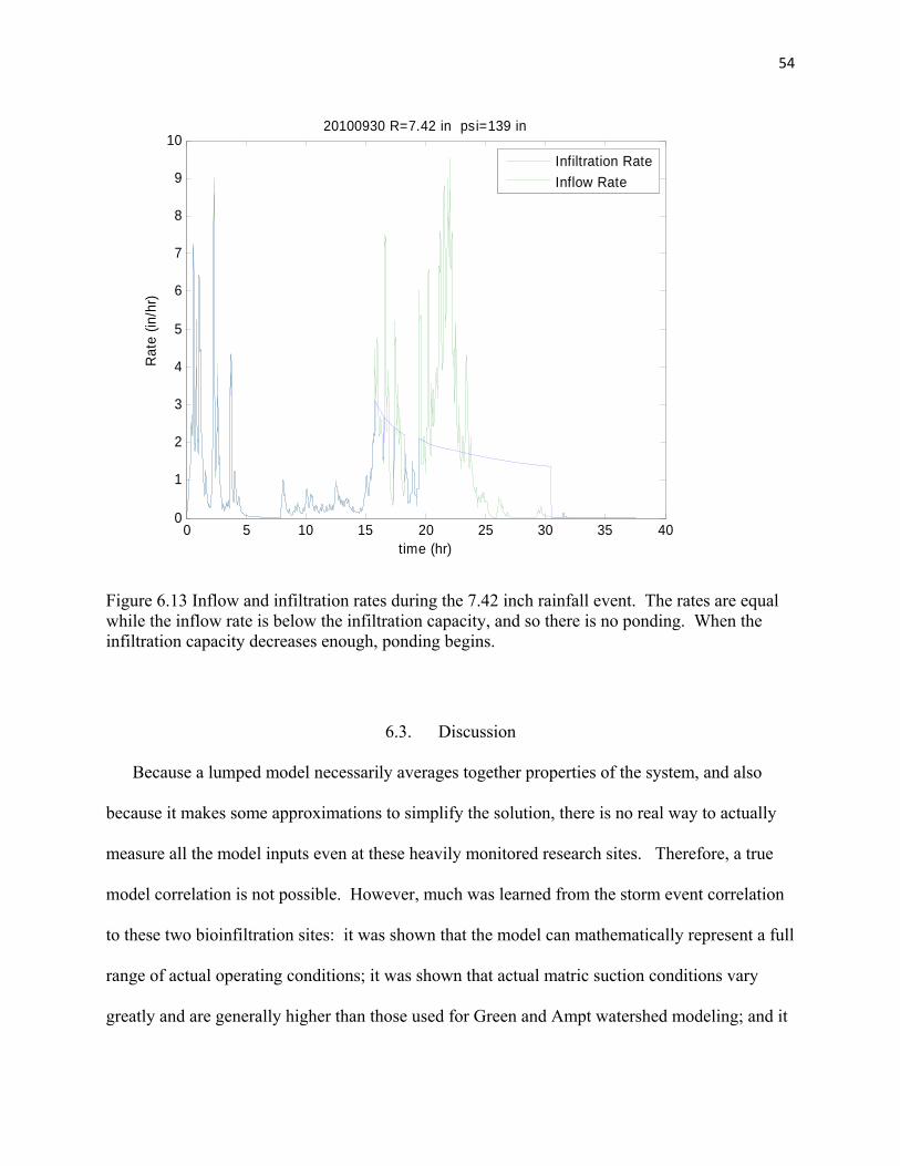
54
Figure 6.13 Inflow and infiltration rates during the 7.42 inch rainfall event. The rates are equal while the inflow rate is below the infiltration capacity, and so there is no ponding. When the infiltration capacity decreases enough, ponding begins.
6.3. Discussion
Because a lumped model necessarily averages together properties of the system, and also
because it makes some approximations to simplify the solution, there is no real way to actually
measure all the model inputs even at these heavily monitored research sites. Therefore, a true
model correlation is not possible. However, much was learned from the storm event correlation
to these two bioinfiltration sites: it was shown that the model can mathematically represent a full
range of actual operating conditions; it was shown that actual matric suction conditions vary
greatly and are generally higher than those used for Green and Ampt watershed modeling; and it
0 5 10 15 20 25 30 35 400
1
2
3
4
5
6
7
8
9
1020100930 R=7.42 in psi=139 in
time (hr)
Rat
e (in
/hr)
Infiltration RateInflow Rate
55
was shown that temperature and soil zones are important additions to the Green and Ampt model
for infiltration basins.
The two sites evaluated represent a wide range of conditions: VTI has slow infiltration rates
(0.15-0.5 in/hr) resulting in long ponding times, and it has engineered soil flowing into a native
soil that has a higher conductivity; FRG has high infiltration rates (up to 4 in/hr observed during
ponding, much higher during preponding) and a lower conductivity native soil. The data
represents a full range of storm sizes, temperatures, and antecedent conditions. Perhaps the
largest void in the set of observed conditions is that it does not represent very dry, desert
conditions. Of the 69 total events (66 at VTI and 3 at FRG), there were none in which the model
was unable to closely recreate the depth versus time plot (qualitatively). The deficiency of this
statement is that the correlations were done with matric suction as a free term, and it was
observed that uncertainties in K and ψ can correct each other, resulting in a good fit for a set of
input parameters rather than one unique solution. However, as with VTI, the set of values that
produce a good fit generally lie within a reasonable range surrounding the expected values. VTI
has a Sandy Clay Loam soil, which in the SWMM manual has a Green and Ampt conductivity of
0.12 in/hr. From the available data, an upper limit was placed at 0.13 in/hr, and reducing that
number by 40% (0.08 in/hr) began to produce unreasonable results (very dry soils with too high
initial infiltration rates). This provides evidence that although ψ was a free parameter in the
correlations, unreasonable values of it were not permissible to come up with a good correlation.
Despite the uncertainty in the precise values of ψ due to uncertainty in K, because of the
ability to place an upper bound on K, a lower bound was placed on the actual values of ψ at VTI
over several years of data. Philadelphia is a fairly wet climate, and there were many events of
the 66 analyzed in which the pond was empty beforehand for less than a day, so it would be

56
expected that some events would have moist soil. Still, a 95th percentile lower bound was placed
on matric suction at a little over 12 inches for this site. Looking at the suggested Green and
Ampt values in the SWMM manual (Rossman, 2010), 12 inches is as high as any soil class gets.
This analysis then provides strong confidence that using Green and Ampt suction values will
provide a conservative design estimate for any soil type or climate.
To get an actual expected suction distribution would require further knowledge of the site
environment and the actual field capacity of the soil. A predictive model for suction would
necessarily require detailed soil properties and a good model for evapotranspiration. However,
analysis of the results of these correlations showed that much of the variation in infiltration rate
is a result of both storm size and temperature (through conductivity). At VTI, suction was 58%
of the variation, however the unusual site design that has a lower conductivity engineered soil
naturally reduces the importance of storm size (this is because the infiltration rate stops
decreasing once the engineered soil is saturated; this generally happens after less than 0.5” of
rainfall). Although there is not enough data at FRG to make any statistically significant
statements, those three events were strongly correlated to rainfall amount, more than to suction
or temperature. Therefore, it might be deduced that for a typical site with either one soil or an
engineered soil with higher K than the native soil, storm size would have a higher impact on
infiltration rate variation, so the combination of temperature and storm size would account for
greater than the 42% observed at VTI. These two parameters are the ones that are easily (or
inherently) implemented into the framework of SWMM.

57
7. CONCLUSION
Accurate predictive models for infiltration in stormwater control measures are not widely
found in the literature. As such, there is not enough data available for stochastic modeling of
infiltration rates, and there may never be. Physics-based modeling is generally too difficult to
parameterize unless the Green and Ampt solution to the Richards equation is used to simplify the
solution. This thesis studied the use of the Green and Ampt infiltration model for stormwater
control measures, and found it to be a satisfactory model over a wide range of conditions. Green
and Ampt is presently available as an infiltration model in SWMM, however it is lacking some
important model components: most importantly temperature dependence and soil layering; and,
of less importance, water-depth averaging. Analysis of two bioinfiltration rain gardens showed
that the addition of temperature dependence (coupled with the storm size effect – a natural
consequence of the model) would account for on the order of 50% of the natural variation in
infiltration rate. The rest of the variation comes from changes in soil moisture at each storm
event. However, because soil moisture accounting models are under-developed and difficult to
parameterize, an engineer designing the site would likely have to use a conservative value for
soil moisture, even if variable soil moisture models were an option. This means that with the
recommended additions to the SWMM model (soil zones, temperature dependence, and depth-
averaging), Green and Ampt can be a usable, accurate, physics-based solution for infiltration in
stormwater control measures.

58
8. RECOMMENDATIONS
Using the available Green and Ampt model for storage basins within USEPA SWMM would
yield misleading results in many cases. It is recommended that at the minimum, an engineered
soil zone be added to the SWMM model. The engineered soil is an important component of
most SCMs, and will affect the infiltration in potentially unpredictable ways depending on the
precipitation patterns. Another recommendation is to replace the maximum pond depth with the
area-averaged pond depth within the Green and Ampt calculation. This will correct an error of
up to 10%, which is always an un-conservative error (yields artificially high infiltration rates).
Finally, it would be optional for SWMM to include the temperature dependence of conductivity.
This is optional because the engineer can make a judgment of what temperature to assume when
computing the conductivity, depending on the season being studied for flow control.
The next step in studying Green and Ampt for SCMs might be to correlate the model to
additional sites, especially in different climate areas, to show its universality. Additionally, to
make the model more practical, it would be beneficial to have more information about the
behavior of the initial soil moisture. It would be enough to develop an understanding of what are
acceptable engineering values to use, but even more interesting would be to develop a physics-
based soil moisture accounting method that is viable for practical use. However, as has been
discussed in this paper, it may not ever be practical to accurately predict initial soil moisture in
such a model.
59
9. REFERENCES
Allen, R.G. and W.O. Pruitt. (1991). “FAO-24 Reference Evapotranspiration Factors.” Journal
of Irrigation and Drainage Engineering, 117(5), pp. 758-773.
Aydin, Mehmet. (2008). “A model for Evaporation and Drainage investigations at Ground of
Ordinary Rainfed-areas.” Ecological Modeling, 217, pp. 148-156.
Braga, A., M. Horst, and R.G. Traver. (2007). “Temperature Effects on the Infiltration Rate
through an Infiltration Basin BMP.” Journal of Irrigation and Drainage Engineering, ASCE
0733-9437, pp. 593-601.
Brocca, L., F. Melone, and T. Moramarco. (2008). “On the estimation of antecedent wetness
conditions in rainfall-runoff modeling.” Hydrological Processes, 22, pp. 629-642.
Brooks, R.H. and A.T. Corey. (1964). “Hydraulic Properties of porous media.” Transactions of
the American Society of Agricultural Engineers, 7(1), pp. 26-28.
Burian, S. J., S.J. Nix, S.R. Durrans, R.E. Pitt, C.Y. Fan, and R. Field. (1999). “Historical
Development of Wet-Weather Flow Management.” Journal of Water Resources Planning and
Management, Vol. 125, No. 1, pp. 3-13.
Burke, E.N., and B.M. Wadzuk. (2009). “The effect of field conditions on low Reynolds number
flow in a wetland.” Water Research, Vol. 43, No. 2, pp. 508-514.
Calder, J.R., R.J. Harding, and P.T.W. Rosier. (1983). “An Objective Assessment of Soil-
Moisture Deficit Models.” Journal of Hydrology, 60, pp. 329-355.

60
Castillo, V.M., A. Gomez-Plaza, and M. Martinez-Mena. (2003). “The role of antecedent soil
water content in the runoff response of semiarid catchments: a simulation approach.” Journal of
Hydrology, 284, pp. 114-130.
Chu, S.T. (1978). “Infiltration During an Unsteady Rain.” Water Resources Research, 14(3), pp.
461-466.
Dietz, M.E. (2007). “Low Impact Development Practices: A Review of Current Research and
Recommendations for Future Directions.” Water, Air, and Soil Pollution, 186, pp. 351-363.
Dussaillant, A., K. Cozzetto, K. Brander, and K. Potter. (2003). “Green-Ampt model of a rain
garden and comparison to Richards equation model.” Sustainable Planning and Development, 6,
pp. 891-900.
Dussaillant, A. R., C.H. Wu and K.W. Potter. (2004). “Richards Equation Model of a Rain
Garden.” Journal of Hydrologic Engineering, ASCE, Vol. 9, No. 3, pp. 219-225.
Dussaillant, A.R., A. Cuevas, and K.W. Potter. (2005). “Raingardens for stormwater infiltration
and focused groundwater recharge: simulations for different world climates.” Water Science and
Technology: Water Supply, Vol. 5, No. 3-4, pp. 173-179.
Elliott, A.H., and S.A. Trowsdale. (2007). “A review of models for low impact urban
stormwater drainage.” Environmental Modelling and Software, 22, pp. 394-405.
Emerson, C.H., B.M. Wadzuk, and R.G. Traver. (2010). “Hydraulic evolution and total
suspended solids capture of an infiltration trench.” Hydrological Processes, Vol. 24, No. 8, pp.
1008-1014.
61
Feller, M., R. Traver, B. Wadkuk. (2010). “Estimation of green roof evaopotranspiration –
Experimental results.” Proceedings of the 2010 International Low Impact Development
Conference, pp. 74-81.
Fogel’son, R., and E. Likhachev. (2001). “Temperature dependence of viscosity.” Technical
Physics, Vol. 48, No. 8, pp. 1056-1059.
Fredlund, D.G., and A. Xing. (1994). “Equations for the soil-water characteristic curve.”
Canadian Geotechnical Journal, 31, pp. 521-532.
Fredlund, M.D., G.W. Wilson, and D.G. Fredlund. (2002). “Use of the grain-size distribution for
estimation of the soil water characteristic curve.” Canadian Geotechnical Journal, 39, pp. 1103-
1117.
Fredlund, D.G. (2006). “Unsaturated Soil Mechanics in Engineering Practice.” Journal of
Geotechnical and Geoenvironmental Engineering, 132(3), pp. 286-321.
Georgakakos, K.P. and O.W. Baumer. (1996). “Measurement and utilization of on-site soil
moisture data.” Journal of Hydrology, 184, pp. 131-152.
Gilbert Jenkins, J.K., B.M. Wadzuk, and A.L. Welker. (2010). “Fines accumulation and
distribution in a storm-water rain garden nine years postconstruction.” Journal of Irrigation and
Drainage Engineering, No. 136, pp. 862-869.
Graham, P., L. Maclean, D. Medina, A. Patwardhan, and G. Vasarhelyi. (2004). “The Role of
Water Balance Modelling in the Transition to Low Impact Development.” Water Quality
Research Journal of Canada, Vol. 39, No. 4, pp. 331-342.

62
Heasom, W., R. Traver and A. Welker. (2006). “Hydrologic Modeling of a Bioinfiltration Best
Management Practice.” Journal of American Water Resources Association, Vol. 42 (5), pp.
1329-1347.
Isaac-Ricketts, Keisha. (2008). “A Soil Profile Characterization of a Bioinfiltration BMP.” A
Thesis in Civil Engineering, Villanova University, Villanova, PA.
Kannan, N., C. Santhi, J.R. Williams, and J.G. Arnold. (2008). “Development of a continuous
soil moisture accounting procedure for curve number methodology and its behavior with
different evapotranspiration methods.” Hydrological Processes, 22, pp. 2114-2121.
Karnieli, A., and J. Ben-Asher. (1993). “A daily runoff simulation in semi-arid watersheds based
on soil water deficit calculations.” Journal of Hydrology, 149, pp. 9-25.
Kwiatkowski, M., A.L. Welker, R.G.Traver, M. Vanacore, T. Ladd. (2007). “Evaluation of an
infiltration best management practice utilizing pervious concrete.” Journal of the American
Water Resources Association, Vol. 43, No. 5, pp. 1208-1222.
Lamont, S.J., R.N. Eli, and J.J. Fletcher. (2008). “Continuous Hydrologic Models and Curve
Numbers: A Path Forwad.”Journal of Hydrologic Engineering, Vol. 13, No. 7, pp. 621-635.
Lee, J.G., J.P. Heaney, D.N. Rapp, and C.A. Pack. (2006). “Life cycle optimization for highway
best management practices.” Water Science and Technology, Vol. 54, No. 6-7, pp. 477-484.
Liu, Y., L.S. Pereira, and R.M. Fernando. (2006). “Fluxes through the bottom boundary of the
root zone in silty soils: Parametric approaches to estimate groundwater contribution and
percolation.” Agricultural Water Management, 84, pp. 27-40.

63
Loaiciga, H.A., and A. Huang. (2007). “Ponding Analysis with Green-and-Ampt Infiltration.”
Journal of Hydrologic Engineering, Jan/Feb, pp. 108-112.
Lucas, W.C. (2005). “Developing an Effective Urban Runoff Management Approach.” World
Water and Environmental Resources Congress, Anchorage, AK, ASCE Proceedings, p.174.
Maidment, D.R. (1993). “Handbook of Hydrology.” McGraw-Hill, Inc., New York, NY,
Chapters 5.1-5.39.
Mishra, S.K., R.K. Sahu, T.I. Eldho, and M.K. Jain. (2006). “An Improved Ia-S Relation
Incorporating Antecedent Moisture in SCS-CN Methodology.” Water Resources Management,
20, pp. 643-660.
Mollerup, M. (2007). “Philip’s infiltration equation for variable-head ponded infiltration.”
Journal of Hydrology, 347, pp. 173-176.
Neitsch, S.L., J.G. Arnold, J.R. Kiniry, and J.R. Williams. (2005). “Soil and Water Assessment
Tool Theoretical Documentation.” Agricultural Research Service, Temple, TX.
NRC, National Research Council, Committee on Reducing Stormwater Discharge Contributions
to Water Pollution. (2009). “Urban Stormwater Management in the United States.” The National
Academies Press, Washington, D.C., Ch. 4. PREPUBLICATION COPY.
NRCS or SCS. (1993). “National Engineering Handbook: Section 4: Hydrology.” National
Resources Conservation Service, USDA, Washington, D.C.
NRCS. (2004). “National Engineering Handbook: Part 630: Hydrology.” National Resources
Conservation Service, USDA, Washington, D.C.

64
Philip, J.R. (1954). “An infiltration equation with physical significance.” Soil Science, 77, pp.
153-157.
Philip, J.R. (1993). “Variable-Head Ponded Infiltration Under Constant or Variable Rainfall.”
Water Resources Research, Vol. 29, No. 7, pp. 2155-2165.
Pitt, R., S. Clark, and R. Field. (1999). “Groundwater contamination potential from stormwater
infiltration practices.” Urban Water, 1, pp. 217-236.
Press, W. H., et al. (1988). “Numerical recipes in C: The art of scientific computing.” Cambridge
[Cambridgeshire] ; New York: Cambridge University Press.
Rawls, W. J., J. R. Ahuja and D. L. Brakensiek. (1992). “Estimating soil hydraulic properties
from soils data.” Workshop on Indirect Methods for Estimating the Hydraulic Properties of
Unsaturated Soils, Riverside, CA, Proceedings pp. 329-341.
Ross, P.J. (2003). “Modeling Soil Water and Solute Transport – Fast, Simplified Numerical
Solutions.” Journal of Agronomy, 95, pp. 1352-1361.
Rossman, Lewis A. (2010). “Storm Water Management Model User’s Manual.” United States
Environmental Protection Agency; Cincinatti, OH.
Roy, A.H., S.J. Wenger, T.D. Fletcher, C.J. Walsh, A.R. Ladson, W.D. Shuster, H.W. Thurston,
and R.R. Brown. (2008). “Impediments and Solutions to Sustainable, Watershed-Scale Urban
Stormwater Management: Lessons from Australia and the United States.” Environmental
Management, 42, pp. 344-359.
Schaap, M.G. (1999). “Class-Average Values of Hydraulic Parameters.” Rosetta User’s Manual,
USDA.

65
Shiraki, K., Y. Shinomiya, R. Urakawa, H. Toda, and K. Haibara. (2007).“Numerical calculation
of secondary discharge peak from a small watershed using a physically based watershed scale
infiltration simulation.” Journal of Forest Research, 12, pp. 201-208.
Soil Survey Staff, Natural Resources Conservation Service, United States Department of
Agriculture. (2011). “Web Soil Survey.” Available online at http://websoilsurvey.nrcs.usda.gov/
accessed 04/28/2011.
van Genuchten, M.Th. (1980). “A closed-form equation for predicting the hydraulic conductivity
of unsaturated soils.” Soil Sci. Am. J., 44, pp. 892-898.
Varado, N., I. Braud, P.J. Ross, and R. Haverkamp. (2006). “Assessment of an efficient
numerical solution of the 1D Richards equation on bare soil.” Journal of Hydrology, 323, pp.
244-257.
Varado, N., I. Braud, and P.J. Ross. (2006). “Development and assessment of an efficient vadose
zone module solving the 1D Richards equation and including root extraction by plants.” Journal
of Hydrology, 323, pp. 258-275.
Warrick, A.W., D. Zerihun, C.A. Sanchez, and A. Furman. (2005). “Infiltration under Variable
Ponding Depths of Water.” Journal of Irrigation Drainage and Engineering, 131(4), pp. 358-
363.
Williams, E.S. and W.R. Wise. (2006). “Hydrologic Impacts of Alternative Approaches to Storm
Water Management and Land Development.” Journal of the Americal Water Resources
Association, April 2006, pp. 443-455.

66
Woodward , D.E., R. H. Hawkins, R. Jiang, A.T. Hjelmfelt, Jr., J.A. Van Mullem, and Q.D.
Quan. (2003). “Runoff Curve Number Method: Examination of the Initial Abstraction Ratio.”
World Water and Environmental Resources Congress, June 2003, Philadelphia, PA, Proceedings
pp. 691-700.
Xu, C.-Y. and V.P. Singh. (2001). “Evaluation and generalization of temperature-based methods
for calculating evaporation.” Hydrological Processes, 15, pp. 305-319.
Xu, C.-Y. and V.P. Singh. (2002). “Cross Comparison of Empirical Equations for Calculating
Potential Evapotranspiration with Data from Switzerland.” Water Resources Management, 16,
pp. 197-219.