Modeling hourly diffuse solar-radiation in the city of São Paulo using a neural-network technique

APPLIED

www.elsevier.com/locate/apenergy

Applied Energy 79 (2004) 201–214ENERGY

Modeling hourly diffuse solar-radiationin the city of S~ao Paulo using a

neural-network technique

Jacyra Soares a,*, Amauri P. Oliveira a, Marija Zlata Bo�znar b,Primo�z Mlakar b, Jo~ao F. Escobedo c, Antonio J. Machado a

a Group of Micrometeorology, Department of Atmospheric Sciences, University of S~ao Paulo, Cidade

Universitaria, Rua do Mat~ao 1226, S~ao Paulo, SP 05508-900, Brazilb Joef Stefan Institute and AMES d.o.o., Jamova 39, Ljubljana SI-1000, Slovenia

c Laboratory of Solar radiation, Department of Environmental Sciences, UNESP, Botucatu, Brazil

Accepted 22 November 2003

Available online 13 February 2004

Abstract

In this work, a perceptron neural-network technique is applied to estimate hourly values of

the diffuse solar-radiation at the surface in S~ao Paulo City, Brazil, using as input the global

solar-radiation and other meteorological parameters measured from 1998 to 2001. The neural-

network verification was performed using the hourly measurements of diffuse solar-radiation

obtained during the year 2002. The neural network was developed based on both feature

determination and pattern selection techniques. It was found that the inclusion of the atmo-

spheric long-wave radiation as input improves the neural-network performance. On the other

hand traditional meteorological parameters, like air temperature and atmospheric pressure,

are not as important as long-wave radiation which acts as a surrogate for cloud-cover

information on the regional scale. An objective evaluation has shown that the diffuse solar-

radiation is better reproduced by neural network synthetic series than by a correlation model.

� 2004 Elsevier Ltd. All rights reserved.

Keywords: Hourly diffuse solar radiation; Perceptron neural network; S~ao Paulo City

*Corresponding author. Tel.: +55-11-3091-4711; fax: +55-11-3091-4714.

E-mail address: [email protected] (J. Soares).

0306-2619/$ - see front matter � 2004 Elsevier Ltd. All rights reserved.

doi:10.1016/j.apenergy.2003.11.004

mail to: [email protected]

Nomenclature

Abbreviations

MBE mean bias error

MLP multilayer perceptron neural-network

RMSE root mean-square error

Symbols

EDF diffuse energy component at the Earth�s surface, per unit of area and

per hour

EG total flux of energy received from the Sun at the Earth�s surface, per

unit of area and per hour

ET flux of solar radiation received at the top of atmosphere, per unit of

area per hour

KDF ¼ EDF=EG diffuse fraction

KT ¼ EG=ET clearness indexLW hourly flux of long-wave atmospheric emission

RH hourly relative-humidity

SAA hourly solar azimuth-angle

SEA hourly solar elevation-angle

SZA hourly solar zenith-angle

tS t-statistic proposed by Stone

tc critical value of t-statistic relative to a level of confidence of 95%

VP hourly partial-pressure of the water in the atmosphere

202 J. Soares et al. / Applied Energy 79 (2004) 201–214

1. Introduction

The importance of knowing the temporal and spatial variations of diffuse solar-

radiation has been explored in several papers [1–3]. However, solar-radiation data

are frequently available from only a few stations and over short periods of time. An

alternative procedure to obtain solar-radiation data is using numerical modeling, but

the main problem is the need for an appropriate representation of cloud effects [4].

As pointed out by Oliveira et al. [3], these problems are particularly severe in tropicalregions, like Brazil, where cloud activity is a dominant feature of local climate and

the solarimetric network is sparse with most of the stations located in urban areas.

A common alternative is to estimate the diffuse component of solar radiation

from empirical relationships derived from statistical analyses of direct and global

solar-radiation temporal series observed [5–9]. These empirical models are based on

the correlation between hourly, daily and monthly values of the clearness index

(energy flux received from the Sun over the energy flux received at the top of the

atmosphere) and diffuse fraction (diffuse/total solar radiation). The empirical rela-tionships used to estimate the hourly diffuse component of solar radiation are, in

general, expressed in terms of nth-degree polynomials which are dependent on lati-

J. Soares et al. / Applied Energy 79 (2004) 201–214 203

tude, precipitable water-content, atmospheric turbidity, surface albedo, altitude and

solar elevation angle [10,11].

Oliveira et al. [3] used measurements of global and diffuse solar radiations in the

City of S~ao Paulo (Brazil) to derive empirical models to estimate hourly, daily and

monthly diffuse solar radiation from values of the global solar radiation, based on

the correlation between the diffuse fraction and clearness index (KT). The correlationmodels performed well for daily and monthly values. However, in the case of the

hourly values, the expressions derived for S~ao Paulo performed poorly. According to

Erbs et al. [7], the empirical models obtained from hourly value correlations do not

produce good results because the hourly values of global solar-radiation are very

sensitive to cloud type. In the case of S~ao Paulo, cloud information (sky fraction,

type and altitude) with hourly resolution is not available.

Here, to avoid this short-cut inherent in correlation models, the hourly diffuse

solar-radiation was assumed to be a non-linear function of other relatively easilymeasured meteorological parameters and estimated using a multilayer perceptron

(MLP) neural-network with nonlinear transfer function [12,13]. The meteorological

data, used in this work, were observed between 1998 and 2002 at the City of S~aoPaulo (Brazil).

The neural-network technique has been previously applied to several studies of

radiation with hourly resolution, as for example, to estimate hourly global solar-

radiation [14] and global photosynthetically-active radiation [15]: however, to the

knowledge of the authors, the neural-network technique has never been applied toestimate hourly values of diffuse solar-radiation.

The performance of the MLP neural-network was objectively tested using mean

bias error (MBE), root mean-square error (RMSE) and t-statistic (tS) [16].

2. Meteorological data set

Several surface meteorological parameters have been regularly measured in S~aoPaulo City, Brazil, since May 1994. The measurements were taken on a platform

located at the top of the ‘‘Instituto de Astronomia, Geof�ısica e Ciencias At-

mosf�ericas da Universidade de S~ao Paulo’’ at the University Campus, in S~ao Paulo

western side, at 744 m amsl (23�3303500S, 46�4305500W), with a sampling frequency of

0.2 Hz (12 min�1) and stored at 5-min intervals. All data were checked, questionable

data were removed and the shadow-band blocking-effects on the diffuse solar-radi-

ation values were taken into consideration [17]. All solar radiation quantities used in

this work are expressed in units of megajoules per unit of area (MJm�2) and cor-respond to the flux of energy per hour.

The measured parameters were: (1) global solar-radiation, (2) diffuse solar-radi-

ation, (3) long-wave atmospheric emission, (4) air temperature, (5) relative humidity

and (6) atmospheric pressure.

Global solar irradiance and its diffuse component were measured by a pyra-

nometer model 8-48 and model 2, respectively, both built by Eppley Lab. Inc. These


sensors were calibrated periodically [17] using as secondary standard another spec-

tral precision pyranometer model 2 – (Eppley).

The diffuse component of the solar radiation was measured using a shadow-band

device developed by the Laboratory Solar Radiation of UNESP, named ‘‘movable

detector device’’ [18]. Compared with other devices commercially available, this new

device has a low cost and is much easier to operate and performs well for low latitudelocations.

The long-wave atmospheric emission was measured by a Precision Infrared Ra-

diometer (Model PIR Pyrgeometer) from Eppley, which is an instrument used for

performing hemispherical, broadband, infrared radiative-flux measurements, using a

thermopile temperature-difference. Its composite transmission window is about 4–50

lm. The model PIR pyrgeometer comes with a battery-powered resistance network

that provides a voltage that expresses the radiative-flux contribution of the

temperature reservoir.The long-wave data used here was obtained considering only the manufacturer�s

optional battery-compensated output. Some studies, however, have shown the need

for additional corrections for the Eppley model PIR pyrgeometer data [19–21] be-

sides the manufacture�s adjustment. These corrections are based on measurements of

case and dome temperatures. Unfortunately, restrictions in the channel number of

the data-logger unit precluded dome-temperature measurements and consequently

the measurements used here cannot be corrected as suggested by Dana [19], Fariall

et al. [20] and Reda et al. [21].Fairall et al. [20] have shown that the exclusive use of the manufacturer�s in-

struction can lead to errors in the total flux up to 5% of the total (�20 Wm�2),

making the measurements used here accurate to that extent. This error could be a

serious problem when long-wave data are used, for instance, to perform energy

balances or to get surface temperatures. However, this error is not expected to

compromise qualitatively the neural-network application performed here because

the long-wave radiation is responsible only for a small part of the diffuse solar-

radiation behaviour.The air temperature and relative humidity were estimated using a pair of

thermistors from Vaisalla. A pressure transducer from Setra measured the atmo-

spheric pressure.

Some results obtained here will be compared to the results obtained by Oliveira

et al. [3]. The solar-radiation data set used by Oliveira et al. [3] was taken on the same

platform as the data used in this work and during the period of 62 months, from

May 1, 1994 to June 30, 1999.

3. Neural network

There are several types of artificial neural networks, and the selection of the

proper one is a crucial point for the investigated problem. Here, the three-layer

perceptron artificial neural-network with non-linear transfer function, which has

been shown to be an effective alternative to more traditional statistical techniques, is


used [22]. Hornik [23] has shown that the MLP can be trained to approximate vir-

tually any smooth (including highly nonlinear) measurable function. Unlike other

statistical techniques, the MLP makes no prior assumptions concerning the data

distribution.

According to Rumelhart et al. [12], the multilayer perceptron consists of a system

of simple interconnected neurons, or nodes: it is a model representing a nonlinearmapping between an input vector and an output vector. The nodes are connected by

weights and output signals, which are a function of the sum inputs to the node

modified by a simple non-linear transfer or activation function. It is a superposition

of many simple non-linear transfer functions that enables the MLP to approximate

extremely non-linear functions [24].

The topology of the three-layer perceptron neural-network used here consists of

several neurons in the input layers (each one representing one input feature), several

neurons in the hidden layer and one neuron in the output layer representing themodeled parameter. Neurons have a non-linear sigmoid transfer-function

f ðxÞ ¼ 1=ð1þ e�xÞ. The standard back-propagation algorithm [12] was used for

training the MLP.

In short, the method of construction of the MLP-based model consists of [25]:

(i) feature and pattern selection, (ii) determination of proper MLP topology,

(iii) training and (iv) verification.

The purpose of feature determination and pattern-selection techniques is to

condense the most relevant information from the database making the trainingprocess more efficient and the results significantly better.

In all the experiments performed here, the training set (learning and optimization

dataset) consists of the period from 1998 to 2001. The testing set, taken from the year

2002, was employed for testing the validity of the generated series and also for

comparison with the correlation method [3].

The optimization data set consisted of a randomly-selected 10% of patterns

from the original training set and was used during the training process to periodically

test the MLP performance using the ‘‘unknown’’ data set to determine the MLP�sgeneralization capabilities. The final network was the one that gave the smallest error

on the optimization data set and not on the training set.

4. Experiments

Here, three different experiments were performed and all the networks were

trained with patterns from almost 4 years long (January 1998! September 2001)and verified using 1-year long dataset (year 2002). Each measured or calculated

parameter of this database represents a potential MLP input-feature. The diffuse

solar-radiation (EDF) or its fraction over global solar-radiation (KDF) is the MLP

output-feature. Every hourly interval vector of all selected parameters represents a

pattern [26].

First, the database was analyzed using feature-determination techniques [27] to

decide which parameters are the most relevant for the MLP construction. Two


techniques were used – contribution factors and saliency metric – both based on the

analysis of weight of MLP trained with all the available and random parameters and

all available patterns.

The contribution factor of a particular parameter is the sum of the absolute

weights guiding from the correspondent input neuron to the neurons in the hidden

layer. The highest scores indicate the most relevant parameters to be input featuresfor the final network.

The saliency metric, on the other hand, is based on the weights of the whole neural

network, not only the input layers [27].

First, the analysis was performed using all available parameters: the six measured

parameters plus the year, local time, true day, true hour, local time sunset, local time

sunrise, true time sunset, true time sunrise, day duration, solar zenith angle, solar

elevation angle, solar hour angle, solar azimuth angle, correction factor of diffuse

solar radiation [18], partial pressure of the water vapour in the atmosphere, mixingratio, theoretical solar radiation at the atmosphere top, fraction of diffuse over

global solar-radiations and a random parameter. After that, the process was

repeated using the nine best ones: diffuse solar radiation (EDF), theoretical solar-

radiation at the atmosphere top (ET), global solar-radiation (ED), long-wave at-

mospheric emission (LW), relative humidity (RH), partial pressure of the water

vapour in the atmosphere (VP), theoretical solar elevation angle (SEA), theoretical

solar zenith angle (SZA) and theoretical solar azimuth angle (SAA), from 1998 to

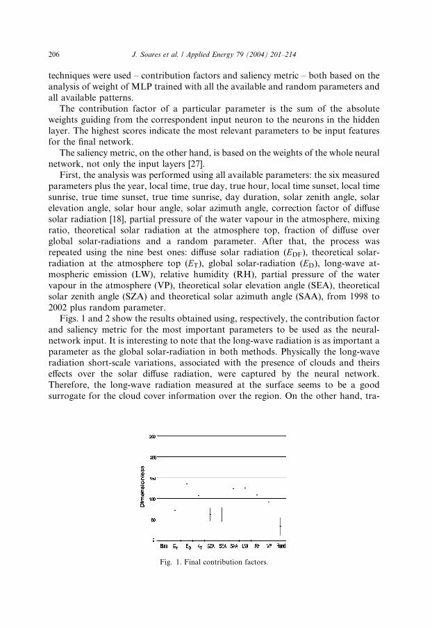
2002 plus random parameter.Figs. 1 and 2 show the results obtained using, respectively, the contribution factor

and saliency metric for the most important parameters to be used as the neural-

network input. It is interesting to note that the long-wave radiation is as important a

parameter as the global solar-radiation in both methods. Physically the long-wave

radiation short-scale variations, associated with the presence of clouds and theirs

effects over the solar diffuse radiation, were captured by the neural network.

Therefore, the long-wave radiation measured at the surface seems to be a good

surrogate for the cloud cover information over the region. On the other hand, tra-

Fig. 1. Final contribution factors.

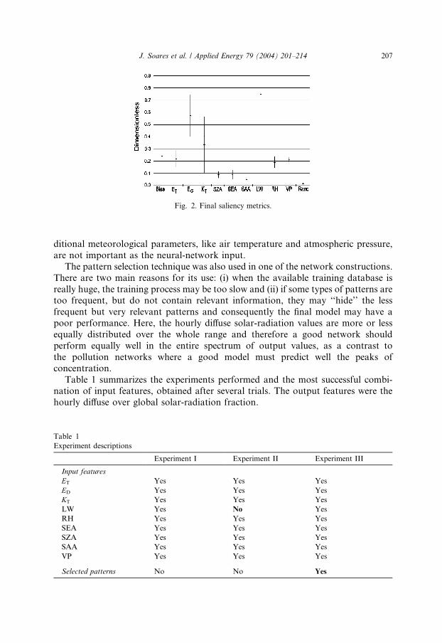
Fig. 2. Final saliency metrics.


ditional meteorological parameters, like air temperature and atmospheric pressure,

are not important as the neural-network input.

The pattern selection technique was also used in one of the network constructions.

There are two main reasons for its use: (i) when the available training database is

really huge, the training process may be too slow and (ii) if some types of patterns aretoo frequent, but do not contain relevant information, they may ‘‘hide’’ the less

frequent but very relevant patterns and consequently the final model may have a

poor performance. Here, the hourly diffuse solar-radiation values are more or less

equally distributed over the whole range and therefore a good network should

perform equally well in the entire spectrum of output values, as a contrast to

the pollution networks where a good model must predict well the peaks of

concentration.

Table 1 summarizes the experiments performed and the most successful combi-nation of input features, obtained after several trials. The output features were the

hourly diffuse over global solar-radiation fraction.

Table 1

Experiment descriptions

Experiment I Experiment II Experiment III

Input features

ET Yes Yes Yes

ED Yes Yes Yes

KT Yes Yes Yes

LW Yes No Yes

RH Yes Yes Yes

SEA Yes Yes Yes

SZA Yes Yes Yes

SAA Yes Yes Yes

VP Yes Yes Yes

Selected patterns No No Yes


5. Results

In all the experiments performed here, the standard back-propagation algorithm

was used with a learning rate of 0.5 and momentum of 0.9. Previous works show that

this selection of parameters leads to a quick and effective learning [26]. The networks

were trained using almost 4 years of data (January 1998fi September 2001) andverified using 1-year of data (2002) that was not presented during the network

training-period.

The first network (Experiment I) was trained with all available input features. To

verify the importance of the long-wave radiation as an input feature, Experiment II

was performed using as input all the input features used in Experiment I except for

long-wave radiation.

To try to improve the network performance, the final experiment (Experiment III)

was similar to Experiment I but included a pattern-selection technique. The idea wasto develop the reconstruction of the patterns with high values of diffuse solar-radi-

ation. Therefore, the neural network was trained with a higher percentage of patterns

having diffuse solar-radiation greater than unity. For that reason, it was used only

40% randomly of the patterns with diffuse solar-radiation less than unity and all

patterns with higher values of solar radiation.

5.1. Performance evaluation

To evaluate the performance of the MLP neural-networks, for the City of S~aoPaulo, a statistical comparison is performed using the indicator proposed by Stone

[16], a t-statistic (tS). This indicator is used along with two other well-known pa-

rameters: MBE and RMSE. Both MBE and RMSE have been specially employed as

adjustments of the solar-radiation models [3,11,28–30]. The RMSE and the MBE are

defined as follows:

MBE ¼XNi¼1

di=N

!;

and

RMSE ¼

ffiffiffiffiffiffiffiffiffiffiffiffiffiffiffiffiffiffiffiffiffiffiffiXNi¼1

dið Þ2=N2

vuut0@

1A:

Here, N is the total number of observations and di is the deviation between the ithcalculated value and the ith measured value.

The test of the MBE provides information on long-term performance of models

studied and, in general, a small MBE is desirable. The test on RMSE provides in-formation on the short-term performance of the models, as it allows a term-by-term

comparison of the actual deviation between the calculated value and the measured

value [28]. However, it is possible to have a large value for the RMSE and, simul-

taneously, a small value for the MBE, and vice versa.


Therefore, Stone [16] introduces the t-statistic as a new indicator of adjustment

between the calculated and measured data, defined as:

Table

Model

Cor

ob

ML

–

ML

–

ML

–

tc i

tS ¼ffiffiffiffiffiffiffiffiffiffiffiffiffiffiffiffiffiffiffiffiffiffiffiffiffiffiffiffiffiffiffiffiffiffiffiffiffiffiffiffiffiffiffiffiffiffiffiffiffiffiffiffiffiffiffiffiffiffiffiffiffiffiffiffiffiffiffiffiffiffiffiN � 1ð ÞMBE2= RMSE2 �MBE2

� �2

q� �:

To determine whether a model�s estimates are statistically significant, one has simply

to determine a critical tc value obtainable from standard statistical tables, e.g., tc(a=2) at the a level of significance, and N � 1 degrees of freedom [30].

A summary of the statistical parameters is shown in Table 2 for the values of EDF

obtained in Experiments I, I, III and using the correlation model obtained from [3].

The critical values are relative to a level of confidence of 95%. The worst statistical

result is given by the diffuse-radiation hourly values derived for S~ao Paulo using the

correlation model. The best result was obtained by Experiment III, but it still is not

inside the acceptance region. Once that the hourly values of solar radiation are very

sensitive to the cloud cover, the improvement obtained in Experiment I when

compared with Experiment II (without long-wave radiation) seems to confirm that

the long-wave radiation can be used as a surrogate for the cloud cover over theregion.

5.2. Comparison between MLP and correlation model

Hereafter, due to the best statistic performance of Experiment III, the discussion

will be focused only on this experiment.

The dispersion diagrams between the hourly values of diffuse solar-radiation

observed and obtained using MLP network are displayed in Fig. 3. The coefficientcorrelation obtained using MLP (Fig. 3(a); r ¼ 0:94) is larger than that using the

correlation model (Fig. 3(b); r ¼ 0:91), so indicating the better performance of the

MLP network.

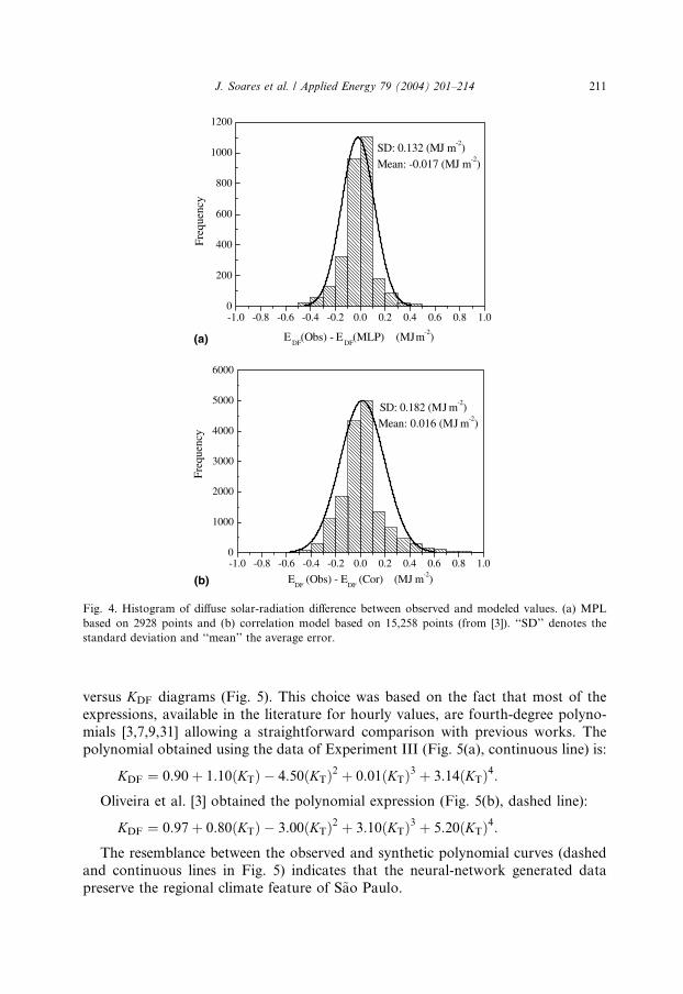
Histograms of the differences between the solar diffuse-radiation synthetic and

observed are shown in Fig. 4. The standard deviation and the mean-error value are

also presented in the figure. In the case of MLP and of the correlation model, the

2

statistics

Sample size (h) MBE (MJm�2) RMSE (MJm�2) tS tc

relation model

tained from [3]

15258 )0.0169 0.193 11.16 1.96

P neural-network

Experiment I

2928 0.0116 0.121 5.19 1.96

P neural-network

Experiment II

2928 0.0291 0.152 10.63 1.96

P neural-network

Experiment III

2928 0.0110 0.155 3.86 1.96

s given at a level of confidence of 95%.

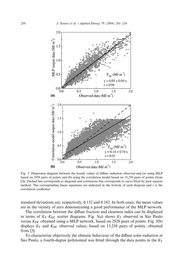
Fig. 3. Dispersion diagram between the hourly values of diffuse radiation observed and (a) using MLP

based on 2928 pairs of points and (b) using the correlation model based on 15,258 pairs of points (from

[3]). Dashed line corresponds to diagonal and continuous line corresponds to curve fitted by least squares

method. The corresponding linear equations are indicated in the bottom of each diagram and r is the

correlation coefficient.


standard deviations are, respectively, 0.132 and 0.182. In both cases, the mean values

are in the vicinity of zero demonstrating a good performance of the MLP network.

The correlation between the diffuse fraction and clearness index can be displayed

in terms of KT–KDF scatter diagrams. Fig. 5(a) shows KT observed in S~ao Paulo

versus KDF obtained using a MLP network, based on 2928 pairs of points. Fig. 5(b)

displays KT and KDF observed values, based on 15,258 pairs of points, obtained

from [3].To characterize objectively the climatic behaviour of the diffuse solar-radiation at

S~ao Paulo, a fourth-degree polynomial was fitted through the data points in the KT

-1.0 -0.8 -0.6 -0.4 -0.2 0.0 0.2 0.4 0.6 0.8 1.00

200

400

600

800

1000

1200

SD: 0.132 (MJ m-2)Mean: -0.017 (MJ m-2)

(a)

Freq

uenc

y

EDF

(Obs) - EDF

(MLP) (MJm-2)

-1.0 -0.8 -0.6 -0.4 -0.2 0.0 0.2 0.4 0.6 0.8 1.00

1000

2000

3000

4000

5000

6000

SD: 0.182 (MJ m-2)Mean: 0.016 (MJ m-2)

(b)

Freq

uenc

y

EDF

(Obs) - EDF

(Cor) (MJ m-2)

Fig. 4. Histogram of diffuse solar-radiation difference between observed and modeled values. (a) MPL

based on 2928 points and (b) correlation model based on 15,258 points (from [3]). ‘‘SD’’ denotes the

standard deviation and ‘‘mean’’ the average error.


versus KDF diagrams (Fig. 5). This choice was based on the fact that most of the

expressions, available in the literature for hourly values, are fourth-degree polyno-

mials [3,7,9,31] allowing a straightforward comparison with previous works. Thepolynomial obtained using the data of Experiment III (Fig. 5(a), continuous line) is:

KDF ¼ 0:90þ 1:10 KTð Þ � 4:50 KTð Þ2 þ 0:01 KTð Þ3 þ 3:14 KTð Þ4:
Oliveira et al. [3] obtained the polynomial expression (Fig. 5(b), dashed line):
KDF ¼ 0:97þ 0:80 KTð Þ � 3:00 KTð Þ2 þ 3:10 KTð Þ3 þ 5:20 KTð Þ4:
The resemblance between the observed and synthetic polynomial curves (dashed
and continuous lines in Fig. 5) indicates that the neural-network generated data

preserve the regional climate feature of S~ao Paulo.

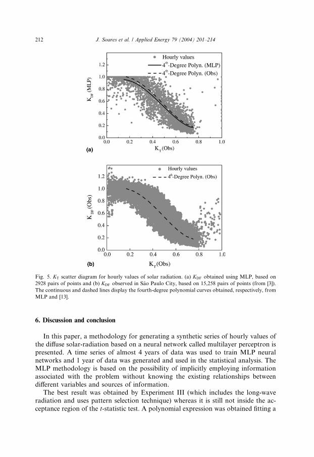
Fig. 5. KT scatter diagram for hourly values of solar radiation. (a) KDF obtained using MLP, based on

2928 pairs of points and (b) KDF observed in S~ao Paulo City, based on 15,258 pairs of points (from [3]).

The continuous and dashed lines display the fourth-degree polynomial curves obtained, respectively, from

MLP and [13].


6. Discussion and conclusion

In this paper, a methodology for generating a synthetic series of hourly values of

the diffuse solar-radiation based on a neural network called multilayer perceptron is

presented. A time series of almost 4 years of data was used to train MLP neural

networks and 1 year of data was generated and used in the statistical analysis. TheMLP methodology is based on the possibility of implicitly employing information

associated with the problem without knowing the existing relationships between

different variables and sources of information.

The best result was obtained by Experiment III (which includes the long-wave

radiation and uses pattern selection technique) whereas it is still not inside the ac-

ceptance region of the t-statistic test. A polynomial expression was obtained fitting a


fourth-degree polynomial through the data points of KT observed for S~ao Paulo

versus KDF obtained using the MLP network. The resemblance between the observed

and synthetic curves indicates that the neural-network generated data preserve the

feature of the regional climate of S~ao Paulo.

A significant result is the importance of atmospheric long-wave radiation as a

surrogate for the cloud-cover information on the regional scale, a very difficult pa-rameter to measure and express in diffuse solar-radiation models. By contrast, tra-

ditional meteorological parameters, like air temperature and atmospheric pressure,

are not as important as long-wave radiation.

Acknowledgements

This research was sponsored by CNPq (Conselho Nacional de Desenvolvimento

Cient�ıfico e Tecnol�ogico) during the collaboration program Brazil-Slovenia (Proc.

CNPq No. 490017/02-9). On the Slovenian side, the research was sponsored by theAMES company and the Slovenian Ministry for school, science and sport during the

same colaboration program.

References

[1] Collares-Pereira M, Rabl A. The average distribution of solar radiation – correlation between diffuse

and hemispherical and between daily and hourly insolation values. Solar Energy 1979;22:155–64.

[2] Gonz�alez J-A, Calb�o J. Influence of the global radiation variability on the hourly diffuse fraction

correlations. Solar Energy 1999;65(2):119–31.

[3] Oliveira AP, Escobedo JF, Machado AJ, Soares J. Correlation models of diffuse solar-radiation

applied to the City of S~ao Paulo (Brazil). Appl Energy 2002;71(1):59–73.

[4] Iqbal M. An introduction to solar radiation. Academic Press; 1983. 390 pp.

[5] Liu BYH, Jordan RC. The interrelationship and characteristic distribution of direct, diffuse and total

solar radiations. Solar Energy 1960;4:1–9.

[6] Collares-Pereira M, Rabl A. The average distribution of solar radiation – correlation between diffuse

and hemispherical and between daily and hourly insolation values. Solar Energy 1979;22:155–64.

[7] Erbs DG, Klein SA, Duffie JA. Estimation of the diffuse-radiation fraction for hourly, daily and

monthly-average global radiations. Solar Energy 1982;28:293–302.

[8] Satyamurti VV, Lahiri PK. Estimation of symmetric and asymmetric hourly global and diffuse

radiations from daily values. Solar Energy 1992;48:7–14.

[9] Jacovides CP, Hadjioannou L, Passhiardis S, Stefanou L. On the diffuse fraction of daily and monthly

global radiation for the Island of Cyprus. Solar Energy 1996;56:565–72.

[10] LeBaron B, Dirmhirn I. Strengths and limitations of the Liu and Jordan model to determine diffuse

from global irradiance. Solar Energy 1983;31:167–72.

[11] Soler A. Dependence on latitude of the relation between the diffuse fraction of solar radiation and the

ratio of global-to-extraterrestrial radiation for monthly average daily values. Solar Energy

1990;44:297–302.

[12] Rumelhart DE, Hilton GE, Williams RJ. Learning internal representation by error propagation. In:

Rumelhart DE, McClelland JL, editors. Parallel distributed processing: explorations in the

microstructure of cognition, vol. 1. Cambridge, MA: MIT Press; 1986.

[13] Lawrence J. Data preparation for a neural network. Artif Intell Expert 1991:34–41.

[14] Sfetsos A, Coonick AH. Univariate and multivariate forecasting of hourly solar-radiation with

artificial-intelligence techniques. Solar Energy 2000;68(2):169–78.


[15] L�opez G, Rubio MA, Martinez M, Batlles FJ. Estimation of hourly global photosynthetically-active

radiation using artificial neural-network models. Agri Forest Meteorol 2001;107:279–91.

[16] Stone RJ. Improved statistical procedure for the evaluation of solar-radiation estimation models.

Solar Energy 1993;51:289–91.

[17] Oliveira AP, Escobedo JF, Machado AJ, Soares J. Diurnal evolution of solar radiation at the surface

in the City of S~ao Paulo: seasonal variation and modeling. Theoret Appl Climatol 2002;71(3-4):231–

49.

[18] Oliveira AP, Escobedo JF, Machado AJ. A new shadow-ring device for measuring diffuse solar

radiation at the surface. J Atmos Oceanic Technol 2002;19(5):698–708.

[19] Dana G. Procedures for correcting Eppley pyrgeometer data; 1996. Available from http://

huey.colorado. edu/LTER/datasets/meteorology/pyrgeometer.html.

[20] Fairall CW, Persson POG, Bradley EF, Payne RE, Anderson SP. A new look at calibration and use of

Eppley precision infrared radiometers. Part I: Theory and application. J Atmos Oceanic Technol

1998;15:1229–42.

[21] Reda I, Hickey JR, Stoffel T, Myers D. Pyrgeometer calibration at the National Renewable Energy

Laboratory (NREL). J Atmos Solar-Terrestrial Phys 2002;64:1623–9.

[22] Schalkoff R. Pattern recognition: statistical structural and neural approaches. New York: Wiley; 1992.

[23] Hornik K. Approximation capabilities of multilayer feedforward networks. Neural Networks

1991;4:251–7.

[24] Gardner MW, Dorling SR. Artificial neural-networks (the multilayer perceptron) – a review of

applications in the atmospheric Sciences. Atmos Environ 1998;32:2627–36.

[25] Bonar M, Mlakar P. Improvement of air-pollution forecasting models using feature determination

and pattern selection strategies. In: Gryning S-E, Chaumerliac N, editors. Air-pollution modeling and

its application XII (NATO challenges of modern society). New York, London: Plenum Press; 1998. p.

725–26.

[26] Mlakar P, Bonar M. Perceptron neural-network-based model predicts air pollution. In: Adeli H,

editor. Intelligent Information Systems IIS�97, Grand Bahama Island, Bahamas, December 8–10,

1997. Proceedings. Los Alamos, CA: IEEE Computer Society; 1997. p. 345.

[27] Mlakar P. Determination of features for air-pollution forecasting models. In: Adeli H, editor.

Intelligent Information Systems IIS�97, Grand Bahama Island, Bahamas, December 8–10, 1997.

Proceedings. Los Alamos, CA: IEEE Computer Society; 1997. p. 350–54.

[28] Halouani N, Ngguyen CT, Vo-Ngoc D. Calculation of monthly average global solar radiation on

horizontal surfaces using daily hours of bright sunshine. Solar Energy 1993;50(3):247–58.

[29] Ma CCY, Iqbal M. Statistical comparison of solar radiation correlations. Monthly average global and

diffuse radiation on horizontal surfaces. Solar Energy 1984;33(2):143–8.

[30] Targino ACL, Soares J. Modeling surface energy-fluxes for Iper�o, SP, Brazil: an approach using

numerical inversion. Atmos Res 2002;63(1):101–21.

[31] Newland FJ. A study of solar-radiation modes for the coastal region of South China. Solar Energy

1989;43:227–35.

http://huey.colorado.edu/LTER/datasets/meteorology/pyrgeometer.html

http://huey.colorado.edu/LTER/datasets/meteorology/pyrgeometer.html

Documents

Modeling hourly diffuse solar-radiation in the city of São Paulo using a neural-network technique