Modeling for Insight Using Tools for Energy Model Optimization andAnalysis (Temoa)

Kevin Huntera,∗, Sarat Sreepathib, Joseph F. DeCarolisa

North Carolina State University, Raleigh, NC 27695, USA

aDepartment of Civil, Construction, and Environmental EngineeringbDepartment of Computer Science

Abstract

This paper introduces Tools for Energy Model Optimization and Analysis (Temoa), an open sourceframework for conducting energy system analysis. The core component of Temoa is an energy economyoptimization (EEO) model, which minimizes the system-wide cost of energy supply by optimizing thedeployment and utilization of energy technologies over a user-specified time horizon. The design of Temoa isintended to fill a unique niche within the energy modeling landscape by addressing two critical shortcomingsassociated with existing models: an inability to perform third party verification of published model resultsand the difficulty of conducting uncertainty analysis with large, complex models. Temoa leverages a modernrevision control system to publicly archive model source code and data, which ensures repeatability of allpublished modeling work. From its initial conceptualization, Temoa was also designed for operation within ahigh performance computing environment to enable rigorous uncertainty analysis. We present the algebraicformulation of Temoa and conduct a verification exercise by implementing a simple test system in both Temoaand MARKAL, a widely used commercial model of the same type. In addition, a stochastic optimizationof the test system is presented as a proof-of-concept application of uncertainty analysis using the Temoaframework.

Keywords: energy economy, open source, repeatability, uncertainty analysis, stochastic optimization

1. Introduction

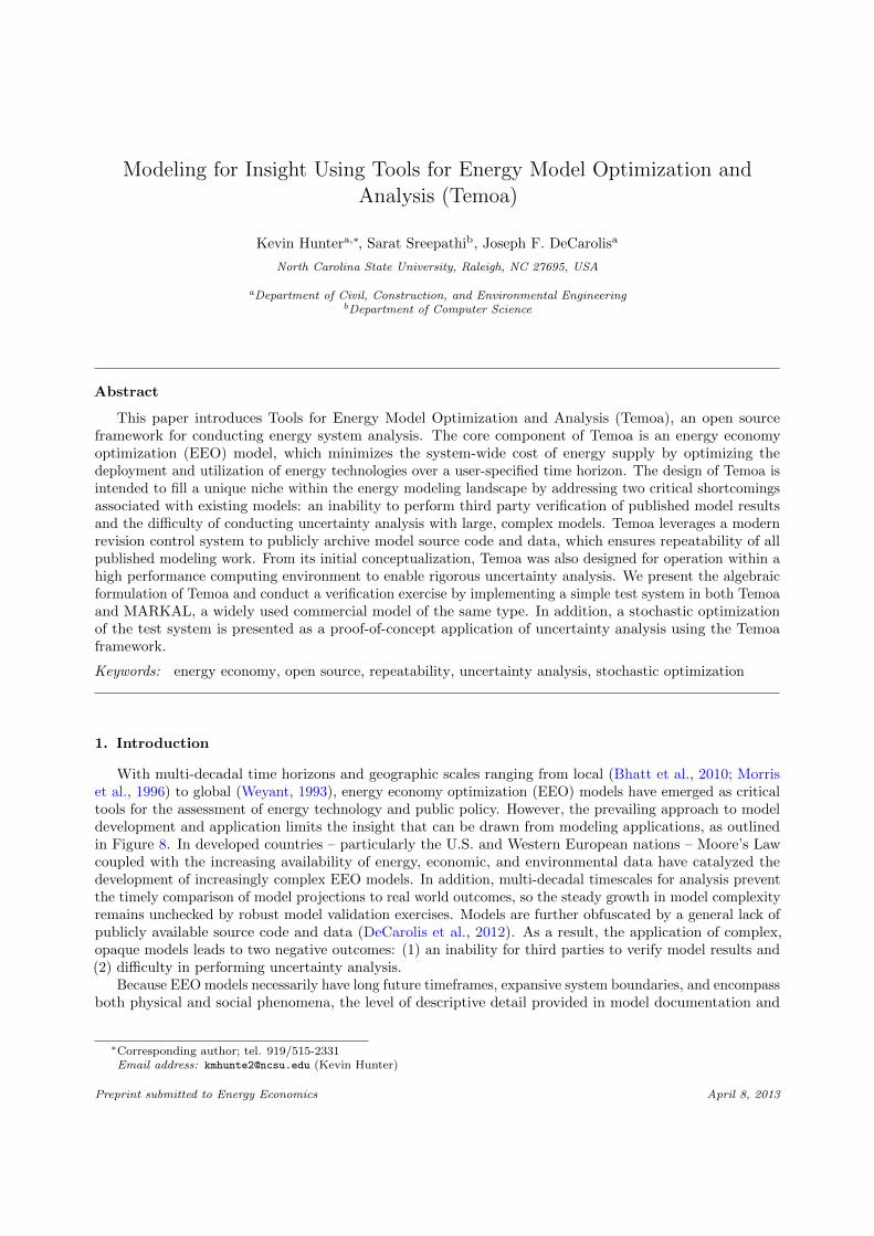
With multi-decadal time horizons and geographic scales ranging from local (Bhatt et al., 2010; Morriset al., 1996) to global (Weyant, 1993), energy economy optimization (EEO) models have emerged as criticaltools for the assessment of energy technology and public policy. However, the prevailing approach to modeldevelopment and application limits the insight that can be drawn from modeling applications, as outlinedin Figure 8. In developed countries – particularly the U.S. and Western European nations – Moore’s Lawcoupled with the increasing availability of energy, economic, and environmental data have catalyzed thedevelopment of increasingly complex EEO models. In addition, multi-decadal timescales for analysis preventthe timely comparison of model projections to real world outcomes, so the steady growth in model complexityremains unchecked by robust model validation exercises. Models are further obfuscated by a general lack ofpublicly available source code and data (DeCarolis et al., 2012). As a result, the application of complex,opaque models leads to two negative outcomes: (1) an inability for third parties to verify model results and(2) difficulty in performing uncertainty analysis.

Because EEO models necessarily have long future timeframes, expansive system boundaries, and encompassboth physical and social phenomena, the level of descriptive detail provided in model documentation and

∗Corresponding author; tel. 919/515-2331Email address: kmhunte2@ncsu.edu (Kevin Hunter)

Preprint submitted to Energy Economics April 8, 2013

K. Hunter et al., 2013

peer-reviewed journals is insufficient to reproduce a specific set of published results. More generally, theprecise replication of results with computational models requires access to source code and data (Ince et al.,2012; Hanson et al., 2011; Barnes, 2010).

Large, complex models are also computationally expensive and therefore difficult to iterate, which detersefforts to perform sensitivity and uncertainty analysis. As a result, treatment of uncertainty in EEO model-based analysis is often limited (e.g., EIA, 2012; Clarke et al., 2007; Nakicenovic et al., 2000; IEA, 2010).Complex models are often used to produce a small number of illustrative scenarios that contribute relativelylittle insight about the system under consideration (Morgan and Henrion, 1990). The focus on a limitedset of highly detailed scenarios can also produce cognitively compelling storylines that lead to systematicoverconfidence in the results presented (Morgan and Keith, 2008). The poor performance associated withpast efforts to predict future energy outcomes supports this assertion (Craig et al., 2002).

This paper introduces Tools for Energy Model Optimization and Analysis (Temoa), an open sourcemodeling framework used to conduct energy system analysis with a technology explicit energy economyoptimization (EEO) model. We aim to address the issues of verification and uncertainty quantification by (1)instituting a transparent process for EEO model development and application that facilitates independentthird party verification, and (2) implementing rigorous uncertainty analysis in a high performance computing(HPC) environment. Section 2 outlines our long term goals and justification for creating Temoa. Section 3describes how Temoa will meet our stated objectives. Section 4 gives an overview of the model’s algebraicformulation, and Section 5 describes the software used to implement the Temoa formulation. Section 6presents a verification exercise based on careful comparison to a simple MARKAL dataset. Section 7 presentsa proof-of-concept application of stochastic optimization to illustrate the capability of the Temoa frameworkto conduct uncertainty analysis, and Section 8 draws conclusions and outlines future work.

2. Motivation

Energy model design should be driven by a clearly articulated research goal. Our long-term goal isto derive policy-relevant insight related to the cost, emissions, deployment, and coordinated operation ofenergy technologies over time while rigorously accounting for large future uncertainties. While simple andtransparent accounting frameworks can be utilized to conduct such analysis, the specification of detailed,self-consistent assumptions across the energy system can be difficult and time consuming. By contrast,optimization models employ formal search techniques, which enable a rapid and systematic exploration ofthe decision space to identify solutions that meet a specified objective. We chose to build a technologyexplicit EEO model, which enables a simultaneously broad and deep assessment of technology by consideringthe economic and technical characteristics of individual technologies as well as their interactions within awell-defined system.

Prior to building Temoa, we conducted an extensive review of existing energy models (DeCarolis et al.,2012). Through a formal review of the International Energy Workshop annals over the last decade, wefound that three-fourths of surveyed models do not provide access to model source code and data. Amongthose that do, OSeMOSYS (Howells et al., 2011) is closest in structure and function to Temoa but serves acomplementary purpose. A key motivation for OSeMOSYS is to make energy system modeling accessible toa much broader community, including students and researchers in developing countries who often lack thetime and financial resources required to utilize larger commercial models. While the Temoa project sharesthese goals by utilizing free software, its design was driven primarily by the desire to enable repeatability andperform uncertainty analysis. We believe that there is value in having more than one open source EEO modelof the same type available to the energy modeling community, since two distinct models are never identical:the process of distilling the relevant literature into a mathematical model requires reasoned judgment thatmakes modeling as much art as science (Morrison and Morgan, 1999; Ravetz, 2003).

In addition to reviewing the process of EEO model development and application, DeCarolis et al. (2012)also investigated the broader field of scientific computing and used it to develop a set of recommendationsthat can help enable the replication of model-based results by third parties. The recommendations includemaking source code and input data publicly accessible, making transparency a design goal, and utilizing freesoftware tools. We have implemented these recommendations in the design of the Temoa framework.

2

K. Hunter et al., 2013

3. The Temoa Framework

The Temoa framework is designed such that the resultant model-based analysis is repeatable by thirdparties and provides an assessment of uncertainty that can affect outcomes of interest. We describe inSection 3.1 – Section 3.3 how these design objectives were met.

3.1. Transparency

To inform our approach to model transparency, we investigated the software engineering practicesemployed by three large scale scientific software projects: MPICH2, a high performance parallel programminglibrary (Balaji et al., 2011); the Portable, Extensible Toolkit for Scientific Computation (PETSc), a paralleldifferential equations solver library (Balay et al., 2011); and the Community Earth System Model (CESM), afully-coupled, global climate model (UCAR, 2013). Based on careful review of these projects, the Temoaframework has been designed to include the following features: (1) a public, web-enabled interface to modelsource code and data, (2) developer documentation to encourage community contributions, (3) an avenue foruser and developer interaction, and (4) a software utility to visualize output.

3.1.1. Revision Control

The Temoa project provides public, web-enabled access to a revision control system (RCS), which providesthe means to digitally store a complete archive of code changes (i.e., “commit” or “change” histories). Bestpractices suggest that the developer summarizes each commit to the repository. The resultant electronicarchive enables structured development and provides an audit trail that enhances transparency for bothTemoa developers and users.

A project may organize an RCS in a number of ways. One common approach divides the repository into atrunk and development branches, with the trunk representing the latest version, and the individual branchesrepresenting stable versions or experiments. Temoa’s repository structure includes parallel developmentbranches (and no trunk) with each branch tuned to explore a specific set of questions. In many cases, whereadditional functionality requires extensive modification to an existing model formulation, the existing versioncan remain distinct and be archived separately. By archiving different branches of Temoa, we intend toprevent creep in model complexity over time as a model is adapted to answer new questions. Our approachcontrasts with OSeMOSYS, which is based on the development of separable component blocks that can beadded or removed to a core version of the model to customize model functionality (Howells et al., 2011). Bothapproaches have strengths, but neither is perfect: it may be difficult to separate OSeMOSYS functionalityinto distinct component blocks, but it may also be difficult to integrate changes across different versions andbranches of Temoa.

3.1.2. Documentation

While public access to code and data enables interested parties to interrogate the model, it will remainlargely opaque in the absence of well-designed user documentation. We have implemented auto-generateddocumentation that fuses comment blocks in the source code with a clear narrative description. As describedin Section 5, the Temoa model has been implemented in Python (Lutz, 2009). Python stores object commentsin a special member variable, allowing third party tools to dynamically introspect a code base to generatedocumentation accessible to end users. In Temoa, comments interspersed in the source code contain LaTeX(Lamport, 1986) formatted algebraic formulations of associated equations that are automatically queried andcombined with a separate descriptive narrative to dynamically create end-user documentation. The latestdocumentation is available on the project website (Hunter et al., 2013). This streamlines the documentationeffort by allowing developers to focus on embedding descriptive comments in the source code, which alsoeliminates discrepancies that arise from maintaining multiple forms of documentation.

3.1.3. Communication and Interaction

A successful open source model must provide a means for users and developers to interact. The developersof PETSc and MPICH2 are highly responsive to user queries on their traffic-intensive mailing lists (MPICH2,2013; PETSc, 2012). While currently we do not have the same traffic as these well-established projects, weuse an online forum for communication among developers as well as interaction with end users.

3

K. Hunter et al., 2013 3.2 Replication of Model Results

3.1.4. Visualization

Both PETSc and CESM include visualization tools to help users interrogate model behavior. In our case,model accessibility and transparency relies in part on the capability to visualize the energy system networkunder consideration. To meet this need, we employ an open source graphics package called Graphviz (Ellsonet al., 2002) to dynamically generate an energy system map at model runtime. The Graphviz layout programstake descriptions of graphs in a simple text language, and create diagrams in several formats. Graphvizoperates on a text file produced at model runtime that describes the nodes and edges within a given graph.Figure 8 provides an illustrative energy system map. Temoa also generates a set of navigable output graphicsby model time period that superimpose the resultant commodity flows and technology capacities on thegraph. In addition to the output graphic, the Graphviz text input provides an auditable model record thatcan be used for debugging and verification purposes.

3.2. Replication of Model Results

The RCS serves another important objective: to archive “snapshots” of source code and data used toproduce published model analysis. To our knowledge, Temoa is the first EEO modeling effort to providepublic access to a revision control system, which enables third parties to precisely replicate our publishedresults by accessing archived versions of source code and data. While other open source models such asOSeMOSYS (Howells et al., 2011), AIM (Kainuma et al., 1998), and DICE (Nordhaus, 1993) exist, nonepublicly archive source code and data in a consistent manner that enables precise replication of publishedresults by third parties.

3.3. Uncertainty Analysis

A key challenge associated with energy modeling is to derive actionable insight in the face of large futureuncertainties. Many prior efforts have made future uncertainty the focus of model-based analysis (Kanudiaand Loulou, 1998; Gritsevskyi and Nakicenovi, 2000; Labriet et al., 2008). From its initial conceptualization,Temoa was designed for operation in a multi-core, multi-node compute environment, which significantlyexpands the capability to perform sensitivity and uncertainty analysis. We do not intend to use the enhancedcomputational ability to solve large and complex datasets. Rather, our intention is to build datasets that areonly as detailed as needed to meet the research objective at hand, and to focus effort on iterating the modelto understand how key uncertainties can drive the model results.

Model uncertainties can arise from two sources: the imprecise specification of input data (parametricuncertainty) and the limited ability of model equations to represent reality (structural uncertainty). Parametricuncertainty can be addressed in a variety of ways: scenario analysis to quantify how exogenous drivers affectmodel outputs, sensitivity analysis to identify the input parameters that produce the largest effect on modeloutputs, and uncertainty analysis via Monte Carlo simulation to provide a measure of dispersion in theoutputs. Running an energy model in an HPC environment facilitates sensitivity and uncertainty analysis byenabling the simultaneous execution of multiple model runs across available compute cores.

Because each model realization produced with one of the techniques above assumes (a priori) a particularstate of the world based on the input values drawn, the parameter uncertainty is propagated throughthe model. Resolution of uncertainty before the optimization is performed represents a “learn then act”approach (Kann and Weyant, 2000). Such an approach is of limited utility to a decision maker, who mustmake decisions in the face of uncertainty by taking an “act then learn” approach. Multi-stage stochasticoptimization embeds the probability of different outcomes within the model formulation via specificationof an event tree, yielding a near term hedging strategy that accounts for future uncertainties (Loulou andLehtila, 2007). Such hedging strategies provide insight relevant to policy makers, investors, and planners,who must make decisions before uncertainty is resolved (Holthausen, 1979). The complexity of event treesis often limited by the computational difficulty in solving the extensive form of the problem specificationwith classical solution methods. While stochastic optimization has been applied to energy system models,the model complexity and computational requirements have limited analysis to relatively simple probabilitytrees. For example, Kanudia and Loulou (1998) implemented 8 scenarios across 3 time stages, Loulou andKanudia (1999) implemented 5 scenarios across 2 time stages, Labriet et al. (2008) implemented 8 scenarios

4

K. Hunter et al., 2013

across 2 time stages, Bosetti and Tavoni (2009) implemented 3 scenarios across two stages, and Babonneauet al. (2012) implemented 4 scenarios across 2 time stages. The implementation of the Temoa framework ona compute cluster using solution algorithms that involve the use of distributed memory, such as progressivehedging (Watson and Woodruff, 2010), allow the specification of event trees that are more complex, therebyenabling us to address future uncertainty in a more comprehensive manner. Section 7 discusses a stochasticoptimization of a simple model with 81 scenarios across 3 time stages, and we have solved internal testformulations with 512 scenarios across 4 time stages (albeit with a simple energy system representation).

All of the techniques discussed thus far address parametric uncertainty. Given the limited ability of EEOmodels to represent real world energy markets, structural uncertainty is a critical consideration. In futurework, we plan to address the structural uncertainty in the Temoa model formulation through the applicationof modeling-to-generate alternatives, which provides a way to systematically search the model’s near optimaldecision space for alternative solutions that account for unmodeled objectives (DeCarolis, 2011).

4. Model Formulation

The core component of the Temoa framework is a technology explicit energy system model. The modelobjective is to minimize the present cost of energy supply by deploying and utilizing energy processes andcommodities over time to meet a set of exogenously specified end-use demands. The energy system isdescribed algebraically as a network of linked processes that convert raw energy commodities (e.g., coal, oil,biomass, uranium, sunlight) into end-use demands (e.g., lighting, transport, water heating) through a seriesof one or more intermediate energy forms (e.g., electricity, gasoline, ethanol). Each process is defined by aset of engineering, economic, and environmental characteristics (e.g., capital cost, efficiency, capacity factor,emissions rate) associated with converting an energy commodity from one form to another. Processes arelinked together in a network via model constraints representing the allowable flow of energy commodities.

Technology explicit models are typically formulated as linear programming problems in which continuousamounts of technology capacity are utilized to meet end-use demands. In cases where non-linear relationshipsexist, such as supply curves for raw energy commodities, a piecewise linear approach can be taken (Loulouet al., 2004). The Temoa model formulation is similar to the MARKAL/TIMES model generators (Fishboneand Abilock, 1981; Loulou et al., 2005), MESSAGE (Messner and Strubegger, 1995), and OSeMOSYS(Howells et al., 2011).

4.1. Treatment of Time

The Temoa model optimizes energy system infrastructure and performance across several timescales.The longest scale is the complete set of periods (P ) considered by the model, which is in turn divided intotwo distinct sets: ‘existing’ (P e), and ‘future’ (P f ). The existing time set defines the technology capacityvintages that exist prior to the periods in the future time set, and the model will return results for theperiods in the future time set.

Both time sets (P e and P f ) consist of user-defined periods, which represent an aggregation of the yearsfrom one period to the next. For example, if the first three time periods in a Temoa model are 2010, 2015,and 2025, then the 2010 time period represents the years 2010 through 2014, and the 2015 time periodrepresents the years 2015 through 2024. Note that the length of each period is determined dynamically fromthe time between adjacent periods in P f , allowing (for example) the user to specify shorter periods near thepresent and longer periods into the future when uncertainty is larger. Within each period, Temoa performsthe optimization for a single characteristic year, with all capacity and activity results assumed to remainthe same for every year within the period. As such, the optimal results for each period correspond to arepresentative year within that period.

To capture the seasonal and diurnal variations in end-use demand and required technology capacity, eachfuture year is divided into sets of seasons and times of day. Combinations of each season and time of dayform time slices (e.g., winter-day, summer-night). The formulation in Sections 4.2 - 4.6 describes how Temoaoptimizes technology capacity and utilization across these time units.

5

K. Hunter et al., 2013 4.2 Introduction to Model Algebra

4.2. Introduction to Model Algebra

Algebraic models generally consist of four distinct components: sets, parameters, variables, and equations.A set is a collection of user-specified elements used by the model to index parameters and variables. Forexample, Temoa contains a set T that represents the set of all technologies considered by the model. Theuser must define the elements of T (e.g., pulverized coal, wind, electric car), which Temoa uses to indexvarious parameters and variables. For instance, the investment cost ICt,v is indexed by t ∈ T and v ∈ Vsuch that each defined vintage of each technology is assigned an investment cost.

Table 1 explains the nomenclature in Temoa’s formulation. There are a total of 6 unique sets as well asseveral subsets and alias sets. Capital subscripts represent the set names and lower case subscripts representindividual set elements (e.g., c ∈ C). Note that all commodities (c) belong to the set C, but for notationalclarity in the formulation, we define aliases for individual set elements to represent input commodities(i ∈ C) and output commodities (o ∈ C). Note also that because most parameters, variables, and constraintsare sparsely indexed, Θ denotes the sparse superset representing the valid combinations of individual setelements. The subscript to Θ denotes a specific sparse superset, which can be identified by context. Forexample, the Demand constraint class (eq. 3) is only useful for the specific indices of the end-use demand anddemand-specific distribution parameters (p, s, d, and c) that are specified by the modeler in the associateddata file. We denote this sparse subset of valid indices by Θdemand.

The ordering of the set indices is consistent throughout the model to promote an intuitive “left-to-right”description of each parameter, variable, and constraint set. For example, Temoa’s output commodity flowvariable FOp,s,d,i,t,v,o can be described as follows: “in period (p) during season (s) at time of day (d), theflow of input commodity (i) to technology (t) of vintage (v) generates an output commodity flow (o) ofFO.” While not all variables and parameters are indexed by all the sets shown above, they all follow thesame left-to-right ordering scheme. In this manner, for any indexed parameter or variable within Temoa, aleft-to-right, arrow-box-arrow describes the input→process→output flow of energy. A visual depiction of thecommodity flow into and out of a given process is provided in Figure 8.

A key parameter is technology efficiency EFF i,t,v,o, which defines the output (o) per unit input (i) ofeach process 〈t, v〉. Temoa uses the modeler-specified indices of the EFF parameter to build the sparse Θsuperset of valid indices for every other parameter, variable, and constraint.

4.3. Decision Variables

The lowest level decision variable in the model is the commodity flow out of a technology (FO). Thetechnology- and vintage-specific activity and capacity are in turn derived from FO. In Temoa, the totalcommodity production from a process is referred to as its “activity”:

Process Activity :

ACTp,s,d,t,v =∑i,o

FOp,s,d,i,t,v,o (1)

∀{p, s, d, t, v} ∈ Θactivity

Since the activity variable (ACT) is given by the sum over the commodity inputs and outputs associatedwith the output flow variable FO, a technology’s activity level is always measured by its commodity productionrather than consumption. The summation over both i and o is required to accommodate a many-to-oneor many-to-many input-output commodity mapping. The ACT variable in turn determines the requiredtechnology capacity (CAP):

6

K. Hunter et al., 2013 4.4 Physical and Operational Constraints

Technology Capacity :

(CF s,d,t,v · C2At · SEGs,d · TLF p,t,v) ·CAPt,v ≥ ACTp,s,d,t,v (2)

∀{p, s, d, t, v} ∈ Θactivity

The capacity factor (CF ) represents the maximum availability of a process by season and time-of-day, asdetermined by resource availability (e.g., as with intermittent renewables) as well as forced and unforcedoutage rates. The segment (SEG) is critical because the required amount of technology-specific capacitydepends on the period of time over which the production occurs. For processes whose lifetimes end withinperiod p, Equation (2) limits the activity by the scaling factor TLF . The user is responsible for ensuringthe consistency among units through the proper specification of C2A. While the CAP variable relates toACT via an inequality constraint, the constraint will remain binding where new capacity has a positivecost. Equation (2) also applies to preexisting capacity, where the variable CAP is replaced by the parameterECAP .

4.4. Physical and Operational Constraints

There are several constraints required to represent the critical physical and operational requirementsassociated with an energy system. The requirement that supply is sufficient to meet demand drives all otherconstraints: the model must ensure that the exogenously specified annual end-use demands (DEMp,c) –distributed per slice according to the demand-specific distribution (DSDs,d,c) – are satisfied by the availablecommodity output:

Supply-Demand Constraint : ∑i,t,v

FOp,s,d,i,t,v,c ≥ DEMp,c ·DSDs,d,c (3)

∀{p, s, d, c ∈ Cd} ∈ Θdemand

While Equation (3) requires commodity production to meet an end-use demand, it does not specify howthe end-use commodities are produced. A constraint is needed to determine how commodity inputs andoutputs relate at the individual process level:

Process-Level Commodity Flow Constraint :

FOp,s,d,i,t,v,o ≤ EFF i,t,v,o · FIp,s,d,i,t,v,o (4)

∀{p, s, d, i, t ∈ T − T s, v, o} ∈ Θflow

Equation (4) ensures that the commodity output of a process cannot exceed the product of the commodityinput and efficiency, enforcing conservation of energy at the process level. In addition, indexing efficiencyby both input and output commodities provides a flexible technology characterization capable of trackingmultiple commodity flows into and out of a single technology. For example, a flex fuel vehicle can consumean ethanol blend or gasoline to produce vehicle miles traveled, each with different efficiencies. (Note thatT − T s indicates the subset of T that does not include T s. Thus, Equation (4) applies to all non-storageprocesses.) Equations (3) and (4) ensure that demand is met by a demand technology, but an additionalconstraint is needed to connect the inputs to demand technologies with upstream outputs:

7

K. Hunter et al., 2013 4.4 Physical and Operational Constraints

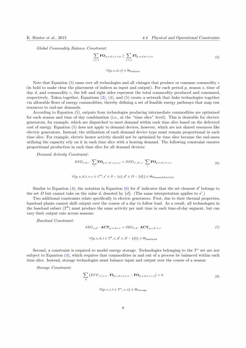
Global Commodity Balance Constraint :∑i,t,v

FOp,s,d,i,t,v,c ≥∑t,v,o

FIp,s,d,c,t,v,o (5)

∀{p, s, d, c} ∈ Θbalance

Note that Equation (5) sums over all technologies and all vintages that produce or consume commodity c(in bold to make clear the placement of indices as input and output). For each period p, season s, time ofday d, and commodity c, the left and right sides represent the total commodity produced and consumed,respectively. Taken together, Equations (3), (4), and (5) create a network that links technologies togethervia allowable flows of energy commodities, thereby defining a set of feasible energy pathways that map rawresources to end-use demands.

According to Equation (5), outputs from technologies producing intermediate commodities are optimizedfor each season and time of day combination (i.e., at the “time slice” level). This is desirable for electricgenerators, for example, which are dispatched to meet demand within each time slice based on the deliveredcost of energy. Equation (5) does not apply to demand devices, however, which are not shared resources likeelectric generators. Instead, the utilization of each demand device type must remain proportional in eachtime slice. For example, electric heater activity should not be optimized by time slice because the end-usersutilizing the capacity rely on it in each time slice with a heating demand. The following constraint ensuresproportional production in each time slice for all demand devices:

Demand Activity Constraint :

DSDs,d,c ·∑i

FOp,s′,d′,i,t,v,c = DSDs′,d′,c ·∑i

FOp,s,d,i,t,v,c (6)

∀{p, s, d, t, v, c ∈ Cd, s′ ∈ S − {s}, d′ ∈ D − {d}} ∈ ΘDemandActivity

Similar to Equation (4), the notation in Equation (6) for d′ indicates that the set element d′ belongs tothe set D but cannot take on the value d, denoted by {d}. (The same interpretation applies to s′.)

Two additional constraints relate specifically to electric generators. First, due to their thermal properties,baseload plants cannot shift output over the course of a day to follow load. As a result, all technologies inthe baseload subset (T b) must produce the same activity per unit time in each time-of-day segment, but canvary their output rate across seasons:

Baseload Constraint :

SEGs,d′ ·ACTp,s,d,t,v = SEGs,d ·ACTp,s,d′,t,v (7)

∀{p, s, d, t ∈ T b, v, d′ ∈ D − {d}} ∈ Θbaseload

Second, a constraint is required to model energy storage. Technologies belonging to the T s set are notsubject to Equation (4), which requires that commodities in and out of a process be balanced within eachtime slice. Instead, storage technologies must balance input and output over the course of a season:

Storage Constraint : ∑d

(EFF i,t,v,o · FIp,s,d,i,t,v,o − FOp,s,d,i,t,v,o

)= 0 (8)

∀{p, s, i, t ∈ T s, v, o} ∈ Θstorage

8

K. Hunter et al., 2013 4.5 User-Defined Constraints

4.5. User-Defined Constraints

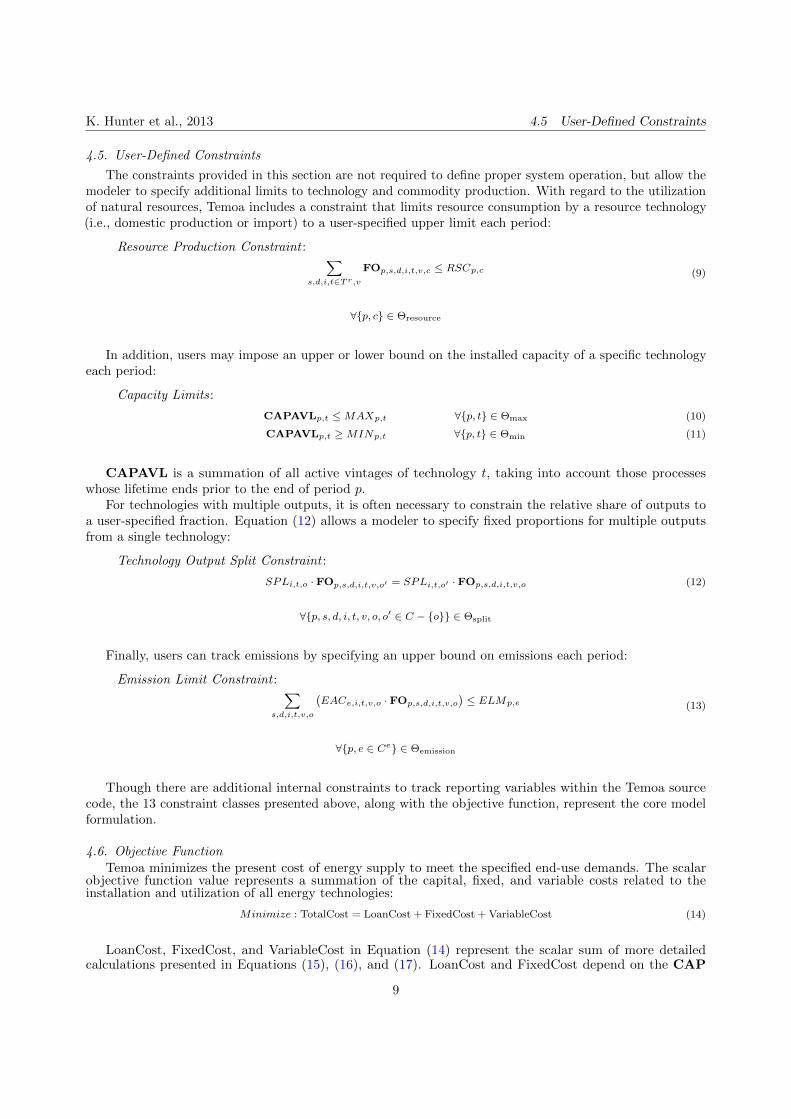
The constraints provided in this section are not required to define proper system operation, but allow themodeler to specify additional limits to technology and commodity production. With regard to the utilizationof natural resources, Temoa includes a constraint that limits resource consumption by a resource technology(i.e., domestic production or import) to a user-specified upper limit each period:

Resource Production Constraint : ∑s,d,i,t∈Tr,v

FOp,s,d,i,t,v,c ≤ RSCp,c (9)

∀{p, c} ∈ Θresource

In addition, users may impose an upper or lower bound on the installed capacity of a specific technologyeach period:

Capacity Limits:

CAPAVLp,t ≤MAXp,t ∀{p, t} ∈ Θmax (10)

CAPAVLp,t ≥MINp,t ∀{p, t} ∈ Θmin (11)

CAPAVL is a summation of all active vintages of technology t, taking into account those processeswhose lifetime ends prior to the end of period p.

For technologies with multiple outputs, it is often necessary to constrain the relative share of outputs toa user-specified fraction. Equation (12) allows a modeler to specify fixed proportions for multiple outputsfrom a single technology:

Technology Output Split Constraint :

SPLi,t,o · FOp,s,d,i,t,v,o′ = SPLi,t,o′ · FOp,s,d,i,t,v,o (12)

∀{p, s, d, i, t, v, o, o′ ∈ C − {o}} ∈ Θsplit

Finally, users can track emissions by specifying an upper bound on emissions each period:

Emission Limit Constraint : ∑s,d,i,t,v,o

(EACe,i,t,v,o · FOp,s,d,i,t,v,o

)≤ ELMp,e (13)

∀{p, e ∈ Ce} ∈ Θemission

Though there are additional internal constraints to track reporting variables within the Temoa sourcecode, the 13 constraint classes presented above, along with the objective function, represent the core modelformulation.

4.6. Objective Function

Temoa minimizes the present cost of energy supply to meet the specified end-use demands. The scalarobjective function value represents a summation of the capital, fixed, and variable costs related to theinstallation and utilization of all energy technologies:

Minimize : TotalCost = LoanCost + FixedCost + VariableCost (14)

LoanCost, FixedCost, and VariableCost in Equation (14) represent the scalar sum of more detailedcalculations presented in Equations (15), (16), and (17). LoanCost and FixedCost depend on the CAP

9

K. Hunter et al., 2013

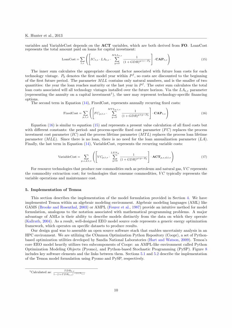
variables and VariableCost depends on the ACT variables, which are both derived from FO. LoanCostrepresents the total amount paid on loans for capital investment:

LoanCost =∑t,v

ICt,v · LAt,v ·MLLt,v∑

y=0

1

(1 + GDR)y+v−P0

·CAPt,v

(15)

The inner sum calculates the appropriate discount factor associated with future loan costs for eachtechnology vintage. P0 denotes the first model year within P f , so costs are discounted to the beginningof the first future period. The parameter MLL contains only natural numbers, and is the smaller of twoquantities: the year the loan reaches maturity or the last year in P f . The outer sum calculates the totalloan costs associated will all technology vintages installed over the future horizon. Via the LAt,v parameter(representing the annuity on a capital investment1), the user may represent technology-specific financingoptions.

The second term in Equation (14), FixedCost, represents annually recurring fixed costs:

FixedCost =∑p,t,v

FCp,t,v ·MTLp,t,v∑

y=0

1

(1 + GDR)y+p−P0

·CAPt,v

(16)

Equation (16) is similar to equation (15) and represents a present value calculation of all fixed costs butwith different constants: the period- and process-specific fixed cost parameter (FC) replaces the processinvestment cost parameter (IC) and the process lifetime parameter (MTL) replaces the process loan lifetimeparameter (MLL). Since there is no loan, there is no need for the loan annualization parameter (LA).Finally, the last term in Equation (14), VariableCost, represents the recurring variable costs:

VariableCost =∑

p,s,d,t,v

V Cp,t,v ·LENp∑y=0

1

(1 + GDR)y+p−P0

·ACTp,s,d,t,v

(17)

For resource technologies that produce raw commodities such as petroleum and natural gas, V C representsthe commodity extraction cost; for technologies that consume commodities, V C typically represents thevariable operations and maintenance cost.

5. Implementation of Temoa

This section describes the implementation of the model formulation provided in Section 4. We haveimplemented Temoa within an algebraic modeling environment. Algebraic modeling languages (AML) likeGAMS (Brooke and Rosenthal, 2003) or AMPL (Fourer et al., 1987) provide an intuitive method for modelformulation, analogous to the notation associated with mathematical programming problems. A majoradvantage of AMLs is their ability to describe models distinctly from the data on which they operate(Kallrath, 2004). As a result, well-designed EEO model source code represents a generic energy optimizationframework, which operates on specific datasets to produce results.

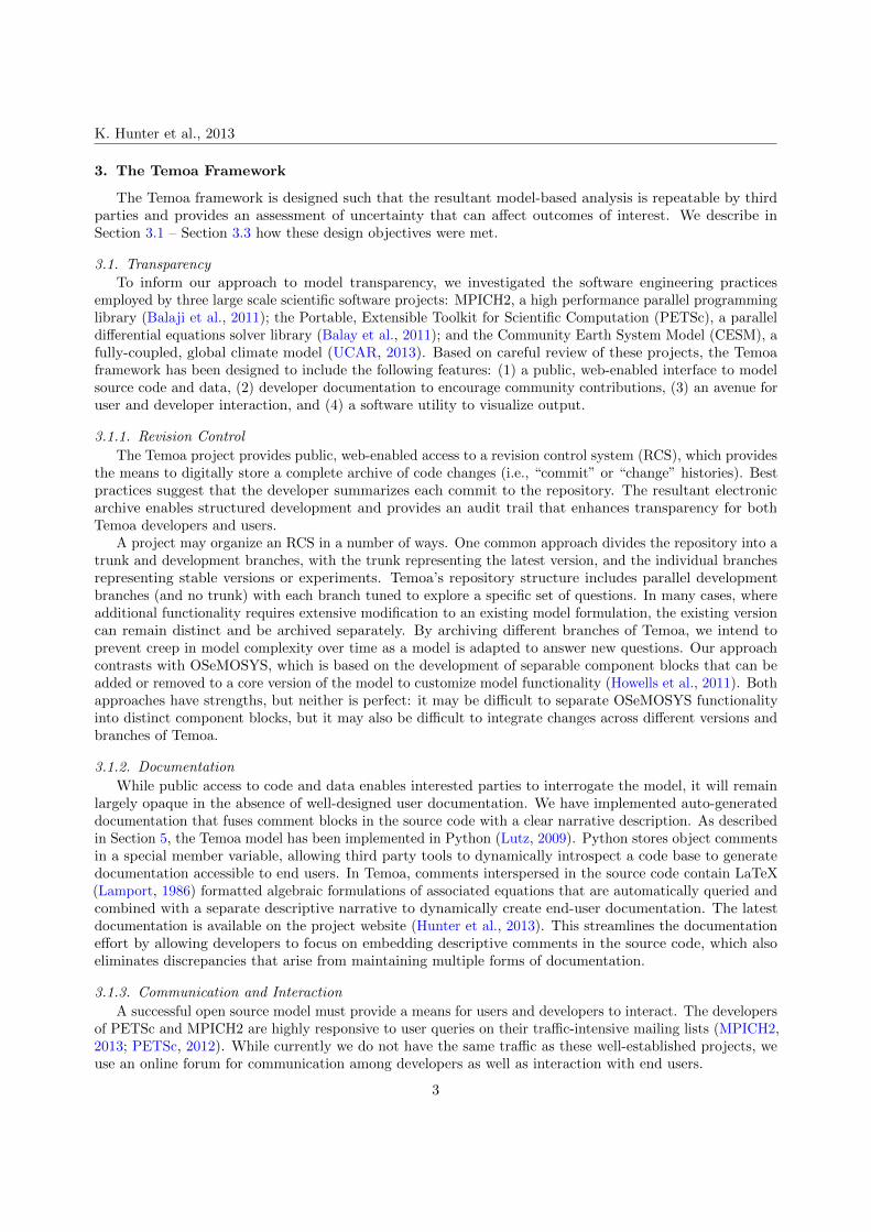
Our design goal was to assemble an open source software stack that enables uncertainty analysis in anHPC environment. We are utilizing the COmmon Optimization Python Repository (Coopr), a set of Python-based optimization utilities developed by Sandia National Laboratories (Hart and Watson, 2009). Temoa’score EEO model heavily utilizes two subcomponents of Coopr: an AMPL-like environment called PythonOptimization Modeling Objects (Pyomo), and Python-based Stochastic Programming (PySP). Figure 8includes key software elements and the links between them. Sections 5.1 and 5.2 describe the implementationof the Temoa model formulation using Pyomo and PySP, respectively.

1Calculated as:TDRt,v

1−(1+TDRt,v)−LLNt,v

10

K. Hunter et al., 2013 5.1 Programming Environment

5.1. Programming Environment

The choice of application programmer interface (API) and environment is crucial to a project whosestated goal is transparency. We selected Pyomo for a number of reasons. Influenced by the design of AMPL,Pyomo is an open source Python library that provides capabilities commonly associated with algebraicmodeling languages (AMLs) such as AMPL, AIMMS, and GAMS; however, Pyomo is also embedded withina full-featured high-level programming language with a rich set of supporting libraries (Hart, 2009). Pyomoleverages the Python component architecture to support extensibility in a modular manner. Modeling ina high level language allows modelers to utilize modern programming constructs, ensure cross-platformportability, and access the broad range of functionality found in standard software libraries. The benefits ofusing Python are twofold: (1) it serves as a robust, well-tested foundation for model development and (2)extensions generally require new classes or routines rather than changes to the language itself (Hart, 2009).

One drawback to Python and Pyomo over a standard AML is the verbosity of syntax. While a pure AMLhas syntax very close to actual mathematical notation, the generality of Python requires more overheadcode (i.e., required code that does not directly relate to the math). We made the decision to sacrifice theconciseness of an AML for the power and flexibility of a general purpose programming language. Python iswidely used in the scientific community (Perez et al., 2011) and such broad familiarity with Python is animportant consideration for a new modeling effort trying to appeal to modelers from a variety of disciplines.In addition, the algebraic formulation provided in Section 4 can be ported to a different programmingenvironment in the future, if necessary.

The Temoa user documentation made available on the project website describes the model implementationin detail (Hunter et al., 2013). To encourage contributions back to the energy modeling community, all ofTemoa’s model-specific code is made available under the GNU Affero Public License (FSF, 2007).

5.2. Optimization Tools

A key strength of Coopr is that models developed in Pyomo can link to optimizers written in low-levellanguages (e.g., C and FORTRAN). This two-language approach leverages the flexibility of a high-levellanguage for formulating optimization problems and the efficiency of low-level languages for numericalcomputations (Hart, 2009). Coopr links to several linear and mixed integer linear solvers, including CPLEX(Cplex, 2007), Gurobi (Bixby et al., 2010), CBC (Forrest and Lougee-Heimer, 2005), and GLPK (Makhorin,2010).

Another strategic reason for using Coopr is the ability to link Temoa with solvers that can handle avariety of mixed integer and non-linear formulations. Future Temoa development may include a mixed integeror non-linear formulation to model endogenous technological change (Barreto, 2001; Manne and Barreto,2004), non-linear macroeconomic production functions (e.g., Bauer et al., 2008), or use of the logit functionas a market sharing algorithm (Short et al., 2007).

Coopr also contains Python-based Stochastic Programming (PySP), a modeling and solver library forgeneric stochastic programming (Watson et al., 2010). Modeling in PySP involves coupling a fully-specifiedevent tree with a Pyomo-based deterministic, single-scenario model of the problem. The event tree specificationincludes the assignment of conditional probabilities and stochastic parameter values to each branch in theevent tree.

PySP can also address instances where the extensive form is too difficult to solve, due either to thepresence of integers (in any stage) or a sufficiently large event tree. In this case, PySP provides a genericand highly customizable scenario-based decomposition solver based on Rockafellar and Wets’ ProgressiveHedging algorithm, which has proved effective as a heuristic for difficult, multi-stage stochastic mixed-integerprograms (Rockafellar and Wets, 1991). Because the progressive hedging algorithm decomposes a stochasticproblem into the set of paths through the event tree, it is possible to implement the algorithm in a parallelcomputing environment.

6. Verification Exercise

With the algebraic model formulation and subsequent Pyomo implementation complete, we conducteda verification exercise to test model performance. Following the lead of Howells et al. (2011), we utilized

11

K. Hunter et al., 2013

‘Utopia’, a simple test energy system bundled with ANSWER, a graphical user interface packaged withthe MARKAL model generator (Noble, 2007). Utopia can deploy 17 technologies across three model timeperiods (1990, 2000, 2010) to meet 3 end-use demands: residential lighting (RL), residential space heating(RH), and automobile transportation (TX). Within each time period, a representative year is split into threeseasons (winter, summer, intermediate) and two times of day (day, night). Among the three seasons, theaverage lighting and space heating demands are highest in the winter and higher in the day compared tonight. Transportation demand remains constant throughout the year.

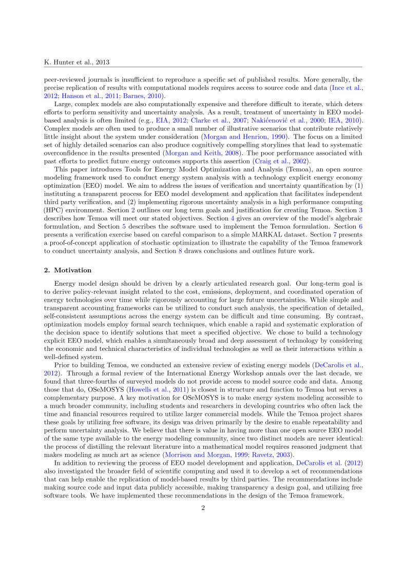
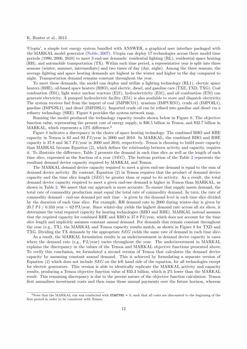
To meet these demands, the model can deploy and utilize a lighting technology (RL1), electric spaceheaters (RHE), oil-based space heaters (RHO), and electric, diesel, and gasoline cars (TXE, TXD, TXG). Coalcombustion (E01), light water nuclear reactors (E21), hydroelectricity (E31), and oil combustion (E70) cangenerate electricity. A pumped hydroelectric facility (E51) is also available to store and dispatch electricity.The system receives fuel from the import of coal (IMPHCO1), uranium (IMPURN1), crude oil (IMPOIL1),gasoline (IMPGSL1), and diesel (IMPDSL1). Imported crude oil can be refined into gasoline and diesel via arefinery technology (SRE). Figure 8 provides the system network map.

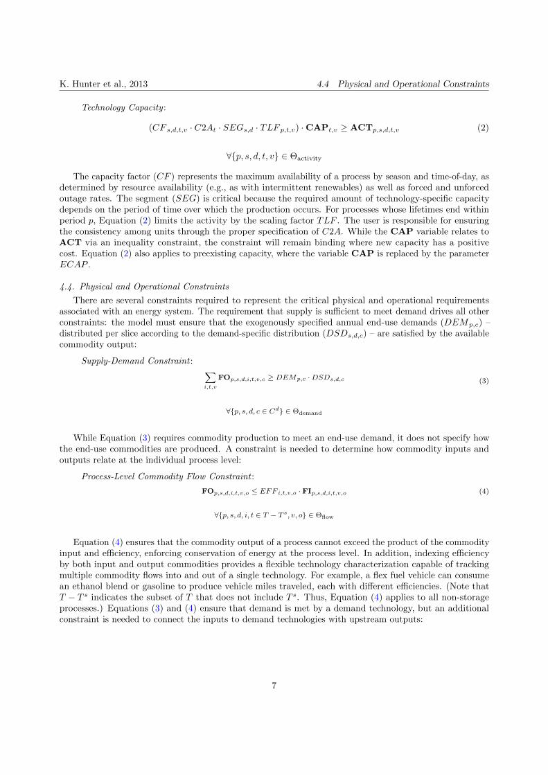
Running the model produced the technology capacity results shown below in Figure 8. The objectivefunction value, representing the present cost of energy supply, is $36.5 billion in Temoa, and $32.7 billion inMARKAL, which represents a 12% difference.2

Figure 8 indicates a discrepancy in the choice of space heating technology. The combined RHO and RHEcapacity in Temoa is 62 and 93 PJ/year in 2000 and 2010. In MARKAL, the combined RHO and RHEcapacity is 37.8 and 56.7 PJ/year in 2000 and 2010, respectively. Temoa is choosing to build more capacitythan MARKAL because Equation (2), which defines the relationship between activity and capacity, requiresit. To illustrate the difference, Table 2 presents the demand in each time slice as well as the length of eachtime slice, expressed as the fraction of a year (SEG). The bottom portion of the Table 2 represents theresultant demand device capacity required by MARKAL and Temoa.

The MARKAL demand device capacity required to meet a given end-use demand is equal to the sum ofdemand device activity. By contrast, Equation (2) in Temoa requires that the product of demand devicecapacity and the time slice length (SEG) be greater than or equal to its activity. As a result, the totaldemand device capacity required to meet a given end-use demand is higher in Temoa than MARKAL, asshown in Table 2. We assert that our approach is more accurate: To ensure that supply meets demand, thetotal rate of commodity production must equal the total rate of commodity demand. In turn, the rate ofcommodity demand – end-use demand per unit time – is given by the demand level in each time slice dividedby the duration of each time slice. For example, RH demand rate in 2000 during winter-day is given by20.7 PJ / 0.333 year = 62 PJ/year. Since winter-day yields the highest demand rate across all six slices, itdetermines the total required capacity for heating technologies (RHO and RHE). MARKAL instead assumesthat the required capacity for combined RHE and RHO is 37.8 PJ/year, which does not account for the timeslice length and implicitly assumes constant annual demand. For demands that remain constant throughoutthe year (e.g., TX), the MARKAL and Temoa capacity results match, as shown in Figure 8 for TXD andTXG. Dividing the TX demands by the appropriate SEG yields the same rate of demand in each time slice.

As a result, the MARKAL formulation results in an underinvestment in demand device capacity in caseswhere the demand rate (e.g., PJ/year) varies throughout the year. The underinvestment in MARKALexplains the discrepancy in the values of the Temoa and MARKAL objective functions presented above.To verify this conclusion, we formulated a second version of Temoa that calculates the demand devicecapacity by assuming constant annual demand. This is achieved by formulating a separate version ofEquation (2) which does not include SEG on the left hand side of the equation, for all technologies exceptfor electric generators. This version is able to identically replicate the MARKAL activity and capacityresults, producing a Temoa objective function value of $33.3 billion, which is 2% lower than the MARKALresult. This remaining discrepancy is due to the precise nature of the objective function calculation: Temoafirst annualizes investment costs and then sums those annual payments over the future horizon, whereas

2Note that the MARKAL run was conducted with STARTYRS = 0, such that all costs are discounted to the beginning of thefirst period in order to be consistent with Temoa.

12

K. Hunter et al., 2013

MARKAL assumes a lump sum investment cost, with a salvage value credited back to the objective functionfor capacity exceeding the specified future horizon.

The model source code and data used to generate results associated with the Utopia verification exerciseare archived in our Git repository, accessible from the project website (Hunter et al., 2013). Note that theTemoa formulation resides in the energysystem branch, while the alternative formulation used to replicatethe MARKAL result is archived separately in the exp energysystem match MARKAL branch.

7. Stochastic Implementation of Utopia

Upon completion of the verification exercise, we tested the functionality of PySP by implementing astochastic version of the Utopia system. The simplicity of the Utopia system and our familiarity with itthrough the model verification process made it a logical choice as a proof-of-concept test of Temoa’s stochasticoptimization capability. Suppose that Utopia is an island state and is gravely concerned with fuel supplyover the next three decades. Due to geopolitical concerns and a lack of domestic resources, the prices ofimported crude oil, diesel, gasoline, and coal are expected to increase dramatically from 2000 through 2019,corresponding to the 2000 and 2010 model time periods. Energy planners in Utopia would like to prepare astrategy that is contingent on the possible future price rates. The crude oil, diesel, and gasoline are importedfrom the same location, and therefore the low, medium, and high growth rates for all three fuels are assumedto be the same and follow identical growth patterns. The assumed import price growth rates are provided inTable 3.

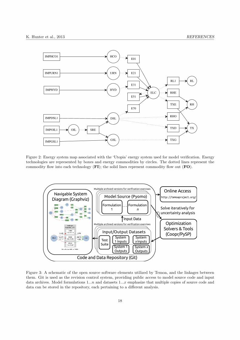
The resultant event tree considers each combination of growth rates for coal and liquid fuels, resultingin 9 branches per node implemented across two time stages with uncertainty for a total of 81 scenarios.For simplicity, each branch is assigned an equal probability of (1/9), or roughly 11%. The deterministicversion of the model (i.e., source code and base case data file) along with the event tree information waspassed to PySP, which constructed the extensive form of the stochastic problem and invoked CPLEX to findthe optimal solution. Figure 8 is a scatterplot of the total discounted system cost – the objective functionvalue – as a function of the average coal price from 2000 to 2019. The marker shading is proportional to theimported price of oil, diesel, and gasoline, where lighter shades indicate higher prices. Figure 8 indicates howtotal energy expenditures in Utopia vary under the 81 different fuel price scenarios.

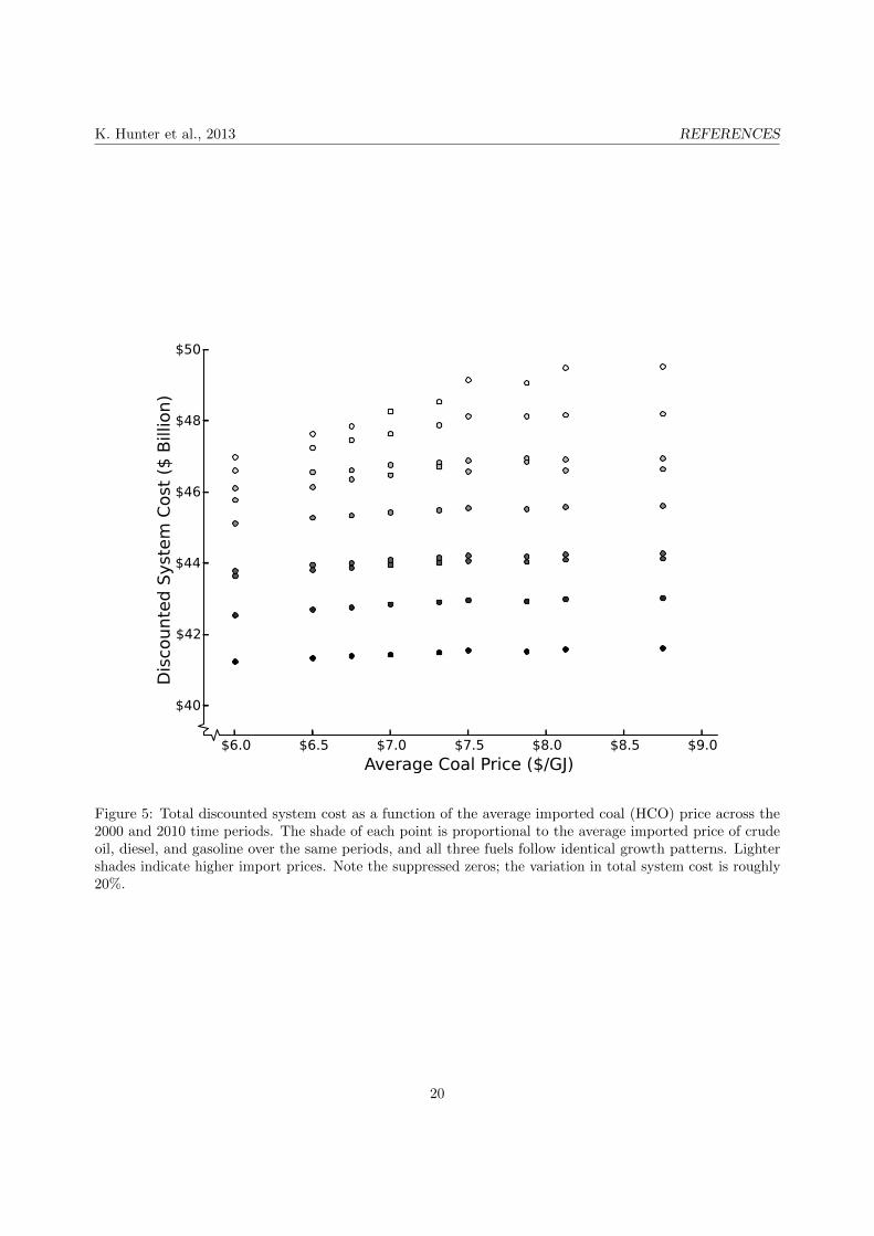
The variation in results can be observed by choosing two extreme scenarios within the event tree andexamining the technology results. Figure 8 provides the activity associated with both fuel imports anddemand devices in the Utopia system when coal prices are highest and liquid fuel prices are lowest (left bars),and vice versa (right bars). Since there is no modeled uncertainty in 1990, the results in all scenarios are thesame and represent a near-term hedging strategy that accounts for the modeled future outcomes weightedby their probabilities. The 1990 results indicate that Utopia should maintain a balance between imports ofcoal, diesel, and gasoline, with coal used for electricity generation (E01), diesel for space heating (RHO), andgasoline for vehicles (TXG). If coal prices remain high relative to imported oil, diesel, and gasoline prices, asin the left bars of Figure 8, Utopia should consider fuel switching in its electric sector to nuclear by 2010. Ifcoal prices are low relative to imported oil, diesel, and gasoline prices, as in the right bars of Figure 8, Utopiashould consider a sharp increase in coal imports in order to ramp up electricity production. The additionalelectricity can be used to supplant oil heaters (RHO) with electric heaters (RHE) and to displace a portionof the gasoline vehicles (TXG) with electric vehicles (TXE). The hedging strategy suggests a moderatedapproach to fuel imports in 1990, followed by recourse options over the following two decades depending onhow uncertainty in fuel prices imports are revealed.

While this stochastic exercise with Utopia is simply a proof-of-concept for the Temoa framework, theability to conduct stochastic optimization with much larger datasets in an HPC environment can lendvaluable insight into the planning process by allowing the construction of complex event trees that account formultiple parameter uncertainties. Note that Temoa’s stochastic version of Utopia draws on the source codeand data available in the energysystem branch, supplemented with files made available in the stochastic

subdirectory.

13

K. Hunter et al., 2013

8. Discussion

Two primary needs drive the design of Temoa: greater transparency in EEO modeling and rigorousassessment of future uncertainty. Towards transparency, Temoa draws on a large, existing ecosystem of opensource software components, and is itself an open source project. Temoa utilizes an open source AML-likeenvironment, Pyomo, to implement the algebraic formulation, links to open source solvers (e.g., GLPK),and is archived in an electronically and publically accessible RCS. The use of Pyomo allows us to conductsensitivity and uncertainty analysis in a HPC environment, thereby enabling parallel processing of modelruns required for parametric sensitivity analysis, Monte Carlo simulation, and stochastic optimization (viaPySP). In particular, the ability to conduct stochastic optimization with more complex event trees can betterinform decision makers who must take action on energy and environmental issues before future uncertaintyis resolved.

The verification exercise using the ‘Utopia’ system presented in Section 6 demonstrates that the Temoamodel formulation and implementation are correct. The observed discrepancy between MARKAL and Temoaregarding the calculation of demand device capacity demonstrates the utility of careful verification exercises.The comparison unearthed a simplification in the MARKAL formulation that can lead to underinvestment intechnology capacity. Despite its simplicity, the stochastic optimization of Utopia represents a proof-of-conceptapplication of Temoa. Further, public access to our RCS allows interested parties to use the archivedmodel source code and data, and more importantly, to reproduce our published results. For example, thoseinterested in reproducing our Utopia results can access a snapshot of the source code and data within theweb accessible repository, linked from the Temoa Project website (Hunter et al., 2013).

Over time, we fully expect that changes will be made to the model formulation. The formulation presentedhere represents a single snapshot archived in our publicly accessible RCS, but as we update the formulation,changes will be integrated into the documentation available on the project website. In addition, we plan touse the RCS to archive distinct versions of the model formulation with different capabilities, tuned to theneeds of particular analyses. Keeping the model codebase as small as possible for a particular application willmaintain model transparency by allowing modelers and users to interrogate model source code and data withgreater ease. While the implementation in Pyomo is more verbose than other algebraic modeling languagessuch as GAMS or AMPL, we hope that Temoa will benefit the energy modeling community.

Ongoing work by the authors is focused on methodological improvements in the application of stochasticoptimization, while external collaborators at Carnegie Mellon and Princeton Universities are conductingstudies related to U.S. natural gas supply, energy development on an American Indian reservation, andenergy futures in India.

Acknowledgments

This material is based upon work supported by the National Science Foundation under Grant No.(1055622).

References

Babonneau, F., Haurie, A., Loulou, R., Vielle, M., 2012. Combining Stochastic Optimization and Monte Carlo Simulation toDeal with Uncertainties in Climate Policy Assessment. Environmental Modeling and Assessment, 1–26.

Balaji, P., Buntinas, D., Butler, R., Chan, A., Goodell, D., Gropp, W., Krishna, J., Latham, R., Lusk, E., Mercier, G., Ross, R.,Thakur, R., 2011. MPICH2 User’s Guide. Tech. Rep. Version 1.4.1, Argonne National Laboratory, Office of Science, U.S.Department of Energy.

Balay, S., Brown, J., Buschelman, K., Eijkhout, V., Gropp, W. D., Kaushik, D., Knepley, M. G., McInnes, L. C., Smith, B. F.,Zhang, H., 2011. PETSc Users Manual. Tech. Rep. ANL-95/11 - Revision 3.2, Argonne National Laboratory.

Barnes, N., 2010. Publish Your Computer Code: It Is Good Enough. Nature 467 (7317), 753–753.Barreto, L., 2001. Technological Learning in Energy Optimisation Models and Deployment of Emerging Technologies. Ph.D.

thesis, National University.Bauer, N., Edenhofer, O., Kypreos, S., 2008. Linking Energy System and Macroeconomic Growth Models. Computational

Management Science 5 (1), 95–117.Bhatt, V., Friley, P., Lee, J., 2010. Integrated Energy and Environmental Systems Analysis Methodology for Achieving Low

Carbon Cities. Journal of Renewable and Sustainable Energy 2 (03).

14

K. Hunter et al., 2013 REFERENCES

Bixby, R., Gu, Z., Rothberg, E., 2010. Gurobi Optimization.Bosetti, V., Tavoni, M., 2009. Uncertain R&D, Backstop Technology and GHGs Stabilization. Energy Economics 31, S18–S26.Brooke, A., Rosenthal, R. E., 2003. GAMS. GAMS Development.Clarke, L., Edmonds, J., Jacoby, H., Pitcher, H., Reilly, J., Richels, R., Jul 2007. Scenarios of Greenhouse Gas Emissions and

Atmospheric Concentrations. U.S. Department of Energy Publications.URL http://digitalcommons.unl.edu/usdoepub/6

Cplex, I., 2007. 11.0 User’s Manual. ILOG SA:.Craig, P. P., Gadgil, A., Koomey, J. G., 2002. What Can History Teach Us? A Retrospective Examination of Long-Term Energy

Forecasts for the United States. Annual Review of Energy and the Environment 27 (1), 83–118.DeCarolis, J. F., 2011. Using Modeling to Generate Alternatives (MGA) to Expand Our Thinking on Energy Futures. Energy

Economics 33 (2), 145–152.DeCarolis, J. F., Hunter, K., Sreepathi, S., Jul 2012. The Case for Repeatable Analysis with Energy Economy Optimization

Models. Energy Economics 34 (6), 1845–1853.EIA, 2012. Annual Energy Outlook 2012. Tech. Rep. DOE/EIA-0383(2012), Office of Integrated Analysis and Forecasting, U.S.

Department of Energy, U.S. Government Printing Office, Washington, D.C., U.S. Energy Information Administration (EIA).Ellson, J., Gansner, E., Koutsofios, L., North, S., Woodhull, G., 2002. Graphviz – Open Source Graph Drawing Tools. In:

Graph Drawing. pp. 594–597.Fishbone, L. G., Abilock, H., Jan 1981. MARKAL, a Linear Programming Model for Energy Systems Analysis: Technical

Description of the BNL Version. International Journal of Energy Research 5 (4), 353–375.Forrest, J., Lougee-Heimer, R., 2005. Cbc user guide. INFORMS Tutorials in Operations Research, 257–277.Fourer, R., Gay, D. M., Kernighan, B. W., 1987. AMPL: A Mathematical Programming Language. AT&T Bell Laboratories.FSF, Nov 2007. GNU Affero General Public License. Version 3. Free Software Foundation (FSF), Boston, MA, USA. (Accessed

Apr, 2013).URL https://www.gnu.org/licenses/agpl-3.0.html

Gritsevskyi, A., Nakicenovi, N., Nov 2000. Modeling Uncertainty of Induced Technological Change. Energy Policy 28 (13),907–921.

Hanson, B., Sugden, A., Alberts, B., 2011. Making Data Maximally Available. Science 331 (6018), 649–649.Hart, W. E., 2009. Python Optimization Modeling Objects (Pyomo). Operations Research and Cyber-Infrastructure, 3–19.Hart, W. E., Watson, J.-P., 2009. Coopr: a COmmon Optimization Python Repository Sandia National Laboratories,

Albuquerque, NM, USA.URL http://software.sandia.gov/coopr/

Holthausen, D. M., Dec 1979. Hedging and the Competitive Firm Under Price Uncertainty. The American Economic Review69 (5), 989–995.

Howells, M., Rogner, H., Strachan, N., Heaps, C., Huntington, H., Kypreos, S., Hughes, A., Silveira, S., DeCarolis, J., Bazillian,M., Roehrl, A., Oct 2011. OSeMOSYS: The Open Source Energy Modeling System: An Introduction to Its Ethos, Structureand Development. Energy Policy 39 (10), 5850–5870.

Hunter, K., DeCarolis, J., Sreepathi, S., 2013. Tools for Energy Modeling Optimization and Analysis. (website), (Accessed Apr,2013).URL http://temoaproject.org/

IEA, 2010. Energy Technology Perspectives 2010: Scenarios and Strategies to 2050. Organisation for Economic Cooperationand Development, Paris, France, OECD. Publishing and International Energy Agency.

Ince, D. C., Hatton, L., Graham-Cumming, J., 2012. The Case for Open Computer Programs. Nature 482 (7386), 485–488.Kainuma, M., Matsuoka, Y., Morita, T., 1998. Analysis of Post-Kyoto Scenarios: The AIM Model. In: Economic Modeling of

Climate Change: OECD Workshop Report.Kallrath, J., 2004. Modeling Languages in Mathematical Optimization. Vol. 88. Springer.Kann, A., Weyant, J. P., 2000. Approaches for Performing Uncertainty Analysis in Large-Scale Energy/Economic Policy Models.

Environmental Modeling & Assessment 5 (1), 29–46.Kanudia, A., Loulou, R., 1998. Robust Responses to Climate Change via Stochastic MARKAL: The Case of Quebec. European

Journal of Operational Research 106 (1), 15–30.Labriet, M., Loulou, R., Kanudia, A., d’etudes et de recherche en analyse des decisions (Montreal, Quebec), G., 2008. Is a 2

Degrees Celsius Warming Achievable Under High Uncertainty?: Analysis with the TIMES Integrated Assessment Model.Groupe d’etudes et de recherche en analyse des decisions.

Lamport, L., 1986. LaTeX: A Document Preparation System, 2nd Edition. Addison-Wesley Longman Publishing Co., Inc.,Boston, MA, USA.

Loulou, R., Goldstein, G., Noble, K., et al., 2004. Documentation for the MARKAL Family of Models. IEA Energy TechnologySystems Analysis Programme.

Loulou, R., Kanudia, A., 1999. Minimax Regret Strategies for Greenhouse Gas Abatement: Methodology and Application.Operations Research Letters 25 (5), 219–230.

Loulou, R., Lehtila, A., 2007. Stochastic Programming and Tradeoff Analysis in TIMES. IEA ETSAP TIMES version 2.Loulou, R., Remme, U., Kanudia, A., Lehtila, A., Goldstein, G., 2005. Documentation for the TIMES Model PART I. Energy

Technology Systems Analysis Programme. Disponıvel.Lutz, M., Sep 2009. Learning Python, 4th Edition. O’Reilly.Makhorin, A., 2010. GNU Linear Programming Kit: Reference Manual for GLPK Version 4.45 38, Department for Applied

Informatics, Moscow Aviation Institute. Moscow, Russia.Manne, A. S., Barreto, L., Jul 2004. Learn-by-Doing and Carbon Dioxide Abatement. Energy Economics 26 (4), 621–633.

15

K. Hunter et al., 2013 REFERENCES

Messner, S., Strubegger, M., 1995. User’s Guide for MESSAGE III. Rep. WP-95-69, International Institute for Applied SystemsAnalysis, Laxenburg, Austria.

Morgan, M. G., Henrion, M., 1990. Uncertainty: A Guide to Dealing with Uncertainty in Quantitative Risk and Policy Analysis.New York, New York, USA.

Morgan, M. G., Keith, D. W., 2008. Improving the Way We Think about Projecting Future Energy Use and Emissions ofCarbon Dioxide. Climatic Change 90 (3), 189–215.

Morris, S. C., Goldstein, G. A., Sanghi, A., Hill, D., 1996. Energy Demand and Supply in Metropolitan New York with GlobalClimate Change. Annals of the New York Academy of Sciences 790 (1), 139–150.

Morrison, M., Morgan, M. S., 1999. Models as Mediating Instruments. IDEAS IN CONTEXT 52, 10–37.MPICH2, Mar 2013. MPICH2. (webpage), (Accessed Apr, 2013).

URL http://www.mpich.org/

Nakicenovic, N., Alcamo, J., Davis, G., de Vries, B., Fenhann, J., Gaffin, S., Gregory, K., Grubler, A., Jung, T. Y., Kram, T.,et al., 2000. Special Report on Emissions Scenarios: A Special Report of Working Group III of the Intergovernmental Panelon Climate Change. Cambridge University Press, New York, NY (US), Pacific Northwest National Laboratory, Richland, WA(US), Environmental Molecular Sciences Laboratory (US).

Noble, K., 2007. ANSWER v6 MARKAL User Manual: ANSWER MARKAL, an Energy Policy Optimization Tool. Noble-SoftSystems Pty Ltd, Australia.

Nordhaus, W. D., 1993. Rolling the DICE’: An Optimal Transition Path for Controlling Greenhouse Gases. Resource andEnergy Economics 15 (1), 27–50.

Perez, F., Granger, B., Hunter, J., 2011. Python: An Ecosystem for Scientific Computing. Computing in Science & Engineering13 (2), 13–21.

PETSc, Jun 2012. Portable, Extensible Toolkit for Scientific Computation. (website), (Accessed Apr, 2013).URL http://www.mcs.anl.gov/petsc/

Ravetz, J., 2003. Models as Metaphors. Public Participation in Sustainability Science: A Handbook, 62Cambridge UniversityPress.

Rockafellar, R. T., Wets, R. J. B., 1991. Scenarios and Policy Aggregation in Optimization Under Uncertainty. Mathematics ofOperations Research, 119–147.

Short, W., Ferguson, T., Leifman, M., 2007. Modeling of Uncertainties in Major Drivers in US Electricity Markets. NREL.UCAR, Mar 2013. Community Earth System Model (CESM). (website), University Corporation for Atmospheric Research

(UCAR).URL http://www.cesm.ucar.edu/

Watson, J.-P., Woodruff, D. L., Jul 2010. Progressive Hedging Innovations for a Class of Stochastic Mixed-Integer ResourceAllocation Problems. Computational Management Science 8 (4), 355–370.

Watson, J. P., Woodruff, D. L., Hart, W. E., 2010. PySP: Modeling and Solving Stochastic Programs in Python. Tech. rep.,Technical report, Sandia National Laboratories, Albuquerque, NM, USA.

Weyant, J. P., 1993. Costs of Reducing Global Carbon Emissions. The Journal of Economic Perspectives 7 (4), 27–46.

16

K. Hunter et al., 2013 REFERENCES

Inability to validate

model results

Increasing availability of

data

+

+

+

Moore's Law

Increasing model

complexity

Lack of openness

Inability to verify model

results

Uncertainty analysis is difficult

Figure 1: Causal model that highlights the limitations associated with the prevailing approach to EEO modeldevelopment and application. The Temoa project aims to address the issues highlighted in gray.

17

K. Hunter et al., 2013 REFERENCES

E01

ELC

E21

E31

E51

E70

IMPDSL1 DSL

IMPGSL1 GSL

IMPHCO1 HCO

IMPHYD HYD

IMPOIL1 OIL

IMPURN1 URN

RHE

RH

RHO

RL1 RL

SRE TXD TX

TXE

TXG

Figure 2: Energy system map associated with the ‘Utopia’ energy system used for model verification. Energytechnologies are represented by boxes and energy commodities by circles. The dotted lines represent thecommodity flow into each technology (FI); the solid lines represent commodity flow out (FO).

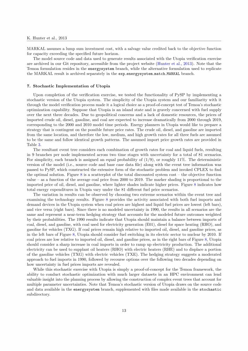
Figure 3: A schematic of the open source software elements utilized by Temoa, and the linkages betweenthem. Git is used as the revision control system, providing public access to model source code and inputdata archives. Model formulations 1...n and datasets 1...x emphasize that multiple copies of source code anddata can be stored in the repository, each pertaining to a different analysis.

18

K. Hunter et al., 2013 REFERENCES

0

20

40

60

80

100

120

Peta

joule

s/

Year

Import Technologies

IMPDSL1

IMPDSL1

IMPDSL1

IMPGSL1IMPGSL1 IMPGSL1

IMPHCO1

IMPHCO1

IMPHCO1

0.0

0.5

1.0

1.5

2.0

Gig

aw

att

s

Electric Generators

E01

E01E01

E31 E31 E31

E51 E51 E51E70 E70 E70

1990 2000 20100

10203040506070

Peta

joule

s/

Year

Demand Devices

RHE

RHE RHE

RHORHO

RHO

RL1RL1

RL1

TXD TXD TXDTXG TXG TXG

Figure 4: Technology capacity in each model time period for both MARKAL and Temoa using the ‘Utopia’test system. Black and white represent MARKAL and Temoa results, respectively. Names above each setof black-white bars indicate the technology name. Note that Temoa requires higher capacities for demanddevices serving end-use demands that vary by season and time-of-day. The difference in the required capacityfor demand devices drives the discrepancies in results between MARKAL and Temoa.

19

K. Hunter et al., 2013 REFERENCES

Figure 5: Total discounted system cost as a function of the average imported coal (HCO) price across the2000 and 2010 time periods. The shade of each point is proportional to the average imported price of crudeoil, diesel, and gasoline over the same periods, and all three fuels follow identical growth patterns. Lightershades indicate higher import prices. Note the suppressed zeros; the variation in total system cost is roughly20%.

20

K. Hunter et al., 2013 REFERENCES

0

50

100

150

200

250

Act

ivit

y (P

J/ye

ar)

IMPDSLIMPGSLIMPHCOIMPHYDIMPURNIMPOIL

1990 2000 2010Year

0

10

20

30

40

50

60

70

80

90

Act

ivit

y (P

J/ye

ar)

RHORL1TXDTXGRHETXE

Figure 6: Results associated with fuel imports (top) and the energy produced by demand devices (bottom)for two scenarios drawn from the stochastic Utopia run. For each time period, the left bars correspond tothe scenario with the highest coal prices and lowest oil, diesel, and gasoline prices; the right bars correspondto the scenario with the lowest coal prices and highest oil, diesel, and gasoline prices.

21

K. Hunter et al., 2013 REFERENCES

Table 1a: List and Description of Temoa’s Set Nomenclature

Set Short Descriptionc ∈ C C is the set of all user-defined commodities

Cd ⊂ CCd is a subset of (C) that includes only the demand commodities, i.e., the commoditiesrepresenting end-use demands

Ce ⊂ CCe is a subset of (C) that includes only the emissions commodities, i.e., the commoditiesrepresenting pollutant emissions

d ∈ D D is the set of all diurnal time segments (d)i = c i is an alias for c, representing the commodity input to a technologyo = c o is an alias for c, representing the commodity output from a technologyP e set of periods that define technology vintages existing prior to the future period set (P f )

p ∈ P f model periods of interest; each element marks the beginning of a period; the last elementspecifies the last year of the horizon, not the beginning of another period

v ∈ VV is the set of all technology vintages (v); a vintage is defined by the model time period(p) in which a technology (t) is installed; V = P e ∪ P f

s ∈ S S is the set of all user-defined seasons (s)t ∈ T T is the set of all user-defined technologies (t)

T b ⊂ TT b is a subset of (T ) that includes only baseload electric technologies, i.e., thermal powerplants that do not adjust output diurnally

T d ⊂ TT d is a subset of (T ) that includes only demand technologies, i.e., the technologies directlyserving an end-use demand.

T r ⊂ TT r is a subset of (T ) that includes only resource technologies, i.e., the technologies thatrepresent the extraction or import of natural resources

T s ⊂ TT s is a subset of (T ) that includes only the storage technologies, which balance storageand dispatch across the set of daily time segments (D)

ΘSparse superset representing allowable combinations of set elements. The subscript to Θuniquely identifies the superset associated with each equation.

Table 1b: List and Description of Temoa’s Parameter Nomenclature

Parameter Short DescriptionC2At,v parameter that converts capacity units to activity unitsCF s,d,t,v capacity factor of a process that can vary by season and time of dayDEMp,c end-use demands specified by period and commodityDSDs,d,c Percentage distribution of demand c, per time sliceEACe,i,t,v,o emissions rate of process based on input / output commodity pairECAP t,v amount of pre-existing process capacity prior to P f

EFF i,t,v,o conversion efficiency; based on input / output commodity pairELMp,e emissions limit specified per periodFCp,t,v fixed operations and maintenance costGDR global discount rate used to calculate present value of future period costsICt,v process investment cost

LAt,v

∗loan amortization factor to convert future lump sum investment costs to annualizedamounts; based on TDR

LENp∗calculated number of years in period p ∈ P f

LLNt,v∗process-specific loan term

MAXp,t upper bound on capacity installation by model time periodMINp,t lower bound on capacity installation by model time period

MLLt,v

∗lesser of the following: number of years until the end of process loan life or the finalyear in the P f horizon

MTLp,t,v

∗lesser of the following: number of years until the end of process lifetime or the final yearin the P f horizon

RSCp,c upper bound on resource commodity productionSEGs,d fraction of year represented by each combination of season (s) and time-of-day (d)

SPLi,t,ofraction of total input commodity (i) converted to the output commodity (o) throughtechnology (t)

TDRt,v technology-specific discount rate used to calculate LA. Defaults to GDR if not specifiedTLF p,t,v

∗fraction of period p that a process is activeV Cp,t,v variable cost

(∗) Temoa automatically determines the indices and values of these parameters.

22

K. Hunter et al., 2013 REFERENCES

Table 1c: List and Description of Temoa’s Variable Nomenclature

Variable Short DescriptionFIp,s,d,i,t,v,o commodity flow into a process to produce a given output, per time sliceFOp,s,d,i,t,v,o commodity flow out of a process based on a given input, per time sliceACTp,s,d,t,v total commodity production of a process, per time sliceCAPt,v process capacity required to support all associated activity

CAPAVLp,ttotal capacity available of technology t in period p; not necessarily a simple vintagesummation because of the TLF parameter

Table 2: Utopia Demand Data and MARKAL and Temoa Results

Time Slice SEGs,dRL RH TX

2000 2010 2000 2010 2000 2010Intermediate-Day 0.167 1.26 1.89 4.54 6.80 1.30 1.95Intermediate-Night 0.083 0.42 0.63 2.27 3.40 0.65 0.97Summer-Day 0.167 1.26 1.89 0 0 1.30 1.95Summer-Night 0.083 0.42 0.63 0 0 0.65 0.97Winter-Day 0.333 4.20 6.30 20.7 31.0 2.60 3.90Winter-Night 0.167 0.84 1.26 10.3 15.5 1.30 1.95MARKAL Capacity 8.40 12.6 37.8 56.7 7.80 11.69Temoa Capacity 12.6 18.9 62.0 93.0 7.80 11.69

Table 3: Decadal Growth Rates Used in Stochastic Utopia

Import Prices Low Medium HighCoal 200% 225% 250%Oil, Diesel, Gasoline 125% 150% 175%

23