Embed Size (px)
Citation preview
Research NoteNational Security Report
PARAMETRIC
MODELING FOR EARLY TECHNOLOGY DEVELOPMENT
COST AND SCHEDULE
Chuck Alexander
NSR_11x17_Cover_CostModeling_v8.indd 1 11/20/17 3:15 PM

PARAMETRIC COST AND SCHEDULE MODELING FOR EARLY TECHNOLOGY DEVELOPMENT
Chuck Alexander

Copyright © 2018 The Johns Hopkins University Applied Physics Laboratory LLC. All Rights Reserved.
Contact Chuck Alexander at [email protected] to request detailed model results.
This work was first presented at the International Cost Estimating & Analysis Association (ICEAA) 2017 Professional Development & Training Workshop in Portland, Oregon, June 6–9, 2017 (http://www.iceaaonline.com/portland2017/). It earned the workshop’s 2017 Best Paper in the Analysis Methods Category and 2017 Best Paper Overall awards. It was also presented at the 2017 NASA Cost and Schedule Symposium at NASA Headquarters on August 30, 2017.
NSAD-R-17-034
PARAMETRIC COST AND SCHEDULE MODELING FOR EARLY TECHNOLOGY DEVELOPMENT iii
Contents
Figures ................................................................................................................................................................................................ v
Tables ................................................................................................................................................................................................. vi
Summary ......................................................................................................................................................................................... vii
Background—Literature, Model, and Source Data Search ...............................................................................1
Data Resource ...........................................................................................................................................................2
Modeling Approach .................................................................................................................................................3
Key Data Selection .................................................................................................................................................................. 3
Data Modeling ......................................................................................................................................................................... 4
TRL Levels—Background ..................................................................................................................................................... 5
Preliminary Data Relationship Screening ....................................................................................................................... 6
Cost Forecast Models ............................................................................................................................................................. 7
Schedule Forecast Models ................................................................................................................................................... 7
Data Set Construction ........................................................................................................................................................... 8
Core Model Development ................................................................................................................................................... 9
Modeling Uncertainty .........................................................................................................................................................10
Model Selection Criteria—Measures of Performance .................................................................................... 10
Cost Model Performance ...................................................................................................................................... 11
Overall Results ........................................................................................................................................................................11
Curve Fit Cost Models ..........................................................................................................................................................13
Simple Linear Regression Cost Models .........................................................................................................................14
Multivariate Linear Regression Cost Models ...............................................................................................................14
Nonlinear Cost Models ........................................................................................................................................................16
Schedule Model Performance ............................................................................................................................. 17
Cost and Schedule Model Variability ................................................................................................................. 18
Conclusions and Future Work ............................................................................................................................. 19
THE JOHNS HOPKINS UNIVERSITY APPLIED PHYSICS LABORATORYiv
Appendix A Definitions ..........................................................................................................................................................23
Appendix B Preliminary Data Relationship Screening ................................................................................................25
Appendix C Technology Readiness Level (TRL) Start–End Cost Data ....................................................................33
Appendix D Technology Readiness Level (TRL) Start–End Duration Data ...........................................................37
Appendix E Key Performance Measure Descriptions ..................................................................................................41
Acknowledgments .......................................................................................................................................................................43
About the Author .........................................................................................................................................................................43
Bibliography ...................................................................................................................................................................................45
PARAMETRIC COST AND SCHEDULE MODELING FOR EARLY TECHNOLOGY DEVELOPMENT v
Figures
Figures
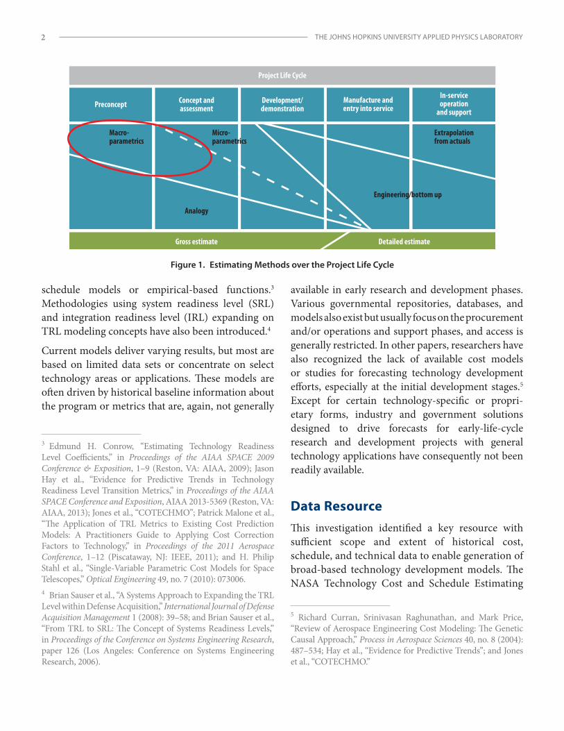
Figure 1. Estimating Methods over the Project Life Cycle .............................................................................................. 2
Figure 2. Average Total Development Costs vs. TI Level ................................................................................................. 7
Figure 3. Average Total Development Costs vs. SH Level ............................................................................................... 7
Figure 4. Average Project Duration vs. SH Level ................................................................................................................ 7
Figure 5. Average Project Duration vs. TI Level .................................................................................................................. 8
Figure 6. TI Sample Mean Cost vs. TI-Based Models .......................................................................................................12
Figure 7. SH Sample Mean Cost vs. SH-Based Models ...................................................................................................13
Figure 8. Example TI Cost Curve Fit Model No. 1—Cost (FY15$) for TI Level 1 .....................................................14
Figure 9. Example SH Cost Curve Fit Model No. 2—Cost (FY15$) for SH Level 1 .................................................14
Figure 10. Example Linear Regression Model PDFs for Model No. 5 SH Level 1 (Left) and Model No. 6 SH Level 2 (Right) ................................................................................................................................15
Figure 11. Model No. 9—Total Cost vs. f [TI Level + SH Level]2 ...................................................................................15
Figure 12. Cost Model No. 9—Example PDF for TI Level 1 and SH Level 5 ..............................................................16
Figure 13. SH Nonlinear Model Statistics Plot and Data Table ....................................................................................16
Figure 14. Cost Model No. 12—SH Level 1 Example ......................................................................................................16
Figure 15. Example Schedule Curve Fits and Selected PDF—Schedule Model No. 1 for SH Level 2, Project Duration (Months) ....................................................................................................................17
Figure 16. Schedule Model No. 1 (SH Curve Fit) Results —Project Duration (Months) ......................................18
Figure Credits:
Figure S-1/Figure 1: Dale Shermon and Catherine Barnaby, “Macro-Parametrics and the Applications of Multi-Colinearity and Bayesian to Enhance Early Cost Modeling,” in Proceedings of the International Cost Estimating and Analysis Association 2015 Professional Development & Training Workshop (Annandale, VA: ICEAA, 2015).
THE JOHNS HOPKINS UNIVERSITY APPLIED PHYSICS LABORATORYvi
Tables
Tables
Table 1. Cost Model KPM Results ...........................................................................................................................................12
Table 2. Summary Cost (FY15$) Curve Fit Model Statistics ..........................................................................................13
Table 3. Development Schedule Duration (Months) Curve Fit Model—Key Benchmark Data ......................17
Table 4. Model No. 1 (SH Curve Fit) KPM Results .............................................................................................................18
Table 5. General Cost Model Applicability .........................................................................................................................20
Table Credits:
Table A-1: Stuart K. Cole et al., Technology Estimating: A Process to Determine Cost and Schedule of Space Technology R&D, NASA/TP–2013-218145 (Washington, DC: NASA, 2013).
Table A-2: Adapted from NASA TRL Scale, “Technology Readiness Level,” October 28, 2012, https://www.nasa.gov/directorates/heo/scan/engineering/technology/txt_accordion1.html.
Table A-3: SpaceWorks Enterprises, Inc., TCASE Technology Cost and Schedule Estimation Tool User Training Presentation, Rev5 (2015-03-19) (Atlanta: SpaceWorks, 2015).
Table A-4: Cole et al., Technology Estimating.
PARAMETRIC COST AND SCHEDULE MODELING FOR EARLY TECHNOLOGY DEVELOPMENT vii
Summary
Estimating technology development in support of investment decisions continues to be a formidable challenge in the cost community. Design, performance, or technical requirements, which drive traditional parametric models or translate analogous system costs, are often unavailable in the early life-cycle stages of basic or applied technology development. Often compounding the limited availability of information about the technology is the proprietary or protected nature of technology research and development efforts and related intellectual property. Restrictions on sharing information contribute to the lack of data, objective models, and methods that can be broadly applied in early planning stages.
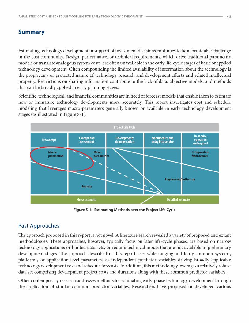
Scientific, technological, and financial communities are in need of forecast models that enable them to estimate new or immature technology developments more accurately. This report investigates cost and schedule modeling that leverages macro-parameters generally known or available in early technology development stages (as illustrated in Figure S-1).
Project Life Cycle
Preconcept
Macro-parametrics
Analogy
Micro-parametrics
Extrapolationfrom actuals
Detailed estimateGross estimate
Concept andassessment
Development/demonstration
Manufacture andentry into service
In-serviceoperation
and support
Engineering/bottom up
Figure S-1. Estimating Methods over the Project Life Cycle
Past Approaches
The approach proposed in this report is not novel. A literature search revealed a variety of proposed and extant methodologies. These approaches, however, typically focus on later life-cycle phases, are based on narrow technology applications or limited data sets, or require technical inputs that are not available in preliminary development stages. The approach described in this report uses wide-ranging and fairly common system-, platform-, or application-level parameters as independent predictor variables driving broadly applicable technology development cost and schedule forecasts. In addition, this methodology leverages a relatively robust data set comprising development project costs and durations along with these common predictor variables.
Other contemporary research addresses methods for estimating early-phase technology development through the application of similar common predictor variables. Researchers have proposed or developed various
THE JOHNS HOPKINS UNIVERSITY APPLIED PHYSICS LABORATORYviii
frameworks, analyses, and modeling concepts that apply predictors such as technology readiness levels (TRL), system readiness levels (SRL), and integration readiness levels (IRL). These models deliver varying results, but most are based on limited data sets, concentrate on select technology areas or applications, and often require historical baseline information about the program that is, again, generally unavailable in early research and development phases.
Modeling Methodology
The author identified the NASA Technology Cost and Schedule Estimating (TCASE) tool as a resource with the desired scope and magnitude of historical cost, schedule, and technical data. TCASE was introduced by the Cost Analysis Division at NASA Headquarters, along with SpaceWorks Enterprises, Inc., in early 2013. At the core of this tool is an extensive technology database containing over 2,900 project records. These records cover fourteen wide-ranging technology areas and a broad scope of applications and systems that are relevant across the scientific, military, and intelligence sectors.
The goal of the research was to identify causal variables with which to produce viable models for estimating a project’s cost and duration. The author evaluated several data fields as potential predictor variables, including system hierarchy (SH) level (1–5); TRL at the project’s start and completion (1–9); research and development degree of difficulty (RD3) (levels I–V); technology area (TA1–TA14); key performance parameters; total full-time equivalents (FTEs) of project labor; capability demonstrations; and certain system characteristics. However, due largely to limited data field records, predictor variable selections had to be restricted to two measures: TRL and SH.
Parsing the TRL start and end (TRL X–Y) metrics and assessing initial data relationship screening (see Appendix B) revealed that the quantity of available data points was inadequate to provide the statistical significance required. Instead, the author investigated a different metric, namely TRL level improvement from a project’s start and end, often referred to as the TRL transition metric. The author selected TRL improvement (TI) level, measured as the project’s net TRL level increase over its development time frame, based on this metric’s improved sample sizes and initial screening results. This analysis revealed that nonlinear behavior was evident in both TI and SH cost and schedule relationships.
To provide a diversity of perspectives for cost and schedule estimating, the author examined a comprehensive set of model forms, including tailored curve fit models, simple and multiple regression models, and a range of nonlinear models. The author also explored various data transformations for all regression models. The author then applied model selection criteria to model results, including a comprehensive set of statistical key performance measures (KPMs), additional measures tailored or relevant to particular model forms, and an overall assessment of the goodness of fit to sample data.
Model Performance Results
The author evaluated several hundred cost models, with a few curve fit and multiple regression models providing the best results. Research determined that SH level appears to impact cost somewhat moderately up to SH level 4, above which point the impact becomes prominent. Therefore, for system-level technology developments, models containing the SH level variable are most suitable. Below the system level, the TI level is more dominant, and models containing the TI level parameter will more effectively explain model response
PARAMETRIC COST AND SCHEDULE MODELING FOR EARLY TECHNOLOGY DEVELOPMENT ix
behavior. However, if planned SH and TI levels are known, multivariate models applying both predictor variables may improve model performance, since these variables address both scalar (including scalar complexity) and technical dimensions. Schedule modeling produced more limited results, with effective SH-based duration curve fits.
Future Work
If the TCASE database can be expanded or other data sources leveraged for key response and predictor variables like RD3, technology area, and capability demonstrations, model functionality and accuracy might be improved and output variability reduced. In addition, other macro cost and schedule parameters that may augment forecasting in early-stage technology development include advanced degree of difficulty; SRL; IRL; implementation readiness level; and manufacturing readiness level. Broad-based technology performance or complexity factors, however, may hold the greatest potential to complement the models presented in this report. Leveraging these types of metrics to better integrate cost and schedule modeling with technology road mapping, early systems engineering, and conceptual design efforts should help generate more consistent development estimates. More accurate and consistent estimates can further lead to better investment and design decisions with greater cost impact early in the project life cycle.

PARAMETRIC COST AND SCHEDULE MODELING FOR EARLY TECHNOLOGY DEVELOPMENT 1
Industry and government models, tools, and contemporary research were explored for solutions to formulate cost and schedule
estimates that enhance investment decision-making in early-stage technology development. This investigation revealed a variety of proposed and existing methodologies. These solutions, however, focus on later phases in the project life cycle, are based on narrow technology applications and limited data sets, or require technical inputs that are typically not available in preliminary development stages. Estimators need common or wide-ranging system-, platform-, or application-level parameters to serve as independent predictor variables and drive cost and schedule forecasts when little engineering or performance information is available, potentially even before conceptual design has commenced. Therefore, the investigation included a search for applicable source data and modeling approaches to address a range of technologies applying macro-level cost and schedule drivers available in the initial planning and research stages of a development program. This examination was intended to assess existing solutions as well as to identify a relevant data set, select parameters, and develop methodologies to produce viable models for broad-based estimating early in the technology development life cycle.
Background—Literature, Model, and Source Data SearchIn preconceptual and early conceptual stages of a development project, design and performance information typically applied in traditional parametric cost and schedule models is usually very limited. Key attributes of such models often focus on subsystem- or unit/assembly-level characteristics or performance metrics that have not yet been determined in these preliminary stages. Therefore, macro-level parameters must be applied at a broader system or platform level. Investigations of estimating across the project life cycle have identified this phenomenon, as illustrated in Figure 1.
Government and industry databases, repositories, and models were investigated for possible estimating solutions and applicable technology development project information. This search considered leading commercial parametric cost estimating and analysis tools, such as PRICE TruePlanning and the Galorath SEER tool suite. Other tools tailored to estimating the development phase, such as the Constructive Technology Development Cost Model (COTECHMO)1 were also explored. Commercial tools offer robust cost knowledge bases and are driven by cost and schedule estimating relationships that can be highly tailored or calibrated to a particular application, platform, or environment. For instance, the COTECHMO Resources (labor effort) and Direct Cost (hardware) models are based on a comprehensive list of cost drivers such as resource size, effort, complexity, process, and hardware requirements. The underlying algorithms within these parametric models, however, require detailed and sometimes extensive technical design, configuration, performance, and complexity metrics that are not usually available in initial development stages.
Also conducted was a literature search for contemporary research describing models and methods for estimating technology projects in early phases of development. Various frameworks, analysis, and modeling concepts have been proposed or developed, including the application of metrics based on technology readiness level (TRL). These papers and models offer insightful analysis, methods, and considerations for using TRL and other metrics to drive cost and schedule estimating for technology development programs. Approaches include a comprehensive four-level assumptions- based framework2 and several TRL-based cost and
1 Mark B. Jones et al., “COTECHMO: The Constructive Technology Development Cost Model,” Journal of Cost Analysis and Parametrics 7, no. 1 (2014): 48–61.2 Bernard El-Khoury and C. Robert Kenley, “An Assumptions-Based Framework for TRL-Based Cost and Schedule Models,” Journal of Cost Analysis and Parametrics 7, no. 3 (2014): 160–179.
THE JOHNS HOPKINS UNIVERSITY APPLIED PHYSICS LABORATORY2
schedule models or empirical-based functions.3 Methodologies using system readiness level (SRL) and integration readiness level (IRL) expanding on TRL modeling concepts have also been introduced.4
Current models deliver varying results, but most are based on limited data sets or concentrate on select technology areas or applications. These models are often driven by historical baseline information about the program or metrics that are, again, not generally
3 Edmund H. Conrow, “Estimating Technology Readiness Level Coefficients,” in Proceedings of the AIAA SPACE 2009 Conference & Exposition, 1–9 (Reston, VA: AIAA, 2009); Jason Hay et al., “Evidence for Predictive Trends in Technology Readiness Level Transition Metrics,” in Proceedings of the AIAA SPACE Conference and Exposition, AIAA 2013-5369 (Reston, VA: AIAA, 2013); Jones et al., “COTECHMO”; Patrick Malone et al., “The Application of TRL Metrics to Existing Cost Prediction Models: A Practitioners Guide to Applying Cost Correction Factors to Technology,” in Proceedings of the 2011 Aerospace Conference, 1–12 (Piscataway, NJ: IEEE, 2011); and H. Philip Stahl et al., “Single-Variable Parametric Cost Models for Space Telescopes,” Optical Engineering 49, no. 7 (2010): 073006.4 Brian Sauser et al., “A Systems Approach to Expanding the TRL Level within Defense Acquisition,” International Journal of Defense Acquisition Management 1 (2008): 39–58; and Brian Sauser et al., “From TRL to SRL: The Concept of Systems Readiness Levels,” in Proceedings of the Conference on Systems Engineering Research, paper 126 (Los Angeles: Conference on Systems Engineering Research, 2006).
available in early research and development phases. Various governmental repositories, databases, and models also exist but usually focus on the procurement and/or operations and support phases, and access is generally restricted. In other papers, researchers have also recognized the lack of available cost models or studies for forecasting technology development efforts, especially at the initial development stages.5 Except for certain technology-specific or propri- etary forms, industry and government solutions designed to drive forecasts for early-life-cycle research and development projects with general technology applications have consequently not been readily available.
Data ResourceThis investigation identified a key resource with sufficient scope and extent of historical cost, schedule, and technical data to enable generation of broad-based technology development models. The NASA Technology Cost and Schedule Estimating
5 Richard Curran, Srinivasan Raghunathan, and Mark Price, “Review of Aerospace Engineering Cost Modeling: The Genetic Causal Approach,” Process in Aerospace Sciences 40, no. 8 (2004): 487–534; Hay et al., “Evidence for Predictive Trends”; and Jones et al., “COTECHMO.”
Project Life Cycle
Preconcept
Macro-parametrics
Analogy
Micro-parametrics
Extrapolationfrom actuals
Detailed estimateGross estimate
Concept andassessment
Development/demonstration
Manufacture andentry into service
In-serviceoperation
and support
Engineering/bottom up
Figure 1. Estimating Methods over the Project Life Cycle
PARAMETRIC COST AND SCHEDULE MODELING FOR EARLY TECHNOLOGY DEVELOPMENT 3
(TCASE) tool was established partially in response to the NASA cost community’s findings from the 2011 Cost Symposium. The community concluded that there is “no known good method to estimate the cost of Technology Readiness Level (TRL) advancement that is supported by actual data.”6 In response, the Cost Analysis Division at NASA Headquarters and SpaceWorks Enterprises, Inc., developed and introduced the TCASE beta version in early 2013. TCASE is a unique resource with a large project repository containing vital technology development information.
At the core of this tool is an extensive technology database containing over 2,900 project records and covering fourteen wide-ranging technology areas, with up to 164 available data fields. The resident project data was extracted from over seventy sources of historical information on technology projects, including an array of databases, records, repositories, and portfolios, across NASA centers/directorates, missions, programs, and technologies. NASA investigates, researches, and develops an expansive range of technologies, going well beyond just space and flight systems. The TCASE data set contains information germane to both cost and schedule modeling for a broad scope of platforms, applications, and systems that are relevant across the scientific, military, and intelligence sectors. This tool was therefore selected as the data source for generation of the technology development cost and schedule models presented below.
Modeling ApproachAn incremental process was applied to identify, screen, and select key source data for causal relationships to cost and schedule. Independent predictor variables and dependent response variables were then investigated, and primary project data
6 Stuart K. Cole et al., Technology Estimating: A Process to Determine Cost and Schedule of Space Technology R&D, NASA/TP–2013-218145 (Washington, DC: NASA, 2013), 3.
sets relevant to each independent variable were identified, filtered, and normalized. Finally, a comprehensive field of model forms was developed and performance evaluated based on the strength of association between predictor and response variables and closeness of fit to the underlying sample data.
Key Data Selection
A key challenge to modeling technology development efforts that are early in their life cycle is finding common system or project requirements, attributes, and parameters that drive cost and schedule and are readily available. These attributes must be general or fundamental enough to apply across technology areas but do not require a level of conceptual or engineering design analysis that has not yet been performed. Available TCASE project data fields were assessed as possible independent model parameters and dependent cost and schedule response variables. The dependent cost variable selected from the TCASE database is the Total Cost ($)7 field, which contains the Total Project Costs normalized to government fiscal year 2015 dollars (FY15$). For schedule analysis, an overall Project Duration (months) field was created using the net difference in months between the available project Start Date and End Date database fields.
In parametric estimating, variables that relate to size or scale, performance, and complexity are often leading drivers of cost and schedule. These basic relationships are often found in various estimating applications, including a broad range of weapon system platforms (e.g., sea, air, space, and land based), information technology systems, and standalone hardware and software development programs. Analysis of the available project attribute data fields for possible
7 Defined in the NASA TCASE tool as total dollars required to complete a technology development project. This cost is provided by year and represents the total cost of labor, materials, travel, testing, equipment, etc. and also includes (and separately identifies) any facilities and infrastructure capital investments made as part of the research project.
THE JOHNS HOPKINS UNIVERSITY APPLIED PHYSICS LABORATORY4
predictor variables was performed in anticipation of the development of stochastic, parametric-based cost and schedule models. From an initial review of the available data fields, principal candidates showing the greatest potential as predictor variables for cost and schedule included the following:8
• System hierarchy (SH) level (1–5)
• TRL at the project’s start and end (1–9)
• Research and development degree of difficulty (RD3) (levels I–V)
• Technology area (TA1–TA14)
• System characteristics
• Key performance parameters (KPPs)
• Total full-time equivalents (FTEs) of project labor
• Integral capability demonstrations
In surveying the available data within the target data set, it was discovered that many of the database fields were too sparsely populated to provide significant sample sizes.9 Unfortunately, this eliminated the RD3, system characteristics, KPPs, and capability demonstration variables as possible contenders. Also, insufficient data when deconstructing records into the fourteen technology areas prohibited effective application of that variable. For this investigation, total project labor in FTEs was also not considered a practical parameter to effectively contribute to the analysis because (1) labor is driven by requirements and, therefore, more of an outcome than a causal factor; (2) labor resources are essentially already included in or captured by the more comprehensive Total Project Costs response variable; and (3) the mix of labor resources and corresponding burdened labor rates can vary widely
8 For definitions of NASA SH levels, TRL levels, RD3 levels, and technology areas, see Appendix A.9 According to the central limit theorem, sample sizes of thirty observations are generally considered desirable for the normality assumption of means.
by project, distorting the affiliation with cost and schedule. TRL and SH levels at the project’s start and end were therefore the remaining parameters available for analysis as potential predictor variables. Other variables were also formulated for analysis, as described in the Schedule Forecast Models section and in Appendix B.
Data Modeling
The Total Cost and Project Duration response variables are continuous quantitative variables, yet both the TRL and SH level predictor variables are discrete ordered categorical values. Categorical variables that have more than two categories are often measured on an ordinal scale so that the characteristic or property described by the category levels or class (i.e., 1 through K) can be considered as ordered, but not as equally spaced. This is the case with both TRL and SH levels, as determination of those levels can involve various subjective criteria that span a wide range of scale and complexity both between and within categories. Traditional linear regression models, however, make no distributional assumptions about the independent predictor variables. Consequently, ordinal variables must be interpreted carefully when large interval variance between class rankings is possible. Fortunately, statistical analysis tools solve this potential issue by employing a regression technique that leverages the ordinal interval values.
Ordinal response variables have been substantially investigated in regression modeling, but there is less research on ordinal predictors. Anderson notes that there are two major types of ordinal categorical predictor variables: grouped continuous variables and assessed ordered categorical variables.10 Researchers have suggested various techniques for modeling ordinal predictor variables (e.g., qua-
10 J. A. Anderson, “Regression and Ordered Categorical Variables,” Journal of the Royal Statistical Society Series B 46, no. 1 (1984): 1–30.
PARAMETRIC COST AND SCHEDULE MODELING FOR EARLY TECHNOLOGY DEVELOPMENT 5
dratic penalization regression, ridge reroughing, and five-point Likert scales),11 but no definitive method or approach was identified in the literature. Nevertheless, ordinal qualitative measures are ordered, and for technologies, this progression can be driven by certain underlying development structures, known or unknown, such as architecture, functionality, complexities, common development processes, and support activities. As a result, a quantitative relationship can exist that can be modeled between an ordinal scale (or the variability in such a scale) and continuous numeric parameters. Since this relationship is not necessarily or even likely to be linear in nature, data transformations, coefficient/correction/adjustment factors, and non- linear functions are often applied to normalize ordinal values to account for the variability in cost and schedule modeling.12
The graduated SH category levels were converted into ordinal values 1–5, and those were named the SH rank for model development and testing as follows:
(1) Hardware/software/material end item
(2) Component
(3) Assembly
(4) Subsystem
(5) System
11 William D. Berry, Understanding Regression Assumptions, Quantitative Applications in the Social Sciences Series (Newbury Park, CA: Sage, 1993); Jan Gertheiss and Gerhard Tutz, “Penalized Regression with Ordinal Predictors,” International Statistical Review 77, no. 3 (2009): 345–365; and Nick Stauner, February 21, 2014, response to “Effect of Two Demographic IVs on Survey Answers (Likert Scale),” CrossValidated, http://stats.stackexchange.com/questions/86923/effect-of-two-demographic-ivs-on-survey-answers-likert-scale.12 Conrow, “Estimating Technology Readiness Level Co-efficients”; Malone et al., “The Application of TRL Metrics”; and Roy E. Smoker and Sean Smith, “System Cost Growth Associated with TRL,” Journal of Parametrics 26, no. 1 (2007): 8–38.
TRL Levels—Background
TRL levels were conceived at NASA in 1974 and formally defined in 1989. Mankins13 described the current nine-level system, which identifies the matu-rity of a technology based on qualitative criteria of capa-bilities and achievement or demonstration of related key milestones (see Appendix A). The Government Accountability Office (GAO) subsequently encour-aged the Department of Defense to apply TRLs as a systematic method for assessing technology matu-rity. In this same report, GAO recommended that a weapon system achieve a minimum of TRL 7 before the department would commit to its development and production.14 In 2009, the Department of Defense adapted the NASA TRL definitions for military acquisitions,15 and other federal agencies have also adopted the use of TRL metrics for managing new technology development and acquisitions, including the Department of Homeland Security16 and the Department of Energy.17 In 2016, the GAO also devel-oped a Technology Readiness Assessment Guide that contains best practices for evaluating the technology readiness in acquisition programs and projects.18
13 John C. Mankins, Technology Readiness Levels (Washington, DC: NASA, 1995).14 US General Accounting Office, Best Practices: Better Management of Technology Development Can Improve Weapon System, Report to the Chairman and Ranking Minority Member, Subcommittee on Readiness and Management Support, Committee on Armed Services, U.S. Senate, GAO/NSIAD-99-162 (Washington, DC: GAO, July 1999).15 Director, Research Directorate, Office of the Director, Defense Research and Engineering, DoD Technology Readiness Assessment (TRA) Deskbook (Washington, DC: Department of Defense, July 2009).16 Homeland Security Institute, Department of Homeland Security Science and Technology Readiness Level Calculator (ver. 1.1): Final Report and User’s Manual (Washington, DC: Department of Homeland Security, September 30, 2009).17 Ruben Sanchez, Technology Readiness Assessment Guide, DOE G 413.3-4A (Washington, DC: Department of Energy, September 2011).18 US Government Accountability Office, Technology Readiness Assessment Guide: Best Practices for Evaluating the Readiness of
THE JOHNS HOPKINS UNIVERSITY APPLIED PHYSICS LABORATORY6
Metrics associated with TRL at a project’s start to end are sometimes referred to as TRL transition metrics. Empirical research and studies applying TRL metrics to cost and schedule have been relatively sparse, with somewhat inconsistent results. Models have generally been based on small and often selective data sets for narrow technology areas, resulting in relatively weak data relationships. Some studies have developed relative measures of cost or schedule, such as cost growth, relative transition cost, and schedule slippage probability growth. Application of these models, therefore, usually requires a baseline estimate or actual project history, such as actual early-program TRL transition cost or schedule experience. Forecasts, however, are typically required to gain approval at project start-up, and even fewer studies have produced absolute measures of cost or schedule necessary to produce these early estimates.
Macro-level predictor variables like TRL- and SH- related metrics do not replace the fidelity achievable through a more detailed analysis using traditional design-, performance-, and complexity-related cost and schedule drivers. They can, however, be effective proxies to capture the broad impact of those direct relationships when detailed level metrics are not available. SH levels largely address scale- and complexity-related development factors, while the progression of TRL levels embodies the maturity of a technology. Individually, TRL and SH parameters do not directly explain all cost or schedule variability; however, when modeling at the total development cost or duration level, they are effectively assigned and reflect the aggregate range and variability found in the dependent response variable. Underlying engineering design characteristics, performance parameters, and complexity factors that drive cost and schedule at lower subsystem or unit/assembly levels can therefore be reflected in models applying macro-level variables, albeit at a more aggregate level. Multivariate modeling applying a combination of
Technology for Use in Acquisition Programs and Projects, GAO-16-410G (Washington, DC: GAO, August 2016).
macro variables may also add predictive value if the variables have complementary causal relationships that do not overlap significantly (as evidenced by the presence of substantial multicollinearity).
Preliminary Data Relationship Screening
Unlike SH levels, which are straightforward, there are thirty-six possible project start and end TRL (i.e., TRL X–Y) combination pairings for TRL 1–9.19 Even though the overall TCASE data set is relatively large, after the sample was parsed into the thirty-six combinations, only a few categories contained enough observations (i.e., individual projects) for sample sizes to be considered “large” or significant. Curve fits of TRL X–Y transitions for both cost and schedule also produced inconsistent results (Appendix B). Therefore, another method was necessary to provide a more complete solution and extend the analysis to leverage the available TRL transition data in the database. The TRL project information was aggregated into larger, more robust data sets by applying a parameter to capture the overall increase in TRL level from project start to end. This measure, named TRL improvement (TI) level (sometimes referred to as TRL transition order20), was selected for evaluation. The TCASE database provided enough project data to evaluate the breadth of TI level data (i.e., levels 1–5).21 See Appendix B for more on the application of TI level as a predictor variable.
For the initial evaluation of possible associations between selected dependent and independent vari- ables, scatterplots, correlation/summary statistics, and ordinal-level cost and schedule metrics and charts were assessed. These initial screening results are
19 The nth triangular number, or terminal function, for an interval range of 8 (i.e., 1–9) is (n2 + n) / 2 = (64 + 8)/2 = 36.20 For example, a TI level of 2 is also known as a second-order transition, a TI level of 3, a third-order transition, etc.21 Only a few records with TI level above 5 were found. Large TI progressions greater than 5 in a single project, therefore, appear to be rare as part of a single project/effort; however, they may also be modeled by integrating lower-level TI steps in series.
PARAMETRIC COST AND SCHEDULE MODELING FOR EARLY TECHNOLOGY DEVELOPMENT 7
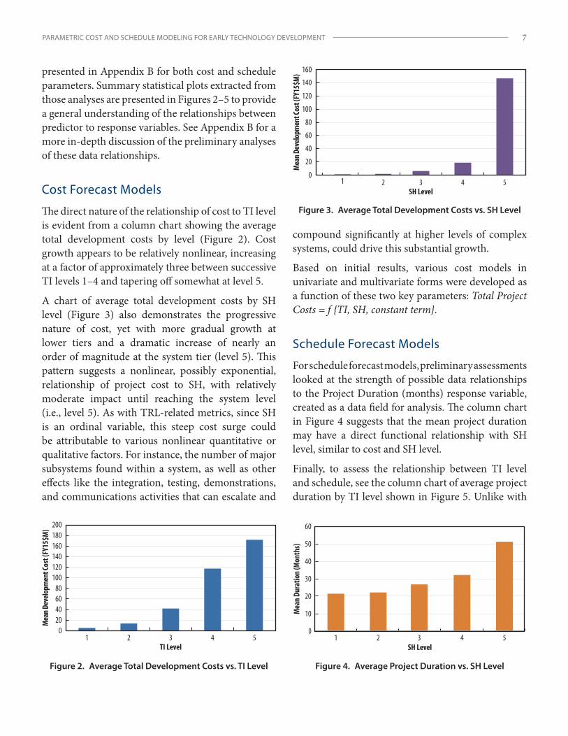
presented in Appendix B for both cost and schedule parameters. Summary statistical plots extracted from those analyses are presented in Figures 2–5 to provide a general understanding of the relationships between predictor to response variables. See Appendix B for a more in-depth discussion of the preliminary analyses of these data relationships.
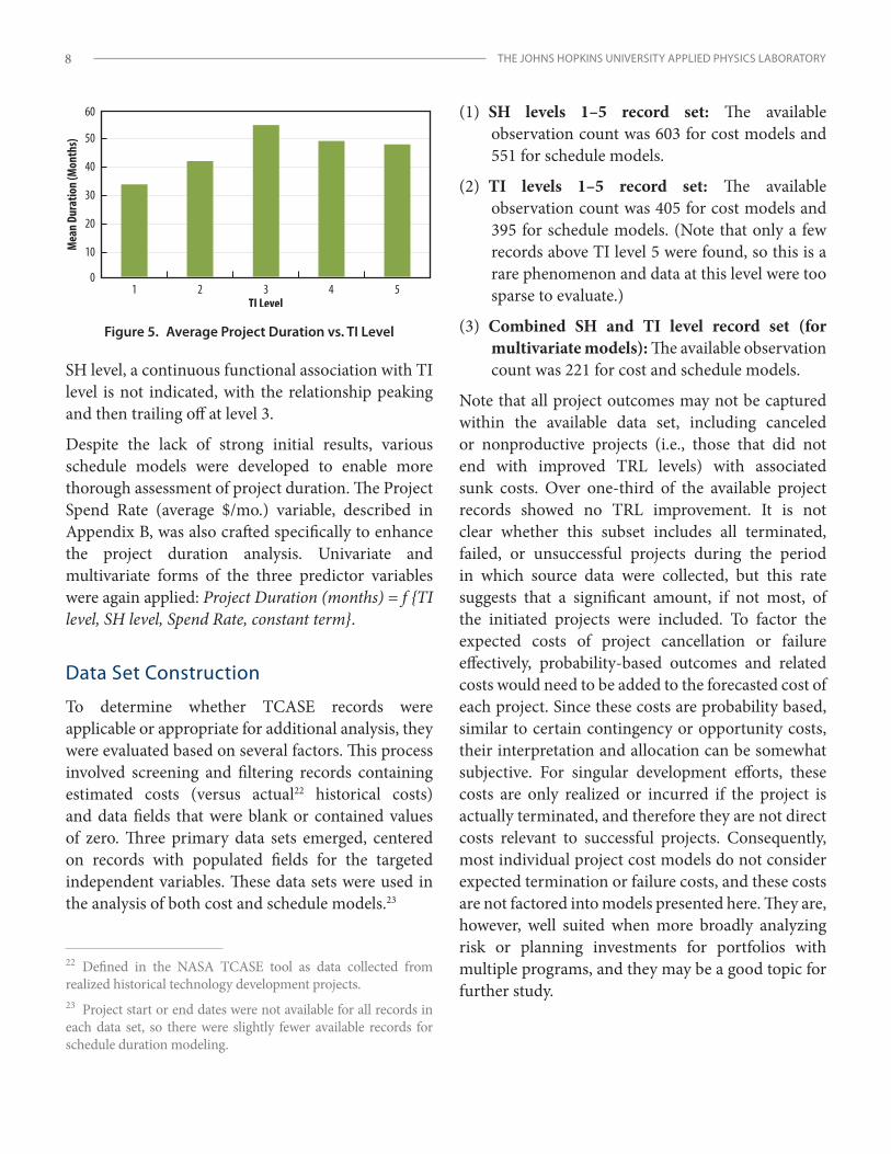
Cost Forecast Models
The direct nature of the relationship of cost to TI level is evident from a column chart showing the average total development costs by level (Figure 2). Cost growth appears to be relatively nonlinear, increasing at a factor of approximately three between successive TI levels 1–4 and tapering off somewhat at level 5.
A chart of average total development costs by SH level (Figure 3) also demonstrates the progressive nature of cost, yet with more gradual growth at lower tiers and a dramatic increase of nearly an order of magnitude at the system tier (level 5). This pattern suggests a nonlinear, possibly exponential, relationship of project cost to SH, with relatively moderate impact until reaching the system level (i.e., level 5). As with TRL-related metrics, since SH is an ordinal variable, this steep cost surge could be attributable to various nonlinear quantitative or qualitative factors. For instance, the number of major subsystems found within a system, as well as other effects like the integration, testing, demonstrations, and communications activities that can escalate and
compound significantly at higher levels of complex systems, could drive this substantial growth.
Based on initial results, various cost models in univariate and multivariate forms were developed as a function of these two key parameters: Total Project Costs = f {TI, SH, constant term}.
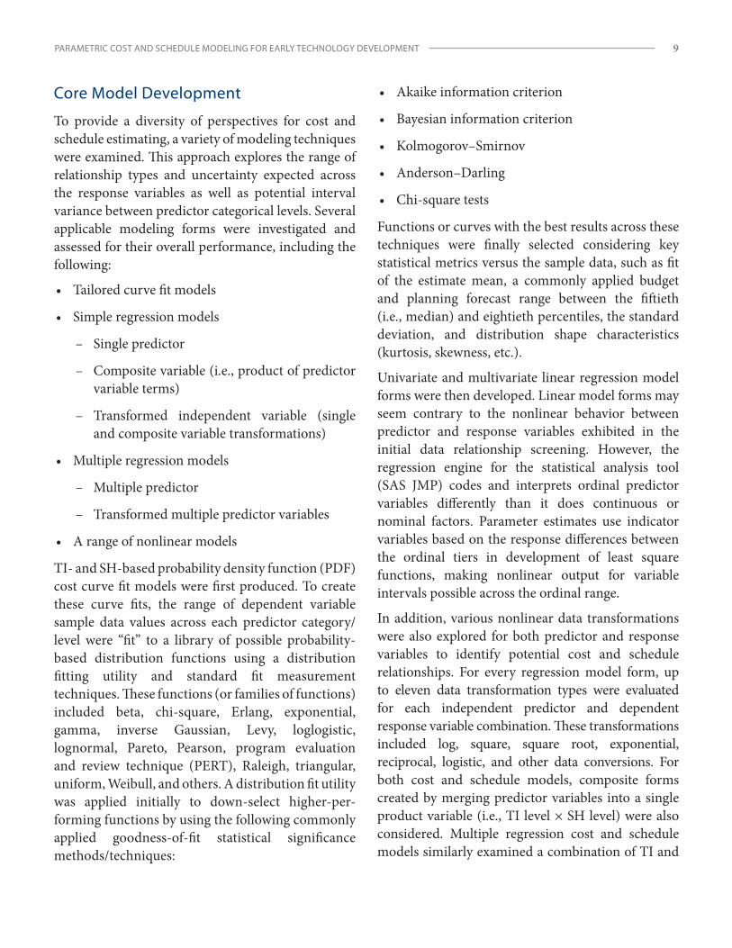
Schedule Forecast Models
For schedule forecast models, preliminary assessments looked at the strength of possible data relationships to the Project Duration (months) response variable, created as a data field for analysis. The column chart in Figure 4 suggests that the mean project duration may have a direct functional relationship with SH level, similar to cost and SH level.
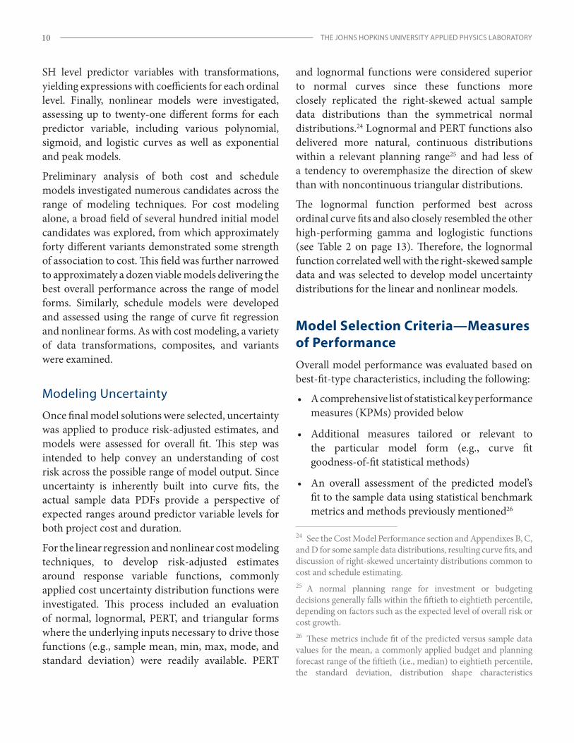
Finally, to assess the relationship between TI level and schedule, see the column chart of average project duration by TI level shown in Figure 5. Unlike with
0
20
40
60
80
100
120
140
160
Mea
n Dev
elopm
ent C
ost (
FY15
$M)
SH Level1 2 3 4 5
Figure 3. Average Total Development Costs vs. SH Level
020406080
100120140160180200
1 2 3 4 5
Mea
n Dev
elopm
ent C
ost (
FY15
$M)
TI Level
Figure 2. Average Total Development Costs vs. TI Level
0
10
20
30
40
50
60
1 2 3 4 5
Mea
n Du
ratio
n (M
onth
s)
SH Level
Figure 4. Average Project Duration vs. SH Level
THE JOHNS HOPKINS UNIVERSITY APPLIED PHYSICS LABORATORY8
SH level, a continuous functional association with TI level is not indicated, with the relationship peaking and then trailing off at level 3.
Despite the lack of strong initial results, various schedule models were developed to enable more thorough assessment of project duration. The Project Spend Rate (average $/mo.) variable, described in Appendix B, was also crafted specifically to enhance the project duration analysis. Univariate and multivariate forms of the three predictor variables were again applied: Project Duration (months) = f {TI level, SH level, Spend Rate, constant term}.
Data Set Construction
To determine whether TCASE records were applicable or appropriate for additional analysis, they were evaluated based on several factors. This process involved screening and filtering records containing estimated costs (versus actual22 historical costs) and data fields that were blank or contained values of zero. Three primary data sets emerged, centered on records with populated fields for the targeted independent variables. These data sets were used in the analysis of both cost and schedule models.23
22 Defined in the NASA TCASE tool as data collected from realized historical technology development projects.23 Project start or end dates were not available for all records in each data set, so there were slightly fewer available records for schedule duration modeling.
(1) SH levels 1–5 record set: The available observation count was 603 for cost models and 551 for schedule models.
(2) TI levels 1–5 record set: The available observation count was 405 for cost models and 395 for schedule models. (Note that only a few records above TI level 5 were found, so this is a rare phenomenon and data at this level were too sparse to evaluate.)
(3) Combined SH and TI level record set (for multivariate models): The available observation count was 221 for cost and schedule models.
Note that all project outcomes may not be captured within the available data set, including canceled or nonproductive projects (i.e., those that did not end with improved TRL levels) with associated sunk costs. Over one-third of the available project records showed no TRL improvement. It is not clear whether this subset includes all terminated, failed, or unsuccessful projects during the period in which source data were collected, but this rate suggests that a significant amount, if not most, of the initiated projects were included. To factor the expected costs of project cancellation or failure effectively, probability-based outcomes and related costs would need to be added to the forecasted cost of each project. Since these costs are probability based, similar to certain contingency or opportunity costs, their interpretation and allocation can be somewhat subjective. For singular development efforts, these costs are only realized or incurred if the project is actually terminated, and therefore they are not direct costs relevant to successful projects. Consequently, most individual project cost models do not consider expected termination or failure costs, and these costs are not factored into models presented here. They are, however, well suited when more broadly analyzing risk or planning investments for portfolios with multiple programs, and they may be a good topic for further study.
0
10
20
30
1 2 3 4 5
Mea
n Du
ratio
n (M
onth
s)
TI Level
50
40
60
Figure 5. Average Project Duration vs. TI Level
PARAMETRIC COST AND SCHEDULE MODELING FOR EARLY TECHNOLOGY DEVELOPMENT 9
Core Model Development
To provide a diversity of perspectives for cost and schedule estimating, a variety of modeling techniques were examined. This approach explores the range of relationship types and uncertainty expected across the response variables as well as potential interval variance between predictor categorical levels. Several applicable modeling forms were investigated and assessed for their overall performance, including the following:
• Tailored curve fit models
• Simple regression models
– Single predictor
– Composite variable (i.e., product of predictor variable terms)
– Transformed independent variable (single and composite variable transformations)
• Multiple regression models
– Multiple predictor
– Transformed multiple predictor variables
• A range of nonlinear models
TI- and SH-based probability density function (PDF) cost curve fit models were first produced. To create these curve fits, the range of dependent variable sample data values across each predictor category/level were “fit” to a library of possible probability- based distribution functions using a distribution fitting utility and standard fit measurement techniques. These functions (or families of functions) included beta, chi-square, Erlang, exponential, gamma, inverse Gaussian, Levy, loglogistic, lognormal, Pareto, Pearson, program evaluation and review technique (PERT), Raleigh, triangular, uniform, Weibull, and others. A distribution fit utility was applied initially to down-select higher-per-forming functions by using the following commonly applied goodness-of-fit statistical significance methods/techniques:
• Akaike information criterion
• Bayesian information criterion
• Kolmogorov–Smirnov
• Anderson–Darling
• Chi-square tests
Functions or curves with the best results across these techniques were finally selected considering key statistical metrics versus the sample data, such as fit of the estimate mean, a commonly applied budget and planning forecast range between the fiftieth (i.e., median) and eightieth percentiles, the standard deviation, and distribution shape characteristics (kurtosis, skewness, etc.).
Univariate and multivariate linear regression model forms were then developed. Linear model forms may seem contrary to the nonlinear behavior between predictor and response variables exhibited in the initial data relationship screening. However, the regression engine for the statistical analysis tool (SAS JMP) codes and interprets ordinal predictor variables differently than it does continuous or nominal factors. Parameter estimates use indicator variables based on the response differences between the ordinal tiers in development of least square functions, making nonlinear output for variable intervals possible across the ordinal range.
In addition, various nonlinear data transformations were also explored for both predictor and response variables to identify potential cost and schedule relationships. For every regression model form, up to eleven data transformation types were evaluated for each independent predictor and dependent response variable combination. These transformations included log, square, square root, exponential, reciprocal, logistic, and other data conversions. For both cost and schedule models, composite forms created by merging predictor variables into a single product variable (i.e., TI level × SH level) were also considered. Multiple regression cost and schedule models similarly examined a combination of TI and
THE JOHNS HOPKINS UNIVERSITY APPLIED PHYSICS LABORATORY10
SH level predictor variables with transformations, yielding expressions with coefficients for each ordinal level. Finally, nonlinear models were investigated, assessing up to twenty-one different forms for each predictor variable, including various polynomial, sigmoid, and logistic curves as well as exponential and peak models.
Preliminary analysis of both cost and schedule models investigated numerous candidates across the range of modeling techniques. For cost modeling alone, a broad field of several hundred initial model candidates was explored, from which approximately forty different variants demonstrated some strength of association to cost. This field was further narrowed to approximately a dozen viable models delivering the best overall performance across the range of model forms. Similarly, schedule models were developed and assessed using the range of curve fit regression and nonlinear forms. As with cost modeling, a variety of data transformations, composites, and variants were examined.
Modeling Uncertainty
Once final model solutions were selected, uncertainty was applied to produce risk-adjusted estimates, and models were assessed for overall fit. This step was intended to help convey an understanding of cost risk across the possible range of model output. Since uncertainty is inherently built into curve fits, the actual sample data PDFs provide a perspective of expected ranges around predictor variable levels for both project cost and duration.
For the linear regression and nonlinear cost modeling techniques, to develop risk-adjusted estimates around response variable functions, commonly applied cost uncertainty distribution functions were investigated. This process included an evaluation of normal, lognormal, PERT, and triangular forms where the underlying inputs necessary to drive those functions (e.g., sample mean, min, max, mode, and standard deviation) were readily available. PERT
and lognormal functions were considered superior to normal curves since these functions more closely replicated the right-skewed actual sample data distributions than the symmetrical normal distributions.24 Lognormal and PERT functions also delivered more natural, continuous distributions within a relevant planning range25 and had less of a tendency to overemphasize the direction of skew than with noncontinuous triangular distributions.
The lognormal function performed best across ordinal curve fits and also closely resembled the other high-performing gamma and loglogistic functions (see Table 2 on page 13). Therefore, the lognormal function correlated well with the right-skewed sample data and was selected to develop model uncertainty distributions for the linear and nonlinear models.
Model Selection Criteria—Measures of PerformanceOverall model performance was evaluated based on best-fit-type characteristics, including the following:
• A comprehensive list of statistical key performance measures (KPMs) provided below
• Additional measures tailored or relevant to the particular model form (e.g., curve fit goodness-of-fit statistical methods)
• An overall assessment of the predicted model’s fit to the sample data using statistical benchmark metrics and methods previously mentioned26
24 See the Cost Model Performance section and Appendixes B, C, and D for some sample data distributions, resulting curve fits, and discussion of right-skewed uncertainty distributions common to cost and schedule estimating.25 A normal planning range for investment or budgeting decisions generally falls within the fiftieth to eightieth percentile, depending on factors such as the expected level of overall risk or cost growth.26 These metrics include fit of the predicted versus sample data values for the mean, a commonly applied budget and planning forecast range of the fiftieth (i.e., median) to eightieth percentile, the standard deviation, distribution shape characteristics
PARAMETRIC COST AND SCHEDULE MODELING FOR EARLY TECHNOLOGY DEVELOPMENT 11
Statistical metrics were assessed at predictor variable ordinal levels when possible (versus at the aggregate model level) when doing so afforded greater fidelity for any measure.
Relevant KPMs applied for initial model screening include the following:
• Error variability and dispersion measures
– Coefficient of determination (R2 and adjusted R2)
– Root mean square error (RMSE)
– Coefficient of variation (CV)
• Statistical significance measures
– F-ratio
– t-stat (percent of model terms with probability greater than |t|)
• Autocorrelation measure
– Durbin–Watson test
• Data reduction measure
– Percent of original data sample set unused
See Appendix E for detailed descriptions of these statistical measures.
To assess overall performance, KPMs plus other performance measures applicable to or available for each particular model form were applied. For instance, several of the regression-related performance categories do not apply or are not available for the curve fit or nonlinear models. Curve fit models were assessed based on the five goodness-of-fit methods/techniques previously introduced (Akaike information criterion, Bayesian information crite- rion, Kolmogorov–Smirnov, Anderson–Darling, and chi-square tests), applicable KPMs (RMSE, CV, and percent of data reduction metric), and also the key data statistics described above. For nonlinear
(kurtosis, skewness, etc.), and graphical methods such as plots of residuals and model forecasts versus actual sample data.
models, available KPMs (R2, adjusted R2, RMSE, CV, and percent of data reduction) and the key data statistics were used to gauge the closeness of fit. Multicollinearity was also evaluated for multivariate model forms by applying the variance inflation factor.
Cost Model PerformanceThis section describes the performance of the various models that were evaluated, beginning with overall results and then moving to categorical model form results for curve fit cost models, simple linear regression cost models, multivariate linear regression cost models, and nonlinear cost models. Response variable output for all final cost models, including the multivariate forms, key data benchmarks, regression results, functional prediction expressions, and uncertainty functions with corresponding PDF graphs, may be available on request.
Overall Results
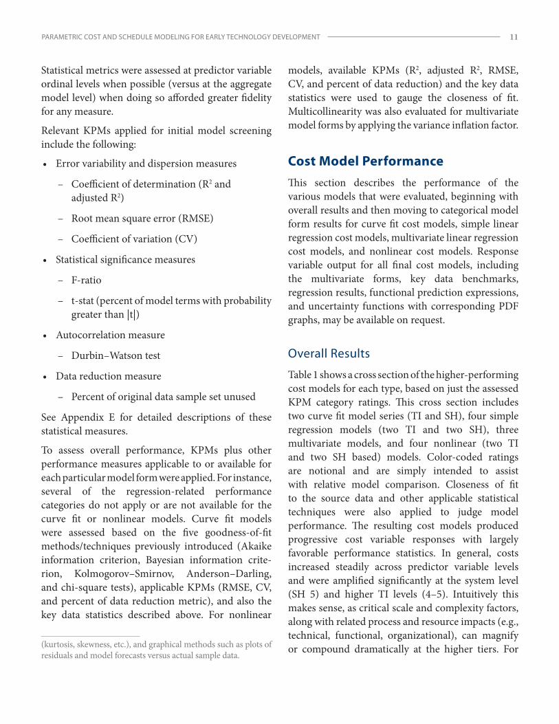
Table 1 shows a cross section of the higher-performing cost models for each type, based on just the assessed KPM category ratings. This cross section includes two curve fit model series (TI and SH), four simple regression models (two TI and two SH), three multivariate models, and four nonlinear (two TI and two SH based) models. Color-coded ratings are notional and are simply intended to assist with relative model comparison. Closeness of fit to the source data and other applicable statistical techniques were also applied to judge model performance. The resulting cost models produced progressive cost variable responses with largely favorable performance statistics. In general, costs increased steadily across predictor variable levels and were amplified significantly at the system level (SH 5) and higher TI levels (4–5). Intuitively this makes sense, as critical scale and complexity factors, along with related process and resource impacts (e.g., technical, functional, organizational), can magnify or compound dramatically at the higher tiers. For
THE JOHNS HOPKINS UNIVERSITY APPLIED PHYSICS LABORATORY12
system-level (SH 5) technology developments, it appears essential to apply SH level variable models but much less important below level 5, based on relationship screening (Appendix B) and the detailed results in the models shown in Table 1.
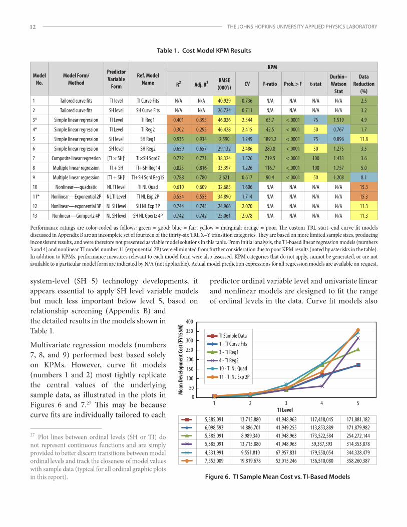
Multivariate regression models (numbers 7, 8, and 9) performed best based solely on KPMs. However, curve fit models (numbers 1 and 2) most tightly replicate the central values of the underlying sample data, as illustrated in the plots in Figures 6 and 7.27 This may be because curve fits are individually tailored to each
27 Plot lines between ordinal levels (SH or TI) do not represent continuous functions and are simply provided to better discern transitions between model ordinal levels and track the closeness of model values with sample data (typical for all ordinal graphic plots in this report). Figure 6. TI Sample Mean Cost vs. TI-Based Models
5,385,0916,098,5935,385,0915,385,0914,331,9917,552,009
13,715,88014,886,7018,989,340
13,715,8809,551,810
19,819,678
41,948,96341,949,25541,948,96341,948,96367,957,83152,015,246
117,418,045113,853,889173,522,58459,337,393
179,550,054136,510,080
171,881,182171,879,982254,272,144314,353,878344,328,479358,260,387
1 2 3 4 50
50
100
150
200
250
300
350
400
Mea
n De
velo
pmen
t Cos
t (FY
15$M
)
TI Level
TI Sample Data1 - TI Curve Fits3 - TI Reg14 - TI Reg210 - TI NL Quad11 - TI NL Exp 2P
predictor ordinal variable level and univariate linear and nonlinear models are designed to fit the range of ordinal levels in the data. Curve fit models also
Table 1. Cost Model KPM Results
Model No.
Model Form/ Method
Predictor Variable
Form
Ref. Model Name
KPM
R2 Adj. R2 RMSE (000’s)
CV F-ratio Prob. > F t-statDurbin–Watson
Stat
Data Reduction
(%)
1 Tailored curve fits TI level TI Curve Fits N/A N/A 40,929 0.736 N/A N/A N/A N/A 2.5
2 Tailored curve fits SH level SH Curve Fits N/A N/A 26,724 0.711 N/A N/A N/A N/A 3.2
3* Simple linear regression TI Level TI Reg1 0.401 0.395 46,026 2.344 63.7 <.0001 75 1.519 4.9
4* Simple linear regression TI Level TI Reg2 0.302 0.295 46,428 2.415 42.5 <.0001 50 0.767 1.7
5 Simple linear regression SH level SH Reg1 0.935 0.934 2,590 1.249 1893.2 <.0001 75 0.896 11.8
6 Simple linear regression SH level SH Reg2 0.659 0.657 29,132 2.486 280.8 <.0001 50 1.275 3.5
7 Composite linear regression [TI × SH]2 TI×SH Sqrd7 0.772 0.771 38,324 1.526 719.5 <.0001 100 1.433 3.6
8 Multiple linear regression TI + SH TI+SH Reg14 0.823 0.816 33,397 1.226 116.7 <.0001 100 1.757 5.0
9 Multiple linear regression [TI + SH]2 TI+SH Sqrd Reg15 0.788 0.780 2,621 0.617 90.4 <.0001 50 1.208 8.1
10 Nonlinear—quadratic NL TI level TI NL Quad 0.610 0.609 32,685 1.606 N/A N/A N/A N/A 15.3
11* Nonlinear—Exponential 2P NL TI Level TI NL Exp 2P 0.554 0.553 34,890 1.714 N/A N/A N/A N/A 15.3
12 Nonlinear—exponential 3P NL SH level SH NL Exp 3P 0.744 0.743 24,966 2.070 N/A N/A N/A N/A 11.3
13 Nonlinear—Gompertz 4P NL SH level SH NL Gpertz 4P 0.742 0.742 25,061 2.078 N/A N/A N/A N/A 11.3
Performance ratings are color-coded as follows: green = good; blue = fair; yellow = marginal; orange = poor. The custom TRL start–end curve fit models discussed in Appendix B are an incomplete set of fourteen of the thirty-six TRL X–Y transition categories. They are based on more limited sample sizes, producing inconsistent results, and were therefore not presented as viable model solutions in this table. From initial analysis, the TI-based linear regression models (numbers 3 and 4) and nonlinear TI model number 11 (exponential 2P) were eliminated from further consideration due to poor KPM results (noted by asterisks in the table). In addition to KPMs, performance measures relevant to each model form were also assessed. KPM categories that do not apply, cannot be generated, or are not available to a particular model form are indicated by N/A (not applicable). Actual model prediction expressions for all regression models are available on request.
PARAMETRIC COST AND SCHEDULE MODELING FOR EARLY TECHNOLOGY DEVELOPMENT 13
essentially neutralize the issue of interval ordinal scale variability, since each level is discretely modeled to align more directly with uncertainty distributions of the actual sample data. Linear regression and nonlinear models generally employ more of a one-function-fits-all approach. However, statistical regression engines also mitigate the concern of interval ordinal scale variability by the method with which they handle predictor ordinal
values, as discussed in the Core Model Development section.
Curve Fit Cost Models
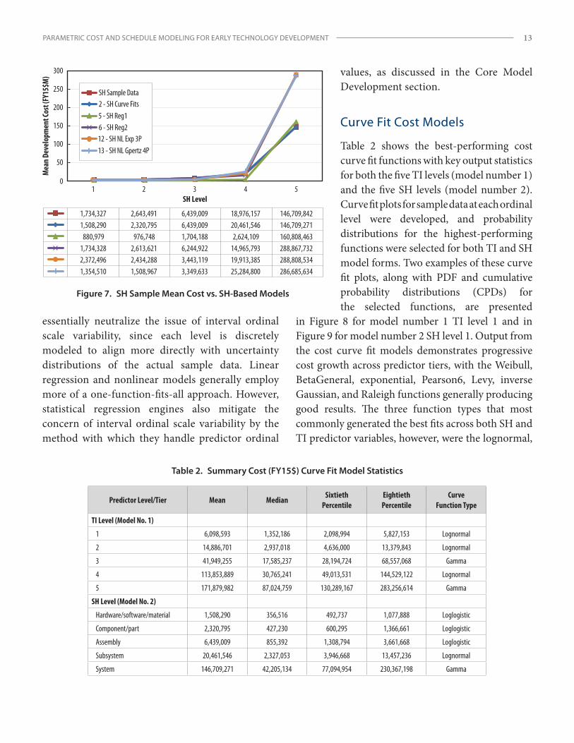
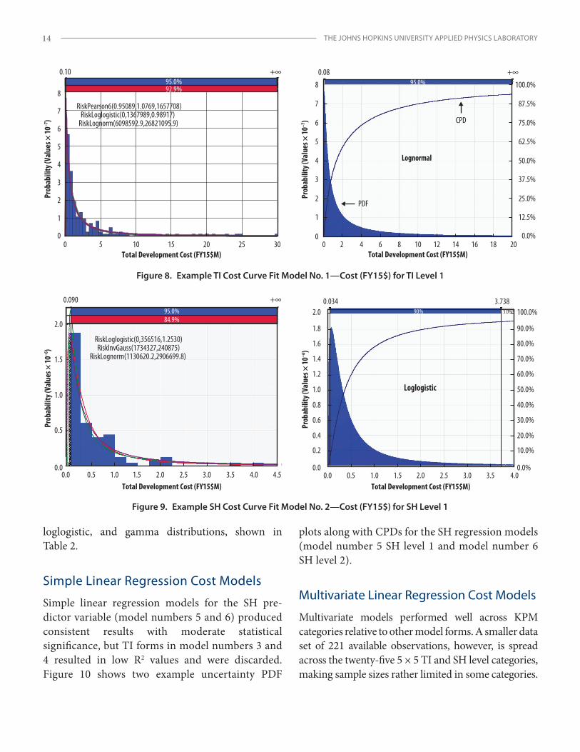
Table 2 shows the best-performing cost curve fit functions with key output statistics for both the five TI levels (model number 1) and the five SH levels (model number 2). Curve fit plots for sample data at each ordinal level were developed, and probability distributions for the highest-performing functions were selected for both TI and SH model forms. Two examples of these curve fit plots, along with PDF and cumulative probability distributions (CPDs) for the selected functions, are presented
in Figure 8 for model number 1 TI level 1 and in Figure 9 for model number 2 SH level 1. Output from the cost curve fit models demonstrates progressive cost growth across predictor tiers, with the Weibull, BetaGeneral, exponential, Pearson6, Levy, inverse Gaussian, and Raleigh functions generally producing good results. The three function types that most commonly generated the best fits across both SH and TI predictor variables, however, were the lognormal,
Figure 7. SH Sample Mean Cost vs. SH-Based Models
1,734,3271,508,290
880,9791,734,3282,372,4961,354,510
2,643,4912,320,795
976,7482,613,6212,434,2881,508,967
6,439,0096,439,0091,704,1886,244,9223,443,1193,349,633
18,976,15720,461,5462,624,109
14,965,79319,913,38525,284,800
146,709,842146,709,271160,808,463288,867,732288,808,534286,685,634
0
50
100
150
200
250
300
1 2 3 4 5
Mea
n De
velo
pmen
t Cos
t (FY
15$M
)
SH Level
SH Sample Data2 - SH Curve Fits5 - SH Reg16 - SH Reg212 - SH NL Exp 3P13 - SH NL Gpertz 4P
Table 2. Summary Cost (FY15$) Curve Fit Model Statistics
Predictor Level/Tier Mean MedianSixtieth
PercentileEightieth Percentile
Curve Function Type
TI Level (Model No. 1)
1 6,098,593 1,352,186 2,098,994 5,827,153 Lognormal
2 14,886,701 2,937,018 4,636,000 13,379,843 Lognormal
3 41,949,255 17,585,237 28,194,724 68,557,068 Gamma
4 113,853,889 30,765,241 49,013,531 144,529,122 Lognormal
5 171,879,982 87,024,759 130,289,167 283,256,614 Gamma
SH Level (Model No. 2)
Hardware/software/material 1,508,290 356,516 492,737 1,077,888 Loglogistic
Component/part 2,320,795 427,230 600,295 1,366,661 Loglogistic
Assembly 6,439,009 855,392 1,308,794 3,661,668 Loglogistic
Subsystem 20,461,546 2,327,053 3,946,668 13,457,236 Lognormal
System 146,709,271 42,205,134 77,094,954 230,367,198 Gamma
THE JOHNS HOPKINS UNIVERSITY APPLIED PHYSICS LABORATORY14
loglogistic, and gamma distributions, shown in Table 2.
Simple Linear Regression Cost Models
Simple linear regression models for the SH pre- dictor variable (model numbers 5 and 6) produced consistent results with moderate statistical significance, but TI forms in model numbers 3 and 4 resulted in low R2 values and were discarded. Figure 10 shows two example uncertainty PDF
plots along with CPDs for the SH regression models (model number 5 SH level 1 and model number 6 SH level 2).
Multivariate Linear Regression Cost Models
Multivariate models performed well across KPM categories relative to other model forms. A smaller data set of 221 available observations, however, is spread across the twenty-five 5 × 5 TI and SH level categories, making sample sizes rather limited in some categories.
Total Development Cost (FY15$M)
0.090
2.0
1.5
1.0
0.5
0.0
+∞
84.9%
1.0 1.5 2.0 2.5 3.0 3.5 4.0 4.50.50.0
RiskLoglogistic(0,356516,1.2530)RiskInvGauss(1734327,240875)
RiskLognorm(1130620.2,2906699.8)
95.0%
Prob
abili
ty (V
alue
s × 10
–6)
0.4
0.6
0.8
1.0
1.2
1.4
1.6
1.8
2.0
0.2
0.0 0.0%
20.0%
10.0%
30.0%
40.0%
50.0%
60.0%
70.0%
80.0%
90.0%
100.0%
Loglogistic
5.0%90%0.034 3.738
Total Development Cost (FY15$M)0.50.0 1.51.0 2.52.0 3.0 3.5 4.0
Prob
abili
ty (V
alue
s × 10
–6)
Figure 9. Example SH Cost Curve Fit Model No. 2—Cost (FY15$) for SH Level 1
Total Development Cost (FY15$M)
0.10 +∞
0 5 10 15 20 25 30
8
7
6
5
4
3
2
1
0
92.9%95.0%
RiskPearson6(0.95089,1.0769,1657708)RiskLoglogistic(0,1367989,0.98917)
RiskLognorm(6098592.9,26821095.9)
Prob
abili
ty (V
alue
s × 10
–7)
0.088
7
6
5
4
3
2
1
0
Total Development Cost (FY15$M)0 42 86 1210 14 16 18 20
0.0%
12.5%
25.0%
37.5%
50.0%
62.5%
75.0%
87.5%
100.0%+∞
95.0%
Lognormal
Prob
abili
ty (V
alue
s × 10
–7)
CPD
Figure 8. Example TI Cost Curve Fit Model No. 1—Cost (FY15$) for TI Level 1
PARAMETRIC COST AND SCHEDULE MODELING FOR EARLY TECHNOLOGY DEVELOPMENT 15
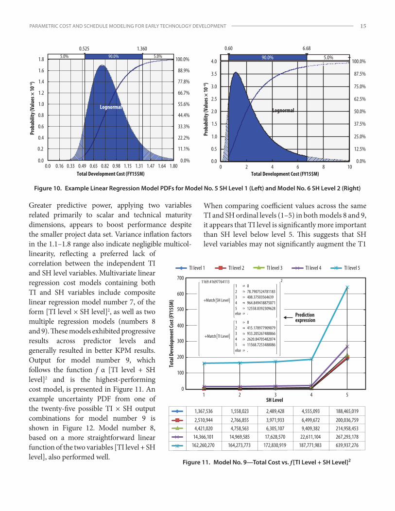
Greater predictive power, applying two variables related primarily to scalar and technical maturity dimensions, appears to boost performance despite the smaller project data set. Variance inflation factors in the 1.1–1.8 range also indicate negligible multicol-linearity, reflecting a preferred lack of correlation between the independent TI and SH level variables. Multivariate linear regression cost models containing both TI and SH variables include composite linear regression model number 7, of the form [TI level × SH level]2, as well as two multiple regression models (numbers 8 and 9). These models exhibited progressive results across predictor levels and generally resulted in better KPM results. Output for model number 9, which follows the function f α [TI level + SH level]2 and is the highest-performing cost model, is presented in Figure 11. An example uncertainty PDF from one of the twenty-five possible TI × SH output combinations for model number 9 is shown in Figure 12. Model number 8, based on a more straightforward linear function of the two variables [TI level + SH level], also performed well.
When comparing coefficient values across the same TI and SH ordinal levels (1–5) in both models 8 and 9, it appears that TI level is significantly more important than SH level below level 5. This suggests that SH level variables may not significantly augment the T1
Total Development Cost (FY15$M)
0.525 1.360
0.0 0.16 0.33 0.49 0.65 0.82 0.98 1.15 1.31 1.47 1.64 1.800.0
0.2
0.4
0.6
0.8
1.0
1.2
1.4
1.6
1.8
Prob
abili
ty (V
alue
s × 10
–6)
0.0%
11.1%
22.2%
33.3%
44.4%
55.6%
66.7%
77.8%
88.9%
100.0%
90.0%5.0% 90.0% 5.0%
Lognormal
Total Development Cost (FY15$M)
6.680.60
0 2 4 6 8 100.0
0.5
1.0
1.5
2.0
2.5
3.0
3.5
4.0
12.5%
25.0%
37.5%
50.0%
62.5%
75.0%
87.5%
100.0%
0.0%
90.0% 5.0%
Lognormal
Prob
abili
ty (V
alue
s × 10
–6)
Figure 10. Example Linear Regression Model PDFs for Model No. 5 SH Level 1 (Left) and Model No. 6 SH Level 2 (Right)
1,367,536 1,558,023 2,489,428 4,555,093 188,465,019
2,510,944 2,766,855 3,971,933 6,499,672 200,036,7594,421,020 4,758,563 6,305,107 9,409,382 214,958,453
14,366,101 14,969,585 17,628,570 22,611,104 267,293,178162,260,270 164,273,773 172,830,919 187,771,983 639,937,276
1 2 3 4 5
100
0
200
300
400
500
600
700
Tota
l Dev
elop
men
t Cos
t (FY
15$M
)
SH Level
Predictionexpression
+Match TI Level
else
12345
078.7907524781183408.37503564639964.84941887507112558.8392309628.
21169.41697764113
+Match SH Level
else
0415.178977909079933.2052674888662620.8470548207411568.7253488086.
12345
TI level 1 TI level 2 TI level 3 TI level 4 TI level 5
Figure 11. Model No. 9—Total Cost vs. f [TI Level + SH Level]2
THE JOHNS HOPKINS UNIVERSITY APPLIED PHYSICS LABORATORY16
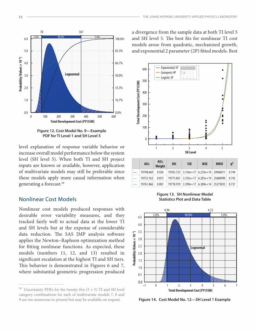
level explanation of response variable behavior or increase overall model performance below the system level (SH level 5). When both TI and SH project inputs are known or available, however, application of multivariate models may still be preferable since these models apply more causal information when generating a forecast.28
Nonlinear Cost Models
Nonlinear cost models produced responses with desirable error variability measures, and they tracked fairly well to actual data at the lower TI and SH levels but at the expense of considerable data reduction. The SAS JMP analysis software applies the Newton–Raphson optimization method for fitting nonlinear functions. As expected, these models (numbers 11, 12, and 13) resulted in significant escalation at the highest TI and SH tiers. This behavior is demonstrated in Figures 6 and 7, where substantial geometric progression produced
28 Uncertainty PDFs for the twenty-five (5 × 5) TI and SH level category combinations for each of multivariate models 7, 8 and 9 are too numerous to present but may be available on request.
a divergence from the sample data at both TI level 5 and SH level 5. The best fits for nonlinear TI cost models arose from quadratic, mechanized growth, and exponential 2 parameter (2P) fitted models. Best
0.0
0.94 4.72
–1 0 1 2 3 4 5 6 7Total Development Cost (FY15$M)
0.5
1.0
1.5
2.0
2.5
3.0
3.5
4.0
5.0% 90.0% 5.0%4.5
Lognormal
Prob
abili
ty (V
alue
s × 10
–7)
Figure 14. Cost Model No. 12—SH Level 1 Example
1.0
2.0
3.0
4.0
5.0
6.0
0.0 0.0%
16.7%
33.3%
50.0%
66.7%
83.3%
100.0%
Total Development Cost (FY15$M)1000 200 300 400 500 600
Prob
abili
ty (V
alue
s × 10
–9)
78 3675.0% 5.0%90.0%
Lognormal
Figure 12. Cost Model No. 9—Example PDF for TI Level 1 and SH Level 5
Figure 13. SH Nonlinear Model Statistics Plot and Data Table
0
100
200
300
400
500
600
1 2 3 4 5
Tota
l Dev
elop
men
t Cos
t (FY
15$M
)
SH Level
Exponential 3PGompertz 4PLogistic 3P
. . .6 .8
AICcAICc
WeightBIC SSE MSE RMSE R2
— 19748.669 0.926 19765.723 3.316e+17 6.233e+14 24966011 0.744
— 19753.763 0.073 19775.061 3.335e+17 6.281e+14 25060990 0.742
— 19761.866 0.001 19778.919 3.399e+17 6.389e+14 25275833 0.737
PARAMETRIC COST AND SCHEDULE MODELING FOR EARLY TECHNOLOGY DEVELOPMENT 17
fits for the nonlinear SH cost models were generated by exponential 3 parameter (3P) and Gompertz 4 parameter (4P) functional forms. A plot of SH nonlinear models is presented in Figure 13, and an example uncertainty PDF graph for SH level 1 of SH model number 12 is provided in Figure 14. TI nonlinear model number 11 was eliminated due to poor KPM results.
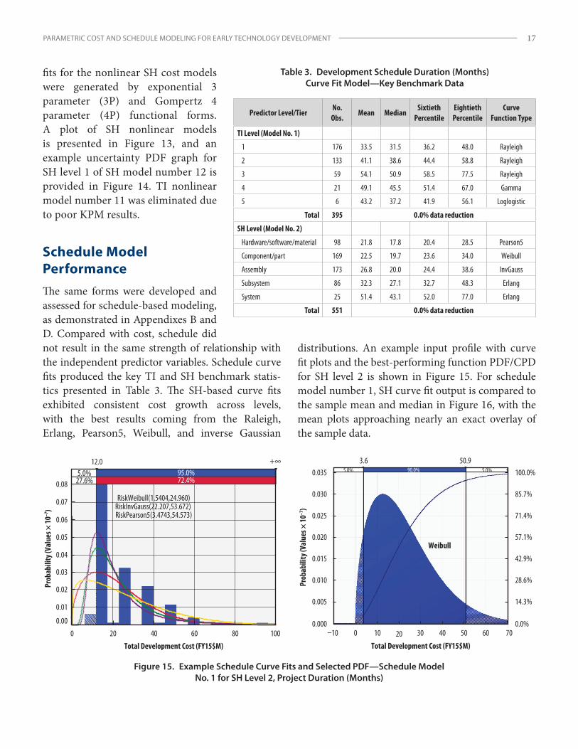
Schedule Model PerformanceThe same forms were developed and assessed for schedule-based modeling, as demonstrated in Appendixes B and D. Compared with cost, schedule did not result in the same strength of relationship with the independent predictor variables. Schedule curve fits produced the key TI and SH benchmark statis- tics presented in Table 3. The SH-based curve fits exhibited consistent cost growth across levels, with the best results coming from the Raleigh, Erlang, Pearson5, Weibull, and inverse Gaussian
distributions. An example input profile with curve fit plots and the best-performing function PDF/CPD for SH level 2 is shown in Figure 15. For schedule model number 1, SH curve fit output is compared to the sample mean and median in Figure 16, with the mean plots approaching nearly an exact overlay of the sample data.
Table 3. Development Schedule Duration (Months) Curve Fit Model—Key Benchmark Data
Predictor Level/TierNo.
Obs.Mean Median
SixtiethPercentile
Eightieth Percen tile
Curve Function Type
TI Level (Model No. 1)
1 176 33.5 31.5 36.2 48.0 Rayleigh
2 133 41.1 38.6 44.4 58.8 Rayleigh
3 59 54.1 50.9 58.5 77.5 Rayleigh
4 21 49.1 45.5 51.4 67.0 Gamma
5 6 43.2 37.2 41.9 56.1 Loglogistic
Total 395 0.0% data reduction
SH Level (Model No. 2)
Hardware/software/material 98 21.8 17.8 20.4 28.5 Pearson5
Component/part 169 22.5 19.7 23.6 34.0 Weibull
Assembly 173 26.8 20.0 24.4 38.6 InvGauss
Subsystem 86 32.3 27.1 32.7 48.3 Erlang
System 25 51.4 43.1 52.0 77.0 Erlang
Total 551 0.0% data reduction
5.0% 95.0%27.6% 72.4%
12.0 +∞
6040200 80 1000.00
0.01
0.02
0.03
0.04
0.05
0.06
0.07
0.08
RiskWeibull(1.5404,24.960)RiskInvGauss(22.207,53.672) RiskPearson5(3.4743,54.573)
Total Development Cost (FY15$M)
Prob
abili
ty (V
alue
s × 10
–7)
0.035
0.030
0.025
0.020
0.015
0.010
0.005
0.000
3.6 50.9
0 10 20 30 40 50 60 70–100.0%
14.3%
28.6%
42.9%
57.1%
71.4%
85.7%
100.0%
Total Development Cost (FY15$M)
Weibull
5.0%5.0% 90.0%
Prob
abili
ty (V
alue
s × 10
–7)
Figure 15. Example Schedule Curve Fits and Selected PDF—Schedule Model No. 1 for SH Level 2, Project Duration (Months)
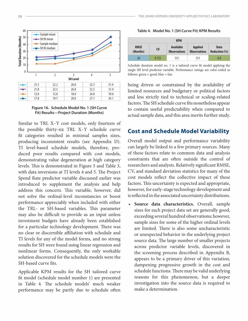
THE JOHNS HOPKINS UNIVERSITY APPLIED PHYSICS LABORATORY18
being driven or constrained by the availability of limited resources and budgetary or political factors and less strictly tied to technical or scaling-related factors. The SH schedule curve fits nonetheless appear to contain useful predictability when compared to actual sample data, and this area merits further study.
Cost and Schedule Model VariabilityOverall model output and performance variability can largely be linked to a few primary sources. Many of these factors relate to common data and analysis constraints that are often outside the control of researchers and analysts. Relatively significant RMSE, CV, and standard deviation statistics for many of the cost models reflect the collective impact of these factors. This uncertainty is expected and appropriate, however, for early-stage technology development and is reflected in the associated uncertainty distributions.
• Source data characteristics. Overall, sample sizes for each project data set are generally good, exceeding several hundred observations; however, sample sizes for some of the higher ordinal levels are limited. There is also some uncharacteristic or unexpected behavior in the underlying project source data. The large number of smaller projects across predictor variable levels, discovered in the screening process described in Appendix B, appears to be a primary driver of this variation, dampening progressive growth in the cost and schedule functions. There may be valid underlying reasons for this phenomenon, but a deeper investigation into the source data is required to make a determination.
Table 4. Model No. 1 (SH Curve Fit) KPM Results
KPM
RMSE (Months)
CVAvailable
ObservationsApplied
ObservationsData
Reduction (%)
20 0.755 551 551 0.0
Schedule duration model no. 1 is a tailored curve fit model applying the single SH level predictor variable. Performance ratings are color-coded as follows: green = good; blue = fair.
Similar to TRL X–Y cost models, only fourteen of the possible thirty-six TRL X–Y schedule curve fit categories resulted in minimal samples sizes, producing inconsistent results (see Appendix D). TI level-based schedule models, therefore, pro- duced poor results compared with cost models, demonstrating value degeneration at high category levels. This is demonstrated in Figure 5 and Table 3, with data inversions at TI levels 4 and 5. The Project Spend Rate predictor variable discussed earlier was introduced to supplement the analysis and help address this concern. This variable, however, did not solve the ordinal-level inconstancies or boost performance appreciably when included with either the TRL- or SH-based variables. This parameter may also be difficult to provide as an input unless investment budgets have already been established for a particular technology development. There was no clear or discernible affiliation with schedule and TI levels for any of the model forms, and no strong results for SH were found using linear regression and nonlinear forms. Consequently, the only workable solution discovered for the schedule models were the SH-based curve fits.
Applicable KPM results for the SH tailored curve fit model (schedule model number 1) are presented in Table 4. The schedule models’ much weaker performance may be partly due to schedule often
Figure 16. Schedule Model No. 1 (SH Curve Fit) Results —Project Duration (Months)
21.5 22.2 26.8 32.3 51.421.8 22.5 26.8 32.3 51.412.0 12.0 18.0 24.0 39.017.8 19.7 20.0 27.1 43.1
1 2 3 4 50
10
20
30
40
50
60
Tota
l Dur
atio
n (M
onth
s)
SH Level
Sample meanSH �t meanSample medianSH �t median
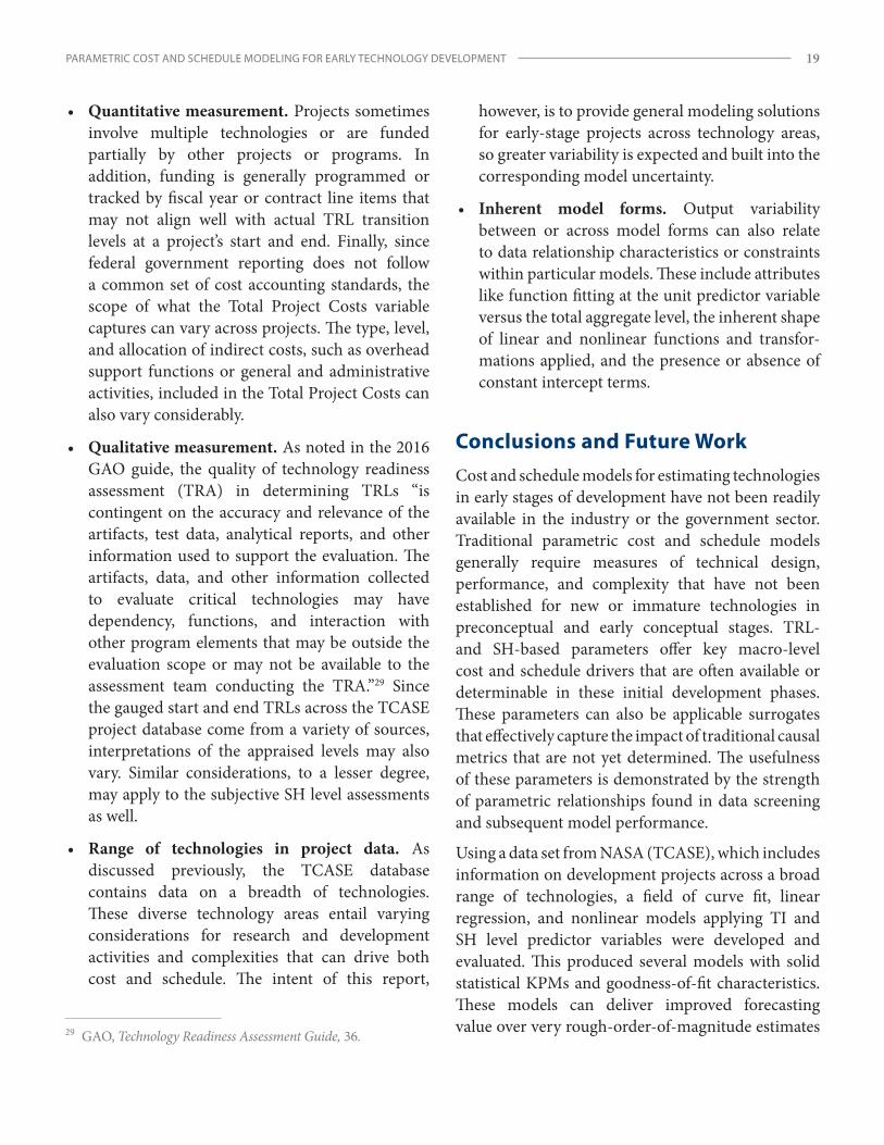
PARAMETRIC COST AND SCHEDULE MODELING FOR EARLY TECHNOLOGY DEVELOPMENT 19
• Quantitative measurement. Projects sometimes involve multiple technologies or are funded partially by other projects or programs. In addition, funding is generally programmed or tracked by fiscal year or contract line items that may not align well with actual TRL transition levels at a project’s start and end. Finally, since federal government reporting does not follow a common set of cost accounting standards, the scope of what the Total Project Costs variable captures can vary across projects. The type, level, and allocation of indirect costs, such as overhead support functions or general and administrative activities, included in the Total Project Costs can also vary considerably.
• Qualitative measurement. As noted in the 2016 GAO guide, the quality of technology readiness assessment (TRA) in determining TRLs “is contingent on the accuracy and relevance of the artifacts, test data, analytical reports, and other information used to support the evaluation. The artifacts, data, and other information collected to evaluate critical technologies may have dependency, functions, and interaction with other program elements that may be outside the evaluation scope or may not be available to the assessment team conducting the TRA.”29 Since the gauged start and end TRLs across the TCASE project database come from a variety of sources, interpretations of the appraised levels may also vary. Similar considerations, to a lesser degree, may apply to the subjective SH level assessments as well.
• Range of technologies in project data. As discussed previously, the TCASE database contains data on a breadth of technologies. These diverse technology areas entail varying considerations for research and development activities and complexities that can drive both cost and schedule. The intent of this report,
29 GAO, Technology Readiness Assessment Guide, 36.
however, is to provide general modeling solutions for early-stage projects across technology areas, so greater variability is expected and built into the corresponding model uncertainty.
• Inherent model forms. Output variability between or across model forms can also relate to data relationship characteristics or constraints within particular models. These include attributes like function fitting at the unit predictor variable versus the total aggregate level, the inherent shape of linear and nonlinear functions and transfor-mations applied, and the presence or absence of constant intercept terms.
Conclusions and Future WorkCost and schedule models for estimating technologies in early stages of development have not been readily available in the industry or the government sector. Traditional parametric cost and schedule models generally require measures of technical design, performance, and complexity that have not been established for new or immature technologies in preconceptual and early conceptual stages. TRL- and SH-based parameters offer key macro-level cost and schedule drivers that are often available or determinable in these initial development phases. These parameters can also be applicable surrogates that effectively capture the impact of traditional causal metrics that are not yet determined. The usefulness of these parameters is demonstrated by the strength of parametric relationships found in data screening and subsequent model performance.
Using a data set from NASA (TCASE), which includes information on development projects across a broad range of technologies, a field of curve fit, linear regression, and nonlinear models applying TI and SH level predictor variables were developed and evaluated. This produced several models with solid statistical KPMs and goodness-of-fit characteristics. These models can deliver improved forecasting value over very rough-order-of-magnitude estimates
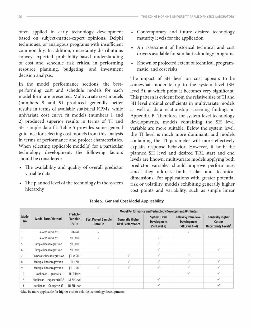
THE JOHNS HOPKINS UNIVERSITY APPLIED PHYSICS LABORATORY20
often applied in early technology development based on subject-matter-expert opinions, Delphi techniques, or analogous programs with insufficient commonality. In addition, uncertainty distributions convey expected probability-based understanding of cost and schedule risk critical in performing resource planning, budgeting, and investment decision analysis.
In the model performance sections, the best- performing cost and schedule models for each model form are presented. Multivariate cost models (numbers 8 and 9) produced generally better results in terms of available statistical KPMs, while univariate cost curve fit models (numbers 1 and 2) produced superior results in terms of TI and SH sample data fit. Table 5 provides some general guidance for selecting cost models from this analysis in terms of performance and project characteristics. When selecting applicable model(s) for a particular technology development, the following factors should be considered:
• The availability and quality of overall predictor variable data
• The planned level of the technology in the system hierarchy
• Contemporary and future desired technology maturity levels for the application
• An assessment of historical technical and cost drivers available for similar technology programs
• Known or projected extent of technical, program-matic, and cost risks
The impact of SH level on cost appears to be somewhat moderate up to the system level (SH level 5), at which point it becomes very significant. This pattern is evident from the relative size of TI and SH level ordinal coefficients in multivariate models as well as data relationship screening findings in Appendix B. Therefore, for system-level technology developments, models containing the SH level variable are more suitable. Below the system level, the TI level is much more dominant, and models containing the TI parameter will more effectively explain response behavior. However, if both the planned SH level and desired TRL start and end levels are known, multivariate models applying both predictor variables should improve performance, since they address both scalar and technical dimensions. For applications with greater potential risk or volatility, models exhibiting generally higher cost points and variability, such as simple linear
Table 5. General Cost Model Applicability
Model No.
Model Form/MethodPredictor Variable
Form
Model Performance and Technology Development Attributes
Best Project Sample Data Fit
Generally Higher KPM Performance
System-Level Development
(SH Level 5)
Below System-Level Development (SH Level 1–4)
Generally Higher Cost or
Uncertainty Levelsa
1 Tailored curve fits TI Level
2 Tailored curve fits SH Level
5 Simple linear regression SH Level
6 Simple linear regression SH Level
7 Composite linear regression [TI × SH]2
8 Multiple linear regression TI + SH
9 Multiple linear regression [TI + SH]2
10 Nonlinear—quadratic NL TI level
12 Nonlinear—exponential 3P NL SH level
13 Nonlinear—Gompertz 4P NL SH Level a May be more applicable for higher-risk or volatile technology developments.
PARAMETRIC COST AND SCHEDULE MODELING FOR EARLY TECHNOLOGY DEVELOPMENT 21
regression or nonlinear cost models, may be more applicable, especially at the higher ordinal tiers. Schedule modeling produced more limited results but produced reasonable SH-based duration curve fits and deserves further study.
If the TCASE database or other data sources are expanded to include additional project data for key response and predictor variables like RD3, technology area, and capability demonstrations, that could improve model robustness and accuracy and reduce output variability. Beyond RD3, technology area, and capability demonstrations, additional macro cost and schedule parameters that may enhance early-stage technology development forecasting include the following:
• Advanced degree of difficulty (AD2)
• System readiness level (SRL)
• Integration readiness level (IRL)
• Implementation readiness level (ImpRL)
• Manufacturing readiness level (MRL)
• System level or scalar, performance, or complexity factors applicable to a broad range of technologies
Leveraging these types of metrics to better integrate cost and schedule modeling with technology road mapping, early systems engineering, and conceptual design efforts should help decision makers with more consistent development estimates. More accurate estimates in turn effect better investment and design decisions with greater cost impact early in the project life cycle.

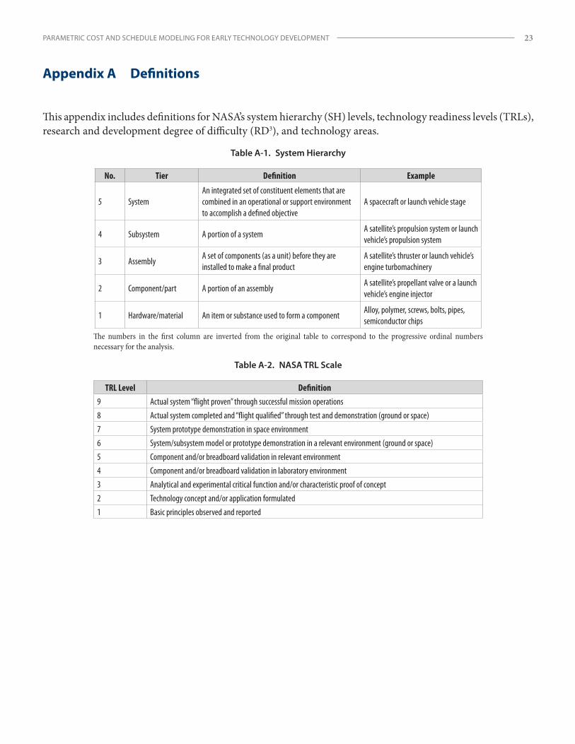
PARAMETRIC COST AND SCHEDULE MODELING FOR EARLY TECHNOLOGY DEVELOPMENT 23
Appendix A Definitions
This appendix includes definitions for NASA’s system hierarchy (SH) levels, technology readiness levels (TRLs), research and development degree of difficulty (RD3), and technology areas.
Table A-1. System Hierarchy
No. Tier Definition Example
5 SystemAn integrated set of constituent elements that are combined in an operational or support environment to accomplish a defined objective
A spacecraft or launch vehicle stage
4 Subsystem A portion of a systemA satellite’s propulsion system or launch vehicle’s propulsion system
3 AssemblyA set of components (as a unit) before they are installed to make a final product
A satellite’s thruster or launch vehicle’s engine turbomachinery
2 Component/part A portion of an assemblyA satellite’s propellant valve or a launch vehicle’s engine injector
1 Hardware/material An item or substance used to form a componentAlloy, polymer, screws, bolts, pipes, semiconductor chips
The numbers in the first column are inverted from the original table to correspond to the progressive ordinal numbers necessary for the analysis.
Table A-2. NASA TRL Scale
TRL Level Definition9 Actual system “flight proven” through successful mission operations8 Actual system completed and “flight qualified” through test and demonstration (ground or space)7 System prototype demonstration in space environment6 System/subsystem model or prototype demonstration in a relevant environment (ground or space)5 Component and/or breadboard validation in relevant environment4 Component and/or breadboard validation in laboratory environment3 Analytical and experimental critical function and/or characteristic proof of concept2 Technology concept and/or application formulated1 Basic principles observed and reported
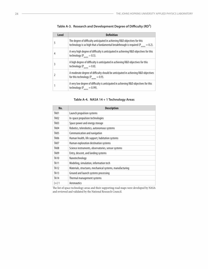
THE JOHNS HOPKINS UNIVERSITY APPLIED PHYSICS LABORATORY24
Table A-3. Research and Development Degree of Difficulty (RD3)
Level Definition
5The degree of difficulty anticipated in achieving R&D objectives for this technology is so high that a fundamental breakthrough is required (Psuccess = 0.2).
4A very high degree of difficulty is anticipated in achieving R&D objectives for this technology (Psuccess = 0.5).
3A high degree of difficulty is anticipated in achieving R&D objectives for this technology (Psuccess = 0.8).
2A moderate degree of difficulty should be anticipated in achieving R&D objectives for this technology (Psuccess = 0.9).
1A very low degree of difficulty is anticipated in achieving R&D objectives for this technology (Psuccess = 0.99).
Table A-4. NASA 14 + 1 Technology Areas
No. DescriptionTA01 Launch propulsion systemsTA02 In-space propulsion technologiesTA03 Space power and energy storageTA04 Robotics, telerobotics, autonomous systemsTA05 Communication and navigationTA06 Human health, life support, habitation systemsTA07 Human exploration destination systemsTA08 Science instruments, observatories, sensor systemsTA09 Entry, descent, and landing systemsTA10 NanotechnologyTA11 Modeling, simulation, information techTA12 Materials, structures, mechanical systems, manufacturing TA13 Ground and launch systems processingTA14 Thermal management systems(+) 1 Aeronautics
The list of space technology areas and their supporting road maps were developed by NASA and reviewed and validated by the National Research Council.
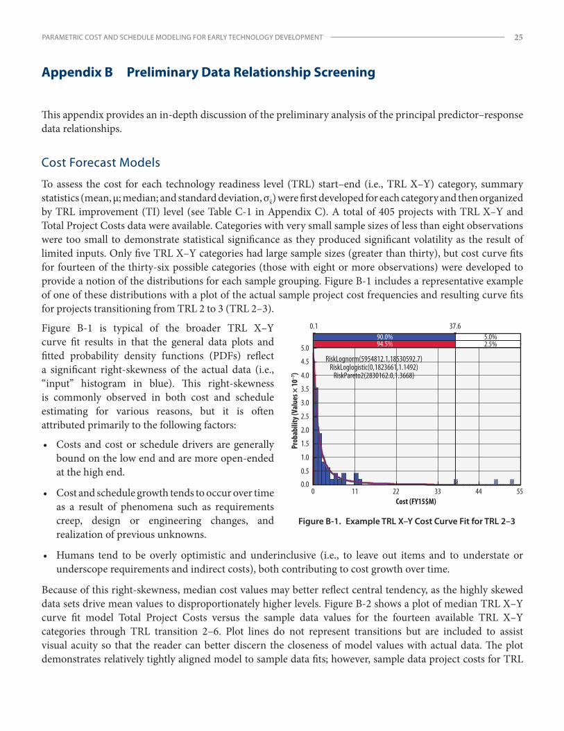
PARAMETRIC COST AND SCHEDULE MODELING FOR EARLY TECHNOLOGY DEVELOPMENT 25
Appendix B Preliminary Data Relationship Screening
This appendix provides an in-depth discussion of the preliminary analysis of the principal predictor–response data relationships.
Cost Forecast Models
To assess the cost for each technology readiness level (TRL) start–end (i.e., TRL X–Y) category, summary statistics (mean, μ; median; and standard deviation, σxr) were first developed for each category and then organized by TRL improvement (TI) level (see Table C-1 in Appendix C). A total of 405 projects with TRL X–Y and Total Project Costs data were available. Categories with very small sample sizes of less than eight observations were too small to demonstrate statistical significance as they produced significant volatility as the result of limited inputs. Only five TRL X–Y categories had large sample sizes (greater than thirty), but cost curve fits for fourteen of the thirty-six possible categories (those with eight or more observations) were developed to provide a notion of the distributions for each sample grouping. Figure B-1 includes a representative example of one of these distributions with a plot of the actual sample project cost frequencies and resulting curve fits for projects transitioning from TRL 2 to 3 (TRL 2–3).
Figure B-1 is typical of the broader TRL X–Y curve fit results in that the general data plots and fitted probability density functions (PDFs) reflect a significant right-skewness of the actual data (i.e., “input” histogram in blue). This right-skewness is commonly observed in both cost and schedule estimating for various reasons, but it is often attributed primarily to the following factors:
• Costs and cost or schedule drivers are generally bound on the low end and are more open-ended at the high end.
• Cost and schedule growth tends to occur over time as a result of phenomena such as requirements creep, design or engineering changes, and realization of previous unknowns.
• Humans tend to be overly optimistic and underinclusive (i.e., to leave out items and to understate or underscope requirements and indirect costs), both contributing to cost growth over time.
Because of this right-skewness, median cost values may better reflect central tendency, as the highly skewed data sets drive mean values to disproportionately higher levels. Figure B-2 shows a plot of median TRL X–Y curve fit model Total Project Costs versus the sample data values for the fourteen available TRL X–Y categories through TRL transition 2–6. Plot lines do not represent transitions but are included to assist visual acuity so that the reader can better discern the closeness of model values with actual data. The plot demonstrates relatively tightly aligned model to sample data fits; however, sample data project costs for TRL
5.0%94.5% 2.5%
0.1 37.6
0 11 22 33 44 550.0
0.5
1.0
1.5
2.0
2.5
3.0
3.5
4.0
4.5
5.0
Prob
abili
ty (V
alue
s × 10
–7)
Cost (FY15$M)
RiskLognorm(5954812.1,18530592.7)RiskLoglogistic(0,1823661,1.1492)
RiskPareto2(2830162.0,1.3668)
90.0%
Figure B-1. Example TRL X–Y Cost Curve Fit for TRL 2–3
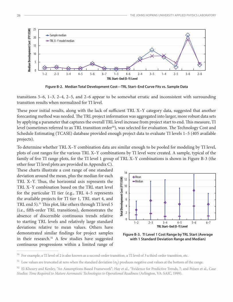
THE JOHNS HOPKINS UNIVERSITY APPLIED PHYSICS LABORATORY26
transitions 5–6, 1–3, 2–4, 2–5, and 2–6 appear to be somewhat erratic and inconsistent with surrounding transition results when normalized for TI level.
These poor initial results, along with the lack of sufficient TRL X–Y category data, suggested that another forecasting method was needed. The TRL project information was aggregated into larger, more robust data sets by applying a parameter that captures the overall TRL level increase from project start to end. This measure, TI level (sometimes referred to as TRL transition order30), was selected for evaluation. The Technology Cost and Schedule Estimating (TCASE) database provided enough project data to evaluate TI levels 1–5 (405 available projects).
To determine whether TRL X–Y combination data are similar enough to be pooled for modeling by TI level, plots of cost ranges for the various TRL X–Y combinations by TI level were created. A sample, typical of the family of five TI range plots, for the TI level 1 group of TRL X–Y combinations is shown in Figure B-3 (the other four TI level plots are provided in Appendix C). These charts illustrate a cost range of one standard deviation around the mean, plus the median for each TRL X–Y. Thus, the horizontal axis represents the TRL X–Y combination based on the TRL start level for the particular TI tier (e.g., TRL 4–5 represents the available projects for TI tier 1, TRL start 4, and TRL end 5).31 This plot, like others through TI level 5 (i.e., fifth-order TRL transitions), demonstrates the absence of discernible continuous trends relative to starting TRL levels and relatively large standard deviations relative to mean values. Others have demonstrated similar findings for project samples in their research.32 A few studies have suggested continuous progressions within a limited range of
30 For example, a TI level of 2 is also known as a second-order transition, a TI level of 3 a third-order transition, etc.31 Low values are truncated at zero when the standard deviation (σxr) produces negative cost values at the bottom of the range.32 El-Khoury and Kenley, “An Assumptions-Based Framework”; Hay et al., “Evidence for Predictive Trends, 7; and Peisen et al., Case Studies: Time Required to Mature Aeronautic Technologies to Operational Readiness (Arlington, VA: SAIC, 1999).
0
5
10
15
20
25
1–2 2–3 3–4 4–5 5–6 6–7 1–3 2–4 3–54–6 1–4 2–5 3–6 2–6
Med
ian
Deve
lopm
ent C
ost
(FY1
5$M
)
TRL Start–End (X–Y) Level
Sample median
TRL X–Y model median
Figure B-2. Median Total Development Cost—TRL Start–End Curve Fits vs. Sample Data
0
2
4
6
8
10
12
14
2–3 3–4 4–5 5–6 6–7
Tota
l Dev
elop
men
t Cos
t (FY
15$M
)
TRL Start–End (X–Y) Level
MeanMedian
1–2
Figure B-3. TI Level 1 Cost Range by TRL Start (Average with 1 Standard Deviation Range and Median)
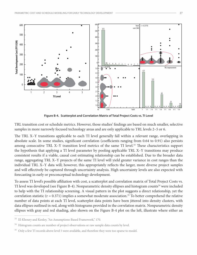
PARAMETRIC COST AND SCHEDULE MODELING FOR EARLY TECHNOLOGY DEVELOPMENT 27
TRL transition cost or schedule metrics. However, those studies’ findings are based on much smaller, selective samples in more narrowly focused technology areas and are only applicable to TRL levels 2–5 or 6.
The TRL X–Y transitions applicable to each TI level generally fall within a relevant range, overlapping in absolute scale. In some studies, significant correlation (coefficients ranging from 0.64 to 0.91) also persists among consecutive TRL X–Y transition level metrics of the same TI level.33 These characteristics support the hypothesis that applying a TI level parameter by pooling applicable TRL X–Y transitions may produce consistent results if a viable, causal cost estimating relationship can be established. Due to the broader data range, aggregating TRL X–Y projects of the same TI level will yield greater variance in cost ranges than the individual TRL X–Y data will; however, this appropriately reflects the larger, more diverse project samples and will effectively be captured through uncertainty analysis. High uncertainty levels are also expected with forecasting in early or preconceptual technology development.
To assess TI level’s possible affiliation with cost, a scatterplot and correlation matrix of Total Project Costs vs. TI level was developed (see Figure B-4). Nonparametric density ellipses and histogram counts34 were included to help with the TI relationship screening. A visual pattern in the plot suggests a direct relationship, yet the correlation statistic (r = 0.371) implies a somewhat moderate association.35 To better comprehend the relative number of data points at each TI level, scatterplot data points have been jittered into density clusters, with data ellipses outlined in red, along with histograms provided in the correlation matrix. Nonparametric density ellipses with gray and red shading, also shown on the Figure B-4 plot on the left, illustrate where either an
33 El-Khoury and Kenley, “An Assumptions-Based Framework,” 170.34 Histogram counts are number of project observations or raw sample data counts by level.35 Only a few TI records above level 5 were available, and therefore they were too sparse to model.
51 2 3 4
0
100
200
300
400
500
600
TI Level
Tota
l Dev
elop
men
t Cos
t (FY
15$M
)
500
600
400
300
200
100
0
372
14 5 4 4 2 2 1 0 0 1 1r=0.3710
$0 $600
r = 0.3710
177
0 0 0
133
0 0 0
64
0 0 0
22
0 0 010
1 1.5 2.0 2.5 3.0 3.5 4.0 4.5 5.0
Total cost ($M)
TRL improvement
1.0
1.5
2.0
2.5
3.0
3.5
4.0
4.5
5.0
$200
Figure B-4. Scatterplot and Correlation Matrix of Total Project Costs vs. TI Level
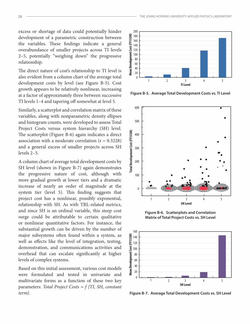
THE JOHNS HOPKINS UNIVERSITY APPLIED PHYSICS LABORATORY28
excess or shortage of data could potentially hinder development of a parametric construction between the variables. These findings indicate a general overabundance of smaller projects across TI levels 2–5, potentially “weighing down” the progressive relationship.
The direct nature of cost’s relationship to TI level is also evident from a column chart of the average total development costs by level (see Figure B-5). Cost growth appears to be relatively nonlinear, increasing at a factor of approximately three between successive TI levels 1–4 and tapering off somewhat at level 5.
Similarly, a scatterplot and correlation matrix of these variables, along with nonparametric density ellipses and histogram counts, were developed to assess Total Project Costs versus system hierarchy (SH) level. The scatterplot (Figure B-6) again indicates a direct association with a moderate correlation (r = 0.3228) and a general excess of smaller projects across SH levels 2–5.
A column chart of average total development costs by SH level (shown in Figure B-7) again demonstrates the progressive nature of cost, although with more gradual growth at lower tiers and a dramatic increase of nearly an order of magnitude at the system tier (level 5). This finding suggests that project cost has a nonlinear, possibly exponential, relationship with SH. As with TRL-related metrics, and since SH is an ordinal variable, this steep cost surge could be attributable to certain qualitative or nonlinear quantitative factors. For instance, the substantial growth can be driven by the number of major subsystems often found within a system, as well as effects like the level of integration, testing, demonstration, and communications activities and overhead that can escalate significantly at higher levels of complex systems.
Based on this initial assessment, various cost models were formulated and tested in univariate and multivariate forms as a function of these two key parameters: Total Project Costs = f {TI, SH, constant term}.
Figure B-5. Average Total Development Costs vs. TI Level
020406080
100120140160180200
1 2 3 4 5
Mea
n Dev
elopm
ent C
ost (
FY15
$M)
TI Level
0
100
200
300
400
500
600
1 2 3 4 5SH Level
Tota
l Dev
elop
men
t Cos
t (FY
15$M
)
Figure B-6. Scatterplots and Correlation Matrix of Total Project Costs vs. SH Level
Figure B-7. Average Total Development Costs vs. SH Level
0
20
40
60
80
100
120
140
160
Mea
n Dev
elopm
ent C
ost (
FY15
$M)
SH Level1 2 3 4 5
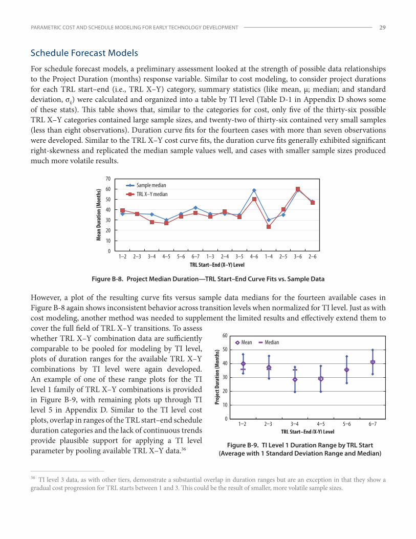
PARAMETRIC COST AND SCHEDULE MODELING FOR EARLY TECHNOLOGY DEVELOPMENT 29
Schedule Forecast Models
For schedule forecast models, a preliminary assessment looked at the strength of possible data relationships to the Project Duration (months) response variable. Similar to cost modeling, to consider project durations for each TRL start–end (i.e., TRL X–Y) category, summary statistics (like mean, μ; median; and standard deviation, σxr
) were calculated and organized into a table by TI level (Table D-1 in Appendix D shows some of these stats). This table shows that, similar to the categories for cost, only five of the thirty-six possible TRL X–Y categories contained large sample sizes, and twenty-two of thirty-six contained very small samples (less than eight observations). Duration curve fits for the fourteen cases with more than seven observations were developed. Similar to the TRL X–Y cost curve fits, the duration curve fits generally exhibited significant right-skewness and replicated the median sample values well, and cases with smaller sample sizes produced much more volatile results.
However, a plot of the resulting curve fits versus sample data medians for the fourteen available cases in Figure B-8 again shows inconsistent behavior across transition levels when normalized for TI level. Just as with cost modeling, another method was needed to supplement the limited results and effectively extend them to cover the full field of TRL X–Y transitions. To assess whether TRL X–Y combination data are sufficiently comparable to be pooled for modeling by TI level, plots of duration ranges for the available TRL X–Y combinations by TI level were again developed. An example of one of these range plots for the TI level 1 family of TRL X–Y combinations is provided in Figure B-9, with remaining plots up through TI level 5 in Appendix D. Similar to the TI level cost plots, overlap in ranges of the TRL start–end schedule duration categories and the lack of continuous trends provide plausible support for applying a TI level parameter by pooling available TRL X–Y data.36
36 TI level 3 data, as with other tiers, demonstrate a substantial overlap in duration ranges but are an exception in that they show a gradual cost progression for TRL starts between 1 and 3. This could be the result of smaller, more volatile sample sizes.
0
10
20
30
40
50
60
1–2 2–3 3–4 4–5 5–6 6–7
Proj
ect D
urat
ion
(Mon
ths)
TRL Start–End (X-Y) Level
Mean Median
Figure B-9. TI Level 1 Duration Range by TRL Start (Average with 1 Standard Deviation Range and Median)
0
10
20
30
40
50
60
70
1–2 2–3 3–4 4–5 5–6 6–7 1–3 2–4 3–5 4–6 1–4 2–5 3–6 2–6
Mea
n Du
ratio
n (M
onth
s)
TRL Start–End (X–Y) Level
Sample medianTRL X–Y median
Figure B-8. Project Median Duration—TRL Start–End Curve Fits vs. Sample Data
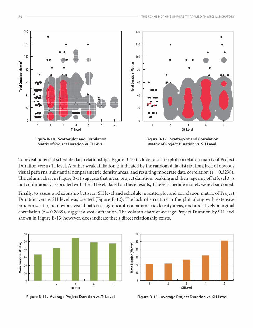
THE JOHNS HOPKINS UNIVERSITY APPLIED PHYSICS LABORATORY30
To reveal potential schedule data relationships, Figure B-10 includes a scatterplot correlation matrix of Project Duration versus TI level. A rather weak affiliation is indicated by the random data distribution, lack of obvious visual patterns, substantial nonparametric density areas, and resulting moderate data correlation (r = 0.3238). The column chart in Figure B-11 suggests that mean project duration, peaking and then tapering off at level 3, is not continuously associated with the TI level. Based on these results, TI level schedule models were abandoned.
Finally, to assess a relationship between SH level and schedule, a scatterplot and correlation matrix of Project Duration versus SH level was created (Figure B-12). The lack of structure in the plot, along with extensive random scatter, no obvious visual patterns, significant nonparametric density areas, and a relatively marginal correlation (r = 0.2869), suggest a weak affiliation. The column chart of average Project Duration by SH level shown in Figure B-13, however, does indicate that a direct relationship exists.
Tota
l Dur
atio
n (M
onth
s)
120
140
100
80
60
40
20
01 2 3 4 5 6 9
TI Level
Figure B-10. Scatterplot and Correlation Matrix of Project Duration vs. TI Level
Figure B-11. Average Project Duration vs. TI Level
0
10
20
30
1 2 3 4 5
Mea
n Du
ratio
n (M
onth
s)
TI Level
50
40
60
Figure B-13. Average Project Duration vs. SH Level
0
10
20
30
40
50
60
1 2 3 4 5
Mea
n Du
ratio
n (M
onth
s)
SH Level
20
0
40
60
80
100
120
140
1 2 3 4 5
Tota
l Dur
atio
n (M
onth
s)SH Level
Figure B-12. Scatterplot and Correlation Matrix of Project Duration vs. SH Level
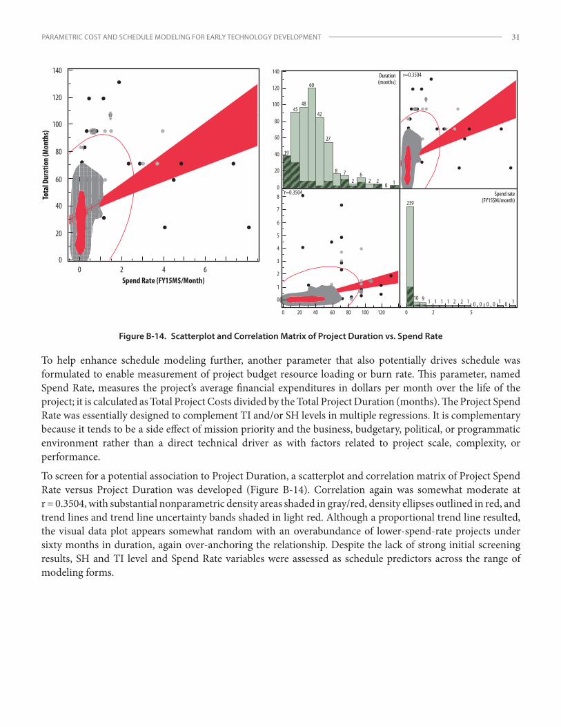
PARAMETRIC COST AND SCHEDULE MODELING FOR EARLY TECHNOLOGY DEVELOPMENT 31
To help enhance schedule modeling further, another parameter that also potentially drives schedule was formulated to enable measurement of project budget resource loading or burn rate. This parameter, named Spend Rate, measures the project’s average financial expenditures in dollars per month over the life of the project; it is calculated as Total Project Costs divided by the Total Project Duration (months). The Project Spend Rate was essentially designed to complement TI and/or SH levels in multiple regressions. It is complementary because it tends to be a side effect of mission priority and the business, budgetary, political, or programmatic environment rather than a direct technical driver as with factors related to project scale, complexity, or performance.
To screen for a potential association to Project Duration, a scatterplot and correlation matrix of Project Spend Rate versus Project Duration was developed (Figure B-14). Correlation again was somewhat moderate at r = 0.3504, with substantial nonparametric density areas shaded in gray/red, density ellipses outlined in red, and trend lines and trend line uncertainty bands shaded in light red. Although a proportional trend line resulted, the visual data plot appears somewhat random with an overabundance of lower-spend-rate projects under sixty months in duration, again over-anchoring the relationship. Despite the lack of strong initial screening results, SH and TI level and Spend Rate variables were assessed as schedule predictors across the range of modeling forms.
0
20
40
60
80
100
120
140
0
1
2
3
4
5
6
7
8
19
4548
60
42
27
8 72
62 2
0 1
r=0.3504
0 20 40 60 80 100 120
r=0.3504
239
10 9 1 1 1 1 2 2 1 0 0 0 0 1 0 1
0 2 5
Duration(months)
Spend rate(FY15$M/month)
20
0
40
60
80
100
120
140
0 642Spend Rate (FY15M$/Month)
Tota
l Dur
atio
n (M
onth
s)
Figure B-14. Scatterplot and Correlation Matrix of Project Duration vs. Spend Rate

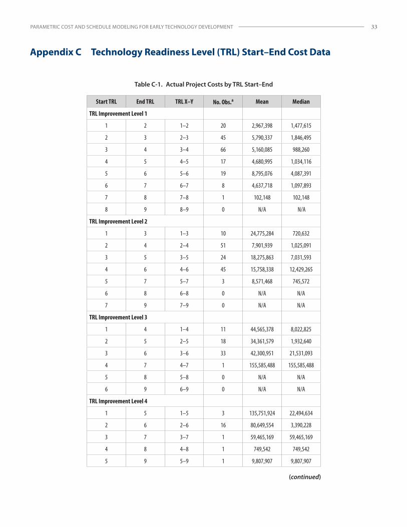
PARAMETRIC COST AND SCHEDULE MODELING FOR EARLY TECHNOLOGY DEVELOPMENT 33
Appendix C Technology Readiness Level (TRL) Start–End Cost Data
Table C-1. Actual Project Costs by TRL Start–End
Start TRL End TRL TRL X–Y No. Obs.a Mean Median
TRL Improvement Level 1
1 2 1–2 20 2,967,398 1,477,615
2 3 2–3 45 5,790,337 1,846,495
3 4 3–4 66 5,160,085 988,260
4 5 4–5 17 4,680,995 1,034,116
5 6 5–6 19 8,795,076 4,087,391
6 7 6–7 8 4,637,718 1,097,893
7 8 7–8 1 102,148 102,148
8 9 8–9 0 N/A N/A
TRL Improvement Level 2
1 3 1–3 10 24,775,284 720,632
2 4 2–4 51 7,901,939 1,025,091
3 5 3–5 24 18,275,863 7,031,593
4 6 4–6 45 15,758,338 12,429,265
5 7 5–7 3 8,571,468 745,572
6 8 6–8 0 N/A N/A
7 9 7–9 0 N/A N/A
TRL Improvement Level 3
1 4 1–4 11 44,565,378 8,022,825
2 5 2–5 18 34,361,579 1,932,640
3 6 3–6 33 42,300,951 21,531,093
4 7 4–7 1 155,585,488 155,585,488
5 8 5–8 0 N/A N/A
6 9 6–9 0 N/A N/A
TRL Improvement Level 4
1 5 1–5 3 135,751,924 22,494,634
2 6 2–6 16 80,649,554 3,390,228
3 7 3–7 1 59,465,169 59,465,169
4 8 4–8 1 749,542 749,542
5 9 5–9 1 9,807,907 9,807,907
(continued)
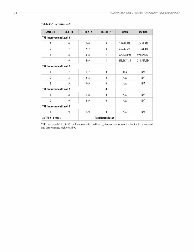
THE JOHNS HOPKINS UNIVERSITY APPLIED PHYSICS LABORATORY34
Start TRL End TRL TRL X–Y No. Obs.a Mean Median
TRL Improvement Level 5
1 6 1–6 5 18,095,038 2,451,542
2 7 2–7 3 45,435,638 1,244,334
3 8 3–8 1 594,678,801 594,678,801
4 9 4–9 1 213,567,134 213,567,134
TRL Improvement Level 6
1 7 1–7 0 N/A N/A
2 8 2–8 0 N/A N/A
3 9 3–9 0 N/A N/A
TRL Improvement Level 7 0
1 8 1–8 0 N/A N/A
2 9 2–9 0 N/A N/A
TRL Improvement Level 8
1 9 1–9 0 N/A N/A
36 TRL X–Y types Total Records 405
a TRL start–end (TRL X–Y) combinations with less than eight observations were too limited to be assessed and demonstrated high volatility.
Table C-1 (continued)
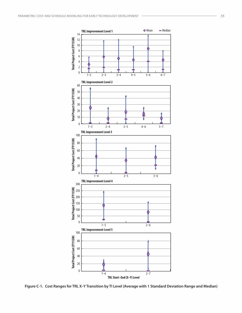
PARAMETRIC COST AND SCHEDULE MODELING FOR EARLY TECHNOLOGY DEVELOPMENT 35
Tota
l Pro
ject
Cost
(FY1
5$M
)To
tal P
roje
ct Co
st (F
Y15$
M)
Tota
l Pro
ject
Cost
(FY1
5$M
)To
tal P
roje
ct Co
st (F
Y15$
M)
Tota
l Pro
ject
Cost
(FY1
5$M
)
TRL Start–End (X–Y) Level
1–2 2–3 4–5 5–6 6–70
2
4
6
8
10
12
14Mean MedianTRL Improvement Level 1
3–4
1–3 2–4 3–5 4–6 5–70
10
20
30
40
50
60TRL Improvement Level 2
0
20
40
60
80
100
1–4 2–5 3–6
TRL Improvement Level 3
TRL Improvement Level 5
0
20
40
60
80
100
1–6 2–7
0
50
100
150
200
250
300
1–5 2–6
TRL Improvement Level 4
Figure C-1. Cost Ranges for TRL X–Y Transition by TI Level (Average with 1 Standard Deviation Range and Median)

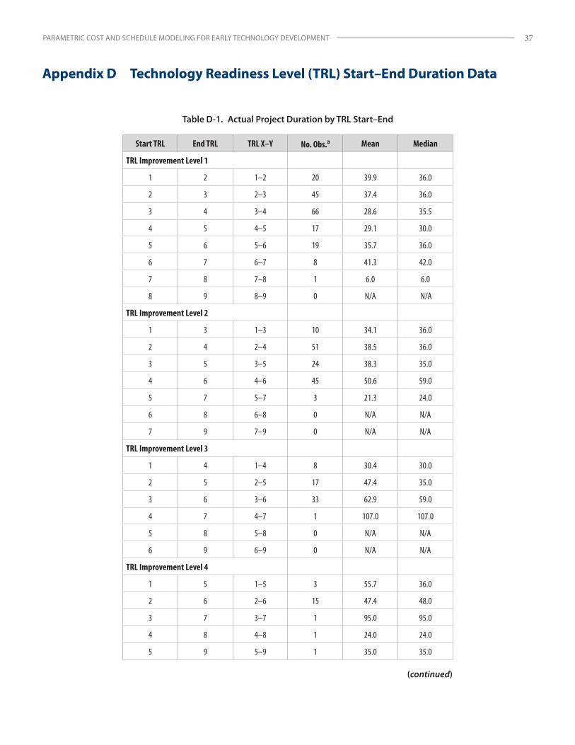
PARAMETRIC COST AND SCHEDULE MODELING FOR EARLY TECHNOLOGY DEVELOPMENT 37
Appendix D Technology Readiness Level (TRL) Start–End Duration Data
Table D-1. Actual Project Duration by TRL Start–End
Start TRL End TRL TRL X–Y No. Obs.a Mean Median
TRL Improvement Level 1
1 2 1–2 20 39.9 36.0
2 3 2–3 45 37.4 36.0
3 4 3–4 66 28.6 35.5
4 5 4–5 17 29.1 30.0
5 6 5–6 19 35.7 36.0
6 7 6–7 8 41.3 42.0
7 8 7–8 1 6.0 6.0
8 9 8–9 0 N/A N/A
TRL Improvement Level 2
1 3 1–3 10 34.1 36.0
2 4 2–4 51 38.5 36.0
3 5 3–5 24 38.3 35.0
4 6 4–6 45 50.6 59.0
5 7 5–7 3 21.3 24.0
6 8 6–8 0 N/A N/A
7 9 7–9 0 N/A N/A
TRL Improvement Level 3
1 4 1–4 8 30.4 30.0
2 5 2–5 17 47.4 35.0
3 6 3–6 33 62.9 59.0
4 7 4–7 1 107.0 107.0
5 8 5–8 0 N/A N/A
6 9 6–9 0 N/A N/A
TRL Improvement Level 4
1 5 1–5 3 55.7 36.0
2 6 2–6 15 47.4 48.0
3 7 3–7 1 95.0 95.0
4 8 4–8 1 24.0 24.0
5 9 5–9 1 35.0 35.0
(continued)
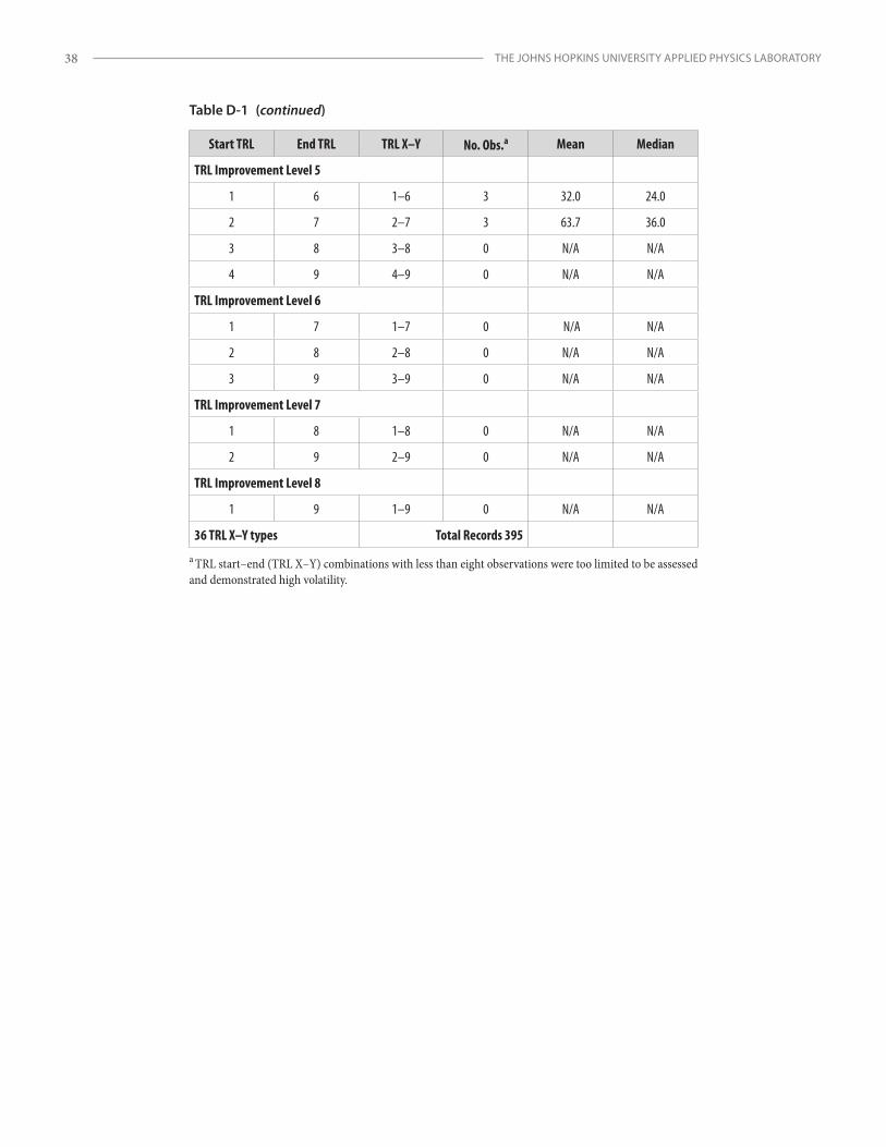
THE JOHNS HOPKINS UNIVERSITY APPLIED PHYSICS LABORATORY38
Start TRL End TRL TRL X–Y No. Obs.a Mean Median
TRL Improvement Level 5
1 6 1–6 3 32.0 24.0
2 7 2–7 3 63.7 36.0
3 8 3–8 0 N/A N/A
4 9 4–9 0 N/A N/A
TRL Improvement Level 6
1 7 1–7 0 N/A N/A
2 8 2–8 0 N/A N/A
3 9 3–9 0 N/A N/A
TRL Improvement Level 7
1 8 1–8 0 N/A N/A
2 9 2–9 0 N/A N/A
TRL Improvement Level 8
1 9 1–9 0 N/A N/A
36 TRL X–Y types Total Records 395
a TRL start–end (TRL X–Y) combinations with less than eight observations were too limited to be assessed and demonstrated high volatility.
Table D-1 (continued)
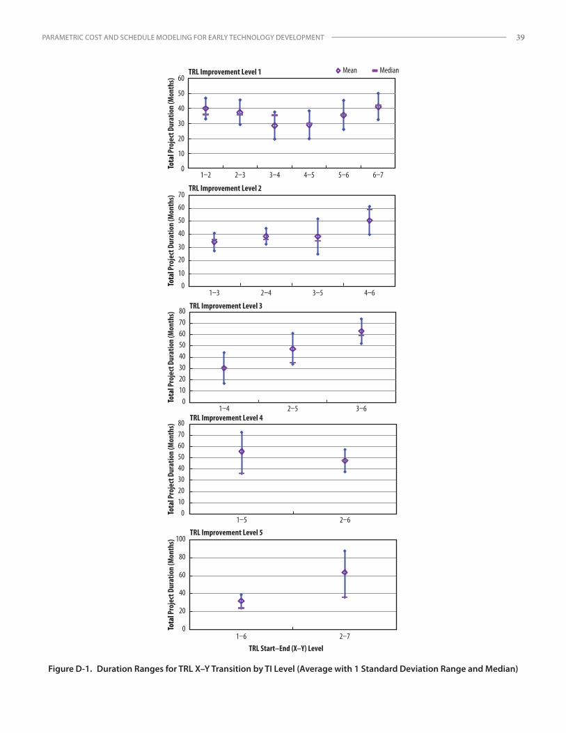
PARAMETRIC COST AND SCHEDULE MODELING FOR EARLY TECHNOLOGY DEVELOPMENT 39
Tota
l Pro
ject
Dur
atio
n (M
onth
s)To
tal P
roje
ct D
urat
ion
(Mon
ths)
Tota
l Pro
ject
Dur
atio
n (M
onth
s)To
tal P
roje
ct D
urat
ion
(Mon
ths)
Tota
l Pro
ject
Dur
atio
n (M
onth
s)1–2 2–3 3–4 4–5 5–6 6–7
0
10
20
30
40
50
60TRL Improvement Level 1
0
10
20
30
40
50
60
70
1–3 2–4 3–5 4–6
TRL Improvement Level 2
01020304050607080
1–4 2–5 3–6
TRL Improvement Level 3
01020304050607080
TRL Improvement Level 4
1–5 2–6
0
20
40
60
80
100
1–6 2–7
TRL Improvement Level 5
TRL Start–End (X–Y) Level
Mean Median
Figure D-1. Duration Ranges for TRL X–Y Transition by TI Level (Average with 1 Standard Deviation Range and Median)

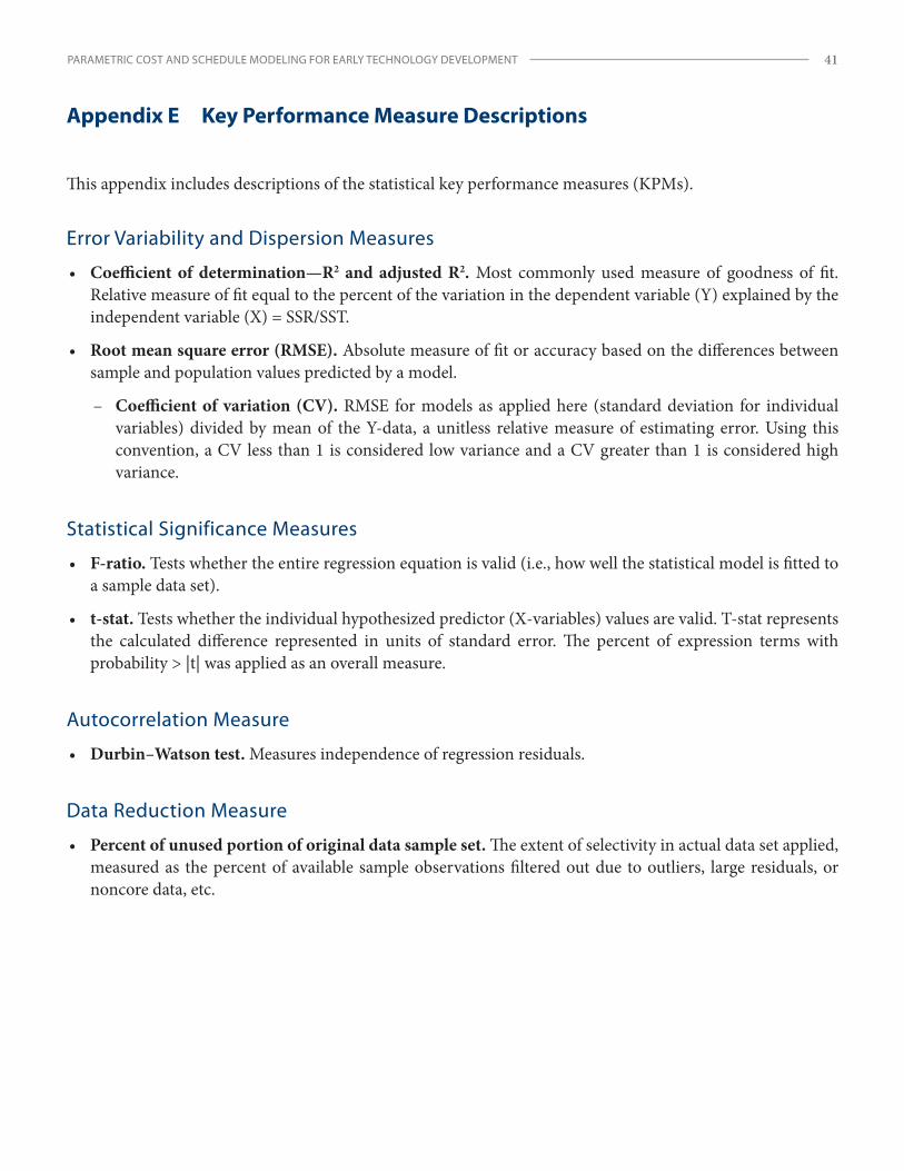
PARAMETRIC COST AND SCHEDULE MODELING FOR EARLY TECHNOLOGY DEVELOPMENT 41
Appendix E Key Performance Measure Descriptions
This appendix includes descriptions of the statistical key performance measures (KPMs).
Error Variability and Dispersion Measures
• Coefficient of determination—R2 and adjusted R2. Most commonly used measure of goodness of fit. Relative measure of fit equal to the percent of the variation in the dependent variable (Y) explained by the independent variable (X) = SSR/SST.
• Root mean square error (RMSE). Absolute measure of fit or accuracy based on the differences between sample and population values predicted by a model.
– Coefficient of variation (CV). RMSE for models as applied here (standard deviation for individual variables) divided by mean of the Y-data, a unitless relative measure of estimating error. Using this convention, a CV less than 1 is considered low variance and a CV greater than 1 is considered high variance.
Statistical Significance Measures
• F-ratio. Tests whether the entire regression equation is valid (i.e., how well the statistical model is fitted to a sample data set).
• t-stat. Tests whether the individual hypothesized predictor (X-variables) values are valid. T-stat represents the calculated difference represented in units of standard error. The percent of expression terms with probability > |t| was applied as an overall measure.
Autocorrelation Measure
• Durbin–Watson test. Measures independence of regression residuals.
Data Reduction Measure
• Percent of unused portion of original data sample set. The extent of selectivity in actual data set applied, measured as the percent of available sample observations filtered out due to outliers, large residuals, or noncore data, etc.


PARAMETRIC COST AND SCHEDULE MODELING FOR EARLY TECHNOLOGY DEVELOPMENT 43
Acknowledgments
Thanks to Matt Schaffer and Rodney Yerger for their constructive reviews of drafts and suggestions that helped focus key aspects of the report. Thanks also to Marc Greenberg, Eric Plumer, and Doug Comstock of NASA Headquarters and Kirk Cole of the NASA Langley Research Center Research Directorate for providing access to and background for the TCASE database, which was pivotal to this effort.
About the Author
Chuck Alexander is a Senior Professional Staff member in the Cost Analysis Section of JHU/APL’s National Security Analysis Department. He performs economic and cost analysis for a variety of sponsors across a range of applications, technologies, and system environments. He has over 30 years of professional experience in cost engineering, investment decision analysis, business operations, technology management, and management consulting. Mr. Alexander is a licensed professional engineer (PE), a certified public accountant (CPA), and a former certified cost estimator/analyst (CCE/A). He holds a BS in mechanical engineering from Clarkson University and an MBA in finance from the William & Mary Mason School of Business.

PARAMETRIC COST AND SCHEDULE MODELING FOR EARLY TECHNOLOGY DEVELOPMENT 45
Bibliography
Anderson, J. A. “Regression and Ordered Categorical Variables.” Journal of the Royal Statistical Society Series B 46, no. 1 (1984): 1–30.
Berry, William D. Understanding Regression Assumptions. Quantitative Applications in the Social Sciences Series. Newbury Park, CA: Sage, 1993.
Cole, Stuart K., John D. Reeves, Julie A. Williams-Byrd, Marc Greenberg, Doug Comstock, John R. Olds, Jon Wallace, Dominic DePasquale, and Mark Schaffer. Technology Estimating: A Process to Determine Cost and Schedule of Space Technology R&D. NASA/TP–2013-218145. Washington, DC: NASA, 2013.
Conrow, Edmund H. “Estimating Technology Readiness Level Coefficients.” In Proceedings of the AIAA SPACE 2009 Conference & Exposition, 1–9. Reston, VA: AIAA, 2009.
Curran, Richard, Srinivasan Raghunathan, and Mark Price. “Review of Aerospace Engineering Cost Modeling: The Genetic Causal Approach.” Process in Aerospace Sciences 40, no. 8 (2004): 487–534.
Director, Research Directorate, Office of the Director, Defense Research and Engineering. DoD Technology Readiness Assessment (TRA) Deskbook. Washington, DC: Department of Defense, July 2009.
El-Khoury, Bernard, and C. Robert Kenley. “An Assumptions-Based Framework for TRL-Based Cost and Schedule Models.” Journal of Cost Analysis and Parametrics 7, no. 3 (2014): 160–179.
Gertheiss, Jan, and Gerhard Tutz. “Penalized Regression with Ordinal Predictors.” International Statistical Review 77, no. 3 (2009): 345–365.
Hay, Jason, J. D. Reeves, Elaine Gresham, Julie Williams-Byrd, Emma Hinds, and Jillian Taylor. “Evidence for Predictive Trends in Technology Readiness Level Transition Metrics.” In Proceedings of the AIAA SPACE Conference and Exposition, AIAA 2013-5369. Reston, VA: AIAA, 2013.
Homeland Security Institute. Department of Homeland Security Science and Technology Readiness Level Calculator (ver. 1.1): Final Report and User’s Manual. Washington, DC: Department of Homeland Security, September 30, 2009.
Jones, Mark B., Phil F. Webb, Mark D. Summers, and Paul Baguley. “COTECHMO: The Constructive Technology Development Cost Model.” Journal of Cost Analysis and Parametrics 7, no. 1 (2014): 48–61.
Malone, Patrick, Roy Smoker, Henry Apgar, and Lawrence Wolfarth. “The Application of TRL Metrics to Existing Cost Prediction Models: A Practitioners Guide to Applying Cost Correction Factors to Technology.” In Proceedings of the 2011 Aerospace Conference, 1–12. Piscataway, NJ: IEEE, 2011.
Mankins, John C. Technology Readiness Levels. Washington, DC: NASA, 1995.
Peisen, Deborah J., Catherine L. Schultz, Richard S. Golaszewski, David B. Ballard, and John J. Smith. Case Studies: Time Required to Mature Aeronautic Technologies to Operational Readiness. Arlington, VA: SAIC, 1999.

THE JOHNS HOPKINS UNIVERSITY APPLIED PHYSICS LABORATORY46
Sanchez, Ruben. Technology Readiness Assessment Guide. DOE G 413.3-4A. Washington, DC: Department of Energy, September 2011.
Sauser, Brian, Jose Ramirez-Marquez, Dinesh Verma, and Ryan Gove. “From TRL to SRL: The Concept of Systems Readiness Levels.” In Proceedings of the Conference on Systems Engineering Research, paper 126. Los Angeles: Conference on Systems Engineering Research, 2006.
Sauser, Brian, Jose E. Ramirez-Marquez, Romulo Magnaye, and Weiping Tan. “A Systems Approach to Expanding the TRL Level within Defense Acquisition.” International Journal of Defense Acquisition Management 1 (2008): 39–58.
Shermon, Dale, and Catherine Barnaby. “Macro-Parametrics and the Applications of Multi-Colinearity and Bayesian to Enhance Early Cost Modeling.” In Proceedings of the International Cost Estimating and Analysis Association 2015 Professional Development & Training Workshop. Annandale, VA: ICEAA, 2015.
Smoker, Roy E., and Sean Smith. “System Cost Growth Associated with TRL.” Journal of Parametrics 26, no. 1 (2007): 8–38.
SpaceWorks Enterprises, Inc.. TCASE Technology Cost and Schedule Estimation Tool User Training Presentation, Rev5 (2015-03-19). Atlanta: SpaceWorks, 2015.
Stahl, H. Philip, Kyle Stephens, Todd Henrichs, Christian Smart, and Frank A. Prince. “Single-Variable Parametric Cost Models for Space Telescopes.” Optical Engineering 49, no. 7 (2010): 073006.
Stauner, Nick. February 21, 2014. Response to “Effect of Two Demographic IVs on Survey Answers (Likert Scale).” CrossValidated, http://stats.stackexchange.com/questions/86923/effect-of-two-demographic-ivs-on-survey-answers-likert-scale.
US General Accounting Office. Best Practices: Better Management of Technology Development Can Improve Weapon System. Report to the Chairman and Ranking Minority Member, Subcommittee on Readiness and Management Support, Committee on Armed Services, U.S. Senate. GAO/NSIAD-99-162. Washington, DC: GAO, July 1999.
US Government Accountability Office. Technology Readiness Assessment Guide: Best Practices for Evaluating the Readiness of Technology for Use in Acquisition Programs and Projects. GAO-16-410G. Washington, DC: GAO, August 2016.


Research NoteNational Security Report
PARAMETRIC
MODELING FOR EARLY TECHNOLOGY DEVELOPMENT
COST AND SCHEDULE
Chuck Alexander
NSR_11x17_Cover_CostModeling_v8.indd 1 11/20/17 3:15 PM