Journal of Mathematical Finance, 2017, 7, 121-143 http://www.scirp.org/journal/jmf

ISSN Online: 2162-2442 ISSN Print: 2162-2434

DOI: 10.4236/jmf.2017.71007 February 6, 2017

Modeling Exchange Rate Volatility: Application of the GARCH and EGARCH Models

Manamba Epaphra

Department of Accounting and Finance, Institute of Accountancy Arusha, Arusha, Tanzania

Abstract Policy makers need accurate forecasts about future values of exchange rates. This is due to the fact that exchange rate volatility is a useful measure of un-certainty about the economic environment of a country. This paper applies univariate nonlinear time series analysis to the daily (TZS/USD) exchange rate data spanning from January 4, 2009 to July 27, 2015 to examine the behavior of exchange rate in Tanzania. To capture the symmetry effect in exchange rate data, the paper applies both ARCH and GARCH models. Also, the paper em-ploys exponential GARCH (EGARCH) model to capture the asymmetry in volatility clustering and the leverage effect in exchange rate. The paper reveals that exchange rate series exhibits the empirical regularities such as clustering volatility, nonstationarity, non-normality and serial correlation that justify the application of the ARCH methodology. The results also suggest that exchange rate behavior is generally influenced by previous information about exchange rate. This also implies that previous day’s volatility in exchange rate can affect current volatility of exchange rate. In addition, the estimate for asymmetric volatility suggests that positive shocks imply a higher next period conditional variance than negative shocks of the same sign. The main policy implication of these results is that since exchange rate volatility (exchange-rate risk) may increase transaction costs and reduce the gains to international trade, know-ledge of exchange rate volatility estimation and forecasting is important for asset pricing and risk management.

Keywords Exchange Rate Volatility, Heteroscedasticity, Leverage Effect, GARCH Models

1. Introduction

Financial time series such as exchange rate often exhibits the phenomenon of volatility clustering, that is, periods in which its prices show wide swings for an

How to cite this paper: Epaphra, M. (2017) Modeling Exchange Rate Volatility: Application of the GARCH and EGARCH Models. Journal of Mathematical Finance, 7, 121-143. https://doi.org/10.4236/jmf.2017.71007 Received: December 14, 2016 Accepted: February 3, 2017 Published: February 6, 2017 Copyright © 2017 by author and Scientific Research Publishing Inc. This work is licensed under the Creative Commons Attribution International License (CC BY 4.0). http://creativecommons.org/licenses/by/4.0/

Open Access

M. Epaphra

122

extended time period followed by periods in which there is calm (Gujarati & Porter [1]). This volatility of exchange rates, particularly after the fall of the Bretton Woods agreements has been a constant source of concern for both poli-cymakers and academics (Héricourt & Poncet, [2]). Indeed, knowledge of vola-tility is of crucial importance because exchange-rate risk may increase transac-tion costs and reduce the gains to international trade.

The fact that Tanzania has gone through the floating exchange rate regime since early 1990s and that currently, the country adheres to the IMF convention of free current account convertibility and transfer; variations in an exchange rate has the potential to affect country’s monetary policies and economic perfor-mance. In addition, there are greater potential vulnerabilities and risks to the stability of financial system in the country following a rapid growth in the vo-lume of financial transactions, increased complexity of financial markets and a more interconnected global economy. Thus, policymakers are interested in measuring exchange volatility to learn about market expectations and uncer-tainty about policy. For example, understanding and estimating exchange vola-tility is important for asset pricing, portfolio allocation, and risk management (Erdemlioglu et al. [3]).

The analysis of financial data has received considerable attention in the litera-ture over the last two decades. Several models have been suggested for capturing special features of financial data, and most of these models have the property that the conditional variance depends on the past. Well known and frequently applied models to estimate exchange rate volatility are the autoregressive condi-tional heteroscedastic (ARCH) model, advanced by Engle [4] and generalized autoregressive conditional heteroskedastic (GARCH) model, developed inde-pendently by Bollerslev [5] and Taylor [6]. These models are applied to account for characteristics of exchange rate volatility such as dynamics of conditional heteroscedasticity. In particular, this class of models has been used to forecast fluctuations in commodities, securities and exchange rates.

The main objective of this paper is to measure the characteristics of exchange volatility including volatility clustering and leverage effect using the ARCH- GARCH and EGARCH time series models. The paper also determines the accu-racy and forecasting future of the models. To accomplish this, the paper consid-ers TZS/USD exchange rate for the 1593 daily observations. For this sequence, the paper considers changes in the daily logarithmic exchange rates. That is, if

tx is the exchange rate at time t , the sequence of exchange rates is trans-formed as follows:

( ) ( )11

log log logtt t t

t

xr x x

x −−

= = −

(1)

where tr is known as the log price relative at time t . Volatility, as measured by the standard deviation or variance of returns, is of-

ten used as a crude measure of the total risk of financial assets. Many val-ue-at-risk models for measuring market risk require the estimation or forecast of a volatility parameter. This paper is expected to provide knowledge on modeling

M. Epaphra

123

exchange rate volatility in developing countries such as Tanzania and it is also expected to contribute to policy making through developing a model which can be used to forecast exchange rate and thus, guides policy makers in formulating macroeconomic policies.

The paper contributes to the existing literature in two ways. First, the current paper explains volatility modeling using recent daily returns. The paper applies both GARCH and the EGARCH models to capture both symmetry and asym-metry in volatility clustering. To the best of my knowledge, while there are stu-dies on the volatility of exchange rate indices in the literature, scholars have not yet modeled exchange rate volatility clustering in Tanzania using recent daily data.

2. Stylized Facts 2.1. Clustering Volatility and Leverage Effects

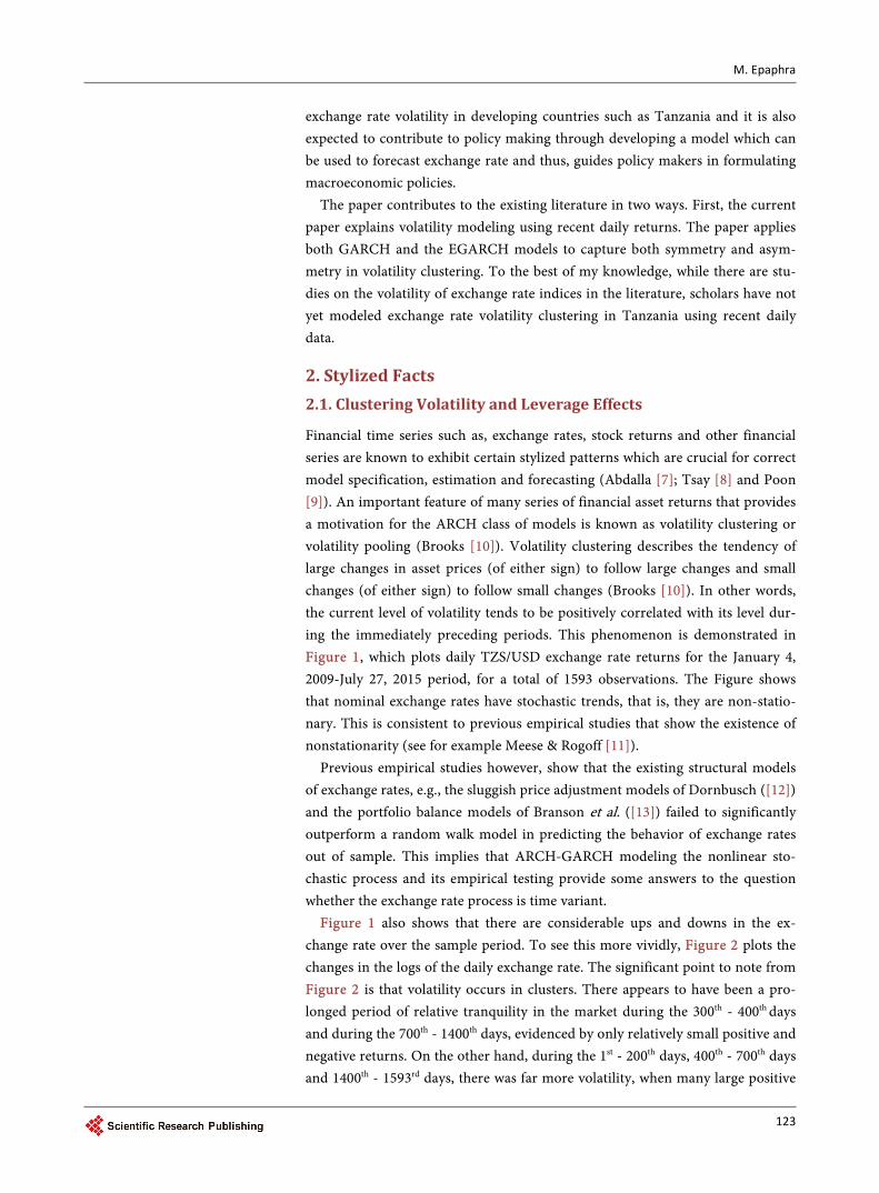
Financial time series such as, exchange rates, stock returns and other financial series are known to exhibit certain stylized patterns which are crucial for correct model specification, estimation and forecasting (Abdalla [7]; Tsay [8] and Poon [9]). An important feature of many series of financial asset returns that provides a motivation for the ARCH class of models is known as volatility clustering or volatility pooling (Brooks [10]). Volatility clustering describes the tendency of large changes in asset prices (of either sign) to follow large changes and small changes (of either sign) to follow small changes (Brooks [10]). In other words, the current level of volatility tends to be positively correlated with its level dur-ing the immediately preceding periods. This phenomenon is demonstrated in Figure 1, which plots daily TZS/USD exchange rate returns for the January 4, 2009-July 27, 2015 period, for a total of 1593 observations. The Figure shows that nominal exchange rates have stochastic trends, that is, they are non-statio- nary. This is consistent to previous empirical studies that show the existence of nonstationarity (see for example Meese & Rogoff [11]).

Previous empirical studies however, show that the existing structural models of exchange rates, e.g., the sluggish price adjustment models of Dornbusch ([12]) and the portfolio balance models of Branson et al. ([13]) failed to significantly outperform a random walk model in predicting the behavior of exchange rates out of sample. This implies that ARCH-GARCH modeling the nonlinear sto-chastic process and its empirical testing provide some answers to the question whether the exchange rate process is time variant.

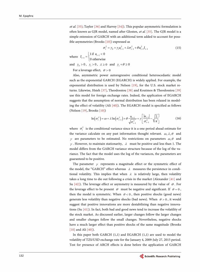
Figure 1 also shows that there are considerable ups and downs in the ex-change rate over the sample period. To see this more vividly, Figure 2 plots the changes in the logs of the daily exchange rate. The significant point to note from Figure 2 is that volatility occurs in clusters. There appears to have been a pro-longed period of relative tranquility in the market during the 300th - 400th days and during the 700th - 1400th days, evidenced by only relatively small positive and negative returns. On the other hand, during the 1st - 200th days, 400th - 700th days and 1400th - 1593rd days, there was far more volatility, when many large positive

M. Epaphra

124

Source: Author’s computations using data from Bank of Tanzania [24].

Figure 1. Log of TZS/USD daily exchange rate, 2009-2015.

Source: Author’s computations using data from Bank of Tanzania [24].

Figure 2. Change in log of TZS/USD daily exchange rate.

and large negative returns are observed during a short space of time. In essence, volatility is autocorrelated (Brooks [10]).

Figure 1 and Figure 2 provide evidence that time-varying volatility in daily TZS/USD returns is empirically shown as return clustering. The data show that TZS/USD exchange rate ranged from TZS 1280.30 on 4th Jan. 2009 to TZS 1601.17 on 22nd Feb. 2013. The TZS/USD exchange recorded the highest rates between TZS 1874.98 and TZS 2082.68 in the period between 4th May, 2015 and 27th July, 2015 (Bank of Tanzania, 2015). Low exchange rates were between TZS 1511 and TZS 1592 in the period spanning from 5th Dec. 2013 to 6th Jan. 2014 (Bank of Tanzania, 2015). This feature is referred to as the presence of ARCH/ GARCH effects (Humala & Rodríguez [14]).

The GARCH scheme developed in early 1980s is instrumental in popularizing

3.1

3.15

3.2

3.25

3.3

3.35

Log

Exch

ange

Rat

e (T

ZS/U

SD)

0 400 800 1200 1600Sample: 4 Jan. 2009 - 27 Jul. 2015

-.01

-.005

0.0

05.0

1

Cha

nge

in L

og E

xcha

nge

Rat

e (T

ZS/U

SD

)

0 400 800 1200 1600Sample: 4 Jan. 2009 - 27 Jul. 2015

M. Epaphra

125

this fact in economic modeling. By letting the conditional variance depend on the past squared innovations it directly captures the effect that once the market is heavily volatile it is more likely to remain so than to calm down and vice versa (de Vries & Leuven, [15]). Thus, GARCH models not only estimate the path for the time-varying conditional variance of the exchange rate, but also enable us to capture the appropriate conditional volatility present in the exchange rate (Chi-pili [16]).

Furthermore, downward movement of exchange rate (depreciation) is always followed by higher volatility. This characteristic that is exhibited by percentage changes in exchange rate is termed leverage effects (Abdalla [7] and Syarifuddin et al. [17]). In fact, price movements are negatively correlated with volatility (Abdalla [17]). Previous studies also show that volatility is higher after negative shocks than after positive shocks of the same magnitude (Black [18]). Black [18] attributes asymmetry to leverage effects. In this context, negative shocks increase predictable volatility in asset markets more than positive shocks. Empirical evi-dence on leverage effects also can be found in Nelson ([19]), Gallant et al. ([20] [21]), Campbell and Kyle ([22]) and Engle and Ng ([23]).

2.2. Non-Normality Distribution of Fat Tails

Stylized facts for financial returns usually suggest strong deviations from the normal distribution (Humala & Rodríguez [14]). The statistic proposed by Bera & Jarque [25] provides a formal assessment of how much the skewness and kur-tosis deviate from the normality assumptions of symmetry (zero skewness) and a .fixed peak of three. The Jarque-Bera (JB) test statistics is calculated as

( )22 3

6 4KTJB S

− =

(2)

where 3

1

1ˆ

Tt

t

x xS

T σ=

− =

∑ , is the sample skewness. This third moment or skew-

ness is an indicator of the asymmetry in the return distribution. 4

1

1ˆ

Tt

t

x xK

T σ=

− =

∑ , is the sample kurtosis. The fourth moment or kurtosis is a

measure of the peakness of the distribution. T is the sample size, x is the sam-ple mean and σ̂ is the estimated standard deviation. JB statistics follows chi-square ( )2χ distribution with two degrees of freedom for large sample. The null hypothesis in this test is that data follow normal distribution. The den-sity function for a normal distribution is given by

( )21 1exp

22πt

tx x

f xσσ

− = − (3)

The first assessment of the degree of departure from normality is to fit a Ker-nel distribution (smoothing the histogram) to the data and compare it with the normal distribution with mean and standard deviation based on the data sample effects (Humala & Rodríguez [14]). A kernel density provides an empirical esti-

M. Epaphra

126

mation of the density function of a random variable without parameterizing it theoretically (Humala & Rodríguez [14]). For the exchange rate, the kernel den-sity estimate is a function

( )1

1 Tt

t

x xf x W

Th h=

= =

∑ (4)

where T is the number of observations, h is the smoothing parameter or band-width and W is a kernel weighting function. Figure 3 reports, normality test, Kernel distribution, skewness and kurtosis using daily TZS/USD exchange rate data. The JB test rejects the null hypothesis of zero skewness and zero excess kurtosis at 5 percent level. This confirms departure from normality.

When the distribution of financial time series such as exchange rate returns is compared with the normal distribution, fatter tails are observed. A fat-tailed or thick-tailed distribution has a value for kurtosis that exceeds 3. That is, excess kurtosis is positive. This is called leptokurtosis. In other words, exchange rate returns irrespective of the regime when standardized by their scale exhibit more probability mass in the tails than distributions like the standard normal distribu-tion. This means that extremely high and low realizations occur more frequently than under the hypothesis of normality. The distinction between thin tailed dis-tributions like the normal distribution and fat tailed distributions is that the former have tails which decline exponentially fast while the latter distributions have tails which decline by a power (de Vries & Leuven [15]). In particular, Fig-ure 3 indicates that exchange rate series are not normally distributed and that the empirical distribution is more peaked than the normal density and it has fat-ter tails or excess kurtosis. Since the exchange rate return series exhibits depar-tures from normality, the volatility models are estimated with a student’s t dis-tribution framework.

JB = 24.13; Prob =0.00; Skewness = 0.20; Kurtosis = 3.55. Source: Author’s computations using data from Bank of Tanzania [24]

Figure 3. Normality test skewness and kurtosis of the daily TZS/USD.

010

2030

Den

sity

3.1 3.15 3.2 3.25 3.3 3.35Log Exchange Rate (TZS/USD)

M. Epaphra

127

2.3. Serial Correlation and Unit Root

Serial correlation renders inaccurate forecasts of financial returns as conven-tional risk estimates would be underestimated (Sheikh [26]). Serial correlation in financial asset returns is a form of non-normality and it appears whenever there is time dependence in the returns (Humala & Rodríguez [14]). The Ljung-Box Q-statistics is used to test for a null hypothesis of no serial correlation up to p lags. The Q-statistics is asymptotically distributed as a 2χ with degrees of free-dom equal to the number of autocorrelations being tested (Humala & Rodríguez [14]). If the corresponding p-value of the test is less than 0.05, the null of no serial correlation is rejected and, therefore, it can be concluded that there might be serial correlation in the returns (Humala and Rodríguez [14]). Figure 4 and Figure 5 plot the partial autocorrelogram and autocorrelogram (with 40 lags) of

H0: There is no serial correlation in the series; H1: There is serial correlation in the series. Source: Author’s computations using data from Bank of Tanzania [24]

Figure 4. Partial autocorrelation of exchange rate.

H0: There is no serial correlation in the series; H1: There is serial correlation in the series. Source: Author’s computations using data from Bank of Tanzania [24]

Figure 5. Autocorrelation of exchange rate.

-0.1

00.

000.

100.

20

Par

tial A

utoc

orre

latio

ns o

f Exc

hang

e R

ate

(TZS

/US

D)

0 10 20 30 40Lag

95% Confidence bands [se = 1/sqrt(n)]

-0.5

00.

000.

501.

00

Auto

corre

latio

ns o

f Log

Exc

hang

e R

ate

(TZS

/USD

)

0 10 20 30 40Lag

Bartlett's formula for MA(q) 95% confidence bands

M. Epaphra

128

the TZS/USD returns and the upper bound of the 95 per cent Bartlett’s confi-dence interval for the null hypothesis of no autocorrelation. These graphs illu-strate that exchange rates exhibit volatility clustering (that is, volatility shows positive autocorrelation) and the shocks to volatility take several months to die out. In addition, exchange rate exhibits autocorrelation at much longer horizons than one would expect.

The main feature of this correlogram is that the autocorrelation coefficients at various lags are very high even up to a lag of 40 quarters. This is the typical cor-relogram of a non-stationary series. The autocorrelation coefficient starts at a very high value and declines very slowly toward zero as the lag lengthens, also indicating presence of autocorrelation in the random walk series.

Furthermore, for high-frequency data like exchange tares, volatility is highly persistent (Long Memory) and there exists evidence of unit root behaviour of the conditional variance process (Longmore & Robinson [27]). The stylized fact here is that the logarithm of the nominal exchange rate for two freely floating currencies is non stationary, while the first difference is stationary1. The Aug-mented Dickey-Fuller (ADF) and Phillip-Perron (PP) methods are conducted to check for a unit root for the random walk series in both levels and first differ-ences.

Unit root test results are reported in Table 1, which indicate that the hypothe-sis of a unit root cannot be rejected in levels. It is therefore concluded that daily TZS/USD exchange rate is non-stationary in its levels. However, the hypothesis of a unit root is rejected in first differences. The unit root test results for the first difference are reported in Table 2. This also suggests that, further estimations

Table 1. ADF and PP unit root tests for stationarity in levels.

Unit Root Tests (in Level) Test Statistic 1% Critical Value 5% Critical Value

Dickey Fuller (DF) Z(t) −1.589 −3.430 −2.430

Phillips-Perron (PP) Z(t) −1.031 −3.430 −2.860

MacKinnon approximate value for Z(t) = 0.99

Source: Author’s computations using data from Bank of Tanzania [24].

Table 2. ADF and PP unit root tests for stationarity in first difference.

Unit Root Tests (1st Difference) Test Statistic 1% Critical Value 5% Critical Value

Dickey Fuller (DF) Z(t) −31.761 −3.430 −2.430

Phillips-Perron (PP) Z(t) −31.942 −3.430 −2.860

MacKinnon approximate value for Z(t) = 0.00

Source: Author’s computations using data from Bank of Tanzania [24].

1A stochastic process ( ){ }s t , where ( )s t is a random variable and t N∈ , is said to be stationary

if for any positive integer k and any points 1, , mt t the joint distribution of ( ) ( ){ }1 , , ms t t is the

same as the joint distribution of ( ) ( ){ }1 , , ms t k s t k+ + , that is the joint distribution is invariant

under time shift. A process ( ){ }s t is weakly or covariance stationary if ( ) ( )( )cov ,s m s k de-

pends only on the time difference m k− (de Vries and Leuven, 1994).

M. Epaphra

129

could be carried while in first difference in order to avoid spurious correlation. Characteristics of exchange rate series presented above suggest that a good

model for exchange rate series should capture serial correlation, time-varying variance, long-memory, peakedness as well as fat tails. The next section presents models that attempt to capture those features.

3. Parametric Volatility Models 3.1. The ARCH Model

Important features of series of financial time series data such as heteroscedasticity and volatility clustering provide a motivation for the application of ARCH model. Let 2

tσ denote the conditional variance of random variable, tu , that is2

( ) ( )( )221 2 1 2var , , , ,t t t t t t t tu u u E u E u u uσ − − − −

= = − (5)

Since ( ) 0tE u = , therefore

( )2 21 2 1 2var , , , ,t t t t t t tu u u E u u uσ − − − − = =

(6)

Equation (6) means that the conditional variance of random variable, tu , equals the conditional expected value of the square of tu . Under the ARCH model, the autocorrelation in volatility is modeled by allowing the conditional variance of the error term to depend on the immediately previous value of the squared error (Brooks [10]), that is

2 20 1 1t tuσ γ γ −= + (7)

Here, tu is normally distributed with zero mean and ( ) ( )20 1 1var t tu uγ γ −= +

i.e. ( )20 1 10,t tu N uγ γ −+

. 0γ and 1γ are unknown parameters. In other words, equation (7) states that the variance of the random variable tu follows an ARCH (1) process, since the conditional variance depends on only one lagged squared error3. Under ARCH, the equation which describes how the regressand

tr , varies over time (the mean equation) could take any form (Brooks [10]). For the purpose of this paper, full model is expressed as

t tr uµ= + , ( )2~ 0,t tu N σ

2 20 1 1t tuσ γ γ −= + (8)

and 0 0γ ≥ and 1 0γ ≥ Since 2

tσ is a conditional variance, its value must always be strictly positive. The error variance, however, may depend not only on one lagged squared error but also on several lagged squared errors. Therefore, model (8) can be extended to the general case where the error variance depends on p lags of squared er-ror

t tr uµ= + , ( )2~ 0,t tu N σ

2See Brooks (2008) for more details. 3The variance of u at time t is dependent on the squared error term at time 1t − , thus giving the appearance of heteroskedasticity or serial correlation.

M. Epaphra

130

2 20 1 1 2 2t t t p t pu u uσ γ γ γ γ− − −= + + + + (9)

and 0 0,1,2, ,i i pγ ≥ ∀ = The null hypothesis in this test is that there is no ARCH effect, while an alter-

native effect is that there is ARCH effect. If there is no serial correlation in the error variance, then

0 1 1: 0pH γ γ γ= = = = (10)

Since 2tσ cannot be easily observed, Gujarati & Porter [1] and Engle [4]

show that running the regression 2 2

0 1 1 2 2ˆ ˆ ˆ ˆˆ ˆ ˆ ˆt t t p t pu u u uγ γ γ γ− − −= + + + + (11)

can easly test the null hypothesis of no ARCH effect. The ARCH (1) is a special case of ARCH (q) and therefore what applies for ARCH (q) also applies for ARCH (1)

3.2. The GARCH Model

The Generalized ARCH (GARCH) is an extension of the ARCH model. When modeling using ARCH, there might be a need for a large value of the lag p, hence a large number of parameters. This may result in a model with a large number of parameters, violating the principle of parsimony and this can present difficulties when using the model to adequately describe the data. Also, the more parameters there are in the conditional variance equation, the more likely it is that one or more of them will have negative estimated value, violating the non- negativity constraints4. A GARCH model may contain fewer parameters as com- pared to an ARCH model, and thus a GARCH model may be preferred to an ARCH model.

Bollerslev [5] generalizes the simple ARCH model with the parsimonious. The GARCH model allows the conditional variance to be present upon previous lags. The GARCH (1,1) with mean equation can be expressed as

t tr uµ= + , ( )2~ 0,t tu N σ

2 2 20 1 1 1t t tuσ γ γ λσ− −= + + (12)

Model (12) states that the conditional variance of tu depends not only on the squared error in the previous time period but also on its conditional variance in the previous period. According to Brooks [10], using the GARCH model, it is possible to interpret the current fitted variance as a weighted function of a long-term average value, information about volatility during the previous period and the fitted variance from the model during the previous period. The GARCH (1,1) is the simplest and most robust of the family of volatility models (Engle [4]). However, the model can be extended to a GARCH (p,q) model where the current conditional variance is parameterized to depend upon p lagged terms of the squared error and q terms of the lagged conditional variance.

2 2 2 2 20 1 1 2 2 1 1 2 2t t t p t p t t q t qu u uσ γ γ γ γ λ σ λ σ λ σ− − − − − −= + + + + + + + + (13)

4See Brooks (2008) for more detail.

M. Epaphra

131

Also, the restrictions 0 1 2, , , , 0,pγ γ γ γ ≥ and 1 2, , , 0qλ λ λ ≥ are im-posed in order for the variance 2

tσ be positive. In general a GARCH (1,1) mod-el is sufficient to capture the volatility clustering in the data (Brooks [10]).

3.3. The ARCH-GARCH Estimation

Maximum likelihood technique is employed to estimate models from the ARCH family. Essentially, the method works by finding the most likely values of the parameters given the actual data. More specifically, a log-likelihood function is formed and the values of the parameters that maximize it are sought (Brooks [10]). In the form of conditional heteroscedasticity, the model for the mean and variance ( ) ( )AR 1 GARCH 1,1− can be expressed as

1t t tr r uµ ϕ −= + + , ( )2~ 0,t tu N σ

2 2 20 1 1 1t t tuσ γ γ λσ− −= + +

where the variance of the errors, 2tσ , is time-varying. Weiss [28], Bollerslev &

Wooldridge [29] and Brooks [10] specify the log-likelihood function (LLF) that maximize under the normality assumption for the disturbances as

( ) ( ) ( )22 21

1 1

1 1 1log 2π log2 2 2

T T

t t t tt t

L r rσ µ ϕ σ−= =

= − − − − −∑ ∑ (14)

where ( )1 log 2π2

− is a constant with respect to the parameters, T is the

number of observations and tr is exchange rate return. According to Brooks

[10], maximization of the LLF necessitates minimization of ( )2

1log

T

tt

σ=∑ ,

( )2 21

1

T

t t tt

r rµ ϕ σ−=

− −∑ and error variance. However, the normal distribution

cannot account for the pronounced fat tails of exchange rate returns. To account for this characteristic, fat tailed distribution, the Generalized Error distribution (GED) is widely applied (Erdemlioglu, et al. [3]; Palm [30]; Pagan [31]; Bollers-lev, et al. [32] and Brooks [10]).

3.4. The Leverage Effects and Asymmetric GARCH Model

As presented earlier, the leverage effect is the phenomenon of a correlation of past returns with future volatility. Volatility tends to increase when stock prices drop. When volatility rises, expected returns tend to increase, leading to a drop in the stock price. As a result, volatility and stock returns are negatively corre-lated. Also, when stock prices fall, financial leverage increases, leading to an in-crease in stock return volatility (Aydemir et al. [33] and Harvey [34]). Leverage effects enable the conditional variance of random variable, 2

tσ to respond asymmetrically to positive and negative values of tr . Unfortunately, GARCH models enforce a symmetric response of volatility to positive and negative shocks. Leverage effects are incorporated into GARCH models by including a variable in which the squared observations are multiplied by an indicator that takes a value of unity when observation is negative and zero otherwise (Glosten,

M. Epaphra

132

et al. [35]; Taylor [36] and Harvey [34]). This popular asymmetric formulation is often known as GJR model, named after Glosten, et al. [35]. The GJR model is a simple extension of GARCH with an additional term added to account for poss-ible asymmetries (Brooks [10]) expressed as

2 2 2 20 1 1 1 1 1t t t t tu u Iσ γ γ λσ θ− − − −= + + + (15)

where 11

1 if 00 otherwise

tt

uI −−

<=

and 0 0γ > , 1 0γ > , 0λ ≥ and 1 0γ θ+ ≥

For a leverage effect, 0θ > Also, asymmetric power autoregressive conditional heteroscedastic model

such as the exponential GARCH (EGARCH) is widely applied. For example, the exponential distribution is used by Nelson [19], for the U.S. stock market re-turns. Likewise, Hsieh [37], Theodossiou [38] and Koutmos & Theodossiou [39] use this model for foreign exchange rates. Indeed, the application of EGARCH suggests that the assumption of normal distribution has been relaxed in model-ing the effect of volatility (Ali [40]). The EGARCH model is specified as follows (Nelson [19], Brooks [10])

( ) ( ) 12 2 11 22

11

2ln lnπ

ttt t

tt

uuσ ω λ σ θ γ

σσ−−

−−−

= + + + −

(16)

where 2tσ is the conditional variance since it is a one period ahead estimate for

the variance calculate on any past information thought relevant. , ,ω λ θ and γ are parameters to be estimated. No restrictions on parameters ,ω θ and γ . However, to maintain stationarity, λ must be positive and less than 1. The model differs from the GARCH variance structure because of the log of the va-riance. The fact that the model uses the log of the variances, the parameters are guaranteed to be positive.

The parameter γ represents a magnitude effect or the symmetric effect of the model, the “GARCH” effect whereas λ measures the persistence in condi-tional volatility. This implies that when λ is relatively large, then volatility takes a long time to die out following a crisis in the market (Alexander [41] and Su [42]). The leverage effect or asymmetry is measured by the value of θ . For the leverage effect to be present θ must be negative and significant. If 0θ = , then the model is symmetric. When 0θ < , then positive shocks (good news) generate less volatility than negative shocks (bad news). When 0θ > , it would suggest that positive innovations are more destabilizing than negative innova-tions (Su [41]). In fact, both bad and good news tend to increase the volatility of the stock market. As discussed earlier, larger changes follow the larger changes and smaller changes follow the small changes. Nevertheless, negative shocks have a much larger effect than positive shocks of the same magnitude (Brooks [10] and Ali [40]).

In this paper both GARCH (1,1) and EGARCH (1,1) are used to model the volatility of TZS/USD exchange rate for the January 4, 2009-July 27, 2015 period. Test for presence of ARCH effects is done before the application of GARCH

M. Epaphra

133

models. The test for the presence of ARCH effect is performed by first applying the least squares (LS) method in order to generate regression residuals. Then the ARCH heteroskedasticity test is applied to the residuals to ascertain whether time varying volatility clustering does exist (Gujarati & Porter [1] and Brooks [10]).

4. Empirical Results 4.1. Volatility Clustering in Residuals

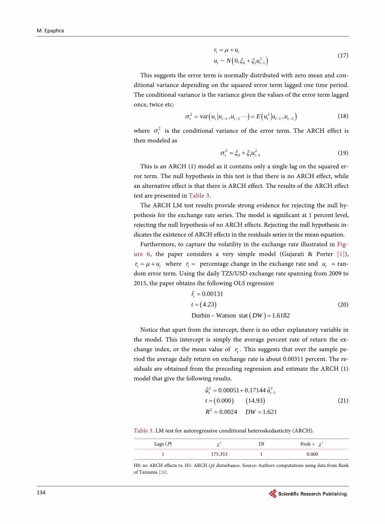
Before estimating the ARCH and GARCH models, the paper investigates the exchange rate series in order to identify its statistical properties and to see if it meets the pre-conditions for the ARCH and GARCH models, that is, clustering volatility and ARCH effect in the residuals. Figure 6 reports the results of the test of clustering volatility in the residuals or error term. The Figure shows that large and small errors occur in clusters, which imply that large returns are fol-lowed by more large returns and small returns are further followed by small re-turns. In other words, the Figure suggests that periods of high exchange rate are usually followed by further periods of high exchange rate, while low exchange rate is likely to be followed by much low exchange rate. This clustering volatility suggests that residual or error term is conditionally heteroscedastic and it can be estimated by ARCH and GARCH models.

4.2. Results of Heteroscedasticity Test: The ARCH Effect

The ARCH effect is concerned with a relationship within the heteroskedasticity, often termed serial correlation of the heteroskedasticity. It often becomes ap-parent when there is bunching in the variance or volatility of a particular varia-ble, producing a pattern which is determined by some factor. Given that the vo-latility of exchange rate is used to represent its risk, it can be argued that the ARCH effect is measuring the risk of a financial asset. Given the model:

GARCH (1,1). Source: Author’s computations using data from Bank of Tanzania [24].

Figure 6. Volatility clustering test: Residuals.

-.01

-.005

0.0

05.0

1

Res

idua

ls

0 400 800 1200 1600Sample: 4 Jan. 2009 - 27 Jul. 2015

M. Epaphra

134

( )20 1 1~ 0,

t t

t t

r u

u N u

µ

ξ ξ −

= +

+ (17)

This suggests the error term is normally distributed with zero mean and con-ditional variance depending on the squared error term lagged one time period. The conditional variance is the variance given the values of the error term lagged once, twice etc:

( ) ( )2 21 2 1 2var , ,t t t t t t tu u u E u u uσ − − − −= =

(18)

where 2tσ is the conditional variance of the error term. The ARCH effect is

then modeled as 2 2

0 1 1t tuσ ξ ξ −= + (19)

This is an ARCH (1) model as it contains only a single lag on the squared er-ror term. The null hypothesis in this test is that there is no ARCH effect, while an alternative effect is that there is ARCH effect. The results of the ARCH effect test are presented in Table 3.

The ARCH LM test results provide strong evidence for rejecting the null hy-pothesis for the exchange rate series. The model is significant at 1 percent level, rejecting the null hypothesis of no ARCH effects. Rejecting the null hypothesis in-dicates the existence of ARCH effects in the residuals series in the mean equation.

Furthermore, to capture the volatility in the exchange rate illustrated in Fig-ure 6, the paper considers a very simple model (Gujarati & Porter [1]),

t tr uµ= + where tr = percentage change in the exchange rate and tu = ran-dom error term. Using the daily TZS/USD exchange rate spanning from 2009 to 2015, the paper obtains the following OLS regression

( )( )

ˆ 0.001314.23

Durbin Watson stat 1.6182

trt

DW

=

=

− =

(20)

Notice that apart from the intercept, there is no other explanatory variable in the model. This intercept is simply the average percent rate of return the ex-change index, or the mean value of tr . This suggests that over the sample pe-riod the average daily return on exchange rate is about 0.00311 percent. The re-siduals are obtained from the preceding regression and estimate the ARCH (1) model that give the following results.

( ) ( )

2 21

2

ˆ ˆ0.00051 0.171440.000 14.93

0.0024 1.621

t tu ut

R DW

−= +

=

= =

(21)

Table 3. LM test for autoregressive conditional heteroskedasticity (ARCH).

Lags (P) 2χ Df Prob > 2χ

1 175.353 1 0.000

H0: no ARCH effects vs. H1: ARCH (p) disturbance. Source: Authors computations using data from Bank of Tanzania [24].

M. Epaphra

135

where ˆtu is the estimated residual from regression (20). Since the lagged squared error term is statistically significant, it suggests that the error variances are correlated, implying that there is an ARCH effect. The study tries higher- order ARCH models e.g. ARCH (5) and finds that coefficients on 2

2tu − , 23tu − ,

24−tu and 2

5tu − are all individually statistically significant at the 1 percent signi-ficance level (see Appendix A1). The fact, the return exhibits an ARCH effect, it is appropriate to apply GARCH model that is sufficient to cope with the chang-ing variance.

4.3. The GARCH (1,1) Estimation Results

Consistent with many previous studies (see for example, Franses & Van Dijk [43], Gokcan [44] and AL-Najjar [45], the study applies the GARCH (1,1). This GARCH (1,1) model of the daily percentage change in exchange rate, is esti-mated using data from January 4, 2009 through July 27, 2015, and the results as reported as follows

( ) ( ) ( )

2 2 21 1

2

ˆ ˆ0.0005 0.151 0.6030.059 5.055 11.491

0.001 1.622

t t tut

R DW

σ σ− −= + +

=

= =

(22)

The coefficients on both the lagged squared residual ( )21tu − and lagged con-

ditional variance ( )21tσ − terms in the conditional variance equation are indivi-

dually statistically significant at the 1 percent significance level. This suggests that volatility from the previous periods has a power of explaining the current volatility condition. One measure of the persistence of movements in the va-riance is the sum of the coefficients on 2

1tu − and 21tσ − in the GARCH model

(Stock & Watson [46]). The sum of 0.75 is large, indicating that changes in the conditional variance are persistence. In other words, a large sum of these coeffi-cients will imply that a large positive or a large negative return will lead future forecasts of the variance to be high for a protracted period. This implication is consistent with the long periods of volatility clustering reported in Figure 6. Like-wise, the GARCH (1,1) coefficients are positive confirming the non-negativity condition of the model.

4.4. The Leverage Effects and Asymmetric Results

In order to capture the availability of asymmetric behavior and the existence of leverage effect in the TZS/USD exchange rate, the paper applies EGARCH mod-el. As defined earlier, it is expected that the sign of θ in EGARCH model must be negative and significant. Regression Equation (23) reports the EGARCH re-sults.

( ) ( ) ( ) ( )

2 2 2 21 1 1 1

2

ˆ ˆ2.02 08 0.264 0.717 0.17630.57 22.50 137.50 6.86

0.002 1.717

t t t t tE u u It

R DW

σ σ− − − −= − + + −

= −

= =

(23)

All estimated parameters are statistically significant at 1 percent level of signi-ficance. Regarding the indicator for asymmetric volatility, estimates show that

M. Epaphra

136

the coefficient for the asymmetric volatility, θ , is negative, suggesting that posi-tive shocks imply a higher next period conditional variance than negative shocks of the same sign. This result is consistent with Brooks [10] for Japanese yen-US dollar returns data.

4.5. Diagnostic Checking of the GARCH (1,1) Model

Goodness of fit of the ARCH-GARCH model is based on residuals. The residuals are assumed to be independently and identically distributed following a normal or standardized t-distribution (Tsay [8] and Gourieroux [47]). If the model fits the data well the histogram of the residuals should be approximately symmetric. The ACF and the PACF of the standardized residuals are used for checking the adequacy of the conditional variance model. Having established that the model fits the data well, the fitted model can be used for forecasting.

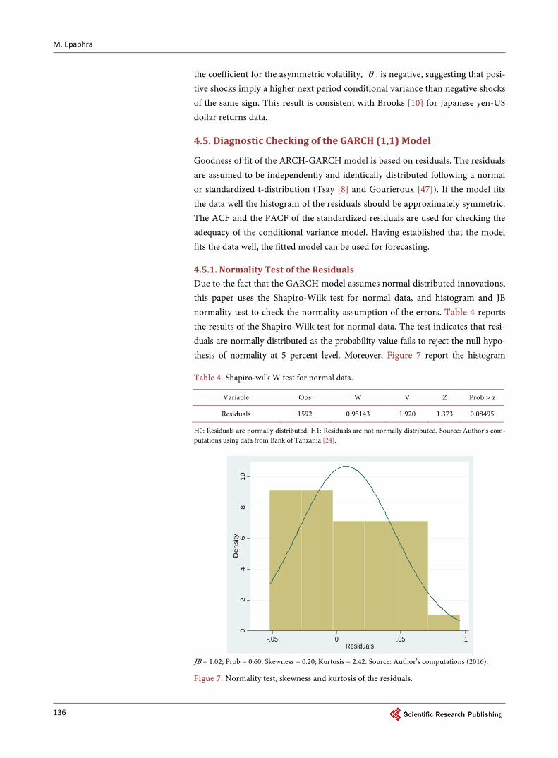
4.5.1. Normality Test of the Residuals Due to the fact that the GARCH model assumes normal distributed innovations, this paper uses the Shapiro-Wilk test for normal data, and histogram and JB normality test to check the normality assumption of the errors. Table 4 reports the results of the Shapiro-Wilk test for normal data. The test indicates that resi-duals are normally distributed as the probability value fails to reject the null hypo-thesis of normality at 5 percent level. Moreover, Figure 7 report the histogram

Table 4. Shapiro-wilk W test for normal data.

Variable Obs W V Z Prob > z

Residuals 1592 0.95143 1.920 1.373 0.08495

H0: Residuals are normally distributed; H1: Residuals are not normally distributed. Source: Author’s com-putations using data from Bank of Tanzania [24].

JB = 1.02; Prob = 0.60; Skewness = 0.20; Kurtosis = 2.42. Source: Author’s computations (2016).

Figue 7. Normality test, skewness and kurtosis of the residuals.

02

46

810

Den

sity

-.05 0 .05 .1Residuals

M. Epaphra

137

and skewness and kurtosis of the residuals of the fitted GARCH (1,1) respective-ly. Unsurprisingly, and as in the Shapiro-Wilk test for normal data, the normali-ty test indicates that residuals of the GARCH (1,1) model are normally distri-buted as we are unable to reject the null hypothesis of normality using Jac-que-Bera at 5 percent level.

4.5.2. Serial Correlation One simple diagnostic that is applied to know whether the model is a reasonable fit to the data is to obtain residuals and the AC and PAC of these residuals at any different lags. The estimated AC and PAC are shown in Figure 8 and Figure 9. As the figures show, none of the autocorrelations and partial correlations are

H0: There is no serial correlation in the residuals; H1: There is serial correlation in the residuals. Source: Author’s computations using data from Bank of Tanzania [24].

Figure 8. Autocorrelation of residuals.

H0: There is no serial correlation in the residuals; H1: There is serial correlation in the residuals. Source: Author’s computations using data from Bank of Tanzania [24].

Figure 9. Partial autocorrelation of residuals.

-0.4

0-0

.20

0.00

0.20

0.40

Auto

corre

latio

ns o

f Res

idua

ls

0 10 20 30 40Lag

Bartlett's formula for MA(q) 95% confidence bands

-0.4

0-0

.20

0.00

0.20

0.40

Parti

al A

ucor

rela

tions

of R

esid

uals

0 5 10 15Lag

95% Confidence bands [se = 1/sqrt(n)]

M. Epaphra

138

Table 5. Serial correlation test.

Lag AC PAC Q-Stat Prob. 3 −0.065 −0.062 0.3376 0.953 6 −0.101 −0.108 0.8820 0.990 9 −0.043 −0.017 4.2496 0.894

12 −0.049 −0.144 6.4183 0.894 15 −0.111 −0.063 8.0495 0.922 18 −0.042 −0.194 9.0030 0.960

H0: There is no serial correlation in the residuals. Source: Author’s computations using data from Bank of Tanzania [24].

individually statistically significant at 5 percent level. Likewise, in the post esti-mation analysis using standardized innovations based on the estimated model, the test for serial correlation using Correlogram presented in Table 5 indicates that there is no serial correlation in the model since none of the lag is found to be significant at 5 percent level, confirming the explanatory power of the GARCH (1,1) model. Moreover, the test shows that no any ARCH effects left (i.e. no heteroscedasticity). Thus, the model can be used to forecast future values of the exchange rate series.

4.6. Forecasting Evaluation and Accuracy

Forecasting provides basis for economic and business planning, inventory and production control and optimization of industrial process (Box & Jenkins [48]). Various measures of forecasting errors namely mean absolute error (MAE); the root mean squared error (RMSE); and Thieles’s U for the GARCH (1,1) are ap-plied in this paper. MAE and RMSE are computed as follows

2 2

1

1 ˆMAET

t tt

rT

σ=

= −∑ (24)

( )2

2 2

1

1 ˆRMAET

t tt

rT

σ=

= −∑ (25)

where 2ˆtσ for 1, ,t T= is the estimated conditional variance obtained from fitting ARCH-GARCH model. 2

tr is used as a substitute for the realized or ac-tual variance (Hung-Chung, et al. [49] and Franses & Dijk [43]). These two symmetric statistical loss functions are among the most popular methods for evaluating the forecasting power of a model given their simple mathematical forms (Vee & Gonpot [50]). The RMSE assigns greater weight to large forecast errors. This fact is dealt with using the MAE which on the contrary assigns equal weights to both over and under predictions of volatility. The smaller the error the better the forecasting ability of that model accordingly.

Another forecast method which is popular is Theil’s U-statistic. The Theil’s U test which is used to test accuracy of the future forecasts/predictions is defined as

( )

( )

11 22

1 11

1 21

1

FPE APE

APE

T

t tt

T

tt

U

−

+ +=

−

+=

− =

∑

∑ (26)

M. Epaphra

139

where ( )1

1

ˆFPE

t tt

t

X X

X+

+

−= is the forecast relative change, and

( )11APE t t

tt

X XX

++

−= is the actual relative change (Diebold & Lopez [51]). This

statistic is scale invariant. The Theil inequality coefficient always lies between zero and one, where zero indicates a perfect fit. That in turn occurs only when the forecasts are exact or give 0 errors.

Table 6 reports the MAE, RMSE and Theil’s U-statistic for the forecast vola-tility. The table shows that the GARCH (1,1) model seems to produce relatively accurate forecasts given the quite low MAE and RMSE values. Specifically, the lower MAE and RMSE scores produced by the GARCH (1,1) indicate that the model has better forecasting power. Likewise, the Theil’s statistic of 0.889 is less than one which indicates that the forecasts are fairly accurate.

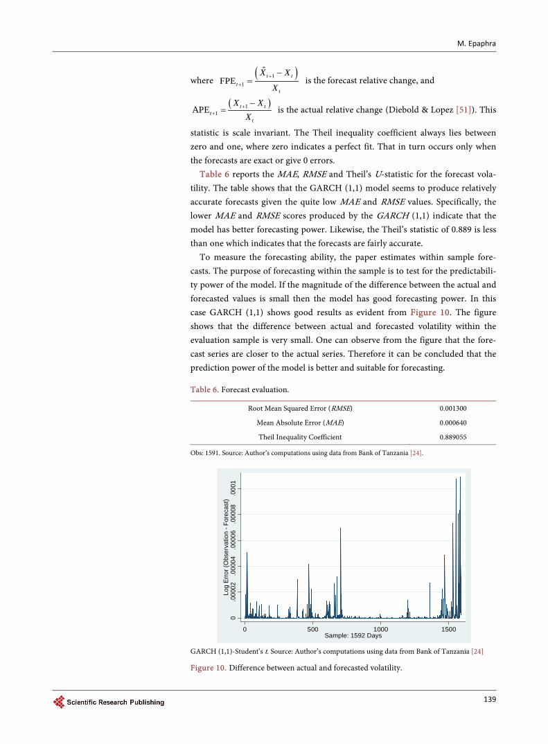
To measure the forecasting ability, the paper estimates within sample fore-casts. The purpose of forecasting within the sample is to test for the predictabili-ty power of the model. If the magnitude of the difference between the actual and forecasted values is small then the model has good forecasting power. In this case GARCH (1,1) shows good results as evident from Figure 10. The figure shows that the difference between actual and forecasted volatility within the evaluation sample is very small. One can observe from the figure that the fore-cast series are closer to the actual series. Therefore it can be concluded that the prediction power of the model is better and suitable for forecasting.

Table 6. Forecast evaluation.

Root Mean Squared Error (RMSE) 0.001300

Mean Absolute Error (MAE) 0.000640

Theil Inequality Coefficient 0.889055

Obs: 1591. Source: Author’s computations using data from Bank of Tanzania [24].

GARCH (1,1)-Student’s t. Source: Author’s computations using data from Bank of Tanzania [24]

Figure 10. Difference between actual and forecasted volatility.

0.0

0002

.000

04.0

0006

.000

08.0

001

Log

Erro

r (O

bser

vatio

n - F

orec

ast)

0 500 1000 1500Sample: 1592 Days

M. Epaphra

140

5. Conclusion

The accurate measurement and forecasting of the volatility of financial markets is crucial for the economy of Tanzania due to the fact that the country depends significantly on imports and that important reserves are held in foreign ex-change, especially in USD Moreover, there is an increasing amount of foreign investment in Tanzania. This paper aims at examining the volatility of exchange rate in Tanzania. To achieve this goal the empirical analysis involves ARCH/ GARCH models, so that to investigate the major volatility characteristics ac-companied with exchange volatility. In the same vein, the paper applies an EGARCH model to capture the asymmetry in volatility clustering and the leve-rage effect in exchange rate for the period spanning from January 4, 2009 to July 27, 2015. The empirical results suggest that the conditional variance or volatility is quite persistent for TZS/USD returns. In particular, the results show that ex-change rate behaviour in Tanzania is generally influenced by previous informa-tion about exchange rate. In other words, results suggest existence of conditional heteroscedasticity or volatility clustering. In this case, the paper concludes that the exchange rates volatility can be adequately modeled by the GARCH (1,1) model. The results of the Mean Absolute Error (MAE) and the Root Mean Square Error (RMSE) for the forecasted volatility show that GARCH (1,1) has a predictive power. However, the fact that GARCH (1,1) is symmetric, an asym-metric model, EGARCH estimation results suggest the presence of leverage ef-fect in the exchange rate volatility. The policy implication of these results is that, the fact that exchange rate forecasting is very important to gauge the benefits and cost of international trade, policy makers should be aware of the possible ef-fect of asymmetry when modeling volatility of an exchange rate series. In fact, there are plenty of practical applications of the results of this paper. Future re-search includes macroeconomic effect of exchange rate volatility in developing countries such as Tanzania. Variables such as interest rate, international re-serves, trade flows and openness may be considered.

References [1] Gujarati, N.D. and Porter, D.C. (2009) Basic Econometrics. International Edition

McGraw-Hill/Irwin, A Business Unit of The McGraw-Hill Companies, Inc., New York.

[2] Héricourt, J. and Poncet, S. (2012) Exchange Rate Volatility, Financial Constraints and Trade: Empirical Evidence from Chinese Firms. CEPII Discussion Paper.

[3] Erdemlioglu, D., Laurent, S. and Neely, C.J. (2012) Econometric Modeling of Ex-change Rate Volatility and Jumps. Working Paper Series, Research Division Federal Reserve Bank, St. Louis.

[4] Engle, R.F. (1982) Autoregressive Conditional Heteroscedasticity with Estimates of the Variance of UK Inflation. Econometrica, 50, 987-1007. https://doi.org/10.2307/1912773

[5] Bollerslev, T. (1986) Generalized Autoregressive Conditional Heteroskedasticity. Journal of Econometrics, 36, 394-419. https://doi.org/10.1016/0304-4076(86)90063-1

M. Epaphra

141

[6] Taylor, S.J. (1986) Modelling Financial Time Series. John Wiley and Sons, Ltd., Chichester.

[7] Abdalla, S.Z.S. (2012) Modeling Exchange Rate Volatility Using GARCH Models: Empirical Evidence from Arab Countries. International Journal of Economics and Finance, 4, 216-229. https://doi.org/10.5539/ijef.v4n3p216

[8] Tsay, R.S. (2002) Analysis of Financial Time Series. John Wiley and Sons, New York. https://doi.org/10.1002/0471264105

[9] Poon, S. (2005) A Practical Guide to Forecasting Financial Market Volatility. John Wiley Sons Inc., Hoboken.

[10] Brooks, C. (2008) Introductory Econometrics for Finance. 2nd Edition, Cambridge University Press, New York. https://doi.org/10.1017/CBO9780511841644

[11] Meese, R.A. and Rogoff, K. (1983) The Out-of-Sample Failure of Empirical Ex-change Rate Models: Sampling Error or Misspecification. In: Frenkel, J.A., Ed., Ex-change Rates and International Macroeconomics, University of Chicago Press, Chi-cago.

[12] Dornbusch, R. (1976) Expectations and Exchange Rate Dynamics. Journal of Politi-cal Economy, 84, 1161-1176. https://doi.org/10.1086/260506

[13] Branson, W.H., Halttunen, H. and Masson, P. (1979) Exchange Rates in the Short Run: Some Further Results. European Economic Review, 12, 395-402. https://doi.org/10.1016/0014-2921(79)90029-1

[14] Humala, A. and Rodríguez, G. (2010) Some Stylized Facts of Returns in the Foreign Exchange and Stock Markets. Peru. Serie de Documentos de Trabajo Working Pa-per Series.

[15] De Vries, G.C. and Leuve, K.U. (1994) Stylized Facts of Nominal Exchange Rate Returns. Purdue CIBER Working Papers.

[16] Chipili, J.M. (2012) Modeling Exchange Rate Volatility in Zambia. The African Finance Journal, 14, 85-107. http://hdl.handle.net/10520/EJC126376

[17] Syarifuddin, F., Achsani, N.A., Hakim, D.B. and Bakhtiar, T. (2014) Monetary Poli-cy Response on Exchange Rate Volatility in Indonesia. Journal of Contemporary Economic and Business Issues, 1, 35-54.

[18] Black, F. (1976) Studies of Stock Price Volatility Changes. In: Proceedings of the 1976 Meeting of the Business and Economic Statistics Section, American Statistical Association, Washington DC, 177-181.

[19] Nelson, D.B. (1991) Conditional Heteroskedasticity in Asset Returns: A New Ap-proach. Econometrica, 59, 347-370. https://doi.org/10.2307/2938260

[20] Gallant, A.R., Rossi, P.E. and Tauchen, G. (1993) Nonlinear Dynamic Structures. Econometrica, 61, 871-907. https://doi.org/10.2307/2951766

[21] Gallant, A.R., Rossi, P.E. and Tauchen G. (1992) Stock Prices and Volume. Review of Financial Studies, 5, 199-242. https://doi.org/10.1093/rfs/5.2.199

[22] Campbell, J.Y. and Kyle, A.S. (1993) Smart Money, Noise Trading and Stock Price Behaviour. Review of Economic Studies, 60, 1-34. https://doi.org/10.2307/2297810

[23] Engle, R.F. and Ng, V.K. (1993) Measuring and Testing the Impact of News on Vo-latility. Journal of Finance, 48, 1749-1778. https://doi.org/10.1111/j.1540-6261.1993.tb05127.x

[24] Bank of Tanzania (2015) www.bot.go.tz/

[25] Bera, A.K. and Jarque, C.M. (1982) Model Specification Tests: A Simultaneous Ap-proach. Journal of Econometrics, 20, 59-82. https://doi.org/10.1016/0304-4076(82)90103-8

M. Epaphra

142

[26] Sheikh, A.Z. and Qiao, H. (2010) Non-Normality of Market Returns: A Framework for Asset allocation Decision-Making. The Journal of Alternative Investments, Winter, 12, 8-35. https://doi.org/10.3905/JAI.2010.12.3.008

[27] Longmore, R. and Robinson, W. (2004) Modelling and Forecasting Exchange Rate Dynamics: An Application of Asymmetric Volatility Models. Working Paper, WP2004/03, Bank of Jamaica, Kingston.

[28] Weiss, A.A. (1986) Asymptotic Theory for ARCH Models: Estimation and Testing. Econometric Theory, 2, 107-131. https://doi.org/10.1017/S0266466600011397

[29] Bollerslev, T. and Woodridge, J.M. (1992) Quasi-Maximum Likelihood Estimation and Inference in Dynamic Models with Time-Varying Covariances. Econometric Review, 11, 143-172. https://doi.org/10.1080/07474939208800229

[30] Palm, F.C. (1996) GARCH Models of Volatility. In: Maddala, G. and Rao, C., Eds., Handbook of Statistics, Elsevier Science, Amsterdam, 209-240.

[31] Pagan, A. (1996) The Econometrics of Financial Markets. Journal of Empirical Finance, 3, 15-102. https://doi.org/10.1016/0927-5398(95)00020-8

[32] Bollerslev, T., Chou, R.Y. and Kroner, K.F. (1992) ARCH Modeling in Finance: A Selective Review of the Theory and Empirical Evidence. Journal of Econometrics, 52, 5-59. https://doi.org/10.1016/0304-4076(92)90064-X

[33] Aydemir, A.C., Gallmeyer, M. and Hollifield, B. (2007) Financial Leverage and the Leverage Effect—A Market and Firm Analysis. Paper 142, Tepper School of Busi-ness, Pittsburgh. http://repository.cmu.edu/tepper/142

[34] Harvey, A.C. (2013) Dynamic Models for Volatility and Heavy Tails: With Applica-tions to Financial and Economic Time Series. Econometric Society Monograph, Cambridge University Press, Cambridge. https://doi.org/10.1017/CBO9781139540933

[35] Glosten, L.R., Jagannathan, R. and Runkle, D.E. (1993) On the Relation between the Expected Value and the Volatility of the Nominal Excess Return on Stocks. Journal of Finance, 48, 1779-1801. https://doi.org/10.1111/j.1540-6261.1993.tb05128.x

[36] Taylor, S. (2005) Asset Price Dynamics, Volatility, and Prediction. Princeton Uni-versity Press, Princeton.

[37] Hsieh, D. (1989) Modeling Heteroscedasticity in Daily Exchange Rates. Journal of Business and Economic Statistics, 7, 307-317. https://doi.org/10.1080/07350015.1989.10509740

[38] Theodossiou, P. (1994) The Stochastic Properties of Major Canadian Exchange Rates. The Financial Review, 29, 193-221. https://doi.org/10.1111/j.1540-6288.1994.tb00818.x

[39] Koutmos, G. and Theodossiou, P. (1994) Time-Series Properties and Predictability of Greek Exchange Rates. Managerial and Decision Economics, 15, 159-167. https://doi.org/10.1002/mde.4090150208

[40] Ali, G. (2013) EGARCH, GJR-GARCH, TGARCH, AVGARCH, NGARCH, IGARCH and APARCH Models for Pathogens at Marine Recreational Sites. Journal of Statistical and Econometric Methods, 2, 57-73.

[41] Alexander, C. (2009) Market Risk Analysis, Value at Risk Models. Vol. 4, John Wi-ley and Sons, Hoboken.

[42] Su, C. (2010) Application of EGARCH Model to Estimate Financial Volatility of Daily Returns: The Empirical Case of China. Master Degree Project No. 2010: 142, University of Gothenburg, Gothenburg.

[43] Franses, P.H. and Dijk, D.V. (1996) Forecasting Stock Market Volatility Using

M. Epaphra

143

(Non-Linear) GARCH Models. Journal of Forecasting, 15, 229-235. https://doi.org/10.1002/(SICI)1099-131X(199604)15:3<229::AID-FOR620>3.0.CO;2-3

[44] Gokcan, S. (2000) Forecasting Volatility of Emerging Stock Market: Linear versus Non-Linear GARCH Models. Journal of Forecasting, 19, 499-504. https://doi.org/10.1002/1099-131X(200011)19:6<499::AID-FOR745>3.0.CO;2-P

[45] AL-Najjar, D.M. (2016) Modelling and Estimation of Volatility Using ARCH/GARCH Models in Jordan’s Stock Market. Asian Journal of Finance and Accounting, 8, 152-167. https://doi.org/10.5296/ajfa.v8i1.9129

[46] Stock, J.H. and Watson, M.W. (2007) Why Has U.S. Inflation Become Harder to Forecast? Journal of Money, Credit and Banking, 39, 3-33. https://doi.org/10.1111/j.1538-4616.2007.00014.x

[47] Gourieroux, C. (2001) Financial Econometrics, Problems, Models and Methods. Princeton Series in Finance, Princeton University Press, Princeton.

[48] Box, G.E.P. and Jenkins, G.M. (1976) Time Series Analysis: Forecasting and Con-trol. Revised Edition, Holden Day, San Francisco.

[49] Hung-Chung, L., Yen-Hsien, L. and Ming-Chih, L. (2009) Forecasting China Stock Markets Volatility via GARCH Models under Skewed-GED Distribution. Journal of Money, Investment and Banking, 7, 542-547.

[50] Vee, D., Ng, C., Gonpot, P.N. and Sookia, N. (2011) Forecasting Volatility of USD/MUR Exchange Rate Using a GARCH (1,1) Model with GED and Student’s-t Errors. University of Mauritius Research Journal, 17, 1-14.

[51] Diebold, F.X. and Lopez, J.A. (1995) Modeling Volatility Dynamics. In: Hoover, K., Ed., Macroeconometrics: Developments, Tensions and Prospects, Kluwer Academic Press, Boston, 427-466. https://doi.org/10.1007/978-94-011-0669-6_11

Appendix A1: ARCH (5) Variable Coefficient Std. Error z-Statistic Prob.

C −0.000951 0.000666 −1.427629 0.1534

Variance Equation

C 0.000799 3.62E−05 22.07692 0.0000

Resid(−1)2 1.066442 0.026461 40.30274 0.0000

Resid(−2)2 0.756990 0.030206 25.06066 0.0000

Resid(−3)2 0.414354 0.031467 13.16783 0.0000

Resid(−4)2 0.142838 0.014272 10.00827 0.0000

Resid(−5)2 0.130278 0.015494 8.408385 0.0000

R-squared 0.011992

Adjusted R-squared 0.011992

Durbin-Watson stat 1.589174

Source: Author’s computations using data from Bank of Tanzania [24].

Submit or recommend next manuscript to SCIRP and we will provide best service for you:

Accepting pre-submission inquiries through Email, Facebook, LinkedIn, Twitter, etc. A wide selection of journals (inclusive of 9 subjects, more than 200 journals) Providing 24-hour high-quality service User-friendly online submission system Fair and swift peer-review system Efficient typesetting and proofreading procedure Display of the result of downloads and visits, as well as the number of cited articles Maximum dissemination of your research work

Submit your manuscript at: http://papersubmission.scirp.org/ Or contact jmf@scirp.org