Embed Size (px)
Citation preview

arX
iv:2
010.
1485
6v1
[ec
on.E
M]
28
Oct
202
0
Modeling European regional FDI flows using a Bayesian
spatial Poisson interaction model
Tamás Krisztin∗1 and Philipp Piribauer2
1International Institute for Applied Systems Analysis (IIASA)2Austrian Institute of Economic Research (WIFO)
Abstract
This paper presents an empirical study of spatial origin and destination effects of European
regional FDI dyads. Recent regional studies primarily focus on locational determinants, but
ignore bilateral origin- and intervening factors, as well as associated spatial dependence.
This paper fills this gap by using observations on interregional FDI flows within a spatially
augmented Poisson interaction model. We explicitly distinguish FDI activities between three
different stages of the value chain. Our results provide important insights on drivers of regional
FDI activities, both from origin and destination perspectives. We moreover show that spatial
dependence plays a key role in both dimensions.
Keywords: Spatial interaction model, Bayesian Poisson model, regional FDI flows, Euro-
pean regions, spatial random effects.
JEL Codes: C11, C21, F23, R11
∗Corresponding author: Tamás Krisztin, International Institute for Applied Systems Analysis (IIASA), Schlossplatz1, 2361 Laxenburg, Austria. E-mail: [email protected]. The research carried out in this paper was supported byfunds of the Oesterreichische Nationalbank (Jubilaeumsfond project number: 18116), and of the Austrian Science Fund(FWF): ZK 35
1
1 Introduction
Recent decades have shown a rapid growth of worldwide foreign direct investment (FDI), which
led to increased efforts in research to understand the economic determinants of FDI activities.
Classical explanations focus on the factors driving firms to become multinational. The Ownership-
Localization-Internalization theory (see Dunning 2001) explains firms’ motivation as an effort to
internalize transaction costs and reap the benefits of externalities stemming from strategic assets.
A large alternative strand of empirical literature builds on trade theory. In this context the drivers
of FDI activity are the need for larger sales markets, cheaper source markets, and the willingness
to reach a technological frontier (Markusen 1995). Following empirical international economics
literature, FDI flows are usually captured within the context of a bilateral spatial interaction model
framework. The main advantage of this approach is that it specifically accounts for the role of
origin- and destination-specific factors, as well as intervening opportunities. For an overview on
the determinants of FDI activities and the location choice of multinationals, see Basile and Kayam
(2015), Blonigen and Piger (2014), or Blonigen (2005).
Due to the scarcity of data on FDI activities on a subnational scale, the vast majority of the
empirical literature focuses on country-specific FDI patterns. A subnational perspective, how-
ever, would allow for in-depth decomposition of the spatial patterns of FDI flows, since FDI
sources and destinations are not uniformly distributed within a country, but tend to be spatially
clustered. Multiple studies focusing on regional investment decisions of multinational companies
(Crescenzi et al., 2013; Ascani et al., 2016a) emphasize within-country heterogeneity of FDI de-
cisions, which can exceed cross-country differences. However, a major gap in the literature is that
regional level studies only focus on the destination of FDI decisions, and largely neglect to account
for origin-specific factors, as well as intervening opportunities in a subnational context. However,
a simultaneous treatment appears particularly important for providing a complete picture on third-
regional spatial interrelationships in both source- as well as destination-specific characteristics
(Leibrecht and Riedl, 2014). Moreover, neglecting to take into account both origin, destination,
and third region effects, can lead to biased parameter estimates (Baltagi et al., 2007).
The present paper aims to fill these gaps by focusing on subnational FDI flows in a European
multi-regional framework and explicitly accounting for origin-, destination-, as well as third region-
specific factors. In this paper we make use of subnational data from the fDi Markets database, which
reports on bilateral FDI flows, with detailed information on the source and destination city. This
can be compiled to multiple dyadic format, that is each region pair appears twice, corresponding to
FDI flowing from one region to the other and vice versa. A specific virtue of the database is that it
distinguishes FDI flows by their respective business activity. This allows us to contrast the impact
of origin, destination, and third region effects across multiple stages of the global values chain.
When adopting a subnational perspective, it is crucial to control for spatial dependence, as its
presence in regional data is well documented (LeSage and Pace, 2009). Even national-level empiri-
cal applications clearly document the presence of spatial spillovers on FDI activities. An influential
example is the work by Blonigen et al. (2007), who analyse the determinants of US outbound FDI
activities in a cross-country framework, while explicitly accounting for spatial dependence among
2
destinations. Further studies which document the presence of spatial issues amongst bilateral (na-
tional) FDI activities include Pintar et al. (2016), Regelink and Elhorst (2015), Chou et al. (2011),
Garretsen and Peeters (2009), Poelhekke and van der Ploeg (2009), or Baltagi et al. (2007).
We therefore employ an econometric framework in the spirit of Koch and LeSage (2015) and
LeSage et al. (2007) which captures not only third-regional effects but also spatial dependence using
spatially-augmented random effects. Estimation is achieved using work by Frühwirth-Schnatter et al.
(2009), allowing us to deal with the high-dimensional specifications in a flexible and computation-
ally efficient way.
The remainder of the paper is organized as follows. Section 2 presents the proposed spatial
interaction model, which is augmented by spatial autoregressive origin- and destination-specific
random effects, intended to capture spatially dependencies, as well as so-called third region effects.
Section 3 details the FDI data, the considered determinants, as well as our selection of regions. In
Section 4 we assess the determinants of European interregional FDI flows across different stages
of the global value chain. The analysis is performed using information on FDI dyads covering 266
NUTS-2 regions in the period 2003 to 2011. Section 5 concludes.
2 A spatial interaction model for subnational FDI flows
This section presents the model specification used for the empirical analysis. It is worth noting
that the spatial econometric model is similar to work by LeSage et al. (2007), who aimed at
modelling regional knowledge spillovers in Europe. An efficient Bayesian estimation approach for
the employed multiplicative form of the Poisson model with spatial random effects is provided in
the Appendix.1
Let y denote an # × 1 vector containing information on the number of FDI flows between
= regions.2 In the classic spatial interaction model framework the flows are regressed on corre-
spondingly stacked origin-, destination-, and distance-specific explanatory variables, as well as
their spatially lagged counterparts. ^> and ^3 denote # × ?- origin- and destination-specific
matrices of explanatory variables, respectively. Distances and further intervening factors between
the = regions are captured by the # × ?� matrix J.3 Extending the standard model specification
with local spillover effects as well as spatial random effects, we consider a Poisson specification of
the form:
y ∼ P(,)
, = exp(
U0 + ^>#> + ^3#3 + J$� +]>^>%> +]3^3%3 +\>)> + \3)3)
, (2.1)
1Detailed R codes for running the proposed model are available upon request.2It is worth noting that in the present study # is of lower dimension than =2, since FDI dyads by construction exhibit
no own-regional and no own-country flows.3Detailed information on the straightforward construction of the origin- and destination-specific matrices of explana-
tory variables ^> and ^3 from an = × ?- dimensional matrix of explanatory variables is provided in LeSage and Pace(2009). LeSage and Pace (2009) also provide detailed guidelines on the convenient construction of origin- anddestination-specific spatial weight matrices.
3

where P(·) denotes the Poisson distribution and U0 is an intercept parameter. #>, #3, and $� are
parameter vectors corresponding to ^>, ^3, and J, respectively. The spatial lags of the covariates
are captured by ]>^> and ]3^3, with %> and %3 denoting the respective ?- × 1 vectors of
parameters. Through these spatial lags we explicitly capture the so-called third region effects
(Baltagi et al., 2007), that is origin- and destination-specific spillovers from neighbouring regions.
Neighbourhood effects are governed by non-negative, row-stochastic spatial weight matrices, which
contain information on the spatial connectivity between the regions under scrutiny. Our Poisson
spatial interaction model includes separate spatial weight matrices ]> and ]3 to account for
origin- and destination-specific third regional effects, respectively.
Origin-based random effects are captured by the term\>)>, where\> denotes an # ×=matrix
of origin-specific dummy variables with a corresponding =×1 vector )>. Similarly, the =×1 vector
)3 captures regional effects associated with the destination regions’ matrix of dummy variables
\3 . We follow work by LeSage et al. (2007) and introduce a further source of spatial dependence
via the = × 1 regional effect vectors )> and )3, which are assumed to follow a first-order spatial
autoregressive process:
)> = d>])> + .> .> = N(
0, q2> O=
)
(2.2)
)3 = d3])3 + .3 .3 = N(
0, q23 O=
)
, (2.3)
where d> and d3 denote origin- and destination-specific spatial autoregressive (scalar) parameters,
respectively. ] denotes an = × = row-stochastic spatial weight matrix with known constants and
zeros on the main diagonal.
The disturbance error vectors .> and .3 are both assumed to be independently and identically
normally distributed, with zero mean and q2> and q2
3variance, respectively. Note that this assump-
tion implies a one-to-one mapping to origin- and destination-specific normally distributed random
effects in the case of d> = 0 and d3 = 0. For a row-stochastic ] , a sufficient stability condition
may be employed by assuming the spatial autoregressive parameters d> and d3 to lie in the interval
−1 < d>, d3 < 1 (see, for example, LeSage and Pace 2009).
3 Bilateral FDI data and regions
Our data set comprises observations on regional FDI dyads for 266 European NUTS-2 regions in
the period 2003 to 2011. A complete list of the regions in our sample is provided in Table A2 in
the Appendix.
Observations on regional cross-border greenfield FDI investments stem from the fDi Markets
database. This database is maintained by fDi Intelligence, which is a specialist division of the
Financial Times Ltd. The provided data draws on media and corporate sources to report on the
sources and hosts of FDI flows (detailed by country, region, and city), industry classifications, as
well as the level of capital investment. Crescenzi et al. (2013) report several robustness tests and
detailed comparisons with official data sources. They confirm the reliability of the fDi Markets
data set, especially with regard to the reported spatial distribution of FDI investments.
4

Our dependent variables are based on the total amount of inflows from European regions in
the period 2003 to 2011. Since the fDi Markets data base also contains information on several
distinct business activities for both origin and host companies, we follow previous studies by
Ascani et al. (2016a) and study the determinants of regional FDI dyads at different stages of
the value chain. This information is valuable as investor companies maximize their utility with
respect to their position along the value chain. Since specifics of the investor company, as well as
details on the FDI investment are largely unobserved, it is crucial to account for the heterogeneity
in investor decisions by subdividing industry activities relative to their position along the value
chain (see, for example, Ascani et al. 2016a). We therefore define three different classifications:
Upstream, Downstream, and Production. The classification adopted in this paper builds on general
classifications of the value chain by Sturgeon (2008) and closely tracks the ones employed by
Crescenzi et al. (2013) and Ascani et al. (2016a).
Specifically, the upstream category comprises conceptual product development including de-
sign and testing, as well as management and business administration activities. The downstream
category summarizes consumer-related activities such as sales, product delivery, or support. Fi-
nally, the production category includes activities related to physical product creation, including
extraction, manufacturing, as well as recycling activities. A complete list of the employed global
value chain classification is provided in Table A1 in the Appendix.
Our choices for explanatory variables are motivated by recent literature on (regional) FDI flows
as well as regional growth empirics (see, for example, Crespo Cuaresma et al. 2018, Blonigen and Piger
2014, Leibrecht and Riedl 2014, or Blonigen 2005). In most gravity-type models a region’s ability
to emit and attract FDI flows is chiefly captured by its economic characteristics. Our main indicator
for economic characteristics is the regions’ market size, proxied by regional gross value added.
To control for the degree of urbanization both in origin and host regions we also include regional
population densities as an additional covariate. Empirical evidence suggests (Coughlin et al., 1991;
Huber et al., 2017) that higher wages have a deterrent effect on investment. We proxy this in our
model by including the average compensation of employees per hour worked as an explanatory
variable.
We account for the regional industry mix by including the share of employment in manufac-
turing and construction (NACE classifications B to F), as well as services (NACE G to U). We
moreover include typical supply-side quantities such as regional endowments of human and knowl-
edge capital. To proxy regional human capital endowments we include two different variables.
The first variable measures regional tertiary education attainment shares labelled higher education
workers. A second variable labelled lower education workers is proxied by the share of the working
age population with lower secondary education levels or less.
We use data on patent numbers to proxy regional knowledge capital endowments. Patent data
exhibit particularly desirable characteristics for this purpose, since they can be viewed as a direct
result of research and development activities (LeSage and Fischer 2012). In order to construct
regional knowledge stocks we use the perpetual inventory method. We follow Fischer and LeSage
(2015) and LeSage and Fischer (2012) to construct knowledge capital stocks 8C for region 8 in
5
period C. Specifically, we define 8C = (1 − A ) 8C−1 + %8C , where A = 0.10 denotes a constant
depreciation rate and %8C denotes the number of patent applications in region 8 at time C.
The matrix J includes several different distance metrics. First and foremost, we include the
geodesic distance between parent and host regions. Recent empirical literature also consider com-
mon language as a potential quantity in J (see Krisztin and Fischer 2015, or Blonigen and Piger
2014). We measure whether the same official language is present in the source and host regions
through a dummy variable. Information on official national and minority languages is obtained
from the European Commission.
Several studies on FDI flows also highlight the importance of corporate tax rates as a potential
key quantity to attract FDI inflows (see Blonigen and Piger 2014, Leibrecht and Riedl 2014, and
Bellak and Leibrecht 2009). Lower corporate income tax rates in the host region as compared to
the origin region are thus expected to increase the potential attractiveness of FDI inflows. Matrix
J therefore also contains the (country-specific) difference in corporate income tax rates between
origin and destination regions. Larger differences are expected to be associated with increasing
FDI inflows.
In order to alleviate potential endogeneity problems, we moreover measure all explanatory
variables at the beginning of our sample (that is in 2003).4 For specification of the spatial weight
matrix we rely on a row-stochastic seven nearest neighbour specification.5 Data on the variables
used stem from the fDi Markets, Cambridge Econometrics, as well as the Eurostat regional
databases. Detailed information on the construction of the dependent and explanatory variables
used are presented in Table 1.
4To assess the robustness of the results we also estimated a model where the explanatory variables were averagesfrom 2003 to 2011. Overall the estimated quantities and their statistical significance remained unchanged.
5A series of tests using different number of nearest neighbours for the neighbourhood structure appeared to affectthe results in a negligible way.
6

Table 1: Variables used in the empirical illustration
Variable Description
y
Upstream FDI inflows associated with upstream activities. Source: fDi Markets
Downstream FDI inflows associated with downstream activities. Source: fDi Mar-
kets
Production FDI inflows associated with production activities. Source: fDi Markets
^
Market size Proxied by means of regional gross value added, in log terms. Source:
Cambridge Econometrics
Population density Population per square km, in log terms. Source: Cambridge Econo-
metrics
Compensation per hour Compensation of employees per hours worked, in log terms. Source:
Cambridge Econometrics
Employment in industry Share of NACE B to F (industry and construction) in total employment.Source: Cambridge Econometrics
Employment in services Share of NACE G to U (services) in total employment. Source:
Cambridge Econometrics
Lower education workers Share of population (aged 25 and over) with lower education (ISCEDlevels 0-2). Source: Eurostat
Higher education workers Share of population (aged 25 and over) with higher education (ISCEDlevels 6+). Source: Eurostat
Regional knowledgecapital
Knowledge stock formation measured in terms of patent accumulation,in log terms. Source: Eurostat
J
Geographic distance Geodesic distance between source and host region. Source: Eurostat
Difference in tax rates Country-specific top statutory corporate income tax rates (includingsurcharges). Measured by means of difference between source andhost region. Source: Eurostat
Common language Dummy variable, 1 denotes that the regions share a common officiallanguage, 0 otherwise. Source: European Commission
Notes: ISCED and NACE refer to the international standard classification of education and the second revision of thestatistical classification of economic activities in the European community, respectively.
7

4 Empirical results
This subsection presents the empirical results obtained from 15,000 posterior draws after discarding
the first 10,000 as burn-ins. Running multiple chains with alternating starting values did not affect
the empirical results, which also provides evidence for sampler convergence.
Posterior quantities for upstream-, downstream-, and production-related investment flows are
presented in Tables 2, 3, and 4, respectively. Each table reports posterior means and posterior
standard deviations for the quantities of interest. Statistical significance of the respective posterior
mean estimates is based on a 90% credible interval and highlighted in bold. The first block in
each table presents origin- and destination-specific slope parameter estimates, respectively. These
estimates are reported for both own region characteristics as well as their spatial lags or third
region characteristics (Baltagi et al. 2007). In the spatial econometrics literature, the former are
often referred to as average direct impacts. The spatially lagged counterparts denote average
indirect (or spillover) impacts (LeSage and Pace 2009). The second block in each table reports
posterior summary metrics for the spatial autoregressive origin and destination random effects. The
third and last block in each table shows posterior inference for the variables used in the distance
matrix J.
Origin- and destination-specific core variables
Table 2 reports posterior parameter estimates for upstream FDI (most notably consisting of business
services and headquarters). Starting with the key drivers for regions producing FDI outflows in
upstream-related activities, Table 2 shows particularly strong evidence for the importance of the
own-regional market size and population density. In addition, the corresponding third-regional
effects are significant and negative. For example, an increase in the market size restricted only to
neighbouring regions thus decreases the amount of FDI outflows from a given region. The table also
suggests a particularly accentuated importance of a well educated working age population (higher
education workers) in the origin region. The estimated impact appears much more pronounced
as compared to downstream and production FDI. Moreover, for upstream FDI the third region
effect associated with the higher education workers variable also appears to be positive and highly
significant. Own-regional knowledge capital endowments appear to be positively associated with
the generation of upstream FDI outflows. However, the impacts of regional knowledge capital
endowments for upstream FDI outflows appear rather muted as compared to the other types of FDI
considered. Interestingly, Table 2 shows negative third-regional impacts for knowledge capital.
Unlike other types of FDI under scrutiny, the compensation per hour variable only appears to have
a significant impact for own-regional upstream FDI outflows.
Inspection of the regional determinants to attract upstream FDI inflows shows some interesting
similarities to the origin-specific characteristics. This holds particularly true for the market size
and population density variables. Both destination-specific variables show a positive and highly
significant own-regional impact, with negative (and significant) spatial lags. Similar to the ori-
gin specific determinants of upstream FDI, the corresponding host-specific impacts appear more
pronounced as in other activity types. This finding is in line with Henderson and Ono (2008),
8
Defever (2006), or Duranton and Puga (2005), who highlight that the location choice of business
services and headquarters related activities are particularly driven by functional aspects (rather
than by sectoral aspects) and typically tend to be located in urban agglomerations. Regional FDI
inflows associated with upstream investment activities moreover appear to be particularly attracted
by regions with a higher specialization in the services sector (employment in services), relative to
the agriculture sector (which serves as the benchmark in the specifications).
Table 2: Posterior parameter estimates for FDI associated with upstream value chains.
VariableOrigin Destination
Mean Std. Dev. Mean Std. Dev.
Market size 1.26 0.12 1.32 0.07Population density 0.33 0.12 0.29 0.04Compensation per hour -0.59 0.31 -0.94 0.17Employment in industry -1.93 1.31 -0.03 0.75Employment in services 2.02 1.86 2.08 0.83Lower education workers -0.01 1.05 -1.03 0.81Higher education workers 3.86 0.66 4.14 0.78Regional knowledge capital 0.08 0.03 -0.02 0.05] Market size -2.04 0.18 -0.53 0.10] Population density -0.47 0.10 -0.35 0.06] Compensation per hour -0.14 0.26 -0.63 0.27] Employment in industry -2.04 1.83 0.20 1.31] Employment in services 1.47 1.57 -2.79 1.54] Lower education workers 0.42 0.93 -0.01 1.01] Higher education workers 2.18 1.01 2.44 0.94] Regional knowledge capital -0.94 0.17 0.20 0.10
d>, d3 0.58 0.08 0.44 0.09q2>, q
23
0.70 0.08 1.28 0.13
Geographic distance -1.01 0.03Difference in tax rates 1.30 0.63Common language 0.51 0.07
Notes: The model includes a constant. Results based on 15,000 Markov-chain Monte Carloiterations, where the first 10,000 were discarded as burn-in. Estimates in bold are statisticallysignificant under a 90% confidence interval.
From a theoretical point of view, we would also expect labour costs, measured in terms
of compensation per hours, to be an important determinant for attracting FDI inflows. This
hypothesis is confirmed by inspecting the destination-specific results across all tables. Significant
negative direct impacts of this variable can be observed throughout all stages of the value chain,
both concerning the own region, as well as third regions. This corroborates the findings of
Ascani et al. (2016b), who study the location determinants of Italian multinational enterprises.
Regional knowledge capital as a pull-factor for upstream FDI inflows appears less relevant. Only
the respective third-regional impact is significant, however, it appears comparatively muted.
Overall, the results for downstream FDI reported in Table 3 show a strong similarity to those of
upstream FDI (Table 2). This resemblance can be observed for both origin- and destination-specific
spatial determinants. For regions as a source of downstream FDI, Table 3 also highlights the key
9

importance of agglomeration forces, proxied by the variables market size and population density.
Both variables show a positive and significant direct impact for the generation of downstream FDI
outflows, along with negative third-regional effects. These impacts, however, appear somewhat
less pronounced as compared to upstream FDI. Similarly, the impact of regional tertiary educa-
tion attainment (higher education workers) for downstream FDI outflows appears less accentuated
as compared to upstream FDI outflows. As opposed to the results for origin-specific upstream
FDIs, the third-regional effects of tertiary education attainment are insignificant. Regional knowl-
edge capital endowments, on the other hand, appear somewhat more important for generating
downstream FDI as compared to upstream FDI, with positive direct, and negative third-regional
effects.
Table 3: Posterior parameter estimates for FDI associated with downstream value chains.
VariableOrigin Destination
Mean Std. Dev. Mean Std. Dev.
Market size 0.65 0.10 1.26 0.06Population density 0.24 0.08 0.17 0.05Compensation per hour -0.43 0.33 -0.92 0.17Employment in industry -1.33 0.98 2.38 1.10Employment in services 0.61 1.13 2.97 0.69Lower education workers -1.03 0.74 -1.10 0.64Higher education workers 2.90 0.64 3.29 0.89Regional knowledge capital 0.38 0.05 -0.06 0.03] Market size -1.34 0.11 -0.55 0.15] Population density -0.63 0.19 -0.13 0.09] Compensation per hour -0.58 0.21 -0.48 0.20] Employment in industry -2.14 1.13 0.92 0.93] Employment in services -1.15 1.68 -1.31 0.98] Lower education workers 1.01 1.01 1.53 0.68] Higher education workers 1.78 1.04 1.24 0.94] Regional knowledge capital -0.92 0.17 0.26 0.10
d>, d3 0.42 0.12 0.52 0.08q2>, q
23
0.39 0.05 0.75 0.09
Geographic distance -0.85 0.03Difference in tax rates 3.50 0.98Common language 0.52 0.07
Notes: The model includes a constant. Results based on 15,000 Markov-chain Monte Carloiterations, where the first 10,000 were discarded as burn-in. Estimates in bold are statisticallysignificant under a 90% confidence interval.
In line with the prevalent literature (see, among others, Leibrecht and Riedl 2014, Casi and Resmini
2010, or Baltagi et al. 2007), the destination-specific regional determinants for downstream FDI
also show a strong importance of the market size and population density variables as a means to
attracting downstream-related FDI inflows. Similar to destination-specific upstream FDI, educa-
tional attainment (lower and higher education workers) and the compensation per hour variable
appear as important pull-factors. Concerning the regional industry mix, Table 3 suggests that
10
higher shares in the industry and service sectors (employment in industry and services) appear
to be significantly and positively associated with attracting downstream-related FDI inflows. An
interesting result is given by a negative and statistically significant own-regional impact of the
regional knowledge capital variable. The estimated impacts, however, appear rather offset by the
positive third-regional impacts. Similar results can also be found in work by Dimitropoulou et al.
(2013), a study on the location determinants of FDI for UK regions.
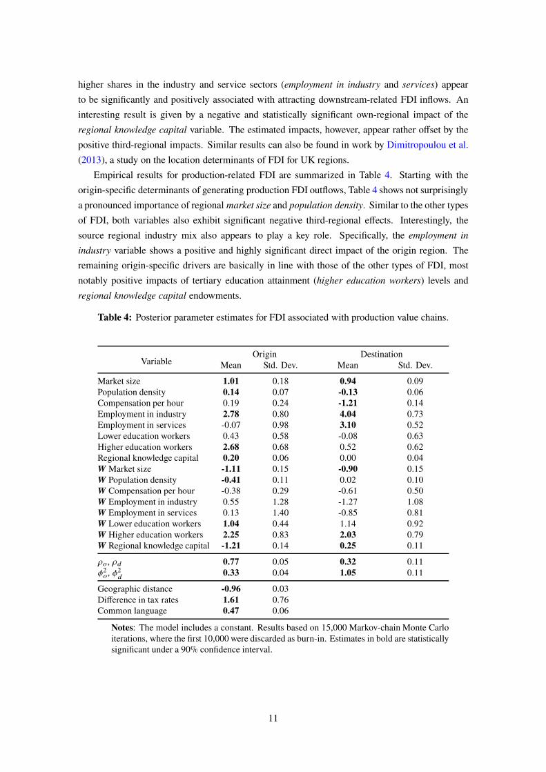
Empirical results for production-related FDI are summarized in Table 4. Starting with the
origin-specific determinants of generating production FDI outflows, Table 4 shows not surprisingly
a pronounced importance of regional market size and population density. Similar to the other types
of FDI, both variables also exhibit significant negative third-regional effects. Interestingly, the
source regional industry mix also appears to play a key role. Specifically, the employment in
industry variable shows a positive and highly significant direct impact of the origin region. The
remaining origin-specific drivers are basically in line with those of the other types of FDI, most
notably positive impacts of tertiary education attainment (higher education workers) levels and
regional knowledge capital endowments.
Table 4: Posterior parameter estimates for FDI associated with production value chains.
VariableOrigin Destination
Mean Std. Dev. Mean Std. Dev.
Market size 1.01 0.18 0.94 0.09Population density 0.14 0.07 -0.13 0.06Compensation per hour 0.19 0.24 -1.21 0.14Employment in industry 2.78 0.80 4.04 0.73Employment in services -0.07 0.98 3.10 0.52Lower education workers 0.43 0.58 -0.08 0.63Higher education workers 2.68 0.68 0.52 0.62Regional knowledge capital 0.20 0.06 0.00 0.04] Market size -1.11 0.15 -0.90 0.15] Population density -0.41 0.11 0.02 0.10] Compensation per hour -0.38 0.29 -0.61 0.50] Employment in industry 0.55 1.28 -1.27 1.08] Employment in services 0.13 1.40 -0.85 0.81] Lower education workers 1.04 0.44 1.14 0.92] Higher education workers 2.25 0.83 2.03 0.79] Regional knowledge capital -1.21 0.14 0.25 0.11
d>, d3 0.77 0.05 0.32 0.11q2>, q
23
0.33 0.04 1.05 0.11
Geographic distance -0.96 0.03Difference in tax rates 1.61 0.76Common language 0.47 0.06
Notes: The model includes a constant. Results based on 15,000 Markov-chain Monte Carloiterations, where the first 10,000 were discarded as burn-in. Estimates in bold are statisticallysignificant under a 90% confidence interval.
11
Inspection of the destination-specific determinants of production-related FDI, however, reveals
markedly different patterns as compared to upstream and downstream FDI. Albeit the market size
shows a similar importance, along with negative third-regional effects, the direct impact of the
population density variable shows a negative and significant sign. Our estimation results thus show
that production-oriented FDI activities are predominantly attracted by smaller regions in proximity
to urban agglomerations. For upstream and downstream activities, however, urban agglomerations
seem to play a more central role. Moreover, our results imply that regional human capital en-
dowments are particularly important for explaining upstream and downstream-oriented investment
decisions. For production activities, the importance of regional human capital endowments ap-
pears slightly less pronounced. These results corroborate the findings of Strauss-Kahn and Vives
(2009), and Defever (2006) by highlighting that industry-related location decisions typically fo-
cus on sectoral, rather than on functional aspects. The significant and positive own-regional,
destination-specific industry mix (employment in industry and services) further underpins these
findings.
For attracting production-related FDI, Table 4 shows a particularly pronounced negative impact
of the compensation per hour variable of the host region. The negative direct impact on inflows is
the strongest with a posterior mean of −1.21 for production-related activities. However, it is worth
noting that the associated third-regional impacts on inflows are insignificant for production, whereas
both downstream and upstream related FDI flows exhibit significant negative third-regional impacts.
Our findings are moreover in line with Fallon and Cook (2014) and Crescenzi et al. (2013), who
both find that locational drivers for production-related FDI flows differ from those associated with
business service activities.
Spatial-dependence and distance metrics
This subsection discusses the results for the spatial autoregressive origin and destination random
effects, as well as the estimates of intervening opportunities from the distance matrix J. In-
spection of posterior estimates for the spatial latent random effects provides significant evidence
for pronounced spatial dependence patterns in the random effects across all stages of the value
chain. This finding holds true for both source- and host-regional heterogeneity in the sample. A
comparison of their corresponding posterior means and standard deviations shows that all spatial
autoregressive parameters are estimated with a high precision. The intensity of spatial dependence
in the upstream- and downstream-specific latent unobservable effects appear similarly pronounced,
with values ranging from 0.42 to 0.58. For production-related investment activities, the difference
between d> and d3 appears more pronounced, with the former being particularly sizeable (0.77),
while the latter appears more muted.
Rather similar results for upstream, downstream and production are also reported for the
distance factors collected in matrix J. As expected, the posterior mean estimates for geographical
distance are negative and significantly differ from zero for all types of investment activities.
Moreover, the posterior standard deviations are comparatively small, indicating that the impact
of geographic distance is estimated with a high precision. Higher geographic separation of two
12
regions is thus associated with lower FDI activities, as increased distance often raises transportation,
monitoring and thus investment costs. The negative impacts reported in Tables 2, 3, and 4
are in line with recent empirical results in FDI (Leibrecht and Riedl 2014) and trade literature
(Krisztin and Fischer 2015).
Our dummy variable measuring whether a pair of regions shares an official common language
proxies the cultural distance between regions in the sample. As expected, the reported posterior
means show a positive sign and are significantly different from zero. The third distance variable
in the matrix J measures the (country-specific) difference in corporate tax rates between source
and target regions. In line with theoretical and empirical literature on the location choice of
multinationals, the tables report significant and positive impacts to regional FDI flows when
corporate tax rates in the target region are lower than in the source region (see Bellak and Leibrecht
2009 and Strauss-Kahn and Vives 2009). The estimated posterior means for the difference in tax
rates suggest that a 1% decrease in the tax rate difference between source and destination regions
results in a 1.3% and 3.5% increase in the number of FDI flows for downstream and upstream
related activities, respectively.
5 Conclusions
This paper presents an empirical study on the spatial determinants of bilateral FDI flows among
European regions. Due to data scarcity on the subnational level, previous papers typically adopt
a national perspective when analysing FDI dyads (see, for example, Leibrecht and Riedl 2014).
This paper thus provides a first spatial econometric analysis on the European regional level by
explicitly accounting for origin-, destination-, and third region-specific factors in the analysis. The
subnational perspective of our analysis allows us to study the spatial spillover mechanisms of
regional FDI flows in more detail. Unlike recent studies on the locational determinants of FDI
inflows (see, for example, Ascani et al. 2016b, or Crescenzi et al. 2013), we model FDI decision
determinants not only across destination regions but also across the origin regional dimension.
Moreover, due to the well-known need to control for spatial dependence when modelling regional
data (LeSage and Pace, 2009), we also capture spatial dependence through spatially structured
random effects associated with origin and destination regions.
Our data comes from the fDi Markets database, which contains detailed information on regional
FDI activities using media sources and company data. The data from the fDi Markets database also
contains detailed sectoral information on the functional form of the FDI activity, which allows us
to explicitly focus on FDI flows across different stages of the value chain. Specifically, the paper
studies the origin- and destination-specific determinants of upstream, downstream, and production
activities.
Our empirical results clearly indicate that both source and destination spatial dependence
plays a key role for all investment activities under scrutiny. In line with recent literature, we
find that regional market size, corporate tax rates, as well as third region effects appear to be of
particular importance for all stages in the value chain. We moreover find that production-oriented
FDI activities are predominantly attracted by smaller regions in proximity to urban agglomerations.
13

For upstream and downstream activities, however, being in the same region as urban agglomerations
seem to play a key role. Moreover, our results imply that regional human capital endowments are
particularly important for explaining upstream and downstream-oriented investment decisions. For
production activities, the importance of regional human capital endowments are less accentuated.
These results corroborate the findings of Strauss-Kahn and Vives (2009), or Defever (2006) by
highlighting that industry-related location decisions typically focus on sectoral, rather than on
functional aspects. From an origin-specific perspective of FDI activities, our empirical results
moreover clearly show that regional knowledge capital endowments appear crucial for host regions
to produce FDI outflows. Similar to the results on the destination-specific factors for FDI inflows,
we also find high education and agglomeration forces as particularly important aspects for host
regional FDI outflows.
Declarations
Funding: The research carried out in this paper was supported by funds of the Oesterreichische
Nationalbank (project number: 18116), and of the Austrian Science Fund (FWF): ZK35.
Conflict of interest: The authors declare that they have no conflict of interest.
Ethical approval: This article does not contain any studies with human participants or animals
performed by any of the authors.
References
Ascani A, Crescenzi R and Iammarino S (2016a) Economic institutions and the location strategies
of European multinationals in their geographic neighborhood. Economic Geography 92(4),
401–429
Ascani A, Crescenzi R and Iammarino S (2016b) What drives European multinationals to the
European Union neighbouring countries? A mixed-methods analysis of Italian investment
strategies. Environment and Planning C: Government and Policy 34(4), 656–675
Baltagi BH, Egger P and Pfaffermayr M (2007) Estimating models of complex FDI: Are there
third-country effects? Journal of Econometrics 140(1), 260–281
Basile R and Kayam S (2015) Empirical literature on location choice of multinationals. In
Complexity and Geographical Economics. Springer, 325–351
Bellak C and Leibrecht M (2009) Do low corporate income tax rates attract FDI? – Evidence from
Central- and East European countries. Applied Economics 41(21), 2691–2703
Blonigen BA (2005) A review of the empirical literature on FDI determinants. Atlantic Economic
Journal 33(4), 383–403
Blonigen BA, Davies RB, Waddell GR and Naughton HT (2007) FDI in space: Spatial autoregres-
sive relationships in foreign direct investment. European Economic Review 51(5), 1303–1325
Blonigen BA and Piger J (2014) Determinants of foreign direct investment. Canadian Journal of
Economics 47(3), 775–812
14

Casi L and Resmini L (2010) Evidence on the determinants of foreign direct investment: The case
of EU regions. Eastern Journal of European Studies 1(2), 93–118
Chou KH, Chen CH and Mai CC (2011) The impact of third-country effects and economic
integration on China’s outward FDI. Economic Modelling 28(5), 2154–2163
Coughlin CC, Terza JV and Arromdee V (1991) State characteristics and the location of foreign
direct investment within the United States. The Review of Economics and Statistics 73(4),
675–683
Crescenzi R, Pietrobelli C and Rabellotti R (2013) Innovation drivers, value chains and the ge-
ography of multinational corporations in Europe. Journal of Economic Geography 14(6),
1053–1086
Crespo Cuaresma J, Doppelhofer G, Huber F and Piribauer P (2018) Human capital accumulation
and long-term income growth projections for European regions. Journal of Regional Science
58(1), 81–99
Defever F (2006) Functional fragmentation and the location of multinational firms in the enlarged
Europe. Regional Science and Urban Economics 36(5), 658–677
Dimitropoulou D, McCann P and Burke SP (2013) The determinants of the location of foreign
direct investment in UK regions. Applied Economics 45(27), 3853–3862
Dunning JH (2001) The eclectic (OLI) paradigm of international production: past, present and
future. International Journal of the Economics of Business 8(2), 173–190
Duranton G and Puga D (2005) From sectoral to functional urban specialisation. Journal of Urban
Economics 57(2), 343–370
Fallon G and Cook M (2014) Explaining manufacturing and non-manufacturing inbound FDI
location in five UK regions. Tijdschrift voor Economische en Sociale Geografie 105(3), 331–
348
Fischer MM and LeSage JP (2015) A Bayesian space-time approach to identifying and interpreting
regional convergence clubs in Europe. Papers in Regional Science 94(4), 677–702
Frühwirth-Schnatter S, Frühwirth R, Held L and Rue H (2009) Improved auxiliary mixture sampling
for hierarchical models of non-Gaussian data. Statistics and Computing 19(4), 479–492
Frühwirth-Schnatter S, Halla M, Posekany A, Pruckner G and Schober T (2013) Applying standard
and semiparametric Bayesian IV on health economic data. In Bayesian Young Statisticians
Meeting (BAYSM). 1–4
Frühwirth-Schnatter S and Wagner H (2006) Auxiliary mixture sampling for parameter-driven
models of time series of counts with applications to state space modelling. Biometrika 93(4),
827–841
Garretsen H and Peeters J (2009) FDI and the relevance of spatial linkages: Do third-country
effects matter for Dutch FDI? Review of World Economics 145(2), 319–338
Geweke J (1991) Evaluating the accuracy of sampling-based approaches to the calculation of
posterior moments, volume 196. Federal Reserve Bank of Minneapolis, Research Department
Minneapolis, MN, USA
Henderson JV and Ono Y (2008) Where do manufacturing firms locate their headquarters? Journal
of Urban Economics 63(2), 431–450
15

Huber F, Fischer MM and Piribauer P (2017) The role of US based FDI flows for global output
dynamics. Macroeconomic Dynamics 23(3), 943–973
Koch W and LeSage JP (2015) Latent multilateral trade resistance indices: Theory and evidence.
Scottish Journal of Political Economy 62(3), 264–290
Krisztin T and Fischer MM (2015) The gravity model for international trade: Specification and
estimation issues. Spatial Economic Analysis 10(4), 451–470
Leibrecht M and Riedl A (2014) Modeling FDI based on a spatially augmented gravity model:
Evidence for Central and Eastern European Countries. The Journal of International Trade &
Economic Development 23(8), 1206–1237
LeSage JP and Fischer MM (2012) Estimates of the impact of static and dynamic knowledge
spillovers on regional factor productivity. International Regional Science Review 35(1), 103–
127
LeSage JP, Fischer MM and Scherngell T (2007) Knowledge spillovers across Europe: Evidence
from a Poisson spatial interaction model with spatial effects. Papers in Regional Science 86(3),
393–421
LeSage JP and Pace RK (2009) Introduction to Spatial Econometrics. CRC Press, Boca Raton
London New York
Markusen JR (1995) The boundaries of multinational enterprises and the theory of international
trade. Journal of Economic Perspectives 9(2), 169–189
Pace RK and Barry RP (1997) Quick computation of regressions with a spatially autoregressive
dependent variable. Geographical Analysis 29(3), 291–297
Pintar N, Sargant B and Fischer MM (2016) Austrian outbound foreign direct investment in Europe:
A spatial econometric study. Romanian Journal of Regional Science 10(1), 1–22
Poelhekke S and van der Ploeg F (2009) Foreign direct investment and urban concentrations:
Unbundling spatial lags. Journal of Regional Science 49(4), 749–775
Raftery AE and Lewis S (1992) How many iterations in the Gibbs sampler? In Bernardo JM,
Berger J, Dawid AP and Smith AFM, eds., Bayesian Statistics 4. Oxford University Press,
Oxford, 763–773
Regelink M and Elhorst JP (2015) The spatial econometrics of FDI and third country effects.
Letters in Spatial and Resource Sciences 8(1), 1–13
Ritter C and Tanner MA (1992) Facilitating the Gibbs sampler: The Gibbs stopper and the griddy-
Gibbs sampler. Journal of the American Statistical Association 87(419), 861–868
Strauss-Kahn V and Vives X (2009) Why and where do headquarters move? Regional Science
and Urban Economics 39(2), 168–186
Sturgeon TJ (2008) Mapping integrative trade: Conceptualising and measuring global value chains.
International Journal of Technological Learning, Innovation and Development 1(3), 237–257
16

Appendix
Table A1: Classification of fDi Markets business functions
Classification Business activities % of classification
Upstream
Business Services 64.0Design, Development and Testing 10.8Education and Training 2.5Headquarters 12.1Information and Communication Technology and Internet Infrastructure 4.3Research and Development 6.3
Downstream
Customer Contact Centre 4.2Logistics, Distribution and Transportation 26.9Maintenance and Servicing 3.4Sales, Marketing and Support 62.1Shared Services Centre 2.0Technical Support Centre 1.4
Production
Construction 21.0Electricity 5.3Extraction 0.3Manufacturing 72.1Recycling 1.3
Notes: The last column indicates the percent of industry activities per FDI classification. The values are based on thetotal observed FDI flows in the fDi Markets database targeting the selected NUTS-2 regions in the period 2003-2011.
17

Table A2: List of regions in the study.
Austria France [continued] Hungary Poland [continued] UK
Burgenland (AT) Languedoc-Roussillon Dél-Alföld Lódzkie Bedfordshire and Hertfordshire
Kärnten Limousin Dél-Dunántúl Lubelskie Berkshire, Buckinghamshire and
Niederösterreich Lorraine Észak-Alföld Lubuskie Oxfordshire
Oberösterreich Midi-Pyrénées Észak-Magyarország Malopolskie Cheshire
Salzburg Nord - Pas-de-Calais Közép-Dunántúl Mazowieckie Cornwall and Isles of Scilly
Steiermark Pays de la Loire Közép-Magyarország Opolskie Cumbria
Tirol Picardie Nyugat-Dunántúl Podkarpackie Derbyshire and Nottinghamshire
Vorarlberg Poitou-Charentes Ireland Podlaskie Devon
Wien Provence-Alpes-Côte d’Azur Border, Midland and Western Pomorskie Dorset and Somerset
Belgium Rhône-Alpes Southern and Eastern Slaskie East Anglia
Prov. Antwerpen Germany Italy Swietokrzyskie East Wales
Prov. Brabant Wallon Arnsberg Abruzzo Warminsko-Mazurskie East Yorkshire and
Prov. Hainaut Berlin Basilicata Wielkopolskie Northern Lincolnshire
Prov. Liège Brandenburg Calabria Zachodniopomorskie Eastern Scotland
Prov. Limburg (BE) Braunschweig Campania Portugal Essex
Prov. Luxembourg (BE) Bremen Emilia-Romagna Alentejo Gloucestershire, Wiltshire and
Prov. Namur Chemnitz Friuli-Venezia Giulia Algarve Bristol
Prov. Oost-Vlaanderen Darmstadt Lazio Área Metropolitana de Lisboa Greater Manchester
Prov. Vlaams-Brabant Detmold Liguria Centro (PT) Hampshire and Isle of Wight
Prov. West-Vlaanderen Dresden Lombardia Norte Herefordshire, Worcestershire
Région de Bruxelles-Capitale Düsseldorf Marche Romania and Warwickshire
Bulgaria Freiburg Molise Bucuresti - Ilfov Highlands and Islands
Severen tsentralen Gießen Piemonte Centru Inner London
Severoiztochen Hamburg Provincia Autonoma di Bolzano/ Nord-Est Kent
Severozapaden Hannover Bozen Nord-Vest Lancashire
Yugoiztochen Karlsruhe Provincia Autonoma di Trento Sud - Muntenia Leicestershire, Rutland and
Yugozapaden Kassel Puglia Sud-Est Northamptonshire
Yuzhen tsentralen Koblenz Sardegna Sud-Vest Oltenia Lincolnshire
Czech Republic Köln Sicilia Vest Merseyside
Jihovýchod Leipzig Toscana Slovakia North Eastern Scotland
Jihozápad Lüneburg Umbria Bratislavský kraj North Yorkshire
Moravskoslezsko Mecklenburg-Vorpommern Valle d’Aosta/Vallée d’Aoste Stredné Slovensko Northern Ireland (UK)
Praha Mittelfranken Veneto Východné Slovensko Northumberland and Tyne and
Severovýchod Münster Latvia Západné Slovensko Wear
Severozápad Niederbayern Latvija Slovenia Outer London
Strední Cechy Oberbayern Lithuania Vzhodna Slovenija Shropshire and Staffordshire
Strední Morava Oberfranken Lietuva Zahodna Slovenija South Western Scotland
Denmark Oberpfalz Luxemburg Sweden South Yorkshire
Hovedstaden Rheinhessen-Pfalz Luxemburg Mellersta Norrland Surrey, East and West Sussex
Midtjylland Saarland Netherlands Norra Mellansverige Tees Valley and Durham
Nordjylland Sachsen-Anhalt Drenthe Östra Mellansverige West Midlands
Sjælland Schleswig-Holstein Flevoland Övre Norrland West Wales and The Valleys
Syddanmark Schwaben Friesland (NL) Småland med öarna West Yorkshire
Estonia Stuttgart Gelderland Stockholm
Eesti Thüringen Groningen Sydsverige
Finland Trier Limburg (NL) Västsverige
Åland Tübingen Noord-Brabant Spain
Etelä-Suomi Unterfranken Noord-Holland Andalucía
Helsinki-Uusimaa Weser-Ems Overijssel Aragón
Länsi-Suomi Greece Utrecht Cantabria
Pohjois-ja Itä-Suomi Anatoliki Makedonia, Thraki Zeeland Castilla y León
France Attiki Zuid-Holland Castilla-la Mancha
Alsace Dytiki Ellada Norway Cataluña
Aquitaine Dytiki Makedonia Agder og Rogaland Comunidad de Madrid
Auvergne Ionia Nisia Hedmark og Oppland Comunidad Foral de Navarra
Basse-Normandie Ipeiros Nord-Norge Comunidad Valenciana
Bourgogne Kentriki Makedonia Oslo og Akershus Extremadura
Bretagne Kriti Sør-Østlandet Galicia
Centre (FR) Notio Aigaio Trøndelag Illes Balears
Champagne-Ardenne Peloponnisos Vestlandet La Rioja
Corsica Sterea Ellada Poland País Vasco
Franche-Comté Thessalia Dolnoslaskie Principado de Asturias
Haute-Normandie Voreio Aigaio Kujawsko-Pomorskie Región de Murcia
Île de France
18
A.1 Detailed description of the Bayesian Markov-chain Monte Carlo algorithm
This section provides a detailed description of the employed Bayesian Markov-chain Monte
Carlo (MCMC) algorithm. A similar version is employed by LeSage et al. (2007), who use
such a modelling strategy for estimation of knowledge spillovers (measured in terms of patent-
ing dyads) in European regions. Specifically, their estimation approach relies on work by
Frühwirth-Schnatter and Wagner (2006), who introduce a Bayesian auxiliary mixture sampling
approach for non-Gaussian distributed data. This approach builds on a hierarchical data augmen-
tation procedure by introducing H8 + 1 latent variables for each observation H8, where H8 denotes
the 8-th element of y (with 8 = 1, ..., #).
In order to alleviate the implied computational burden, we rely on an improved version of this
auxiliary mixture sampling algorithm (Frühwirth-Schnatter et al., 2013). The algorithm tremen-
dously reduces the number of latent parameters per observation. Specifically, the required number
of latent parameters is reduced from H8 + 1 to at most two per observation for Poisson distributed
data (Frühwirth-Schnatter et al., 2013).
From a statistical point of view, _8 from Eq. (2.1) can be interpreted as a parameter in a Poisson
process describing occurring events in a given time interval, where _8 denotes the 8-th element
of the Poisson mean ,. For illustration, imagine sorting all unique values of the observed FDI
flows from lowest to highest. The Poisson process can be viewed as modeling – given a specific
number of FDI flows – the probability of jumping from one unique value to the next. These
two quantities can be characterized as so-called arrival and inter-arrival times. Motivated by this
formulation, the distribution itself can be described using merely arrival and inter-arrival times,
derived from the rate of the process _8. The expected value of arrival time of H8 is 1/_8 and it
follows a Gamma distribution with shape one and rate equal to H8. The inter-arrival times are by
definition independent and arise from an exponential distribution with rate equal to _8. Based on
this definition, we can model _8 if we sample from the inter-arrival time g81 between H8 and H8 + 1,
as well as for H8 > 0, the arrival g82 time for H8. The main contribution of Frühwirth-Schnatter et al.
(2009) is that they introduce auxiliary variables for g81 and g82, conditional on H8.
For this purpose let us define the latent variables g81 and g82, based on the properties of arrival
and inter-arrival times:
g81 =
b81
_8, b81 ∼ E(1) (A.1)
g82 =
b82
_8, b81 ∼ G(H8, 1) ∀ H8 > 0, (A.2)
where E(·) denotes the exponential and G(·, ·) the Gamma distribution. The arrival times g82 only
apply for H8 > 0, since zero values have by definition no arrival time. Eqs. (A.1) and (A.2) can be
log-linearized in the following fashion:
− ln g81 = ln_8 + Y81, Y81 = − ln b81 (A.3)
− ln g82 = ln_8 + Y82, Y82 = − ln b82 ∀ H8 > 0, (A.4)
19
where for H8 = 0 only Eq. (A.3) is defined. Evidently, if Y81 and Y82 would be Gaussian this would
imply a linear model, which could be easily sampled from. While Y81 and Y82 are not Gaussian
per se, the distributions can be approximated by a mixture of Gaussians, from which sampling can
easily be achieved (Frühwirth-Schnatter et al., 2009).
In order to obtain a model which is conditionally Gaussian, the non-normal density can be
approximated by a mixture of & (a) normal components, where a denotes the shape parameter of
a Gamma distribution. For sampling Y81 we can set a = 1, and in the case of sampling Y81 the rate
a would be equal to H8. Therefore, the mixture of normal components can be generalised for both
distributions. Thus, the mixture distribution is given by:
?Y (Y |a) ∼
& (a)∑
@=1
F@ (a)N[
Y |<@ (a), B@ (a)]
, (A.5)
where F@ (a) denotes the weight, <@ (a) the mean, and B@ (a) the variance. These components, as
well as & (a) directly depend on the choice of a. Values for all these parameters conditional on a
are provided in Frühwirth-Schnatter et al. (2009). To approximate the Poisson process through the
Gaussian mixture in Eq. (A.5), the additional latent discrete variable a81, and additionally in cases
of H8 > 0 the discrete variable a82 are introduced.
Given g81 and a81 and additionally for the case of H8 > 0 g82 and a82, the conditional posterior
of the Poisson model’s slope parameters are Gaussian:
− ln g81 = ln _8 + < (1) + Y81, Y81 |a81 ∼ N [0, B(1)] (A.6)
− ln g82 = ln _8 + < (a82) + Y82, Y82 |a82 ∼ N [0, B(a82)] ∀ H8 > 0. (A.7)
We can easily sample from the distributions given in Eqs. (A.6) and (A.7) and therefore construct
an efficient Gibbs sampling algorithm (for a detailed description, see Section A.1 in the Appendix).
For Bayesian estimation, we have to define prior distributions for all parameters in the model.
We follow the canonical approach and use a Gaussian prior setup for the parameters U0, #>, #3,
$� , %>, and %3 with zero mean and a relatively large prior variance of 104. We follow LeSage et al.
(2007) in our choice of priors for the spatially structured random effect vectors and set a normal
prior structure )> and )3, with with zero mean and q2G (GGGG)
−1 variance, where G ∈ [>, 3] and
GG = O= − dG]. For the variance of the random effects q2G we employ an inverse Gamma prior
with rate equal to 5 and the shape parameter to 0.05. Following LeSage et al. (2007), we elicit a
non-informative uniform prior specification dG ∼ U(−1, 1).
A.2 The Gibbs sampling scheme
Let us collect the explanatory variables from Eq. (2.1) in an # × % (with % = 1 + 4?- +
?�) matrix ` = [*# , ^>, ^3 , J,]>^>,]3^3] and $ = [U0, #′>, #
′3, $
′�, %′>, %
′3]
′. Thus, , =
exp (`$ +\>)> +\3)3).
Moreover, let us denote the number of non-zero observations in y as #H>0. Then, let #+ =
# + #H>0 and let the #+ × 1 vector y+ be y+ = [y ′, y′H>0]
′, where yH>0 contains all elements of y
20

which are greater than zero. Moreover, let the #+ × % matrix `+ be `+ = [` ′, `′H>0]
′, where the
matrix `H>0 contains all rows of ` corresponding to H: > 0. In a similar fashion, we augment the
dummy observation matrices \> and \3 and denote the resulting #+ × = matrices as \+> and \+
3.
Accordingly we order the auxiliary variables corresponding to Y81 and Y82 and collect them
into the following #+ × 1 auxiliary variable vectors as 3 = [g11, ..., g# 1, g12, ..., g#H>02] and
. = [a11, ..., a# 1, a12, ..., a#H>02]. Based on this, we define the #+ × #+ variance matrix .
Additionally – based on the definition of the Gaussian mixtures in Eqs. (A.6 - A.7) – an #+ × 1
vector of working responses y can be obtained conditional on 3 and ., so that y = < (.) − ln 3.
Given appropriate starting values the following Gibbs sampling algorithm can be devised:
I. Sample $ from its conditional Gaussian distribution ?($ |·) ∼ N (�$-$,�$), where
�$ =
(
`′+
−1`+ + �−1$
)−1-$ = `′
+−1( y −\+
>)> −\+3)3) + �
−1$ -
$.
�$ denotes the % × % prior variance matrix and -$
the % × 1 matrix of prior means.
II. Sample ) G from their conditional distributions ?() G |·) ∼ N (�)G -)G ,�)G ), where
�)G =
(
q−2G GG
′GG +\+′
G −1\+
G
)−1-)G = \+′
G −1 ( y − `+$ −\+
G) G)
.
III. We sample q2G from the conditional posterior, which is inverse Gamma distributed and given
as ?(q2G |·) ∼ IG(BG , 1/EG) where:
BG = (= + BG)/2 EG =
(
) ′GG
′GGG) G + BGEG
)
/2.
BG
and EG
denote the prior rate and shape parameters of the inverse gamma distribution
IG(·, ·).
IV. For dG the conditional posterior distribution is:
?(dG |·) ∝ |GG | exp
(
−1
2q2G
) ′GG
′GGG) G
)
.
Unfortunately, this is not a well-known distribution, thus – as is standard in the spatial
econometric literature – we resort to a griddy Gibbs step (Ritter and Tanner 1992) in order
to sample from the conditional posterior for dG .6 For this purpose candidate values d∗Gare sampled from d∗G = N(dG, cdG ), where cdG is the proposal density variance, which is
adaptively adjusted using the procedure from LeSage and Pace (2009) and thus is constrained
to a desired interval by the means of rejection sampling. The candidate values are evaluated
using their full posterior distributions7.
6An alternative, however, computationally more intensive approach also frequently used in the spatial econometricliterature involves a Metropolis-Hastings step for the spatial autoregressive parameter (see, for example, LeSage and Pace2009).
7In practice it is costly to evaluate the log-determinant directly. Instead we use an adapted version of the log-determinant approximation by Pace and Barry (1997) for pre-calculation.
21

V. For 8 = 1, ..., # we sample g81 from b81 ∼ Ex(,8) and set g81 = 1 + b81. If H: > 0 then
we additionally sample g82 from B(H8, 1) (where B(·) denotes the Beta distribution) and set
g81 = 1 − g82 + b81.
VI. For 8 = 1, ..., # we sample a81 from the discrete distribution involving the mixture of normal
distributions with A = 1, ..., & (1):
?(a81 = A |·) ∝ FA (1)N [− ln g81 − ln _8 |<A (1), BA (1)]
and for H8 > 1 we additionally sample a82 from the discrete distribution (with A = 1, ..., & (H8)):
?(a82 = A |·) ∝ FA (H8)N [− ln g82 − ln _8 |<A (H8), BA (H8)] .
With the sampled values for 3 and ., we update y = ln 3 − < (.) and .
This concludes the Gibbs sampling algorithm. The Markov-chain Monte Carlo algorithm cycles
through steps I. to VI. � times and excludes the initial �0 draws as burn-ins. Inference regarding
the parameters is subsequently conducted using the remaining � − �0 draws.8
8Whether the MCMC algorithm converged can be easily verified using convergence diagnostics by Geweke (1991)or Raftery and Lewis (1992). For the present application we utilised an implementation of these convergence diagnosticsfrom the R coda package.
22


![GreyOne: Data Flow Sensitive Fuzzingforming implicit data flows. It causes either under-taint if the implicit flows are ignored, or over-taint if such flows are all counted [19]](https://img.pdfslide.us/doc/110x75/6112bfcf77132112af284db7/greyone-data-flow-sensitive-fuzzing-forming-implicit-data-iows-it-causes-either.jpg)