MODELING ELECTROSPINNING PROCESS

AND

A NUMERICAL SCHEME USING LATTICE BOLTZMANN METHOD TO

SIMULATE VISCOELASTIC FLUID FLOWS

A Thesis

by

SATISH KARRA

Submitted to the Office of Graduate Studies ofTexas A&M University

in partial fulfillment of the requirements for the degree of

MASTER OF SCIENCE

May 2007

Major Subject: Mechanical Engineering

MODELING ELECTROSPINNING PROCESS

AND

A NUMERICAL SCHEME USING LATTICE BOLTZMANN METHOD TO

SIMULATE VISCOELASTIC FLUID FLOWS

A Thesis

by

SATISH KARRA

Submitted to the Office of Graduate Studies ofTexas A&M University

in partial fulfillment of the requirements for the degree of

MASTER OF SCIENCE

Approved by:

Co-Chairs of Committee, Arun R. SrinivasaSharath Girimaji

Committee Member, N.K. AnandHead of Department, Dennis O’Neal

May 2007

Major Subject: Mechanical Engineering

iii

ABSTRACT

Modeling Electrospinning Process

and

A Numerical Scheme using Lattice Boltzmann Method to Simulate Viscoelastic

Fluid Flows. (May 2007)

Satish Karra, B.Tech, Indian Institute of Technology Madras, Chennai, India

Co–Chairs of Advisory Committee: Dr. Arun R. SrinivasaDr. Sharath Girimaji

In the recent years, researchers have discovered a multitude of applications

using nanofibers in fields like composites, biotechnology, environmental engineer-

ing, defense, optics and electronics. This increase in nanofiber applications needs

a higher rate of nanofiber production. Electrospinning has proven to be the best

nanofiber manufacturing process because of simplicity and material compatibility.

Study of effects of various electrospinning parameters is important to improve the

rate of nanofiber processing. In addition, several applications demand well-oriented

nanofibers. Researchers have experimentally tried to control the nanofibers using

secondary external electric field. In the first study, the electrospinning process is

modeled and the bending instability of a viscoelastic jet is simulated. For this, the

existing discrete bead model is modified and the results are compared, qualitatively,

with previous works in literature. In this study, an attempt is also made to simulate

the effect of secondary electric field on electrospinning process and whipping instabil-

ity. It is observed that the external secondary field unwinds the jet spirals, reduces

the whipping instability and increases the tension in the fiber.

iv

Lattice Boltzmann method (LBM) has gained popularity in the past decade as

the method is easy implement and can also be parallelized. In the second part of this

thesis, a hybrid numerical scheme which couples lattice Boltzmann method with finite

difference method for a Oldroyd-B viscoelastic solution is proposed. In this scheme,

the polymer viscoelastic stress tensor is included in the equilibrium distribution func-

tion and the distribution function is updated using SRT-LBE model. Then, the local

velocities from the distribution function are evaluated. These local velocities are used

to evaluate local velocity gradients using a central difference method in space. Next,

a forward difference scheme in time is used on the Maxwell Upper Convected model

and the viscoelastic stress tensor is updated. Finally, using the proposed numerical

method start-up Couette flow problem for Re = 0.5 and We = 1.1, is simulated. The

velocity and stress results from these simulations agree very well with the analytical

solutions.

v

ACKNOWLEDGMENTS

I would like to thank Dr. Arun Srinivasa for his support and motivation through-

out this work and for his guidance on vital decisions related to my career. I would

also like to sincerely thank Dr. Girimaji for giving me an opportunity to work with

him and helping me financially.

I would also like to thank my parents who have been there for me through good

and bad times. Finally, I would like to thank my friends and colleagues: Vijay

Idimadakala, Hari, Swaroop, Chaitanya, Anshul, Vijay Sathyamurthi, Nandagopalan

and Praveen.

vi

TABLE OF CONTENTS

CHAPTER Page

I INTRODUCTION . . . . . . . . . . . . . . . . . . . . . . . . . . 1

II MODELING ELECTROSPINNING PROCESS . . . . . . . . . 4

A. Introduction . . . . . . . . . . . . . . . . . . . . . . . . . . 4

B. Nanofiber processing . . . . . . . . . . . . . . . . . . . . . 5

C. Applications of nanofibers . . . . . . . . . . . . . . . . . . 7

D. Electrospinning . . . . . . . . . . . . . . . . . . . . . . . . 9

E. Instabilities in jet formation observed in electrospinning . . 11

F. Importance of electrospinning . . . . . . . . . . . . . . . . 14

G. Modeling and simulation of electrospinning . . . . . . . . . 15

H. Objectives of this study . . . . . . . . . . . . . . . . . . . 17

I. Discrete bead model: method and governing equations . . 18

J. Results and discussion . . . . . . . . . . . . . . . . . . . . 24

K. Conclusions . . . . . . . . . . . . . . . . . . . . . . . . . . 31

III A NUMERICAL SCHEME USING LATTICE BOLTZMANN

METHOD TO SIMULATE VISCOELASTIC FLUID FLOWS . 34

A. Introduction . . . . . . . . . . . . . . . . . . . . . . . . . . 34

B. Lattice Boltzmann method . . . . . . . . . . . . . . . . . . 36

C. Continuum equations for viscoelastic fluids . . . . . . . . . 39

D. Numerical scheme . . . . . . . . . . . . . . . . . . . . . . . 40

E. Validation of the method . . . . . . . . . . . . . . . . . . . 42

F. Conclusions and future work . . . . . . . . . . . . . . . . . 45

IV SUMMARY . . . . . . . . . . . . . . . . . . . . . . . . . . . . . 48

REFERENCES . . . . . . . . . . . . . . . . . . . . . . . . . . . . . . . . . . . 49

APPENDIX A . . . . . . . . . . . . . . . . . . . . . . . . . . . . . . . . . . . 58

VITA . . . . . . . . . . . . . . . . . . . . . . . . . . . . . . . . . . . . . . . . 60

vii

LIST OF FIGURES

FIGURE Page

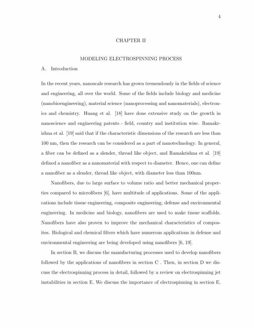
1 Schematic of drawing process [19]. Each fiber is drawn from a

micro-droplet of polymer solution using a micropipette. . . . . . . . . 5

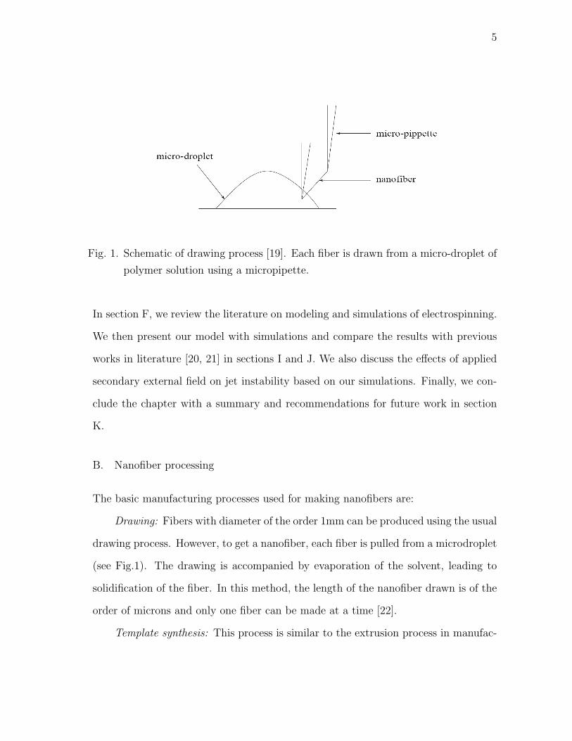
2 Schematic of template synthesis [23]. Pressure is applied on the

polymer and the polymer extrudes through a nanoporous template. . 6

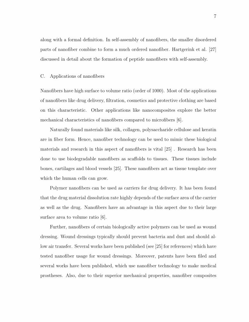
3 Schematic showing the application of nanofibers in the fields of

biotechnology and biomedical, environmental engineering, defense

and other applications like optics [6, 19]. . . . . . . . . . . . . . . . . 8

4 Schematic of basic electrospinning set-up with the whipping in-

stability of jet. Typically a potential difference of 15 – 20 KV is

applied across the syringe with polymer solution and the copper

collector. Here, H is the distance between the syringe and collec-

tor (which is typically of the order of 15 – 20 cm). The secondary

instabilities [20] are not shown. . . . . . . . . . . . . . . . . . . . . . 10

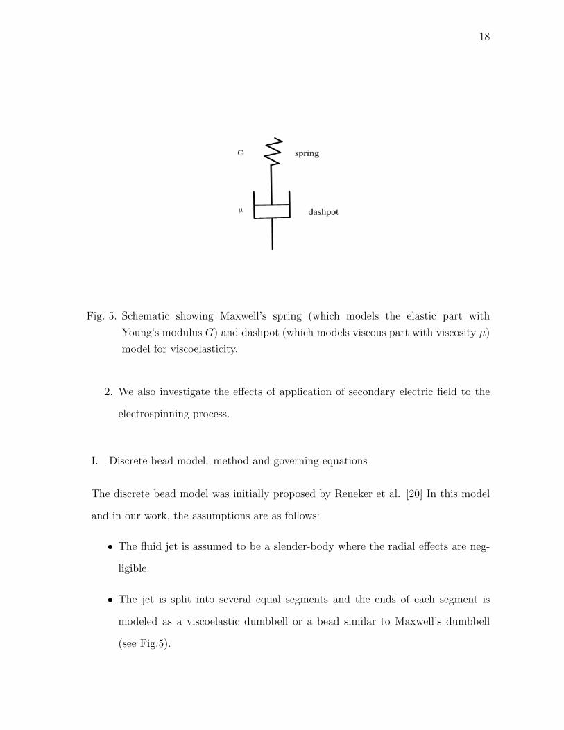
5 Schematic showing Maxwell’s spring (which models the elastic

part with Young’s modulus G) and dashpot (which models viscous

part with viscosity µ) model for viscoelasticity. . . . . . . . . . . . . 18

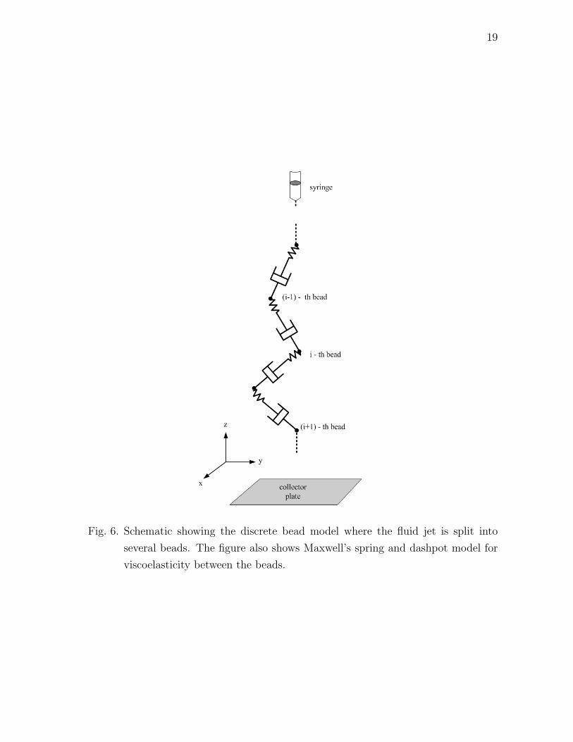
6 Schematic showing the discrete bead model where the fluid jet is

split into several beads. The figure also shows Maxwell’s spring

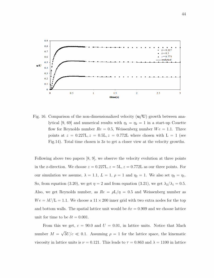
and dashpot model for viscoelasticity between the beads. . . . . . . . 19

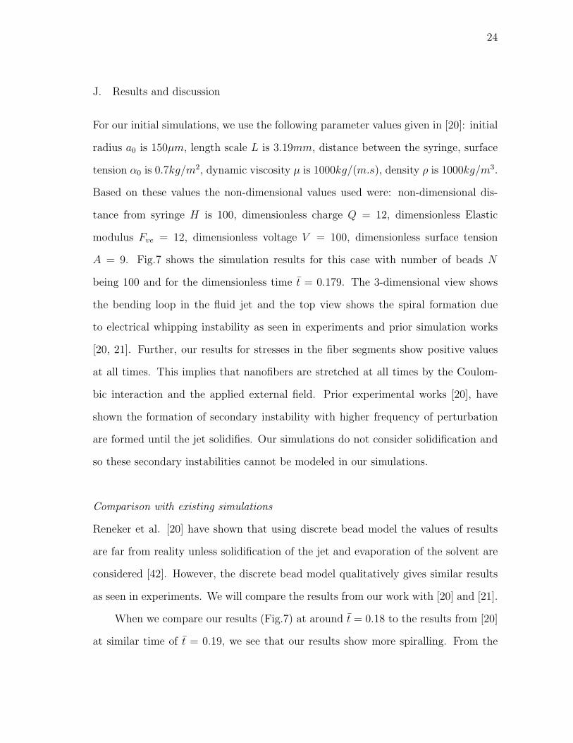
7 Typical result for the discrete particle model showing the bending

loop in the jet. Top view shows that the envelope of the jet

trajectory is a cone. The number of beads for this simulation

N = 100 and non-dimensionalized time t̄ = 0.183. . . . . . . . . . . . 23

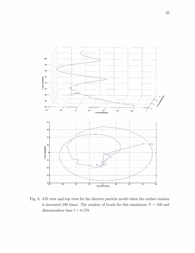
8 3-D view and top view for the discrete particle model when the

surface tension is increased 100 times. The number of beads for

this simulation N = 100 and dimensionless time t̄ = 0.179. . . . . . . 25

viii

FIGURE Page

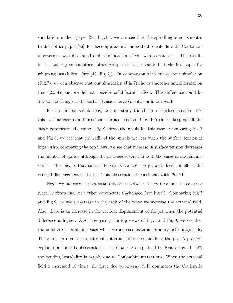
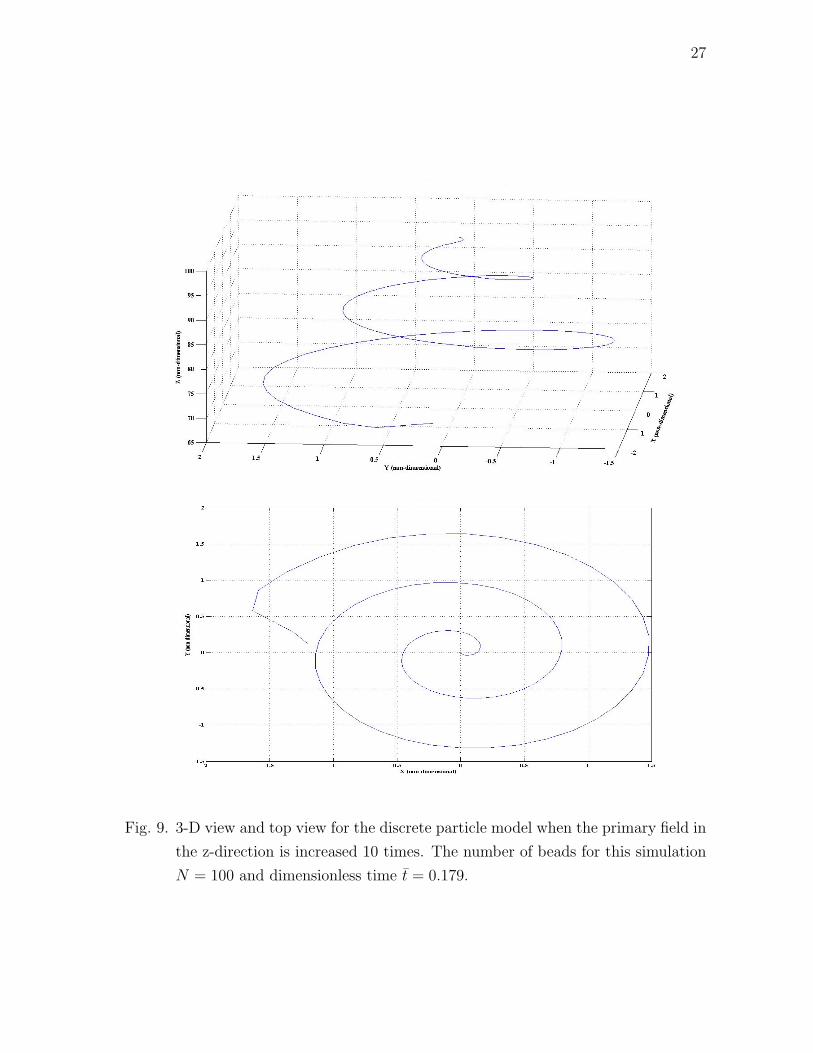
9 3-D view and top view for the discrete particle model when the

primary field in the z-direction is increased 10 times. The number

of beads for this simulation N = 100 and dimensionless time t̄ = 0.179. 27

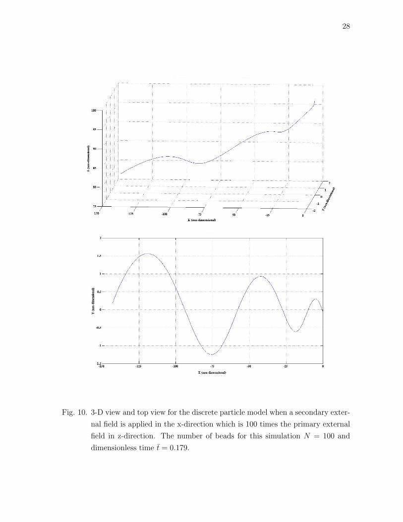
10 3-D view and top view for the discrete particle model when a

secondary external field is applied in the x-direction which is 100

times the primary external field in z-direction. The number of

beads for this simulation N = 100 and dimensionless time t̄ = 0.179. 28

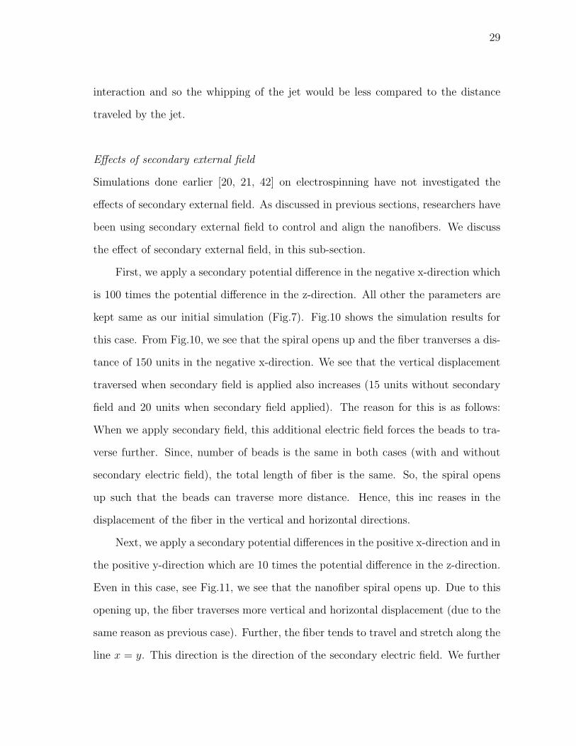
11 3-D view and top view for the discrete particle model when a

secondary external fields are applied in the x-direction and y-

direction which are 10 times the primary external field in z-direction.

The number of beads for this simulation N = 100 and dimension-

less time t̄ = 0.179. . . . . . . . . . . . . . . . . . . . . . . . . . . . . 30

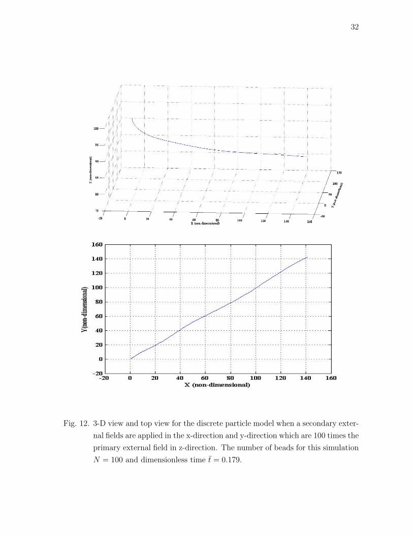
12 3-D view and top view for the discrete particle model when a

secondary external fields are applied in the x-direction and y-

direction which are 100 times the primary external field in z-

direction. The number of beads for this simulation N = 100

and dimensionless time t̄ = 0.179. . . . . . . . . . . . . . . . . . . . . 32

13 D3Q19 lattice . . . . . . . . . . . . . . . . . . . . . . . . . . . . . . . 37

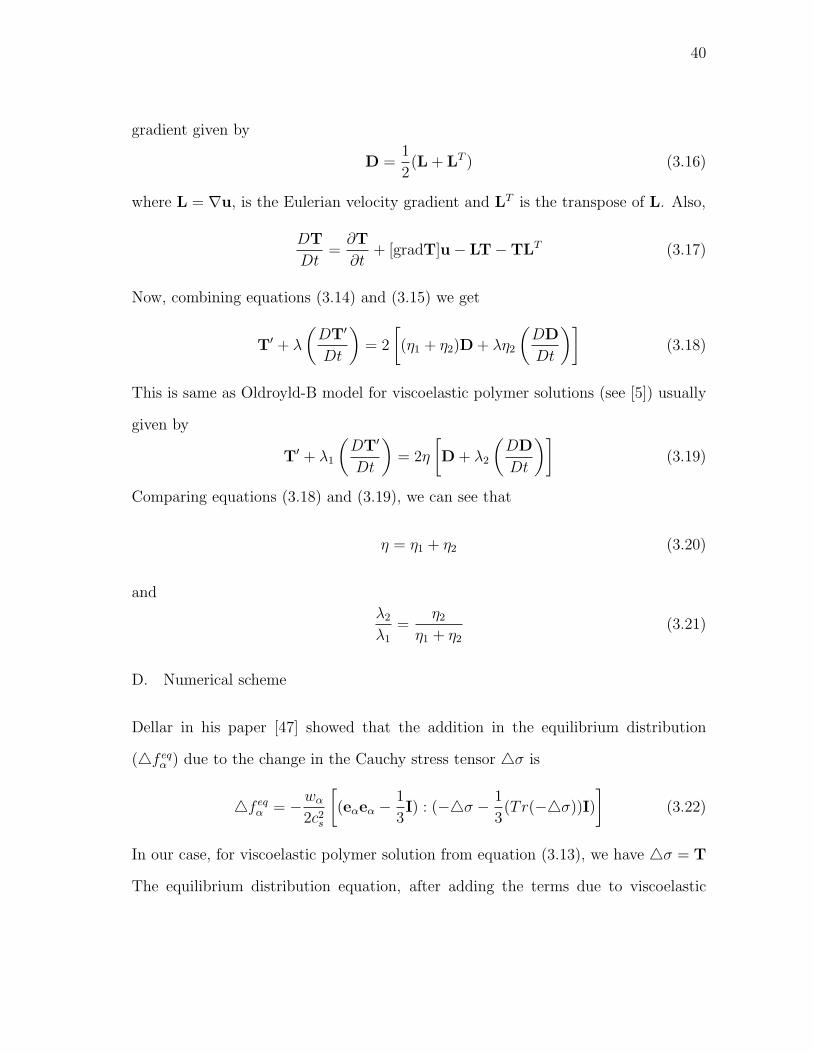
14 Schematic showing start-up Couette flow. The lower plate is at

rest at all times while the upper plate moves with a constant

velocity ‘U’, H(t) is the heaviside function. . . . . . . . . . . . . . . . 41

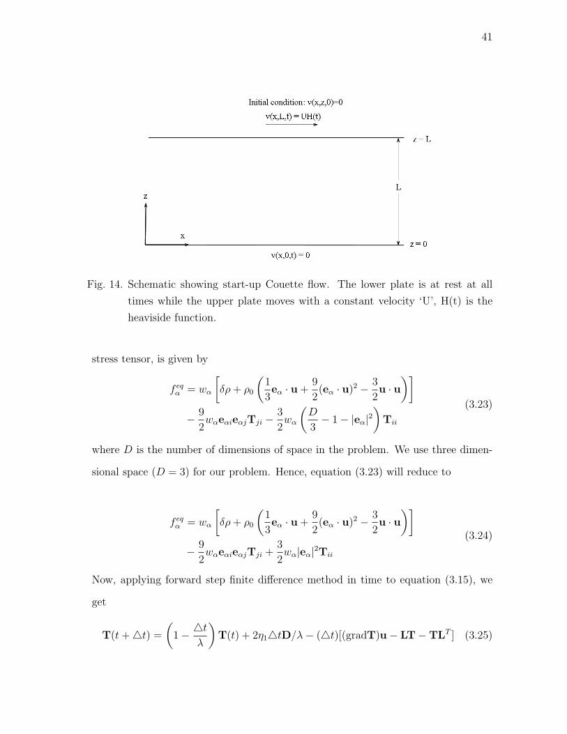
15 Comparison of the non-dimensionalized velocity (u/U) growth

between analytical [9, 69] and numerical results with η1 = η2 = 1

in a start-up Couette flow for Reynolds number Re = 0.5, Weis-

senberg number We = 1.1. Three points at z = 0.227L, z =

0.5L, z = 0.772L where chosen with L = 1 (see Fig.14) and the

total time is 8s. . . . . . . . . . . . . . . . . . . . . . . . . . . . . . 43

16 Comparison of the non-dimensionalized velocity (u/U) growth

between analytical [9, 69] and numerical results with η1 = η2 = 1

in a start-up Couette flow for Reynolds number Re = 0.5, Weis-

senberg number We = 1.1. Three points at z = 0.227L, z =

0.5L, z = 0.772L where chosen with L = 1 (see Fig.14). Total

time chosen is 3s to get a closer view at the velocity growths. . . . . 44

ix

FIGURE Page

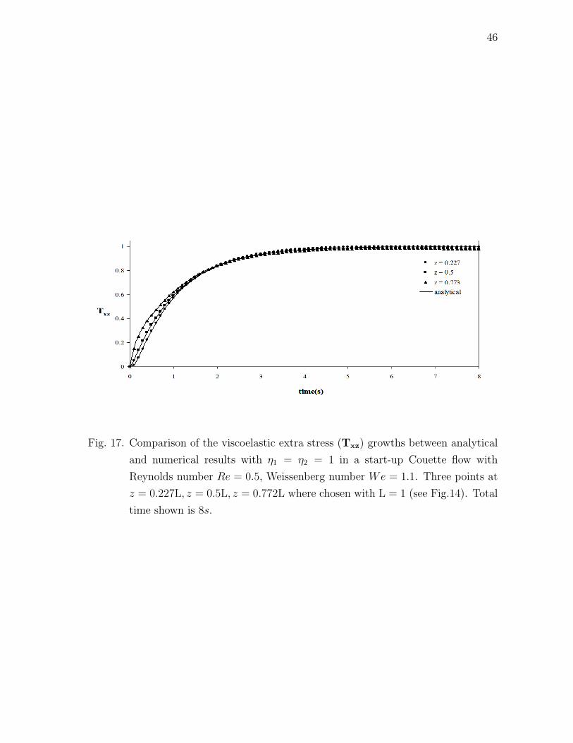
17 Comparison of the viscoelastic extra stress (Txz) growths between

analytical and numerical results with η1 = η2 = 1 in a start-

up Couette flow with Reynolds number Re = 0.5, Weissenberg

number We = 1.1. Three points at z = 0.227L, z = 0.5L, z =

0.772L where chosen with L = 1 (see Fig.14). Total time shown is 8s. 46

1

CHAPTER I

INTRODUCTION

Substances like polymers, emulsions, colloids which show both solid-like and fluid-

like behavior are viscoelastic in nature. However, when an external stress is applied,

a viscoelastic fluid’s transient response is much larger than the time scales of the

instrument used [1]. In a viscoelastic fluid, the stress tensor depends on the history

of the deformation gradient [2]. Due to their vast applications, viscoelastic fluids have

been studied for several decades to understand the phenomena associated with it. For

instance, polymers are widely used in applications like automobiles, textile industry

and composites. In these applications, the polymer is usually used in a fluid form,

either as a melt or either dissolved in a solvent. These polymers are shaped commonly

by spinning process or through extrusion process. The problem of spinning has been

studied for several decades and some of theoretical works in this area have been

done by Kannan and Rajagopal [3] and Bechtel [4]. In the extrusion of viscoelastic

fluids several interesting and complex phenomena, some of them due to instability,

have been observed. These phenomena include extrude die swell, sharkskin effect,

spurting. Several theoretical and experimental, have been done to explain and model

these phenomena [5, 1].

Another viscoelastic flow problem which has been studied in the recent years is

the electrospinning jet formation problem. Polymer nanofiber research has gained

momentum in the last decade due to the vast applications of nanofibers [6]. Electro-

spinning, which was initially developed by Formhals (See [6] for reference) in 1934, was

re-discovered a decade ago, as a powerful process to produce nanofibers. Electrospin-

The journal model is IEEE Transactions on Automatic Control.

2

ning has been found to have several advantages over classical spinning processes and

other nanofiber manufacturing processes. Unlike, classical spinning process which

mainly uses gravity and externally applied tension, electrospinning uses externally

applied electric field, as driving force. In electrospinning, instabilities like Taylor

instability and whipping instability were also observed; though the reason behind

these instabilities is still not clear. Further, in electrospinning nanofibers form a

random mesh and certain nanofiber applications demand highly oriented nanofibers.

Research is being done to control the nanofiber orientation using a secondary external

field [7]. Modeling and simulation of electrospinning process will help us understand

the following:

• the cause for whipping instability.

• the dependence of jet formation and jet instability on the process parameters

and fluid properties, for better jet control and higher production rate.

• the effect of secondary external field on jet instability and fiber orientation.

With this motivation, we attempt to model and simulate the jet formation in elec-

trospinning, in the first part of this thesis.

Also, several works have been done to solve and understand viscoelastic flow prob-

lems like die-swelling extrusion problem and jet buckling problem using traditional

numerical techniques like finite volume [8], finite difference [9] and finite element [10].

These techniques, in general, have been found to be less effective and more computa-

tionally intensive compared to a more recently developed lattice Boltzmann method

[11, 12]. LBM involves simple arithmetic and so this method easy to implement. Fur-

ther, LBM can be can parallelized as the computations are local. Hence, LBM can

be used for large-scale computations [13] and problems involving complex fluids [13],

3

colloidal suspensions [14] and moving boundaries [15] can been easily solved using

LBM. Due to these advantages of LBM over traditional CFD schemes, a LBM based

technique which models viscoelastic fluid behavior is valuable. However, very few

works have been done in this aspect [16, 17]. Hence, in the second part of this thesis,

we explore the use of LBM to viscoelastic fluid flows.

The objectives of the thesis can be summarized as follows:

• Model and simulate electrospinning jet flow and whipping instability.

• Develop a hybrid numerical using the lattice Boltzmann method to solve the

viscoelastic flow problems.

The outline of the thesis is as follows: In chapter II, we first discuss the back-

ground of electrospinning and review the previous works on elecstrospinning modeling

and simulation. Then, we discuss our model and simulations for the electrospinning

process along with the basic assumptions. In chapter III, we first review previous

works that used lattice Boltzmann method. We also present the continuum gov-

erning equations for viscoelastic fluid flows. We then develop our hybrid numerical

scheme using LBM and finite difference method for Oldroyd-B polymer solutions. We

then simulate start-up Couette flow with our scheme and compare the results with

the analytical solution. Finally, we summarize the thesis in chapter IV.

4

CHAPTER II

MODELING ELECTROSPINNING PROCESS

A. Introduction

In the recent years, nanoscale research has grown tremendously in the fields of science

and engineering, all over the world. Some of the fields include biology and medicine

(nanobioengineering), material science (nanoprocessing and nanomaterials), electron-

ics and chemistry. Huang et al. [18] have done extensive study on the growth in

nanoscience and engineering patents - field, country and institution wise. Ramakr-

ishna et al. [19] said that if the characteristic dimensions of the research are less than

100 nm, then the research can be considered as a part of nanotechnology. In general,

a fiber can be defined as a slender, thread like object, and Ramakrishna et al. [19]

defined a nanofiber as a nanomaterial with respect to diameter. Hence, one can define

a nanofiber as a slender, thread like object, with diameter less than 100nm.

Nanofibers, due to large surface to volume ratio and better mechanical proper-

ties compared to microfibers [6], have multitude of applications. Some of the appli-

cations include tissue engineering, composite engineering, defense and environmental

engineering. In medicine and biology, nanofibers are used to make tissue scaffolds.

Nanofibers have also proven to improve the mechanical characteristics of compos-

ites. Biological and chemical filters which have numerous applications in defense and

environmental engineering are being developed using nanofibers [6, 19].

In section B, we discuss the manufacturing processes used to develop nanofibers

followed by the applications of nanofibers in section C . Then, in section D we dis-

cuss the electrospinning process in detail, followed by a review on electrospinning jet

instabilities in section E. We discuss the importance of electrospinning in section E.

5

Fig. 1. Schematic of drawing process [19]. Each fiber is drawn from a micro-droplet of

polymer solution using a micropipette.

In section F, we review the literature on modeling and simulations of electrospinning.

We then present our model with simulations and compare the results with previous

works in literature [20, 21] in sections I and J. We also discuss the effects of applied

secondary external field on jet instability based on our simulations. Finally, we con-

clude the chapter with a summary and recommendations for future work in section

K.

B. Nanofiber processing

The basic manufacturing processes used for making nanofibers are:

Drawing: Fibers with diameter of the order 1mm can be produced using the usual

drawing process. However, to get a nanofiber, each fiber is pulled from a microdroplet

(see Fig.1). The drawing is accompanied by evaporation of the solvent, leading to

solidification of the fiber. In this method, the length of the nanofiber drawn is of the

order of microns and only one fiber can be made at a time [22].

Template synthesis: This process is similar to the extrusion process in manufac-

6

Fig. 2. Schematic of template synthesis [23]. Pressure is applied on the polymer and

the polymer extrudes through a nanoporous template.

turing. Nanoporous filtration membrane is used as a template (see Fig.2). Nanofibers

are produced when the polymer is extruded through these nanopores under pressure.

Martin [23] has produced nanotubules of various metals, carbons and semiconductor

materials using this process.

Gelation: Initially, a gel is made using pre-determined amounts of polymer and

solvent followed by phase separation and gel formation. Finally, nanofiber matrix

forms when the gel is frozen and freeze-dried [24, 25]. Notice that in this method a

matrix forms in this process instead of a single fiber.

Self-assembly: In nano-manufacturing, a material of desired dimensions can be

processed either using top-down or bottom-up technique [19, 25]. In the top-down

method, a larger size of the material is cut till the desired size is achieved. On

the other hand, in the bottom-up method, the desired size is achieved by building

from molecules. Self-assembly is a bottom-up technique and in self-assembly, stable

and ordered structures are formed from disordered entities of molecules. Typically,

non-covalent bonds like hydrogen bonds and electrostatic forces are responsible for

self-assembly [25]. See [26] for detailed description of self-assembly and applications

7

along with a formal definition. In self-assembly of nanofibers, the smaller disordered

parts of nanofiber combine to form a much ordered nanofiber. Hartgerink et al. [27]

discussed in detail about the formation of peptide nanofibers with self-assembly.

C. Applications of nanofibers

Nanofibers have high surface to volume ratio (order of 1000). Most of the applications

of nanofibers like drug delivery, filtration, cosmetics and protective clothing are based

on this characteristic. Other applications like nanocomposites explore the better

mechanical characteristics of nanofibers compared to microfibers [6].

Naturally found materials like silk, collagen, polysaccharide cellulose and keratin

are in fiber form. Hence, nanofiber technology can be used to mimic these biological

materials and research in this aspect of nanofibers is vital [25] . Research has been

done to use biodegradable nanofibers as scaffolds to tissues. These tissues include

bones, cartilages and blood vessels [25]. These nanofibers act as tissue template over

which the human cells can grow.

Polymer nanofibers can be used as carriers for drug delivery. It has been found

that the drug material dissolution rate highly depends of the surface area of the carrier

as well as the drug. Nanofibers have an advantage in this aspect due to their large

surface area to volume ratio [6].

Further, nanofibers of certain biologically active polymers can be used as wound

dressing. Wound dressings typically should prevent bacteria and dust and should al-

low air transfer. Several works have been published (see [25] for references) which have

tested nanofiber usage for wound dressings. Moreover, patents have been filed and

several works have been published, which use nanofiber technology to make medical

prostheses. Also, due to their superior mechanical properties, nanofiber composites

8

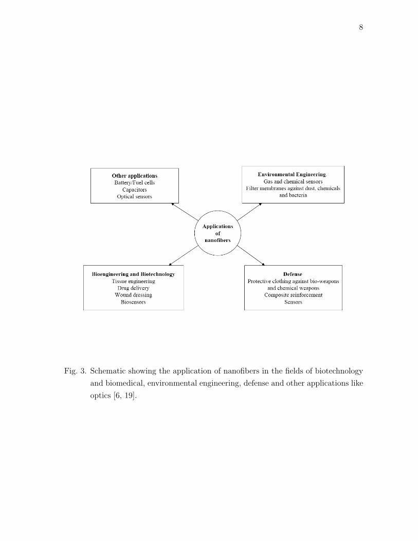
Fig. 3. Schematic showing the application of nanofibers in the fields of biotechnology

and biomedical, environmental engineering, defense and other applications like

optics [6, 19].

9

are used in fillers for dental purposes.

Due to high surface area to volume ratio, nanofibers can be used for molecular

separation and filtration. Further, nanofiber meshes can be used as skin care masks

as they block dust particles. In addition, the higher surface area allows quicker

transfer rate of the mask additives. Nanofiber meshes can act as protective clothing

from biological as well as chemical agents because of their excellent potential for

filtration. Finally, nanofibers can be used to make bio-sensors, and to preserve and

store biologically active substances like enzymes (see Zhang et al. [25] for references

with regard to biotechnology and biomedical applications).

As the electric conductivity highly depends on the surface area, nanofibrous

membranes made from a conductive material can be used as electrode for batter-

ies [6]. Nanofibrous membranes can also be used as highly responsive fluorescence

optical sensors [28]. Also, nanofibers from electrospinning can be used to make tem-

plates in template synthesis to develop nanotubes that cannot be processed using

electrospinning [29]. Fig.3 shows an overview of various applications of nanofibers.

D. Electrospinning

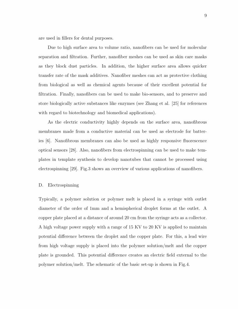
Typically, a polymer solution or polymer melt is placed in a syringe with outlet

diameter of the order of 1mm and a hemispherical droplet forms at the outlet. A

copper plate placed at a distance of around 20 cm from the syringe acts as a collector.

A high voltage power supply with a range of 15 KV to 20 KV is applied to maintain

potential difference between the droplet and the copper plate. For this, a lead wire

from high voltage supply is placed into the polymer solution/melt and the copper

plate is grounded. This potential difference creates an electric field external to the

polymer solution/melt. The schematic of the basic set-up is shown in Fig.4.

10

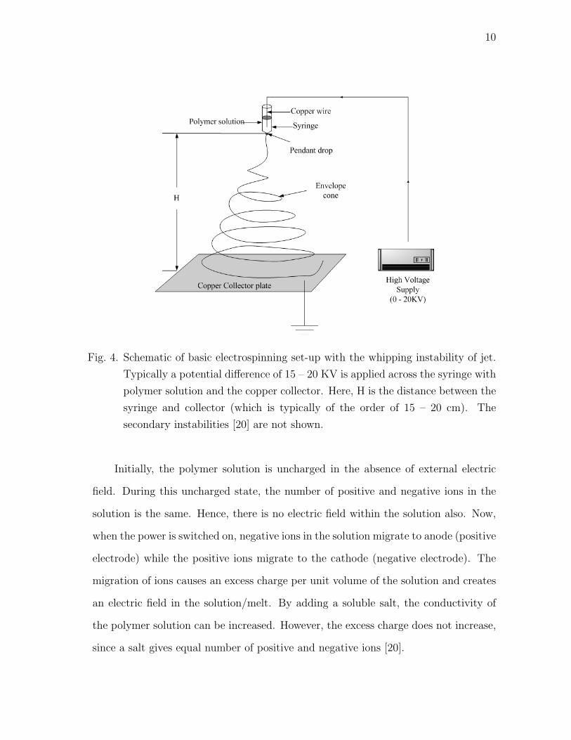
Fig. 4. Schematic of basic electrospinning set-up with the whipping instability of jet.

Typically a potential difference of 15 – 20 KV is applied across the syringe with

polymer solution and the copper collector. Here, H is the distance between the

syringe and collector (which is typically of the order of 15 – 20 cm). The

secondary instabilities [20] are not shown.

Initially, the polymer solution is uncharged in the absence of external electric

field. During this uncharged state, the number of positive and negative ions in the

solution is the same. Hence, there is no electric field within the solution also. Now,

when the power is switched on, negative ions in the solution migrate to anode (positive

electrode) while the positive ions migrate to the cathode (negative electrode). The

migration of ions causes an excess charge per unit volume of the solution and creates

an electric field in the solution/melt. By adding a soluble salt, the conductivity of

the polymer solution can be increased. However, the excess charge does not increase,

since a salt gives equal number of positive and negative ions [20].

11

Now, as the potential difference is increased, the hemispherical droplet elongates

to form a prolate and finally tends to a conical shape known as the Taylor cone

[30, 31]. At a particular threshold potential difference, when the forces due to the

electric field and the electrostatic repulsion overcome the surface tension forces, jet

initiates. The jet remains axisymmetric for some distance. Then an instability called

bending or whipping instability starts. This instability makes the jet to loop in spirals

with increasing radius. The envelope of this loop or curve is a cone. Further, the

electric field accelerates the jet and so the jet velocity increases. This leads to a

decrease in the jet diameter (diameter decreases to an order of 10-100 nm), by mass

conservation. In addition, the electrostatic repulsion between due to excess charges

in the solution stretches the jet. This stretching also decreases the jet diameter.

The polymer solution content in the syringe or capillary decreases in the process

and is usually supplied continuously through a syringe pump. The volumetric flow of

the polymer solution varies from 1µl/min to 1ml/min. Further, the solvent evaporates

and the jet solidifies as it reaches the collector plate. Finally, a mesh of randomly

oriented solid nanofibers forms on the collector plate.

E. Instabilities in jet formation observed in electrospinning

Initially, a pendant droplet of the polymer solution/melt forms at the end of the

syringe. When the force due to potential difference exceeds the force due to surface

tension, a jet initiates. Taylor [30] studied the jet formation from the electrically

charged pendant droplet. Taylor showed that a charged droplet destabilizes when

the force due to its own electric field exceeds the surface tension force. He also

showed, theoretically, that as the potential on the droplet surface is increased to

its critical value (i.e., at the potential which initiates instability) the shape of the

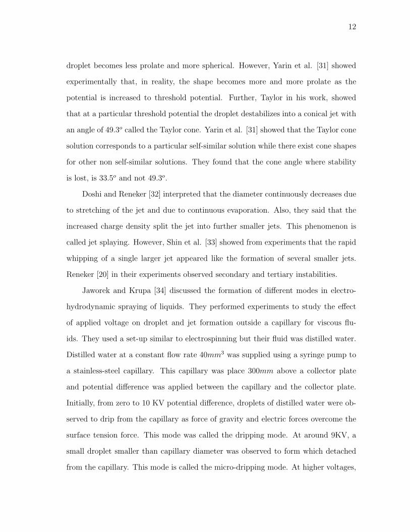
12

droplet becomes less prolate and more spherical. However, Yarin et al. [31] showed

experimentally that, in reality, the shape becomes more and more prolate as the

potential is increased to threshold potential. Further, Taylor in his work, showed

that at a particular threshold potential the droplet destabilizes into a conical jet with

an angle of 49.3o called the Taylor cone. Yarin et al. [31] showed that the Taylor cone

solution corresponds to a particular self-similar solution while there exist cone shapes

for other non self-similar solutions. They found that the cone angle where stability

is lost, is 33.5o and not 49.3o.

Doshi and Reneker [32] interpreted that the diameter continuously decreases due

to stretching of the jet and due to continuous evaporation. Also, they said that the

increased charge density split the jet into further smaller jets. This phenomenon is

called jet splaying. However, Shin et al. [33] showed from experiments that the rapid

whipping of a single larger jet appeared like the formation of several smaller jets.

Reneker [20] in their experiments observed secondary and tertiary instabilities.

Jaworek and Krupa [34] discussed the formation of different modes in electro-

hydrodynamic spraying of liquids. They performed experiments to study the effect

of applied voltage on droplet and jet formation outside a capillary for viscous flu-

ids. They used a set-up similar to electrospinning but their fluid was distilled water.

Distilled water at a constant flow rate 40mm3 was supplied using a syringe pump to

a stainless-steel capillary. This capillary was place 300mm above a collector plate

and potential difference was applied between the capillary and the collector plate.

Initially, from zero to 10 KV potential difference, droplets of distilled water were ob-

served to drip from the capillary as force of gravity and electric forces overcome the

surface tension force. This mode was called the dripping mode. At around 9KV, a

small droplet smaller than capillary diameter was observed to form which detached

from the capillary. This mode is called the micro-dripping mode. At higher voltages,

13

11-20 KV, the liquid elongated in the direction of the electric field and jets formed.

However, the high electric field detached these jets and the detached jets split into

several smaller droplets. This mode was called the spindle mode. When the potential

difference was in the range 20-25 KV, these jets oscillated. Further increase of the

voltage to around 30 KV lead to axisymmetric conical jets. In these jets two types

of instabilities were observed: varicose and kink. In varicose instability the axis of

the jet remained the same but waves were generated on the surface of the jet. While

in kink instability, the axis of the jet moved irregularly away from the axis of the

capillary. Further in the second type of instability, the jet was observed to split into

several droplets. This mode was called as conical jet mode. This final mode is also

observed in the electrospinning process.

Hohman et al. [35, 36] in their papers identified mainly two types of instability

in an electrospinning jet: Rayleigh instability and whipping instability. Note that

this Rayleigh instability in electrospinning is equivalent to the varicose instability in

the experiments performed by Jaworek and Krupa. While the whipping instability

mentioned by Hohman et al. is similar to the kink instability seen by Jaworek and

Krupa.

Hohman et al. in their first paper [35] developed a stability analysis for the ax-

isymmetric Rayleigh instability as well as the non-axisymmetric whipping instability

in Newtonian fluids. According to them, the Rayleigh instability due to electrical

forces is equivalent to the surface tension based Rayleigh instability. Further, they

observed that in the absence of the surface charges, the Rayleigh instability dominated

while increase in field and surface charge density improved the whipping instability.

In addition, it was found that the whipping conducting instability strongly depended

on the jet fluid parameters like conductivity, viscosity and dielectric constant.

14

F. Importance of electrospinning

Comparison of electrospinning with classical fiber spinning

In classical spinning (melt-spinning or dry spinning) process, the jet diameter highly

depends on the orifice diameter. Typically, the diameter of the orifice is of the order

of 0.1 mm. To reduce the diameter of the fiber, the jet is stretched due to constant

tension from the roller. The other end of the jet solidifies as it rolls. Other forces

acting on the jet are the forces due to surface tension and gravity. Now, in order to

get a final diameter of the order or nanometer, one method is to increase the distance

between the jet orifice and the roller. But to get such high draw ratio, the distance

between the orifice and the roller should be of the order of several kilometers. Such

high distances will: (a) increase the cost of production, (b) cause jet break-up due to

Rayleigh instability. The other way to get a nanometer order diameter is to increase

the tension to large values. Such high tension can lead to mechanical fracture of the

fiber jet [21]. On the other hand, in electrospinning the distance between the source

and collector is only of the order of 20cm and at such small distance we get nanofibers.

In electrospinning, the causes for jet diameter decrease are: (a) the stretching due

to the electro-static repulsion between the charges in the polymer solution, (b) the

acceleration of the jet. Hence, electrospinning is a much better process than classical

fiber spinning to make fibers with nanometer diameters.

Comparison of electrospinning with other nanofiber processing methods

In section B, we discussed the various polymer nanofiber manufacturing methods.

Drawing, as mentioned, is not a continuous process and only one fiber is drawn at a

time. Similarly, gelation and self-assembly are laboratory based processes and rate

of nanofiber production is very slow. In template synthesis, though we can get more

15

than one nanofiber at a time, the process is not continuous and nanofibers that are

only several microns in length are produced. On the other hand, electrospinning is

continuous process and nanofibers upto several meters in length can be produced with-

out breaking. Hence, electrospinning has tremendous advantage over other nanofiber

processing techniques.

Other advantages of electrospinning process are:(a) simplicity: electrospinning

is easy to set up, (b) material compatibility: about 50 polymers have shown to be

compatible with electrsopinning [19, 6]. Huang et al.[6] provide a list of: polymers

that have been used, various solvents for each polymer and the concentrations of the

polymer in the solvent. The applications of the polymer nanofibers along with their

possible uses have also been shown in the same paper. Also, a list of polymers that

have been used in melt form rather than in a solution form, is given in the paper.

Due to above mentioned advantages of electrospinning process, researchers in

the nanofiber field have identified the importance and potential of electrospinning for

nanofiber production. Currently, development of better electrospinning techniques is

a major part of nanofiber research [6, 37]. Nanofiber material characterization and

nanofiber applications are the other major areas of nanofiber research.

G. Modeling and simulation of electrospinning

Although electrospinning gives continuous fibers, with the current knowledge electro-

spinning cannot be used for mass production [6]. Theron et al. [38] used multiple

jets to improve the production rate. The other issue of current importance is con-

trolling the nanofibers. In electrospinning, the nanofibers form a random mesh on

the collector plate. However, some of the applications of nanofibers in device fabrica-

tion like microelectronics [39] and tissue engineering [7] need well-oriented nanofibers.

16

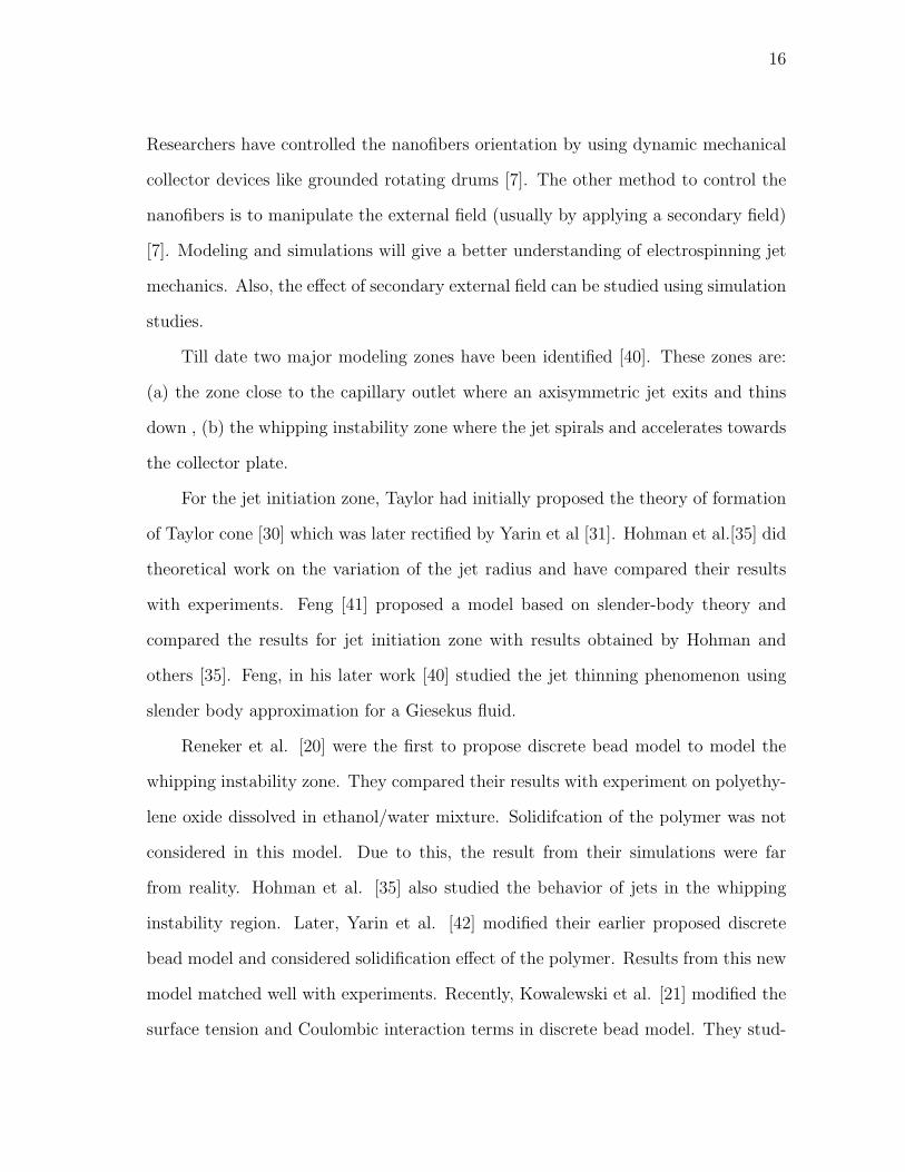
Researchers have controlled the nanofibers orientation by using dynamic mechanical

collector devices like grounded rotating drums [7]. The other method to control the

nanofibers is to manipulate the external field (usually by applying a secondary field)

[7]. Modeling and simulations will give a better understanding of electrospinning jet

mechanics. Also, the effect of secondary external field can be studied using simulation

studies.

Till date two major modeling zones have been identified [40]. These zones are:

(a) the zone close to the capillary outlet where an axisymmetric jet exits and thins

down , (b) the whipping instability zone where the jet spirals and accelerates towards

the collector plate.

For the jet initiation zone, Taylor had initially proposed the theory of formation

of Taylor cone [30] which was later rectified by Yarin et al [31]. Hohman et al.[35] did

theoretical work on the variation of the jet radius and have compared their results

with experiments. Feng [41] proposed a model based on slender-body theory and

compared the results for jet initiation zone with results obtained by Hohman and

others [35]. Feng, in his later work [40] studied the jet thinning phenomenon using

slender body approximation for a Giesekus fluid.

Reneker et al. [20] were the first to propose discrete bead model to model the

whipping instability zone. They compared their results with experiment on polyethy-

lene oxide dissolved in ethanol/water mixture. Solidifcation of the polymer was not

considered in this model. Due to this, the result from their simulations were far

from reality. Hohman et al. [35] also studied the behavior of jets in the whipping

instability region. Later, Yarin et al. [42] modified their earlier proposed discrete

bead model and considered solidification effect of the polymer. Results from this new

model matched well with experiments. Recently, Kowalewski et al. [21] modified the

surface tension and Coulombic interaction terms in discrete bead model. They stud-

17

ied the effects of various parameters like viscosity, elasticity and surface tension on

jet stability, in their Jaworeck and Krupa also performed rigorous theoretical study

and modeled the various modes of electrohydrodynamics.

Huang et al. [6] mentioned techniques using molecular dynamics modeling single

nanofiber. According to them, Monte Carlo method, which stochastically determines

properties, can be used to model single nanofibers. The other method uses deter-

ministic molecular dynamics in which the configuration of the nanofiber molecules is

determined using Newton’s laws.

H. Objectives of this study

As discussed in section G, modeling and simulation of electrospinning jet will give

us better understanding of the process. Hence, in this part of the work, we model

and simulate the electrospinning jet and the whipping instability. Also, as discussed,

control and organization of nanofibers is crucial. Although there are experimental

works in literature which analyze the effect of secondary external field [7], there are

no simulation works. In this work, we use our simulations to study the effect of field

manipulation on jet whipping instability. The specific objectives of this part of the

thesis are as follows:

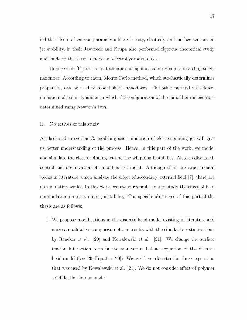
1. We propose modifications in the discrete bead model existing in literature and

make a qualitative comparison of our results with the simulations studies done

by Reneker et al. [20] and Kowalewski et al. [21]. We change the surface

tension interaction term in the momentum balance equation of the discrete

bead model (see [20, Equation 20]). We use the surface tension force expression

that was used by Kowalewski et al. [21]. We do not consider effect of polymer

solidification in our model.

18

Fig. 5. Schematic showing Maxwell’s spring (which models the elastic part with

Young’s modulus G) and dashpot (which models viscous part with viscosity µ)

model for viscoelasticity.

2. We also investigate the effects of application of secondary electric field to the

electrospinning process.

I. Discrete bead model: method and governing equations

The discrete bead model was initially proposed by Reneker et al. [20] In this model

and in our work, the assumptions are as follows:

• The fluid jet is assumed to be a slender-body where the radial effects are neg-

ligible.

• The jet is split into several equal segments and the ends of each segment is

modeled as a viscoelastic dumbbell or a bead similar to Maxwell’s dumbbell

(see Fig.5).

19

Fig. 6. Schematic showing the discrete bead model where the fluid jet is split into

several beads. The figure also shows Maxwell’s spring and dashpot model for

viscoelasticity between the beads.

20

• The dumbbells are assumed to be of the same charge, which models the ex-

cess charge a unit volume of the jet. The charge on each dumbbell leads to a

Coulombic interaction between the dumbbells in the system. Also, there is no

electrical conductivity along the jet i.e., the jet is a perfect insulator.

• The background electric field caused due to potential difference is axial and

uniform (capacitor field).

• The properties are constant.

• The effects of gravity and air drag are negligible (see [20]).

• The jet initiation zone is not considered for simulations.

• The beads are of the same mass and same charge.

• Solidification of the polymer is not considered.

Fig.6 shows the three dimensional discrete bead model for the entire jet. The figure

also shows the (i− 1)-th, i-th and the (i + 1)-th beads with a spring and a dashpot

between the beads. The spring and dashpot between the beads models the viscoelas-

ticity of the polymer fluid. This was initially proposed by Maxwell [5].

Based on above mentioned assumptions, the governing equations for the entire

system are as follows: By continuity we must have,

πa2l = πa20L (2.1)

where a0, L are the initial fiber radius and fiber segment length respectively, a, l are

the fiber radius and fiber segment length at any instant.

Using Maxwell’s law for linear viscoelasticity (Spring and dashpot model – Fig.5),

the viscoelastic interaction between the fiber segment given by i-th and (i-1)-th beads

21

can be given as

1

G

dσui

dt=

1

lui

dlui

dt− 1

µσui (2.2)

while the viscoelastic interaction between the i-th and the (i+1)-th beads in given by

1

G

dσdi

dt=

1

ldi

dldi

dt− 1

µσdi (2.3)

with lui = |ri − ri−1|, lui = |ri+1 − ri−1| where ri, ri, ri+1 are the position vectors of

(i− 1)-th, i-th, (i + 1)-th beads with respect to the syringe outlet. G is the Young’s

modulus and µ is the dynamic viscosity of the fluid.

The Coulombic interaction between the i-th bead and the rest of the beads in

the system is given by

FCoulombic =N∑

j=1,j 6=i

e2

R3ij

(ri − rj) (2.4)

where Rij is the distance between i-th and j-th bead,e is the charge on each bead, N

is the total number of beads in the system.

The force due to the external electric field is given by eV0

Hwith the direction pointing

towards the collector plate and away from the syringe.

The force due to surface tension on the i-th bead due the adjacent segments can be

written as [21]

Fsurface tension = πadiαri+1 − ri

|ri+1 − ri|− πauiα

ri − ri−1

|ri − ri−1|(2.5)

where α is the surface tension. Notice that the surface tension force term is different

from the force used in [20]. Reneker et al. evaluated the surface tension based on the

average diameter for the segment joining (i−1)-th, i-th beads and the segment joining

(i + 1)-th, i-th beads. Further, jet curvature was calculated using the (i− 1)-th, i-th

22

and (i + 1)-th bead co-ordinates.

Co-ordinate system: The xy-plane is parallel to the collector plate and z-axis points

towards the syringe away from the collector plate. The projection of the syringe on

the collector plate is the origin. Finally, using above force interactions the momentum

conservation for i-th bead is

md2ri

dt=

N∑j=1,j 6=i

e2

R3ij

(ri − rj)− eV0

Hk +

πa2uiσui

lui

(ri+1 − ri)

− πa2diσdi

ldi

(ri − ri−1) + πadiαri+1 − ri

|ri+1 − ri|− πauiα

ri − ri−1

|ri − ri−1|

(2.6)

where m is the mass of the bead, k is the unit vector in the z-direction.

In this model, i = 1 is the bottom-most bead or the bead closest to the col-

lector and i = N is the top-most bead or the bead closest to the syringe. We

non-dimensionalize equation (2.6) with the scheme used by Reneker et al [20] and

solve the set of ordinary differential equations in (2.2), (2.3) and (2.6) using MAT-

LAB. Also, we add a small initial perturbation (0.001) to the x and y positions of

the bead coming out of the syringe, in our simulations. This perturbation is given to

initialize the whipping instability due to the electrical forces. In addition, a when a

bead traverses a distance of H/2000, we add a new bead to the system. This way the

distance between a bead and its adjacent bead is always the same or in other words,

all the segments have the same length. Further, we assume that the bead coming

from syringe travels at a constant velocity in the negative z direction i.e., towards the

collector plate, for sometime (similar to [21]).

23

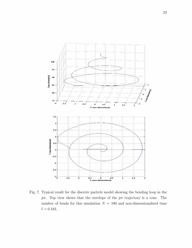
Fig. 7. Typical result for the discrete particle model showing the bending loop in the

jet. Top view shows that the envelope of the jet trajectory is a cone. The

number of beads for this simulation N = 100 and non-dimensionalized time

t̄ = 0.183.

24

J. Results and discussion

For our initial simulations, we use the following parameter values given in [20]: initial

radius a0 is 150µm, length scale L is 3.19mm, distance between the syringe, surface

tension α0 is 0.7kg/m2, dynamic viscosity µ is 1000kg/(m.s), density ρ is 1000kg/m3.

Based on these values the non-dimensional values used were: non-dimensional dis-

tance from syringe H is 100, dimensionless charge Q = 12, dimensionless Elastic

modulus Fve = 12, dimensionless voltage V = 100, dimensionless surface tension

A = 9. Fig.7 shows the simulation results for this case with number of beads N

being 100 and for the dimensionless time t̄ = 0.179. The 3-dimensional view shows

the bending loop in the fluid jet and the top view shows the spiral formation due

to electrical whipping instability as seen in experiments and prior simulation works

[20, 21]. Further, our results for stresses in the fiber segments show positive values

at all times. This implies that nanofibers are stretched at all times by the Coulom-

bic interaction and the applied external field. Prior experimental works [20], have

shown the formation of secondary instability with higher frequency of perturbation

are formed until the jet solidifies. Our simulations do not consider solidification and

so these secondary instabilities cannot be modeled in our simulations.

Comparison with existing simulations

Reneker et al. [20] have shown that using discrete bead model the values of results

are far from reality unless solidification of the jet and evaporation of the solvent are

considered [42]. However, the discrete bead model qualitatively gives similar results

as seen in experiments. We will compare the results from our work with [20] and [21].

When we compare our results (Fig.7) at around t̄ = 0.18 to the results from [20]

at similar time of t̄ = 0.19, we see that our results show more spiralling. From the

25

Fig. 8. 3-D view and top view for the discrete particle model when the surface tension

is increased 100 times. The number of beads for this simulation N = 100 and

dimensionless time t̄ = 0.179.

26

simulation in their paper [20, Fig.15], we can see that the spiralling is not smooth.

In their other paper [42], localized approximation method to calculate the Coulombic

interactions was developed and solidification effects were considered. The results

in this paper give smoother spirals compared to the results in their first paper for

whipping instability. (see [42, Fig.2]). In comparison with our current simulation

(Fig.7), we can observe that our simulation (Fig.7) shows smoother spiral formation

than [20, 42] and we did not consider solidification effect. This difference could be

due to the change in the surface tension force calculation in our work.

Further, in our simulations, we first study the effects of surface tension. For

this, we increase non-dimensional surface tension A by 100 times, keeping all the

other parameters the same. Fig.8 shows the result for this case. Comparing Fig.7

and Fig.8, we see that the radii of the spirals are less when the surface tension is

high. Also, comparing the top views, we see that increase in surface tension decreases

the number of spirals although the distance covered in both the cases is the remains

same. This means that surface tension stabilizes the jet and does not effect the

vertical displacement of the jet. This observation is consistent with [20, 21].

Next, we increase the potential difference between the syringe and the collector

plate 10 times and keep other parameters unchanged (see Fig.9). Comparing Fig.7

and Fig.9, we see a decrease in the radii of the when we increase the external field.

Also, there is an increase in the vertical displacement of the jet when the potential

difference is higher. Also, comparing the top views of Fig.7 and Fig.9, we see that

the number of spirals decrease when we increase external primary field magnitude.

Therefore, an increase in external potential difference stabilizes the jet. A possible

explanation for this observation is as follows: As explained by Reneker et al. [20]

the bending instability is mainly due to Coulombic interactions. When the external

field is increased 10 times, the force due to external field dominates the Coulombic

27

Fig. 9. 3-D view and top view for the discrete particle model when the primary field in

the z-direction is increased 10 times. The number of beads for this simulation

N = 100 and dimensionless time t̄ = 0.179.

28

Fig. 10. 3-D view and top view for the discrete particle model when a secondary exter-

nal field is applied in the x-direction which is 100 times the primary external

field in z-direction. The number of beads for this simulation N = 100 and

dimensionless time t̄ = 0.179.

29

interaction and so the whipping of the jet would be less compared to the distance

traveled by the jet.

Effects of secondary external field

Simulations done earlier [20, 21, 42] on electrospinning have not investigated the

effects of secondary external field. As discussed in previous sections, researchers have

been using secondary external field to control and align the nanofibers. We discuss

the effect of secondary external field, in this sub-section.

First, we apply a secondary potential difference in the negative x-direction which

is 100 times the potential difference in the z-direction. All other the parameters are

kept same as our initial simulation (Fig.7). Fig.10 shows the simulation results for

this case. From Fig.10, we see that the spiral opens up and the fiber tranverses a dis-

tance of 150 units in the negative x-direction. We see that the vertical displacement

traversed when secondary field is applied also increases (15 units without secondary

field and 20 units when secondary field applied). The reason for this is as follows:

When we apply secondary field, this additional electric field forces the beads to tra-

verse further. Since, number of beads is the same in both cases (with and without

secondary electric field), the total length of fiber is the same. So, the spiral opens

up such that the beads can traverse more distance. Hence, this inc reases in the

displacement of the fiber in the vertical and horizontal directions.

Next, we apply a secondary potential differences in the positive x-direction and in

the positive y-direction which are 10 times the potential difference in the z-direction.

Even in this case, see Fig.11, we see that the nanofiber spiral opens up. Due to this

opening up, the fiber traverses more vertical and horizontal displacement (due to the

same reason as previous case). Further, the fiber tends to travel and stretch along the

line x = y. This direction is the direction of the secondary electric field. We further

30

Fig. 11. 3-D view and top view for the discrete particle model when a secondary exter-

nal fields are applied in the x-direction and y-direction which are 10 times the

primary external field in z-direction. The number of beads for this simulation

N = 100 and dimensionless time t̄ = 0.179.

31

increase in the secondary potential in the positive x-direction and in the positive y-

direction to 100 times the potential difference in the z-direction. Fig.12 shows the

results for this case. We observe that the fiber stretches further along the line x = y

and is almost parallel to x = y. However, the vertical displacement in this case is

same as the vertical displacement when there is no secondary electric field (15 units

in both cases). This is because all the opened up part of the fiber did not traverse

vertically and went along the secondary field as the secondary field applied is much

stronger.

One should also note that due to the application of the secondary field, there is

an increase in the tension in the jet. So, the secondary field should be regulated such

that the tension is not large enough to break the fiber.

K. Conclusions

In this work of thesis, we modeled a fiber as a combination of several segments with

beads at the ends. We wrote the conservation of momentum for each bead which

led to a system of ordinary differential equations. These equations were solved using

the ODE solver in MATLAB and the spiral motion of nanofibers due to bending

instability was simulated. The results were compared to prior works on electrospin-

ning whipping instability simulations. Further, we investigated the effect of surface

tension on bending instability and compared the results with prior works. Also, we

studied the effect of primary external on bending instability. Finally, we looked at

the effect of secondary external electric field on whipping instability. Some of the

major conclusions of this work are:

• Surface tension stabilizes the jet.

• External applied primary potential difference decreases the jet spiral and in-

32

Fig. 12. 3-D view and top view for the discrete particle model when a secondary exter-

nal fields are applied in the x-direction and y-direction which are 100 times the

primary external field in z-direction. The number of beads for this simulation

N = 100 and dimensionless time t̄ = 0.179.

33

creases the jet vertical displacement. Thereby, it stabilizes the jet.

• External applied secondary potential difference stabilizes the fiber by unwinding

the spiral. This also increases the tension in the fiber.

• External applied secondary potential difference causes the jet to traverse in the

direction of the resultant secondary electric field.

The last point is highly useful in controlling the motion of nanofiber. However, the

secondary field increases the tension in the fiber. So, this might lead to mechanical

failure in the fiber.

Recommendations for future work

The following are the recommendations for future work:

• One can investigate the effects of secondary field considering evaporation and

solidification so that the results can be compared with experiments quantita-

tively also.

• Close to the syringe the jet is not a slender-body and the physics of the jets

in the radial direction in unknown. All the works assume the jet to be slender

body. One can investigate the mechanics in the radial direction which might

lead to a better understanding of electrospinning jet formation.

34

CHAPTER III

A NUMERICAL SCHEME USING LATTICE BOLTZMANN METHOD TO

SIMULATE VISCOELASTIC FLUID FLOWS

A. Introduction

Lattice Boltzmann method (LBM) has been extensively developed in the recent years

as an alternate to the traditional computational techniques in CFD. LBM has proven

to be a very useful method to solve flow problems involving complex fluids and com-

plex geometries. Various problems in multi-phase flow, magnetohydrodynamics, tur-

bulence, blood rheology, suspension flow and flow over porous media have been sim-

ulated using LBM. Mixing of two fluids between two parallel plates has been studied

by Rakotomalala [43]. Denniston et al. [44] developed a numerical scheme using

LBM to simulate hydrodynamics of liquid crystals. A tensorial distribution function

was defined, in their method, to recover the macroscopic governing equations from

the LB equation. Dupuis et al. [45] modeled droplet spreading . Dellar [46, 47] de-

veloped methods to solve problems in magnetohydrodynamics using LBM. Ladd and

Verberg [14] formulated a numerical scheme based on LBM to simulate particle-fluid

suspension.

Large scale complex flow problems too have been simulated as LBM codes can

be parallelized. Harting et al. [13] wrote a review on large scale computations.

They simulated complex fluid flows in porous media and complex fluid flows under

shear in their work. LBM was found to be a faster and more effective for fluid flow

simulations when compared to traditional CFD methods like finite-difference [11, 12]

and spectral methods [48]. Yu et al. [49] also showed LBM to more effective compared

to traditional NS solvers for solving turbulence problems.

35

In addition, LBM has been applied in solid mechanics. Chopard and Marconi

developed LB formulation for solids in their papers [50, 51] and used this type of for-

mulation to simulate solid-fluid interaction. Also, LBM has been extensively used in

graphics and animation industry [52, 53] to simulate real life mechanics in animations.

In biomedical research, LBM had been used to simulate blood flow and blood

clotting. Chin et al. [54] simulated interactions between two immiscible fluids using

LBM. simulated multi-phase immiscible flow using LBM with application to blood

flow. Sun and Munn simulated red blood cells flow in blood vessel using LBM. In

their simulations, they used springs to model receptor- ligand bonds. Blood flow and

blood clotting has been simulated by Bernsdorf et al. [55].

Aharonov and Rothman [56] made ad hoc modification to LBM, to simulate non-

newtonian fluids. Ginzburg and Steiner [57] simulated free surface flow with Bingham

fluids. They have used generalized LBE to evaluate the symmetric part of velocity

gradient. Using this they have used an approach similar to Aharonov and Rothman

to evaluate the viscous stress tensor. Gabbnelli et al. [58] also used LBM with ad

hoc modifications and simulated generalized Newtonian and power law fluids. Kim et

al. [59] used similar formulation to model high rate shear flow in a viscoelastic liquid

bearing.

Till date, very few methods have been developed using LBM to solve viscoelas-

ticity. Ispolatov and Grant [60] developed a LBM which uses Maxwell’s linear model.

In their method, they have considered Maxwell’s elastic stress as an external body

force. Lallemand et al. [61] formulated a multiple relaxation technique to model

viscoelastic fluid. Qian and Deng [16] introduced an extra term in the equilibrium

distribution function which models the elastic component. These three models above

models do not consider the advection of the viscoelastic stress. Such models can only

be used for small deformations (see [5]) and hence these methods [60, 61, 16] are not

36

applicable for polymer fluids flows, where the deformations are large.

Giraud et al. [17] proposed a entirely mesoscopic based formulation with multiple

relaxation times and have recovered the Jeffrey’s equation using Chapman-Enskog

method. Giupponi et al. [62] proposed a purely kinetic approach to simulate gyroid

mesophases and have shown that their method could be used to simulate viscoelastic

flow problems. In these two works, the advection of viscoelastic stress tensor have

been considered and hence correctly model viscoelastic fluid flows. Ahlrichs et al. [63]

established a method which couples lattice Boltzmann method for the fluid with a

molecular dynamics model for polymer chain. An external forcing term which models

the solvent-polymer interaction is introduced in the LB formulation.

In this chapter, we develop macroscopic based formulation which couples LBM

with finite difference. This chapter is organized as follows: In section B, the lattice

Boltzmann method is briefly described. The continuum governing equations for vis-

coelastic polymer solution that follows Oldroyd-B constitutive model is presented in

section C. The numerical method and its validation are discussed in sections D and

E respectively. In section F, we summarize and conclude the chapter.

B. Lattice Boltzmann method

The lattice Boltzmann equation using single relaxation time approximation based on

BGK collision operator is given by

fα(x + eα, t + 1)− fα(x, t) = −1

τ(fα − f eq

α ) (3.1)

where fα is the density distribution along the direction eα, f eqα is the equilibrium

density distribution along the direction eα, τ is the relaxation time of collision. (For

theory of the Boltzmann equation, see [64, 65]. For the derivation of lattice Boltzmann

37

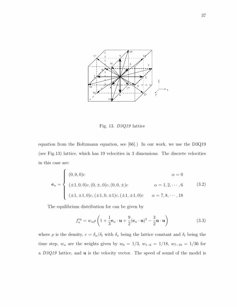
Fig. 13. D3Q19 lattice

equation from the Boltzmann equation, see [66].) In our work, we use the D3Q19

(see Fig.13) lattice, which has 19 velocities in 3 dimensions. The discrete velocities

in this case are:

eα =

(0, 0, 0)c α = 0

(±1, 0, 0)c, (0,±, 0)c, (0, 0,±)c α = 1, 2, · · · , 6

(±1,±1, 0)c, (±1, 0,±1)c, (±1,±1, 0)c α = 7, 8, · · · , 18

(3.2)

The equilibrium distribution for can be given by

f eqα = wαρ

(1 +

1

3eα · u +

9

2(eα · u)2 − 3

2u · u

)(3.3)

where ρ is the density, c = δx/δt with δx being the lattice constant and δt being the

time step, wα are the weights given by w0 = 1/3, w1−6 = 1/18, w7−18 = 1/36 for

a D3Q19 lattice, and u is the velocity vector. The speed of sound of the model is

38

cs = c/√

3 Equation (3.3) can be re-written for an incompressible flow as:

f eqα = wα

[δρ + ρ0

(1

3eα · u +

9

2(eα · u)2 − 3

2u · u

)](3.4)

where δρ is the fluctuation in the density and ρ0 is the constant mean density within

the system, which is usually set to 1. c is also usually set to 1. With the conservation

of mass and momentum given by:

δρ =∑

α

fα =∑

α

f eqα (3.5)

ρ0u =∑

α

eαfα =∑

α

eαf eqα (3.6)

The momentum flux Π can be given by the second moment of the distribution function

fα, as follows:

Π =∑

α

eαeαfα = ρuu + pI = ρuu +ρ

c2s

I (3.7)

Using multi-scale Chapman-Enskog procedure on Equation (3.1), the following

hydrodynamic equations can be derived

∂ρ

∂t+∇ρu = 0 (3.8)

∂u

∂t+ (∇u)u = −∇p +∇2u (3.9)

where p = c2sρ/ρ0 and the kinematic viscosity (ν) can be related to the relaxation

time as τ = 13(ν− 1

2). Further, while recovering the hydrodynamic equations, one can

see that the symmetric part of the velocity gradient D for the incompressible viscous

fluid can be given by [65]

Dij =1

2

(∂ui

∂xj

+∂uj

∂xi

)= − 1

2ρ0c2sτ

∑α

eαieαj[fα − f eqα ] (3.10)

39

C. Continuum equations for viscoelastic fluids

Assuming that the fluid is incompressible, the continuum/macroscopic governing

equations for the problem are given by

divu = 0 (3.11)

ρ

[∂u

∂t+ (∇u)u

]= divσ + ρb (3.12)

where ρ is the density of jet fluid, u is the velocity field vector, div is the divergence

operator, b is the body force and the Cauchy stress tensor σ is given by

σ = −pI + T′ (3.13)

In our work, we consider only a polymer solution. The stress tensor T′ corresponds to

the hydrodynamics stresses within a polymer solution which constitutes of a solvent

and polymer.

T′ = 2η2D + T (3.14)

The first part on the right side of Eq.(8) models the solvent of the solvent-polymer

solution with η2 being the solvent viscosity. The tensor T models the polymer which

is the Non-newtonian part of the solvent-polymer solution mixture which evolves as

T + λ

(DT

Dt

)= 2η1D (3.15)

Equation (3.15) is Upper Convected Maxwell model for viscoelasticity, where λ is the

relaxation time and η1 the viscosity. D is the symmertric part of the Eulerian velocity

40

gradient given by

D =1

2(L + LT ) (3.16)

where L = ∇u, is the Eulerian velocity gradient and LT is the transpose of L. Also,

DT

Dt=

∂T

∂t+ [gradT]u− LT−TLT (3.17)

Now, combining equations (3.14) and (3.15) we get

T′ + λ

(DT′

Dt

)= 2

[(η1 + η2)D + λη2

(DD

Dt

)](3.18)

This is same as Oldroyld-B model for viscoelastic polymer solutions (see [5]) usually

given by

T′ + λ1

(DT′

Dt

)= 2η

[D + λ2

(DD

Dt

)](3.19)

Comparing equations (3.18) and (3.19), we can see that

η = η1 + η2 (3.20)

and

λ2

λ1

=η2

η1 + η2

(3.21)

D. Numerical scheme

Dellar in his paper [47] showed that the addition in the equilibrium distribution

(4f eqα ) due to the change in the Cauchy stress tensor 4σ is

4f eqα = −wα

2c2s

[(eαeα −

1

3I) : (−4σ − 1

3(Tr(−4σ))I)

](3.22)

In our case, for viscoelastic polymer solution from equation (3.13), we have 4σ = T

The equilibrium distribution equation, after adding the terms due to viscoelastic

41

Fig. 14. Schematic showing start-up Couette flow. The lower plate is at rest at all

times while the upper plate moves with a constant velocity ‘U’, H(t) is the

heaviside function.

stress tensor, is given by

f eqα = wα

[δρ + ρ0

(1

3eα · u +

9

2(eα · u)2 − 3

2u · u

)]− 9

2wαeαieαjTji −

3

2wα

(D

3− 1− |eα|2

)Tii

(3.23)

where D is the number of dimensions of space in the problem. We use three dimen-

sional space (D = 3) for our problem. Hence, equation (3.23) will reduce to

f eqα = wα

[δρ + ρ0

(1

3eα · u +

9

2(eα · u)2 − 3

2u · u

)]− 9

2wαeαieαjTji +

3

2wα|eα|2Tii

(3.24)

Now, applying forward step finite difference method in time to equation (3.15), we

get

T(t +4t) =

(1− 4t

λ

)T(t) + 2η14tD/λ− (4t)[(gradT)u− LT−TLT ] (3.25)

42

where 4t is the time step.

To solve a flow problem with Oldroyd-B fluid, we propose the following algorithm for

a given domain:

First, define a scalar distribution function (f) and define the initial conditions for ρ,

u, T. For time varying from initial time to final time

1. Evaluate the equilibrium distribution function using equation (3.24).

2. Using equation (3.1), evaluate the distribution function after 1 lattice time step

and also apply the boundary conditions. Also evaluate D using equation (3.10).

3. Evaluate the macroscopic quantities u, ρ at new time step using equations (3.5)

and (3.6). Evaluate L using central difference in lattice space.

4. Update the viscoelastic extra stress tensor (T) using equation (3.25). Note that

the properties η, λ should be converted to lattice units.

5. Go to step 1.

E. Validation of the method

Tome et al. [9] validated their finite difference approach for Oldroyd-B fluid flows

using start-up Couette flow. Mompean et al. [8] also validated their finite difference

method for simulating Oldroyd-B fluid flows using start-up Couette flow. We also

simulate the start-up Couette flow for an Oldroyd-B polymer solution and compare

our results with the analytical results available in literature [9, 69].

Fig.14 shows the schematic for start-up Couette flow. The bottom plate is at

rest for all time while the upper plate is moved from rest to velocity U at time t = 0.

43

Fig. 15. Comparison of the non-dimensionalized velocity (u/U) growth between ana-

lytical [9, 69] and numerical results with η1 = η2 = 1 in a start-up Couette

flow for Reynolds number Re = 0.5, Weissenberg number We = 1.1. Three

points at z = 0.227L, z = 0.5L, z = 0.772L where chosen with L = 1 (see

Fig.14) and the total time is 8s.

44

Fig. 16. Comparison of the non-dimensionalized velocity (u/U) growth between ana-

lytical [9, 69] and numerical results with η1 = η2 = 1 in a start-up Couette

flow for Reynolds number Re = 0.5, Weissenberg number We = 1.1. Three

points at z = 0.227L, z = 0.5L, z = 0.772L where chosen with L = 1 (see

Fig.14). Total time chosen is 3s to get a closer view at the velocity growths.

Following above two papers [8, 9], we observe the velocity evolution at three points

in the z-direction. We choose z = 0.227L, z = 5L, z = 0.772L as our three points. For

our simulation we assume, λ = 1.1, L = 1, ρ = 1 and η2 = 1. We also set η2 = η1.

So, from equation (3.20), we get η = 2 and from equation (3.21), we get λ2/λ1 = 0.5.

Also, we get Reynolds number, as Re = ρL/η = 0.5 and Weissenberg number as

We = λU/L = 1.1. We choose a 11× 200 inner grid with two extra nodes for the top

and bottom walls. The spatial lattice unit would be δx = 0.909 and we choose lattice

unit for time to be δt = 0.001.

From this we get, c = 90.0 and U = 0.01, in lattice units. Notice that Mach

number M =√

3U/c � 0.1. Assuming ρ = 1 for the lattice space, the kinematic

viscosity in lattice units is ν = 0.121. This leads to τ = 0.863 and λ = 1100 in lattice

45

units. Also, in our simulations we use bounce-back condition [67] for the top plate

which is equivalent to no slip condition with boundary at rest. For the top, we use the

bounce-back condition [67] for moving wall. For the left-most and right-most ends

we used extrapolation boundary conditions [67, 68]. We run the simulation for 8000

lattice time units which is equivalent to 8s.

Fig.15 shows the velocity growth comparison between the analytical results and

numerical results for total time of 8s. To get a better look at the transient part, we

compare the velocity data for first 3s. Fig.16 shows the velocity growth comparison

between the analytical results and numerical results for first 3s. From Fig.15 and

Fig.16, we see that the simulation velocities match well with analytical values, for

both transient state and steady state. We also check the viscoelastic extra stress data

(Txz) from our simulations with the analytical solution [9, 69]. Even the viscoelastic

extra stresses match very well with the analytical values (see Fig.17).

F. Conclusions and future work

We proposed lattice Boltzmann method based numerical scheme. This method cou-

ples lattice Boltzmann method with finite difference method for a Oldroyd-B vis-

coelastic solution. The extra stress tensor due to polymer viscoelasticity was included

in the equilibrium distribution function and the distribution function was updated us-

ing SRT model. Then, local velocities were calculated from the distribution function.

Velocities calculated in this manner were used to evaluate local velocity gradients and

local symmetric part of the velocity gradients using central difference method. Using

a forward difference scheme in time on the Oldroyd-B constitutive equation, the vis-

coelastic stress tensor was updated. Finally, we validated the numerical method by

solving start-up Couette flow problem, which has been used as a benchmark problem

46

Fig. 17. Comparison of the viscoelastic extra stress (Txz) growths between analytical

and numerical results with η1 = η2 = 1 in a start-up Couette flow with

Reynolds number Re = 0.5, Weissenberg number We = 1.1. Three points at

z = 0.227L, z = 0.5L, z = 0.772L where chosen with L = 1 (see Fig.14). Total

time shown is 8s.

47

in literature for viscoelastic solutions.

This method can be used to study flow problems like die-swell extrusion, jet

buckling and jet formation in classical spinning process with polymer solutions. One

must note that our method can be used for only a polymer solution and cannot

be implemented for polymer melt flow problems like melt-spinning. Also, since this

method uses finite difference, any small errors may get propagated.

48

CHAPTER IV

SUMMARY

In this thesis, we first looked at the jet flow problem in electrospinning process. We

formulated our work based on discrete bead model. We compared our results with

simulation works in literature. We found our results to be consistent with these

studies. Also, using our code, we simulated the effect of external secondary field on

the jet flow and jet instability. We found that the external secondary field reduces

the whipping instability. We also observed that whipping jet spiral unwound in the

direction of the resultant secondary field.

Next, in the latter part of the thesis, we developed a hybrid numerical scheme

with LBM and finite difference for an Oldroyd-B polymer solution. We also validated

the method by simulating the start-up Couette flow problem, which has been used

as a benchmark problem in literature. For our simulations, we used Re = 0.5 and

We = 1.1.

49

REFERENCES

[1] M. M. Denn, “Issues in viscoelastic fluid-mechanics,” Annual Review of Fluid

Mechanics, vol. 22, pp. 13–34, 1990.

[2] A. R. Srinivasa, “Flow characteristics of a “multiconfigurational”, shear thinning

viscoelastic fluid with particular reference to the orthogonal rheometer,” Theo-

retical and Computational Fluid Dynamics, vol. 13, pp. 305–325, Feb. 2000.

[3] K. Kannan and K. R. Rajagopal, “Simulation of fiber spinning including flow-

induced crystallization,” Journal of Rheology, vol. 49, pp. 683–703, May–Jun.

2005.

[4] S. E. Bechtel, M. G. Forest, and D. B. Bogy, “A one-dimensional theory for

viscoelastic fluid jets, with application to extrudate swell and draw-down under

gravity,” Journal of Non-Newtonian Fluid Mechanics, vol. 21, pp. 273–308, Aug.

1986.

[5] R. B. Bird, Dynamics of polymeric liquids, 2nd ed. New York, NY: Wiley, 1987.

[6] Z. M. Huang, Y. Z. Zhang, M. Kotaki, and S. Ramakrishna, “A review on

polymer nanofibers by electrospinning and their applications in nanocomposites,”

Composites Science and Technology, vol. 63, pp. 2223–2253, Nov. 2003.

[7] W. E. Teo and S. Ramakrishna, “A review on electrospinning design and nanofi-

bre assemblies,” Nanotechnology, vol. 17, pp. R89–R106, Jul. 2006.

[8] G. Mompean and M. Deville, “Unsteady finite volume simulation of Oldroyd-B

fluid through a three-dimensional planar contraction,” Journal of Non-Newtonian

Fluid Mechanics, vol. 72, pp. 253–279, Oct. 1997.

50

[9] M. F. Tome, N. Mangiavacchi, J. A. Cuminato, A. Castelo, and S. McKee, “A

finite difference technique for simulating unsteady viscoelastic free surface flows,”

Journal of Non-Newtonian Fluid Mechanics, vol. 106, pp. 61–106, Sep. 2002.

[10] F. P. T. Baaijens, “Mixed finite element methods for viscoelastic flow analysis: a

review,” Journal of Non-Newtonian Fluid Mechanics, vol. 79, pp. 361–385, Nov.

1998.

[11] A. J. C. Ladd, “Numerical simulations of particulate suspensions via a discretized

Boltzmann-equation .1. theoretical foundation,” Journal of Fluid Mechanics, vol.

271, pp.285–309, Jul. 1994.

[12] A. J. C. Ladd, “Numerical simulations of particulate suspensions via a discretized

Boltzmann-equation .2. numerical results,” Journal of Fluid Mechanics, vol. 271,

pp. 311–339, Jul. 1994.

[13] J. Harting, J. Chin, M. Venturoli, and P. V. Coveney, “Large-scale lattice Boltz-

mann simulations of complex fluids: advances through the advent of computa-

tional Grids,” Philosophical Transactions of the Royal Society A–Mathematical

Physical and Engineering Sciences, vol. 363, pp. 1895–1915, Aug. 2005.

[14] A. J. C. Ladd and R. Verberg, “Lattice-Boltzmann simulations of particle-fluid

suspensions,” Journal of Statistical Physics, vol. 104, pp. 1191–1251, Sep. 2001.

[15] P. Lallemand and L. S. Luo, “Lattice Boltzmann method for moving boundaries,”

Journal of Computational Physics, vol. 184, pp. 406–421, Jan. 2003.

[16] Y. H. Qian and Y. F. Deng, “A lattice BGK model for viscoelastic media,”

Physical Review Letters, vol. 79, pp. 2742–2745, Oct. 1997.

51

[17] L. Giraud, D. D’Humieres, and P. Lallemand, “A lattice Boltzmann model for

Jeffrey’s viscoelastic fluid,” Europhysics Letters, vol. 42, pp. 625–630, Jun. 1998.

[18] Z. Huang, H. C. Chen, Z. K. Chen, and M. C. Roco, “International nanotech-

nology development in 2003: country, institution, and technology field analysis

based on USPTO patent database,” Journal of Nanoparticle Research, vol. 6,

pp. 325–354, Aug. 2004.

[19] S. Ramakrishna, An introduction to electrospinning and nanofibers. Hackensack,

NJ: World Scientific, 2005.

[20] D. H. Reneker, A. L. Yarin, H. Fong, and S. Koombhongse, “Bending instability

of electrically charged liquid jets of polymer solutions in electrospinning,” Journal

of Applied Physics, vol. 87, pp. 4531–4547, May 2000.

[21] T. A. Kowalewski, S. Blonski, and S. Barral, “Experiments and modelling of

electrospinning process,” Bulletin of the Polish Academy of Sciences, vol. 53, pp.

385–394, 2005.

[22] T. Ondarcuhu and C. Joachim, “Drawing a single nanofibre over hundreds of

microns,” Europhysics Letters, vol. 42, pp. 215–220, Apr. 1998.

[23] C. R. Martin, “Membrane-based synthesis of nanomaterials,” Chemistry of Ma-

terials, vol. 8, pp. 1739–1746, Aug. 1996.

[24] P. X. Ma and R. Y. Zhang, “Synthetic nano-scale fibrous extracellular matrix,”

Journal of Biomedical Materials Research, vol. 46, pp. 60–72, Jul. 1999.

[25] Y. Z. Zhang, C. T. Lim, S. Ramakrishna, and Z. M. Huang, “Recent development

of polymer nanofibers for biomedical and biotechnological applications,” Journal

of Materials Science-Materials in Medicine, vol. 16, pp. 933–946, Oct. 2005.

52

[26] G. M. Whitesides and B. Grzybowski, “Self-assembly at all scales,” Science, vol.

295, pp. 2418–2421, Mar. 2002.

[27] J. D. Hartgerink, J. R. Granja, R. A. Milligan, and M. R. Ghadiri, “Self-

assembling peptide nanotubes,” Journal of the American Chemical Society, vol.

118, pp. 43–50, Jan. 1996.

[28] X. Y. Wang, C. Drew, S. H. Lee, K. J. Senecal, J. Kumar, and L. A. Sarnuelson,

“Electrospun nanofibrous membranes for highly sensitive optical sensors,” Nano

Letters, vol. 2, pp. 1273–1275, Nov. 2002.

[29] R. Dersch, M. Steinhart, U. Boudriot, A. Greiner, and J. H. Wendorff, “Nanopro-

cessing of polymers: applications in medicine, sensors, catalysis, photonics,”

Polymers for Advanced Technologies, vol. 16, pp. 276–282, Feb.–Mar. 2005.

[30] G. Taylor, “Disintegration of water drops in electric field,” Proceedings of the

Royal Society of London Series A–Mathematical and Physical Sciences, vol. 280,

pp. 383–397, 1964.

[31] A. L. Yarin, S. Koombhongse, and D. H. Reneker, “Taylor cone and jetting from

liquid droplets in electrospinning of nanofibers,” Journal of Applied Physics, vol.

90, pp. 4836–4846, Nov. 2001.

[32] J. Doshi and D. H. Reneker, “Electrospinning process and applications of elec-

trospun fibers,” Journal of Electrostatics, vol. 35, pp. 151–160, Aug. 1995.

[33] Y. M. Shin, M. M. Hohman, M. P. Brenner, and G. C. Rutledge, “Experimental

characterization of electrospinning: the electrically forced jet and instabilities,”

Polymer, vol. 42, pp. 9955–9967, Dec. 2001.

53

[34] A. Jaworek and A. Krupa, “Classification of the modes of EHD spraying,” Jour-

nal of Aerosol Science, vol. 30, pp. 873–893, Aug. 1999.

[35] M. M. Hohman, M. Shin, G. Rutledge, and M. P. Brenner, “Electrospinning

and electrically forced jets. I. stability theory,” Physics of Fluids, vol. 13, pp.

2201–2220, Aug. 2001.

[36] M. M. Hohman, M. Shin, G. Rutledge, and M. P. Brenner, “Electrospinning and

electrically forced jets. II. applications,” Physics of Fluids, vol. 13, pp. 2221–2236,

Aug. 2001.

[37] T. Subbiah, G. S. Bhat, R. W. Tock, S. Pararneswaran, and S. S. Ramkumar,

“Electrospinning of nanofibers,” Journal of Applied Polymer Science, vol. 96, pp.

557–569, Apr. 2005.

[38] S. A. Theron, A. L. Yarin, E. Zussman, and E. Kroll, “Multiple jets in elec-

trospinning: experiment and modeling,” Polymer, vol. 46, pp. 2889–2899, Apr.

2005.

[39] D. Li, Y. L. Wang, and Y. N. Xia, “Electrospinning of polymeric and ceramic

nanofibers as uniaxially aligned arrays,” Nano Letters, vol. 3, pp. 1167–1171,

Aug. 2003.

[40] J. J. Feng, “Stretching of a straight electrically charged viscoelastic jet,” Journal

of Non-Newtonian Fluid Mechanics, vol. 116, pp. 55–70, Dec. 2003.

[41] J. J. Feng, “The stretching of an electrified non-Newtonian jet: a model for

electrospinning,” Physics of Fluids, vol. 14, pp. 3912–3926, Nov. 2002.

[42] A. L. Yarin, S. Koombhongse, and D. H. Reneker, “Bending instability in elec-

trospinning of nanofibers,” Journal of Applied Physics, vol. 89, pp. 3018–3026,

54

Mar. 2001.

[43] N. Rakotomalala, D. Salin, and P. Watzky, “Miscible displacement between two

parallel plates: BGK lattice gas simulations,” Journal of Fluid Mechanics, vol.

338, pp. 277–297, May 1997.

[44] C. Denniston, E. Orlandini, and J. M. Yeomans, “Lattice Boltzmann simulations

of liquid crystal hydrodynamics,” Physical Review E, vol. 6305, pp. –, May 2001.

[45] A. Dupuis, A. J. Briant, C. M. Pooley, and J. M. Yeomans, “Droplet spreading

on heterogeneous surfaces using a three-dimensional, lattice Boltzmann model,”

Computational Science - ICCS 2003, Pt I, Proceedings, vol. 2657, pp. 1024–1033,

2003.

[46] P. J. Dellar, “Lattice kinetic schemes for magnetohydrodynamics,” Journal of

Computational Physics, vol. 179, pp. 95–126, Jun. 2002.

[47] P. J. Dellar, “Lattice kinetic formulation for ferrofluids,” Journal of Statistical

Physics, vol. 121, pp. 105–118, Oct. 2005.

[48] D. O. Martinez, W. H. Matthaeus, S. Chen, and D. C. Montgomery, “Com-

parison of spectral method and lattice Boltzmann simulations of 2-dimensional

hydrodynamics,” Physics of Fluids, vol. 6, pp. 1285–1298, Mar. 1994.

[49] H. D. Yu, S. S. Girimaji, and L. S. Luo, “DNS and LES of decaying isotropic

turbulence with and without frame rotation using lattice Boltzmann method,”

Journal of Computational Physics, vol. 209, pp. 599–616, Nov. 2005.

[50] B. Chopard and S. Marconi, “Lattice Boltzmann solid particles in a lattice Boltz-

mann fluid,” Journal of Statistical Physics, vol. 107, pp. 23–37, Apr. 2002.

55

[51] S. Marconi and B. Chopard, “A lattice Boltzmann model for a solid body,”

International Journal of Modern Physics B, vol. 17, pp. 153–156, Jan. 2003.

[52] T. G. Goktekin, A. W. Bargteil, and J. F. O’Brien, “Method for animating

viscoelastic fluids,” ACM Transactions on Graphics, vol. 23, pp. 463–468, Aug.

2004.

[53] X. M. Wei, Y. Zhao, Z. Fan, W. Li, F. Qiu, S. Yoakum-Stover, and A. E. Kauf-

man, “Lattice-based flow field modeling,” IEEE Transactions on Visualization

and Computer Graphics, vol. 10, pp. 719–729, Nov.–Dec. 2004.

[54] J. Chin, E. S. Boek, and P. V. Coveney, “Lattice Boltzmann simulation of the

flow of binary immiscible fluids with different viscosities using the Shan-Chen

microscopic interaction model,” Philosophical Transactions of the Royal Society

of London Series A–Mathematical Physical and Engineering Sciences, vol. 360,

pp. 547–558, Mar. 2002.

[55] J. Bernsdorf, S. E. Harrison, S. M. Smith, P. V. Lawford, and D. R. Hose,

“Numerical simulation of clotting processes: a lattice Boltzmann application in

medical physics,” Mathematics and Computers in Simulation, vol. 72, pp. 89–92,

Sep. 2006.

[56] E. Aharonov and D. H. Rothman, “Non-Newtonian flow (through porous-media)

– a lattice-Boltzmann method,” Geophysical Research Letters, vol. 20, pp. 679–

682, Apr. 1993.

[57] I. Ginzburg and K. Steiner, “A free-surface lattice Boltzmann method for mod-

elling the filling of expanding cavities by Bingham fluids,” Philosophical Trans-

actions of the Royal Society of London Series A–Mathematical Physical and

Engineering Sciences, vol. 360, pp. 453–466, Mar. 2002.

56

[58] S. Gabbanelli, G. Drazer, and J. Koplik, “Lattice Boltzmann method for non-

Newtonian (power-law) fluids,” Physical Review E, vol. 72, pp. –, Oct 2005.

[59] W. T. Kim, H. G. Chen, and M. S. Jhon, “Viscoelastic liquid bearing modeling

via lattice Boltzmann method,” Journal of Applied Physics, vol. 99, pp. –, Apr.

2006.

[60] I. Ispolatov and M. Grant, “Lattice Boltzmann method for viscoelastic fluids,”

Physical Review E, vol. 65, pp. –, May 2002.

[61] P. Lallemand, D. d’Humieres, L. S. Luo, and R. Rubinstein, “Theory of the lat-

tice Boltzmann method: three-dimensional model for linear viscoelastic fluids,”

Physical Review E, vol. 67, pp. –, Feb. 2003.

[62] G. Giupponi and R. Coveney, “Non-Newtonian behaviour of the gyroid

mesophase: a lattice-Boltzmann study,” Mathematics and Computers in Sim-

ulation, vol. 72, pp. 124–127, Sep. 2006.

[63] P. Ahlrichs and B. Dunweg, “Simulation of a single polymer chain in solution

by combining lattice Boltzmann and molecular dynamics,” Journal of Chemical

Physics, vol. 111, pp. 8225–8239, Nov. 1999.

[64] C. Cercignani, The Boltzmann equation and its applications. New York, NY:

Springer-Verlag, 1988.

[65] H. Yu, “Lattice Boltzmann equation simulations of turbulence, mixing, and com-

bustion,” Ph.D. dissertation, Texas A&M University, College Station, Texas,

2006.

[66] X. Y. He and L. S. Luo, “A priori derivation of the lattice Boltzmann equation,”

Physical Review E, vol. 55, pp. R6333–R6336, Jun. 1997.

57

[67] D. Z. Yu, R. W. Mei, L. S. Luo, and S. Wei, “Viscous flow computations with

the method of lattice Boltzmann equation,” Progress in Aerospace Sciences, vol.

39, pp. 329–367, Jul. 2003.

[68] S. Y. Chen, D. Martinez, and R. W. Mei, “On boundary conditions in lattice

Boltzmann methods,” Physics of Fluids, vol. 8, pp. 2527–2536, Sep. 1996.

[69] J. S. Chong and D. M. Vezzi, “Unsteady flow of viscoelastic fluids,” Journal of

Applied Polymer Science, vol. 14, pp. 17–34, 1970.

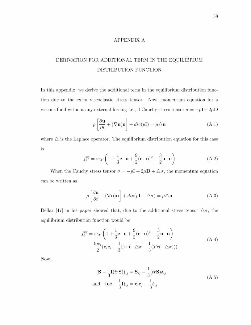
58

APPENDIX A

DERIVATION FOR ADDITIONAL TERM IN THE EQUILIBRIUM

DISTRIBUTION FUNCTION

In this appendix, we derive the additional term in the equilibrium distribution func-

tion due to the extra viscoelastic stress tensor. Now, momentum equation for a

viscous fluid without any external forcing i.e., if Cauchy stress tensor σ = −pI+2µD

ρ

[∂u

∂t+ (∇u)u

]+ div(pI) = µ4u (A.1)

where 4 is the Laplace operator. The equilibrium distribution equation for this case

is

f eqi = wiρ

(1 +

1

3e · u +

9

2(e · u)2 − 3

2u · u

)(A.2)

When the Cauchy stress tensor σ = −pI + 2µD +4σ, the momentum equation

can be written as

ρ

[∂u

∂t+ (∇u)u

]+ div(pI−4σ) = µ4u (A.3)

Dellar [47] in his paper showed that, due to the additional stress tensor 4σ, the

equilibrium distribution function would be

f eqi = wiρ

(1 +

1

3e · u +

9

2(e · u)2 − 3

2u · u

)− 9wi

2(eiei −

1

3I) : (−4σ − 1

3(Tr(−4σ)))

(A.4)

Now,

(S− 1

3I(trS))ij = Sij −

1

3(trS)δij

and (ee− 1

3I)ij = eiej −

1

3δij

(A.5)

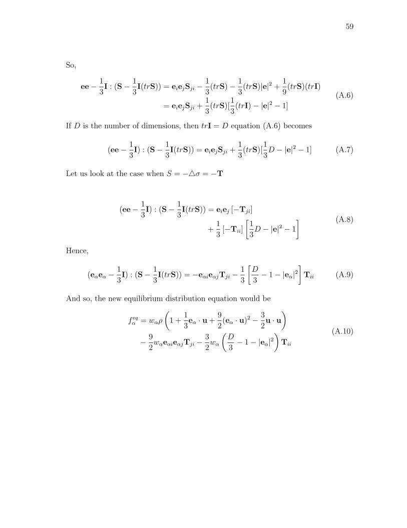
59

So,

ee− 1

3I : (S− 1

3I(trS)) = eiejSji −

1

3(trS)− 1

3(trS)|e|2 +

1

9(trS)(trI)

= eiejSji +1

3(trS)[

1

3(trI)− |e|2 − 1]

(A.6)

If D is the number of dimensions, then trI = D equation (A.6) becomes

(ee− 1

3I) : (S− 1

3I(trS)) = eiejSji +

1

3(trS)[

1

3D − |e|2 − 1] (A.7)

Let us look at the case when S = −4σ = −T

(ee− 1

3I) : (S− 1

3I(trS)) = eiej [−Tji]

+1

3[−Tii]

[1

3D − |e|2 − 1

] (A.8)

Hence,

(eαeα −1

3I) : (S− 1

3I(trS)) = −eαieαjTji −

1

3

[D

3− 1− |eα|2

]Tii (A.9)

And so, the new equilibrium distribution equation would be

f eqα = wαρ

(1 +

1

3eα · u +

9

2(eα · u)2 − 3

2u · u

)− 9

2wαeαieαjTji −

3

2wα

(D

3− 1− |eα|2

)Tii

(A.10)

60

VITA

Satish Karra

Department of Mechanical Engineering, Texas A&M University,

College Station, TX – 77840

EDUCATION

May ’07: M.S Mechanical Engineering, Texas A&M University, College Station, TX.

May ’05: B.Tech Mechanical Engineering, Indian Institute of Technology Madras,

India.

EXPERIENCE

Spring ’07: Graduate Assistant Teaching, Texas A&M University, College Station,

TX.

Fall ’06: Graduate Assistant Research, Texas A&M University, College Station, TX.

Fall ’05–Summer’06: Graduate Assistant Teaching, Texas A&M University, College

Station, TX.