Embed Size (px)
Citation preview
1
Modeling Economic Consequences
of Supply Chain Disruptions
Thomas G. Schmitt Michael G. Foster School of Business
University of Washington Business School Box 353200
Seattle, WA 98195-3200 [email protected]
Sanjay Kumar Black School of Business
Pennsylvania State University - Erie 5101 Jordan Rd
Erie PA 16563- 1400 [email protected]
Kathryn E. Stecke
School of Management The University of Texas at Dallas SM 40, 800 West Campbell Road
Richardson, TX 75080-3021 [email protected]
Fred W. Glover
OptTek Systems, Inc. 2241 17th Street
Boulder, Colorado 80302 [email protected]
Mark A. Ehlen
Sandia National Laboratories P.O. Box 5800
Albuquerque, NM 87185-1138 [email protected]

2
Modeling Economic Consequences of Supply Chain Disruptions
ABSTRACT
Supply chains often experience significant economic disruptions, as in the case of facility
breakdowns, transportation mishaps, natural calamities, and terrorist attacks. We collaborated in
a study of such disruptive events as part of an initiative by Sandia National Laboratories. We
conducted case studies of three electronics firms and their suppliers to explore underlying
aspects of the supply chain structure and complexity, type and length of disruptions, and
mitigation approaches currently in use. We identified three vital metrics (system inventory,
system expediting, and service level at the final echelon in the supply chain) as drivers of
performance. Simulation experiments we ran disclosed four key findings: (1) a cost function
based on these vital metrics can be quite ill-behaved, warranting the use of metaheuristics
capable of looking beyond local optima, (2) genetic search over inventory system parameters
yields better solution quality than unimodal search, (3) variability induced by disruptions can
amplify in a supply chain, and severely affect service levels and system inventory for long
periods, and (4) order expediting, often used to mitigate disruptions, can also trigger bullwhip
effects, and hurt rather than help overall performance.
In sum, while there is merit in the popular notion that increased information and
flexibility are generally desirable, our study discloses that these factors also have significant
attendant dangers, making it easy to overreact.
INTRODUCTION
Resilience to disruptions is a critical issue in supply chain management. Disruptions can have
many sources and affect many supply chain activities. The causes range from natural (e.g.,
Hurricane Katrina, SARS pandemic) to accidental (Minneapolis I-35W bridge collapse, 2009
3
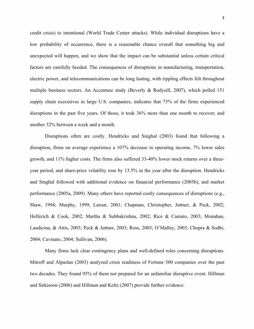
credit crisis) to intentional (World Trade Center attacks). While individual disruptions have a
low probability of occurrence, there is a reasonable chance overall that something big and
unexpected will happen, and we show that the impact can be substantial unless certain critical
factors are carefully heeded. The consequences of disruptions in manufacturing, transportation,
electric power, and telecommunications can be long lasting, with rippling effects felt throughout
multiple business sectors. An Accenture study (Beverly & Rodysill, 2007), which polled 151
supply chain executives in large U.S. companies, indicates that 73% of the firms experienced
disruptions in the past five years. Of those, it took 36% more than one month to recover; and
another 32% between a week and a month.
Disruptions often are costly. Hendricks and Singhal (2003) found that following a
disruption, firms on average experience a 107% decrease in operating income, 7% lower sales
growth, and 11% higher costs. The firms also suffered 33-40% lower stock returns over a three-
year period, and share-price volatility rose by 13.5% in the year after the disruption. Hendricks
and Singhal followed with additional evidence on financial performance (2005b), and market
performance (2005a, 2009). Many others have reported costly consequences of disruptions (e.g.,
Shaw, 1994; Murphy, 1999; Latour, 2001; Chapman, Christopher, Juttner, & Peck, 2002;
Helferich & Cook, 2002; Martha & Subbakrishna, 2002; Rice & Caniato, 2003; Monahan,
Laudicina, & Attis, 2003; Peck & Juttner, 2003; Ross, 2003; O’Malley, 2003; Chopra & Sodhi,
2004; Cavinato, 2004; Sullivan, 2006).
Many firms lack clear contingency plans and well-defined roles concerning disruptions.
Mitroff and Alpaslan (2003) analyzed crisis readiness of Fortune 500 companies over the past
two decades. They found 95% of them not prepared for an unfamiliar disruptive event. Hillman
and Sirkisoon (2006) and Hillman and Keltz (2007) provide further evidence.
4
Sandia National Laboratories, whose research provides the underpinning of our study,
has responded to such contemporary concerns by developing a macro-economic simulation
model of industrial activity. Our role was to guide the modeling of supply chain behavior. The
paper is organized as follows. We review the state-of-the-art in operations management and
economics related to our concerns. Then, we pursue a set of key research questions, whose
answers we glean from case studies and simulation experiments. We propose a four echelon
assembly structure as a baseline in further research by Sandia and others. The results we report
as well as subsequent ones by Sandia (Appendix A) focus on issues of response and recovery
rather than prevention. Our simulation results confirm that disruptions may have long-lasting,
rippling, costly consequences within a supply chain, and that expediting efforts may hinder
rather than help system recovery. We also find that a system cost function can be quite ill-
behaved, even in the absence of disruptions and expediting, and that conventional solution
approaches, which assume convex or unimodal behavior, may be inappropriate for real-world
supply chains.
BRIDGING MACROECONOMIC AND OPERATIONAL DECISION-MAKING
Sandia approached us with an intriguing question: How to model the macroeconomic impact of a
major disruptive event on industrial behavior in a region? Empirical findings indicate that
specific high-impact disruptions are improbable with distributions inexorably hard to quantify.
We also found evidence in the literature and case studies we conducted that firms commonly use
inventory buffering and expediting to mitigate disruptions. For the interested reader, we offer an
extensive review in Appendix B, which positions our work in the literature on disruptions,
expediting, bullwhip effects, and simulation methodology.
5
We consider more complex supply chain structures, order interactions and mitigation
tactics than we found in the literature, in part because of a different research mission. In addition
to contributing to theory and practice in operations management, another objective was to guide
the development of certain aspects of Sandia’s macroeconomic model of regional commerce.
Rather than present explanatory findings on a tightly defined problem, we explore a series of
interrelated research questions using controlled experiments. We were more interested in
exploring elements of reality than tractability.
With a sense of urgency, a group of economists within Sandia embarked on a project to
develop a large scale simulation to assess the regional economic impact of disruptions in critical
infrastructure on U.S. manufacturing firms and their supply chains. They wished to study
vulnerabilities in complex, realistic operating environments, and gain insights about mitigation
strategies. The need for managerial relevance implied fresh methodology capable of relaxing
traditional economic assumptions of aggregation, substitutability, and well behaved performance
of supply and demand. Aggregation is sometimes inappropriate because it tends to cancel valid
cascading effects of variability. While resource substitution may be fitting to mitigate natural
disasters and accidents, it may not be an option in the event of intentional terrorist acts. For
example, Sheffi (2006) suggested that the U.S. Government may respond to an event, such as
uncovering a dirty bomb at one seaport of entry, by closing all seaports for a lengthy period.
Sandia began to develop an agent model capable of simulating the discrete events of
millions of entwined enterprises within regional supply chains, and using enormous computing
power, trace the corresponding economic behavior (Appendix A). They chose the Pacific
Northwest as an initial test site, and we were one of three groups to assist. The others were:
6
Argone National Laboratories to model power generation and distribution, and Lucent
Technologies to cover telecommunications.
Our role was to help Sandia span boundaries in this interdisciplinary effort by conducting
exploratory research into multi-echelon inventory systems. We focused on the ordering systems
across firms in supply chains, which link the procurement, production, distribution, and
transportation activities.
Our field and simulation research summarized here assisted Sandia’s development by
characterizing agent firm structures and inter-relationships, defining model variables and key
performance drivers, hypothesizing critical aspects of supply chain behavior, and validating non-
linear search methodology of parameters. We posited seven interrelated research questions:
1) What is a reasonable baseline for the supply chain structure?
2) What baseline inventory logic reflects sufficiently realistic conditions in a supply chain?
3) Which performance metrics drive the economics in the supply chain?
4) What happens to supply chain system performance in the presence of a disruption?
5) How does expediting affect system performance?
6) How well-behaved is system performance -- should analytics or heuristics be applied in
system ordering?
7) How do genetic and line search compare in solution effectiveness and efficiency?
By addressing these as key modeling issues, we provide insights to Sandia in construction of
their macro-economic model, and offer guidance for future operations management research on
supply chain disruptions.
KEY MODELING ISSUES
We are interested in a supply chain structure that offers enough complexity to reflect a realistic
supply chain composition, yet small enough to control the environment in our experiments as
well as Sandia’s model. To address the key modeling issues, we considered the supply chain
7
literature, conducted case studies in the Pacific Northwest (Sandia’s initial region of interest),
and performed a series of simulation experiments.
Key Issue 1) A Reasonable Baseline for the Supply Chain Structure
Most surveys on disruptions involve large firms. In support of Sandia’s effort, however, we
targeted small and medium-sized manufacturing firms in the Northwest, related supply and
demand activities elsewhere in the U.S. and over-seas, and corresponding transportation
connections. The case firms we selected employ between 250 and 500 workers in a
predominantly small-firm regional economy. Of manufacturing companies in the Northwest,
over 98% employ less than 500 employees (U.S. Census Bureau, 2008). While small in size
individually, these firms drive much of the region’s economic growth in employment, profit, and
demand for non-durables and services. This manufacturing sector represents 20 percent of
overall output in the Washington State economy, and is forecast as the fastest growing sector
over the next decade (REMI, 2007).
Small firms also tend to be more vulnerable economically to disruptions than their larger
counterparts. Because of limited cash reserves and working capital, small firms are more likely
to fail in the event of disruptions. Many do not have the resources to prepare for prevention,
response and recovery from major disruptions. For example, the Institute for Business and Home
Safety (2005) found that after Hurricane Floyd, 30% of impacted small firms never re-opened,
and another 20% closed after two years.
Economic behavior in the Northwest covers many industries and activities, but for our
part, we focused on case studies of electronics companies for three reasons. First, electronics are
important to the functioning of our society. Logic chips can be found in products ranging from
automobiles to electric toothbrushes.
8
Second, electronics assembly is susceptible to disruption because of the complexity of
assembly and component supply. We found in three case studies that electronics assembly
requires from 70 to 700 components to make one product type, and a shortage of any one delays
the completion and sale of the product. Even under stable conditions, extremely high buffer
levels are needed to prevent such delays. For example, if a company maintains a 99% service
level (amount supplied/amount demanded) for each component, the probability of having, say,
700 components available at any point of time is 700.99 , roughly equal to 0.009%.
Third, electronics supply chains involve global, multinational interests that broaden the
exposure to disruption. We found in the case studies that most electronic components are
internationally sourced. Additionally, some of the electronic assemblies are embedded into larger
systems made by such customers as Boeing and Honeywell, who in turn, export many products.
Electronics companies in the Northwest make products ranging from consumer
appliances to devices used by original equipment manufacturers (OEMs). To gain insights into
supply chain behavior in that industry, we interviewed personnel from three representative
electronics firms and some of their suppliers. We disguise identities of the three because their
management considers certain information proprietary and security-sensitive. We label the three
as firms INT, ABC, and XYZ, and summarize the cases in Table 1 with details in (“Case Studies
of Electronics Companies,” an enclosed working paper to be cited as an online reference).
[Table 1 here]
The supply chains in all three support a minimum of four echelons and component
assembly. Each echelon requires activity and storage. Figure 1 shows our rudimentary supply
chain model. At Echelon 1, products are demanded and shipped to a local or out-of-town
customer, which might be an OEM manufacturer, distributor, or retailer. Echelon 2 represents
assembly of components A and B into finished goods. In Stages 3A and 3B of Echelon 3,
9
suppliers (internal, local, out-of-town) transport the parts, or fabricate prior to transport. Stages
4A and 4B represent transportation activities of domestic or overseas distributors. The figure also
displays lead time parameters in days -- lead times (LTs) under normal operating conditions, and
expedited lead times (ELTs). These reflect the times of production and delivery, and are based
on the literature and observations in our case firms. We review the model logic in the next
section, with details in Appendix C.
[Figure 1 here]
We cannot generalize beyond electronics, but this four echelon structure with assembly
seems reasonable as a baseline for a manufacturing supply chain in our model as well as
Sandia’s. Among supporters of a minimum of four echelons, Juneja and Rajamani (2003) cite an
electronics supply chain with assembly that includes Selectron (supplier), Matsushita
(manufacturer), Panasonic (distributor), and Best Buy (retail customer). Across industries, most
simulation research on bullwhip effects covers four echelons (Appendix B). Additionally,
Swaminathan et al. (1997) propose multiple echelons and assembly to motivate the use of agent
modeling. We felt comfortable as well including assembly of at least two components. Whether
at home, in an office, in a vehicle, or in a factory, one would likely encounter products
comprised of two or more components.
Key Issue 2) Inventory Logic
We addressed one aspect of Sandia’s simulation model, the supply chain ordering systems,
which regulate the goods flows and inventories across echelons. Ordering systems serve as a
fundamental means of linking activities between companies in a supply chain.
Our interviews revealed that operating managers within the case firms and their suppliers
seldom share point-of-sale data. Most were familiar with features of the Beer Game, and claimed
that their processes encountered the full effects of demand amplification. There was strong
10
consensus that the way to model reality across firms is through local forecasting and buffering.
They also rescheduled frequently (expediting some orders, and postponing others) without the
benefit of shared data across firms. We recognize however, the existence of progressive supply
chains that plan more holistically (e.g., Brown, Schmitt, Schonberger, & Dennis, 2004; Ferdows,
Lewis, & Machuca, 2004; Li, Shaw, Sikora, Tan, & Yang, 2006).
We assume stationary, autocorrelated demand at Echelon 1. Each echelon/stage observes
only the demand it receives from its immediate stage customer. Using historical demand
observed from the immediate customer, we forecast at every stage the mean and variance of
demand using single exponential smoothing, a method used by many companies (Snyder,
Koehler, Hyndman & Ord, 2004; Gardner, 1985; Makridakis & Hibon, 2000).
The demand and variance estimates are applied, along with a service-level parameter, in a
single-stage order-up-to formula to calculate the replenishment order quantity. Replenishment
orders at one echelon/stage shown in Figure 1 become the demand at the preceding stage.
Inventory balance equations link each stage in a periodic (daily) review system. Each stage
follows the FIFO logic each day: (a) launch a replenishment order if necessary using an order-
up-to system, (b) withdraw this day’s demand from available inventory to initiate shipment to
the customer, (c) receive goods from the previous stage into inventory, and (d) update the
inventory, or backorder quantity where backorders are permitted.
If demand at the succeeding stage is more than the available inventory, we assume a
partial shipment. The rest is lost at Echelon 1, and backordered at Echelons 2, 3, and 4. (Other
approaches to shortages are applied as well in practice -- Sodhi, 2005.) Prior to assembly at
Echelon 2, inventory of the two component types is maintained, and orders for each are placed if
11
warranted. The quantity of an assembly order cannot exceed the minimum available inventory of
the two components.
The parameters we use in demand generation, forecasting and inventory control are
presented in Appendix C. The order logic assumes periodic review with no setup or order cost,
infinite production rates, fixed lead times, and i.i.d. demands. While suitability of order-up-to
policies is by no means assured for our system, this logic is the most robust and applicable of
those available. Such a policy is common in practice and has been studied extensively in the
literature. Nahmias (2008) and Axsater (2000) provide details about order-up-to systems, which
afford optimality for base-stock policies under certain assumptions about the supply chain
structure, shortages, order cost, and demand distributions. Recent papers have found base-stock
policies optimal over a variety of unimodal risk-neutral and risk-averse objectives in single-item,
single stage systems with multi-period finite horizons and no order cost (e.g., Marinez-de-
Albeniz & Simchi-Levi, 2006; Chen et al., 2007; Huh et al., 2009). We recommended to Sandia
the aforementioned inventory logic for their macroeconomic model.
Key Issue 3) Performance Metrics
Three operational metrics drive important economic effects in the case supply chains. The first is
the service level experienced by customers of electronics firms at the final supply chain echelon.
At the final echelon, customers such as retailers and OEMs may have choices, and shortages may
be lost to the firm (as in cases INT and ABC). Others, e.g., some OEMs, may have contractual
arrangements that might instead specify backorders (INT and XYZ). The opportunity costs of
shortages from either lost sales or backorders that reach the final echelon can be severe, with loss
of future business at stake. For example, late delivery of avionics to Boeing Commercial, an
OEM customer, may in turn cause late delivery of an aircraft. This would result in loss of interest
12
on delayed revenue receipts of hundreds of millions of dollars, diminished revenue arising from
contractual penalties, and loss of goodwill with the airlines.
Firms at intermediate echelons typically have long term relationships with customers that
call for backordering non-commodity items (Sodhi, 2005). Countermeasures such as expediting
and inventory positioning enable some of this late work to catch up in subsequent stages.
Nevertheless, system expediting, the second metric, introduces significant premiums for
transportation and production that drain profit margins throughout the supply chain.
The third metric, system inventory, also drains profit margins. Well-positioned inventory,
however, provides a safety net against disruptions, and can decrease shortages and expediting.
We chose total supply chain inventory as a metric because without accountability, inventory in
motion or at rest might be shifted elsewhere, and associated costs overlooked.
To further guide Sandia, we conducted simulation runs using the aforementioned model
structure and metrics, and adapted the experimental design accordingly to each of the remaining
Key Issues 4-7. Cost structures varied substantially by firm and item in our case studies. We
addressed this complication in ways which differ by key issue. With Key Issues 4 and 5, we
apply MANOVA across performance metrics, and focus on statistical inferences consistent
among them. With Key Issues 6 and 7, we weight the metrics to represent different cost
structures. An example that demonstrates ill-behaved cost performance is presented in 6, and this
phenomenon, which challenges traditional tractability assumptions, is supported in 7 by
statistical analysis over a variety of cost structures.
Key Issue 4) System Performance with a Disruption
Sandia wished to study the effects of a supply chain disruption on regional economics.
Management within all three case supply chains indicated that “time of a disruption” becomes
13
the critical factor, and expressed concerns about response and recovery. They had encountered
disruptions of fire, weather disasters, worker strikes, port lockouts, supply shortages, power
failures, telecommunication failures, transportation breakdowns, and machine breakdowns. Loss
of a sole-source supplier introduces delays of up to two years to find and procure alternate
materials (as in the case of INT – Table 1). A disruption in transportation of commodity
components, with replenishment by sea, might involve as much as a 90-day delay (as with
Supplier 5 in “Case Studies of Electronics Companies,” an enclosed working paper to be cited as
an online reference). Loss of electric power or telecommunications would quickly stop activities
in every firm in the area during the length of the disruption, although essential
telecommunication transactions might be handled by cellular telephone, if the networks are not
overloaded. Management of the case firms agreed that traditional preventative measures such as
fencing, guards and lighting are insufficient, and that contingency planning deserves to be
elevated in importance within their organizations and across firms. It was expressed that quality
information is sparse during a crisis, even in the most progressive of supply chains. One would
not likely know how the other customers and suppliers will behave during a disruption, and when
the disruption will end.
Consequently, we chose to introduce a generic shock (time delay) to represent many
types of disruptions that occur in practice, and to limit information sharing across echelons. For
our experiments the review period is one day. After an initialization period of 1000 days, we
induce a 20-day disruption, and compare performance thereafter with the base case (without
expediting and disruptions). We explore issues of simulation steady state and statistical
independence in Appendix C.
14
We consider disruptions at each end of the supply chain: Echelon 1 (shipment to
customers), and Echelon 4/Stage A (supply by a parts distributor). During each disruption, the
facility at the affected echelon receives shipments or orders in-route before the start of the
disruption, but stops all other operations. It cannot place orders, produce orders, or make
shipments.
For Key Issue 4, we observe the performance on a day-by-day basis over 100-day time
blocks, replicate the experiments 100 times, and compare performance between the disrupted and
base cases. A time block covers five months in a 240-working day year. Our MANOVA design
has two fixed factors: time block, and location of disruption. We do not mitigate with expediting,
and observe the service-level and system-inventory metrics as dependent variables.
We find that values from each metric are drawn from different distributions, according to
Pillai's Trace, Wilks' Lambda, Hotelling's Trace, and Roy's Largest Root statistics at the .01 level
(Arbuckle, 2005). Results for the two metrics are summarized in Figure 2. Each point in the
graphs depicts the mean value over an indicated five-month time block.
[Figure 2 here]
Waller-Duncan multiple-range post-hoc tests disclose that regardless of the location of
disruption, service level is significantly different between the disrupted state and base-case state
over the first two time blocks (10 months). In the final eight time blocks, there is no significant
difference among the means and zero. All of these results hold at the .01 and .05 levels.
System inventory is significantly different over the first five time blocks (25 months)
with both disrupted locations. In the final five time blocks, there is no significant difference
among the means and zero. Clearly, the effects of disruptions on the two performance metrics
last for a long time. There are severe decreases in service level for more than a year. Additional

15
system inventory over the base case exceeds ten weeks of demand for more than two years after
a disruption at Echelon 1.
We performed additional analyses comparing disruptions at Echelons 1 and 4 (contrasts
between means in left and right graphs). The MANOVA contrasts at the .01 level indicate
significantly worse service levels at Echelon 1 than 4 over the first five months, as well as
increased system inventory (more than twice the amount) in months six through 25. We observe
a strong whipping effect across echelons, especially with a disruption at Echelon 1. This is in
contrast to findings by Wu and Chen (2009) who noted that regardless of source in a two stage
system, larger fluctuations occur closer to the disruption and dampen when propagating away.
We attribute this to differences in our model of more than two echelons, our ordering system, our
forecasting system, the presence of lead times, and the limited information sharing. Recognition
of a disruption at Echelon 1 is transmitted to other firms as a function of the smoothing
parameter α, service level parameter, and echelon lead times in our system. Even with small α
values, the forecasted demand at subsequent echelons drops relatively fast, which reduces the
order-up-to levels and order quantities. This amplifies as the variability propagates across
echelons from Echelon 1 in accord with lead time offsets, a finding also observed by Chen et al.
(2000a).
By contrast, a disrupted facility at Echelon 4 immediately suspends production and
shipment to Echelon 3, but the interruption in supply goes unnoticed in our system, i.e., until
shortages eventually appear as lost sales at Echelon 1. Beforehand, shifts occur from inventories
to backorders at Echelons 4, 3 and 2, but the pipeline totals remain stable, and so do the order-
up-to levels, demand forecasts and order quantities.
16
Our experimentation sheds light on the relevance of Key Issue 4, and highlights the
importance of studying the effects of disruptions at different stages in the supply chain. This led
us to recommend that Sandia consider disruptions at various stages and between stages.
Key Issue 5) System Performance under Expediting
Firms within all three case supply chains frequently use expediting to avoid shortages.
Depending on the echelon, the percentage of orders expedited ranges from 5-20%, with a
premium cost per unit ranging from 10-50%. Bradley (1997) provides additional motivation for
expediting within the electronics industry. Expediting is typically accomplished with faster
transportation, or production adjustments such as overtime, additional shifts, part-time help,
alternate routing and outsourcing.
Following prior practice and research, we apply two triggers to expedite lead times as
orders are launched, and experimented with a range of parameters for each type of trigger to
achieve an expediting frequency we observed in the case studies. The first is activated when the
quantity throughout the stage pipeline (on-order plus on-hand inventory) falls below the expected
lead time demand (Fukuda, 1964; Whitmore & Saunders, 1977; Groenevelt & Rudi, 2003;
Veeraraghavan & Wolf, 2008). The second trigger is activated when the on-hand inventory falls
below a demand-based target (Appendix C). Beyer and Ward (2002) observed that Hewlett
Packard’s supply network applies this second type of trigger to expedite via air transport.
We compare performance results of the base case (without expediting and disruption)
with expediting (no disruption). If the expediting option is enabled, we permit expediting at all
echelons, with order crossover a possibility. We replicate 100 times and apply all three
performance metrics (final-echelon service level, system inventory, and system expediting) as
dependent variables.
17
Values from the three metrics are drawn from different distributions at the .01 level in the
MANOVA. We also observe significant performance differences at the .01 level between the
base and expediting cases for each metric. While significant, however, the relative performance
differences raise issues about the value of expediting. Shortages improve with expediting by only
0.18 units per day on average demand of 111 units, while total system inventory increases by an
average of 787 units per day (almost eight days of average demand). System inventory increases
so much because expediting increases the variability in order quantity and frequency, and this
variability is amplified elsewhere in the supply chain.
According to the personnel we interviewed, expediting offers a first line of defense
against shortages, but our findings raise questions about the value of this practice as a mitigation
approach of choice. We are not the first to raise the concern. Even before bullwhip effects were
recognized, the practice of expediting was challenged because of nervousness it induces in MRP
systems (e.g., citations in Schmitt, 1984). In addition, expediting, while considered necessary
(Bradley, 1997; Cohen et al., 2003), is usually expensive (Arslan, Ayhan, & Olsen, 2001;
Groenevelt & Rudi, 2003). Beyer and Ward (2002) observed that expediting by air in HP’s
supply chain costs up to five times more than standard shipment by sea. In the case firms, we
found that expediting was quite expensive as well.
Regardless of the evidence, however, we do not expect firms to discontinue the practice
of expediting. For example, it would be difficult to convince managers of an electronics firm not
to expedite one component, when the remaining 700 needed for assembly and sale of a finished
product are available. However, practitioner behavior might be influenced by research that finds
merit in the application of certain types of expediting at specific supply chain stages, or between

18
stages. This future work by Sandia and others should consider collectively the effects of
expediting and bullwhip.
Key Issue 6) System Performance and Applicability of Analytics and Heuristics
Traditionally, researchers offering analytics or heuristics have been careful in claiming utility
only within their system assumptions. Base-stock policies have been shown optimal for
stationary stochastic demand in simple supply chains (Axsater, 2000; Porteus, 2002). Without
claiming optimality, some have used order-up-to and other well known policies in simple supply
chains in the presence of supply or demand disruptions (Chao, 1987; Gupta, 1996; Arreola-Risa
& DeCroix, 1998; Snyder et al., 2006; Lewis et al., 2008).
In this section, we observe non-unimodal total cost behavior within a range of stage
order-up-to levels under conditions of no expediting and no disruptions. To make a case, we
choose a holding cost of $1/unit/day, a backorder cost of $2/unit/day (at Echelons 2, 3, and 4), a
lost-sales cost of $3/unit (at Echelon 1), and a stage production/transportation cost of $1/unit. We
present here the notable erratic behavior for this case, and in the next section, report summary
statistics over a variety of costs.
[Figure 3 here]
Figure 3 shows plots of the simulation results of total cost over various stage order-up-to
levels for this example. The two graphs to the left focus solely on behavior at Echelon 1, while
the ones to the right show interactions between Echelon 1 and Echelon 2.
The graphs on the left show total cost values for discrete order-up-to levels at Echelon 1,
while allowing the other three echelons to derive order-up-to levels from stage demand forecasts.
The top left graph displays total cost performance versus Echelon 1 order-up-to levels over the
range [1, 2000]. Clearly, the local optima vary considerably in value, e.g., one yields a total cost
6.95 times larger than the lowest observed total cost value, given the starting point. The bottom

19
left graph depicts a finer grain relationship over the range [1000, 1530]. It highlights the striking
volatility of the cost function.
The graphs on the right of Figure 3 show the interactive behavior between the first two
echelons, depicting total supply chain cost while varying Echelon 1 order-up-to levels for
prescribed Echelon 2 levels. In this set of experiments, Echelons 3 and 4 derive order-up-to
levels from stage demand forecasts. The course and fine grain representations at the top and
bottom right, respectively, generalize the previous observations solely about Echelon 1. Clearly,
computationally-efficient iterative line searches or analytic searches could derive very poor
solutions in this operating scenario, depending on the starting point.
There are multiple ways to confirm concerns about ill-structured performance behavior
and inappropriateness of exact approaches. These involve violations of Kuhn-Tucker conditions,
or alternatively, properties of derivatives. We chose another way, the presentation of a counter
example, one where an exact approach would yield higher total cost. Existence of such a counter
example, with differences of any magnitude, is sufficient to obviate generality of exact analytical
approaches that assume unimodality. Nevertheless, we consider in the next section the relative
efficacy of a unimodal search method over a wide variety of cost structures.
Key Issue 7) Genetic Search versus Line Search
With insight from the preceding key issue, we examine the modality of the objective function
surface across different cost settings. Sandia programmed a general genetic search (GA) function
to “jump over” local optima. We conducted experiments to evaluate Sandia’s GA approach. We
restrict the search for cost-effective order-up-to quantities to Echelon 1, while allowing demand
forecasts to guide decision making at other echelons. The GA utility represents candidate
20
solutions as binary numbers. Crossover and mutation operators are used to overcome local
minima. For details, see Goldberg (1989).
We consider line search (LS) as a basis for procedural comparison and modality
concerns. LS ensures optimality only when the objective function is unimodal. In our problem
setting, a LS approach that increments upwards from an order quantity of 0 to find a local optima
typically yields much higher costs than GA. To facilitate a reasonably fair comparison, our
adaptation of LS begins with an order-up-to quantity equal to the mean lead time demand at
Echelon 1 and searches each way in the neighborhood (upward first) until we encounter local
optima. This initialization adaptation resulted in much better LS solutions in pilot experiments.
[Table 2 here]
To represent a wide variety of operating conditions, we selected a range of cost
parameters as presented in Table 2. We considered findings from the literature in the context of
our research objectives. Relative costs depend on the type of product, industry, and supply chain,
among other factors. Cohen et al. (2003) observed that with short life cycles and obsolescence in
the semiconductor industry, the cost of losing a sale is about twice the cost of backlogging.
Faaland et al. (2004) experimented with lost-sales costs in a single-echelon ranging from 62 to
500 times the periodic inventory holding cost, shortage values much higher than the ones we
chose. Their parameters were based on a cross-industry survey by Boer and Jeter (1993). Our
motivation in the choice of relatively low shortage costs is to compare GA and LS under modest
conditions. We observed in pilot experiments that larger shortage costs relative to inventory
carrying costs further exaggerated differences between GA and LS.
[Table 3 here]
Table 3 shows the cost savings under various cost scenarios. The percentage
improvements represent averages over 100 replications for each of the 16 cost combinations.
21
The superiority of GA over LS at Echelon 1 holds at the 0.005 level using student-T tests. GA as
compared with LS yields overall cost savings greater than 16%, and in one scenario by more
than 30%. Less effective starting solutions for LS would have enabled greater savings.
In single-stage stationary systems, even with deterministic demand, tractability has not
been established when shortages are lost (e.g., Karlin & Scarf, 1958; Nahmias, 1979; Donselaar
et al., 1996; Metters 1997; Ketzenberg et al., 2000; Janakiraman & Roundy, 2004). Others have
acknowledged, but discounted this phenomenon by asserting that the total cost surface is
relatively flat in regions around the global minimum. We question this conventional wisdom by
showing how far off the local optima may be under a broad spectrum of cost parameters. Recent
papers on disruptions, expediting and bullwhip effects have expressed similar concerns, and we
summarize in Appendix B some of their arguments as well as relevant simulation results.
Genetic Search yielded significantly better costs at the expense of computation time in
our experiments. On a laptop, the time per run for GA was about 14 hours, and our adaptation of
LS averaged about 10 minutes. While the computation time for GA may be acceptable for
Sandia with its fast complex of computers, we recognize an opportunity in future work to adapt
standard GA utilities to special properties of this problem setting.
CONCLUSIONS AND FUTURE DIRECTIONS
Disruptions can have many sources covering the gamut from natural to accidental to intentional.
Regardless of cause, disruptions can have long-lasting, widespread, and costly effects on supply
chains. We describe aspects of a stream of research to assess the economic impact of supply
chain disruptions. The overarching research mission of our sponsor, Sandia National
Laboratories, is to develop a simulation model that depicts regional economic behavior after a
disruptive event. Simulation is intended to augment existing analytical and statistical models
22
whose utility may depend on the validity of inherent simplifying assumptions. Optimization
models routinely assume aggregation of demand and supply data, substitutability of supply
options, independent and steady-state behavior of underlying stochastic distributions,
optimization over well-behaved objective functions, and simple supply chain structures (Chen,
Sim, Simchi-Levi, & Sun, 2007 and citations). Sandia’s concern was that with such high stakes
in security matters, entities within the U.S. government and private sectors cannot afford to wait
for researchers to overcome the substantial challenges of relaxing these simplifying assumptions
in the optimization models.
Sandia’s agent simulation has the capability to incorporate supply chain networks with a
million or more firms and supporting infrastructure. The first project for the system has been to
address the Pacific Northwest region. We concentrate on one aspect of this effort on how to
model business activity within supply chains. It is anticipated that these insights will be useful in
other research as well.
We conducted case studies of three electronics firms in the region, and drew from the
cases to offer a fundamental set of design requirements, performance drivers, and research
questions. Sandia may not need to represent entire supply chains, but if electronics
manufacturing is representative, their model should include at least:
• Four echelons per supply chain,
• An echelon with assembly,
• Bullwhip effects facilitated by a multi-echelon inventory system with local planning,
• Shortages along the supply chain in the form of backorders and lost sales,
• Capability to expedite at all stages,
• Three metrics as performance drivers (service level at the final echelon, system
expediting, and system inventory), and
• Disruptions in the form of time delays at various stages in the supply chain.
23
To guide Sandia’s experimentation, we followed the aforementioned model design issues
with research questions, whose answers were driven by simulation results. One important finding
was that the system cost function can be quite ill-behaved in a four-echelon supply chain, even in
the absence of disruptions and expediting. We reveal a weakness of analytical optimization
approaches in the present setting by providing a counter example where these methods would be
unable to obtain satisfactory solutions. This is further supported by statistical evidence over a
wide range of operating conditions. Analytical methods that assume unimodal behavior may be
inappropriate for real-world supply chains.
Another finding confirms that disruptions may have long-lasting, rippling and costly
consequences within the supply chain structure presently considered. We also observe that
standard industry practices of setting order parameters locally and using expediting as mitigation
seem to exacerbate these undesirable effects. In addition, our cases, experimentation and
subsequent observations by Sandia (Appendix A) support the recommendations by Craighead et
al. (2007). They propose simulation analysis and field study as means to verify propositions that
the severity of a disruption is related to time, its location, the structure of the supply chain, and
types of mitigation. We believe as well that additional field study across industries is warranted.
We address disruptions at each end of a four echelon supply chain, but we suggest that an
expanded study may find value in investigating disruptions elsewhere. In support of this,
Sandia’s model has capabilities to explore more fully disruptions in specific areas of network
criticality, i.e., at any supply chain stage, between stages, and in infrastructure shared by firms
within a region (transportation hubs, electric power, and telecommunications). Their model
offers other flexibilities, e.g., parts distributors may have multiple customers. This may enable
demand aggregation and dampening of the demand amplification elsewhere in the supply chain.
24
Our experimental results suggest caution and restraint, however, in how information is
applied. Sharing offers clear advantages in a supply chain, and some authors have addressed this
issue (e.g., Milgrom & Roberts, 1988; Lee et al., 2000; Chatfield, Kim, Harrison, & Hayya,
2004; Sodhi, 2005). As a caveat, information must be discounted considerably to control the
bullwhip effects in our decentralized system. Pilot experimentation indicated a very low
forecasting weight of 0.01 on the most recent local information for the firms in the last echelon,
Echelon 4. While we support the notion that increased information and flexibility to react are
generally desirable, we caution that it is possible to overreact. A disruptive event creates a
critical watershed. The issues are how much weight to place on the news and what to do about it.
Furthermore, with the irregular cost objective surface documented by our results, we
believe future efforts should be directed towards developing efficient and effective search
methods to find local optima close to global cost values. Research is needed to explore the
efficacy of hybrid GA approaches as well as other metaheuristics (Holland, 1992; Corne et al.,
1999; Gen & Cheng, 2000; Kimbrough et al., 2002; Glover & Kochenberger, 2003; Rego, 2005).
Instead of increasing the generation count to further improve solution quality, a better alternative
might be to assign the lead time demand as one starting solution for a GA approach. This might
help solution effectiveness and efficiency as it did with LS in our experiments.
Our findings suggest that consideration of lost sales, multiple echelons and assembly
perturb the stationary behavior that has otherwise been documented in less complex systems,
and that disruptions and expediting exacerbate the situation. Further research is warranted on
dynamic order-up-to policies, with parameters updated periodically, whether the adjustments
are made using adaptive search over demand history, or cost-based search over order-up-to
parameters. This premise is further supported by simulation experiments conducted by Ross et
25
al. (2008) who found instances where a time-varying order-up-to policy is more effective than a
static policy in terms of the total costs of holding, ordering and lost sales. From a practical
perspective, case firms such as those we studied, which employ periodic-review time-phased
order point systems, may be able to incorporate dynamic ordering policies.
Additional insights may also result from research that relaxes some of our simplifying
assumptions. Sandia has already extended our model to include price/demand elasticity
functions, and a diverse customer base for agent firms. Our experiments embraced both normal
and expedited activity lead times, but did not consider capacity interactions that might result
from finite replenishment, setups, and specific capacity adjustments such as overtime, additional
shifts, part-time help, alternate routing and sub-contracting. Non-stationary demand, stochastic
lead times, stochastic failure times, and lead time/demand elasticity represent other realistic
extensions.
However, prior work as well as ours suggests that variability in quantity and timing,
whether from normal operations, disruptions, or expediting, tends to be amplified in supply
chains. It is possible, although unlikely, that extensions, such as those we suggest for future
work, would resolve the tractability issues we observed in a less complex problem setting. The
practical value of our contribution is affirmed in the following feedback from Sandia (2007):
“[This work] demonstrated the importance of careful design in modeling the realities of supply
chain behavior, and provided strong motivation for further simulation development and
experimentation.”
26
REFERENCES
Arbuckle, J. L. (2005). Amos 6.0 User's Guide. Chicago, IL: SPSS Inc.
Arreola-Risa, A., & DeCroix, G. A. (1998). Inventory management under random supply disruptions and partial backorders. Naval Research Logistics, 45(7), 687-703.
Arslan, H., Ayhan, H., & Olsen, T. L. (2001). Analytic models for when and how to expedite in make-to-order systems. IIE Transactions, 33(11), 1019-1030.
Axsater, S. (2000). Inventory Control. Norwell, MA: Kluwer Academic Publishers.
Baganha, M. P., & Cohen, M. A. (1998). The stabilizing effect of inventory in supply chains. Operations Research, 46 (3), 572–583.
Baldor, L. C. (2007). State Bank on 9/11 terrorists’ hit list. The Associated Press, Seattle Post-Intelligencer, March 15.
Berk, E., & Arreola-Risa, A. (1994). Note on future supply uncertainty in EOQ models. Naval Research Logistics, 41(1), 129-132.
Berman, O., Krass, D., & Menezes, M. B. C. (2007). Facility reliability issues in network p median problems: strategic centralization and co-location effects. Operations Research, 55(2), 332-350.
Beverly, R., & Rodysill, J. (2007). Risky business. Outlook Journal, accessed August 14, 2007, http://www.accenture.com/Global/Research_and_Insights/Outlook/By_Issue/Y2007/RiskyBusiness.htm.
Beyer, D., & Ward, J. (2002). Network server supply chain at HP: A case study. In J. Song, & and D. Yao (Eds.), Supply Chain Structures: Coordination, Information and Optimization, Chapter 8, Norwell, MA: Kluwer Academic Publishers.
Boer, G., & Jeter, D. (1993). What’s new about modern manufacturing? Empirical evidence on manufacturing cost changes. Journal of Management Accounting Research, 5, 61-83.
Bowersox, D. J., & Closs, D. J. (1996). Logistics Management: The Integrated Supply Chain Process, New York, NY: McGraw-Hill.
Bradley, J. R. (1997). Managing Assets and Subcontracting Policies. PhD. Dissertation, Stanford University, Stanford, CA.
Brown, K. A., Schmitt, T. G., Schonberger, R. J., & Dennis, S. (2004). QUADRANT homes applies lean/JIT concepts in a project environment. Interfaces, 34(6), 442-450.
27
Brown, R. B. (1963). Smoothing, Forecasting and Prediction. Englewood Cliffs, NJ: Prentice-Hall.
Cavinato, J. L. (2004). Supply chain logistics risks: From the back room to the board room. International Journal of Physical Distribution & Logistics Management, 34(5), 383-387.
Chao, H. P. (1987). Inventory policy in the presence of market disruptions. Operations Research, 35(2), 274-281.
Chapman, P., Christopher, M., Juttner, U., & Peck, H. (2002). Identifying and managing supply chain vulnerability. Logistics and Transport Focus, 4(4), 1-5.
Chatfield, D., Kim, J., Harrison, T., & Hayya, J. (2004). The bullwhip effect – Impact of stochastic lead times, information quality, and information sharing: A simulation study. Production and Operations Management, 13(4), 340-353.
Chen, Y. F., Ryan, J. K., & Simchi-Levi, D. (2000a). The impact of exponential smoothing forecasts on the bullwhip effect. Naval Research Logistics, 47(4), 271-286.
Chen, F., Drezner, Z., Ryan, J. K., & Simchi-Levi, D. (2000b). Quantifying the bullwhip effect in a simple supply chain: The impact of forecasting, lead times and information. Management Science, 46(3), 269-286.
Chen, Li., & Lee, H. L. (2009). Information sharing and order variability control under a generalized demand model. Management Science, 55(5), 781–797.
Chen, X., Sim, M., Simchi-Levi, D., & Sun, P. (2007). Risk aversion in inventory management. Operations Research, 55(5), 828-842.
Chopra, S., & Sodhi, M. S. (2004). Managing risk to avoid supply chain breakdown. Sloan Management Review, 46(1), 63-61.
Closs, D. J., Roath, A. S., Goldsby, T. J., Eckert, J. A., & Swartz, S. M. (1998). An empirical comparision and response-based supply chain strategies. International Journal of Logistics Management, 9(2), 21-34.
Church, R. L., & Scaparra, M. P. (2007). Protecting critical assets: The r-interdiction median problem with fortification, Geographical Analysis, 39(2), 129-146.
Cohen, M., Ho, T., Ren, J., & Terwiesch, C. (2003). Measuring imputed cost in the semiconductor equipment supply chain. Management Science, 49(12), 1653-1670.
Corne, D., Dorigo, M., & Glover, F. (1999). New Ideas in Optimization. New York, NY: McGraw-Hill.
28
Craighead, C. W., Blackhurst, J., Rungtusanatham, J. M., & Handfield, R. B. (2007). The severity of supply chain disruptions: Design characteristics and mitigation capabilities. Decision Sciences, 38(1), 131-156.
Croson, R., & Donohue, K. (2006). Behavioral causes of the bullwhip effect and the observed value of inventory information. Management Science, 52(3), 323-336.
Donselaar, K., Kok, T., & Rutten, W. (1996). Two replenishment strategies for the lost sales inventory model: A comparison. International Journal of Production Economics, 46–47(1), 285–295.
Downes, P. S., Ehlen, M. A., Loose, V. W., Scholand, A. J., & Belasich, D. K. (2005a). Estimating the economic impacts of infrastructure disruptions to the U.S. chlorine supply chain: Simulations using the NISAC agent-based laboratory for economics (N-ABLE™), SAND2005-2031, Sandia National Laboratories.
Downes, P. S., Ehlen, M. A., Loose, V. W., Scholand, A. J., & Belasich, D. K. (2005b). An agent model of agricultural commodity trade: Developing financial market capability within the NISAC agent-based laboratory for economics (N-ABLE™), Sandia National Laboratories.
Downes, P. S., Ehlen, M. A., Loose, V. W., Scholand, A. J., & Belasich, D. K. (2006). Modeling in N-ABLE™, National Infrastructure Simulation & Analysis Center, SAND2006-6586, Sandia National Laboratories.
Eidson, E. D., & Ehlen, M. A. (2005). NISAC Agent-Based Laboratory for Economics (N-ABLE™): Overview of agent and simulation architectures, SAND2005-0263, Sandia National Laboratories.
Faaland, B. H., Schmitt, T. G., & Arreola-Risa, A. (2004). Economic lot scheduling with lost sales and setup times. IIE Transactions, 36(7), 629-640.
Fukuda, Y. (1964). Optimal policy for the inventory problem with negotiable leadtime. Management Science, 10(4), 690-708.
Ferdows, K., Lewis, M. A., & Machuca, A. D. (2004). Rapid-fire fulfillment. Harvard Business Review, 82(11), 104-110.
Gardner, E. S. (1985). Exponential smoothing: The state of the art, Journal of Forecasting, 4, 1-28.
Gen, M., & Cheng, R. (2000). Genetic Algorithms and Engineering Optimization, New York, NY: John Wiley & Sons.
29
Glover, F., & Kochenberger, G. (2003). Handbook of Metaheuristics. Boston, MA: Kluwer Academic Publishers.
Goldberg, D. E. (1989). Genetic Algorithms in Search, Optimization, and Machine Learning, Reading, MA: Addison-Wesley.
Gupta, D. (1996). The (Q, r) inventory system with an unreliable supplier. INFOR, 34(2), 59-76.
Groenevelt, H., & Rudi, N. (2003). A base stock inventory model with possibility of rushing part of order. Working paper, Simon School of Business, University of Rochester, Rochester, NY.
Hadley, G., & Whitin, T. M. (1963). Analysis of Inventory Systems. Engelwood Cliffs, NJ: Prentice Hall.
Helferich, O. K., & Cook, R. L. (2002). Securing the Supply Chain. Lombard, IL: Council of Logistics Management.
Hendricks, K. B., & Singhal, V. R. (2003). The effect of supply chain glitches on shareholder value. Journal of Operations Management, 21(5), 501-522.
Hendricks, K. B., & Singhal, V. R. (2005a). An empirical analysis of the effect of supply chain disruptions on long-run stock price performance and equity risk of the firm. Production and Operations Management, 14(1), 35-52.
Hendricks, K. B., & Singhal, V. R. (2005b). Association between supply chain glitches and operating performance. Management Science, 51(5), 695-711.
Hendricks, K. B., & Singhal, V. R. (2009). Demand-supply mismatches and stock market reaction: evidence from excess inventory announcements. Forthcoming in Manufacturing and Service Operations Management.
Hillman, M., & Keltz, H. (2007). Managing risk in the supply chain—A quantitative study, accessed May 2009, available at http://www.amrresearch.com/Content/DisplayPDF.aspx?compURI=tcm:7-13798.
Hillman, M., & Sirkisoon, F. (2006). Pandemic readiness study. Report, AMR Research, http://www.amrresearch.com/research/reports/images/2006/0605AMR-A-19413.pdf.
Holland, J. H. (1992). Adaptation in Natural and Artificial Systems. Cambridge, MA: MIT Press.
Huggins, E. L., & Olsen, T. L. (2005). Inventory control with generalized expediting. Working paper, School of Business Administration, Fort Lewis College.
30
Huh, W. T., Janakiraman, G., Muckstadt, J. A., & Rusmevichientong, P. (2009). Asymptotic optimality of order-up-to policies in lost sales inventory systems. Management Science, 55(3), 404-420.
Institute for Business & Home Safety. (2005). accessed September 14, 2005, http://www.ibhs.org/publications/.
Janakiraman, G., & Roundy, R. O. (2004). Lost-sales problems with stochastic lead times: Convexity results for base-stock policies. Operations Research, 52(5), 795-803.
Juneja, M., & Rajamani, D. (2003). Lecture series: Consumer electronics supply chain management. accessed December 2004, available at https://som.utdallas.edu/c4isn.
Kahn, J. A. (1987). Inventories and volatility of production. American Economic Review, 77(4), 667-679.
Karlin, S., & Scarf., H. (1958). Inventory models of the Arrow-Harris-Marschak type with time lag. In K. J. Arrow, S. Karlin, & H. E. Scarf (Eds.), Studies in the mathematical theory of inventory and production. Stanford, CA: Stanford University Press, 155–178.
Kelleher, K. (October 2003). Why FedEx is gaining ground. Business 2.0, 56-57.
Ketzenberg, M., Metters, R., & Vargas, V. (2000). Inventory policy retail outlets. Journal of Operations Management, 18(3), 303–316.
Kimbrough, S. O., Wu, D., & Zhong, F. (2002). Computers play the beer game: Can artificial agents manage supply chains? Decision Support Systems, 33(3), 323-333.
Kleindorfer, P., & Saad, G. (2005). Managing disruption risks in supply chains. Production and Operations Management, 14(1), 53–68.
Latour, A. (2001). Trial by fire: A blaze in Albuquerque sets off major crisis for cell-phone giants. Wall Street Journal, January 29, 2001.
Law, A. M., & Kelton, W. D. (2000). Simulation Modeling and Analysis. McGraw-Hill, New York, NY.
Lawson, D., & Porteus, E. (2000). Multi-stage inventory management with expediting, Operations Research, 48(6), 878-893.
Lee, H. L., Padmanabhan, V., & Whang, S. (1997). Information distortion in a supply chain: The bullwhip effect. Management Science, 43(4), 546-558.
31
Lee, H. L., So, K. C., & Tang, C. S. (2000). The value of information sharing in a two-level supply chain. Management Science, 46(5), 626-643.
Lewis, B. M., Erera, A. L., & White, C. C. (2008). An inventory control model with possible border disruptions. Working paper, School of Industrial and Systems Engineering, Georgia Institute of Technology, Atlanta, GA.
Li, J., Sikora, R., Shaw, M., & Tan, G.W. (2006). A strategic analysis of inter-organizational information sharing. Decision Support Systems, 42(1), 251-266.
Makridakis, S., & Hibon, M. (2000). The M3 competition: Results, conclusions and implications. International Journal of Forecasting, 16(4), 451-476
Marinez-de-Albeniz, V., & Simchi-Levi, D. (2006). Mean-variance trade-offs in supply contracts. Naval Research Logistics, 53(7), 603-616.
Martha, J., & Subbakrishna, S. (2002). Targeting a just-in-case supply chain for the inevitable next disaster. Supply Chain Management Review, 5, 18-24.
Metters, R. (1997). Production planning with stochastic seasonal demand and capacitated production. IIE Transactions. 29(11), 1017–1029.
Milgrom, P., & Roberts, J. (1988). Communication and inventory as substitutes in organizing production. Scandinavian Journal of Economics, 90(3), 275-289.
Mitroff, I. I., & Alpaslan, M. C. (2003). Preparing for evil. Harvard Business Review, 81(4), 109-115.
Monahan, S., Laudicina, P., & Attis, D. (2003). Supply chains in a vulnerable, volatile world. Executive Agenda, 6(3), 5-16.
Murphy, T. (1999). JIT when ASAP isn’t good enough. Wards Auto World, 35(5), 67-73.
Nahmias, S. (1979). Simple approximations for a variety of dynamic lead time lost-sales inventory models. Operations Research, 27(5), 904–924.
Nahmias, S. (2008). Production and Operations Analysis (8th ed.). Burr Ridge, IL: Irwin.
O’Malley, S. (2003). SARS could cost economy $1bn. The Australian, July 12, 2003.
Parlar, M., & Perry. D. (1995). Analysis of a (Q; r; T) inventory policy with deterministic and random yeilds when future supply is uncertain. European Journal of Operational Research, 84(2), 431-443.
32
Peck, H., & Juttner, U. (2003). Risk management in the supply-chain. Centre for Logistics and Supply Chain Management, Cranfield School of Management, Cranfield, UK.
Porteus, E. L. (2002). Foundations of Stochastic Inventory Theory. Stanford, CA: Stanford University Press.
Qi, L., & Shen, Z. M. (2007). A supply chain design model with unreliable supply. Naval Research Logistics 54(8), 829-844.
Rao, U., Scheller-Wolf, A., & Tayur, S. (2000). Development of a rapid-response supply chain at Caterpillar. Operations Research, 48(2), 189-204.
REMI model (Regional Economic Modeling, Inc.) (2007). Amherst, MA.
Rego, C. (2005). RAMP: A new metaheuristic framework for combinatorial optimization. In: Metaheuristic Optimization via Memory and Evolution: Tabu Search and Scatter Search, C. Rego and B. Alidaee (Eds.), Kluwer Academic Publishers, 441-460.
Rice, J. B., & Caniato, F. (2003). Building a secure and resilient supply network. Supply Chain Management Review, 4, 22-30.
Robinson, L. W., Bradley, J. R., & Thomas, L. J. (2001). Consequences of order crossover under order-up-to inventory policies. Manufacturing and Service Operations Management, 3(3), 175-188.
Ross, T. (2003). Billion dollar U.S. weather disasters 1980-2003. National Climate Data Center, Asheville, NC.
Ross, A. M., Rong, Y., & Snyder, L. V., (2008). Supply disruptions with time-dependent parameters. Computers and Operations Research, 35(11), 3504-3529.
Sandia National Laboratories (2007). Private conversation with N-ABLE Project Leader.
Scaparra, M. P., & Church, R. L. (2008). A bilevel mixed-integer program for critical infrastructure protection planning Source. Computers and Operations Research, 35(6), 1905-1923.
Schmitt, T. (1984). Resolving uncertainty in manufacturing systems. Journal of Operations Management, 4(4), 331-345.
Seattle DOT (Department of Transportation). (2005). Freight mobility strategic action plan, SDOT, Seattle Municipal Tower, Seattle, WA, p. 22.
33
Shaw, H. (1994). Major Tokyo quake world cost 1.2 trillion, study says, New York Times, September 20.
Sheffi, Y., & Rice, J. (2005). A supply chain view of the resilient enterprise. MIT Sloan Management Review, 47(1), 41-48.
Sheffi, Y., (2006). The Resilient Enterprise. Presented at the Conference on National Security, Natural Disasters, Logistics & Transportation: Assessing the Risks & the Responses, University of Rhode Island, RI, September 25-26.
Sheffi, Y., (2007). The Resilient Enterprise: Overcoming Vulnerability for Competitive Advantage, Cambridge, MA: MIT Press.
Snyder, L. V., & Daskin. M. S. (2005). Reliability models for facility location: The expected failure cost case. Transportation Science, 39(3), 400-416.
Snyder, L. V., Scaparra, M. P., Daskin, M. S., & Church. R. L., (2006). Planning for disruptions in supply chain networks. In TutORials in Operations Research, Johnson, M. P., B. Norman, and N. Secomandi (eds.), Chapter 9, Baltimore: INFORMS, 234-257.
Snyder , L. V. & Shen, Z. J. M. (2009). Supply and demand uncertainty in multi-echelon supply chains. Working paper, Lehigh University.
Snyder, R. D., Koehler, A. B., & Ord, J. K. (1999). Lead time demand for simple exponential smoothing: An adjustment factor for the standard deviation. Journal of Operations Research Society, 50(10), 1079-1082.
Snyder, R. D., Koehler, A. B., Hyndman, R. J., & Ord, J. K. (2004). Exponential smoothing models: Means and variances for lead-time demand. European Journal of Operational Research. 158(2), 444-455.
Sodhi, M. S. (2005). Managing demand risk in tactical supply chain planning for a global consumer electronics company. Production and Operations Management, 14(1), 69-79.
Souder, E. (January 14, 2004). Retailers rely more on fast deliveries. The Wall Street Journal.
Stecke, K. E., & Kumar, S., (2009). Sources of supply chain disruptions, factors that breed vulnerability, and mitigating strategies. Journal of Marketing Channels, 16(3), 193-226.
Sterman, J. (1989). Modelling managerial behaviour: Misperceptions of feedback in a dynamic decision making experiment. Management Science, 35 (3), 321-339.
34
Sullivan, L. (2006). Most companies fail to plan for supply-chain disruption: Study. AMR Research, Accessed August 14, 2007, available at http://www.intelligententerprise.com/%20showArticle.jhtml?articleID=187002838%20.
Svensson, G. (2000). A conceptual framework for the analysis of vulnerability in supply chains. International Journal of Physical Distribution & Logistics Management, 30(9), 731-749.
Swaminathan, J. M., Smith, S. F., & Sadeh, N. M. (1997). Modeling the dynamics of supply chains: A multi-agent approach. Decision Sciences, 29(3), 607-632.
Tomlin, B. (2006). On the value of mitigation and contingency strategies for managing supply chain disruption risks. Management Science, 52(5), 639–657.
Tomlin, B. T., & Snyder, L. V. (2009). On the value of a threat advisory system for managing supply chain disruptions. Working paper. University of North Carolina at Chapel Hill.
Tomlin, B. T., & Wang, Y. (2005). On the value of mix flexibility and dual sourcing in unreliable newsvendor networks. M&SOM, 7(1), 37-57
Towill, D. R. (1991). Supply chain dynamics. International Journal of Computer Integrated Manufacturing, 4(4), 197-208.
U.S. Census Bureau. (2008). County business patterns. Washington, D.C., accessed on May, 2009, available at www.census.gov/.
Veeraraghavan, S., & Scheller-Wolf, A. (2008). Now or later: A simple policy for effective dual sourcing in capacitated systems. Operations Research, 56(4), 850-864.
Whitmore, A. S., & Saunders, A. (1977). Optimal inventory under stochastic demand with two supply options, SIAM Journal of Applied Mathematics, 32(2), 293-305.
Wikner, J., Towill, D. R., & Naim, M. (1991). Smoothing supply chain dynamics. International Journal of Production Economics, 22(3), 231-248.
Wu, O. Q., & Chen, H. (2009). Optimal control and equilibrium behavior of production-inventory systems. Working paper, University of British Columbia.
Zipkin, P. (1986). Stochastic lead times in continuous-time inventory models. Naval Research Logistics Quarterly, 33, 763–774.
Zsidisin, G. A., Ragatz, G. L., & Melnyk, S. A. (2005). Supply continuity planning: Taking control of risk. Inside Supply Management, 16(1), 21-26.
35
APPENDIX A – THE SANDIA AGENT MODEL {could be online}
In 2002 the U.S. Department of Homeland Security (DHS) formed the National Infrastructure
Simulation and Analysis Center (NISAC), a partnership of Sandia and Los Alamos National
Laboratories, to assist in the nation's preparations for possible attacks on critical infrastructure
and improve the effectiveness of responses should such attacks occur. NISAC has undertaken a
number of projects in support of this DHS charter. One of these, conducted by Sandia, involved
simulating the effects of supply chain disruptions. A group of economists within Sandia
envisioned simulation as a complementary approach to analytical models. Their model, Agent-
Based Laboratory for Economics™ (N-ABLE™), can incorporate agent firms within supply
chain networks, simulate discrete events of these entwined enterprises, and trace corresponding
regional economic behavior. This appendix explains why the Northwest U.S. was chosen as an
initial test site, and offers details of the model and some preliminary results.
Why the Northwest?
NISAC targeted the Northwest because it represents a significant microcosm within the U.S.
economy. Rough terrain in the Cascade Mountains in Washington and Idaho makes it attractive
for individuals to cross illegally from Canada. The long seacoast in the Puget Sound is
vulnerable as well. The San Juan Islands provide good cover in a sparsely patrolled environment
with multiple entry routes into the United States. One pre-9/11 attack was thwarted by an alert
U.S. Customs Agent -- Ahmed Ressam was apprehended with explosive detonators on December
14, 1999 after taking a ferry from Victoria British Columbia to Port Angeles, Washington.
Northwest culture and tradition also play a role in security issues. Residents in the region
have been traditionally sympathetic to various causes. The large metropolitan areas of Seattle
36
and Tacoma, with their large, diverse population, provide an environment that enables illegal
elements to blend.
Finally, the manufacturing, logistics, technology and financial bases in the region are
representative of many other metro areas in the United States. Targets abound in the Northwest,
ranging from structures offering symbolic targets (the Seattle Space Needle) to facilities and
infrastructure critical to the operation of the economy. Kalid Mohamed, admitted mastermind of
9/11, planned to follow by attacking a “Plaza Bank” in Seattle (likely the Columbia Tower),
along with targets in LA, Chicago and NY (eventually reported by Baldor, 2007).
Two targets, the ports of Seattle and Tacoma, comprise the third largest load center in the
U.S. Approximately 3.5 million TEUs move through these ports annually, as well as oil and
other bulk commodities. In addition to supplying Washington, these ports provide a gateway for
cargo destined for Oregon, Northern California, Idaho, Montana, Nevada, and other western
states. Seattle and Tacoma ports also serve as the primary transshipment points for the majority
of cargo supplying Alaska. Furthermore, 75% of all imports pass via rail to Chicago and the East
Coast. Some have even referred to these Northwest ports as the “Port of Chicago” because of the
volume of shipments destined for Chicago (Seattle DOT, 2005).
The region also hosts major U.S. companies participating in and supporting worldwide
commerce. Boeing’s main base of commercial operations is in the Puget Sound, with many
suppliers nearby. Microsoft, Amazon, and other IT companies are headquartered in the region.
This is also the home of Weyerhaeuser and many of its lumber and construction companies.
Additionally, there are thousands of small and mid-sized manufacturing firms in the Northwest,
and a significant military presence with Army, Air Force and Navy bases.
37
The N-ABLE™ Model
N-ABLE™ is capable of simulating the impact of facility disruptions, transportation disruptions,
pandemics and hurricanes on manufacturing and distribution activities. Analysis of these
simulations have brought new insights to DHS regarding the ability of manufacturing sectors to
respond in the short run to national-level disasters, as well as the efficacy of policies used by
private industry and homeland security.
[Figure 4 here]
Figure 4 depicts an economic agent, the fundamental modeling unit in N-ABLE. Each N-
ABLE agent is an enterprise of: buyers who input materials, producers of finished products that
use components, labor, capital equipment and infrastructure, on-site inventories, and sellers of
the finished products into segmented markets. Output 1 involves the assembly of two materials,
and Output 2 (e.g., a spare part) follows a serial process. An agent can also represent distribution
or transportation hub activity, e.g., where a distributor assembles, packs, and ships an order to a
customer. The agent accounting logic captures revenues as well as variable costs of materials,
storage, labor and overhead. Physical infrastructure may include electric power,
telecommunications, and transportation (Downes, Ehlen, Loose, Scholand, & Belasich, 2006).
N-ABLE’s architecture is agent based and object-oriented for efficiency, portability,
scalability and repeatability across types of computers and operating systems (Eidson & Ehlen,
2005). This has enabled development on individual laptops, and large-scale testing on Sandia’s
Thunderbird supercomputer. Because of the enormous computing capability and model
architecture, the system can handle hour-by-hour discrete events for upwards of one million U.S.
manufacturing firms.
The first large-scale application of N-ABLE was to model approximately 14,500 firms
(with SIC codes) in the Pacific Northwest and their corresponding supply chains. The network of
38
agent nodes and arcs that connected agent inputs and outputs followed the baselines of at least
four agents per industry, one assembly stage per agent, and order-up-to inventory systems. The
network representation was substantially enhanced through macroeconomic analysis of regional
product flows between SIC codes. Insights from the analysis included:
• As production and shipments are disrupted in a region, shortages that buyers
experience in local markets can quickly “flash over” nationally along complex paths.
This phenomenon seems to be driven by supply chain network characteristics,
markets, and transportation modes in the supply chain.
• A disruption in a transportation hub drains supply in certain areas, and causes firms to
substitute costly transport alternatives and longer routes. This increases ordering,
expediting, and in-transit inventory.
Since undertaking the Pacific Northwest project, Sandia has expanded the fundamental
enterprise structure of N-ABLE to embed more detailed transportation networks, pricing
functions, and cost considerations. Sandia is also expanding N-ABLE’s infrastructure to more
realistically characterize behavior and to test policies within and across manufacturing sectors.
Examples include: integrating Oak Ridge National Laboratory’s inter-modal transportation
system into N-ABLE to observe transportation vulnerabilities in manufactured foods (Downes et
al., 2005b), and integrating pipeline infrastructure in chemicals (Downes et al., 2005a).
[Figure 5 here]
To illustrate the size, scope, and capability of analysis, Figure 5 shows output from one of
the N-ABLE simulations currently being applied to manufactured-food supply chains. This
application has 200,000 agents covering domestic manufacturing firms, domestic distributors,
domestic retail establishments, foreign suppliers, and consumers of 50 food commodities.
Shipping occurs via highway, rail, and water-based transportation networks. The figure shows
39
Hurricane Katrina’s effects on the U.S. food distribution system with concentrations of shortages
depicted by dots. The simulation results validated how the disruption caused shortages in
complex ways and over vast regions.
Sandia modelers believe that N-ABLE offers an important tool in characterizing how
supply systems can adapt to a myriad of man-made and natural disruptions. For N-ABLE to be
effective in advocating policies and practices in prevention, response and recovery, the modelers
will need to establish protocols to replicate and statistically analyze the effects of disruptions and
associated countermeasures.
APPENDIX B – LITERATURE REVIEW {could be online}
There is a rich and growing body of empirical and analytical work on disruption management.
Craighead, Blackhurst, Rungtusanatham, and Handfield (2007) and Snyder and Shen (2009)
provide thoughtful literature reviews. Craighead et al. (2007) cite as examples, recent work on
supply chain risks (Chopra & Sodhi, 2004), vulnerability (Svensson, 2000), resilience (Sheffi &
Rice, 2005), and business continuity (Zsidisin, Ragatz, & Melnyk, 2005). They also address a
related issue, supply chain severity. Kleindorfer and Saad (2005) and Stecke and Kumar (2009)
provide qualitative frameworks for vulnerabilities and mitigation methods. Sheffi (2007) covers
managerial implications of disruptions, and approaches such as buffering, redundancy and agility
as important means to achieve resilience.
Disruptions: Most analytical work on disruptions relies on single-echelon models, with
exponential or geometric failure times, and inventory buffering as mitigation. For example, Berk
and Arreola-Risa (1994) considered an inventory system governed by an EOQ policy, Parlor and
Perry (1995), a (q, r) policy, and Arreola-Risa and DeCroix (1998), an (s,S) policy.
40
More recent literature assumes stochastically recurrent disruptions, an order-up-to policy
(with a single echelon that maintains inventory), and in most cases, shortages backordered, not
lost. These papers address lead time disruptions due to border closures (Lewis et al., 2008),
threat level information and evolving risk (Tomlin & Snyder, 2009), supplier selection and
reliability (Tomlin, 2006), product mix and supply diversification (Tomlin & Wang, 2005), and
facility location (Berman et al., 2007; Church & Scaparra, 2007; Scaparra & Church, 2008;
Snyder & Daskin, 2005; Snyder et al., 2006; Qi & Shen 2007).
Snyder and Shen (2009) observe in a review of earlier work that “Disruption models are
generally much less tractable than their deterministic-supply counterparts and require numerical
optimization since closed-form solutions are rarely available.” They also offer simulation as an
alternative to analytical study “to gain insights using realistic models rather than to find optimal
solutions to exact but vastly simplified models.” They study questions of order size, order
frequency and inventory placement in the presence of disruptions. They conducted experiments
entailing various supply chain configurations using a single inventory echelon and a periodic
review (s,S) policy. They found that total costs of inventory, order and backorder are fairly well
behaved. They employed line search to find effective inventory parameters in which to make
comparisons.
Wu and Chen (2009) apply a two-echelon optimal control system to model oil industry
behavior. One echelon represents an individual firm, and the other, an aggregation of the
industry. Their model has echelon decision variables of price and quantity, and assumes no lead
times, unimodal total cost of inventory and operation, and unlimited production capacity.
Shortages are precluded since equilibrium prices clear the markets. They consider two types of
disruptions to supply and demand – a single shock, and random Brownian shocks. Among other
41
conclusions, they find that price and inventory peak after a single shock and dissipate slowly,
with delayed propagation to the other echelon.
Expediting: Disruptions represent exogenous shocks to a system, while expediting offers an
endogenous means to cover shortages, which may arise from disruptions or normal operating
conditions. In an HP supply chain, Beyer and Ward (2002) reported over 65% of orders
expedited. Other examples from diverse industries include Amazon (Kelleher, 2003), Caterpillar
(Rao, Scheller-Wolf, & Tayur, 2000), and Nintendo (Souder, 2004). Our case studies also
indicate that shortages of relatively inexpensive electronic parts motivate the frequent use of
expediting to avoid cancelation or delay of relatively high revenue for value added assembly.
While expediting appears rational, the effects of expediting across a supply chain are not
well understood. Research on expediting has focused on finding optimal ordering policies at a
single inventory echelon (Fukuda, 1964; Whittmore & Saunders, 1977; Groenevelt & Rudi,
2003; Huggins & Olsen, 2005; and references therein). Progress has been hampered, in part,
because of difficulties in analyzing crossover orders not arriving in the sequence they were
placed (Robinson et al., 2001; Hadley & Whitin, 1963; Nahmias, 1979; Zipkin, 1986). For
analytical tractability, researchers avoid crossovers by either restricting regular and expedited
lead times to differ by one time unit, or assuming instantaneous expedited delivery (Fukuda,
1964; Lawson & Porteus, 2000; Huggins & Olsen, 2005). Others apply heuristic policies that
approximate optimality under generalized lead times (Veeraraghavan & Wolf, 2008).
Bullwhip Effects: A worthy contribution to the disruption and expediting literature would be
consideration of bullwhip effects. With dependencies in material, finance and information, any
variations in demand or supply may amplify within and among firms, and disrupt the whole
chain (Lee et al., 1997). Bullwhip effects have been attributed to both erratic human behavior
42
(Sterman, 1989; Croson & Donohue, 2006) and rational decision making (Lee et. al., 1997).
Chen et al. (2000b) and Chen and Lee (2009) provide analytical treatment of rational bullwhip
effects.
Some research on bullwhip effects has been experimental in nature. There is work on
undisrupted single or serial two echelon supply chains without expediting (e.g., Towill 1991).
Wikner et al. (1991) studies the impact of various parameters related to structure, information
and lead time on a three-echelon supply chain. Sterman (1989) presents experimental findings
using the beer game (four echelon system). The game is replicated 48 times, with averages
compared using t-tests. Croson and Donohue (2006) replicate a four echelon system eleven
times, with averages presented. Regression with p-tests shows that participants undervalue
supply as compared with on hand inventory and demand.
Chatfield et al. (2004) analyze results of a four echelon system over 30 replications. The
system is simulated for 700 periods, with the first 200 for warm up. Analysis of variance is used
to test the impact of information sharing on demand amplification. They offer the following
rationale for their methodology, “Simulation modeling of supply chains can provide both realism
and utility … by accounting for the natural variations that occur in the various processes within
the supply chain, and that could not be captured analytically.” Simulation has also been used as a
powerful alternative to analytics in describing complicated supply chain effects in other real
word settings (e.g., Bowersox & Closs, 1996). Closs et al. (1998) applied a four echelon
assembly structure in simulation experiments to demonstrate that information sharing contributes
to better customer service.
43
APPENDIX C – MODEL PARAMETERS {could be online}
This appendix covers modeling details in our application of forecasting, buffering, order sizes,
lead times, and statistical analysis.
Forecasting and Buffering: we apply an autoregressive process AR(1) to model customer
demand at Echelon 1. The customer demand as observed in period t at Echelon 1 is of the
form: t t 1 tD D −= µ +ρ + ε , with 100µ = , .1ρ = , and independent and identically distributed
random variables t ε with distribution N(0, 15)σ = . In this process, the expected demand is
( )/ 1 111µ −ρ = . Such demand functions have been used in many studies, including Kahn (1987),
Lee et al. (1997), and Chen et al. (2000a). The electronics industry frequently experiences auto-
correlated demand (Lee, So, and Tang, 2000).
Most products consist of many components, but we considered assembly of only two.
With local planning, a convenient way to address this is to increase the z value of each of the two
components to reflect the joint probabilities of having more in assembly.
These parameters in demand generation and inventory control play important roles in
controlling these bullwhip effects (Baganha and Cohen, 1998). Order variability induces demand
amplification, even when the only source of uncertainty is with final customer demand (Kahn,
1987; Lee et al., 1997; Chen et al., 2000b). We chose to keep the system in-control by
collectively searching α and z values in pilot experiments as a means to achieve a reasonable
service level at Echelon 1, as benchmarked in our cases. We focused the pilots on base case
conditions (no expediting or disruption). Across echelons, we tried three z values {2, 2.5, 3} and
α values in increments of 0.05 over the range [0.01, 0.51]. A value of z=2 under i.i.d demand
theoretically ensures a 95% service level at a single echelon (Nahmias 2008). Yet with z=2 at
each stage in our system, no values of α could achieve a service level of 95% at the final echelon.
44
Chen et al. (2000a and 2000b) found in a less complex system that demand amplification
increases with higher values of z and α. We observed similar behavior in the pilots. With z=2.5,
α values below 0.01 were needed at all stages to attain a service level of at least 95%.
Consequently, we held the z values fixed at our highest experimental levels (3.0) at all echelons
and stages in subsequent experimentation to allow more practical α values (Brown, 1963;
Snyder, Koehler, & Ord, 1999; and Snyder, Koehler, Hyndman, & Ord, 2004). We achieved a
service level of 95% at Echelon 1 with α values of 0.21, 0.11, 0.06, and 0.01, respectively, for
Echelons 1 through 4. We applied these parameters in subsequent experiments.
Lot Sizes: We restrict order sizes to cover accumulated requirements between review periods. In
practice, batching can be applied at every echelon as well to address order, setup and minimum-
shipment elements, but we dispense with these issues in the experiments. We are interested in
exploring a minimum set of conditions (stationary demand, no order cost, no setup cost, no setup
time, no returns, an infinite production rate, and static lead times) to support future research on
the Key Issues under more robust operating conditions.
Lead Times: Lead time logic and parameters are also noteworthy. When expediting is activated,
we experimented in pilots with a range of parameters for each order trigger to achieve expediting
of about 10-15% of the orders, a frequency observed in the case studies. One trigger corresponds
to lead time demand. The other occurs when on-hand inventory falls below a demand-based
target. We found reasonable parameters for this second trigger of: average demand at Echelon 1,
two times average demand at Echelon 2, three times at Echelon 3, and four times at Echelon 4.
Our use of point estimates for lead times enables us to examine behavior in a relatively
complicated supply system as variability is introduced solely through disruptions, expediting,
and Echelon 1 demand. We considered the case studies and the literature to select regular,
45
expedited, and disrupted times. Our lead times depicted in Figure 1 fall roughly midway between
ranges observed in our cases. However, we found little justification for lead time choices in the
literature on disruptions, expediting, and bullwhip effects. Many assume fixed or no regular lead
times without rationale. We also noted substantial differences across studies in the times used for
regular, disrupted and expedited states, as well as for demand during the various lead times, and
relative lead-time demands (regular versus disrupted and expedited states). The parameters in our
experiments fell well within these ranges.
Statistical Issues: It was important in the simulation experiments that our initiation period was
long enough to remove transient effects. The run length was sufficient to facilitate the interesting
statistical results that we have observed. Each simulation was run for 2000 days. The first 1000
established steady state conditions, and we observed performance over the remaining time. We
found that across 100 pilot replications, a fifty-period moving average of order-up-to quantities
showed convergence after about 600 periods at all echelons and stages (see Welch’s warm-up
procedure in Law and Kelton, 2000, Chapter 9). A fifty period base was long enough to enable a
few order placements.
Finally, we distinguish issues of independence of a performance measure within and
across replications. We do not claim or expect independence within replications, either in
demand or supply. Demand is by definition autocorrelated over time, and inventory levels and
replenishment orders are clearly linked from one period to the next. Indeed, we wish to induce
bullwhip effects over time within each replication to reflect practical behavior. Across
replications, however, we applied terminating sampling, and chose independent random number
seeds to initiate each sample replication. Antithetic random numbers were used to reduce the
variability (Law and Kelton, 2000, Chapter 9).
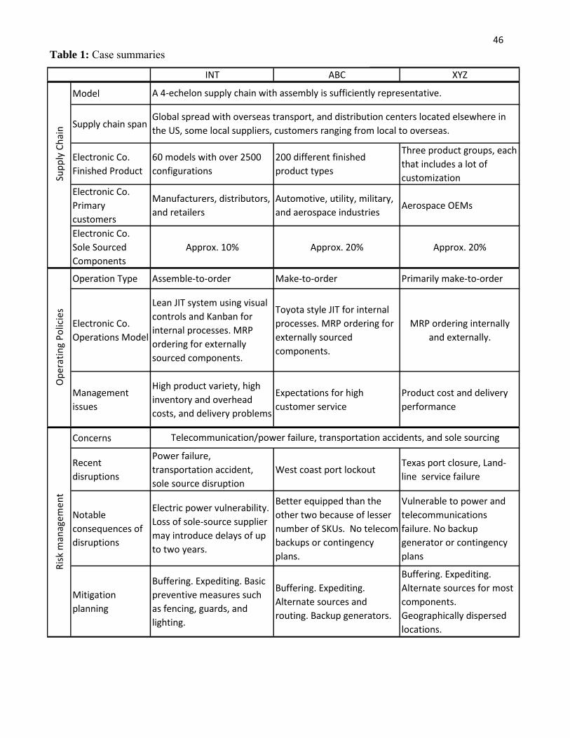
46
INT ABC XYZ
Model
Supply chain span
Electronic Co. Finished Product
60 models with over 2500 configurations
200 different finished product types
Three product groups, each that includes a lot of customization
Electronic Co. Primary customers
Manufacturers, distributors, and retailers
Automotive, utility, military, and aerospace industries
Aerospace OEMs
Electronic Co. Sole Sourced Components
Approx. 10% Approx. 20% Approx. 20%
Operation Type Assemble‐to‐order Make‐to‐order Primarily make‐to‐order
Electronic Co. Operations Model
Lean JIT system using visual controls and Kanban for internal processes. MRP ordering for externally sourced components.
Toyota style JIT for internal processes. MRP ordering for externally sourced components.
MRP ordering internally and externally.
Management issues
High product variety, high inventory and overhead costs, and delivery problems
Expectations for high customer service
Product cost and delivery performance
Concerns
Recent disruptions
Power failure, transportation accident, sole source disruption
West coast port lockoutTexas port closure, Land‐line service failure
Notable consequences of disruptions
Electric power vulnerability. Loss of sole‐source supplier may introduce delays of up to two years.
Better equipped than the other two because of lesser number of SKUs. No telecom backups or contingency plans.
Vulnerable to power and telecommunications failure. No backup generator or contingency plans
Mitigation planning
Buffering. Expediting. Basic preventive measures such as fencing, guards, and lighting.
Buffering. Expediting. Alternate sources and routing. Backup generators.
Buffering. Expediting. Alternate sources for most components. Geographically dispersed locations.
Telecommunication/power failure, transportation accidents, and sole sourcing
Risk m
anagem
ent
Ope
ratin
g Po
licies
Global spread with overseas transport, and distribution centers located elsewhere in the US, some local suppliers, customers ranging from local to overseas.
A 4‐echelon supply chain with assembly is sufficiently representative.
Supp
ly Cha
in
Table 1: Case summaries
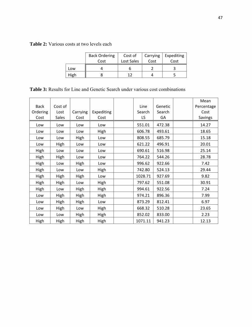
47
Table 2: Various costs at two levels each
Back Ordering
Cost Cost of
Lost Sales Carrying Cost
Expediting Cost
Low 4 6 2 3 High 8 12 4 5
Table 3: Results for Line and Genetic Search under various cost combinations
Back Ordering Cost
Cost of Lost Sales
Carrying Cost
Expediting Cost
Line Search LS
Genetic Search GA
Mean Percentage
Cost Savings
Low Low Low Low 551.01 472.38 14.27 Low Low Low High 606.78 493.61 18.65 Low Low High Low 808.55 685.79 15.18 Low High Low Low 621.22 496.91 20.01 High Low Low Low 690.61 516.98 25.14 High High Low Low 764.22 544.26 28.78 High Low High Low 996.62 922.66 7.42 High Low Low High 742.80 524.13 29.44 High High High Low 1028.71 927.69 9.82 High High Low High 797.62 551.08 30.91 High Low High High 994.61 922.56 7.24 Low High High High 974.21 896.36 7.99 Low High High Low 873.29 812.41 6.97 Low High Low High 668.32 510.28 23.65 Low Low High High 852.02 833.00 2.23 High High High High 1071.11 941.23 12.13
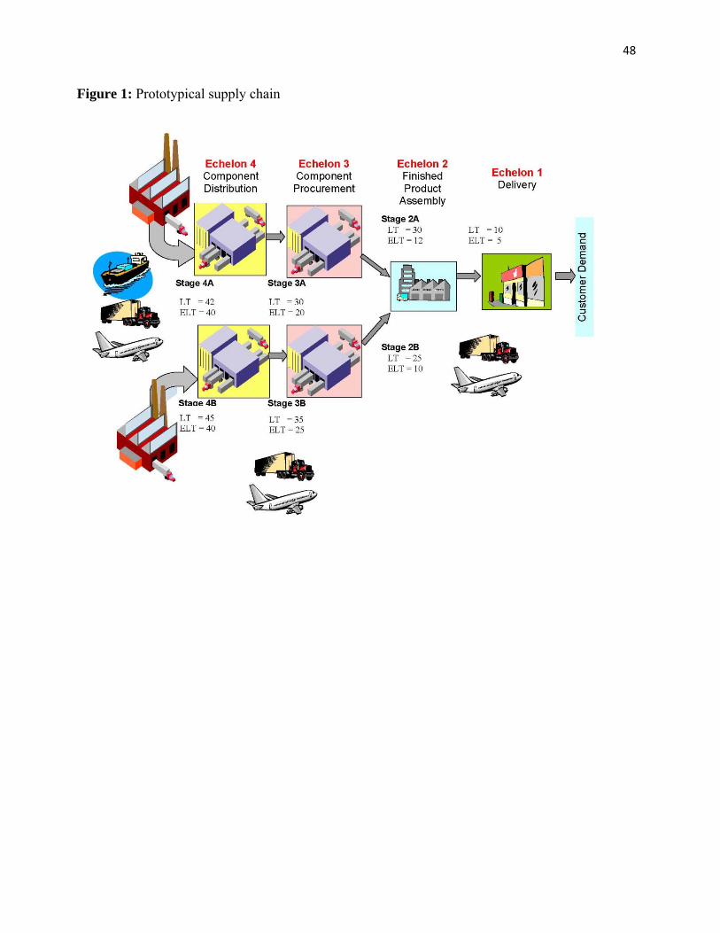
48
Figure 1: Prototypical supply chain
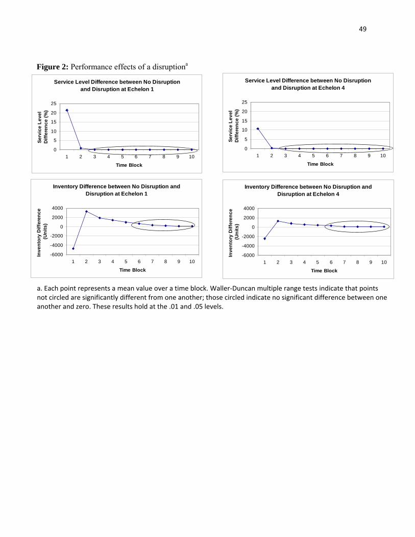
49
a. Each point represents a mean value over a time block. Waller‐Duncan multiple range tests indicate that points not circled are significantly different from one another; those circled indicate no significant difference between one another and zero. These results hold at the .01 and .05 levels.
Figure 2: Performance effects of a disruptiona
Service Level Difference between No Disruption and Disruption at Echelon 1
0
5
10
15
20
25
1 2 3 4 5 6 7 8 9 10
Time Block
Serv
ice
Leve
l D
iffer
ence
(%)
Inventory Difference between No Disruption and Disruption at Echelon 1
-6000
-4000
-2000
0
2000
4000
1 2 3 4 5 6 7 8 9 10
Time Block
Inve
ntor
y D
iffer
ence
(U
nits
)
Service Level Difference between No Disruption and Disruption at Echelon 4
0
5
10
15
20
25
1 2 3 4 5 6 7 8 9 10
Time Block
Serv
ice
Leve
l D
iffer
ence
(%)
Inventory Difference between No Disruption and Disruption at Echelon 4
-6000
-4000
-2000
0
2000
4000
1 2 3 4 5 6 7 8 9 10
Time Block
Inve
ntor
y D
iffer
ence
(U
nits
)
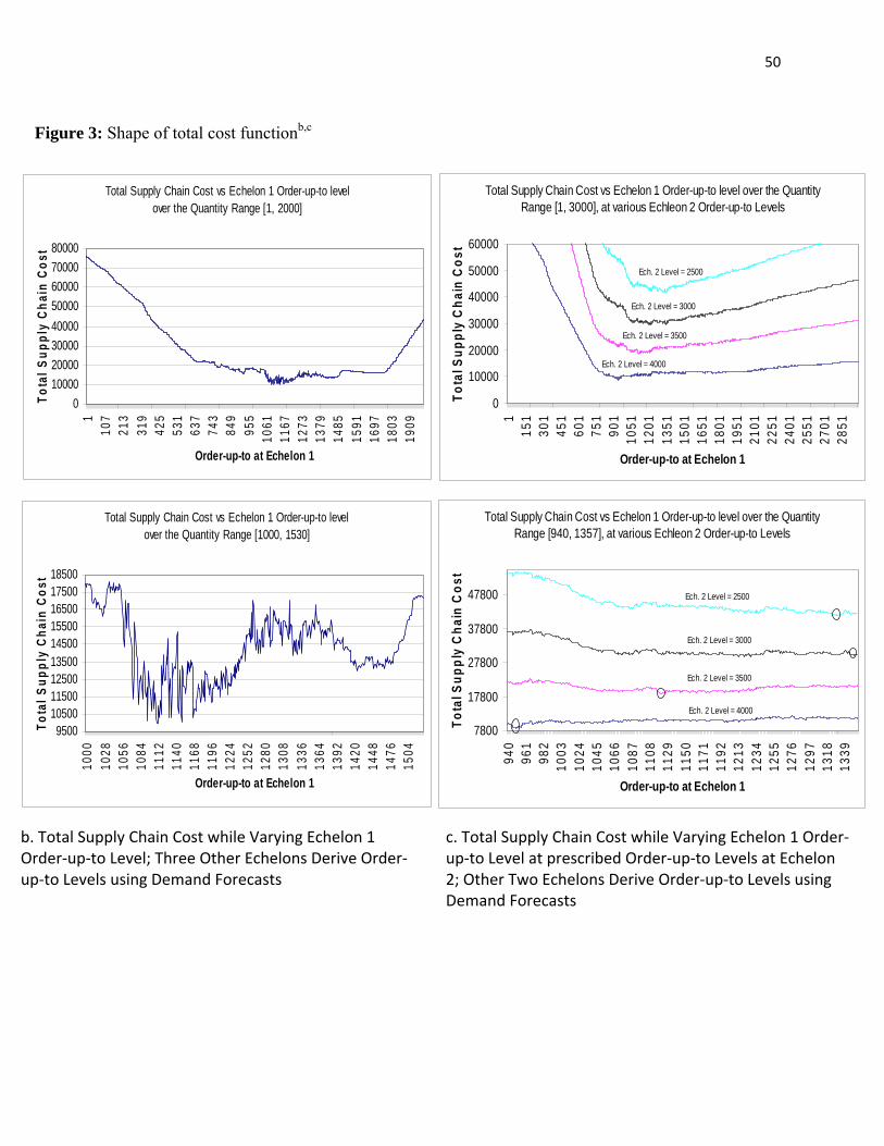
50
b. Total Supply Chain Cost while Varying Echelon 1 Order‐up‐to Level; Three Other Echelons Derive Order‐up‐to Levels using Demand Forecasts
c. Total Supply Chain Cost while Varying Echelon 1 Order‐up‐to Level at prescribed Order‐up‐to Levels at Echelon 2; Other Two Echelons Derive Order‐up‐to Levels using Demand Forecasts
Total Supply Chain Cost vs Echelon 1 Order-up-to level over the Quantity Range [1, 2000]
01000020000300004000050000600007000080000
110
721
331
942
553
163
774
384
995
510
6111
6712
7313
7914
8515
9116
9718
0319
09
Order-up-to at Echelon 1
Tota
l Sup
ply
Chai
n C
ost
Total Supply Chain Cost vs Echelon 1 Order-up-to levelover the Quantity Range [1000, 1530]
9500105001150012500135001450015500165001750018500
1000
1028
1056
1084
1112
1140
1168
1196
1224
1252
1280
1308
1336
1364
1392
1420
1448
1476
1504
Order-up-to at Echelon 1
Tota
l Sup
ply
Cha
in C
ost
Figure 3: Shape of total cost functionb,c
Total Supply Chain Cost vs Echelon 1 Order-up-to level over the Quantity Range [1, 3000], at various Echleon 2 Order-up-to Levels
0
10000
20000
30000
40000
50000
60000
115
130
145
160
175
190
110
5112
0113
5115
0116
5118
0119
5121
0122
5124
0125
5127
0128
51
Order-up-to at Echelon 1To
tal S
uppl
y C
hain
Cos
t
Total Supply Chain Cost vs Echelon 1 Order-up-to level over the Quantity Range [940, 1357], at various Echleon 2 Order-up-to Levels
7800
17800
27800
37800
47800
940
961
982
1003
1024
1045
1066
1087
1108
1129
1150
1171
1192
1213
1234
1255
1276
1297
1318
1339
Order-up-to at Echelon 1
Tota
l Sup
ply
Cha
in C
ost
Ech. 2 Level = 2500
Ech. 2 Level = 3000
Ech. 2 Level = 3500
Ech. 2 Level = 4000
Ech. 2 Level = 2500
Ech. 2 Level = 3000
Ech. 2 Level = 3500
Ech. 2 Level = 4000
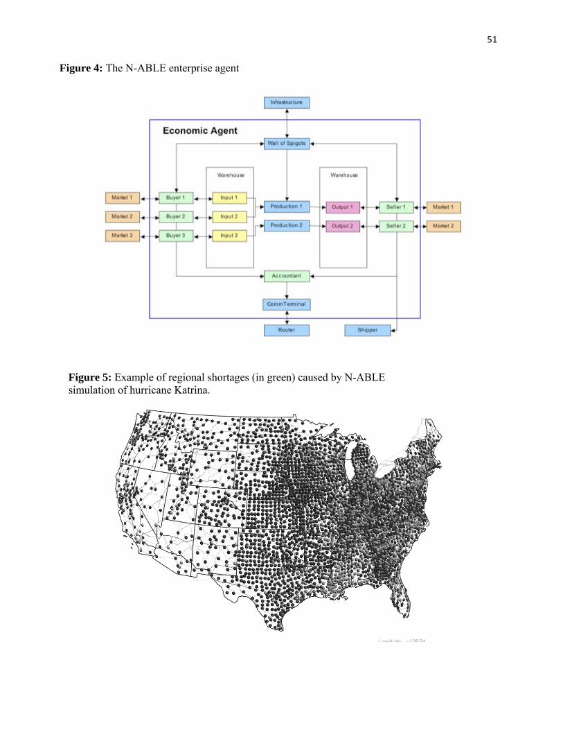
51
Figure 4: The N-ABLE enterprise agent
Figure 5: Example of regional shortages (in green) caused by N-ABLE simulation of hurricane Katrina.