Hitotsubashi University Repository

Title Modeling Dualistic Development in Japan

Author(s) Minami, Ryoshin; Ono, Akira

Citation Hitotsubashi Journal of Economics, 18(2): 18-32

Issue Date 1978-02

Type Departmental Bulletin Paper

Text Version publisher

URL http://doi.org/10.15057/7971

Right

MODELlNG DUALISTIC DEVELOPMENT IN JAPAN

By RYOSHlN MlNAMI AND AKIRA ONO*

I. Introductron

(1) Purpose of This Study One of the most distinguished characteristics of the prewar Japanese economy is, in

the writers' opinion, the dual structure or the co-existence of the subsistence and capitalist

sectors. That is to say agriculture and small scale establishments in non-agriculture belong

to the former sector characterized by surplus labor or unlimited supplies of labor (USL),

while other industries, mostly based on modern technology, comprise the latter sector

characterized by the marginal principle. Such an understanding of the Japanese economy,

which is usually referred to as the "classical approach," is in contrast with the "neo-classical

approach," which assumes the marginal principle for all industries. (The dual structure

in this sense is not and cannot be treated in the latter approach.) Japan has been a bat-

tlefield of the controversy between the two approaches. The former approach has been

claimed by Lewis, Fei-Ranis, Ohkawa, Minami and others, while the latter approach has

been taken by Jorgenson, Keuey-Williamson, and others.1 There is no need in this paper,

however, to argue the applicability (inapplicability) of the classical (neo-classical) approach,

because full scale arguments have been made by Minami in his book in 1973.2

Relying on his conclusion in that book, that the classical approach was applicable until

around 1960, a model with an emphasis on the labor market will be set forth following this

approach and estimated using Japanese statistics in Section II. Based on this model some

simulation tests will be attempted in Section 111. They will shed light on the mechanism

and the features of economic growth in prewar Japan. Such a simultaneous equation ap-

proach must be much more efficient than ordinary approaches of "comparative statics" and "comparative dynamics," because of simultaneous relations among economic variables.

The model estimated in this paper can be taken as an econometric version of the theory of

economic developemnt ~ la Lewis and Fei-Ranis.3 Simulation study in Section 111 will

~ Professors (Kyo~'ju) of Hitotsubashi University and Seikei University, both in Tokyo, Japan. The writers

are indebted very much to Professors Kazushi Onkawa. Hugh T. Patrick and Gustav Ranis for their encour-agement and useful comments on the original version of this paper. Much thanks are also due to Mr. Edward Lincoln for his editing the English. This study was partly undertaken as a component of the Population and

Employment Project, world Employment Programme, International Labour Organisation. * See Lewis [1958], Fei and Ranis [1964], Onkawa E1972]. Minami [1968] [1973]. Jorgenson [1966], and

Kelley and Wilnamson [1974]. Among the economists who claim the classical approach, there is a difference in demarcating the turning point; it is 191(~19 for Fei-Ranis and around 1960 for Ohkawa and Minami.

' The assertion of the tuming point occurring in about 1960 (Minami [1968] [1973]) seems to be favorably accepted in and out of the academic cirde in Japan partly because it is consistent with the ~idely hdd view that her economy shifted trom a tabor surplus to a labor shortage phase at that time.

' Lewis [1954]. Fei and Ranis [1964].

MODELING DUALISTIC DEVELOPMENT lN JAPAN 19 give a test of applicability of some conclusions, attained by Lewis and Fei-Ranis in their

theoretical studies, in light of the Japanese experiences. Major findings and their implica-

tions will be sumJnarized in Section IV. Coming to the study in Sections 11 and 111, it may

be pertinent to give a survey of the sectoral changes in wages and employment in the last

part of this section.4

(2) Overview of Sectoral Wages and Employment Let us study the changes in wages and employment by three industry groups; A (primary),

M (mining, manufacturing, construction and facilitating) and S (other industries, mainly

services and commerce, including government). Wages defiated by the consumer price index (P!.) given in Panel A of Table I demonstrate different pattern of changes among

sectors :5 The exponential rate of growth6 for the entire period (1906-40) is the highest

in M (2.53 percent per annum) and the lowest in A (0.37 percent).7 S Iies between them

(1.25 percent). This difference in the rate of growth comes mainly from the fact that wages

continued to rise steadily in M, while decreasing in A and, to a lesser extent, in S, for the

years since the middle 1920's.

During the downswing in the 1920's big enterprises used some devices to mitigate the

TABLE I . REAL WAGES BY THREE INDUSTRY GRoUP, WAGE DIFFERENTIALS AMoNG THREE INDUSTRY GRoups, AND PERCENTAGE OF SURPLUS LABOR IN SECTOR I LABOR FORCE

A

M S

M/A JV[/S

L*/L 1

1906-10 1911 15 1916~20 1921 '5 1926-30 1931 35 193~40

A.

0.78 (0.94)

0.83

0.64

B.

l . 06

1 . 30

C.

59.9

Real Wages (Yen)

0.82 0.95 l.lO

(0.96) (1 .29) (1 .47) 0.85 O.99 1 .39

0.66 0.82 1.13

Wage Differentials

l .04 1 . 04 1.26

1 . 29 l.20 l . 23

Percentage of Surplus Labor in Sector

53.2 54.9 68.7

1.08 (1.36)

l.53

l .09

0.79 (0.84)

1.60

0.89

0.901 (O. 9 1 l)

- .461

0.8 1 1

l .42 2.03 1 . 621

l .40 l.80 l . 80*

1 (A+S) Labor Force (~)

66.3 53.7 43.8

Remarks: Means for respective five years. (Istands for 1 936-39.) Real wages stand for daily wages for production workers deflated by consumer price index (P/.). Figures in parentheses are wages deflated by the rural consumer price index (P!.).

Sources: For wage statistics see Minami and Ono [1978]. P/ is from Ono and Watanabe [1976]. For L and L* see Statistical Appendix and Section 11 (1) respectively.

' There are two reasons why this study starts from 1906. The first is that statistics on labor and capital by industry group are available from this year. The second is that equilibrium theory does not seem to be ap-plicable during the early phase of modern economic growth, in which the national markets on labor, capital

and output did not exist in their full shapes. See Ono and Watanabe [19761 and Ueno and Teranishi [19751, pp. 371-373.

5 For detailed discussions of the changes in sectoral wages, see Minami [1973], Chs. 7 and 8 and Minami and Ono [1978],

e The exponential rate of growth for the variable 'X' is estimated as the parameter 'b' in the regression

equation ln Xt =a+bt. T Wages for A deflated by the rural consumer price index (P!.), which are shown in Panel A, do not show

any increasing trend at all. The annual exponential rate of growth for 1906-39 is -0.14 percent.

HITOTSUBASHI JOURNAL OF ECONoMlcs

decline in profits. These were comprised of mechanization of production processes depend-

ing on borrowed technology and rationalization of labor management. Referring to the

latter, these enterprises reduced the demand for unskilled labor and kept skilled workers

in their own firms. As a device for keeping skilled workers, the lifetime employment system

peculiar to Japan, appeared in this particular period. Consequently, while unskilled workers

became redundant or unlimited in supply, skilled workers continued to be limited. A different pattern of changes in sectoral wages give rise to changes in wage differentials among

sectors. According to Panel B, the wage ratios of M to A and to S increased in the 1920's

and the first half of the 1930's. This leads us to such important inferences as follows : 1)

The Japanese labor market was characterized by a co-existence of separated markets for

unskilled and skilled workers. 2) Almost all the labor force in A and a large protion of the

labor force in S was comprised of unskilled workers, whereas in Sector M skilled workers

were dominant. Along with the course of economic development the industrial composition of employ-

ment suffered from big changes; employment as a percentage of total employment increased

both in Sectors M and S, respectively from 18.4 percent (1909) to 27.9 percent (1937) and

from 20.8 percent to 26.8 percent, whereas it decreased in Sector A from 60.8 percent to

45.3 percent. (All figures are based on seven year averages.) A much more interesting finding is about the pattern of changes in the growth rate of sectoral employment. In Fig.

FIG. 1. GROWTH RATES OF LABOR FORCE BY THREE INDUSTRY GROUP

(~) 5

4

3

2

l

o

-1

lr'l ,, A 1,

'L.

G (L*)

r4( ,)l

-1 A t fJ' l' t/ tJ. V "t

l ¥ ¥

/ ~ j

'L

JPd

f l I I l , ~

,~

f t

A / ¥ff~lL

G (Ls)

G (L.)

G (L4 + Ls)

~, L1

L. (%)

lr¥ ¥t ¥1 ¥ L

3

2

1

o

-1

Remarks:

1905 lO 15 20

G(X)=100 (X-X_1)/X_1'

25 30 35 40 ~ ear

Figures for 'X' are seven year moving averages.

21 1978] MODELINC DUALISTIC DEVELOPMENT IN JAPAN

1 the growth rate for Sector M employment (LM) increased sharply during the upswings

before 1919 and after 1931, whereas it decreased remarkably during the downswing between

these two years. On the other hand both the growth rate of Sector A employment (LA) and

that of Sector S employment (Ls) and therefore LA +LS tended to fluctuate in opposite direc-

tions from the long swings.8 These findings are compatible with our assumption that LM

tended to be determined by the demand for labor in Sector M and on the other hand LA+Ls

was determined as a residual.

II. Modeling

(1) Labor Market It may not be far from reality to assume that the Sector I (Sectors A and S) workers

are all unskilled, whereas the Sector 2 (Sector M) workers are composed of two groups

unskilled and skilled workers, and that unskilled workers in Sector I are supplied unlimitedly

TABLE 2. LIST OF NoTATIONS

,

Subscript (j)

V=_ylV,. Vt=Vjl/Pj!

Vj!

I=~]ls' Is I h

lg~

lg=~Igj, Igj

B S=1+1h+1g~+1g+B Wj = W f IPj!

Wjl P = P1//P2!

p jl

p./

L=~}LJ, Lj

L*

N Z Q K=~)Kj, KJ A hj u

~J

t

1 =subsistence sector

2=capitalist sector

GDP at constant (1934-36) prices

GDP at current prices (million yen)

private fixed investment at constant pr]ces (million yen)

housing investment at constant prices (million yen)

military expenditure at constant prices (million yen)

government fixed investment at constant prices (million yen)

surplus on current account at constant prices (million yen)

gross saving at constant prices (million yen)

real wages

money wages (yen)

relative price index (1931~36=1)

output price indexes (1934~36=1)

consumer price index (1931~36=1)

the number of employees (million persons)

surplus labor in Sector I (million persons)

total population (million persons)

rate of school attendance

rate of working age population

gross capital stock at constant prices (million yen)

area of cultivated land (thousand hectares)

labor hours per year (1934-36=1)

utilization rate of capital asset in Sector 2

utilization rate of land

rate of discard of capital stock

year (1 ....35 for 1906....40)

8 Changes in Sector A employment and its determinants have been fully studied in Minami [1973]. Ch. 6.

22 ruTOTSUBASHI JOURNAL OF EcoNoMJcs [February , to Sector 2,9 while the supply of skilled workers in Sector 2 is limited.ro With these assump-

tions one may see that we can explain the emergence of wage differentials. An important

corollary of these assumptions is that employment in Sector 2 is determined first so that

maximum profits are attained and the rest of the workers are absorbed in Sector I , a pool

of surplus labor.n

According to these assumptions Sector I wages in terms of its sector products (Wl= W1!jP1/), as a substitute for wages deflated by P./, are exogenously given.12 On the other

hand, Sector 2 wages in terms of its sector products (W2= W2//P2/) are a wei_~hted average

of the wages for unskilled and skilled workers. Unskilled worker wages tend to change according to the supply price of labor or Sector I wages. Skilled worker wages are deter-

mined by their marginal revenue product because of the assumption of limited supplies of

labor. Therefore W2 can be basically expressed as a function of Sector I wages in terms

of Sector 2 products (PW1=W1//P2/) and the average labor productivity in Sector 2 (V2/L2), which is a proxy variable for the marginal revenue products of skilled workers.13

In addition to these basic variables, time trend (t) is included in equation (1) to express a

change in the composition of workers by skill. A negative parameter for this variable may

imply an increasing weight of unskilled workers. (See Table 3.) The parameter of W2, _1

signifies that Sector 2 wages tend to follow the supply price of labor of the Sector I workers

and the labor productivity in Sector 2 with a lag of about six months. In Sector 2 the

g As one of the major evidences for the existence of unlimited supply of labor (USL), Minami pointed out the fact that real agricultural wages were much higher than marginal labor productivity ([1973], pp. 205-206).

The same conclusion has been obtained in the present study; i.e., the output elasticity of labor in Sector I is

estimated to be 0.350 (equation (4) in Table 3), whereas the relative income share of labor in this sector is 0.604. O.704 and 0.568 on the average for 1906-20, 192i-30 and 1931-40 respectively.

lo Note that the hypothesis of unlimited supplies of labor formulated by Lewis refers to unskilled labor, whereas limited supplies of skilled labor are also assumed by Lewis ([1954], p. 406 [reprinted version]).

ll urplus labor or disguised unemployment, which is denoted by L*. is defined here as the labor force for which marginal productivity is much smaller than wages (W1)'

12 An explanation for determination of the "subsistence leve] " or the "institutional wages" (Wl!/Pl!) js

not attempted in this study. This level is considered to be dependent upon various factors. economic as well as non-economic. A wide-range study covering economics as well as the other social scuences is needed in this respect. The substitution of Wl!/Pl/ for Wl!/P./ js found in a formulation of the Lewisian theory by

Fei-Ranis [1964]. By means of this assumption we can drop one variable (P.!/P2/) and the equation wh[ch explains this variable in the econometric model developed below.

13 The significance of this formulation is that the wage differential between the sectors tends to emerge with an increase in labor productivity in Sector 2. If statistics for wages and the size of the labor force for

both skilled and unskilled workers in Sector 2 were available, a wage determination function could be estimated

for each of the two types of workers.

14 The equilibrium condition in Sector 2 is written as 1 1 V2 ¥* ( ) = - (x L~. ' W The left hand side of the equa p

tion represents an equilibrium value of the marginal revenue product of labor, where a is the elasticity of demand for output with respect to price, and p is the output elasncity with respect to labor. There elasticltles

are assumed to be constant through time. We have such a partial adjustment model as

V2 {(~~) _(J~) }, V2 V* V

( - )( = )

A L2 L~2 L

_ where I is a fraction of the difference between the desired and actual levels in V2/L2' Combining the above two equations, we have

V2_ A V~ ( -l )

W2+(1 -1) L~2~ L~~'s (1 1 ) -

i a

By estimating this equation and using an estimate for P in the production function (equation (5) in Table 3),

we can calculate a and 1.

19781MODELING　DUALETIC　DEVELOPMENT　IN　JAPAN 23

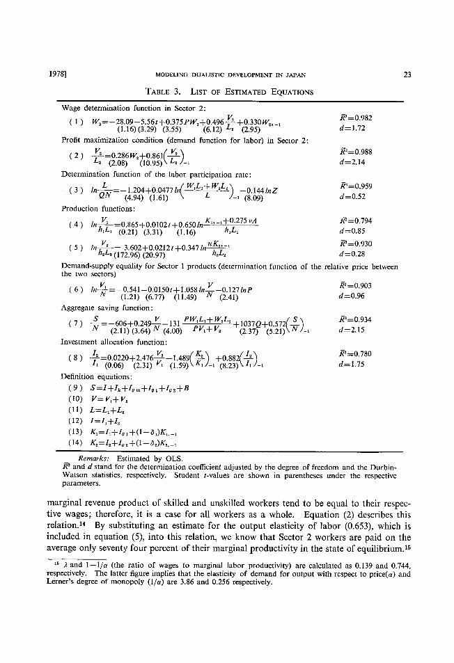
TABLE3．　LlsT　oF　EsTIMATED　EQuATloNs

Wage　determination　function　in　S㏄tor2：

　　　　　　　　　　　　　　　　　　　　　　　　　　　　　　　レ㌔　　　　　　　　　　　　　　　　　　　　　　　　R2＝0．982　（1）　　昭2＝一28．09－556∫十〇．375、PレV1十〇，496　　　十〇．330鴎，＿1　　　　　　　　　　（1．1㊦（3．29）（3．55）　（6，12）L2（2，95）　　　　　4ニ1・72

Pro飢maximization　condition（demand　function　for　labor）in　S㏄tor2：

（2）髪マ9：辮8：離）、、　　　　嵩188Detemination　f㎜ction　of　the　labor　participation　rate：

（3）’η赤一（互：lll欄71n（曜1LI圭鴎L2）一、謂加Z　　灘59

Production　functions：

（4）Z誤＿0．865＋0．OIO2，＋0．6501πκ【・一1＋0・275vイ　　　　R2ニ0・794　　　　　　　h1L・（0，21）（3，31）（1．16）　海ΣL・　　　　　　ゴー0。85

（5）1’～ろ＿3．6・2＋・．0212∫＋。．347Zn麗κ2・一1　　　　　　π2－0・930　　　　　　　h2L2（172．96）（20．97）　　　h2L2　　　　　　　ゴニ028

Demand－supply　equality　for　Sector　l　products（determination　function　of　the　rela亡ive　price　between

thetwosectors）

（6）1’年聡＿0．541＿0．0150ご＋1．0581nヱ＿0．127，πP　　　　　π2－0・903　　　　　　　ノ〉　（1．21）（6．77）（11．49）押（2．41）　　　　　　4＝0．96

Aggregate　saving　function：

（・）亮一翻：離（、1δ1）P写讐2＋齢2：ll縄）．、魏34

1nvestment　al1㏄ation　function：

（8）会π8：8言1・キ1：窒絢：鍔（暑）『、瀞会）一、　　黎80

Definition　equations：

　（9）S＝1＋1ん＋1佛＋1σ、＋192＋B

　（10）　V＝V1十V2

　（11）　L＝＝L1十L2

　（12）　1＝11十」颪2

　（13）・κ1＝1、＋19、＋（1一δ、）K、，一、

　（14）κ2＝12＋192＋（1一δ2）κ2，一、

　　　、Rθ耀αたs』　Estimated　by　OLS，

R2and4stand　for　the　determination　coefficient　adjusted　by　the　degree　of　freedom　and　the　Durbin－

Watson　statistics，respectively．Student’一values　are　shown　in　parentheses　under　the　respective

parameters，

marginal　revenue　product　of　skilled　and　unskilled　workers　tend　to　be　equal　to　their　respec－

tive　wagesl　therefore，it　is　a　case　for　all　workers　as　a　whole．　Equation（2）describes　this

relation。14　By　substituting　an　estimate　for　the　output　elasticity　of　labor（0．653），which　is

included　in　equation（5），into　this　relation，we　know　that　Sector2workers　are　paid　on　the

average　only　seventy　four　percent　oftheir　marginal　pro（1uctivity　in　the　state　ofequilibrium．15

　15λand1－1／α（the　ratio　of　wages　to　marginal　labor　productivity）are　calculated　as　O．139and　O，744，

resp㏄tively。The　latter五gure　implies　that　the　elasticity　of　demand　for　output　with　respect　to　price（α）and

Lemer’s　degr㏄of　monopoly（1／α）are3．86and　o．256respectively．

24 HITOTSUBASHI JOURNAL OF ECONOMICS [February

Combining equations (1) and (2), W2 and V2/L2 are determined. From the value for V2iL2 and the production function in Sector 2, the labor force in this sector (L2) is known.

The employment in Sector I (L1) is determined as L1=L-L2 (equation (11)). L1 is com-posed of the surplus labor (L*) and the labor force whose marginal productivity (MPL1) is

not smaller than the real wages (W1)' The size of the latter labor force can be calculated

from the relation Wl=MPL1, where MPLI is known from the production function (4). The ratio of L* to L1' which is shown in Panel C of Table 1, shows a negative relation to

long swings. This relation comes from the negative association between L1 and long swings

that are studied in Section I (2). Total labor supply (L) is given by the size of working age

population (QN), which is given exogenously,16 and the labor participation rate (L/QN).

The latter comes from equation (3), which relates L/QN positively with the average wages

( ( WIL1+W2L2 ~ ~ and negatively with the rate of

in the economy in the previous year ~ L )_1)

school attendance (Z).

(2) Other Markets Output Market: Outputs of both sectors (VI and V2) are determined by the produc-

tion functions (4) and (5) respectively. Multi-co]inearity among variables makes it dif-

ficult to estimate these functions. This is the reason why an arbitrary assumption was made

in estimating each of them. That is, two kinds of assets, capital and land, are aggregated

into one variable in (4)17 and the output elasticity of capital was taken from a cross-sectional

study of manufacturing in (5).rs One of the interesting findings here is a gap in the rate

of growth in total factor productivity between the two sectors; 1.02 percent and 2.1 1 percent

in Sectors I and 2 respective]y. This gap explains 44.5 percent of the difference in the rate

of growih in labor productivity. Products of the two sectors are put on the market, where

the relative price (P) changes flexibly so that the market is cleared.19 That is to say, we

assume that supply and demand tend to be equal to each other with respect to both of the

two sector products. Owing to Walras' Law, however, one can drop one of the equilibrium

conditions for the two output markets; here the market for Sector 2 products is eliminated.

From the demand function for Sector I products and the equality of supply and demand,

we have equation (6) which relates VliN with V/N, P and t.20 Time trend is included to explain exogenous factors affecting the demand for Sector I products; i.e., changes in the

** We assume that N and Q are exogenously given. This is because we consider that the assumption is rather realistic in the observation period and consistent with the theories of Lewis and Fei-Ranis : Lewis adrnitted the possibility of a decline in the death rate and consequently a rise in the natural rate of increase

with rising per capita income ([1954] pp. 404~05 [reprint version]); however. such a notion is not integrated

into his theory of economic development. In the model by Fei-Ranis, population is explicitly treated as an

exogenous variable ([19641, p. 228). *' The constant (0.275) attached to the variable A in the production function of Sector I stands for the value

of land assets per thousand hectare at 1934-36 million yen (LTES, Vol. 9, p. 221). 18 Means of the annual cross-sectional estimates by Shinohara ([1949], p. 209) for the output elasticities of

capital and labor in manufacturing for 1929-40 are 0.3321 and 0.6239 respectively. Dividing these figures by their sum (0.9560) one may obtain the elasticities under the assumption of constant returns to scale.

" A theoretical basis for this formulation of relative price determination is found in Fei-Ranis [1964], pp.

155-159. This formulation is believed to hold in the prewar Japanese economy. 'Q The demand function for Sector I products is expressed as Xd=F*(V/N, P, t), where the first derivatives

for V/N and P are positive and negative respectively. In equilibrium we have Xd=X"=X, where X~ and X stand for the supply of and the actual quantity (domestic production+import-export) of the Sector I prod-ucts. Substituting V* for X, we have V*=F*(V/N, P, t). An implicit assumption in this formulation is that

consumption behavior is the same between the labor force components in the two sectors.

1978] MODELING DUALISTIC DEVELOPMENT IN JAPAN 25

taste of consumers, foreign trade and so forth. V1 and V2 being given by production functions, P is determined through this equation. An implication of this equation is that

P tends to increase along with the process of industrialization or a rise in V2 as a percentage

of V.

Capita/ Market.' Gross saving (S) is determined through a saving function (7). The

long-term marginal propensity to save is calculated as 0.582, which seems to be too large;

inclusion of government saving in S may be responsible for this result.21 The negative parameter for the relative income share of labor in the economy as a whole (PWILl+ W2L2)/

(pVl+ V2) signifies that the increasing trend and fluctuations related to long swings in S/N

were partly attributable to a decreasing trend and fluctuations negatively associated with

long swings in the relative share respectively. These associations between savings and

the relative income share, which come from the fact that the propensity to save is much

lower in wage income than in non-wage income,22 are very important in that through these

associations income distribution tends to affect the rate of capital accumulation and the

rate ofeconomic growth. The parameter for the ratio of working age population (Q) implies

that the propensity to save is higher accordingly as the share of working age population is

larger.

Substituting S into relation (9), the saving-investment identity, private fixed investment

(1) is obtained, as housing investment (Ih), military expenditure (Ig~), government fixed

investment (Ig* and lg,) and net exports (B) are given from outside of the model. I is allo-

cated into the two sectors based on equation (8). Considermg the "caprtal stock adJust ment principle" in investment behavior, the output ratio (V2/Vl) and the capital stock ratio

in the previous year ((K2/K1)-1) are taken to explain 12/11'23 Another five equations are

needed to complete the model. Equations (10), (11) and (12) give the definitions of V, L

TABLE 4. RESULTS OF THE FlNAL TEST-THEIL'S INEQUALITY COEFFICIENT

Vl V2

K*

K2

Ll

L2 I1 I!

S W2 P

0.086

0.1 13

0.136

0.l06

0.064

0.210

0.425

0.399

O.277

0.071

O.387

2* specially, a rapid increase in I. during the years of military expansion seemed to give an upward bias to the estimate of the propensity to save. Estimating the saving function by using S-1g~ in a place of S, the marginal propensity to save in a long-run equilibrium state decreases to 0.337.

2, In his theory Lawis assumes that all savings are done by people who receive profits or rents ([1954], p. 417

[reprint version]). Our saving function is a general formulation of his view. If savings data were available for different income groups we could estimate different savings functions for the respective groups. Also it should be interesting to estimate these functions by sector, if savings data by sector were available.

" nfortunately there are no explicit arguments on the investment allocation in the theories by Lewis and Fei-Ranis, in which it is simply assumed that all savings are invested in the capitalist sector. This assump-

tion is not realistic.

26 HITOTSUBASHI JOURNAL OF ECoNoMlcs [February and I respectively. Equations ( 1 3) and (14) show the relation between investment and capital

stock. Comparison between generated and actual figures for respective endogenous varia-

bles will help us evaluate a fitness of this model to the economy. (See Table 4.) Except for

Il' 12, P and S, fitness of the model is pretty good.

III. Simulation Analysis

Now we are in a position to make simulation tests based on the model estimated above.

By comparing the values which are estimated under several assumptions with the values in

the final test, one may argue about the effects of these assumptions on the growth and

structure of the economy. Table 5 gives ratios of the former values (simulation test) to the

latter values (final test) for endogenous variables and some combinations of them for the

last decade (1931-40), this ratio being called the S-F ratio in short. Because the former is

equal to the latter in the initial year, the S-F ratio larger (smailer) than unity signifies that

the variable in question increases much faster (more slowly) in the hypothetical case than

what it actually did.

(1) Population and Labor Supply In Test A the total population (N) is assumed to be constant at the 1906 Ievel in place

of the actual increasing trend.24 Two major findings are noted here. l) The rate of growth

in GDP (V) is much lower with slower population growth. This comes from the fact that a negative effect of a slower increase in labor supply tends to offset a positive effect of the

slower increase of population which stimulates savings (by decreasing basic consumption)

and capital accumulation. V/N and W2 tend to increase with the slower increase ofpopula-

tion. 2) Sector I employment (Ll) decreases because of a larger decrease in labor supply_

(L) than a decrease in the demand for labor in Sector 2 (L2)' Owing to a decrease in Ll' Iabor

productivity in Sector I (V1/L1) increases, Ieading to decreases in the size and the propor-

tion of surplus labor (L* and L*/L1)' Surplus labor in expected to disappear or the turning

point is passed in 1940 in this hypothetical case.25

Implications of these findings are as follows :26 the first finding implies that if the rate

of population increase had been much higher in Japan, the rates of growth in GDP and per

capita GDP would have been, respectively, higher and lower than what they actually were.

The fact that the rate of economic growth in Japan was higher than in any other countries,

whereas her rate of population increase was not high in international comparison,27 seems

to show at a glance a non-existence of the relationship between economic growih and popula-

tion increase. This view has been revealed to be superficial. The second finding seems to

" The annual exponential rate of growth of N is I .29 percent. 2* After the turning point is passed, W* is no longer exogenous. It is expected to increase in parallel fashion

with the marginal productivity of labor in Sector I . What actually happened after the turning point about 1960 was a rapid increase in real wages for unskilled workers and narrowing wage differentials (see Minami [1973L Chs. 7 and 8).

~6 In addition to Test A, which provides the case with zero population growth, we have attempted some simulation tests for hypothetical cases of population increase at alternative rates of growth (1 and 2 percent

per annum) and obtained just the opposite conclusions to those in Test A. That is to say, the model is con-sistent in that endogenous variables move in the opposite direction. This is the case for all simulation tests

below.

27 Kuznets [1971], Tables I and 3.

1978] MODELING DUALISTIC DEVELOPMENT IN JAPAN 27

support the commonly held view that an increase of surplus labor can partly be attributed

to rapid population growth and implies that the turning point could have been reached earlier

if the rate of population increase had been lower. In light of the conclusion a decline in the

rate of population increase in the post World War 11 period may be identified as one of the

factors for passing the turning point in about 1960.28

An implicit assumption of the discussion above is that a change in the rate of popula-

tion growth does not alter the age composition of population. However a decrease in the

rate of population growth based on a decrease in the birth rate is usually followed by aging

of the population, which is simply expressed in our model by a rise in Q. Effects of a rise

in Q are clarified by Test B, in which Q is assumed constant at the 1906 Ievel in place of its

TABLE 5. MEANs OF THE RATIOS OF SIMULATION TESTS To FINAL TEST FOR 1931-40 (S-F RATros)

v* v, v K* K2

K L* L, L

v,/L*

vz/L2

V/L V/N

I* 12 I s w* PW1 w,

w,/P ( w*L* + waL'/P)/L

w,/(P W,) P

( w*L*)/ V*

( w,L,)/ V,

(P W*L*+ w2L2)/(PV* + v,)

L~ L*/L1

A B

C D E

F G

O.90 0.84 0.87 1.12 1 .08

1.10

0.67 0.74 0.69 1.35

1.15 1 .27

1 .28

1,17 l ,07

1 .09

1 , 09

1 ,OO

0,86 1.16

l ,30

1 .20

l,30

0,86 0.74

1.01

0,89 0,18

O.26

1.14 1 .07

1.11

1.38

1.32

1.35 1 .06

0.95 l .03

l .08

l.12 l .07

1.11

l . 65

1.63

l . 63

l . 63

1 .OO

0.81

1.12

l.33

1.14

1.33

0.81

0.93

l .OO

0.97 0.90 O.85

l .05

1.11

l .08

1.19

1.30

l .24

0.99 l .03

1 .OO

l .07

1 .09

l .09

l .08

1 .22

1 .46

l .41

1.41

O.76 0.96 1.11

0.83

O.81 1 .09

l.27

0.71

1 .02

0.85 O. 1 6

O. 1 6

1 .Ol

0,99 1 .OO

l .03

0,99

1 .O1

l .O1

O.98 1.00 1 .OO

1 .OO

1 .OO

1 .OO

1 .02

1 . OO

1 .OO

1 .OO

1 .OO

O.91 1 . OO

l,lO 1 .05

1,lO

0.91 1 . OO

1 ,OO

1 .OO

1 .OO

0.99

0.89 1 .09

0.99 0.72 0.93

0.83

O.83 l .20

1.01

0.95

9.91

0.98 O.99 0.65 0.83

0.79 0.79 1 .OO

2.29 1.15

0.49

0.75

0.49 2.29 1.05

1 . 25

1.11

1 .02

1 .09

0.81

1.77

1.28

0.86 1 .42

1.16

0.63 1 . 99

1 ,Ol

1 , 29

0,89 1 .27

1 .28

0.51 1 ,82

l . 54

1 , 54

1 .OO

1 .06

0.88

0,82 1,15

0.82 l .05

O.78

0.99 0,94 0,27 0,40

0.83

1.85

1.33

0.91 1 . 63

1 .29

l.64 l . 97

1.01

1.31

0.94 1 .32

l.33

0.59 2.09

l . 78

l . 78

0.76 0.93

0.92

0.73

O.98

0.95 1 .22

0.58

0.98 O. 86

-0.37 -0.60

Remarks: Tests A: N is constant. B: Q is constant. C : W* is constant D: No wage lag in Sector 2. E : W, is equal to the marginal labor productivity in Sector 2. F : Annual rate of growth in V*/N is raised exgenously by I .O%-G: W* is constant in Test F.

'* Lewis predicted that Japan would reach the turning point sometime in the 1950's on the basis of the rapid

decline in the crude birth rate following W.W. 11 ([1958], p. 29). Comments on this view are found in Minami

[1973], pp. 237-246.

28 HITOTSUBASHI JOURNAL OF ECONOMICS [February

actual decreasing trend.29 l) The increase in Q tends to stimulate the rate of growth in V

through the two ways; to increase labor supply and to accelerate savings by shifting the

saving function upward. Hence the decreasing effect of a reduction in the rate of popula-

tion growth on the rate of economic growth should be discounted to some extent, if a reduc-

tion in the former rate is followed by a rise in Q. 2) The increase in Q tends to stimulate

the demand for labor in Sector 2 and to decrease surplus labor. Therefore the decreasing

effect of a decline in the growth rate of population on the surplus labor is much larger actually

than is expected in Test A.

(2) Supply Price of Labor To clarify the effects of a change in W1' the supply price of labor, it is assumed as con-

stant at the 1906 Ievel in Test C.30 1) V, K, I and S increase much faster with this assump-

tion. Labor's relative share decreases in Sector I and in the economy as a whole, while it

remains almost constant in Sector 2. Hence it may be stated that if the supply price of labor

is much lower than what it was, the relative income share of labor becomes much lower,

and savings, investment, capital and consequently output of the economy increase much

faster. 2) P increases, because of a much faster increase in V2 than V1' This increase gives

rise to decreases in W2iP and (WIL1+W2L2/P)/L. In spite of a decline in W2/P, W2/

(PW1) increases because of the assumption of constant W1' 3) L* decreases and becomes zero in 1939. That is, much faster capital accumulation in Sector 2 gives rise to an increase

in the demand for labor in this sector and causes declines in L1 and L*. After the turning

point is passed, USL ceases to be available for rapid expansion of Sector 2.

The first finding seems to be consistent with the assertion by Lewis which identifies

USL as one of the factors for the high rate of economic growth. According to him USL tends to decrease labor's relative share of income and stimulate the rate of capital accumula-

lion.31 What is implied by the second and the third findings is, as was pointed out by Lewis

himself, that a higher rate of economic growih with a slower wage increase will be faced

sooner or later with such bottle-necks as an increase in the real wages in the capitalist sector

in terms of its sector products and a disappearance of USL.32 The capitalist class and the

pro-capitalist government begin to import cheap agricultural products from colonies as a

device to the first bottle-neck. This policy is expected to mitigate the increase in P and

W2' This was the case for Japan : The government embarked upon a program to develop Korea and Taiwan as major suppliers of rice to Japan since between 1910 and 1920. This

mitigated the increase in the relative price between agriculture and industry.33 Thus one

may presume that this policy contributed to industrial growth by reducing the upward trend

in the wages in the industrial sector in terms of its own products.34

"

was 0.649 in 1906 and 0.633 in 1940.

so The annual exponential rate of growth of W* for 1906-40 is I .19 percent. t* Lewis [1954], pp. 416-420 and 448 (reprint version). This view corresponds to Shinohara's assertion that

"cheap labor" accelerated savings and economic growth through a decline in the relative income share of labor in the Japanese economy [196l] [1962]. In addition to this explanation for the high rate of economic growth he claims that "cheap labor" tended to stimulate economic growth by decreasing export prices and expanding exports. This possibility is not taken into consideration in this study. because in our model foreign

trade is treated exogenously. If this were considered in the study, the negative relation between the supply

price of labor and the rate of economic growth would have been much clearer. 8' Lewis [1954], pp. 431-435 (reprint version). 88 ayami and Ruttan [1970], p. 570. s, This presumption is seen in Shinohara [1961], Ch. 10.

19781 MODELING DUALISTIC DEVELOPMENT IN JAPAN 29

This hypothesis can be endorsed in Tests F and G. In Test F it is assumed that the

annual growih rate in the supply of Sector I products per capita is rasied by 1.0 ~ by import-

ing agricultural products.35 With this assumption V2 and V increase and W2 decreases.

In Test G, W1 is assumed constant in addition to the assumption in Test F. By comparing

this test with Test C, we can say that the growth rates in V2 and V are higher and those in

P and W2 are lower m Test G. Thus it may safely be stated that the increasing trend in W2,

which occurs if the rate of wage increase in Sector I is lowered, can be mitigated by the

suppressing effect of rice import policy on the relative output price.

As a device to the second bottle-neck, the government is presumed by Lewis to utilize

cheap laborers in its colonies by encouraging immigration from the colonies and / or export-

ing capital to them.36 This was the base for Japan: That is, it is well known that Korean

workers were forced to work in Japan under terrible working conditions and Japanese investment in Korea and Taiwan increased from 1920, rapidly after 1931.37 Concerning the

disapperance of USL, Test G demonstrates the very interesting result that USL disappears

much earlier (1926) in this test than in Test C (1939), because L2 increases and Ll decreases

much faster in the former test. This implies that an import policy of cheap agricultural

products can mitigate the increasing trend in the supply price of labor to the capitalist sector

on the one hand, but on the other hand it tends to accelerate a decreasing trend of USL by

stimulating economic growth. Here the capitalists are in a dilemma.

(3) Labor Market Structure Tests D and E are concerned with the hypothetical cases, respectively, without a lag

in wage determination in Sector 2 and without a difference between W2 and p V2/L2 in the

state of long-run equilibrium. In Test D all S-F ratios are almost equal to unity, which

means that absence of the wage lag does not make a big difference in the performance of

growih and structure of the economy. In Test E, however, big changes are found between

the actual and hypothetical cases. 1) Owing to an increase in the elasticity of demand for

output (a) or an increase in the ratio of wages to marginal productivity 1-(1la),38 W2 and

( W2L2)/ V2 tend to rise, Ieading to decreases in S and I. 2) An increase in a makes the

demand function for labor in Sector 2 to shift upwards, which increases L2 and decreases

in L1' These changes in sectoral employment are responsible for a decrease in V1 and an

increase in V2' V does not change significantly because a negative effect of a decrease in

I on V and a positive effect of the change in employment structure on V tend to be cancelled

out. 3) A decrease in Vl/LI gives rise to increases in L* and L*/L1' 4) Because of an increase

in V2/V1' P tends to increase, followed by an increase in P Wl and decreases in W2/P, ( WILI +

W2L2/P)/L and W2/(PW1)' The increase in PWI accelerates the increasing trend in W2'

Thus it may safely be stated that if the output market in the capitalist sector were competi-

tive in prewar Japan, the relative income share of labor would have been much higher, and

wage differential between the sectors would have been much smaller ; in short, income dis-

tribution would have been less unequal.39

ab This assumption means that a parameter for t in equation (6) is assumed to be -0.0250 in place of actual value (-0.0150).

80 Lewis [1954], pp. 436-437 and 449 (reprint version). 8T Yamamoto [1975], p. 77. s8 The latter assumption ( W:=PV21L8) stands for that a is infinite. 89 See Ono and Watanabe [1976] for the long-run changes in income distribution of Japan.

30 HITOTSUBASHI JOURNAL OF ECONOMICS [February

IV. Concludmg Remarks

The major findings obtained from simulation tests based on this model are as follows :

1) The rate of economic growth is positively correlated with the rates of increase in popula-

tion and labor supply. 2) If the supply price of labor had increased much more slowly, the

relative income share of labor would have been smaller, saving and investment would have

been larger, and therefore the rate of economic growth would have been much higher. This

conclusion may imply that USL could be one of the major factors for the Japanese high rate of growth. 3) In cases of a higher rate of economic growth, the size of the labor force

in the subsistence sector tends to decrease because of a big increase in the demand for labor

in the capitalist sector. This implies that the number of workers in agriculture would have

decreased absolutely even in prewar Japan if the rate of economic growth were much higher

than what it actually was. This result is inconsistent with the assertion by some agricultural

economists that the constant and decreasing trends of the agricultural labor force in the

prewar and the postwar periods respectively are dependent on the existence and non-existence

of primogeniture in these respective periods.ao 4) The turning point would have been passed

much earlier, say even in the prewar period, under some favorable conditions; i.e., with a

lower rate of population increase, with a lower supply price of labor, with a competitive

output market (or without a difference between wages and marginal productivity in the capitalist sector), and so forth.

These findings may impress the readers in that the major conclusions by Lewis and Fei-

Ranis in their theoretical works have been confirmed in light of the Japanese experiences.

In spite of a big dispute on the classical (or labor surplus) approach, its applicability to the

prewar Japanese economy has been revealed in this study. We dare to say, with a slight

hesitation, that this conclusion may imply that the classical approach is of use also study-

ing the present developing countries.

Statistical Appendix

We rely mainly on our LTES series (Estimates of Long-Term Economic Statistics of

Japan since 1868, ed. by Ohkawa, Shinohara and Umemura, [1965- J). However, many works are needed in adjusting these basic data and estimating new statistical series.

(1) Vj, I. Ih, Ig~, Ig and B are from LTES, Vol. 1, pp. 213, 219, 221 and 227. I is

divided into ll=1A+1s and 12=1M as follows: Is Is estimated by multiplying IM+s by the

ratro of Is to IM+s. This ratio is calculated from investment figures by industry groups

in Ch6ki Keizai To~kei linkai [1968], p. 163. IA and IM+s are from LTES, Vol. 1, p. 218. Ig

is divided into lg* and lg, by utilizing government gross capital stock figures related to the

two sectors in Choki Keizai To~kei linkai [1969], p. 168. Inventory is not included because

of a lack of the data.

(2) pl/ and P2/ are obtained as Vjl/Vj respectively. Vj/ (NDP at current prices)

and Vj (NDP at 1934-36 prices) are frorn LTES, Vol. 1, pp. 202 and 226. P*/ is calculated

as C!/C, where C/ and C stand respectively for personal consumption expenditure at current

" Minami [1973], Ch. 6.

1 978] MODELING DUALISTIC DEVELOPMENT IN JAPAN 31 prices and that at constant prices in LTES, Vol. l, pp, 178 and 213.

(3) W1/ is calculated as the weighted average of wages in Sectors A and S. As for

WA/ we use annual contract worker wages in agriculture (LTES, Vol. 9, pp. 220-221). Wsl

is obtained by dividing the relative income share of labor (Minami and Ono [1978]) by the

nominal labor productivity, both in S sector. W2! is calculated in a similar way to Ws/.

(4) N and QN are basica]ly from Sdri-fu, To~kei-kyoku [1970]. ZQN is available from

LTES, Vol. 2. Lj is from Minami [1973], p. 313.

(5) Kj is from Choki Keizai To~kei linkai [1968], p. 161 and A is from LTES, Vol. 9,

pp. 216-217.

(6) hl is a weighted average of two indexes for Sectors A and S. The index for Sector

A is calculated as the labor input index (Shintani [1973], pp. 77-79) divided by LA. The

index for Sector S is assumed to be the same as the index for manufacturing. h2 is calculated

based on the monthly labor days and the daily labor hours for manufacturing in Nippon Rido~

Undo~ Shiry6 Iinkai [1959], p. 222, u is calculated under the assumption that there exists a

normal level for the capital-output ratio. An equation (V2/K2)=a0+alt+a2t2+ . . . +a5t5 is

fitted to the observed values of V21K2' The discrepancies between the actual values of V2/K2 and its estimated values are regarded as expressing the fluctuations of capital utiliza-

tion. The rate u is the ratio of the actual to the estimated values, v is calculated as VA/A.

where VA stands for land input (Shintani [1973], pp. 89-91).

(7) S and ~jare calculated following the relations (8) and, (13) and (14) respectively.

REFERENCES

Chdki Keizai To~kei linkai (Committee for Estimating Long-Term Economic Statistics).

1968, 1969, Ch6ki Keizai To~kei no Seibi Kaizen ni Kansuru Kenkfu (Studies on Esti-

mating Long-Term Economic Statistics), Vols. 2 and 3, Research Institute of Econo-

mics, Economic Planning Agency.

Fei, John C.H, and Gustav Ranis, 1964, Development of Labor Surplus Economy: Theory

and Policy, Homewood, Ill: Richard D. Irwin.

Hayami, Yujiro and Vernon W. Ruttan, 1970, "Korean Rrce Tarwan Rice and Japanese Agricultural Stagnation: An Economic Consequence of Colonialism," Quarterly Journal of Economics, Nov.

Jorgenson, Dale W., 1966, "Testing Alternative Theories of the Development of a Dual

Economy," in lrma Adelman and Erik Thorbecks (eds.), The Theory and Design of Economic Development, Baltimore, Maryland : Johns Hopkins Press.

Kelley, Allen C. and Jeffrey G. Williamson, 1974, Lessons from Japanese Development.' An

Analytical Economic History, Chicago and London: University of Chicago Press. Kuznets, Simon, 1971, Economic Growth of Nations, Cambridge, Massachusetts : Harvard

University Press.

Lewis, Arthur, 1954, "Economic Development with Unlimited Supplies of Labour," Man-

chester School ofEconomic and Social Studies, May. Reprint, 1958, in A.N. Agarwala

and S.P. Singh (eds.), The Economics of Underdevelopment, London : Oxford University

Press.

Lewis, Arthur, 1958, "Unlimited Labour: Further Notes," Manchester School of Economic

and Social Studies. Jan.

32 HITO1圏UBASHI　JOURNAL　OF　ECONOMICS

Minami，Ryoshin，1968，“The　Tuming　Point　in　the　Japanese　Economy，”gμαπ8吻　■o麗7nα」φEωno雁6s，Aug。Reprint，1969，“The　Supply　of　Farm　Labor　and　the

　“Tuming　Point”in　the　Japanese　Economy，”in　Kazushi　Ohkawa，Bruce　E　Johnston　an（1Hiromitsu　Kaneda（eds．），∠g7∫cμ1卿θαn4Econo’n’o　C70瞬h～」4ραn’s　E塑θ舵ncε，

　Tokyo，Tokyo　University　Press．

Minami，Ryoshin，1973，丑θル瞬ng　Po珈in　E60no’n／c　Dεvθ勿η2εnガソoρon’s　Exp87ience，

　Tokyo，κ’noんμnり7αShoずθn．

Minami，Ryoshin　and　Akira　Ono，1975，“Hi－10h切Sαngア伽o　yσ30Sho‘oκ瞬o　B襯即i・，Ri醜

　（Factor　Incomes　and　Relative　Income　Shares　in　the　Non－Primary　Industries），”　in

　Kazushi　Ohkawa　and　Ryoshin　Minami（eds。），κ’n伽1V伽oηnoκθ∫zα’Hα舵n∫　“Chσん’　κθ’zα∫　Tδんε’”　n∫一』ソ07μ　　β麗n3εんi　（Eごono所io　1）θvθ1ρρn7θn’　φ　ハ4io4θ～n　／i叩αn　J

　。4nαり75’3Bαsε40n“Long－Tg7η¢Eωnoη2’6Sfαご∫sだos”），Tokyo：Tσンδ飽∫zα∫Sh’nρδSho．

Minami，R．yoshin　and　Akira　Ono，1978，“Wages，”and“Factor　Shares，”in　Kazushi　Ohkawa

　and　Miyohei　Shinohara（eds。），Pα舵7nsび」叩αnθsθE60no履o　Z）evθ10卿θnむオg襯n伽一

　1どvε／ψμα加」，New且aven，Conn．：Yale　University　Press。

1V勿on　Rδ4δSh妙σ1’nんα∫（Committee　of　Historical　Statistics　of　Industrial　Relations），

　1959，1〉’即on　RJ4σ　こノ｝24σ　Shi7ツσ　（丑’3ごoアioα1Sごα言’s’たs　qズ1カ4㍑sかiα1RεZα‘’on5　∫n　Jl卯on），

　VoL10，Tokyo：Rσ面こ加4σSh妙δκαnんσ1試nんα’（Committee　for　Publishing　Ristorical

　Statistics　of　Industrial　RLelations）．

Ohkawa，Kazushi，1972，1）携7εn枷1Sご耀α躍θαn4。497’6μ1如肥’E35αア30n1）襯1競κσアo既h，

　Tokyo：K’noん麗nリノαShoごθn．

Ohkawa，Kazushi，Miyohei　Shinohara　and　Mat司i　Umemura（e（ls．），1965一，Chδん’論’zα∫

　Tδんα（Es訪nα陀5qズ五〇ng－Tθηn　Eoono朋∫6S∫磁競’os　qズ」叩on　s∫ncθ1868），Tokyo：Tσジδ

　κθ’zα’Sh∫塑σShα，Vols．1－14．

Ono，Akira　and　Tsunehiko　Watanabe，1976，‘℃hanges　in　Income　Inequahty　in　the　Japanese

　Economy，”in　Eugh　T，Patrick（ed．），挽4観吻1∫zα～∫onαn41’s　So磁1Con5θgμθncθ5

　∫n1叩αn，Berkeley，Cal皿l　University　of　Cal届omia　Press．

Shinohara　Miyohei，1949，K砂σεo　Ch’ng’n（E卯10ッ耀1παn4恥gεs），Tokyoゴ’醜gアδno

　ハ石勿on　Shα．

Shinohara，Miyohei，1961シ1V吻onκ8’初no3ε’6hδ診01μnたαn（（770瞬hαn4qソc1θ3∫n～hε

　々ρσn83θEごonon¢ッ），Tokyo：Sσわ襯Shα。

Shinohara，Miyohei，1962，C〆ow∫hαn4Cン018s∫nごhε1叩onθsθEωnoη2ア，Tokyol　K’noた襯卯

　3hoごθn．

Shintani，Masahiko，1973，“1悔gアσ磁脚n　no　Rσ面〆アoた麗Flow　no　S磁θ’n∫καns鉱耀No館（E3－

　timation　of　Labor　Input　in　Japanese　Agriculture　since　l874），”酌izα’（7αんμRonsh湧

　（E60no履cRθV加），Jme．Sδ7iテレ，7’δんεi・んアoんμ（Bureau　of　Statistics，Omce　of　the　Prime　Minister），1970，！〉勿on　no

　S磁θ∫痂んδ（P卿痂onEs伽α’θsq〃4ραn），1轍σS激召∫5h妙δ（P叩μ1α1ionEs枷吻θs

　Sθ7∫θs），No、36，Tokyo。

Ueno，Hiroya　and　Juro　Teranis1廿，1975，“Chδ短〃lo4θ1βμnsθ短no痘soガo漁吻1’2一．8μ醒on

　丑40惚1no　R’ron一’8ん’丹α脚ε躍o灰（Foun（lations　an（1Problems　in　Analysis　Based　on

　Long－Tem　Macro　Econometric　Models＝Theoretical　Framework　of2－Sector　Models），”

　in　Ohkawa　and　Minami（eds，）．

Yamamoto，Yuzo，1975，“κoん雄α’Sh舜3h’no　Chσん∫∬θn必（Long－term　Changes　in　the

　Balance　of　Payment），”in　Ohkawa　and　Minami（eds。）。