Embed Size (px)
Citation preview

Delft University of Technology
Modeling, design and optimization of flapping wings for efficient hovering flighth
Wang, Qi
DOI10.4233/uuid:e6fc3865-531f-4ea9-aeff-e2ef923ae36fPublication date2017Document VersionPublisher's PDF, also known as Version of record
Citation (APA)Wang, Q. (2017). Modeling, design and optimization of flapping wings for efficient hovering flighth DOI:10.4233/uuid:e6fc3865-531f-4ea9-aeff-e2ef923ae36f
Important noteTo cite this publication, please use the final published version (if applicable).Please check the document version above.
CopyrightOther than for strictly personal use, it is not permitted to download, forward or distribute the text or part of it, without the consentof the author(s) and/or copyright holder(s), unless the work is under an open content license such as Creative Commons.
Takedown policyPlease contact us and provide details if you believe this document breaches copyrights.We will remove access to the work immediately and investigate your claim.
This work is downloaded from Delft University of Technology.For technical reasons the number of authors shown on this cover page is limited to a maximum of 10.
MODELING, DESIGN AND OPTIMIZATION OFFLAPPING WINGS FOR EFFICIENT HOVERING
FLIGHT
Qi WANG

MODELING, DESIGN AND OPTIMIZATION OFFLAPPING WINGS FOR EFFICIENT HOVERING
FLIGHT
Proefschrift
ter verkrijging van de graad van doctoraan de Technische Universiteit Delft,
op gezag van de Rector Magnificus prof. ir. K.C.A.M. Luyben,voorzitter van het College voor Promoties,
in het openbaar te verdedigen op maandag 26 juni 2017 om 15:00 uur
door
Qi WANG
Master of Engineering,Northwestern Polytechnical University, Xi’an, China,
geboren te Anhui, China.
Dit proefschrift is goedgekeurd door de
promotor: Prof. dr. ir. F. van Keulencopromotor: Dr. ir. J. F. L. Goosen
Samenstelling promotiecommissie:
Rector Magnificus voorzitterProf. dr. ir. F. van Keulen Technische Universiteit DelftDr. ir. J. F. L. Goosen Technische Universiteit Delft
Onafhankelijke leden:Prof. dr. ir. J. L. Herder Technische Universiteit DelftProf. dr. S. Hickel Technische Universiteit DelftProf. dr. A. J. Preumont Université libre de BruxellesProf. dr. F. O. Lehmann Universität RockstockDr. F. T. Muijres Wageningen University & Research
This project was financially sponsored by China Scholarship Council (201206290060)and supported by Cooperation DevLab.
Keywords: flapping wing, passive pitching, pitching axis, aerodynamic model,power efficiency, optimization
Printed by: Gildeprint
Front image: Illustration of the optimized kinematics of a twistable hawkmoth wing
Copyright © 2017 by Qi Wang
Author email: [email protected]
ISBN 978-94-92516-57-2
An electronic version of this dissertation is available athttp://repository.tudelft.nl/.

to my parents, my wife and two lovely boys献给我的父母、妻子和两个可爱的儿子

SUMMARY
Inspired by insect flights, flapping wing micro air vehicles (FWMAVs) keep attracting at-tention from the scientific community. One of the design objectives is to reproduce thehigh power efficiency of insect flight. However, there is no clear answer yet to the ques-tion of how to design flapping wings and their kinematics for power-efficient hoveringflight. In this thesis, we aim to answer this research question from the perspectives ofwing modeling, design and optimization.
Quasi-steady aerodynamic models play an important role in evaluating aerodynamicperformance and designing and optimizing flapping wings. In Chapter 2, we present apredictive quasi-steady model by including four aerodynamic loading terms. The loadsresult from the wing’s translation, rotation, their coupling as well as the added-mass ef-fect. The necessity of including all four of these terms in a quasi-steady model to predictboth the aerodynamic force and torque is demonstrated. Validations indicate a goodaccuracy of predicting the center of pressure, the aerodynamic loads and the passivepitching motion for various Reynolds numbers. Moreover, compared to the existingquasi-steady models, the proposed model does not rely on any empirical parametersand, thus, is more predictive, which enables application to the shape and kinematicsoptimization of flapping wings.
For flapping wings with passive pitching motion, a shift in the pitching axis loca-tion alters the aerodynamic loads, which in turn change the passive pitching motionand the flight efficiency. Therefore, in Chapter 3, we investigate the optimal pitchingaxis location for flapping wings to maximize the power efficiency during hovering flight.Optimization results show that the optimal pitching axis is located between the leadingedge and the mid-chord line, which shows a close resemblance to insect wings. An op-timal pitching axis can save up to 33% of power during hovering flight when comparedto optimized traditional wings used by most of the flapping wing micro air vehicles. Tra-ditional wings typically use the straight leading edge as the pitching axis. In addition,the optimized pitching axis enables the drive system to recycle more energy during thedeceleration phases as compared to their counterparts. This observation underlines theparticular importance of the wing pitching axis location for energy-efficient FWMAVswhen using kinetic energy recovery drive systems.
The presence of wing twist can alter the aerodynamic performance and power effi-ciency of flapping wings by changing the angle of attack. In order to study the optimaltwist of flapping wings for hovering flight, we propose a computationally efficient fluid-structure interaction (FSI) model in Chapter 4. The model uses an analytical twist modeland the quasi-steady aerodynamic model introduced in Chapter 2 for the structural andaerodynamic analysis, respectively. Based on the FSI model, we optimize the twist ofa rectangular wing by minimizing the power consumption during hovering flight. Thepower efficiency of the optimized twistable wings is compared with corresponding op-timized rigid wings. It is shown that the optimized twistable wings can not dramatically
vii
viii SUMMARY
outperform the optimized rigid wings in terms of power efficiency, unless the pitchingamplitude at the wing root is limited. When this amplitude decreases, the optimizedtwistable wings can always maintain high power efficiency by introducing certain twistwhile the optimized rigid wings need more power for hovering.
Considering the high impact of the root stiffness on flapping kinematics and powerconsumption, we present an active hinge design which uses electrostatic force to changethe hinge stiffness in Chapter 5. The hinge is realized by stacking three conducting springsteel layers which are separated by dielectric Mylar films. The theoretical model showsthat the stacked layers can switch from slipping with respect to each other to stickingtogether when the resultant electrostatic force between layers, which can be controlledby the applied voltage, is above a threshold value. The switch from slipping to stickingwill result in a dramatic increase of the hinge stiffness (about 9×). Therefore, a shortduration of the sticking can still lead to a considerable change in the passive pitchingmotion. Experimental results successfully show the decrease of the pitching amplitudewith the increase of the applied voltage. Flight control based on the electrostatic forcecan be very power-efficient since there is ideally no power consumption due to the con-trol operations.
In Chapter 6, we retrospect and discuss the most important aspects related to themodeling, design and optimization of flapping wings for efficient hovering flight. InChapter 7, the overall conclusions are drawn and recommendations for further studyare provided.
SAMENVATTING
Geïnspireerd door het vliegen van insecten blijft de wetenschappelijke gemeenschapzich verdiepen in de ontwikkeling van micro-luchtvaartuigen met flappende vleugels(FWMAV). Een van de doelen is het reproduceren van de energie efficiëntie van dezeinsecten. Tot nu toe is er geen antwoord op de vraag: “Hoe ontwerpen we flappendevleugels voor efficiënt vliegen en zweven?” In dit proefschrift richten we ons op het be-antwoorden van deze vraag vanuit het perspectief van vleugelmodellering, -ontwerp en-optimalisatie.
Tijdens het ontwerp en optimaliseren van flappende vleugels spelen quasi-statischeaerodynamische modellen een belangrijke rol. In Hoofdstuk 2 presenteren we een voor-spellend, quasi-statisch model op basis van vier aerodynamische belastingen. Deze be-lastingen worden veroorzaakt door verschillende aerodynamische componenten van devleugel, te weten: translatie, rotatie, hun koppeling en het toegevoegde massa effect. Wedemonstreren de noodzaak voor het introduceren van elk van deze vier termen om eenjuiste voorspelling te verkrijgen van de aerodynamische krachten en momenten. Vali-datie toont een goede nauwkeurigheid van de voorspellingen van het drukpunt, de ae-rodynamische belasting, en de passieve vleugelrotatiebeweging voor verschillende Rey-noldsgetallen. Bovendien, in bestaande quasi-statische modellen, is het voorgesteldemodel niet afhankelijk van enige empirische parameters. Dit maakt vergelijking met hetmodel meer voorspellend en geschikt voor de optimalisatie van vorm en kinematica vanflappende vleugels.
Voor flappende vleugels met een passieve rotatie, brengt een verschuiving van de lo-catie van de rotatie-as een verandering teweeg van de aerodynamische belasting. Ditresulteert vervolgens in een verandering van de passieve vleugel rotatie, en daarmee deefficiëntie van het vliegen. In Hoofdstuk 3 onderzoeken we de optimale locatie van derotatie-as voor het minimaliseren van het energieverbruik tijdens het zweven (stil han-gen in de lucht). De optimalisatie toont een optimale locatie voor de rotatie-as tussen devoorrand en het midden van de koorde, wat grote overeenkomst vertoont met de vleu-gels van insecten. In vergelijking met traditionele vleugels in FWMAVs gebruiken geop-timaliseerde vleugels 33% minder energie tijdens het vliegen. In traditionele vleugelont-werpen wordt veelal een rechte vleugel-voorrand gebruikt als rotatie-as terwijl vleugelsmet een geoptimaliseerde rotatie-as meer mogelijkheden, terwijl hebben voor het her-gebruiken van energie tijdens de decceleratie fase van de vleugelbeweging. Deze con-statering benadrukt het belang van de rotatie-as in het ontwerp van FWMAVs waaringebruik gemaakt wordt van kinetische aandrijfsystemen met de mogelijkheid van hetterugwinnen van energie.
De aanwezigheid van vleugelverdraaiing verandert de lokale invalshoek, wat een ef-fect heeft op de aerodynamische prestatie en het verbruikte vermogen. In Hoofdstuk 4presenteren we een efficiënt vloeistof-structuur interactie model voor de optimalisatievan de torsie in flappende vleugels. Het model maakt gebruik van een analytisch tor-
ix
x SAMENVATTING
siemodel in combinatie met het quasi-statische aerodynamische model zoals gepresen-teerd in Hoofdstuk 2. Met behulp van dit model minimaliseren we het energieverbruikvan een rechthoekige vleugel door een optimale torsie te zoeken. Het resulterende ver-mogen wordt vergeleken met dat van een vergelijkbare stijve vleugel. De geoptimali-seerde torsie resulteert niet in een dramatische verbetering van de efficiëntie ten op-zichte van een stijve vleugel, behalve als de maximale rotatiehoek aan de vleugelbasiswordt beperkt. Zodra deze hoek afneemt, zullen geoptimaliseerde, flexibele vleugels al-tijd een hogere energie-efficiëntie behalen.
In Hoofdstuk 5 presenteren we een actief scharnier op basis van elektrostatische be-lastingen, welke in staat is de rotatiestijfheid van de basis van de vleugel actief te veran-deren. Dit is geïnspireerd op de grote invloed die de rotatiestijfheid van de vleugelbasisheeft op de kinematica en energie-efficiëntie. Het scharnier bestaat uit drie gestapeldelagen geleidend verenstaal die gescheiden zijn door een diëlektricum van Mylar. Eentheoretisch model toont dat deze lagen zullen glijden of “plakken”, afhankelijk van deelektrische potentiaal die aangebracht wordt op het scharnier. Door actieve regeling vanhet voltage is het mogelijk te wisselen tussen glijden en “plakken”, hetgeen resulteert ineen significante toename van de stijfheid (ongeveer negen maal). In een relatief korteperiode kan het aanpassen van de stijfheid resulteren in een significante veranderingvan de passieve vleugelrotatie. Deze resultaten zijn bevestigd in experimenten waarbijeen afname in de amplitude van de rotatiebeweging is waargenomen als gevolg van eentoename in het aangebrachte voltage. Het stabiliseren en sturen van het vliegen op basisvan elektrostatische belastingen maakt energie efficiënt vliegen mogelijk, aangezien eridealiter geen vermogen wordt verbruikt tijdens de aansturing.
In hoofdstuk 6 blikken we terug op het onderzoek en bespreken we de belangrijksteaspecten met betrekking tot de modelvorming, ontwerp en optimalisatie van flappendevleugels voor energiezuinig zweven. Tenslotte worden in Hoofdstuk 7 de conclusies enaanbevelingen gepresenteerd voor toekomstig onderzoek.
前前前言言言
受到昆虫飞行的启发,扑翼飞行器正受到科学界越来越多的关注。对于扑翼飞
行器的设计,其目标之一是如何实现类似昆虫的低能耗飞行。但是,目前尚不清楚
如何设计扑翼及其运动方式使其在悬停时实现这一目标。本文将从悬停时扑翼的建
模、设计以及优化等角度来研究这一问题。
准定常气动模型在计算扑翼的气动性能和对扑翼的设计优化中发挥着重要的作
用。第二章提出了一个不依赖经验参数的准定常气动模型。该模型把扑翼在悬停时
所受总气动载荷分解成四个部分。其分别来源于翅膀的拍动、俯仰、二者的耦合以
及附加质量效应。验证算例表明该模型可以准确地计算在不同雷诺数下气动载荷和
压心以及模拟扑翼的被动俯仰运动。此外,与已有准定常模型相比该模型不依赖于
经验数据。因此,其可被广泛地应用于扑翼形状及其运动方式的优化设计。
在气动和惯性载荷的作用下,扑翼会发生被动的俯仰运动。俯仰转动轴的移动
可以显著地改变气动载荷,进而带来俯仰运动自身和悬停效率的改变。因此,第三
章着重研究了能使悬停时平均功耗最小化的俯仰转动轴的位置。优化结果表明俯仰
转动轴的最佳位置位于扑翼前缘和中线之间。而传统的扑翼一般具有笔直的前缘并
且以此为俯仰转动轴。基于最优的运动方式,具有最佳俯仰转动轴的扑翼可以比传
统扑翼在悬停时节省33%的能耗。对于具有动能回收能力的扑翼系统,优化俯仰转动轴的位置还可以增加系统回收的能量。因此,在设计该类扑翼飞行器时应当考虑
扑翼俯仰转动轴的位置以使其动能回收系统充分发挥作用。
扑翼沿展向的扭转会改变其攻角,进而影响其气动性能和悬停功耗。为了能够
优化扑翼在悬停时的扭转方式,第四章首先提出了一种高效的流固耦合模型。与传
统基于计算流体、结构力学的流固耦合模型的高昂计算代价相比,该模型可以在数
分钟内完成对可扭转扑翼的整个运动模拟。该模型以解析的方式描述扑翼的扭转并
对其进行结构分析,同时利用在第二章提出的准定常模型进行气动分析。基于该模
型,本章对一个矩形扑翼的扭转以在悬停时平均功耗最小为目标进行了优化,并且
与经过优化的刚性扑翼进行了对比。结果显示可扭转扑翼在功耗方面并不存在明显
的优势。但是,如果减小翼根俯仰运动的幅度,刚性扑翼则需要更多的能量来保持
悬停状态。而通过引入一定的扭转可扭转扑翼能够始终维持其效率。这也为昆虫如
何利用不同柔性的翅膀实现高效飞行提供了一种解释。
考虑到翼根的扭转刚度对扑翼的俯仰运动以及悬停效率的影响,第五章介绍了
一种刚度可调的翼根铰链设计。该铰链通过堆叠三层由麦拉膜包裹着的弹簧钢薄片
形成类似于三明治的结构。该设计可以利用静电吸附载荷来改变铰链在弯曲时的刚
度。随着在静电载荷的变化,扑翼在俯仰时,铰链的层与层之间可以处在相对滑动
或者相对静止状态。理论分析显示当加载电压超过一定阈值时,其状态可以从相对
滑动变为相对静止。这一切换导致铰链的刚度大幅增加(9×),进而改变扑翼的俯仰运动。同时,在实验中也观察到扑翼俯仰运动的幅度随着电压的增加而减小。这验
证了基于静电吸附作用的扑翼飞行控制技术的可行性。考虑静电作用在理想情况下
不会带来能量损耗,因此它可以成为一种低能耗的控制方式。
本文在第六章回顾并讨论了以提高悬停效率为目标的扑翼的建模、设计以及优
化。在最后一章对本文得到的结论进行了概括并为将来的研究给出了建议。
xi

CONTENTS
Summary vii
Nomenclature xvii
1 Introduction 11.1 Background . . . . . . . . . . . . . . . . . . . . . . . . . . . . . . . . . 2
1.1.1 Flapping wing micro air vehicle . . . . . . . . . . . . . . . . . . . 21.1.2 Atalanta project . . . . . . . . . . . . . . . . . . . . . . . . . . . 3
1.2 Problem description . . . . . . . . . . . . . . . . . . . . . . . . . . . . 41.3 Aim and scope . . . . . . . . . . . . . . . . . . . . . . . . . . . . . . . 61.4 Outline . . . . . . . . . . . . . . . . . . . . . . . . . . . . . . . . . . . 6
2 A predictive quasi-steady model of aerodynamic loads on flapping wings 92.1 Introduction . . . . . . . . . . . . . . . . . . . . . . . . . . . . . . . . 102.2 Formulation . . . . . . . . . . . . . . . . . . . . . . . . . . . . . . . . 11
2.2.1 Flapping kinematics . . . . . . . . . . . . . . . . . . . . . . . . . 122.2.2 Aerodynamic modeling . . . . . . . . . . . . . . . . . . . . . . . 15
2.3 Model validation . . . . . . . . . . . . . . . . . . . . . . . . . . . . . . 262.3.1 Sweeping-pitching plate . . . . . . . . . . . . . . . . . . . . . . . 262.3.2 Flapping wing . . . . . . . . . . . . . . . . . . . . . . . . . . . . 29
2.4 Conclusions. . . . . . . . . . . . . . . . . . . . . . . . . . . . . . . . . 35
3 Optimal pitching axis location of flapping wings for efficient hovering flight 373.1 Introduction . . . . . . . . . . . . . . . . . . . . . . . . . . . . . . . . 383.2 Flapping wing modeling . . . . . . . . . . . . . . . . . . . . . . . . . . 39
3.2.1 Area distribution . . . . . . . . . . . . . . . . . . . . . . . . . . . 393.2.2 Mass distribution . . . . . . . . . . . . . . . . . . . . . . . . . . 403.2.3 Kinematics . . . . . . . . . . . . . . . . . . . . . . . . . . . . . . 41
3.3 Aerodynamic and power consumption modeling . . . . . . . . . . . . . . 433.3.1 Quasi-steady aerodynamic model . . . . . . . . . . . . . . . . . . 433.3.2 Power consumption . . . . . . . . . . . . . . . . . . . . . . . . . 44
3.4 Optimization model . . . . . . . . . . . . . . . . . . . . . . . . . . . . 453.5 Results and analysis . . . . . . . . . . . . . . . . . . . . . . . . . . . . . 46
3.5.1 Optimal pitching axis location . . . . . . . . . . . . . . . . . . . . 463.5.2 Analysis . . . . . . . . . . . . . . . . . . . . . . . . . . . . . . . 473.5.3 Influence of lift constraints . . . . . . . . . . . . . . . . . . . . . 51
3.6 Conclusions. . . . . . . . . . . . . . . . . . . . . . . . . . . . . . . . . 52
xiii

xiv CONTENTS
4 Optimal twist of flapping wings for efficient hovering flight 554.1 Introduction . . . . . . . . . . . . . . . . . . . . . . . . . . . . . . . . 564.2 Modeling of twistable flapping wings . . . . . . . . . . . . . . . . . . . . 57
4.2.1 Kinematics . . . . . . . . . . . . . . . . . . . . . . . . . . . . . . 574.2.2 Equations of motion . . . . . . . . . . . . . . . . . . . . . . . . . 604.2.3 Kinematic constraints . . . . . . . . . . . . . . . . . . . . . . . . 64
4.3 Validation of the proposed twist model . . . . . . . . . . . . . . . . . . . 644.4 Twist optimization . . . . . . . . . . . . . . . . . . . . . . . . . . . . . 68
4.4.1 Optimization model . . . . . . . . . . . . . . . . . . . . . . . . . 684.4.2 Optimization results and analysis . . . . . . . . . . . . . . . . . . 69
4.5 Conclusions. . . . . . . . . . . . . . . . . . . . . . . . . . . . . . . . . 77
5 Active elastic wing hinge design based on electrostatic sticking 795.1 Introduction . . . . . . . . . . . . . . . . . . . . . . . . . . . . . . . . 805.2 Passive pitching flapping motion . . . . . . . . . . . . . . . . . . . . . . 81
5.2.1 Flapping wing design . . . . . . . . . . . . . . . . . . . . . . . . 815.2.2 Passive pitching and wing kinematics . . . . . . . . . . . . . . . . 82
5.3 Electrostatically controlled hinge theory . . . . . . . . . . . . . . . . . . 835.3.1 Proposed elastic hinge design . . . . . . . . . . . . . . . . . . . . 835.3.2 Voltage-induced stresses between stacked layers . . . . . . . . . . 835.3.3 Behavior of the active hinge during large deflections. . . . . . . . . 845.3.4 Voltage-dependent hinge properties . . . . . . . . . . . . . . . . . 88
5.4 Equation of motion of passive pitching motion . . . . . . . . . . . . . . . 895.5 Experimental analysis. . . . . . . . . . . . . . . . . . . . . . . . . . . . 90
5.5.1 Wing realization . . . . . . . . . . . . . . . . . . . . . . . . . . . 915.5.2 Experimental setup . . . . . . . . . . . . . . . . . . . . . . . . . 925.5.3 Experimental results . . . . . . . . . . . . . . . . . . . . . . . . . 93
5.6 Numerical analysis and comparison to experimental results . . . . . . . . 955.7 Conclusions. . . . . . . . . . . . . . . . . . . . . . . . . . . . . . . . . 96
6 Retrospection and discussion 996.1 Flapping wing modeling . . . . . . . . . . . . . . . . . . . . . . . . . . 100
6.1.1 Morphology . . . . . . . . . . . . . . . . . . . . . . . . . . . . . 1006.1.2 Kinematics . . . . . . . . . . . . . . . . . . . . . . . . . . . . . . 1006.1.3 Flexibility . . . . . . . . . . . . . . . . . . . . . . . . . . . . . . 1016.1.4 Aerodynamics and aeroelasticity. . . . . . . . . . . . . . . . . . . 1026.1.5 Power consumption . . . . . . . . . . . . . . . . . . . . . . . . . 102
6.2 Flapping wing design and optimization . . . . . . . . . . . . . . . . . . . 1036.2.1 Design parameters . . . . . . . . . . . . . . . . . . . . . . . . . . 1036.2.2 New designs . . . . . . . . . . . . . . . . . . . . . . . . . . . . . 104
6.3 Flapping wing fabrication and measurements . . . . . . . . . . . . . . . 1056.3.1 Fabrication. . . . . . . . . . . . . . . . . . . . . . . . . . . . . . 1056.3.2 Measurements . . . . . . . . . . . . . . . . . . . . . . . . . . . . 106
7 General conclusions and recommendations 1097.1 Conclusions. . . . . . . . . . . . . . . . . . . . . . . . . . . . . . . . . 1107.2 Recommendations . . . . . . . . . . . . . . . . . . . . . . . . . . . . . 111

CONTENTS xv
A Derivation of relation between 2D and 3D lift coefficients 113
B Derivation of aerodynamic load on a uniformly rotating plate 115
C Derivation of governing equation for passive pitching motion 119
References 121
Curriculum Vitæ 129
List of Publications 131
Acknowledgements 133


NOMENCLATURE
ROMAN SYMBOLS
A aspect ratioc chord lengthc average chord lengthd local-chord-normalized distance from leading edge to pitching axis
dr d at wing rootdt d at wing tip
E h Young’s modulus of hinge materialE w Young’s modulus of wing material
h wing thicknessI matrix of moment of inertia
kη wing root stiffnessK ela stiffness matrix w.r.t the wing elastic deformationK rot stiffness matrix w.r.t the wing rigid-body rotation
M am mass matrix due to added mass effectM w wing mass matrix
r position vectorrm1 dimensionless radius of the first moment of inertiarm2 dimensionless radius of the second moment of inertiars1 dimensionless radius of the first moment of arears2 dimensionless radius of the second moment of area
R span of single wingR rotation matrix
Re Reynolds numberS wing areat timev velocity
V voltage applied to the active hingeV w flapping wing volume
xvii
xviii NOMENCLATURE
ABBREVIATIONSAOA angle of attack
BC boundary conditionBEM blade element method
BPDF Beta probability density functionCFD computational fluid dynamics
CP center of pressureCSD computational structural dynamics
CWAD chordwise area distributionCWMD chordwise mass distribution
DOF degree of freedomFSI fluid-structure interaction
FWMAV flapping wing micro air vehicleLE leading edgePA pitching axis
SWAD spanwise area distributionSWMD spanwise mass distribution
TE trailing edge
GREEK SYMBOLSα vector of angular accelerationα angle of attackε strain vectorε0 vacuum permittivityεr relative permittivityη pitching angleθ heaving angleµ friction coefficientν Poisson’s ratioρf fluid densityρw wing densityσN normal stress at the interface between the facings and the dielectric layersτN shear stress at the interface between the facings and the dielectric layersτ vector of torqueφ sweeping angleω vector of angular velocity

1INTRODUCTION
1
1
2 1. INTRODUCTION
1.1. BACKGROUND
1.1.1. FLAPPING WING MICRO AIR VEHICLEBoth biologists and engineers have been fascinated for centuries by the flight of birdsand insects. One well-known example is that Leonardo da Vinci (1452-1519) designeda human-powered wing-flapping device in 1485 (Gray, 2003). Although there is no evi-dence that he actually built such a device, he drew detailed sketches for both the drivemechanism and the wing architecture by learning from birds. After that, many engineersalso showed great interest in realizing flying with flapping wings, including Alphonse Pé-naud (1850-1880) and Victor Tatin (1843-1913) from France (Chanute, 1894), LawrenceHargrave (1850-1915) from Australia (Shaw & Ruhen, 1977), Otto Lilienthal (1848-1896)from Germany (Lilienthal, 1895), and Edward Purkis Frost (1842-1922) from England(Kelly, 2006).
In the past decades, locomotion with flapping wings has attracted much attentionwith the emergence of micro air vehicles (MAVs). Flapping flight owns inherent advan-tages for MAVs as compared to the traditional locomotion methods used by fixed wingaircrafts and rotary wing helicopters. The advantages of flapping wing micro air vehicles(FWMAVs) arise from both their unconventional aerodynamics and their great potentialto reduce energy consumption. The unsteady aerodynamics exploited by flapping wings(Sane, 2003, Wei et al., 2008) enables the generation of sufficient lift and thrust with theabsence of fast forward speed, which gives FWMAVs the abilities to hover and conductslow forward flight. In contrast, fixed wing aircrafts use steady aerodynamics to gener-ate forces to stay aloft and fly forward, which normally results in lower lift coefficientson average as compared to the unsteady aerodynamics. Therefore, fixed wing aircraftsneed to move fast enough to generate sufficient lift. Considering the aerodynamic dragquadratically increases with the velocity of the incoming flow, the power consumptionduring flying roughly increases cubically with the flight speed. This relation pinpointsthe drawback of the locomotion methods with fixed or rotary wings in the context of thepower efficiency considering their high rotational or translational speed.
Nowadays, MAVs have shown increasing socio-economic impacts in many fields (Flo-reano & Wood, 2015), such as low-altitude mapping and inspection, transportation ofgoods or medical service inside confined areas, and health-monitoring of infrastruc-tures. However, long flight duration is generally required for the accomplishment ofaforementioned tasks, and this requirement posts a challenge to rotary wing MAVs. As aconsequence, FWMAVs are becoming more attractive both from the scientific and prac-tical perspectives, as indicated by various FWMAVs designed and tested globally (e.g.,de Croon et al., 2009, Bolsman et al., 2009, Keennon et al., 2012, Ma et al., 2013, Nguyenet al., 2015). However, there are still limitations for the development of energy efficientFWMAVs which can outperform rotary and fixed wing MAVs dramatically or show per-formance close to natural flapping flight. The limitations originate from many aspects,including the physics involved in flapping flight, problems resulting from the scaling ef-fect (Trimmer, 1989), and fabrication techniques for centimeter- and millimeter-scalestructures. Many unsteady aerodynamic phenomena, including the prolonged leadingedge vortex/vortices (Ellington et al., 1996, Birch & Dickinson, 2001, Johansson et al.,2013), wing-wing and wing-wake interactions (Lehmann & Pick, 2007, Lehmann, 2008)and fast pitching-up rotation (Meng & Sun, 2015), have been identified from insect flight
1.1. BACKGROUND
1
3
and proven to be beneficial for higher lift or thrust generation. However, the complicatedcoupling between these unsteady phenomena (or other unknowns), flexible wing struc-tures and flapping kinematics are still not fully understood. When motors scale downwith the dimension of mechanical systems, their power density normally scale down aswell (Wood et al., 2012). Meanwhile, the transmission efficiency due to the increasedfriction between the constituent components and the greater viscous loss will becomeproblematic even though they are not vital for larger scale systems (Floreano & Wood,2015). Different approaches have been developed to fabricate MAV systems, such asmicroelectromechanical systems (MEMS) techniques in sub-millimeter scale manufac-turing (Judy, 2001), printed circuit MEMS (PC-MEMS) for mesoscale devices (Sreetharanet al., 2012), and subtractive machining and additive manufacturing for centimeter-scaleor large devices, etc. However, it is still a challenge to fabricate MAVs as a whole or withfewer components to increase the reproducibility and, thus, reduce the cost.
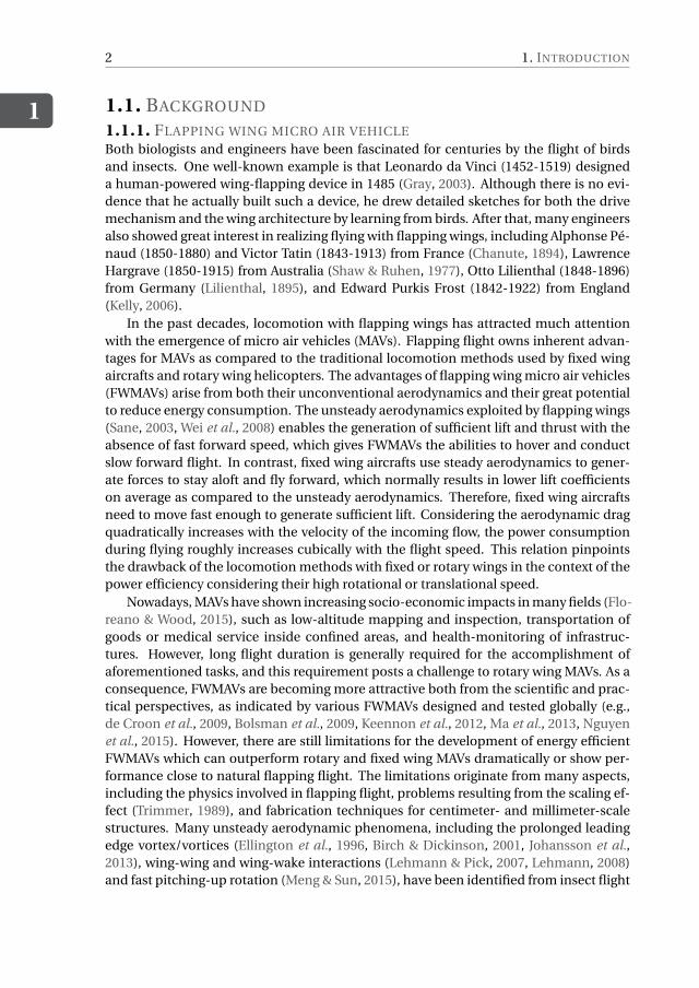
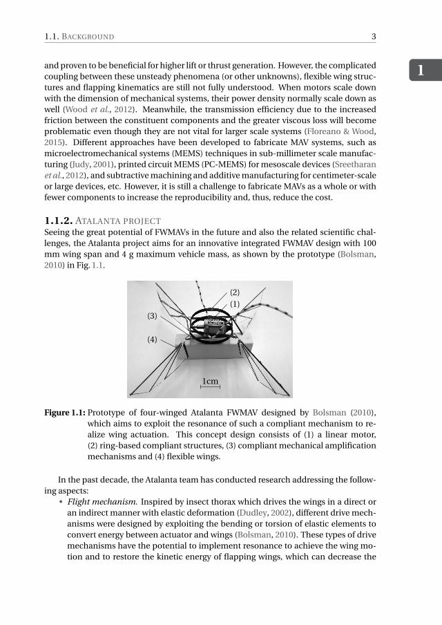
1.1.2. ATALANTA PROJECTSeeing the great potential of FWMAVs in the future and also the related scientific chal-lenges, the Atalanta project aims for an innovative integrated FWMAV design with 100mm wing span and 4 g maximum vehicle mass, as shown by the prototype (Bolsman,2010) in Fig. 1.1.
1cm
(1)(2)
(3)
(4)
Figure 1.1: Prototype of four-winged Atalanta FWMAV designed by Bolsman (2010),which aims to exploit the resonance of such a compliant mechanism to re-alize wing actuation. This concept design consists of (1) a linear motor,(2) ring-based compliant structures, (3) compliant mechanical amplificationmechanisms and (4) flexible wings.
In the past decade, the Atalanta team has conducted research addressing the follow-ing aspects:
• Flight mechanism. Inspired by insect thorax which drives the wings in a direct oran indirect manner with elastic deformation (Dudley, 2002), different drive mech-anisms were designed by exploiting the bending or torsion of elastic elements toconvert energy between actuator and wings (Bolsman, 2010). These types of drivemechanisms have the potential to implement resonance to achieve the wing mo-tion and to restore the kinetic energy of flapping wings, which can decrease the
1
4 1. INTRODUCTION
energy consumption as compared to traditional flight mechanisms using linkagemechanisms and gearboxes.
• Actuator. Traditional electromagnetic motors show a great drop of power densitywhen scaled down. As an alternative, the Atalanta project is working on a chemicalactuator which uses chemical energy directly, like all animals (van Wageningen,2012, van den Heuvel, 2015). One of the highlights of the chemical actuator is thatthe self-weight decreases with the consuming of chemical fuel.
• Sensing. To avoid the large amount of power consumed by image data transmis-sion or onboard image processing, optical flow based flight sensing and controlmethods are being developed to realize the autonomous flight status identifica-tion, obstacle avoidance and object approaching (Selvan, 2014).
• Flight control. The compliant mechanisms used by the Atalanta FWMAVs postnew challenges for the flight control. One developed approach is to control theflapping wing kinematics by changing the dynamic response of the compliant sys-tem which can be realized by tuning the local structural properties (e.g., thickness,Young’s modulus, temperature) (Peters et al., 2016).
1.2. PROBLEM DESCRIPTIONDiverse wing morphologies can be found in the realm of insects (Ellington, 1984a,b,Dudley, 2002, Berman & Wang, 2007). The area, mass and stiffening materials of insectwings are carefully distributed to realize specific wing inertia and flexibility. In contrast,most existing flapping wing designs are either over-simplified in wing morphology (e.g.,de Croon et al., 2009, Bolsman et al., 2009, Keennon et al., 2012, Nguyen et al., 2015) ordirectly duplicate the wing morphology of specific insects (e.g., Tanaka & Wood, 2010, Haet al., 2014). As one of the challenges posted by the Atalanta project, the present work istrying to identify the most influential wing characteristics with respect to the flight per-formance of flapping wings and to achieve new wing designs which can decrease the gapbetween artificial wings for FWMAVs and insect wings, particularly from the perspectiveof energy efficiency.
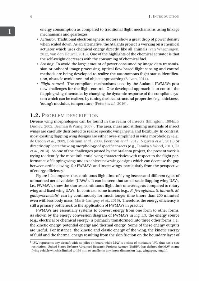
Figure 1.2 compares the continuous flight time of flying insects and different types ofunmanned aerial vehicles (UAVs1). It can be seen that small-scale flapping wing UAVs,i.e., FWMAVs, show the shortest continuous flight time on average as compared to rotarywing and fixed wing UAVs. In contrast, some insects (e.g., R. ferrugineus, S. laurasii, M.galloprovincialis) can fly continuously for much longer time (more than 200 minutes)even with less body mass (Martí-Campoy et al., 2016). Therefore, the energy efficiency isstill a primary bottleneck to the application of FWMAVs in practice.
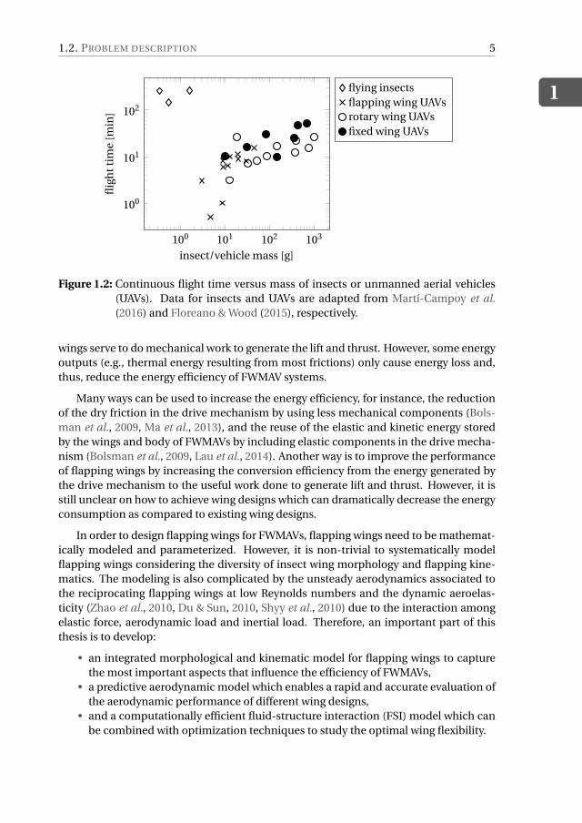
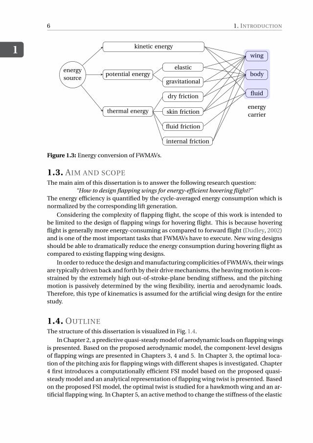
FWMAVs are essentially systems to convert energy from one form to other forms.As shown by the energy conversion diagram of FWMAVs in Fig. 1.3, the energy source(e.g., electrical or chemical energy) is primarily transformed into three other forms, i.e.,the kinetic energy, potential energy and thermal energy. Some of these energy outputsare useful. For instance, the kinetic and elastic energy of the wing, the kinetic energyof fluid and the thermal energy resulting from the skin friction on the boundary layer of
1 UAV represents any aircraft with no pilot on board while MAV is a class of miniature UAV that has a sizerestriction. United States Defense Advanced Research Projects Agency (DARPA) has defined the MAV as anyflying vehicle which is limited to 150 mm or smaller in any linear dimension (e.g., wingspan, length).
1.2. PROBLEM DESCRIPTION
1
5
100 101 102 103
100
101
102
insect/vehicle mass [g]
flig
htt
ime
[min
]
flying insectsflapping wing UAVsrotary wing UAVsfixed wing UAVs
Figure 1.2: Continuous flight time versus mass of insects or unmanned aerial vehicles(UAVs). Data for insects and UAVs are adapted from Martí-Campoy et al.(2016) and Floreano & Wood (2015), respectively.
wings serve to do mechanical work to generate the lift and thrust. However, some energyoutputs (e.g., thermal energy resulting from most frictions) only cause energy loss and,thus, reduce the energy efficiency of FWMAV systems.
Many ways can be used to increase the energy efficiency, for instance, the reductionof the dry friction in the drive mechanism by using less mechanical components (Bols-man et al., 2009, Ma et al., 2013), and the reuse of the elastic and kinetic energy storedby the wings and body of FWMAVs by including elastic components in the drive mecha-nism (Bolsman et al., 2009, Lau et al., 2014). Another way is to improve the performanceof flapping wings by increasing the conversion efficiency from the energy generated bythe drive mechanism to the useful work done to generate lift and thrust. However, it isstill unclear on how to achieve wing designs which can dramatically decrease the energyconsumption as compared to existing wing designs.
In order to design flapping wings for FWMAVs, flapping wings need to be mathemat-ically modeled and parameterized. However, it is non-trivial to systematically modelflapping wings considering the diversity of insect wing morphology and flapping kine-matics. The modeling is also complicated by the unsteady aerodynamics associated tothe reciprocating flapping wings at low Reynolds numbers and the dynamic aeroelas-ticity (Zhao et al., 2010, Du & Sun, 2010, Shyy et al., 2010) due to the interaction amongelastic force, aerodynamic load and inertial load. Therefore, an important part of thisthesis is to develop:
• an integrated morphological and kinematic model for flapping wings to capturethe most important aspects that influence the efficiency of FWMAVs,
• a predictive aerodynamic model which enables a rapid and accurate evaluation ofthe aerodynamic performance of different wing designs,
• and a computationally efficient fluid-structure interaction (FSI) model which canbe combined with optimization techniques to study the optimal wing flexibility.
1
6 1. INTRODUCTION
energysource
kinetic energy
potential energyelastic
gravitational
thermal energy
dry friction
skin friction
fluid friction
internal friction
wing
body
fluid
energycarrier
Figure 1.3: Energy conversion of FWMAVs.
1.3. AIM AND SCOPEThe main aim of this dissertation is to answer the following research question:
“How to design flapping wings for energy-efficient hovering flight?”The energy efficiency is quantified by the cycle-averaged energy consumption which isnormalized by the corresponding lift generation.
Considering the complexity of flapping flight, the scope of this work is intended tobe limited to the design of flapping wings for hovering flight. This is because hoveringflight is generally more energy-consuming as compared to forward flight (Dudley, 2002)and is one of the most important tasks that FWMAVs have to execute. New wing designsshould be able to dramatically reduce the energy consumption during hovering flight ascompared to existing flapping wing designs.
In order to reduce the design and manufacturing complicities of FWMAVs, their wingsare typically driven back and forth by their drive mechanisms, the heaving motion is con-strained by the extremely high out-of-stroke-plane bending stiffness, and the pitchingmotion is passively determined by the wing flexibility, inertia and aerodynamic loads.Therefore, this type of kinematics is assumed for the artificial wing design for the entirestudy.
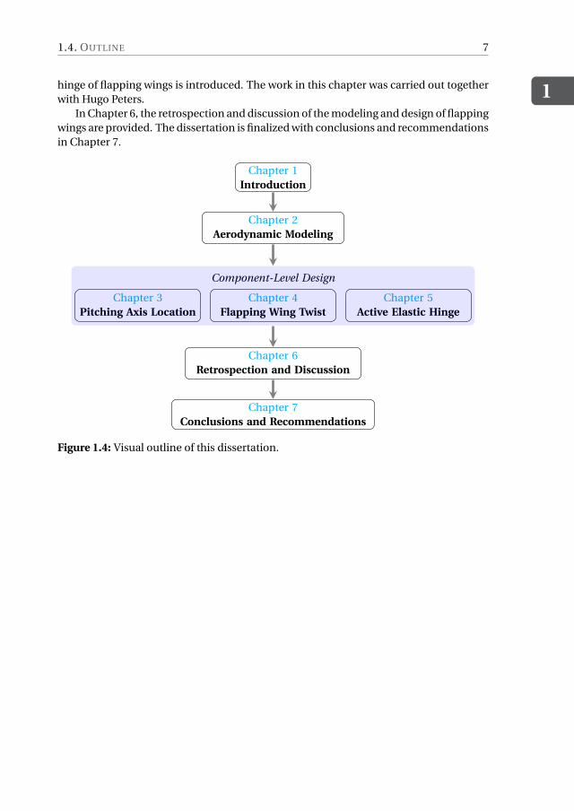
1.4. OUTLINEThe structure of this dissertation is visualized in Fig. 1.4.
In Chapter 2, a predictive quasi-steady model of aerodynamic loads on flapping wingsis presented. Based on the proposed aerodynamic model, the component-level designsof flapping wings are presented in Chapters 3, 4 and 5. In Chapter 3, the optimal loca-tion of the pitching axis for flapping wings with different shapes is investigated. Chapter4 first introduces a computationally efficient FSI model based on the proposed quasi-steady model and an analytical representation of flapping wing twist is presented. Basedon the proposed FSI model, the optimal twist is studied for a hawkmoth wing and an ar-tificial flapping wing. In Chapter 5, an active method to change the stiffness of the elastic
1.4. OUTLINE
1
7
hinge of flapping wings is introduced. The work in this chapter was carried out togetherwith Hugo Peters.
In Chapter 6, the retrospection and discussion of the modeling and design of flappingwings are provided. The dissertation is finalized with conclusions and recommendationsin Chapter 7.
Chapter 1Introduction
Chapter 2Aerodynamic Modeling
Component-Level Design
Chapter 3Pitching Axis Location
Chapter 4Flapping Wing Twist
Chapter 5Active Elastic Hinge
Chapter 6Retrospection and Discussion
Chapter 7Conclusions and Recommendations
Figure 1.4: Visual outline of this dissertation.

2A PREDICTIVE QUASI-STEADY
MODEL OF AERODYNAMIC LOADS
ON FLAPPING WINGS
Quasi-steady aerodynamic models play an important role in evaluating aerodynamic per-formance and conducting design and optimization of flapping wings. Most quasi-steadymodels are aimed at predicting the lift and thrust generation of flapping wings with pre-scribed kinematics. Nevertheless, it is insufficient to limit flapping wings to prescribedkinematics only since passive pitching motion is widely observed in natural flapping flightsand preferred for the wing design of flapping wing micro air vehicles (FWMAVs). In addi-tion to the aerodynamic forces, an accurate estimation of the aerodynamic torque aboutthe pitching axis is required to study the passive pitching motion of flapping flights. Theunsteadiness arising from the wing’s rotation complicates the estimation of the center ofpressure (CP) and the aerodynamic torque within the context of quasi-steady analysis. Al-though there are a few attempts in literature to model the torque analytically, the involvedproblems are still not completely solved.
In this chapter, we present an analytical quasi-steady model by including four aerody-namic loading terms. The loads result from the wing’s translation, rotation, their couplingas well as the added-mass effect. The necessity of including all the four terms in a quasi-steady model in order to predict both the aerodynamic force and torque is demonstrated.Validations indicate a good accuracy of predicting the CP, the aerodynamic loads and thepassive pitching motion for various Reynolds numbers. Moreover, compared to the exist-ing quasi-steady models, the presented model does not rely on any empirical parametersand, thus, is more predictive, which enables application to the shape and kinematics op-timization of flapping wings.
This chapter is based on the paper “Wang, Q., Goosen, J.F.L., van Keulen, F., 2016. A predictive quasi-steadymodel of aerodynamic loads on flapping wings. J. Fluid Mech. 800, 688–719.”
9
2
10 2. A PREDICTIVE QUASI-STEADY AERODYNAMIC MODEL
2.1. INTRODUCTIONOne of the most fascinating features of insects is the reciprocating flapping motion oftheir wings. The flapping motion is generally a combination of wing translation (yaw)and rotation, where the rotation can be further decomposed into wing pitch and roll.The scientific study of insect flight dates back to the time Chabrier (1822) published abook on insect flight and related morphology. However, Hoff (1919) was probably thefirst to analyze the aerodynamics of insect flight with momentum theory which idealizesthe stroke plane as an actuator-disk to continuously impart downward momentum tothe air. Since then, aerodynamic modeling of the force generation by flapping wings, es-pecially in an analytical way, has been a research focus for both biologists and engineers.
Analytical modeling of flapping wing performance can be roughly classified into threegroups: steady-state models, (semi-empirical) quasi-steady models and unsteady mod-els. Steady-state models, including the actuator-disk model (Hoff, 1919), provided us thefirst insight into the average lift generation and power consumption of flapping flightwithout digging into the time course of the transient forces (see Weis-Fogh (1972) andEllington (1984d)). Meanwhile, quasi-steady models were investigated by Osborne (1951)and Ellington (1984c) by taking the change of the angle of attack (AOA) over time andthe velocity variation along the wing span into consideration. Then, with the help ofexperimental studies on dynamically scaled mechanical flapping wings, empirical cor-rections were introduced into quasi-steady models to improve their accuracy. Typicallythese models are refereed to as semi-empirical quasi-steady models (e.g., Dickinsonet al., 1999, Berman & Wang, 2007). Recently, unsteady models attempted to analyticallymodel the unsteady flow phenomena, for instance, the generation and shedding of lead-ing edge vortices (LEVs) and trailing edge vortices (TEVs) (Ansari, 2004, Xia & Mohseni,2013). These models are capable of demonstrating details of the changing flow fieldduring flapping flight with much less computational cost as compared to the numeri-cal simulations which directly solve the governing Navier-Stokes equations. The Kuttacondition is generally enforced at the trailing edge by these unsteady models. However,as pointed out by Ansari et al. (2006), during stroke reversals the fluid is more likely toflow around the trailing edge rather than along it such that the applicability of the Kuttacondition in the conventional sense is questionable.
With the emergence of flapping wing micro air vehicles (FWMAVs), design studies onflapping wings have stimulated research to keep improving existing quasi-steady mod-els by capturing more unsteady characteristics of prescribed flapping motion withoutincreasing the computational cost. Reviews on recent progress can be found in manypapers (e.g., Sane, 2003, Ansari et al., 2006, Shyy et al., 2010). However, the pitching mo-tion of flapping wings of insects, especially during wing reversals, is not always activelycontrolled. Torsional wave along the trailing edge (TE) of a wing traveling from the wingtip to root is considered as a signature of passive or partly passive wing pitching and hasbeen observed on wings of Diptera (Ennos, 1989) and dragonfly (Bergou et al., 2007).To simplify the drive mechanism, wings of FWMAVs are also designed to pitch passively(e.g., de Croon et al., 2009, Bolsman et al., 2009, Ma et al., 2013). In this case, the pitchingmotion is governed by the wing flexibility, inertia and aerodynamic loads.
To study the passive pitching motion and help the wing design, both the aerody-namic force and torque must be calculated. Nevertheless, most existing quasi-steady
2.2. FORMULATION
2
11
pitching axis
R
c
cd
LE
TE
root tip
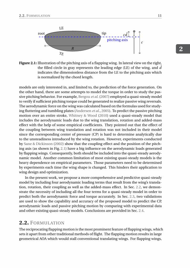
Figure 2.1: Illustration of the pitching axis of a flapping wing. In lateral view on the right,the filled circle in gray represents the leading edge (LE) of the wing, and dindicates the dimensionless distance from the LE to the pitching axis whichis normalized by the chord length.
models are only interested in, and limited to, the prediction of the force generation. Onthe other hand, there are some attempts to model the torque in order to study the pas-sive pitching behavior. For example, Bergou et al. (2007) employed a quasi-steady modelto verify if sufficient pitching torque could be generated to realize passive wing reversals.The aerodynamic force on the wing was calculated based on the formulas used for study-ing fluttering and tumbling plates (Andersen et al., 2005). To predict the passive pitchingmotion over an entire stroke, Whitney & Wood (2010) used a quasi-steady model thatincludes the aerodynamic loads due to the wing translation, rotation and added-masseffect with the help of some empirical coefficients. They pointed out that the effect ofthe coupling between wing translation and rotation was not included in their modelsince the corresponding center of pressure (CP) is hard to determine analytically dueto the unsteadiness introduced by the wing rotation. However, experiments conductedby Sane & Dickinson (2002) show that the coupling effect and the position of the pitch-ing axis (as shown in Fig. 2.1) have a big influence on the aerodynamic loads generatedby flapping wings. Consequently, both should be included into the quasi-steady aerody-namic model. Another common limitation of most existing quasi-steady models is theheavy dependence on empirical parameters. Those parameters need to be determinedby experiments each time the wing shape is changed. This hinders their application towing design and optimization.
In the present work, we propose a more comprehensive and predictive quasi-steadymodel by including four aerodynamic loading terms that result from the wing’s transla-tion, rotation, their coupling as well as the added-mass effect. In Sec. 2.2, we demon-strate the necessity of including all the four terms for a quasi-steady model in order topredict both the aerodynamic force and torque accurately. In Sec. 2.3, two validationsare used to show the capability and accuracy of the proposed model to predict the CP,aerodynamic loads and passive pitching motion by comparing with experimental dataand other existing quasi-steady models. Conclusions are provided in Sec. 2.4.
2.2. FORMULATION
The reciprocating flapping motion is the most prominent feature of flapping wings, whichsets it apart from other traditional methods of flight. The flapping motion results in largegeometrical AOA which would stall conventional translating wings. For flapping wings,
2
12 2. A PREDICTIVE QUASI-STEADY AERODYNAMIC MODEL
generally, the flow starts to separate at the LE after wing reversals, and forms a LEV orLEVs (Johansson et al., 2013). Instead of growing quickly and then shedding into thewake, the LEV on flapping wings generally remains attached over the entire half-strokesfor two possible reasons: (1) the spanwise flow from the wing root to tip removes energyfrom the LEV which limits the growth and the shedding, as shown on hawkmoth wings(Ellington et al., 1996); and (2) due to the downwash flow induced by the tip and wakevortices, the effective AOA decreases and the growth of the LEV is restricted, as indicatedby the wings of Drosophila (Birch & Dickinson, 2001). The prolonged attachment of theLEV assists flapping wings to maintain high lift. This phenomenon makes it more con-venient to analytically model the aerodynamic effect of the attached LEV compared tothe case that the LEV sheds before the pitching reversal.
To analytically predict the unsteady aerodynamic loads on flapping wings, we pre-sume that:
• The flow is incompressible, i.e., the fluid density ρf is regarded as a constant. Thisis justified due to the relative low average wing tip velocity compared to the speedof sound (Sun, 2014).
• The wing is a rigid, flat plate. Wings of some small insects (e.g., fruitfly wings(Ellington, 1999)) and FWMAV wings (Ma et al., 2013) show negligible wing de-formation. Even for wings of larger insects, the enhancement of lift due to wingcamber and twisting is generally less than 10% compared to their rigid counter-parts (Sun, 2014). The wing thickness t is also negligible when compared to theother two dimensions, i.e., the average chord length c and span R (see Fig. 2.1).
• The resultant aerodynamic force acting on the wing is perpendicular to the chordduring the entire stroke. This assumption is supported by three facts: (1) theleading-edge suction force (Sane, 2003) is negligible for a plate with negligiblethickness; (2) the viscous drag on the wing surface is marginal as compared tothe dominant pressure load when moving at a post-stall AOA; (3) the strength ofthe bound circulation, which results in a net force perpendicular to the incomingflow, is negligible as compared to the vorticity-induced circulation (Ford & Babin-sky, 2014).
• A quasi-steady state is assumed for an infinitesimal duration such that the tran-sient loads on the flapping wing are equivalent to those for steady motion at thesame instantaneous translational velocity, angular velocity and AOA.
Considering the variation in the velocity and acceleration along the wing span, theblade element method (BEM) (Osborne, 1951) is used for discretizing the wing into chord-wise strips with finite width. The resultant loads can be calculated by integrating striploads over the entire wing. As a consequence of the quasi-steady assumption, the timedependence of the aerodynamic loads primarily arises from the time-varying kinemat-ics.
2.2.1. FLAPPING KINEMATICS
To describe the kinematics of a rigid flapping wing, three successive rotations, i.e., sweep-ing motion (yaw), heaving motion (roll) and pitching motion (pitch), are used, as illus-trated by the “cans in series” diagram in Fig. 2.2. Four different frames are involved inthese rotations, including an inertial frame xi yizi, two intermediate frames xθyθzθ and
2.2. FORMULATION
2
13
wing
pitchin
g (η)
heaving (θ)
swee
pin
g(φ
)
yizi
xi
yθ
zθ(zi)xθ
yη(yθ)
xη zη
xc(xη)
zcyc
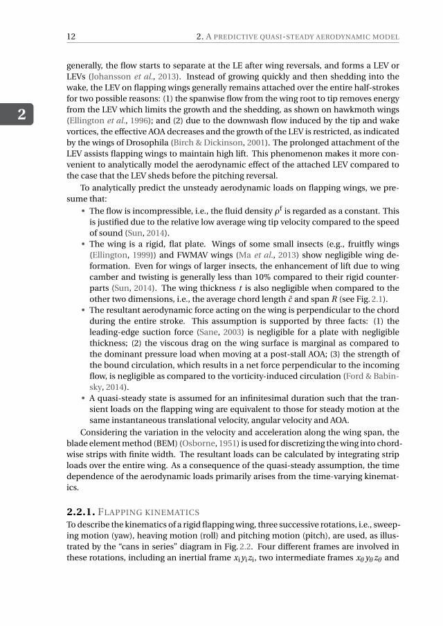
Figure 2.2: Successive wing rotations used to describe the kinematics of a rigid flappingwing, shown using the “cans in series” approach proposed by Schwab & Mei-jaard (2006). Four different frames are involved in these rotations, includingan inertial frame xi yizi, two intermediate frames xθyθzθ and xηyηzη, and aco-rotating frame xc yczc. All these frames share the same origin althoughthey are drawn at various locations.
xηyηzη, and a co-rotating frame xc yczc. The inertial frame xi yizi is fixed at the joint thatconnects the wing to body. Axes xi and yi confine the stroke plane while the zi axis is per-pendicular to this plane and follows the right-hand rule which holds for all the frames.The rotation around the zi axis represents the sweeping motion and results in the inter-mediate frame xθyθzθ. The heaving motion is the rotation around the yθ axis and leadsto another intermediate frame xηyηzη, where the pitching motion is conducted about itsxη axis. Eventually, we get the co-rotating frame xc yczc, which is fixed to and co-rotateswith the wing. Its xc axis coincides with the pitching axis, and the zc axis coincides withthe wing plane and perpendicular to the xc axis. Both the inertial frame xi yizi and theco-rotating frame xc yczc are of particular interest for the study of flapping wing motionand aerodynamic performance. The quasi-steady aerodynamic model presented in thischapter is constructed in the co-rotating frame in order to facilitate the application ofthe BEM, while the lift and drag are generally quantified in the inertial frame.
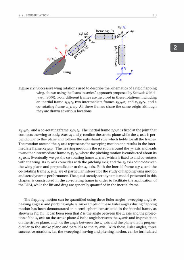
The flapping motion can be quantified using three Euler angles: sweeping angle φ,heaving angle θ and pitching angle η. An example of these Euler angles during flappingmotion has been demonstrated in a semi-sphere constructed in the inertial frame, asshown in Fig. 2.3. It can been seen that φ is the angle between the xi axis and the projec-tion of the xc axis on the stroke plane, θ is the angle between the xc axis and its projectionon the stroke plane, and η is the angle between the zc axis and the plane that is perpen-dicular to the stroke plane and parallels to the xc axis. With these Euler angles, threesuccessive rotations, i.e., the sweeping, heaving and pitching motion, can be formulated
2
14 2. A PREDICTIVE QUASI-STEADY AERODYNAMIC MODEL
xc
yczc
xi
yi
zi
θ
θ
η
φ
tip
TE
LE
Figure 2.3: Two frames and three Euler angles demonstrated in a semi-sphere. Framesxi yizi and xc yczc are fixed to the origin and co-rotates with the wing, respec-tively. Axes xi and yi confine the stroke plane. The small circles indicate thewing tip trajectory (“∞” shape here as an example). The plane constructedby the dashed lines is perpendicular to the stroke plane and parallels to thexc axis. φ, θ and η represent the sweeping, heaving and pitching angle, re-spectively.
as
Rφ =
cosφ −sinφ 0sinφ cosφ 0
0 0 1
,Rθ =
cosθ 0 sinθ0 1 0
−sinθ 0 cosθ
,Rη =
1 0 00 cosη −sinη0 sinη cosη
,
(2.1)respectively.
The quasi-steady model proposed in this work calculates the aerodynamic loadsin the co-rotating frame. Therefore, the flapping velocity and acceleration in the co-rotating frame are required. The angular velocityωc and angular accelerationαc can beobtained by transforming the sweeping and heaving motion from corresponding framesinto the co-rotating frame where the wing pitching motion is described, as in,
ωc = RTηRT
θRTφφezi +RT
ηRTθ θe yθ +RT
η ηexη =
η− φsinθθcosη+ φcosθ sinηφcosηcosθ− θ sinη
, (2.2)
and
αc = ωc =
η− φsinθ− φθcosθφcosθ sinη+ θcosη− ηθ sinη+ φ(ηcosηcosθ− θ sinηsinθ)φcosηcosθ− θ sinη− ηθcosη− φ(ηcosθ sinη+ θcosηsinθ)
, (2.3)
where ezi , e yθ and exη are unit vectors in the zi, yθ and xη directions, respectively.In the co-rotating frame, the translational velocity and acceleration of a point on the
pitching axis with a position vector r = [xc,0,0]T can be calculated by
v c =ωc × r = xc[0,ωzc ,−ωyc ]T, (2.4)
2.2. FORMULATION
2
15
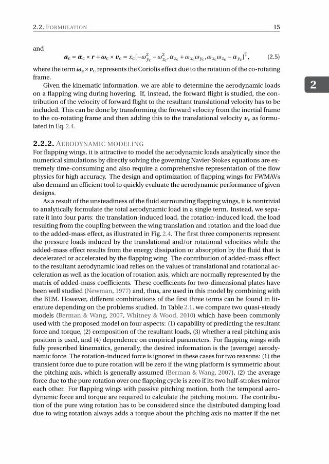
andac =αc × r +ωc ×v c = xc[−ω2
yc−ω2
zc,αzc +ωxcωyc ,ωxcωzc −αyc ]T, (2.5)
where the termωc×v c represents the Coriolis effect due to the rotation of the co-rotatingframe.
Given the kinematic information, we are able to determine the aerodynamic loadson a flapping wing during hovering. If, instead, the forward flight is studied, the con-tribution of the velocity of forward flight to the resultant translational velocity has to beincluded. This can be done by transforming the forward velocity from the inertial frameto the co-rotating frame and then adding this to the translational velocity v c as formu-lated in Eq. 2.4.
2.2.2. AERODYNAMIC MODELINGFor flapping wings, it is attractive to model the aerodynamic loads analytically since thenumerical simulations by directly solving the governing Navier-Stokes equations are ex-tremely time-consuming and also require a comprehensive representation of the flowphysics for high accuracy. The design and optimization of flapping wings for FWMAVsalso demand an efficient tool to quickly evaluate the aerodynamic performance of givendesigns.
As a result of the unsteadiness of the fluid surrounding flapping wings, it is nontrivialto analytically formulate the total aerodynamic load in a single term. Instead, we sepa-rate it into four parts: the translation-induced load, the rotation-induced load, the loadresulting from the coupling between the wing translation and rotation and the load dueto the added-mass effect, as illustrated in Fig. 2.4. The first three components representthe pressure loads induced by the translational and/or rotational velocities while theadded-mass effect results from the energy dissipation or absorption by the fluid that isdecelerated or accelerated by the flapping wing. The contribution of added-mass effectto the resultant aerodynamic load relies on the values of translational and rotational ac-celeration as well as the location of rotation axis, which are normally represented by thematrix of added-mass coefficients. These coefficients for two-dimensional plates havebeen well studied (Newman, 1977) and, thus, are used in this model by combining withthe BEM. However, different combinations of the first three terms can be found in lit-erature depending on the problems studied. In Table 2.1, we compare two quasi-steadymodels (Berman & Wang, 2007, Whitney & Wood, 2010) which have been commonlyused with the proposed model on four aspects: (1) capability of predicting the resultantforce and torque, (2) composition of the resultant loads, (3) whether a real pitching axisposition is used, and (4) dependence on empirical parameters. For flapping wings withfully prescribed kinematics, generally, the desired information is the (average) aerody-namic force. The rotation-induced force is ignored in these cases for two reasons: (1) thetransient force due to pure rotation will be zero if the wing platform is symmetric aboutthe pitching axis, which is generally assumed (Berman & Wang, 2007), (2) the averageforce due to the pure rotation over one flapping cycle is zero if its two half-strokes mirroreach other. For flapping wings with passive pitching motion, both the temporal aero-dynamic force and torque are required to calculate the pitching motion. The contribu-tion of the pure wing rotation has to be considered since the distributed damping loaddue to wing rotation always adds a torque about the pitching axis no matter if the net
2
16 2. A PREDICTIVE QUASI-STEADY AERODYNAMIC MODEL
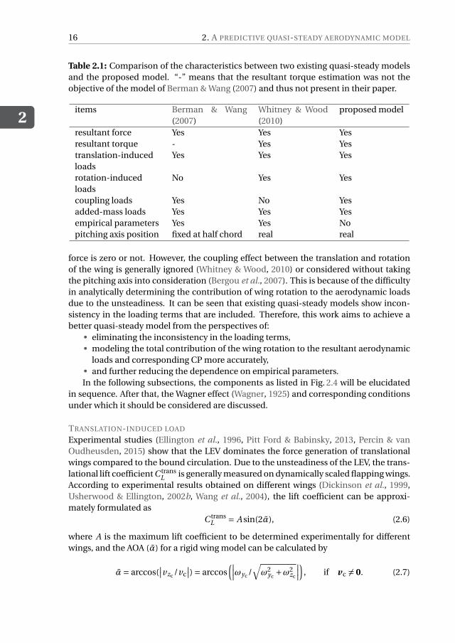
Table 2.1: Comparison of the characteristics between two existing quasi-steady modelsand the proposed model. “-” means that the resultant torque estimation was not theobjective of the model of Berman & Wang (2007) and thus not present in their paper.
items Berman & Wang(2007)
Whitney & Wood(2010)
proposed model
resultant force Yes Yes Yesresultant torque - Yes Yestranslation-inducedloads
Yes Yes Yes
rotation-inducedloads
No Yes Yes
coupling loads Yes No Yesadded-mass loads Yes Yes Yesempirical parameters Yes Yes Nopitching axis position fixed at half chord real real
force is zero or not. However, the coupling effect between the translation and rotationof the wing is generally ignored (Whitney & Wood, 2010) or considered without takingthe pitching axis into consideration (Bergou et al., 2007). This is because of the difficultyin analytically determining the contribution of wing rotation to the aerodynamic loadsdue to the unsteadiness. It can be seen that existing quasi-steady models show incon-sistency in the loading terms that are included. Therefore, this work aims to achieve abetter quasi-steady model from the perspectives of:
• eliminating the inconsistency in the loading terms,• modeling the total contribution of the wing rotation to the resultant aerodynamic
loads and corresponding CP more accurately,• and further reducing the dependence on empirical parameters.In the following subsections, the components as listed in Fig. 2.4 will be elucidated
in sequence. After that, the Wagner effect (Wagner, 1925) and corresponding conditionsunder which it should be considered are discussed.
TRANSLATION-INDUCED LOAD
Experimental studies (Ellington et al., 1996, Pitt Ford & Babinsky, 2013, Percin & vanOudheusden, 2015) show that the LEV dominates the force generation of translationalwings compared to the bound circulation. Due to the unsteadiness of the LEV, the trans-lational lift coefficient C trans
L is generally measured on dynamically scaled flapping wings.According to experimental results obtained on different wings (Dickinson et al., 1999,Usherwood & Ellington, 2002b, Wang et al., 2004), the lift coefficient can be approxi-mately formulated as
C transL = A sin(2α), (2.6)
where A is the maximum lift coefficient to be determined experimentally for differentwings, and the AOA (α) for a rigid wing model can be calculated by
α= arccos(∣∣vzc /vc
∣∣) = arccos(∣∣∣ωyc /
√ω2
yc+ω2
zc
∣∣∣)
, if v c 6= 0. (2.7)
2.2. FORMULATION
2
17
yc
zc
vc ac
ωxcαxc
F aeroyc
totalaerodynamic
load
⇒ vc
F transyc
(1)translation-
induced load
+
ωxcF rot
yc
(2)rotation-
induced load
+vc
vzcωxcF coupl
yc
(3)coupling
load
+ac
αxc
F amyc
(4)added-mass
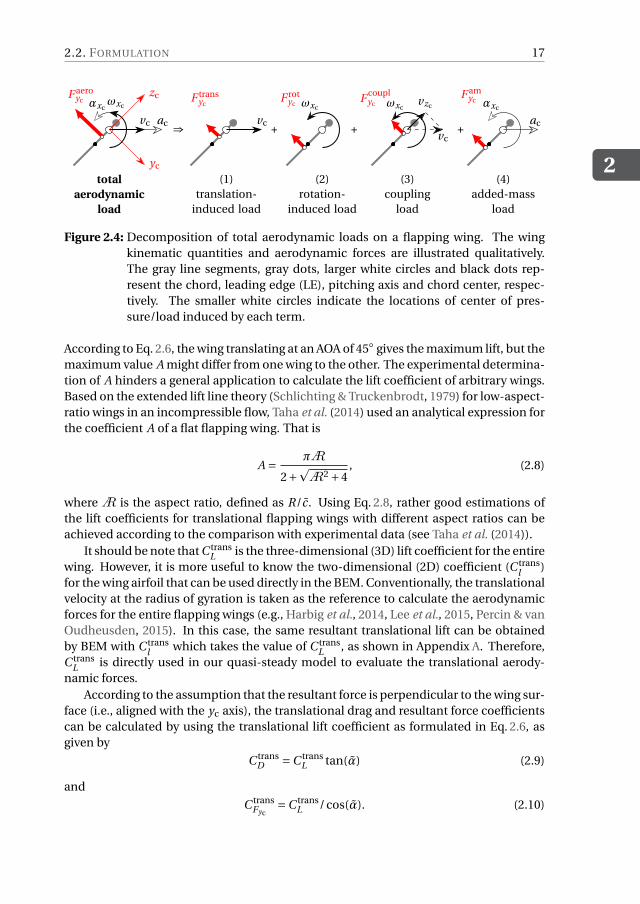
load
Figure 2.4: Decomposition of total aerodynamic loads on a flapping wing. The wingkinematic quantities and aerodynamic forces are illustrated qualitatively.The gray line segments, gray dots, larger white circles and black dots rep-resent the chord, leading edge (LE), pitching axis and chord center, respec-tively. The smaller white circles indicate the locations of center of pres-sure/load induced by each term.
According to Eq. 2.6, the wing translating at an AOA of 45◦ gives the maximum lift, but themaximum value A might differ from one wing to the other. The experimental determina-tion of A hinders a general application to calculate the lift coefficient of arbitrary wings.Based on the extended lift line theory (Schlichting & Truckenbrodt, 1979) for low-aspect-ratio wings in an incompressible flow, Taha et al. (2014) used an analytical expression forthe coefficient A of a flat flapping wing. That is
A = πA
2+pA2 +4
, (2.8)
whereA is the aspect ratio, defined as R/c. Using Eq. 2.8, rather good estimations ofthe lift coefficients for translational flapping wings with different aspect ratios can beachieved according to the comparison with experimental data (see Taha et al. (2014)).
It should be note that C transL is the three-dimensional (3D) lift coefficient for the entire
wing. However, it is more useful to know the two-dimensional (2D) coefficient (C transl )
for the wing airfoil that can be used directly in the BEM. Conventionally, the translationalvelocity at the radius of gyration is taken as the reference to calculate the aerodynamicforces for the entire flapping wings (e.g., Harbig et al., 2014, Lee et al., 2015, Percin & vanOudheusden, 2015). In this case, the same resultant translational lift can be obtainedby BEM with C trans
l which takes the value of C transL , as shown in Appendix A. Therefore,
C transL is directly used in our quasi-steady model to evaluate the translational aerody-
namic forces.According to the assumption that the resultant force is perpendicular to the wing sur-
face (i.e., aligned with the yc axis), the translational drag and resultant force coefficientscan be calculated by using the translational lift coefficient as formulated in Eq. 2.6, asgiven by
C transD =C trans
L tan(α) (2.9)
and
C transFyc
=C transL /cos(α). (2.10)
2
18 2. A PREDICTIVE QUASI-STEADY AERODYNAMIC MODEL
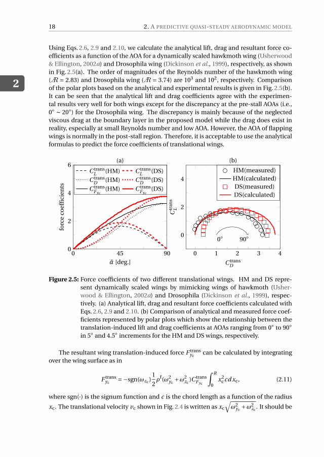
Using Eqs. 2.6, 2.9 and 2.10, we calculate the analytical lift, drag and resultant force co-efficients as a function of the AOA for a dynamically scaled hawkmoth wing (Usherwood& Ellington, 2002a) and Drosophila wing (Dickinson et al., 1999), respectively, as shownin Fig. 2.5(a). The order of magnitudes of the Reynolds number of the hawkmoth wing(A = 2.83) and Drosophila wing (A = 3.74) are 103 and 102, respectively. Comparisonof the polar plots based on the analytical and experimental results is given in Fig. 2.5(b).It can be seen that the analytical lift and drag coefficients agree with the experimen-tal results very well for both wings except for the discrepancy at the pre-stall AOAs (i.e.,0◦ ∼ 20◦) for the Drosophila wing. The discrepancy is mainly because of the neglectedviscous drag at the boundary layer in the proposed model while the drag does exist inreality, especially at small Reynolds number and low AOA. However, the AOA of flappingwings is normally in the post-stall region. Therefore, it is acceptable to use the analyticalformulas to predict the force coefficients of translational wings.
0 45 900
2
4
6
α [deg.]
forc
eco
effi
cien
ts
(a)
C transL (HM) C trans
L (DS)
C transD (HM) C trans
D (DS)
C transFyc
(HM) C transFyc
(DS)
0 1 2 3 4
0
2
4
0◦ 90◦
C transD
Ctr
ans
L
(b)
HM(measured)HM(calculated)DS(measured)DS(calculated)
Figure 2.5: Force coefficients of two different translational wings. HM and DS repre-sent dynamically scaled wings by mimicking wings of hawkmoth (Usher-wood & Ellington, 2002a) and Drosophila (Dickinson et al., 1999), respec-tively. (a) Analytical lift, drag and resultant force coefficients calculated withEqs. 2.6, 2.9 and 2.10. (b) Comparison of analytical and measured force coef-ficients represented by polar plots which show the relationship between thetranslation-induced lift and drag coefficients at AOAs ranging from 0◦ to 90◦
in 5◦ and 4.5◦ increments for the HM and DS wings, respectively.
The resultant wing translation-induced force F transyc
can be calculated by integratingover the wing surface as in
F transyc
=−sgn(ωzc )1
2ρf(ω2
yc+ω2
zc)C trans
Fyc
∫ R
0x2
c cd xc, (2.11)
where sgn(·) is the signum function and c is the chord length as a function of the radius
xc. The translational velocity vc shown in Fig. 2.4 is written as xc
√ω2
yc+ω2
zc. It should be
2.2. FORMULATION
2
19
noted that the angular velocity has been taken out of the integration based on the rigidwing assumption.
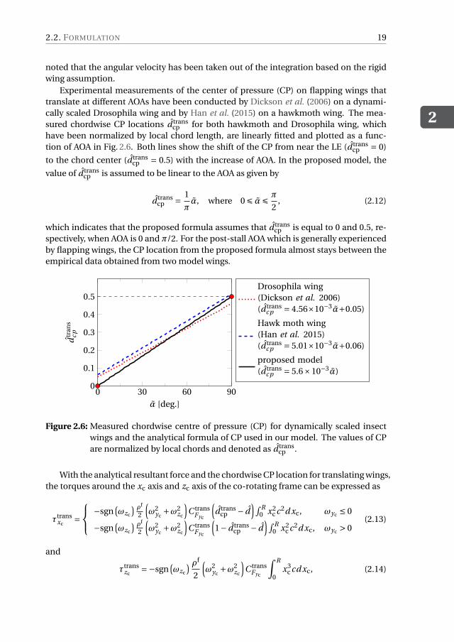
Experimental measurements of the center of pressure (CP) on flapping wings thattranslate at different AOAs have been conducted by Dickson et al. (2006) on a dynami-cally scaled Drosophila wing and by Han et al. (2015) on a hawkmoth wing. The mea-sured chordwise CP locations d trans
cp for both hawkmoth and Drosophila wing, whichhave been normalized by local chord length, are linearly fitted and plotted as a func-tion of AOA in Fig. 2.6. Both lines show the shift of the CP from near the LE (d trans
cp = 0)
to the chord center (d transcp = 0.5) with the increase of AOA. In the proposed model, the
value of d transcp is assumed to be linear to the AOA as given by
d transcp = 1
πα, where 0 É αÉ π
2, (2.12)
which indicates that the proposed formula assumes that d transcp is equal to 0 and 0.5, re-
spectively, when AOA is 0 and π/2. For the post-stall AOA which is generally experiencedby flapping wings, the CP location from the proposed formula almost stays between theempirical data obtained from two model wings.
0 30 60 900
0.1
0.2
0.3
0.4
0.5
α [deg.]
dtr
ans
cp
Drosophila wing(Dickson et al. 2006)(d trans
cp = 4.56×10⁻³α+0.05)
Hawk moth wing(Han et al. 2015)(d trans
cp = 5.01×10⁻³α+0.06)
proposed model(d trans
cp = 5.6×10⁻³α)
Figure 2.6: Measured chordwise centre of pressure (CP) for dynamically scaled insectwings and the analytical formula of CP used in our model. The values of CPare normalized by local chords and denoted as d trans
cp .
With the analytical resultant force and the chordwise CP location for translating wings,the torques around the xc axis and zc axis of the co-rotating frame can be expressed as
τtransxc
=
−sgn(ωzc
) ρf
2
(ω2
yc+ω2
zc
)C trans
Fyc
(d trans
cp − d)∫ R
0 x2c c2d xc, ωyc ≤ 0
−sgn(ωzc
) ρf
2
(ω2
yc+ω2
zc
)C trans
Fyc
(1− d trans
cp − d)∫ R
0 x2c c2d xc, ωyc > 0
(2.13)
and
τtranszc
=−sgn(ωzc
) ρf
2
(ω2
yc+ω2
zc
)C trans
Fyc
∫ R
0x3
c cd xc, (2.14)
2
20 2. A PREDICTIVE QUASI-STEADY AERODYNAMIC MODEL
where d is the normalized distance between the LE and the pitching axis (see Fig. 2.1),and the negative and positive values of ωyc mean that the translational velocity compo-nent vzc (=−xcωyc ) points at the LE and TE, respectively. When ωyc > 0, the real AOA ishigher than 90◦ which is not covered by the analytical model for AOA as shown in Fig. 2.6.This situation is handled by taking the TE as the LE, then the AOA becomes less than 90◦.The torque about yc axis is zero since the resultant force is assumed to be perpendicularto the wing.
The translation-induced loads have been analytically represented while taking ac-count of the influence ofA. This allows further application to study the wing shapeinfluence in an analytical manner.
ROTATION-INDUCED LOAD
When a wing rotates about an arbitrary axis in a medium, it experiences distributedloads. Although the resultant force is zero if the wing is symmetric about its rotationaxis, the resultant torque about the rotation axis is non-zero. Therefore, it is necessary toinclude this rotation-induced load in the quasi-steady model to correctly calculate theaerodynamic torque. In fact, this loading term is excluded by most existing quasi-steadymodels.
To calculate this load using BEM, the wing has to be discretized into chordwise stripsfirst. For a rotating wing, different velocities are induced in the chordwise direction (=−zcωxc ), of which the amplitude linearly increases with the distance from the pitchingaxis. The chordwise velocity gradient requires the discretization of each chordwise stripas well. Consequently, the resultant rotation-induced force is calculated by integratingthe load on each infinitesimal area (i.e., d xcd zc) over the entire wing surface, as in
F rotyc
= ρf
2ωxc |ωxc |C rot
D
∫ R
0
∫ dc
dc−czc |zc|d zcd xc, (2.15)
where C rotD is the rotational damping coefficient, dc−c and dc are the coordinates of the
wing’s trailing edge (TE) and leading edge (LE) in the zc direction, respectively. Mean-while, the resultant torques around axes xc and zc are calculated by
τrotxc
=−ρf
2ωxc |ωxc |C rot
D
∫ R
0
∫ dc
dc−c|zc|3 d zcd xc, (2.16)
and
τrotzc
= ρf
2ωxc |ωxc |C rot
D
∫ R
0
∫ dc
dc−czc |zc|xcd zcd xc. (2.17)
This discretization approach was also used by Andersen et al. (2005) with a value of 2.0for C rot
D on a tumbling plate and by Whitney & Wood (2010) with a value of 5.0 for flap-ping wings to achieve a better agreement between theoretical and experimental results.It is necessary to generalize this coefficient to enable the application for different flap-ping wings. The damping load on a rotating plate is analogous to the load acting on aplate that is placed vertically in a flow with varying incoming velocities from the top tobottom. The latter is basically the case for a translational wing at an angle of attack of90◦. However, it is questionable if it is sufficient to use the traditional drag coefficient for
2.2. FORMULATION
2
21
a pure translating plate normal to flow (≈ 2 for a flat plate at Re = 105 (Anderson, 2010)).During the wing reversals of flapping motion, the sweeping motion is almost seized butthe pitching velocity is nearly maximized. In this case, the pure rotational load domi-nates the aerodynamic loading which is still influenced by the flow field induced by thepast sweeping motion. In this situation, it is more correct to use the translational dragcoefficient C trans
D for a sweeping wing (see Eq. 2.9) when AOA is equal to 90◦ as the rota-tional damping coefficient, i.e.,
C rotD =C trans
D (α= π
2) = 2πA
2+pA2 +4
, (2.18)
which normally leads to higher damping coefficients (e.g., C rotD = 3.36 whenA = 3) as
compared to the drag coefficient for a pure translating plate normal to flow.To avoid alternating the LE during flapping, which increases the power consumption,
the pitching axes of flapping wings are generally located between the LE and the centerline (Berman & Wang, 2007). The CP location of the load induced by the pure rotation,which is defined as the local-chord-length-normalized distance from the LE to the CP,can be determined by
d rotcp =−3
4
(d −1)4 + d 4
(d −1)3 + d 3+ d , where 0 É d < 0.5, (2.19)
which implies that the CP moves from 3/4 chord to infinity while the pitching axis movesfrom the LE to the chord centre.
COUPLING LOAD
Although the translation- and rotation-induced loads have been modeled analyticallyand separately, they are insufficient to represent the loads on the wing conducting trans-lation and rotation simultaneously because of the nonlinearity introduced by the fluid-wing interaction. Considering a wing whose planform is symmetric about its pitch-ing axis and moving with constant translational and rotational velocities, the resultantrotation-induced force F rot
ycis equal to zero. The resultant force, therefore, should be
equal to the translational force F transyc
for a linear system assumption. However, for thiscase, the experiment conducted by Sane & Dickinson (2002) reported higher resultantforce compared to F trans
yc. This additional force is explained by the coupling effect be-
tween the wing translation and rotation.Traditionally, the coupling load on a plate with translational velocity v , rotational
angular velocity ωxc , chord c and unit span is formulated as
F coupltrad = ρfv C couplωxc c2
(3
4− d
)
︸ ︷︷ ︸rotationalcirculation
, (2.20)
where C coupl is a constant coupling coefficient equal to π. The term was first includedinto a quasi-steady model for flapping wings by Ellington (1984c) to reflect the con-tribution of wing rotation on the aerodynamic force. Since then, this term is widelyused in quasi-steady analysis (Dickinson et al., 1999, Sane & Dickinson, 2002, Nabawy &
2
22 2. A PREDICTIVE QUASI-STEADY AERODYNAMIC MODEL
Crowther, 2014) for different types of insect wings. It is generally assumed that the con-tribution of the wing rotation can be represented by this single coupling term withoutconsidering the load due to the pure wing rotation. However, there are some limitationsfor the coupling term to fully represent the rotational effect. Firstly, the coupling coeffi-cient C coupl in Eq. 2.20 is a constant, but experiments (Sane & Dickinson, 2002, Han et al.,2015) have shown its dependency on the ratio between the translational velocity v androtational angular velocityωxc . Secondly, the influence of the wing rotation on the loca-tion of center of pressure (CP) can not be reflected purely by the coupling term presentedin Eq. 2.20. In fact, according to the experimental results from Han et al. (2015), the tra-jectories of CP locations for different AOAs are different when the wing is pitching up atdifferent velocities even though the sweeping motion is maintained. Thirdly, this singleterm fails to predict the aerodynamic force due to wing rotation when the pitching axis
is at 3/4 chord (F coupltrad = 0 for this case). Fourthly, at the start and end of each half-stroke,
the rotational torque predicted by Eq. 2.20 is small as a result of small translational ve-locity v . However, the aerodynamic torque about the pitching axis at these moments canbe considerable due to the pure wing rotation, as shown in subsection 2.2.2.
v
yc
zcΓrot
⇒ v
vyc
Γrot
+ v
vzc
Γrot
Figure 2.7: Decomposition of the coupling effect between the wing translation and ro-tation. Γrot represents the circulation induced by the wing rotation.
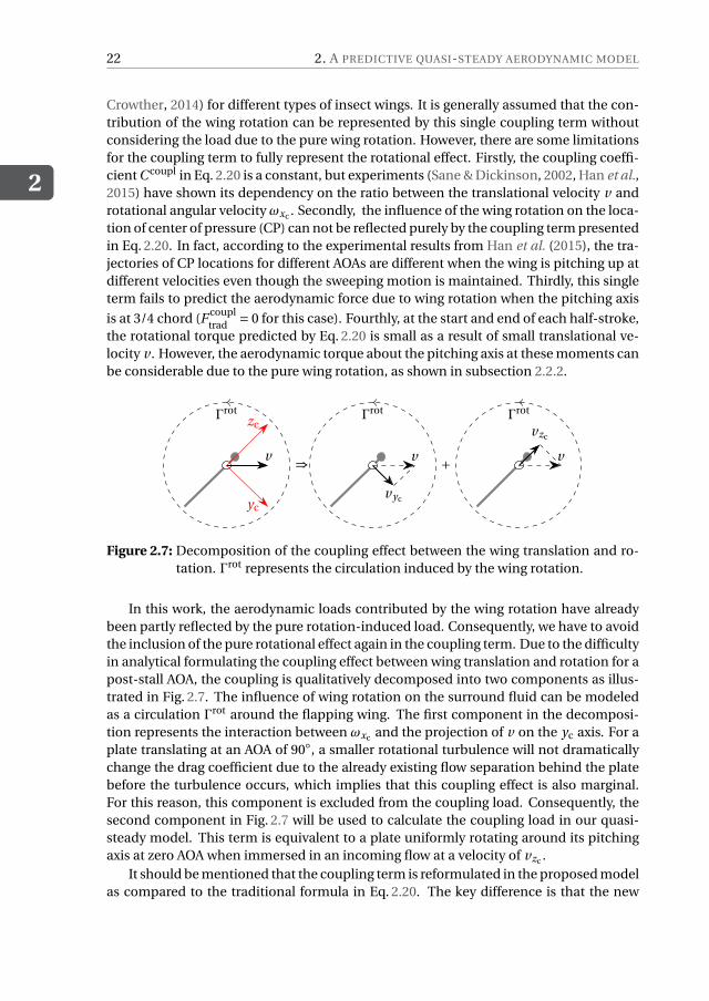
In this work, the aerodynamic loads contributed by the wing rotation have alreadybeen partly reflected by the pure rotation-induced load. Consequently, we have to avoidthe inclusion of the pure rotational effect again in the coupling term. Due to the difficultyin analytical formulating the coupling effect between wing translation and rotation for apost-stall AOA, the coupling is qualitatively decomposed into two components as illus-trated in Fig. 2.7. The influence of wing rotation on the surround fluid can be modeledas a circulation Γrot around the flapping wing. The first component in the decomposi-tion represents the interaction between ωxc and the projection of v on the yc axis. For aplate translating at an AOA of 90◦, a smaller rotational turbulence will not dramaticallychange the drag coefficient due to the already existing flow separation behind the platebefore the turbulence occurs, which implies that this coupling effect is also marginal.For this reason, this component is excluded from the coupling load. Consequently, thesecond component in Fig. 2.7 will be used to calculate the coupling load in our quasi-steady model. This term is equivalent to a plate uniformly rotating around its pitchingaxis at zero AOA when immersed in an incoming flow at a velocity of vzc .
It should be mentioned that the coupling term is reformulated in the proposed modelas compared to the traditional formula in Eq. 2.20. The key difference is that the new
2.2. FORMULATION
2
23
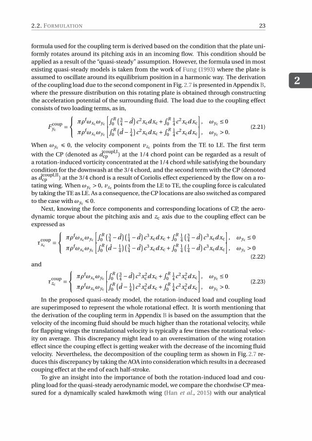
formula used for the coupling term is derived based on the condition that the plate uni-formly rotates around its pitching axis in an incoming flow. This condition should beapplied as a result of the “quasi-steady" assumption. However, the formula used in mostexisting quasi-steady models is taken from the work of Fung (1993) where the plate isassumed to oscillate around its equilibrium position in a harmonic way. The derivationof the coupling load due to the second component in Fig. 2.7 is presented in Appendix B,where the pressure distribution on this rotating plate is obtained through constructingthe acceleration potential of the surrounding fluid. The load due to the coupling effectconsists of two loading terms, as in,
F coupyc
=
πρfωxcωyc
[∫ R0
( 34 − d
)c2xcd xc +
∫ R0
14 c2xcd xc
], ωyc ≤ 0
πρfωxcωyc
[∫ R0
(d − 1
4
)c2xcd xc +
∫ R0
14 c2xcd xc
], ωyc > 0.
(2.21)
When ωyc É 0, the velocity component vzc points from the TE to LE. The first term
with the CP (denoted as d coupl,Icp ) at the 1/4 chord point can be regarded as a result of
a rotation-induced vorticity concentrated at the 1/4 chord while satisfying the boundarycondition for the downwash at the 3/4 chord, and the second term with the CP (denotedas d coupl,II
cp ) at the 3/4 chord is a result of Coriolis effect experienced by the flow on a ro-tating wing. When ωyc > 0, vzc points from the LE to TE, the coupling force is calculatedby taking the TE as LE. As a consequence, the CP locations are also switched as comparedto the case with ωyc É 0.
Next, knowing the force components and corresponding locations of CP, the aero-dynamic torque about the pitching axis and zc axis due to the coupling effect can beexpressed as
τcoupxc
=
πρfωxcωyc
[∫ R0
( 34 − d
)( 14 − d
)c3xcd xc +
∫ R0
14
( 34 − d
)c3xcd xc
], ωyc ≤ 0
πρfωxcωyc
[∫ R0
(d − 1
4
)( 34 − d
)c3xcd xc +
∫ R0
14
( 14 − d
)c3xcd xc
], ωyc > 0
(2.22)and
τcoupzc
=
πρfωxcωyc
[∫ R0
( 34 − d
)c2x2
c d xc +∫ R
014 c2x2
c d xc
], ωyc ≤ 0
πρfωxcωyc
[∫ R0
(d − 1
4
)c2x2
c d xc +∫ R
014 c2x2
c d xc
], ωyc > 0.
(2.23)
In the proposed quasi-steady model, the rotation-induced load and coupling loadare superimposed to represent the whole rotational effect. It is worth mentioning thatthe derivation of the coupling term in Appendix B is based on the assumption that thevelocity of the incoming fluid should be much higher than the rotational velocity, whilefor flapping wings the translational velocity is typically a few times the rotational veloc-ity on average. This discrepancy might lead to an overestimation of the wing rotationeffect since the couping effect is getting weaker with the decrease of the incoming fluidvelocity. Nevertheless, the decomposition of the coupling term as shown in Fig. 2.7 re-duces this discrepancy by taking the AOA into consideration which results in a decreasedcouping effect at the end of each half-stroke.
To give an insight into the importance of both the rotation-induced load and cou-pling load for the quasi-steady aerodynamic model, we compare the chordwise CP mea-sured for a dynamically scaled hawkmoth wing (Han et al., 2015) with our analytical
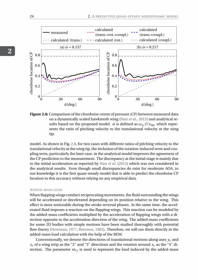
2
24 2. A PREDICTIVE QUASI-STEADY AERODYNAMIC MODEL
0 30 60 900
0.2
0.4
0.6
0.8
α[deg.]
cho
rdw
ise
loca
tio
no
fCP
(a) ω= 0.157
0 30 60 900
0.2
0.4
0.6
0.8
α[deg.]ch
ord
wis
elo
cati
on
ofC
P
(b) ω= 0.217
measuredcalculated(trans.+rot.+coupl.)
calculated(trans.+coupl.)
calculated (trans.) calculated (rot.) calculated (coupl.)
Figure 2.8: Comparison of the chordwise centre of pressure (CP) between measured dataon a dynamically scaled hawkmoth wing (Han et al., 2015) and analytical re-sults based on the proposed model. ω is defined as ωxc c/vtip, which repre-sents the ratio of pitching velocity to the translational velocity at the wingtip.
model. As shown in Fig. 2.8, for two cases with different ratios of pitching velocity to thetranslational velocity at the wing tip, the inclusion of the rotation-induced term and cou-pling term, particularly the later case, in the analytical model improves the agreement ofthe CP prediction to the measurement. The discrepancy at the initial stage is mainly dueto the initial acceleration as reported by Han et al. (2015) which was not considered inthe analytical results. Even though small discrepancies do exist for moderate AOA, toour knowledge it is the first quasi-steady model that is able to predict the chordwise CPlocation to this accuracy without relying on any empirical data.
ADDED-MASS LOAD
When flapping wings conduct reciprocating movements, the fluid surrounding the wingswill be accelerated or decelerated depending on its position relative to the wing. Thiseffect is most noticeable during the stroke reversal phases. At the same time, the accel-erated fluid imposes a reaction on the flapping wings. This reaction can be modeled bythe added-mass coefficients multiplied by the acceleration of flapping wings with a di-rection opposite to the acceleration direction of the wing. The added-mass coefficientsfor some 2D bodies with simple motions have been studied thoroughly with potentialflow theory (Newman, 1977, Brennen, 1982). Therefore, we will use them directly in theadded-mass load calculation with the help of the BEM.
Conventionally, we denote the directions of translational motions along axes yc andzc of a wing strip as the “2" and “3" directions and the rotation around xc as the “4" di-rection. The parameter mi j is used to represent the load induced by the added-mass
2.2. FORMULATION
2
25
effect in the i direction due to a unit acceleration in the j direction. Since the thicknessof flapping wings studied and the viscous drag are negligible, all the added-mass coeffi-cients related to the motion in the “3" direction are ignored. Therefore, for a wing stripwith chord length c, unit width and its pitching axis with a normalized offset d from theLE, the matrix of added-mass coefficients can be expressed as
M =[
m22 m24
m42 m44
]= π
4ρfc2
[1 c(1/2− d0)
c(1/2− d0) 132 c2 + c2(1/2− d0)2
]. (2.24)
Subsequently, the loads due to added-mass effect can be calculated by
[F am
yc,τam
xc
]T=−
∫ R
0M
[ayc ,αxc
]T d xc, (2.25)
where ayc is the translational acceleration in the yc direction and αxc is the rotationalacceleration around the xc direction. The total torque about the zc axis can be easilycalculated by integrating along the span. Additionally, it can be found that the centers ofpressure induced by the translational and rotational motion, denoted as d am,I
cp and d am,IIcp ,
are located at the half and (9−16d)/(16−32d) chord, respectively.
WAGNER EFFECT
For a wing immersed in an incompressible fluid with a small AOA, Wagner (1925) pro-posed that the bound circulation around it does not immediately reach its steady-statevalue if it starts impulsively from rest to a uniform velocity. Instead, the correspond-ing circulatory force increases slowly to its steady-state value according to the Wagner’sfunction. This Wagner effect was experimentally confirmed by Walker (1931) at Re =1.4×10⁵. Sane (2003) attributed it to two reasons: (1) Kutta condition takes time to es-tablish, (2) TEVs are generated and shed gradually. For an immediately started trans-lating plate at two different post-stall AOAs (15◦ and 45◦), an experiment at Re = 3×10⁴
conducted by Ford & Babinsky (2014) indicates that the increase of circulation surround-ing the plate shows a good agreement with the circulation growth proposed by Wagner(1925), although the circulation is dominated by the LEV instead of the bound circu-lation. However, there is no strong evidence showing that the Wagner effect has a no-ticeable influence on wings translating at post-stall AOAs in the intermediate Re regime(10 < Re < 1000) (Dickinson & Götz, 1993). Especially, for the study of aerodynamics ofinsects flights, the Wagner effect is generally ignored due to the rapidly formed LEV as aresult of high AOAs over the entire stroke and low Reynolds numbers.
Apparently, there is no standard yet to determine if the Wagner effect has to be in-cluded or not, and the decision has to be made based on both Re and the type of wingmotion. In this work, if the Wagner effect is included, all the circulatory loads will bemultiplied by an approximate formula of Wagner’s function given by Jones (1940),
Φ(t∗) = 1−0.165e−0.0455t∗ −0.335e−0.300t∗ , (2.26)
where t∗ is a non-dimensional quantity defined as the number of semi-chords the winghas traveled.
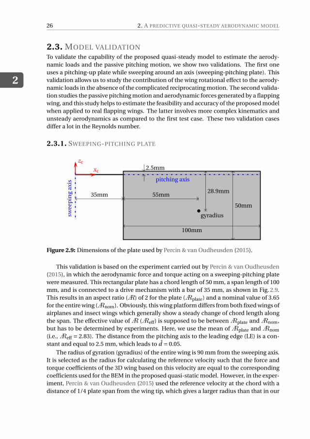
2
26 2. A PREDICTIVE QUASI-STEADY AERODYNAMIC MODEL
2.3. MODEL VALIDATIONTo validate the capability of the proposed quasi-steady model to estimate the aerody-namic loads and the passive pitching motion, we show two validations. The first oneuses a pitching-up plate while sweeping around an axis (sweeping-pitching plate). Thisvalidation allows us to study the contribution of the wing rotational effect to the aerody-namic loads in the absence of the complicated reciprocating motion. The second valida-tion studies the passive pitching motion and aerodynamic forces generated by a flappingwing, and this study helps to estimate the feasibility and accuracy of the proposed modelwhen applied to real flapping wings. The latter involves more complex kinematics andunsteady aerodynamics as compared to the first test case. These two validation casesdiffer a lot in the Reynolds number.
2.3.1. SWEEPING-PITCHING PLATE
gyradius
xc
zc
pitching axis
swee
pin
gax
is
35mm 55mm28.9mm
100mm
50mm
2.5mm
Figure 2.9: Dimensions of the plate used by Percin & van Oudheusden (2015).
This validation is based on the experiment carried out by Percin & van Oudheusden(2015), in which the aerodynamic force and torque acting on a sweeping-pitching platewere measured. This rectangular plate has a chord length of 50 mm, a span length of 100mm, and is connected to a drive mechanism with a bar of 35 mm, as shown in Fig. 2.9.This results in an aspect ratio (A) of 2 for the plate (Aplate) and a nominal value of 3.65for the entire wing (Anom). Obviously, this wing platform differs from both fixed wings ofairplanes and insect wings which generally show a steady change of chord length alongthe span. The effective value ofA (Aeff) is supposed to be betweenAplate andAnom,but has to be determined by experiments. Here, we use the mean ofAplate andAnom
(i.e.,Aeff = 2.83). The distance from the pitching axis to the leading edge (LE) is a con-stant and equal to 2.5 mm, which leads to d = 0.05.
The radius of gyration (gyradius) of the entire wing is 90 mm from the sweeping axis.It is selected as the radius for calculating the reference velocity such that the force andtorque coefficients of the 3D wing based on this velocity are equal to the correspondingcoefficients used for the BEM in the proposed quasi-static model. However, in the exper-iment, Percin & van Oudheusden (2015) used the reference velocity at the chord with adistance of 1/4 plate span from the wing tip, which gives a larger radius than that in our
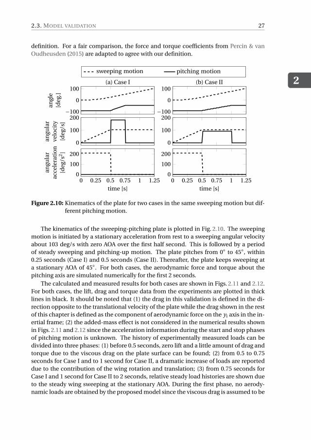
2.3. MODEL VALIDATION
2
27
definition. For a fair comparison, the force and torque coefficients from Percin & vanOudheusden (2015) are adapted to agree with our definition.
−100
0
100
angl
e[d
eg.]
(a) Case I
−100
0
100(b) Case II
sweeping motion pitching motion
0
100
200
angu
lar
velo
city
[deg
/s]
0
100
200
0 0.25 0.5 0.75 1 1.250
100
200
time [s]
angu
lar
acce
lera
tio
n[d
eg/s
2]
0 0.25 0.5 0.75 1 1.250
100
200
time [s]
Figure 2.10: Kinematics of the plate for two cases in the same sweeping motion but dif-ferent pitching motion.
The kinematics of the sweeping-pitching plate is plotted in Fig. 2.10. The sweepingmotion is initiated by a stationary acceleration from rest to a sweeping angular velocityabout 103 deg/s with zero AOA over the first half second. This is followed by a periodof steady sweeping and pitching-up motion. The plate pitches from 0◦ to 45◦, within0.25 seconds (Case I) and 0.5 seconds (Case II). Thereafter, the plate keeps sweeping ata stationary AOA of 45◦. For both cases, the aerodynamic force and torque about thepitching axis are simulated numerically for the first 2 seconds.
The calculated and measured results for both cases are shown in Figs. 2.11 and 2.12.For both cases, the lift, drag and torque data from the experiments are plotted in thicklines in black. It should be noted that (1) the drag in this validation is defined in the di-rection opposite to the translational velocity of the plate while the drag shown in the restof this chapter is defined as the component of aerodynamic force on the yi axis in the in-ertial frame; (2) the added-mass effect is not considered in the numerical results shownin Figs. 2.11 and 2.12 since the acceleration information during the start and stop phasesof pitching motion is unknown. The history of experimentally measured loads can bedivided into three phases: (1) before 0.5 seconds, zero lift and a little amount of drag andtorque due to the viscous drag on the plate surface can be found; (2) from 0.5 to 0.75seconds for Case I and to 1 second for Case II, a dramatic increase of loads are reporteddue to the contribution of the wing rotation and translation; (3) from 0.75 seconds forCase I and 1 second for Case II to 2 seconds, relative steady load histories are shown dueto the steady wing sweeping at the stationary AOA. During the first phase, no aerody-namic loads are obtained by the proposed model since the viscous drag is assumed to be
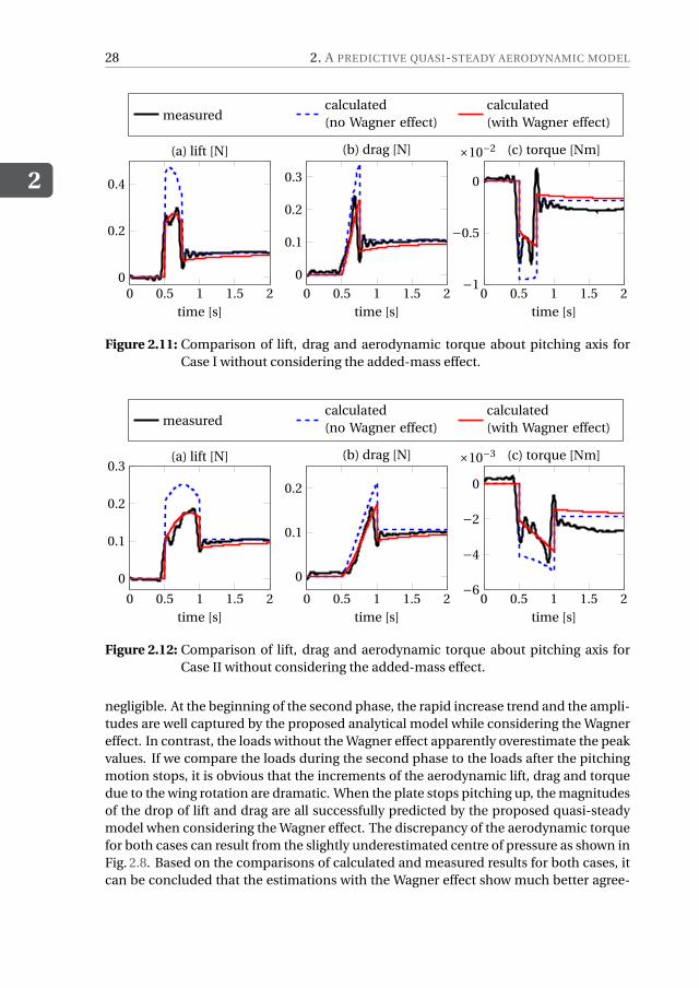
2
28 2. A PREDICTIVE QUASI-STEADY AERODYNAMIC MODEL
0 0.5 1 1.5 20
0.2
0.4
time [s]
(a) lift [N]
0 0.5 1 1.5 20
0.1
0.2
0.3
time [s]
(b) drag [N]
0 0.5 1 1.5 2−1
−0.5
0
×10−2
time [s]
(c) torque [Nm]
measuredcalculated(no Wagner effect)
calculated(with Wagner effect)
Figure 2.11: Comparison of lift, drag and aerodynamic torque about pitching axis forCase I without considering the added-mass effect.
0 0.5 1 1.5 2
0
0.1
0.2
0.3
time [s]
(a) lift [N]
0 0.5 1 1.5 2
0
0.1
0.2
time [s]
(b) drag [N]
0 0.5 1 1.5 2−6
−4
−2
0
×10−3
time [s]
(c) torque [Nm]
measuredcalculated(no Wagner effect)
calculated(with Wagner effect)
Figure 2.12: Comparison of lift, drag and aerodynamic torque about pitching axis forCase II without considering the added-mass effect.
negligible. At the beginning of the second phase, the rapid increase trend and the ampli-tudes are well captured by the proposed analytical model while considering the Wagnereffect. In contrast, the loads without the Wagner effect apparently overestimate the peakvalues. If we compare the loads during the second phase to the loads after the pitchingmotion stops, it is obvious that the increments of the aerodynamic lift, drag and torquedue to the wing rotation are dramatic. When the plate stops pitching up, the magnitudesof the drop of lift and drag are all successfully predicted by the proposed quasi-steadymodel when considering the Wagner effect. The discrepancy of the aerodynamic torquefor both cases can result from the slightly underestimated centre of pressure as shown inFig. 2.8. Based on the comparisons of calculated and measured results for both cases, itcan be concluded that the estimations with the Wagner effect show much better agree-
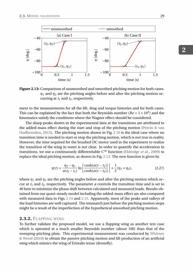
2.3. MODEL VALIDATION
2
29
0 0.5 1 1.5−100
−80
−60
−40
(t1,η1)
(t2,η2)
time [s]
η[d
eg.]
(a) Case I
0 0.5 1 1.5−100
−80
−60
−40
(t1,η1)
(t2,η2)
time [s]
η[d
eg.]
(b) Case II
unsmoothed smoothed
Figure 2.13: Comparison of unsmoothed and smoothed pitching motion for both cases.η1 and η2 are the pitching angles before and after the pitching motion oc-curring at t1 and t2, respectively.
ment to the measurements for all the lift, drag and torque histories and for both cases.This can be explained by the fact that both the Reynolds number (Re = 1×10⁴) and thekinematics satisfy the conditions where the Wagner effect should be considered.
The sharp peaks shown in the experimental data at the transitions are attributed tothe added-mass effect during the start and stop of the pitching motion (Percin & vanOudheusden, 2015). The pitching motion shown in Fig. 2.10 is the ideal case where notransition time is needed to start or stop the pitching motion, which is not true in reality.However, the time required for the brushed DC motor used in the experiment to realizethe transition of the wing in water is not clear. In order to quantify the acceleration intransitions, we use a continuously differentiable C∞ function (Eldredge et al., 2009) toreplace the ideal pitching motion, as shown in Fig. 2.13. The new function is given by
η(t ) = η2 −η1
a(t2 − t1)ln
[cosh(a(t − t1))
cosh(a(t − t2))
]+ 1
2(η1 +η2), (2.27)
where η1 and η2 are the pitching angles before and after the pitching motion which oc-cur at t1 and t2, respectively. The parameter a controls the transition time and is set to40 here to minimize the phase shift between calculated and measured loads. Results ob-tained from our quasi-steady model including the added-mass effect are also comparedwith measured data in Figs. 2.14 and 2.15. Apparently, most of the peaks and valleys ofthe load histories are well captured. The mismatch just before the pitching motion stopsmight be a result of the imperfection of the hypothetical smoothed pitching motion.
2.3.2. FLAPPING WING
To further validate the proposed model, we use a flapping wing as another test casewhich is operated at a much smaller Reynolds number (about 100) than that of thesweeping-pitching plate. This experimental measurement was conducted by Whitney& Wood (2010) to obtain the passive pitching motion and lift production of an artificialwing which mimics the wing of Eristalis tenax (dronefly).
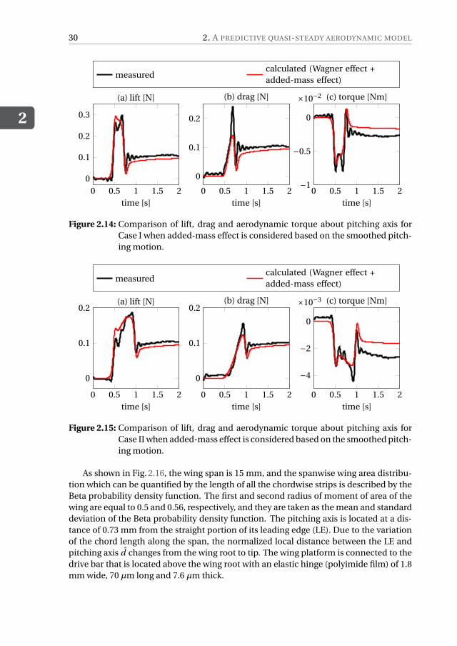
2
30 2. A PREDICTIVE QUASI-STEADY AERODYNAMIC MODEL
0 0.5 1 1.5 20
0.1
0.2
0.3
time [s]
(a) lift [N]
0 0.5 1 1.5 2
0
0.1
0.2
time [s]
(b) drag [N]
0 0.5 1 1.5 2−1
−0.5
0
×10−2
time [s]
(c) torque [Nm]
measuredcalculated (Wagner effect +added-mass effect)
Figure 2.14: Comparison of lift, drag and aerodynamic torque about pitching axis forCase I when added-mass effect is considered based on the smoothed pitch-ing motion.
0 0.5 1 1.5 2
0
0.1
0.2
time [s]
(a) lift [N]
0 0.5 1 1.5 2
0
0.1
0.2
time [s]
(b) drag [N]
0 0.5 1 1.5 2
−4
−2
0
×10−3
time [s]
(c) torque [Nm]
measuredcalculated (Wagner effect +added-mass effect)
Figure 2.15: Comparison of lift, drag and aerodynamic torque about pitching axis forCase II when added-mass effect is considered based on the smoothed pitch-ing motion.
As shown in Fig. 2.16, the wing span is 15 mm, and the spanwise wing area distribu-tion which can be quantified by the length of all the chordwise strips is described by theBeta probability density function. The first and second radius of moment of area of thewing are equal to 0.5 and 0.56, respectively, and they are taken as the mean and standarddeviation of the Beta probability density function. The pitching axis is located at a dis-tance of 0.73 mm from the straight portion of its leading edge (LE). Due to the variationof the chord length along the span, the normalized local distance between the LE andpitching axis d changes from the wing root to tip. The wing platform is connected to thedrive bar that is located above the wing root with an elastic hinge (polyimide film) of 1.8mm wide, 70 µm long and 7.6 µm thick.
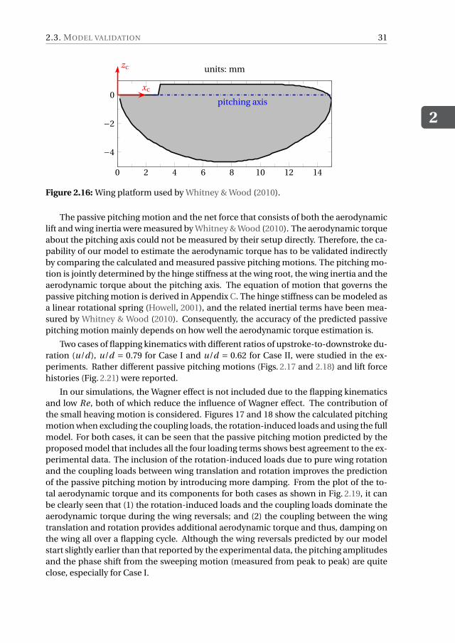
2.3. MODEL VALIDATION
2
31
0 2 4 6 8 10 12 14
−4
−2
0pitching axis
units: mm
xc
zc
Figure 2.16: Wing platform used by Whitney & Wood (2010).
The passive pitching motion and the net force that consists of both the aerodynamiclift and wing inertia were measured by Whitney & Wood (2010). The aerodynamic torqueabout the pitching axis could not be measured by their setup directly. Therefore, the ca-pability of our model to estimate the aerodynamic torque has to be validated indirectlyby comparing the calculated and measured passive pitching motions. The pitching mo-tion is jointly determined by the hinge stiffness at the wing root, the wing inertia and theaerodynamic torque about the pitching axis. The equation of motion that governs thepassive pitching motion is derived in Appendix C. The hinge stiffness can be modeled asa linear rotational spring (Howell, 2001), and the related inertial terms have been mea-sured by Whitney & Wood (2010). Consequently, the accuracy of the predicted passivepitching motion mainly depends on how well the aerodynamic torque estimation is.
Two cases of flapping kinematics with different ratios of upstroke-to-downstroke du-ration (u/d), u/d = 0.79 for Case I and u/d = 0.62 for Case II, were studied in the ex-periments. Rather different passive pitching motions (Figs. 2.17 and 2.18) and lift forcehistories (Fig. 2.21) were reported.
In our simulations, the Wagner effect is not included due to the flapping kinematicsand low Re, both of which reduce the influence of Wagner effect. The contribution ofthe small heaving motion is considered. Figures 17 and 18 show the calculated pitchingmotion when excluding the coupling loads, the rotation-induced loads and using the fullmodel. For both cases, it can be seen that the passive pitching motion predicted by theproposed model that includes all the four loading terms shows best agreement to the ex-perimental data. The inclusion of the rotation-induced loads due to pure wing rotationand the coupling loads between wing translation and rotation improves the predictionof the passive pitching motion by introducing more damping. From the plot of the to-tal aerodynamic torque and its components for both cases as shown in Fig. 2.19, it canbe clearly seen that (1) the rotation-induced loads and the coupling loads dominate theaerodynamic torque during the wing reversals; and (2) the coupling between the wingtranslation and rotation provides additional aerodynamic torque and thus, damping onthe wing all over a flapping cycle. Although the wing reversals predicted by our modelstart slightly earlier than that reported by the experimental data, the pitching amplitudesand the phase shift from the sweeping motion (measured from peak to peak) are quiteclose, especially for Case I.
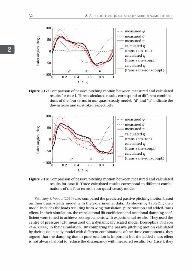
2
32 2. A PREDICTIVE QUASI-STEADY AERODYNAMIC MODEL
0 0.2 0.4 0.6 0.8 1−100
−50
0
50
100
d u d
t/T [-]
Eu
ler
angl
es[d
eg.]
measured φ
measured θmeasured η
calculated η
(trans.+am+rot.)calculated η
(trans.+am+coupl.)calculated η
(trans.+am+rot.+coupl.)
Figure 2.17: Comparison of passive pitching motion between measured and calculatedresults for case I. Three calculated results correspond to different combina-tions of the four terms in our quasi-steady model. “d" and “u" indicate thedownstroke and upstroke, respectively.
0 0.2 0.4 0.6 0.8 1−100
−50
0
50
100
d u d
t/T [-]
Eu
ler
angl
es[d
eg.]
measured φ
measured θmeasured η
calculated η
(trans.+am+rot.)calculated η
(trans.+am+coupl.)calculated η
(trans.+am+rot.+coupl.)
Figure 2.18: Comparison of passive pitching motion between measured and calculatedresults for case II. Three calculated results correspond to different combi-nations of the four terms in our quasi-steady model.
Whitney & Wood (2010) also compared the predicted passive pitching motion basedon their quasi-steady model with the experimental data. As shown by Table 2.1, theirmodel includes the loads resulting from wing translation, pure rotation and added-masseffect. In their simulation, the translational lift coefficient and rotational damping coef-ficient were tuned to achieve best agreements with experimental results. They used thecentre of pressure (CP) measured on a dynamically scaled model Drosophila Dicksonet al. (2006) in their simulation. By comparing the passive pitching motion calculatedby their quasi-steady model with different combinations of the three components, theyargued that the damping due to pure rotation is important but the added-mass effectis not always helpful to reduce the discrepancy with measured results. For Case I, they
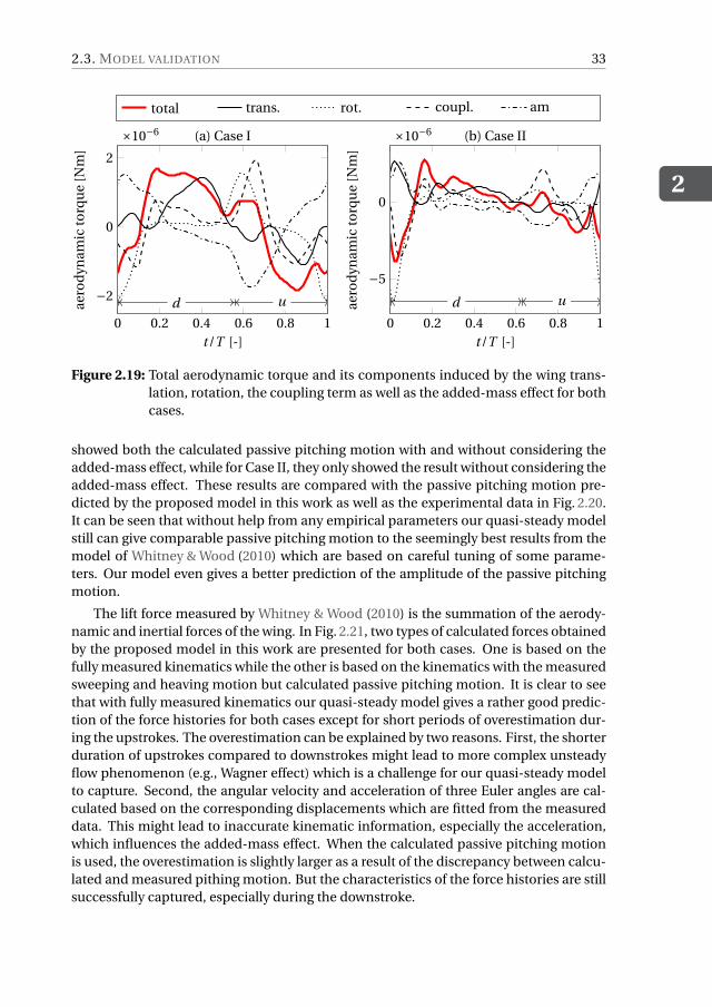
2.3. MODEL VALIDATION
2
33
0 0.2 0.4 0.6 0.8 1
−2
0
2
×10−6
d u
t/T [-]
aero
dyn
amic
torq
ue
[Nm
]
(a) Case I
0 0.2 0.4 0.6 0.8 1
−5
0
×10−6
d u
t/T [-]ae
rod
ynam
icto
rqu
e[N
m]
(b) Case II
total trans. rot. coupl. am
Figure 2.19: Total aerodynamic torque and its components induced by the wing trans-lation, rotation, the coupling term as well as the added-mass effect for bothcases.
showed both the calculated passive pitching motion with and without considering theadded-mass effect, while for Case II, they only showed the result without considering theadded-mass effect. These results are compared with the passive pitching motion pre-dicted by the proposed model in this work as well as the experimental data in Fig. 2.20.It can be seen that without help from any empirical parameters our quasi-steady modelstill can give comparable passive pitching motion to the seemingly best results from themodel of Whitney & Wood (2010) which are based on careful tuning of some parame-ters. Our model even gives a better prediction of the amplitude of the passive pitchingmotion.
The lift force measured by Whitney & Wood (2010) is the summation of the aerody-namic and inertial forces of the wing. In Fig. 2.21, two types of calculated forces obtainedby the proposed model in this work are presented for both cases. One is based on thefully measured kinematics while the other is based on the kinematics with the measuredsweeping and heaving motion but calculated passive pitching motion. It is clear to seethat with fully measured kinematics our quasi-steady model gives a rather good predic-tion of the force histories for both cases except for short periods of overestimation dur-ing the upstrokes. The overestimation can be explained by two reasons. First, the shorterduration of upstrokes compared to downstrokes might lead to more complex unsteadyflow phenomenon (e.g., Wagner effect) which is a challenge for our quasi-steady modelto capture. Second, the angular velocity and acceleration of three Euler angles are cal-culated based on the corresponding displacements which are fitted from the measureddata. This might lead to inaccurate kinematic information, especially the acceleration,which influences the added-mass effect. When the calculated passive pitching motionis used, the overestimation is slightly larger as a result of the discrepancy between calcu-lated and measured pithing motion. But the characteristics of the force histories are stillsuccessfully captured, especially during the downstroke.
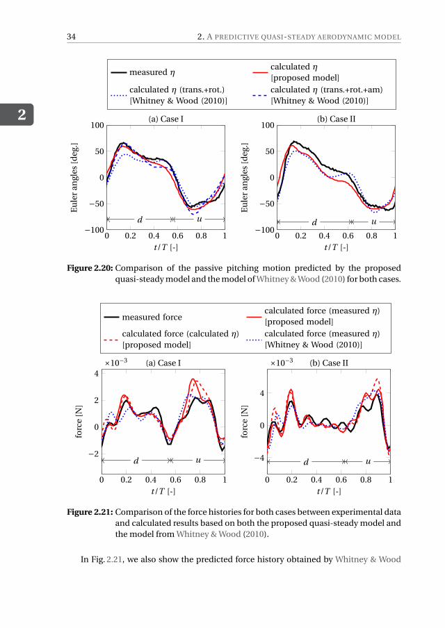
2
34 2. A PREDICTIVE QUASI-STEADY AERODYNAMIC MODEL
0 0.2 0.4 0.6 0.8 1−100
−50
0
50
100
d u d
t/T [-]
Eu
ler
angl
es[d
eg.]
(a) Case I
measured ηcalculated η
[proposed model]calculated η (trans.+rot.)[Whitney & Wood (2010)]
calculated η (trans.+rot.+am)[Whitney & Wood (2010)]
0 0.2 0.4 0.6 0.8 1−100
−50
0
50
100
d u d
t/T [-]E
ule
ran
gles
[deg
.]
(b) Case II
Figure 2.20: Comparison of the passive pitching motion predicted by the proposedquasi-steady model and the model of Whitney & Wood (2010) for both cases.
0 0.2 0.4 0.6 0.8 1
−2
0
2
4×10⁻³
d u d
t/T [-]
forc
e[N
]
(a) Case I
measured forcecalculated force (measured η)[proposed model]
calculated force (calculated η)[proposed model]
calculated force (measured η)[Whitney & Wood (2010)]
0 0.2 0.4 0.6 0.8 1
−4
0
4
×10−3
d u d
t/T [-]
forc
e[N
]
(b) Case II
Figure 2.21: Comparison of the force histories for both cases between experimental dataand calculated results based on both the proposed quasi-steady model andthe model from Whitney & Wood (2010).
In Fig. 2.21, we also show the predicted force history obtained by Whitney & Wood
2.4. CONCLUSIONS
2
35
(2010). In their simulation, the pure rotation effect is ignored during the force calcula-tion although included in the aerodynamic torque estimation for calculating the passivepitching motion. Even though the careful selection of different terms and tuning of em-pirical parameters do improve the agreement of lift prediction with measured data, theirmodel is less predictive for arbitrary flapping wings compared to our quasi-steady modelwhich does not rely on any empirical data.
The measured average lift forces are 71.6 mg for Case I and 71.2 mg for Case II, re-spectively. With the proposed quasi-steady model, the average lift based on the fullymeasured kinematics is 90.9 mg and 81.6 mg for two cases, respectively. Due to the in-crease of discrepancy between measured and calculated pitching motion, the averagelift obtained based on the calculated pitching motion is 89.0 mg for Case I and 94.4 mgfor Case II. In addition to the error of the predicted passive pitching motion, this overes-timated average lift force might be attributed to the fact that the lift is very sensitive tothe wing dimensions. For example, if we decrease the wing span by 1 mm while keep-ing the aspect ratio, the calculated average lift forces based on measured kinematics arereduced to 75.1 and 66.7 mg for the two cases.
Without using any empirical parameters or selectively choosing different terms, ourquasi-steady model is still able to give good predictions to the passive pitching motion.Compared to the results obtained by the quasi-steady model proposed by Whitney &Wood (2010), the proposed model can give a comparable or slightly better prediction ofthe passive pitching motion. This implies that our model is more predictive for evaluat-ing the aerodynamic performance of flapping wings in passive pitching motion. Admit-tedly, limited by the inherent drawbacks of the quasi-steady assumption, the unsteadyeffects, such as wake capture effect, the Wagner effect and the spatial movement of theLEV on the wing surface, can not be reflected. This might be another reason of the dis-crepancy of the passive pitching motion and force history between calculated and ex-perimental results.
2.4. CONCLUSIONSFor wings performing translational and rotational motion simultaneously, particularlyfor flapping wings, we proposed a predictive quasi-steady aerodynamic model. Thismodel is capable of predicting both the aerodynamic force and torque, and it also pro-vides better solutions to three issues which have not been addressed completely by ex-isting quasi-steady models. First is the inconsistency of compositions of existing quasi-steady models, which is eliminated by comprehensively including contributions fromwing translation, rotation, their coupling and the added-mass effect in the proposedmodel. Second is the overall contribution of the wing rotation to the total aerodynamicloads and the corresponding centre of pressure, both of which are required for the esti-mation of aerodynamic torque. We use two components, including the rotation-inducedloads due to the pure wing rotation and the loads due to the coupling between wing ro-tation and translation, to collaboratively represent the overall contribution of the wingrotation. A new formula for the coupling load has been derived based on the conditionthat the plate uniformly rotates around its pitching axis in an incoming flow. This con-dition should be applied as a result of the “quasi-steady” assumption. However, the for-mula used in most existing quasi-steady models assumes that the plate oscillates around

2
36 2. A PREDICTIVE QUASI-STEADY AERODYNAMIC MODEL
its equilibrium position in a harmonic way. The importance of both components to thequasi-steady model has been shown by the fact that the damping torque excluding thecontribution from either of them is far from sufficient to maintain the expected passivepitching motion. The proposed model shows excellent prediction of the centre of pres-sure of a dynamically scaled hawkmoth wing conducting translational and rotationalmotion simultaneously at different angles of attack. Third is that most existing quasi-steady models depend on empirical parameters. In contrast, the proposed model doesnot rely on any empirical data while it still shows a comparable accuracy on estimatingthe aerodynamic force, torque and the passive pitching motion as shown by the com-parisons with experimental data of two test cases. This implies that the proposed modelis more predictive compared to existing quasi-steady models. Therefore, the proposedquasi-steady model can be applied to the design and optimization of flapping wings.
3OPTIMAL PITCHING AXIS LOCATION
OF FLAPPING WINGS FOR EFFICIENT
HOVERING FLIGHT
Flapping wings can pitch passively about their pitching axes due to their flexibility, iner-tia, and aerodynamic loads. A shift in the pitching axis location can dynamically alter theaerodynamic loads, which in turn changes the passive pitching motion and the flight effi-ciency. Therefore, it is of great interest to investigate the optimal pitching axis for flappingwings to maximize the power efficiency during hovering flight.
In this chapter, flapping wings are modeled as rigid plates with non-uniform mass distri-bution. The wing flexibility is represented by a linearly torsional spring at the wing root.The quasi-steady aerodynamic model introduced in Chapter 2 is used to evaluate the liftgenerated by such wings. Two extreme power consumption scenarios are modeled for hov-ering flight, i.e., the power consumed by a drive system with and without the capacity ofkinetic energy recovery. For wings with different shapes, the optimal pitching axis loca-tion is found such that the cycle-averaged power consumption during hovering flight isminimized. This chapter is organized as follows. Sec. 3.1 introduces the background andmotivation. The following sections start with the flapping wing modeling in Sec. 3.2 whichconsists of the wing area and mass distribution models as well as the kinematics model.In Sec. 3.3, the aerodynamic model and the power consumption model are introduced.Based on the optimization model described in Sec. 3.4, we investigate the optimal loca-tion of pitching axis for different wings and analyse its influences on the power efficiencyduring hovering flight in Sec. 3.5. Conclusions are presented in Sec. 4.5.
This chapter is based on the paper “Wang, Q., Goosen, J.F.L., Van Keulen, F., 2017. Optimal pitching axis loca-tion of flapping wings for efficient hovering flight (submitted to Bioinspiration & Biomimetics)”.
37
3
38 3. OPTIMAL PITCHING AXIS LOCATION OF FLAPPING WINGS
3.1. INTRODUCTIONThere exists a great diversity of wing morphology among insects, especially from thewing shape perspective. Compared to the wing outlines of various winged-insects, thewings of most flapping wing micro air vehicles (FWMAVs) (de Croon et al., 2009, Bolsmanet al., 2009, Keennon et al., 2012, Ma et al., 2013, Nguyen et al., 2015) have much simplershapes (e.g., quarter-ellipse, polygon). Although this simplification helps to decreasethe design complexity and fabrication difficulty, the effect of wing shape on the flappingflight performance, particularly on the energy-efficiency, can not be completely ignored.
Wing shape determines the area distribution which can be further decomposed intodistributions in the span and chord directions. Aerodynamic loads on flapping wingsroughly increase quadratically with the velocity and, thus, are sensitive to the spanwisearea distribution (SWAD). As a result, its influence on flapping wing performance hasbeen extensively studied in the past. For instance, Ansari et al. (2008) investigated theinfluence of the spanwise wing area distribution and aspect ratio on the lift generationand power efficiency using an unsteady aerodynamic model (Ansari, 2004). Recently,Shahzad et al. (2016) conducted similar investigations using a computational fluid dy-namics (CFD) method. They both showed that wings with more outboard area andhigher aspect ratio generate higher lift but also consume more power. This is becausethe lift and power scale with the square and cube of flapping velocity, respectively. Op-timal wing shapes have also been studied in literature using quasi-steady aerodynamicmodels. Typically, the total lift force is constrained in these studies. By keeping the wingaspect ratio constant, Wang et al. (2013) showed that flapping wings with more outboardarea can have better performance, i.e., higher lift generation or less power consumption.Stewart et al. (2013) found that the optimal wing shape which provides maximal thrustfor forward flight tends to push much of the planform away from the wing root. Wanget al. (2014a) investigated the optimal wing shape for energy-efficient hovering flight inpassive pitching motion while keeping the total wing area constant. A wing planformwith a low aspect ratio, similar to butterfly wings, was obtained.
In contrast, the influence of chordwise area distribution (CWAD) on flapping flightperformance has been less studied. CWAD determines the inertia and aerodynamicloads a wing needs to overcome when pitching about its pitching axis. Particularly whenthe wing pitches passively due to its flexibility and the inertial and aerodynamic loadsCWAD directly determines the passive pitching behavior, including the amplitude, thephase lag from sweeping motion, and its deviation from a harmonic motion. Passivepitching can be found for both insects (Ennos, 1989, Combes & Daniel, 2003, Bergouet al., 2007, Ishihara et al., 2009) and FWMAVs (Wood, 2008, de Croon et al., 2009, Keen-non et al., 2012, Ma et al., 2013). Particularly for FWMAVs, the passive pitching motionis preferred in order to simplify the drive mechanism. Consequently, the location of thepitching axis becomes an important design aspect for artificial wings in order to achieveenergy-efficient flight for FWMAVs.
This work aims to find the optimal pitching axis location for flapping wings with pas-sive pitching motion. Flapping wings are modeled as rigid plates with non-uniform massdistribution. The wing flexibility is represented by a linearly torsional spring at the wingroot, which is commonly used for the wing design (Whitney & Wood, 2010, Wang et al.,2014a). The predictive quasi-steady aerodynamic model presented in Chapter 2 is used
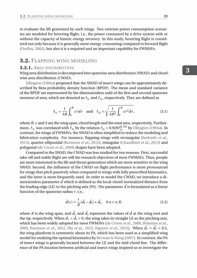
3.2. FLAPPING WING MODELING
3
39
to evaluate the lift generated by such wings. Two extreme power consumption scenar-ios are modeled for hovering flight, i.e., the power consumed by a drive system with orwithout the capacity of kinetic energy recovery. In this study, hovering flight is consid-ered not only because it is generally more energy-consuming compared to forward flight(Dudley, 2002), but also it is a required and an important capability for FWMAVs.
3.2. FLAPPING WING MODELING
3.2.1. AREA DISTRIBUTIONWing area distribution is decomposed into spanwise area distribution (SWAD) and chord-wise area distribution (CWAD).
Ellington (1984a) proposed that the SWAD of insect wings can be approximately de-scribed by Beta probability density function (BPDF). The mean and standard varianceof the BPDF are represented by the dimensionless radii of the first and second spanwisemoment of area, which are denoted as rs1 and rs2 , respectively. They are defined as
rs1 =1
SR
∫ R
0cr dr and rs2 =
√1
SR2
∫ R
0cr 2dr , (3.1)
where R, c and S are the wing span, chord length and the total area, respectively. Further-more, rs1 was correlated with rs2 by the relation rs2 = 0.929r 0.732
s2by Ellington (1984a). In
contrast, for wings of FWMAVs, the SWAD is often simplified to reduce the modeling andfabrication complexity. For instance, flapping wings with rectangular (Seshadri et al.,2013), quarter-ellipsoidal (Keennon et al., 2012), triangular (Chaudhuri et al., 2013) andpolygonal (de Croon et al., 2009) shapes have been adopted.
Compared to the SWAD, the CWAD was less studied for two reasons. First, successfultake-off and stable flight are still the research objectives of most FWMAVs. Thus, peopleare more interested in the lift and thrust generation which are more sensitive to the wingSWAD. Second, the influence of the CWAD on flight performance is more pronouncedfor wings that pitch passively when compared to wings with fully prescribed kinematics,and the latter is more frequently used. In order to model the CWAD, we introduce a di-mensionless parameter d which is defined as the local-chord-normalized distance fromthe leading edge (LE) to the pitching axis (PA). The parameter d is formulated as a linearfunction of the spanwise radius r , i.e.,
d(r ) = r
R(dt − dr)+ dr, 0 É r É R, (3.2)
where R is the wing span, and dr and dt represent the values of d at the wing root andthe tip, respectively. When dr = dt = 0, the wing takes its straight LE as the pitching axis,which has been widely adopted for most FWMAVs (de Croon et al., 2009, Bolsman et al.,2009, Keennon et al., 2012, Ma et al., 2013, Nguyen et al., 2015). When dr = dt = 0.5,the wing planform is symmetric about its PA, which has been used as a simplified wingmodel for studying the optimal kinematics by Berman & Wang (2007). In contrast, the PAof insect wings is generally located between the LE and the mid-chord line. The differ-ence of the PA location between artificial and insect wings inspired us to investigate the
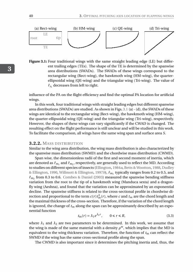
3
40 3. OPTIMAL PITCHING AXIS LOCATION OF FLAPPING WINGS
root tipLE
TE
(a) Rect-wing (b) HM-wing (c) QE-wing (d) Tri-wing
Figure 3.1: Four traditional wings with the same straight leading edge (LE) but differ-ent trailing edges (TEs). The shape of the TE is determined by the spanwisearea distributions (SWADs). The SWADs of these wings correspond to therectangular wing (Rect-wing), the hawkmoth wing (HM-wing), the quarter-ellipsoidal wing (QE-wing) and the triangular wing (Tri-wing). The value ofrs1 decreases from left to right.
influence of the PA on the flight efficiency and find the optimal PA location for artificialwings.
In this work, four traditional wings with straight leading edges but different spanwisearea distributions (SWADs) are studied. As shown in Figs. 3.1 (a) - (d), the SWADs of thesewings are identical to the rectangular wing (Rect-wing), the hawkmoth wing (HM-wing),the quarter-ellipsoidal wing (QE-wing) and the triangular wing (Tri-wing), respectively.However, the shapes of these wings can vary significantly if the CWAD is changed. Theresulting effect on the flight performance is still unclear and will be studied in this work.To facilitate the comparison, all wings have the same wing span and surface area S.
3.2.2. MASS DISTRIBUTIONSimilar to the wing area distribution, the wing mass distribution is also characterized bythe spanwise mass distribution (SWMD) and the chordwise mass distribution (CWMD).
Span wise, the dimensionless radii of the first and second moment of inertia, whichare denoted as rm1 and rm2 , respectively, are generally used to reflect the MD. Accordingto studies on different species of insects (Ellington, 1984a, Betts & Wootton, 1988, Dudley& Ellington, 1990, Willmott & Ellington, 1997b), rm1 typically ranges from 0.2 to 0.5, andrm2 from 0.3 to 0.6. Combes & Daniel (2003) measured the spanwise bending stiffnessvariation from the root to the tip of a hawkmoth wing (Manduca sexta) and a dragon-fly wing (Aeshna), and found that the variation can be approximated by an exponentialdecline. The spanwise stiffness is related to the cross-sectional profile in chordwise di-rection and proportional to the term c(r )t 3
m(r ), where c and tm are the chord length andthe maximal thickness of the cross-section. Therefore, if the variation of the chord lengthis ignored, the change of tm along the span can be approximately described by an expo-nential function
tm(r ) =λ1eλ2r , 0 É r É R, (3.3)
where λ1 and λ2 are two parameters to be determined. In this work, we assume thatthe wing is made of the same material with a density ρw, which implies that the MD isequivalent to the wing thickness variation. Therefore, the function of tm can reflect theSWMD if the wing has the same cross-sectional profile along the span.
The CWMD is also important since it determines the pitching inertia and, thus, the
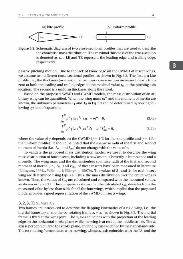
3.2. FLAPPING WING MODELING
3
41
LE TEtm tmLE TE
(a) kite profile (b) uniform profile
Figure 3.2: Schematic diagram of two cross-sectional profiles that are used to describethe chordwise mass distribution. The maximal thickness of the cross-sectionis denoted as tm. LE and TE represent the leading edge and trailing edge,respectively.
passive pitching motion. Due to the lack of knowledge on the CWMD of insect wings,we assume two different cross-sectional profiles, as shown in Fig. 3.2. The first is a kiteprofile, i.e., the thickness (or mass) of an arbitrary cross-section increases linearly fromzero at both the leading and trailing edges to the maximal value tm at the pitching axislocation. The second is a uniform thickness along the chord.
Based on the proposed SWMD and CWMD models, the mass distribution of an ar-bitrary wing can be quantified. When the wing mass mw and the moment of inertia areknown, the unknown parameters λ1 and λ2 in Eq. 3.3 can be determined by solving fol-lowing system of equations
∫ R
0ρwγλ1eλ2r cdr −mw = 0, (3.4a)
∫ R
0ρwγλ1eλ2r cr 2dr −mwr 2
m2= 0, (3.4b)
where the value of γ depends on the CWMD (γ = 1/2 for the kite profile and γ = 1 forthe uniform profile). It should be noted that the spanwise radii of the first and secondmoment of inertia (i.e., rm1 and rm2 ) do not change with the value of γ.
To validate the proposed mass distribution model, we use it to describe the wingmass distribution of four insects, including a hawkmoth, a hoverfly, a bumblebee and adronefly. The wing mass and the dimensionless spanwise radii of the first and secondmoment of inertia (i.e., rm1 and rm2 ) of these insects have been measured in literature(Ellington, 1984a, Willmott & Ellington, 1997b). The values of λ1 and λ2 for each insectwing are determined using Eqs. 3.4. Thus, the mass distribution over the entire wing isknown. Then, the values of rm1 are calculated and compared with the measured values,as shown in Table 3.1. The comparison shows that the calculated rm1 deviates from themeasured value by less than 6.9% for all the four wings, which implies that the proposedmodel provides a good representation of the SWMD of insects wings.
3.2.3. KINEMATICSTwo frames are introduced to describe the flapping kinematics of a rigid wing, i.e., theinertial frame xi yizi and the co-rotating frame xc yczc, as shown in Fig. 3.3. The inertialframe is fixed at the wing joint. The xi axis coincides with the projection of the leadingedge on the horizontal stroke plane while the wing is at rest at the middle stroke. The zi
axis is perpendicular to the stroke plane, and the yi axis is defined by the right-hand-rule.The co-rotating frame rotates with the wing, whose xc axis coincides with the PA, and the
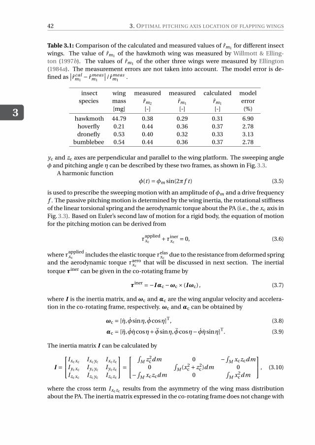
3
42 3. OPTIMAL PITCHING AXIS LOCATION OF FLAPPING WINGS
Table 3.1: Comparison of the calculated and measured values of rm1 for different insectwings. The value of rm1 of the hawkmoth wing was measured by Willmott & Elling-ton (1997b). The values of rm1 of the other three wings were measured by Ellington(1984a). The measurement errors are not taken into account. The model error is de-fined as
∣∣r calm1
− r measm1
∣∣/r measm1
.
insect wing measured measured calculated modelspecies mass rm2 rm1 rm1 error
[mg] [-] [-] [-] (%)
hawkmoth 44.79 0.38 0.29 0.31 6.90hoverfly 0.21 0.44 0.36 0.37 2.78dronefly 0.53 0.40 0.32 0.33 3.13
bumblebee 0.54 0.44 0.36 0.37 2.78
yc and zc axes are perpendicular and parallel to the wing platform. The sweeping angleφ and pitching angle η can be described by these two frames, as shown in Fig. 3.3.
A harmonic functionφ(t ) =φm sin(2π f t ) (3.5)
is used to prescribe the sweeping motion with an amplitude ofφm and a drive frequencyf . The passive pitching motion is determined by the wing inertia, the rotational stiffnessof the linear torsional spring and the aerodynamic torque about the PA (i.e., the xc axis inFig. 3.3). Based on Euler’s second law of motion for a rigid body, the equation of motionfor the pitching motion can be derived from
τappliedxc
+τinerxc
= 0, (3.6)
where τappliedxc
includes the elastic torque τelasxc
due to the resistance from deformed springand the aerodynamic torque τaero
xcthat will be discussed in next section. The inertial
torque τiner can be given in the co-rotating frame by
τiner =−Iαc −ωc × (Iωc) , (3.7)
where I is the inertia matrix, and ωc and αc are the wing angular velocity and accelera-tion in the co-rotating frame, respectively. ωc andαc can be obtained by
ωc = [η, φsinη, φcosη]T, (3.8)
αc = [η, φηcosη+ φsinη, φcosη− φηsinη]T. (3.9)
The inertia matrix I can be calculated by
I =
Ixcxc Ixc yc Ixczc
Iycxc Iyc yc Iyczc
Izcxc Izc yc Izczc
=
∫M z2
c dm 0 −∫M xczcdm
0∫
M (x2c + z2
c )dm 0−∫
M xczcdm 0∫
M x2c dm
, (3.10)
where the cross term Ixczc results from the asymmetry of the wing mass distributionabout the PA. The inertia matrix expressed in the co-rotating frame does not change with
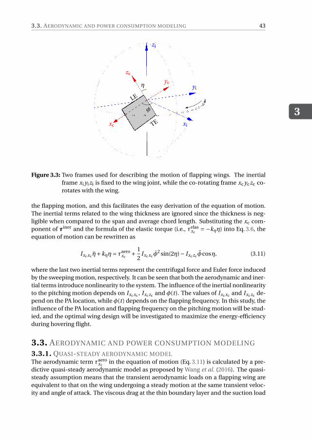
3.3. AERODYNAMIC AND POWER CONSUMPTION MODELING
3
43
xc
yc
zc
xi
yi
zi
LE
TE
φ
η
Figure 3.3: Two frames used for describing the motion of flapping wings. The inertialframe xi yizi is fixed to the wing joint, while the co-rotating frame xc yczc co-rotates with the wing.
the flapping motion, and this facilitates the easy derivation of the equation of motion.The inertial terms related to the wing thickness are ignored since the thickness is neg-ligible when compared to the span and average chord length. Substituting the xc com-ponent of τiner and the formula of the elastic torque (i.e., τelas
xc= −kηη) into Eq. 3.6, the
equation of motion can be rewritten as
Ixcxc η+kηη= τaeroxc
+ 1
2Ixcxc φ
2 sin(2η)− Ixczc φcosη, (3.11)
where the last two inertial terms represent the centrifugal force and Euler force inducedby the sweeping motion, respectively. It can be seen that both the aerodynamic and iner-tial terms introduce nonlinearity to the system. The influence of the inertial nonlinearityto the pitching motion depends on Ixcxc , Ixczc and φ(t ). The values of Ixcxc and Ixczc de-pend on the PA location, whileφ(t ) depends on the flapping frequency. In this study, theinfluence of the PA location and flapping frequency on the pitching motion will be stud-ied, and the optimal wing design will be investigated to maximize the energy-efficiencyduring hovering flight.
3.3. AERODYNAMIC AND POWER CONSUMPTION MODELING
3.3.1. QUASI-STEADY AERODYNAMIC MODELThe aerodynamic term τaero
xcin the equation of motion (Eq. 3.11) is calculated by a pre-
dictive quasi-steady aerodynamic model as proposed by Wang et al. (2016). The quasi-steady assumption means that the transient aerodynamic loads on a flapping wing areequivalent to that on the wing undergoing a steady motion at the same transient veloc-ity and angle of attack. The viscous drag at the thin boundary layer and the suction load
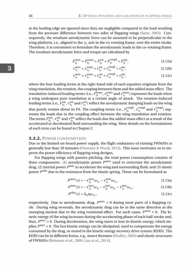
3
44 3. OPTIMAL PITCHING AXIS LOCATION OF FLAPPING WINGS
at the leading edge are ignored since they are negligible compared to the load resultingfrom the pressure difference between two sides of flapping wings (Sane, 2003). Con-sequently, the resultant aerodynamic force can be assumed to be perpendicular to thewing platform, i.e., aligned to the yc axis in the co-rotating frame, over the entire stroke.Therefore, it is convenient to formulate the aerodynamic loads in the co-rotating frame.The resultant aerodynamic force and torque are calculated by
F aeroyc
= F transyc
+F rotyc
+F couplyc
+F amyc
, (3.12a)
τaeroxc
= τtransxc
+τrotxc
+τcouplxc
+τamxc
, (3.12b)
τaerozc
= τtranszc
+τrotzc
+τcouplzc
+τamzc
, (3.12c)
where the four loading terms at the right-hand side of each equation originate from thewing translation, the rotation, the couping between them and the added mass effect. Thetranslation-induced loading terms (i.e., F trans
yc, τtrans
xcand τtrans
zc) represent the loads when
a wing undergoes pure translation at a certain angle of attack. The rotation-inducedloading terms (i.e., F rot
yc, τrot
xcand τrot
zc) reflect the aerodynamic damping loads on the wing
that purely rotates about its PA. The coupling terms (i.e., F couplyc
, τcouplxc
and τcouplzc
) rep-resent the loads due to the coupling effect between the wing translation and rotation.The terms F am
yc, τam
xcand τam
zcreflect the loads due the added-mass effect as a result of the
accelerated or decelerated fluid surrounding the wing. More details on the formulationsof each term can be found in Chapter 2.
3.3.2. POWER CONSUMPTIONDue to the limited on-board power supply, the flight endurance of existing FWMAVs isgenerally less than 20 minutes (Floreano & Wood, 2015). This issue motivates us to im-prove the power efficiency of flapping wing designs.
For flapping wings with passive pitching, the total power consumption consists ofthree components: (1) aerodynamic power P aero used to overcome the aerodynamicdrag, (2) inertial power P iner to accelerate the wing and surrounding fluid, and (3) elasticpower P elas due to the resistance from the elastic spring. These can be formulated as
P aero(t ) =−τaeroxc
ωxc −τaerozc
ωzc , (3.13a)
P iner(t ) =−τinerxc
ωxc −τineryc
ωyc −τinerzc
ωzc , (3.13b)
P elas(t ) = kηηωxc , (3.13c)
respectively. Due to aerodynamic drag, P aero > 0 during most parts of a flapping cy-cle. During wing reversals, the aerodynamic drag can be in the same direction as thesweeping motion due to the wing rotational effect. For such cases, P aero < 0. The ki-netic energy of the wing increases during the accelerating phase of each half-stroke and,thus, P iner > 0. During deceleration, the wing starts to lose its kinetic energy, which im-plies P iner < 0. The lost kinetic energy can be dissipated, used to compensate the energyconsumed by the drag, or stored in the kinetic energy recovery drive system (KERS). TheKERS can be in different forms, e.g., insect thoraxes (Dudley, 2002) and elastic structuresof FWMAVs (Bolsman et al., 2009, Lau et al., 2014).
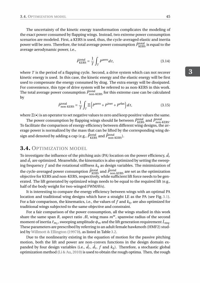
3.4. OPTIMIZATION MODEL
3
45
The uncertainty of the kinetic energy transformation complicates the modeling ofthe exact power consumed by flapping wings. Instead, two extreme power consumptionscenarios are modeled. First, a KERS is used, thus, the cycle-averaged elastic and inertiapower will be zero. Therefore, the total average power consumption P total
KERS is equal to theaverage aerodynamic power, i.e.,
P totalKERS =
1
T
∫
TP aerod t , (3.14)
where T is the period of a flapping cycle. Second, a drive system which can not recoverkinetic energy is used. In this case, the kinetic energy and the elastic energy will be firstused to compensate the energy consumed by drag. The extra energy will be dissipated.For convenience, this type of drive system will be referred to as non-KERS in this work.The total average power consumption P total
non-KERS for this extreme case can be calculatedby
P totalnon-KERS =
1
T
∫
TΞ
(P aero +P iner +P elas
)d t , (3.15)
whereΞ(•) is an operator to set negative values to zero and keep positive values the same.The power consumption by flapping wings should lie between P total
KERS and P totalnon-KERS.
To facilitate the comparison of energy-efficiency between different wing designs, the av-erage power is normalized by the mass that can be lifted by the corresponding wing de-
sign and denoted by adding a cap (e.g., ˆP totalKERS and ˆP total
non-KERS).
3.4. OPTIMIZATION MODEL
To investigate the influence of the pitching axis (PA) location on the power efficiency, dr
and dt are optimized. Meanwhile, the kinematics is also optimized by setting the sweep-ing frequency f and the rotational stiffness kη as design variables. The minimization of
the cycle-averaged power consumption ˆP totalKERS and ˆP total
non-KERS are set as the optimizationobjective for KERS and non-KERS, respectively, while sufficient lift force needs to be gen-erated. The lift generated by optimized wings needs to be equal to the required lift (e.g.,half of the body weight for two-winged FWMAVs).
It is interesting to compare the energy efficiency between wings with an optimal PAlocation and traditional wing designs which have a straight LE as the PA (see Fig. 3.1).For a fair comparison, the kinematics, i.e., the values of f and kη, are also optimized fortraditional wings subjected to the same objective and constraint.
For a fair comparison of the power consumption, all the wings studied in this workshare the same span R, aspect ratioA, wing mass mw, spanwise radius of the secondmoment of inertia rm2 , sweeping amplitudeφm and the lift generation requirement Lreq.These parameters are prescribed by referring to an adult female hawkmoth (HMF2) stud-ied by Willmott & Ellington (1997b), as listed in Table 3.2.
Due to the nonlinearity existing in the equation of motion for the passive pitchingmotion, both the lift and power are non-convex functions in the design domain ex-panded by four design variables (i.e., dr , dt , f and kη). Therefore, a stochastic globaloptimization method (Li & Au, 2010) is used to obtain the rough optima. Then, the rough
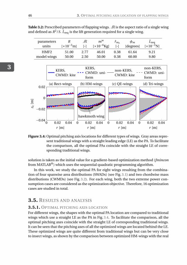
3
46 3. OPTIMAL PITCHING AXIS LOCATION OF FLAPPING WINGS
Table 3.2: Prescribed parameters of flapping wings.A is the aspect ratio of a single wingand defined as R2/S. Lreq is the lift generation required for a single wing.
parameters R A mw rm2 φm Lreq
units [×10−3m] [-] [×10−6Kg] [-] [degrees] [×10−3N]
HMF2 51.00 2.77 46.01 0.38 61.64 9.21model wings 50.00 2.50 50.00 0.38 60.00 9.80
0 0.02 0.04−0.04
−0.02
0
0.02
r [m]
z c[m
]
(a) Rect-wings
0 0.02 0.04
hawkmoth wing
r [m]
(b) HM-wings
0 0.02 0.04r [m]
(c) QE-wings
0 0.02 0.04r [m]
(d) Tri-wings
KERS,CWMD: kite
KERS,CWMD: uni-form
non-KERS,CWMD: kite
non-KERS,CWMD: uni-form
Figure 3.4: Optimal pitching axis locations for different types of wings. Gray areas repre-sent traditional wings with a straight leading edge (LE) as the PA. To facilitatethe comparison, all the optimal PAs coincide with the straight LE of corre-sponding traditional wings.
solution is taken as the initial value for a gradient-based optimization method (fminconfrom MATLAB®) which uses the sequential quadratic programming algorithm.
In this work, we study the optimal PA for eight wings resulting from the combina-tion of four spanwise area distributions (SWADs) (see Fig. 3.1) and two chordwise massdistributions (CWMDs) (see Fig. 3.2). For each wing, both the two extreme power con-sumption cases are considered as the optimization objective. Therefore, 16 optimizationcases are studied in total.
3.5. RESULTS AND ANALYSIS
3.5.1. OPTIMAL PITCHING AXIS LOCATION
For different wings, the shapes with the optimal PA location are compared to traditionalwings which use a straight LE as the PA in Fig. 3.4. To facilitate the comparison, all theoptimal pitching axes coincide with the straight LE of corresponding traditional wings.It can be seen that the pitching axes of all the optimized wings are located behind the LE.These optimized wings are quite different from traditional wings but can be very closeto insect wings, as shown by the comparison between optimized HM-wings with the real
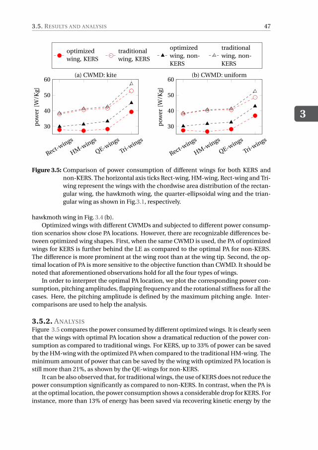
3.5. RESULTS AND ANALYSIS
3
47
Rect-wings
HM-wings
QE-wings
Tri-wings
30
40
50
60
pow
er[W
/Kg]
(a) CWMD: kite
Rect-wings
HM-wings
QE-wings
Tri-wings
30
40
50
60
pow
er[W
/Kg]
(b) CWMD: uniform
optimizedwing, KERS
traditionalwing, KERS
optimizedwing, non-KERS
traditionalwing, non-KERS
Figure 3.5: Comparison of power consumption of different wings for both KERS andnon-KERS. The horizontal axis ticks Rect-wing, HM-wing, Rect-wing and Tri-wing represent the wings with the chordwise area distribution of the rectan-gular wing, the hawkmoth wing, the quarter-ellipsoidal wing and the trian-gular wing as shown in Fig.3.1, respectively.
hawkmoth wing in Fig. 3.4 (b).Optimized wings with different CWMDs and subjected to different power consump-
tion scenarios show close PA locations. However, there are recognizable differences be-tween optimized wing shapes. First, when the same CWMD is used, the PA of optimizedwings for KERS is further behind the LE as compared to the optimal PA for non-KERS.The difference is more prominent at the wing root than at the wing tip. Second, the op-timal location of PA is more sensitive to the objective function than CWMD. It should benoted that aforementioned observations hold for all the four types of wings.
In order to interpret the optimal PA location, we plot the corresponding power con-sumption, pitching amplitudes, flapping frequency and the rotational stiffness for all thecases. Here, the pitching amplitude is defined by the maximum pitching angle. Inter-comparisons are used to help the analysis.
3.5.2. ANALYSISFigure 3.5 compares the power consumed by different optimized wings. It is clearly seenthat the wings with optimal PA location show a dramatical reduction of the power con-sumption as compared to traditional wings. For KERS, up to 33% of power can be savedby the HM-wing with the optimized PA when compared to the traditional HM-wing. Theminimum amount of power that can be saved by the wing with optimized PA location isstill more than 21%, as shown by the QE-wings for non-KERS.
It can be also observed that, for traditional wings, the use of KERS does not reduce thepower consumption significantly as compared to non-KERS. In contrast, when the PA isat the optimal location, the power consumption shows a considerable drop for KERS. Forinstance, more than 13% of energy has been saved via recovering kinetic energy by the
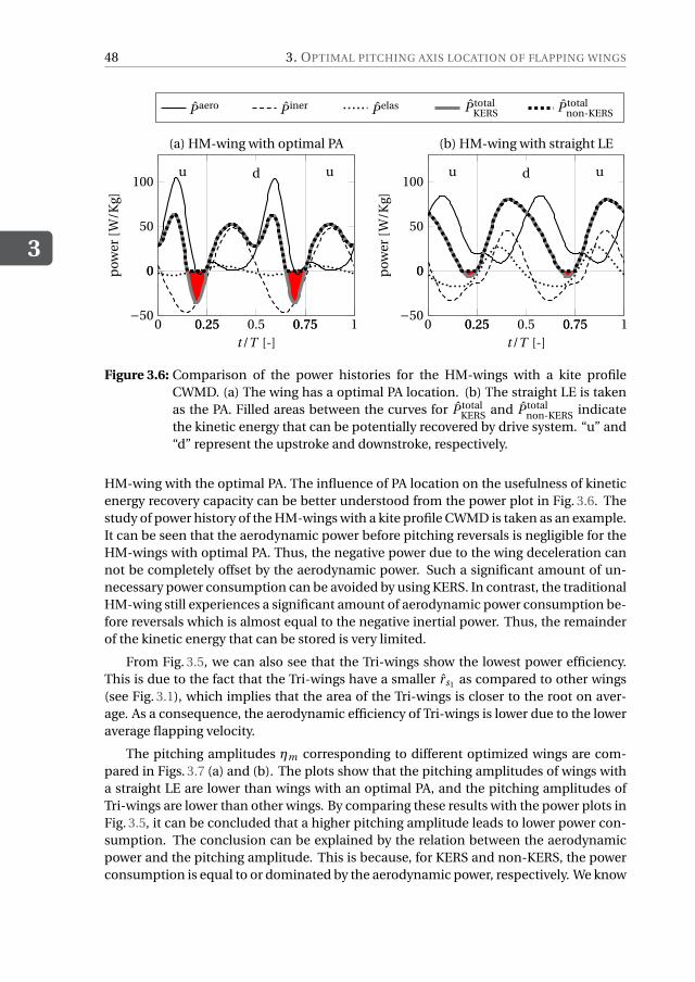
3
48 3. OPTIMAL PITCHING AXIS LOCATION OF FLAPPING WINGS
0 0.25 0.5 0.75 1−50
0
50
100
0.25 0.75
0
u d u
t/T [-]
pow
er[W
/Kg]
(a) HM-wing with optimal PA
0 0.25 0.5 0.75 1−50
0
50
100
0.25 0.75
0
u d u
t/T [-]
pow
er[W
/Kg]
(b) HM-wing with straight LE
P aero P iner P elas P totalKERS P total
non-KERS
Figure 3.6: Comparison of the power histories for the HM-wings with a kite profileCWMD. (a) The wing has a optimal PA location. (b) The straight LE is takenas the PA. Filled areas between the curves for P total
KERS and P totalnon-KERS indicate
the kinetic energy that can be potentially recovered by drive system. “u” and“d” represent the upstroke and downstroke, respectively.
HM-wing with the optimal PA. The influence of PA location on the usefulness of kineticenergy recovery capacity can be better understood from the power plot in Fig. 3.6. Thestudy of power history of the HM-wings with a kite profile CWMD is taken as an example.It can be seen that the aerodynamic power before pitching reversals is negligible for theHM-wings with optimal PA. Thus, the negative power due to the wing deceleration cannot be completely offset by the aerodynamic power. Such a significant amount of un-necessary power consumption can be avoided by using KERS. In contrast, the traditionalHM-wing still experiences a significant amount of aerodynamic power consumption be-fore reversals which is almost equal to the negative inertial power. Thus, the remainderof the kinetic energy that can be stored is very limited.
From Fig. 3.5, we can also see that the Tri-wings show the lowest power efficiency.This is due to the fact that the Tri-wings have a smaller rs1 as compared to other wings(see Fig. 3.1), which implies that the area of the Tri-wings is closer to the root on aver-age. As a consequence, the aerodynamic efficiency of Tri-wings is lower due to the loweraverage flapping velocity.
The pitching amplitudes ηm corresponding to different optimized wings are com-pared in Figs. 3.7 (a) and (b). The plots show that the pitching amplitudes of wings witha straight LE are lower than wings with an optimal PA, and the pitching amplitudes ofTri-wings are lower than other wings. By comparing these results with the power plots inFig. 3.5, it can be concluded that a higher pitching amplitude leads to lower power con-sumption. The conclusion can be explained by the relation between the aerodynamicpower and the pitching amplitude. This is because, for KERS and non-KERS, the powerconsumption is equal to or dominated by the aerodynamic power, respectively. We know
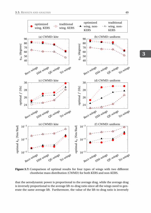
3.5. RESULTS AND ANALYSIS
3
49
Rect-wings
HM-wings
QE-wings
Tri-wings
40
50
60
70
80
90
ηm
[deg
rees
]
(a) CWMD: kite
Rect-wings
HM-wings
QE-wings
Tri-wings
40
50
60
70
80
90
ηm
[deg
rees
]
(b) CWMD: uniform
optimizedwing, KERS
traditionalwing, KERS
optimizedwing, non-KERS
traditionalwing, non-KERS
Rect-wings
HM-wings
QE-wings
Tri-wings
24
26
28
30
op
tim
alf
[Hz]
(c) CWMD: kite
Rect-wings
HM-wings
QE-wings
Tri-wings
24
26
28
30o
pti
mal
f[H
z](d) CWMD: uniform
Rect-wings
HM-wings
QE-wings
Tri-wings10−5
10−4
10−3
op
tim
alkη
[Nm
/Rad
] (e) CWMD: kite
Rect-wings
HM-wings
QE-wings
Tri-wings10−5
10−4
10−3
op
tim
alkη
[Nm
/Rad
] (f ) CWMD: uniform
Figure 3.7: Comparison of optimal results for four types of wings with two differentchordwise mass distribution (CWMD) for both KERS and non-KERS.
that the aerodynamic power is proportional to the average drag, while the average dragis inversely proportional to the average lift-to-drag ratio since all the wings need to gen-erate the same average lift. Furthermore, the value of the lift-to-drag ratio is inversely
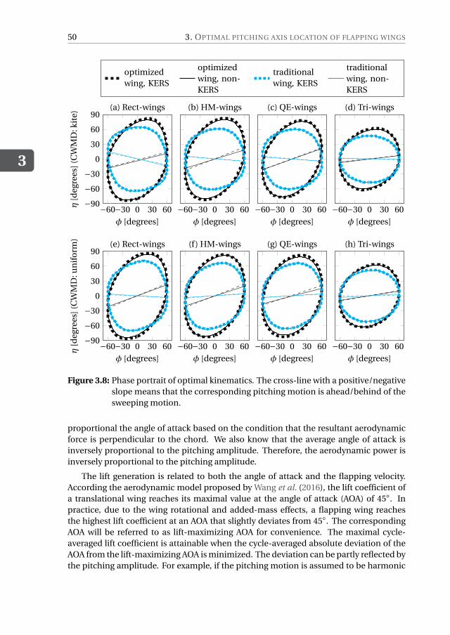
3
50 3. OPTIMAL PITCHING AXIS LOCATION OF FLAPPING WINGS
−60−30 0 30 60−90
−60
−30
0
30
60
90
φ [degrees]
η[d
egre
es](
CW
MD
:kit
e)
(a) Rect-wings
−60−30 0 30 60φ [degrees]
(b) HM-wings
−60−30 0 30 60φ [degrees]
(c) QE-wings
−60−30 0 30 60φ [degrees]
(d) Tri-wings
optimizedwing, KERS
optimizedwing, non-KERS
traditionalwing, KERS
traditionalwing, non-KERS
−60−30 0 30 60−90
−60
−30
0
30
60
90
φ [degrees]
η[d
egre
es](
CW
MD
:un
ifo
rm)
(e) Rect-wings
−60−30 0 30 60φ [degrees]
(f) HM-wings
−60−30 0 30 60φ [degrees]
(g) QE-wings
−60−30 0 30 60φ [degrees]
(h) Tri-wings
Figure 3.8: Phase portrait of optimal kinematics. The cross-line with a positive/negativeslope means that the corresponding pitching motion is ahead/behind of thesweeping motion.
proportional the angle of attack based on the condition that the resultant aerodynamicforce is perpendicular to the chord. We also know that the average angle of attack isinversely proportional to the pitching amplitude. Therefore, the aerodynamic power isinversely proportional to the pitching amplitude.
The lift generation is related to both the angle of attack and the flapping velocity.According the aerodynamic model proposed by Wang et al. (2016), the lift coefficient ofa translational wing reaches its maximal value at the angle of attack (AOA) of 45◦. Inpractice, due to the wing rotational and added-mass effects, a flapping wing reachesthe highest lift coefficient at an AOA that slightly deviates from 45◦. The correspondingAOA will be referred to as lift-maximizing AOA for convenience. The maximal cycle-averaged lift coefficient is attainable when the cycle-averaged absolute deviation of theAOA from the lift-maximizing AOA is minimized. The deviation can be partly reflected bythe pitching amplitude. For example, if the pitching motion is assumed to be harmonic
3.5. RESULTS AND ANALYSIS
3
51
and the lift-maximizing AOA is 45◦, the pitching motion has the minimal deviation whenthe pitching amplitude is 55◦. Therefore, for the wing with a pitching amplitude muchhigher than the lift-maximizing AOA, the average lift coefficient is inversely proportionalto the pitching amplitude. We can see from Fig. 3.7 (a) to Fig. 3.7 (d) that, for the wingwith a higher pitching amplitude (i.e., a smaller average lift coefficient), a higher flap-ping frequency is required to increase the flapping velocity such that the lift constraintcan be satisfied. The frequencies with respect to the optimized HM-wings with a optimalPA location (see Fig. 3.7 (c)) are 27.04 Hz and 26.46 Hz for KERS and non-KERS, respec-tively. In contrast, the average flapping frequency of the reference hawkmoth (Willmott& Ellington, 1997a) is 25.40 Hz. The slightly overestimated frequency can be attributed tothe smaller span and the higher required lift production of the model wing as comparedthe hawkmoth wing (see Table 3.2).
When the PA moves from the LE to the optimal location, the wing pitching inertiadecreases. Meanwhile, the PA gets closer to the center of pressure (CP) which is nor-mally located between the 1/4 chord to the mid-chord (Zhao et al., 2010, Wang et al.,2016). Both the change of the pitching inertia and the distance between the CP and PAtends to reduce the external torque applied on the PA. Therefore, in order to maintainthe expected pitching amplitude, the wing rotational stiffness kη needs to decrease si-multaneously. This is why the optimal stiffness used by wings with a straight LE is muchlarger than that for the wings with a optimal PA location, as shown in Figs. 3.7 (e) and (f).This also provides an explanation to the wing shape and flexibility of insect wings. Witha properly located PA, an insect wing can generate sufficient lift in the most efficient way.Meanwhile, the wing can be very flexible which implies that the structure can be light-weight. The light-weight wing design is also preferred for flapping wings of FWMAVs.
To gain more insight into the pitching motion of wings with the optimal PA, Figure. 3.8shows the phase portraits of their kinematics and the comparison of the optimal kine-matics between optimized and traditional wings. It can be seen that the reversals ofpitching motion with respect to the wing with a optimal PA always take place in advanceto the sweeping reversals. In contrast, the pitching reversals of traditional wings are gen-erally delayed compared to sweeping reversals. The advanced pitching reversal can en-hance the lift generation during the reversal phases (Dickinson et al., 1999, Nakata & Liu,2012b), and it has also been observed on the hovering hawkmoth (Nakata & Liu, 2012b).The PA location might be also one of the explanations to the advanced pitching reversalsobserved for insect flight.
In Figs 3.5, 3.7 and 3.8, we showed the optimal power consumption, design variablesand kinematics for wings with both the kite and uniform profile CWMDs. It can be ob-served that the performance difference between the wings with these two CWMDs ismarginal. For convenience, the analysis presented in this section was primarily basedon the wings with the kite profile CWMD.
3.5.3. INFLUENCE OF LIFT CONSTRAINTS
In order to investigate the dependence of the optimal PA location on the lift constraint,we further optimize the PA location for different lift productions, including 50%, 75%,125% and 150% of the original value (1 g). Taking the HM-wing with a kite profile CWMDas an example, the optimal shapes for different lift constraints are quite close to the orig-
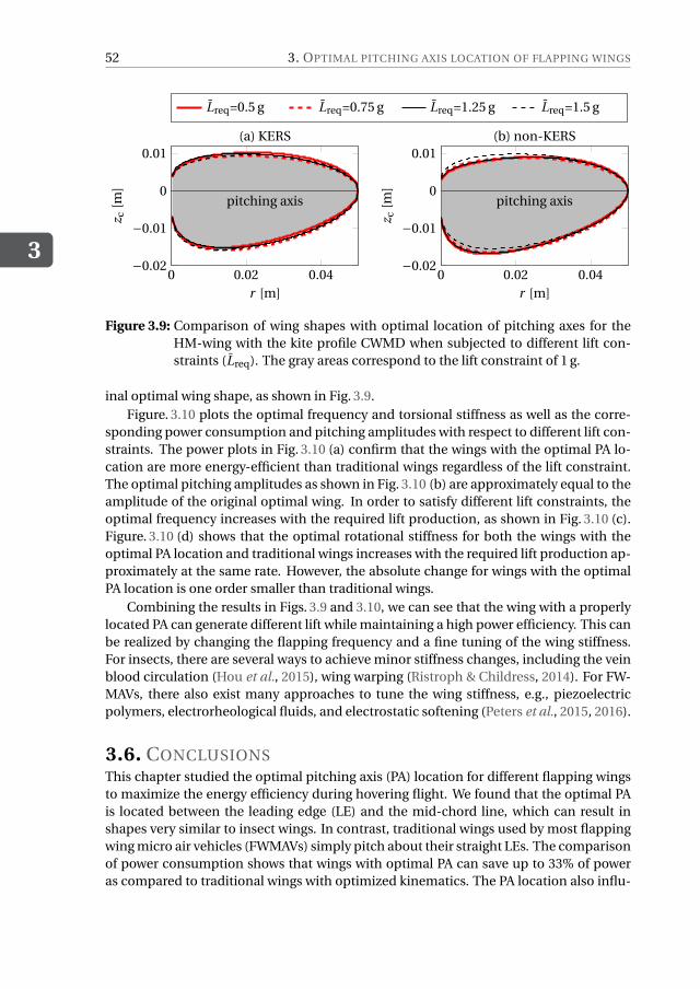
3
52 3. OPTIMAL PITCHING AXIS LOCATION OF FLAPPING WINGS
0 0.02 0.04−0.02
−0.01
0
0.01
pitching axis
r [m]
z c[m
]
(a) KERS
0 0.02 0.04−0.02
−0.01
0
0.01
pitching axis
r [m]
z c[m
]
(b) non-KERS
Lreq=0.5 g Lreq=0.75 g Lreq=1.25 g Lreq=1.5 g
Figure 3.9: Comparison of wing shapes with optimal location of pitching axes for theHM-wing with the kite profile CWMD when subjected to different lift con-straints (Lreq). The gray areas correspond to the lift constraint of 1 g.
inal optimal wing shape, as shown in Fig. 3.9.Figure. 3.10 plots the optimal frequency and torsional stiffness as well as the corre-
sponding power consumption and pitching amplitudes with respect to different lift con-straints. The power plots in Fig. 3.10 (a) confirm that the wings with the optimal PA lo-cation are more energy-efficient than traditional wings regardless of the lift constraint.The optimal pitching amplitudes as shown in Fig. 3.10 (b) are approximately equal to theamplitude of the original optimal wing. In order to satisfy different lift constraints, theoptimal frequency increases with the required lift production, as shown in Fig. 3.10 (c).Figure. 3.10 (d) shows that the optimal rotational stiffness for both the wings with theoptimal PA location and traditional wings increases with the required lift production ap-proximately at the same rate. However, the absolute change for wings with the optimalPA location is one order smaller than traditional wings.
Combining the results in Figs. 3.9 and 3.10, we can see that the wing with a properlylocated PA can generate different lift while maintaining a high power efficiency. This canbe realized by changing the flapping frequency and a fine tuning of the wing stiffness.For insects, there are several ways to achieve minor stiffness changes, including the veinblood circulation (Hou et al., 2015), wing warping (Ristroph & Childress, 2014). For FW-MAVs, there also exist many approaches to tune the wing stiffness, e.g., piezoelectricpolymers, electrorheological fluids, and electrostatic softening (Peters et al., 2015, 2016).
3.6. CONCLUSIONSThis chapter studied the optimal pitching axis (PA) location for different flapping wingsto maximize the energy efficiency during hovering flight. We found that the optimal PAis located between the leading edge (LE) and the mid-chord line, which can result inshapes very similar to insect wings. In contrast, traditional wings used by most flappingwing micro air vehicles (FWMAVs) simply pitch about their straight LEs. The comparisonof power consumption shows that wings with optimal PA can save up to 33% of poweras compared to traditional wings with optimized kinematics. The PA location also influ-
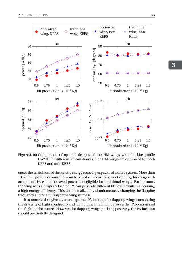
3.6. CONCLUSIONS
3
53
0.5 0.75 1 1.25 1.5
20
30
40
50
60
lift production [×10−3 Kg]
pow
er[W
/Kg]
(a)
0.5 0.75 1 1.25 1.550
60
70
80
90
lift production [×10−3 Kg]o
pti
malη
m[d
egre
es]
(b)
optimizedwing, KERS
traditionalwing, KERS
optimizedwing, non-KERS
traditionalwing, non-KERS
0.5 0.75 1 1.25 1.515
20
25
30
35
lift production [×10−3 Kg]
op
tim
alf
[Hz]
(c)
0.5 0.75 1 1.25 1.510−5
10−4
10−3
lift production [×10−3 Kg]
op
tim
alkη
[Nm
/Rad
]
(d)
Figure 3.10: Comparison of optimal designs of the HM-wings with the kite profileCWMD for different lift constraints. The HM-wings are optimized for bothKERS and non-KERS.
ences the usefulness of the kinetic energy recovery capacity of a drive system. More than13% of the power consumption can be saved via recovering kinetic energy for wings withan optimal PA while the saved power is negligible for traditional wings. Furthermore,the wing with a properly located PA can generate different lift levels while maintaininga high energy efficiency. This can be realized by simultaneously changing the flappingfrequency and fine tuning of the wing stiffness.
It is nontrivial to give a general optimal PA location for flapping wings consideringthe diversity of flight conditions and the nonlinear relation between the PA location andthe flight performance. However, for flapping wings pitching passively, the PA locationshould be carefully designed.

4OPTIMAL TWIST OF FLAPPING
WINGS FOR EFFICIENT HOVERING
FLIGHT
Spanwise twist can dominate the deformation of flapping wings and alters the aerody-namic performance and power efficiency of flapping wings by changing the local angleof attack. Traditional Fluid-Structure Interaction (FSI) models, based on ComputationalStructural Dynamics (CSD) and Computational Fluid Dynamics (CFD), have been usedto investigate the influence of twist on the power efficiency. However, it is impractical touse them for twist optimization due to the high computational cost. On the other hand, itis of great interest to study the optimal twist of flapping wings.
In this chapter, we propose a computationally efficient FSI model based on an analyticaltwist model and a quasi-steady aerodynamic model which replace the expensive CSD andCFD methods. The twist model uses a polynomial to describe the change of the twist an-gle along the span. The polynomial order is determined based on a convergence study. Anonlinear plate model is used to evaluate the structural response of the twisted wing. Theadopted quasi-steady aerodynamic model analytically calculates the aerodynamic loadsby including four loading terms which originate from the wing’s translation, rotation,their coupling and the added-mass effect. Based on the proposed FSI model, we optimizethe twist of a rectangular wing by minimizing the power consumption during hoveringflight. The power efficiency of optimized twistable and rigid wings is studied. This chapteris structured as follows. The introduction is provided in Sec. 4.1. The modeling of twistableflapping wings and the FSI is presented in Sec. 4.2. In Sec. 4.3, the proposed twist modelis validated. In Sec. 4.4, flapping wing twist and kinematics are optimized by minimiz-ing the power consumption for hovering using the proposed FSI model. Conclusions arepresented in Sec. 4.5.
This chapter is based on the paper “Wang, Q., Goosen, J. F. L., & van Keulen, F. An Efficient Fluid-StructureInteraction Model for Optimizing Twistable Flapping Wings. (submitted to Journal of Fluids and Structures”.
55
4
56 4. OPTIMAL TWIST OF FLAPPING WINGS FOR EFFICIENT HOVERING FLIGHT
4.1. INTRODUCTIONFlapping wings keep receiving attention from biologists and engineers due to the in-creasing interest in flapping wing micro air vehicles (FWMAVs). Inspired by insect wings,the kinematics and shape for FWMAV wings have been studied more extensively as com-pared to the wing flexibility.
The wing thickness is typically one to two orders smaller than the wing span and,consequently, insects wings can be modeled as thin-walled structures. The apparentwing flexibility depends on the morphological characteristics, e.g., the venation layout,cross-sectional profile and the membrane thickness. Due to the inertial and aerody-namic loads, dramatic out-of-plane deformation can be observed for some insect wings.The deformation can be decomposed into three modes (Wootton, 1981): spanwise bend-ing, spanwise twist and chordwise camber. For insect wings, the deformation can bedominated by different modes (Willmott & Ellington, 1997a, Chen et al., 2013, Zhenget al., 2013).
For artificial wings, the deformation can also be described by the three modes. Amongthem, the twist is of particular interest for realizing power-efficient wing designs becauseof four reasons. First, to realize the required wing kinematics, the spanwise bendingis normally restricted by the wing structural designs, e.g., using longitudinal stiffeners(Bolsman et al., 2009, de Croon et al., 2009) or chordwise corrugations (Tanaka & Wood,2010, Tanaka, 2012). Second, the turbulent flow surrounding flapping wings is not assensitive as a laminar flow to the wing camber (Du & Sun, 2010). Third, cm-scale flap-ping wings (de Croon et al., 2009, Bolsman et al., 2009) are commonly used for FWMAVs.Such wings can exhibit large twist due to the large difference of the inertial and aerody-namic loads at the wing root and tip. Fourth, the twist can dramatically alter the localangle of attack along the span, which changes the aerodynamic performance and thepower efficiency. Therefore, this work exclusively focuses on the modeling and effectsof wing twist. In addition, only hovering flight is considered because (1) the wing defor-mation is most pronounced during hovering flight (Willmott & Ellington, 1997a), and (2)hovering flight is generally more power-consuming as compared to forward flight (Dud-ley, 2002).
Traditional Fluid-Structure Interaction (FSI) models, based on Computational Struc-tural Dynamics (CSD) and Computational Fluid Dynamics (CFD), have been used to in-vestigate the influence of wing twist on the aerodynamic performance and power ef-ficiency of different flapping wings (Du & Sun, 2008, 2010, Nakata & Liu, 2012a,b, Daiet al., 2012). However, limited by the high computational cost, it is impractical to usethem for twist optimization. The latter is of great interest for the study of insect wingsand the design of artificial wings. Moreover, most of the studies on FSI of flexible wingsprescribed the pitching motion at the root, while in reality passive pitching is widelyused by wings of insects (Ennos, 1989, Bergou et al., 2007) and FWMAVs (de Croon et al.,2009, Bolsman et al., 2009, Ma et al., 2013). The prescribed pitching motion helps thesimulation to converge easier and reduces the computational cost. However, the powerconsumption of flapping wings with prescribed and passive pitching motion can differdramatically (Han et al., 2015). In this work, we propose a computationally efficient FSImodel to study the (optimal) twist of flapping wings. The proposed FSI model uses ananalytical twist model for the structural analysis and a quasi-steady aerodynamic model
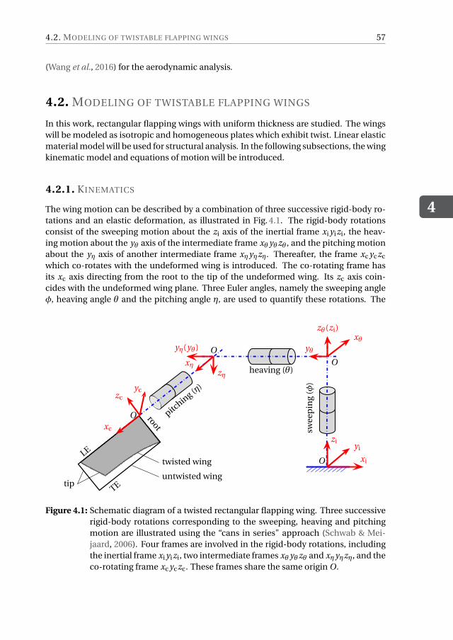
4.2. MODELING OF TWISTABLE FLAPPING WINGS
4
57
(Wang et al., 2016) for the aerodynamic analysis.
4.2. MODELING OF TWISTABLE FLAPPING WINGS
In this work, rectangular flapping wings with uniform thickness are studied. The wingswill be modeled as isotropic and homogeneous plates which exhibit twist. Linear elasticmaterial model will be used for structural analysis. In the following subsections, the wingkinematic model and equations of motion will be introduced.
4.2.1. KINEMATICS
The wing motion can be described by a combination of three successive rigid-body ro-tations and an elastic deformation, as illustrated in Fig. 4.1. The rigid-body rotationsconsist of the sweeping motion about the zi axis of the inertial frame xi yizi, the heav-ing motion about the yθ axis of the intermediate frame xθyθzθ , and the pitching motionabout the yη axis of another intermediate frame xηyηzη. Thereafter, the frame xc yczc
which co-rotates with the undeformed wing is introduced. The co-rotating frame hasits xc axis directing from the root to the tip of the undeformed wing. Its zc axis coin-cides with the undeformed wing plane. Three Euler angles, namely the sweeping angleφ, heaving angle θ and the pitching angle η, are used to quantify these rotations. The
O xi
yizi
O
xθyθ
zθ(zi)
O
xη
yη(yθ)
zη
Oxc
yczc
swee
pin
g(φ
)
heaving (θ)
pitchin
g (η)
LE
TE
root
tipuntwisted wing
twisted wing
Figure 4.1: Schematic diagram of a twisted rectangular flapping wing. Three successiverigid-body rotations corresponding to the sweeping, heaving and pitchingmotion are illustrated using the “cans in series" approach (Schwab & Mei-jaard, 2006). Four frames are involved in the rigid-body rotations, includingthe inertial frame xi yizi, two intermediate frames xθyθzθ and xηyηzη, and theco-rotating frame xc yczc. These frames share the same origin O.
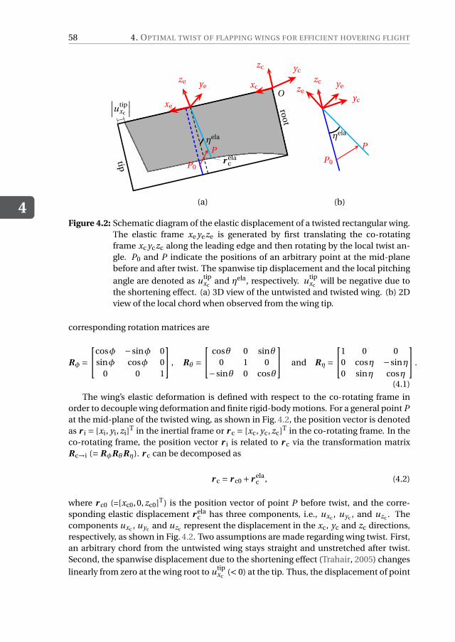
4
58 4. OPTIMAL TWIST OF FLAPPING WINGS FOR EFFICIENT HOVERING FLIGHT
xc
yczc
O∣∣∣utipxc
∣∣∣ xe
yeze
P0
Pr ela
croot
tip
ηela ηela
P0
P
yc
zcze
ye
(a) (b)
Figure 4.2: Schematic diagram of the elastic displacement of a twisted rectangular wing.The elastic frame xe yeze is generated by first translating the co-rotatingframe xc yczc along the leading edge and then rotating by the local twist an-gle. P0 and P indicate the positions of an arbitrary point at the mid-planebefore and after twist. The spanwise tip displacement and the local pitching
angle are denoted as utipxc
and ηela, respectively. utipxc
will be negative due tothe shortening effect. (a) 3D view of the untwisted and twisted wing. (b) 2Dview of the local chord when observed from the wing tip.
corresponding rotation matrices are
Rφ =
cosφ −sinφ 0sinφ cosφ 0
0 0 1
, Rθ =
cosθ 0 sinθ0 1 0
−sinθ 0 cosθ
and Rη =
1 0 00 cosη −sinη0 sinη cosη
.
(4.1)
The wing’s elastic deformation is defined with respect to the co-rotating frame inorder to decouple wing deformation and finite rigid-body motions. For a general point Pat the mid-plane of the twisted wing, as shown in Fig. 4.2, the position vector is denotedas r i = [xi, yi, zi]T in the inertial frame or r c = [xc, yc, zc]T in the co-rotating frame. In theco-rotating frame, the position vector r i is related to r c via the transformation matrixRc→i (= RφRθRη). r c can be decomposed as
r c = r c0 + r elac , (4.2)
where r c0 (=[xc0,0, zc0]T) is the position vector of point P before twist, and the corre-sponding elastic displacement r ela
c has three components, i.e., uxc , uyc , and uzc . Thecomponents uxc , uyc and uzc represent the displacement in the xc, yc and zc directions,respectively, as shown in Fig. 4.2. Two assumptions are made regarding wing twist. First,an arbitrary chord from the untwisted wing stays straight and unstretched after twist.Second, the spanwise displacement due to the shortening effect (Trahair, 2005) changes
linearly from zero at the wing root to utipxc
(< 0) at the tip. Thus, the displacement of point
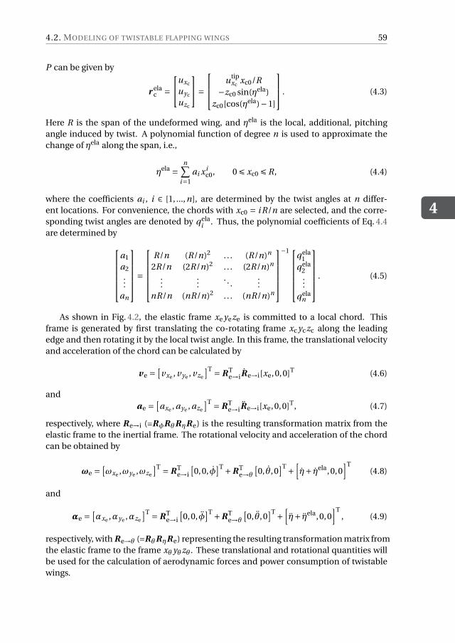
4.2. MODELING OF TWISTABLE FLAPPING WINGS
4
59
P can be given by
r elac =
uxc
uyc
uzc
=
utipxc
xc0/R−zc0 sin(ηela)
zc0[cos(ηela)−1]
. (4.3)
Here R is the span of the undeformed wing, and ηela is the local, additional, pitchingangle induced by twist. A polynomial function of degree n is used to approximate thechange of ηela along the span, i.e.,
ηela =n∑
i=1ai xi
c0, 0 É xc0 É R, (4.4)
where the coefficients ai , i ∈ [1, ...,n], are determined by the twist angles at n differ-ent locations. For convenience, the chords with xc0 = i R/n are selected, and the corre-sponding twist angles are denoted by qela
i . Thus, the polynomial coefficients of Eq. 4.4are determined by
a1
a2...
an
=
R/n (R/n)2 . . . (R/n)n
2R/n (2R/n)2 . . . (2R/n)n
......
. . ....
nR/n (nR/n)2 . . . (nR/n)n
−1
qela1
qela2...
qelan
. (4.5)
As shown in Fig. 4.2, the elastic frame xe yeze is committed to a local chord. Thisframe is generated by first translating the co-rotating frame xc yczc along the leadingedge and then rotating it by the local twist angle. In this frame, the translational velocityand acceleration of the chord can be calculated by
v e =[vxe , vye , vze
]T = RTe→iRe→i[xe,0,0]T (4.6)
andae =
[axe , aye , aze
]T = RTe→iRe→i[xe,0,0]T, (4.7)
respectively, where Re→i (=RφRθRηRe) is the resulting transformation matrix from theelastic frame to the inertial frame. The rotational velocity and acceleration of the chordcan be obtained by
ωe =[ωxe ,ωye ,ωze
]T = RTe→i
[0,0, φ
]T +RTe→θ
[0, θ,0
]T +[η+ ηela,0,0
]T(4.8)
and
αe =[αxe ,αye ,αze
]T = RTe→i
[0,0, φ
]T +RTe→θ
[0, θ,0
]T +[η+ ηela,0,0
]T, (4.9)
respectively, with Re→θ (=RθRηRe) representing the resulting transformation matrix fromthe elastic frame to the frame xθyθzθ. These translational and rotational quantities willbe used for the calculation of aerodynamic forces and power consumption of twistablewings.
4
60 4. OPTIMAL TWIST OF FLAPPING WINGS FOR EFFICIENT HOVERING FLIGHT
4.2.2. EQUATIONS OF MOTION
The generalized coordinates that determine the wing kinematics include
q =[[
q rot]T,[
q ela]T
]T
, (4.10)
where q rot (= [qrot1 , qrot
2 , qrot3 ]T) and q ela (= [qela
1 , qela2 , ..., qela
n , qelan+1]T) are associated to the
wing rigid-body rotations and the elastic deformation, respectively. For convenience,q rot and q ela will be referred to as rotational and elastic generalized coordinates, respec-tively. The first n coordinates of q ela have been introduced in Eq. 4.5. The coordinatesqrot
1 , qrot2 , qrot
3 and qelan+1 represent the sweeping angle φ, heaving angle θ, pitching angle
η and the spanwise tip displacement utipxc
, respectively.The wing’s equations of motion can be derived from Lagrange’s equation
d
d t
(∂Ek
∂q
)− ∂Ek
∂q+ ∂Ep
∂q=Qext, (4.11)
with Ek and Ep representing the wing’s kinetic and potential energy, respectively, andQext the generalized forces related to the external drive and aerodynamic loads.
KINETIC ENERGY
The wing’s kinetic energy can be calculated by
Ek =1
2
Ï
Shρwr T
i r id s = 1
2
Ï
Shρw (
Lq)T Lqd s ,
1
2q TM wq , (4.12)
where h is the wing thickness, S is the area of the untwisted wing, ρw is the wing density,and M w is the wing’s mass matrix. M w is given by
M w =Ï
ShρwLTLd s, (4.13)
with
L =[∂ (Rc→ir c)
∂q rot ,Rc→i∂r c
∂q ela
]. (4.14)
Substituting the kinetic energy (Eq. 4.12) into the first two terms at the left-hand sideof the Lagrange’s equation (Eq. 4.11) yields
d
d t
(∂Ek
∂q
)− ∂Ek
∂q= M wq +Qv, (4.15)
where Qv represents the sum of the centrifugal and Coriolis forces, i.e.,
Qv = M wq −[∂
∂q
(1
2q TM wq
)]T
. (4.16)
4.2. MODELING OF TWISTABLE FLAPPING WINGS
4
61
ELASTIC POTENTIAL ENERGY
Typically, the pitching motion of flapping wings results from both the torsion/bending ofthe elastic elements at the wing root (e.g., torsional spring, elastic hinge or slender beam)and the deformation of the wing plate. These two contributions are functions of thegeneralized coordinates q rot and q ela, respectively. Therefore, the total wing potentialenergy can be decomposed into
Ep = E rotp
(q rot)+E ela
p
(q ela
), (4.17)
with E rotp and E ela
p representing the elastic energy related to the rigid-body rotations andthe elastic wing twist, respectively. By assuming linear elastic root elements (Howell,2001, Whitney & Wood, 2010, Wang et al., 2014a), E rot
p can be formulated as
E rotp = 1
2
[q rot]T
K rotq rot, (4.18)
where K rot represents the stiffness matrix associated to the rigid-body rotations. Basedon the linear elastic material model, the potential energy E ela
p can be calculated by
E elap = 1
2
Ñ
VεT Cεd v, (4.19)
of which V is the wing volume, ε is the wing strain, and C is the matrix with elastic co-efficient. Nonlinear strain-displacement relations for plates with moderate deformationare used to calculate the strain, as given by
ε=εxc0
εzc0
γxc0zc0
=
∂uxc∂xc
+ 12
(∂uxc∂xc
)2+ 1
2
(∂uzc∂xc
)2+ 1
2
(∂uyc∂xc
)2− yc
∂2uyc
∂x2c
∂uzc∂zc
+ 12
(∂uxc∂zc
)2+ 1
2
(∂uzc∂zc
)2+ 1
2
(∂uyc∂zc
)2− yc
∂2uyc
∂z2c
∂uzc∂xc
+ ∂uxc∂zc
+ ∂uxc∂zc
∂uxc∂xc
+ ∂uzc∂zc
∂uzc∂xc
+ ∂uyc∂zc
∂uyc∂xc
−2yc∂2uyc∂xc∂zc
, (4.20)
where ε and γ represent the normal and shear strain, respectively. It can be observedthat Kirchhoff’s hypothesis is used and quadratic membrane strain terms are included.The importance of these nonlinear strain terms increases with the twist angle. The con-stitutive matrix in Eq. 4.19 is given by
C = E
1−ν2
1 ν 0ν 1 00 0 (1−ν)/2
, (4.21)
with E and ν representing the Young’s modulus and Poisson’s ratio of the wing, respec-tively.
Knowing E rotp and E ela
p ,∂Ep
∂q can be calculated. The derivative physically represents
the generalized elastic force. If the generalized elastic force is denoted as Qela, we get
∂Ep
∂q=Qela. (4.22)
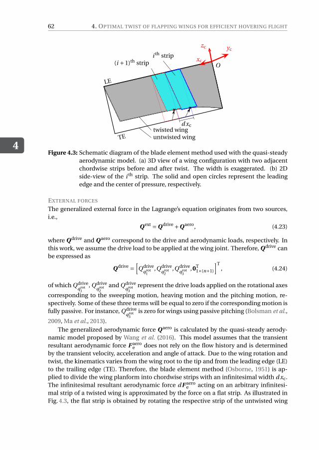
4
62 4. OPTIMAL TWIST OF FLAPPING WINGS FOR EFFICIENT HOVERING FLIGHT
xc
yczc
O
untwisted wingtwisted wing
TE
LE
(i +1)th stripi th strip
d xc
Figure 4.3: Schematic diagram of the blade element method used with the quasi-steadyaerodynamic model. (a) 3D view of a wing configuration with two adjacentchordwise strips before and after twist. The width is exaggerated. (b) 2Dside-view of the i th strip. The solid and open circles represent the leadingedge and the center of pressure, respectively.
EXTERNAL FORCES
The generalized external force in the Lagrange’s equation originates from two sources,i.e.,
Qext =Qdrive +Qaero, (4.23)
where Qdrive and Qaero correspond to the drive and aerodynamic loads, respectively. Inthis work, we assume the drive load to be applied at the wing joint. Therefore, Qdrive canbe expressed as
Qdrive =[Qdrive
qrot1
,Qdriveqrot
2,Qdrive
qrot3
,0T1×(n+1)
]T, (4.24)
of which Qdriveqrot
1, Qdrive
qrot2
and Qdriveqrot
3represent the drive loads applied on the rotational axes
corresponding to the sweeping motion, heaving motion and the pitching motion, re-spectively. Some of these three terms will be equal to zero if the corresponding motion isfully passive. For instance, Qdrive
qrot3
is zero for wings using passive pitching (Bolsman et al.,
2009, Ma et al., 2013).The generalized aerodynamic force Qaero is calculated by the quasi-steady aerody-
namic model proposed by Wang et al. (2016). This model assumes that the transientresultant aerodynamic force F aero
e does not rely on the flow history and is determinedby the transient velocity, acceleration and angle of attack. Due to the wing rotation andtwist, the kinematics varies from the wing root to the tip and from the leading edge (LE)to the trailing edge (TE). Therefore, the blade element method (Osborne, 1951) is ap-plied to divide the wing planform into chordwise strips with an infinitesimal width d xc.The infinitesimal resultant aerodynamic force dF aero
e acting on an arbitrary infinitesi-mal strip of a twisted wing is approximated by the force on a flat strip. As illustrated inFig. 4.3, the flat strip is obtained by rotating the respective strip of the untwisted wing
4.2. MODELING OF TWISTABLE FLAPPING WINGS
4
63
by the local twist angle. The tip displacement utipxc
due to the shortening effect is typi-cally two orders smaller than the original span for a moderately twisted wing. Therefore,the change of the wing span due to the twist is neglected for the aerodynamic analysis.The quasi-steady aerodynamic model assumes the resultant force to be perpendicularto the local flat strip considering the pressure load dominates the aerodynamic load onflapping wings (Wang et al., 2016). Therefore, dF aero
e can be expressed as
dF aeroe = dF aero
yee ye , (4.25)
with e ye denoting the unit vector in the direction of the ye axis of the elastic frame. Thequasi-steady model calculates the magnitude of dF aero
yeby including four loading terms:
dF aeroye
=(F trans
ye+ F rot
ye+ F coupl
ye+ F am
ye
)d xe, (4.26)
where F transye
, F rotye
, F couplye
and F amye
represent the force components resulting from thetranslation, rotation, their coupling and the added-mass effect of a strip of unit width,respectively. The detailed expressions of these forces are provided in Chapter 2. Thegeneralized aerodynamic force for the entire wing can be obtained by
Qaero =∫ R
0
{F trans
ye
[∂r trans
i,cp
∂q
]T
+ F rotye
[∂r rot
i,cp
∂q
]T
+ F couplye
∂r coupl
i,cp
∂q
T
+ F amye
[∂r am
i,cp
∂q
]T }Re→ie ye d xe, (4.27)
with r transi,cp , r rot
i,cp, r coupli,cp and r am
i,cp representing the position vectors of the centers of pres-sure in the inertial frame. These vectors can be obtained by
r ⊕i,cp = Re→i[xe,0,−cd⊕
cp]T, (4.28)
with the superscript “⊕” referring to “trans”, “rot”, “coupl” or “am” for the different load-
ing terms. The locations of the centers of pressure d transcp , d rot
cp , d couplcp and d am
cp are alsoprovided in Chapter 2.
The first three components of Qaero are functions of the generalized velocities, butthe last term (i.e., the added-mass term) can be separated into two parts which are func-tions of the generalized velocities and accelerations, respectively. Therefore, Qaero canbe rewritten as
Qaero = Qaero −M amq . (4.29)
Here, Qaero
includes all the generalized velocity related terms, and M am is the mass ma-trix related to the added-mass effect.
Substituting Eqs. 4.15, 4.22, 4.23 and 4.29 into the Lagrange’s equation in Eq. 4.11, wecan obtain the equations of motion for a twistable wing as in
M q =−Qela +Qdrive +Qaero −Qv, (4.30)
where M(= M w +M am) is the effective mass matrix.
4
64 4. OPTIMAL TWIST OF FLAPPING WINGS FOR EFFICIENT HOVERING FLIGHT
4.2.3. KINEMATIC CONSTRAINTSFor insects and FWMAVs, there might exist kinematic constraints on the wing rigid-bodyrotations. For instance, the sweeping motion is generally controlled by a drive system,and a certain type of heaving motion or no heaving motion is generally enforced. If thereare nc rotational constraints, the number of independent generalized coordinates ni willbe n+4−nc. The equations of motion given by Eq. 4.30 can be rewritten in a partitionedform as
[M nc×nc M nc×ni
M ni×nc M ni×ni
][q nc×1q ni×1
]=−
[0
Qelani×1
]+
[Qdrive
nc×10
]+
[Q
aeronc×1
Qaeroni×1
]−
[Qv
nc×1Qv
ni×1
], (4.31)
of which the unknown terms are q ni×1 and Qdrivenc×1. Therefore, two set of equations can be
obtained, namely
Qdrivenc×1 = M nc×nc q nc×1 +M nc×ni q ni×1 −Q
aeronc×1 +Qv
nc×1, (4.32)
andM ni×ni q ni×1 =−Qela
ni×1 +Qaeroni×1 −Qv
ni×1 −M ni×nc q nc×1. (4.33)
The latter equation represents the set of independent equations of motion. The last termin its right-hand side refers to the Euler force due to the prescribed rotational accelera-tion. By solving Eq. 4.33, the motion of a twistable wing can be obtained. SubstitutingEq. 4.33 into Eq. 4.32, we get
Qdrivenc×1 =
[M nc×nc −M nc×ni M−1
ni×niM ni×nc
]q nc×1 −M nc×ni M−1
ni×niQv
ni×1 +Qvnc×1︸ ︷︷ ︸
inertial terms
+M nc×ni M−1ni×ni
Qaeroni×1 −Q
aeronc×1︸ ︷︷ ︸
aerodynamicterms
−M nc×ni M−1ni×ni
Qelani×1︸ ︷︷ ︸
elasticterms
, (4.34)
from which it can seen that Qdrivenc×1 is used to accelerate/decelerate the wing, overcome
the aerodynamic drag and resist the elastic force, as represented by the inertial, aero-dynamic and elastic terms, respectively. In practice, Qdrive
nc×1 is the drive torque which isapplied by the motor of FWMAVs or the thorax of insects. It can be used to determinethe power consumption.
4.3. VALIDATION OF THE PROPOSED TWIST MODELTo validate the proposed twist model, we set the span, aspect ratio and the mass of therectangular wing as 50 mm, 2.5 and 50 mg, respectively, by referring to the adult hawk-moth (HMF2) (Willmott & Ellington, 1997b) and artificial wings of similar size (Bols-man et al., 2009). The wing thickness is set as 1 mm. Here the average thickness ofthe wing of HMF2 (about 35µm) is not referred to for two reasons. First, the averagethickness is not adequate to reflect the real hawkmoth wing thickness distribution con-sidering its morphological complexity. Second, the wing with prescribed dimensionsand mass can be easily fabricated using a foam sheet (Expanded PolyStyrene) in case ar-tificial wings are needed for futural experimental study. A harmonic sweeping motion,φ(t ) = φm sin(2π f t ), is applied to drive the wing, where the amplitude φm is set to 60◦
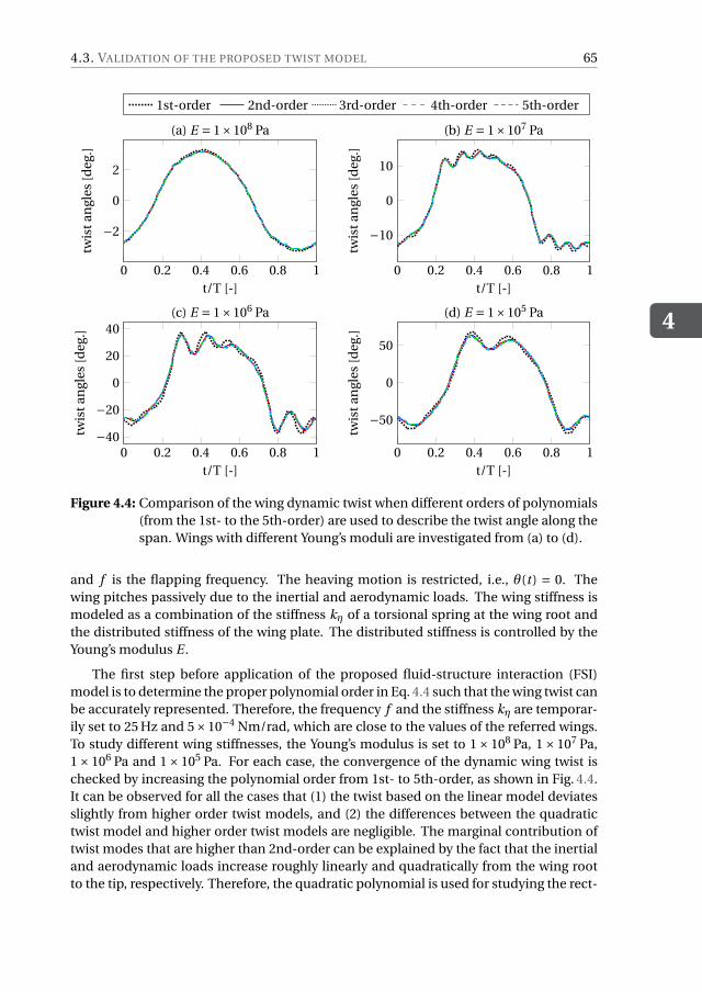
4.3. VALIDATION OF THE PROPOSED TWIST MODEL
4
65
0 0.2 0.4 0.6 0.8 1
−2
0
2
t/T [-]
twis
tan
gles
[deg
.]
(a) E = 1×10⁸ Pa
0 0.2 0.4 0.6 0.8 1
−10
0
10
t/T [-]
twis
tan
gles
[deg
.]
(b) E = 1×10⁷ Pa
1st-order 2nd-order 3rd-order 4th-order 5th-order
0 0.2 0.4 0.6 0.8 1−40
−20
0
20
40
t/T [-]
twis
tan
gles
[deg
.]
(c) E = 1×10⁶ Pa
0 0.2 0.4 0.6 0.8 1
−50
0
50
t/T [-]
twis
tan
gles
[deg
.]
(d) E = 1×10⁵ Pa
Figure 4.4: Comparison of the wing dynamic twist when different orders of polynomials(from the 1st- to the 5th-order) are used to describe the twist angle along thespan. Wings with different Young’s moduli are investigated from (a) to (d).
and f is the flapping frequency. The heaving motion is restricted, i.e., θ(t ) = 0. Thewing pitches passively due to the inertial and aerodynamic loads. The wing stiffness ismodeled as a combination of the stiffness kη of a torsional spring at the wing root andthe distributed stiffness of the wing plate. The distributed stiffness is controlled by theYoung’s modulus E .
The first step before application of the proposed fluid-structure interaction (FSI)model is to determine the proper polynomial order in Eq. 4.4 such that the wing twist canbe accurately represented. Therefore, the frequency f and the stiffness kη are temporar-ily set to 25 Hz and 5×10⁻⁴ Nm/rad, which are close to the values of the referred wings.To study different wing stiffnesses, the Young’s modulus is set to 1× 10⁸ Pa, 1× 10⁷ Pa,1× 106 Pa and 1× 10⁵ Pa. For each case, the convergence of the dynamic wing twist ischecked by increasing the polynomial order from 1st- to 5th-order, as shown in Fig. 4.4.It can be observed for all the cases that (1) the twist based on the linear model deviatesslightly from higher order twist models, and (2) the differences between the quadratictwist model and higher order twist models are negligible. The marginal contribution oftwist modes that are higher than 2nd-order can be explained by the fact that the inertialand aerodynamic loads increase roughly linearly and quadratically from the wing rootto the tip, respectively. Therefore, the quadratic polynomial is used for studying the rect-
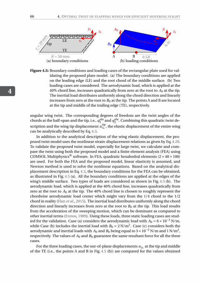
4
66 4. OPTIMAL TWIST OF FLAPPING WINGS FOR EFFICIENT HOVERING FLIGHT
xi
yi zi
TE
LEtip
(a) boundary conditions
c =20
mm
R = 50 mm
xi
yi zi
(b) loading conditions
B0
A0
A B
0.4c
0.5R
Figure 4.5: Boundary conditions and loading cases of the rectangular plate used for val-idating the proposed plate model. (a) The boundary conditions are appliedon the leading edge (LE) and the root chord of the middle surface. (b) Twoloading cases are considered. The aerodynamic load, which is applied at the40% chord line, increases quadratically from zero at the root to A0 at the tip.The inertial load distributes uniformly along the chord direction and linearlyincreases from zero at the root to B0 at the tip. The points A and B are locatedat the tip and middle of the trailing edge (TE), respectively.
angular wing twist. The corresponding degrees of freedom are the twist angles of thechords at the half-span and the tip, i.e., qela
1 and qela2 . Combining this quadratic twist de-
scription and the wing tip displacement utipxc
, the elastic displacement of the entire wingcan be analytically described by Eq. 4.3.
In addition to the analytical description of the wing elastic displacement, the pro-posed twist model uses the nonlinear strain-displacement relations as given by Eq. 4.20.To validate the proposed twist model, especially for large twist, we calculate and com-pare the twist using both the proposed model and a finite element analysis (FEA) usingCOMSOL Multiphysics® software. In FEA, quadratic hexahedral elements (2×40×100)are used. For both the FEA and the proposed model, linear elasticity is assumed, andNewton method is used to solve the nonlinear equations. Based on the analytical dis-placement description in Eq. 4.3, the boundary conditions for the FEA can be obtained,as illustrated in Fig. 4.5 (a). All the boundary conditions are applied at the edges of thewing’s middle surface. Two types of loads are considered as shown in Fig. 4.5 (b). Theaerodynamic load, which is applied at the 40% chord line, increases quadratically fromzero at the root to A0 at the tip. The 40% chord line is chosen to roughly represent thechordwise aerodynamic load center which might vary from the 1/4 chord to the 1/2chord in reality (Han et al., 2015). The inertial load distributes uniformly along the chorddirection and linearly increases from zero at the root to B0 at the tip. This load resultsfrom the acceleration of the sweeping motion, which can be dominant as compared toother inertial terms (Ennos, 1989). Using these loads, three static loading cases are stud-ied for the validation. Case (a) considers the aerodynamic load with A0 = 6×10⁻² N/m,while Case (b) includes the inertial load with B0 = 2 N/m2. Case (c) considers both theaerodynamic and inertial loads with A0 and B0 being equal to 3×10⁻² N/m and 1 N/m2,respectively. The values of A0 and B0 guarantee the same resultant force for all the threecases.
For the three loading cases, the out-of-plane displacements uyc at the tip and middleof the TE (i.e., the points A and B in Fig. 4.5 (b)) are compared for the values obtained
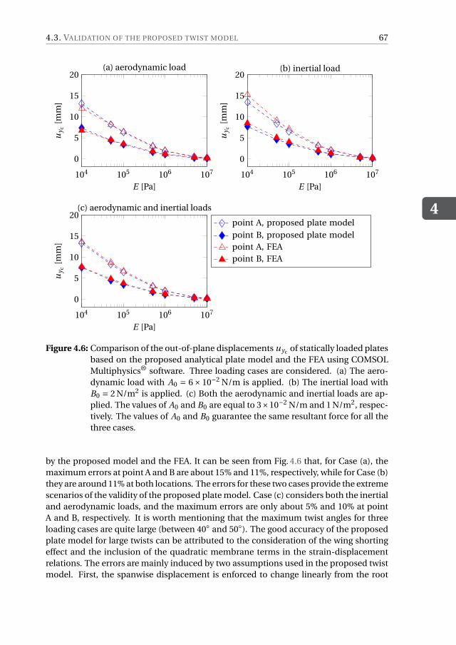
4.3. VALIDATION OF THE PROPOSED TWIST MODEL
4
67
104 105 106 107
0
5
10
15
20
E [Pa]
uy c
[mm
](a) aerodynamic load
104 105 106 107
0
5
10
15
20
E [Pa]
uy c
[mm
]
(b) inertial load
104 105 106 107
0
5
10
15
20
E [Pa]
uy c
[mm
]
(c) aerodynamic and inertial loads
point A, proposed plate modelpoint B, proposed plate modelpoint A, FEApoint B, FEA
Figure 4.6: Comparison of the out-of-plane displacements uyc of statically loaded platesbased on the proposed analytical plate model and the FEA using COMSOLMultiphysics® software. Three loading cases are considered. (a) The aero-dynamic load with A0 = 6× 10⁻² N/m is applied. (b) The inertial load withB0 = 2 N/m2 is applied. (c) Both the aerodynamic and inertial loads are ap-plied. The values of A0 and B0 are equal to 3×10⁻² N/m and 1 N/m2, respec-tively. The values of A0 and B0 guarantee the same resultant force for all thethree cases.
by the proposed model and the FEA. It can be seen from Fig. 4.6 that, for Case (a), themaximum errors at point A and B are about 15% and 11%, respectively, while for Case (b)they are around 11% at both locations. The errors for these two cases provide the extremescenarios of the validity of the proposed plate model. Case (c) considers both the inertialand aerodynamic loads, and the maximum errors are only about 5% and 10% at pointA and B, respectively. It is worth mentioning that the maximum twist angles for threeloading cases are quite large (between 40◦ and 50◦). The good accuracy of the proposedplate model for large twists can be attributed to the consideration of the wing shortingeffect and the inclusion of the quadratic membrane terms in the strain-displacementrelations. The errors are mainly induced by two assumptions used in the proposed twistmodel. First, the spanwise displacement is enforced to change linearly from the root
4
68 4. OPTIMAL TWIST OF FLAPPING WINGS FOR EFFICIENT HOVERING FLIGHT
to the tip. Second, the chordwise stretching and camber are ignored. In contrast, theFEA shows a more complicated spanwise displacement field due to the varying spanwiseshortening from the LE to the TE. Meanwhile, significant camber can be observed whenthe wing is subject to the prescribed aerodynamic loads.
4.4. TWIST OPTIMIZATIONThe proposed twist model and the quasi-steady aerodynamic model dramatically re-duce the computational cost for the FSI analysis as compared to traditional FSI models.In our FSI simulations, the wing is discretized into 50 chordwise strips, which are ade-quate for the description of the quadratic wing twist. The wing’s passive pitching motionnormally starts to converge to its steady state from the second half of the first cycle. Theaerodynamic force and power consumption in the third cycle are used for analysis andoptimization. Newmark method with γ= 1/2 and β= 1/4 is used to solve the equationsof motion while 500 time steps are taken for each cycle. Each simulation takes aboutonly 4 minutes when using MATLAB® R2014b on a 64-bit computer with a RAM capacityof 8 GB and an Intel® CoreTM i5 CPU at 3.40 GHz.
4.4.1. OPTIMIZATION MODEL
The proposed FSI model will be used to optimize the wing twist and kinematics whichminimize the cycle-averaged power consumption during hovering flight. The designvariables include the root stiffness kη, the Young’s modulus E and the flapping frequencyf . The power can be calculated by
P total = q Tnc×1Qdrive
nc×1, (4.35)
where Qdrivenc×1 and q nc×1 are the drive torque and generalized velocity, respectively. Sim-
ilar to Eq. 4.34, the total power can be decomposed into three components, namely theaerodynamic power P aero, inertial power P iner and the elastic power P ela. Note, thepower can be negative due to the loss of the kinetic energy during the deceleration. Thelost kinetic energy can be dissipated, used to compensate the energy consumed by theaerodynamic drag, or stored in a kinetic energy recovery drive system (KERS). KERS canappear in different forms, e.g., insect thoraxes (Dudley, 2002) and elastic structures ofFWMAVs (Bolsman et al., 2009, Lau et al., 2014). The uncertainty in the kinetic energytransformation complicates the modeling of the average power consumption. Instead,two extreme power consumption scenarios are modeled. First, an ideal KERS is used,which implies that the average elastic and inertia power are both zero. In this setting,the total average power is equal to the average aerodynamic power, i.e.,
P totalKERS =
1
T
∫
TP totald t = 1
T
∫
TP aerod t , (4.36)
with T representing the period of a flapping cycle. Second, a drive system which can notrecover any energy is adopted. In this case, the kinetic and elastic energy first compen-sate the energy consumed by drag. Then, extra energy will be dissipated. This type ofdrive system will be referred to as non-KERS. The total average power for this extreme
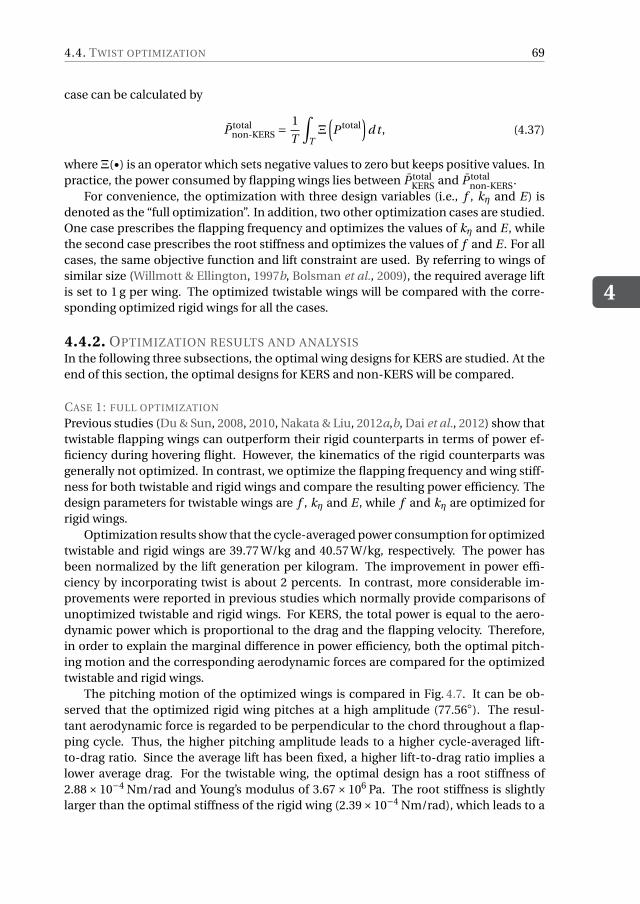
4.4. TWIST OPTIMIZATION
4
69
case can be calculated by
P totalnon-KERS =
1
T
∫
TΞ
(P total
)d t , (4.37)
whereΞ(•) is an operator which sets negative values to zero but keeps positive values. Inpractice, the power consumed by flapping wings lies between P total
KERS and P totalnon-KERS.
For convenience, the optimization with three design variables (i.e., f , kη and E) isdenoted as the “full optimization”. In addition, two other optimization cases are studied.One case prescribes the flapping frequency and optimizes the values of kη and E , whilethe second case prescribes the root stiffness and optimizes the values of f and E . For allcases, the same objective function and lift constraint are used. By referring to wings ofsimilar size (Willmott & Ellington, 1997b, Bolsman et al., 2009), the required average liftis set to 1 g per wing. The optimized twistable wings will be compared with the corre-sponding optimized rigid wings for all the cases.
4.4.2. OPTIMIZATION RESULTS AND ANALYSISIn the following three subsections, the optimal wing designs for KERS are studied. At theend of this section, the optimal designs for KERS and non-KERS will be compared.
CASE 1: FULL OPTIMIZATION
Previous studies (Du & Sun, 2008, 2010, Nakata & Liu, 2012a,b, Dai et al., 2012) show thattwistable flapping wings can outperform their rigid counterparts in terms of power ef-ficiency during hovering flight. However, the kinematics of the rigid counterparts wasgenerally not optimized. In contrast, we optimize the flapping frequency and wing stiff-ness for both twistable and rigid wings and compare the resulting power efficiency. Thedesign parameters for twistable wings are f , kη and E , while f and kη are optimized forrigid wings.
Optimization results show that the cycle-averaged power consumption for optimizedtwistable and rigid wings are 39.77 W/kg and 40.57 W/kg, respectively. The power hasbeen normalized by the lift generation per kilogram. The improvement in power effi-ciency by incorporating twist is about 2 percents. In contrast, more considerable im-provements were reported in previous studies which normally provide comparisons ofunoptimized twistable and rigid wings. For KERS, the total power is equal to the aero-dynamic power which is proportional to the drag and the flapping velocity. Therefore,in order to explain the marginal difference in power efficiency, both the optimal pitch-ing motion and the corresponding aerodynamic forces are compared for the optimizedtwistable and rigid wings.
The pitching motion of the optimized wings is compared in Fig. 4.7. It can be ob-served that the optimized rigid wing pitches at a high amplitude (77.56◦). The resul-tant aerodynamic force is regarded to be perpendicular to the chord throughout a flap-ping cycle. Thus, the higher pitching amplitude leads to a higher cycle-averaged lift-to-drag ratio. Since the average lift has been fixed, a higher lift-to-drag ratio implies alower average drag. For the twistable wing, the optimal design has a root stiffness of2.88× 10−4 Nm/rad and Young’s modulus of 3.67× 10⁶ Pa. The root stiffness is slightlylarger than the optimal stiffness of the rigid wing (2.39×10⁻⁴ Nm/rad), which leads to a
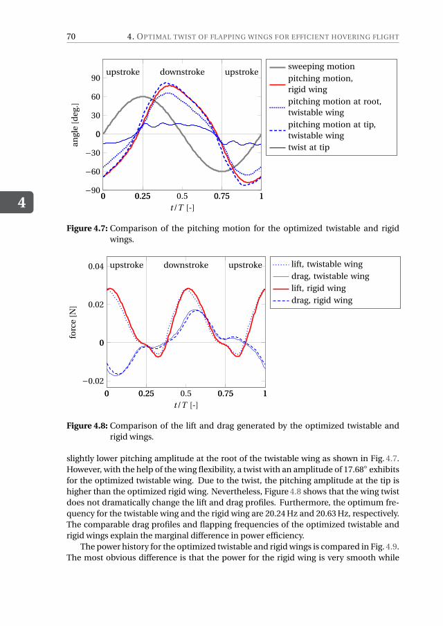
4
70 4. OPTIMAL TWIST OF FLAPPING WINGS FOR EFFICIENT HOVERING FLIGHT
0 0.25 0.5 0.75 1−90
−60
−30
0
30
60
90
0 0.25 0.75 1
0
upstroke downstroke upstroke
t/T [-]
angl
e[d
eg.]
sweeping motion
pitching motion,rigid wing
pitching motion at root,twistable wing
pitching motion at tip,twistable wingtwist at tip
Figure 4.7: Comparison of the pitching motion for the optimized twistable and rigidwings.
0 0.25 0.5 0.75 1
−0.02
0
0.02
0.04
0 0.25 0.75 1
0
upstroke downstroke upstroke
t/T [-]
forc
e[N
]
lift, twistable wing
drag, twistable wing
lift, rigid wing
drag, rigid wing
Figure 4.8: Comparison of the lift and drag generated by the optimized twistable andrigid wings.
slightly lower pitching amplitude at the root of the twistable wing as shown in Fig. 4.7.However, with the help of the wing flexibility, a twist with an amplitude of 17.68◦ exhibitsfor the optimized twistable wing. Due to the twist, the pitching amplitude at the tip ishigher than the optimized rigid wing. Nevertheless, Figure 4.8 shows that the wing twistdoes not dramatically change the lift and drag profiles. Furthermore, the optimum fre-quency for the twistable wing and the rigid wing are 20.24 Hz and 20.63 Hz, respectively.The comparable drag profiles and flapping frequencies of the optimized twistable andrigid wings explain the marginal difference in power efficiency.
The power history for the optimized twistable and rigid wings is compared in Fig. 4.9.The most obvious difference is that the power for the rigid wing is very smooth while
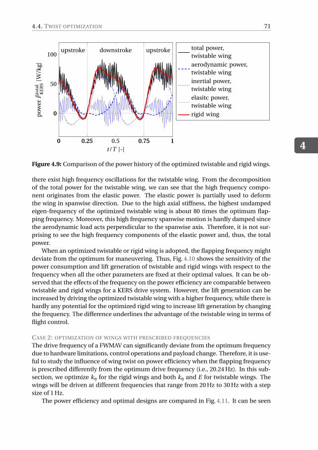
4.4. TWIST OPTIMIZATION
4
71
0 0.25 0.5 0.75 1
0
50
100
0 0.25 0.75 1
0
upstroke downstroke upstroke
t/T [-]
pow
erP
tota
lK
ER
S[W
/kg]
total power,twistable wing
aerodynamic power,twistable wing
inertial power,twistable wing
elasitc power,twistable wing
rigid wing
Figure 4.9: Comparison of the power history of the optimized twistable and rigid wings.
there exist high frequency oscillations for the twistable wing. From the decompositionof the total power for the twistable wing, we can see that the high frequency compo-nent originates from the elastic power. The elastic power is partially used to deformthe wing in spanwise direction. Due to the high axial stiffness, the highest undampedeigen-frequency of the optimized twistable wing is about 80 times the optimum flap-ping frequency. Moreover, this high frequency spanwise motion is hardly damped sincethe aerodynamic load acts perpendicular to the spanwise axis. Therefore, it is not sur-prising to see the high frequency components of the elastic power and, thus, the totalpower.
When an optimized twistable or rigid wing is adopted, the flapping frequency mightdeviate from the optimum for maneuvering. Thus, Fig. 4.10 shows the sensitivity of thepower consumption and lift generation of twistable and rigid wings with respect to thefrequency when all the other parameters are fixed at their optimal values. It can be ob-served that the effects of the frequency on the power efficiency are comparable betweentwistable and rigid wings for a KERS drive system. However, the lift generation can beincreased by driving the optimized twistable wing with a higher frequency, while there ishardly any potential for the optimized rigid wing to increase lift generation by changingthe frequency. The difference underlines the advantage of the twistable wing in terms offlight control.
CASE 2: OPTIMIZATION OF WINGS WITH PRESCRIBED FREQUENCIES
The drive frequency of a FWMAV can significantly deviate from the optimum frequencydue to hardware limitations, control operations and payload change. Therefore, it is use-ful to study the influence of wing twist on power efficiency when the flapping frequencyis prescribed differently from the optimum drive frequency (i.e., 20.24 Hz). In this sub-section, we optimize kη for the rigid wings and both kη and E for twistable wings. Thewings will be driven at different frequencies that range from 20 Hz to 30 Hz with a stepsize of 1 Hz.
The power efficiency and optimal designs are compared in Fig. 4.11. It can be seen
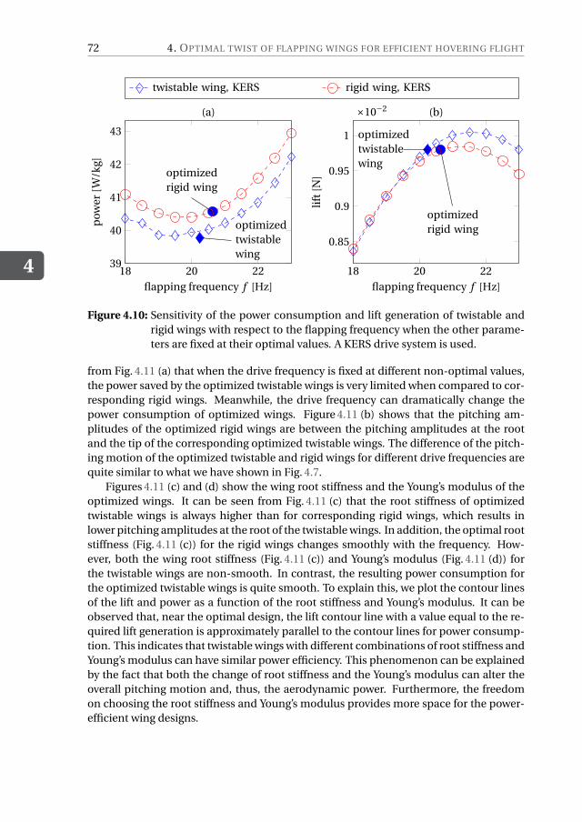
4
72 4. OPTIMAL TWIST OF FLAPPING WINGS FOR EFFICIENT HOVERING FLIGHT
18 20 2239
40
41
42
43
optimizedtwistablewing
optimizedrigid wing
flapping frequency f [Hz]
pow
er[W
/kg]
(a)
18 20 22
0.85
0.9
0.95
1
×10−2
optimizedtwistablewing
optimizedrigid wing
flapping frequency f [Hz]
lift
[N]
(b)
twistable wing, KERS rigid wing, KERS
Figure 4.10: Sensitivity of the power consumption and lift generation of twistable andrigid wings with respect to the flapping frequency when the other parame-ters are fixed at their optimal values. A KERS drive system is used.
from Fig. 4.11 (a) that when the drive frequency is fixed at different non-optimal values,the power saved by the optimized twistable wings is very limited when compared to cor-responding rigid wings. Meanwhile, the drive frequency can dramatically change thepower consumption of optimized wings. Figure 4.11 (b) shows that the pitching am-plitudes of the optimized rigid wings are between the pitching amplitudes at the rootand the tip of the corresponding optimized twistable wings. The difference of the pitch-ing motion of the optimized twistable and rigid wings for different drive frequencies arequite similar to what we have shown in Fig. 4.7.
Figures 4.11 (c) and (d) show the wing root stiffness and the Young’s modulus of theoptimized wings. It can be seen from Fig. 4.11 (c) that the root stiffness of optimizedtwistable wings is always higher than for corresponding rigid wings, which results inlower pitching amplitudes at the root of the twistable wings. In addition, the optimal rootstiffness (Fig. 4.11 (c)) for the rigid wings changes smoothly with the frequency. How-ever, both the wing root stiffness (Fig. 4.11 (c)) and Young’s modulus (Fig. 4.11 (d)) forthe twistable wings are non-smooth. In contrast, the resulting power consumption forthe optimized twistable wings is quite smooth. To explain this, we plot the contour linesof the lift and power as a function of the root stiffness and Young’s modulus. It can beobserved that, near the optimal design, the lift contour line with a value equal to the re-quired lift generation is approximately parallel to the contour lines for power consump-tion. This indicates that twistable wings with different combinations of root stiffness andYoung’s modulus can have similar power efficiency. This phenomenon can be explainedby the fact that both the change of root stiffness and the Young’s modulus can alter theoverall pitching motion and, thus, the aerodynamic power. Furthermore, the freedomon choosing the root stiffness and Young’s modulus provides more space for the power-efficient wing designs.
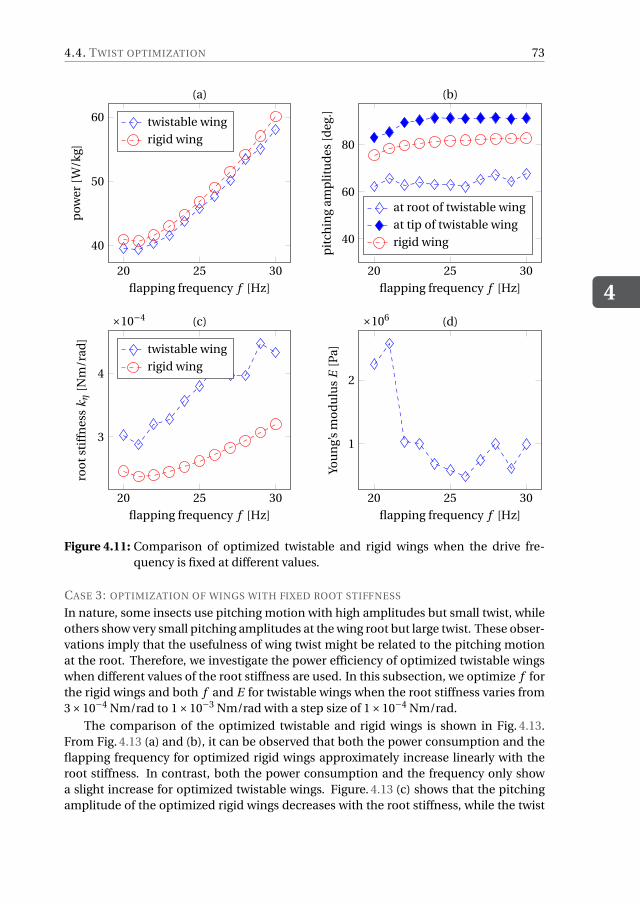
4.4. TWIST OPTIMIZATION
4
73
20 25 30
40
50
60
flapping frequency f [Hz]
pow
er[W
/kg]
(a)
twistable wing
rigid wing
20 25 30
40
60
80
flapping frequency f [Hz]
pit
chin
gam
pli
tud
es[d
eg.]
(b)
at root of twistable wing
at tip of twistable wing
rigid wing
20 25 30
3
4
×10−4
flapping frequency f [Hz]
roo
tsti
ffn
ess
kη
[Nm
/rad
]
(c)
twistable wing
rigid wing
20 25 30
1
2
×106
flapping frequency f [Hz]
You
ng’
sm
od
ulu
sE
[Pa]
(d)
Figure 4.11: Comparison of optimized twistable and rigid wings when the drive fre-quency is fixed at different values.
CASE 3: OPTIMIZATION OF WINGS WITH FIXED ROOT STIFFNESS
In nature, some insects use pitching motion with high amplitudes but small twist, whileothers show very small pitching amplitudes at the wing root but large twist. These obser-vations imply that the usefulness of wing twist might be related to the pitching motionat the root. Therefore, we investigate the power efficiency of optimized twistable wingswhen different values of the root stiffness are used. In this subsection, we optimize f forthe rigid wings and both f and E for twistable wings when the root stiffness varies from3×10−4 Nm/rad to 1×10⁻³ Nm/rad with a step size of 1×10⁻⁴ Nm/rad.
The comparison of the optimized twistable and rigid wings is shown in Fig. 4.13.From Fig. 4.13 (a) and (b), it can be observed that both the power consumption and theflapping frequency for optimized rigid wings approximately increase linearly with theroot stiffness. In contrast, both the power consumption and the frequency only showa slight increase for optimized twistable wings. Figure. 4.13 (c) shows that the pitchingamplitude of the optimized rigid wings decreases with the root stiffness, while the twist
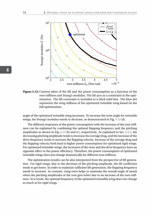
4
74 4. OPTIMAL TWIST OF FLAPPING WINGS FOR EFFICIENT HOVERING FLIGHT
55
50
50
45
45
40
40
40
3535
35
30
30
30
25
2520
15
optimum
2 2.5 3 3.5 4 4.5 5×10⁻⁴
105
106
107
root stiffness kη [Nm/rad]
You
ng’
sm
od
ulu
sE
[Pa]
ˆP totalKERS
L=1 g
Figure 4.12: Contour plots of the lift and the power consumption as a function of theroot stiffness and Young’s modulus. The lift acts as a constraint in the opti-mization. The lift constraint is included as a thick solid line. The blue dotrepresents the wing stiffness of the optimized twistable wing based on thefull optimization.
angle of the optimized twistable wing increases. To increase the twist angle for twistablewings, the Young’s modulus needs to decrease, as demonstrated in Fig. 4.13 (d).
The different responses of the power consumption with the increase of the root stiff-ness can be explained by combining the optimal flapping frequency and the pitchingamplitudes as shown in Fig. 4.13 (b) and (c), respectively. As explained in Sec. 4.4.2, thedecreasing pitching amplitude tends to increase the average drag, and the increase of thedrive frequency tends to increase the flapping velocity. Increase of the average drag andthe flapping velocity both lead to higher power consumption for optimized rigid wings.For optimized twistable wings, the increases of the twist and the drive frequency have anopposite effect to the power efficiency. Therefore, the power consumption of optimizedtwistable wings does not change dramatically for different root stiffness.
The optimization results can be also interpreted from the perspective of lift genera-tion. For rigid wings, due to the decrease of the pitching amplitude, the lift coefficienttends to get lower. In order to maintain sufficient lift generation, the flapping frequencyneeds to increase. In contrast, wing twist helps to maintain the overall angle of attackwhen the pitching amplitudes at the root gets lower due to an increase of the root stiff-ness. As a result, the optimal frequency of the optimized twistable wing does not changeas much as for rigid wings.
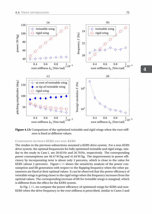
4.4. TWIST OPTIMIZATION
4
75
0.4 0.6 0.8 1×10⁻³
40
60
80
100
120
root stiffness kη [Nm/rad]
pow
er[W
/kg]
(a)
twistable wing
rigid wing
0.4 0.6 0.8 1×10⁻³
20
22
24
root stiffness kη [Nm/rad]
freq
uen
cyf
[Hz]
(b)
twistable wing
rigid wing
0.4 0.6 0.8 1×10⁻³
50
100
150
root stiffness kη [Nm/rad]
pit
chin
gam
pli
tud
es[d
eg.]
(c)
at root of twistable wing
at tip of twistable wing
rigid wing
0.4 0.6 0.8 1×10⁻³
105
106
root stiffness kη [Nm/rad]
You
ng’
sm
od
ulu
sE
[Pa]
(d)
Figure 4.13: Comparison of the optimized twistable and rigid wings when the root stiff-ness is fixed at different values.
COMPARISON BETWEEN KERS AND NON-KERSThe studies in the previous subsections assumed a KERS drive system. For a non-KERSdrive system, the optimal frequencies for fully optimized twistable and rigid wings, sim-ilar to the study in Case 1, are 20.65 Hz and 20.70 Hz, respectively. The correspondingpower consumptions are 40.47 W/kg and 41.64 W/kg. The improvement in power effi-ciency by incorporating twist is about only 3 percents, which is close to the value forKERS (about 2 percents). Figure 4.14 shows the sensitivity analysis of the power con-sumption and lift generation with respect to the flapping frequency when the other pa-rameters are fixed at their optimal values. It can be observed that the power efficiency oftwistable wings is getting closer to the rigid wings when the frequency increases from theoptimal values. The corresponding increase of lift for twistable wings is marginal, whichis different from the effect for the KERS system.
In Fig. 4.15, we compare the power efficiency of optimized wings for KERS and non-KERS when the drive frequency or the root stiffness is prescribed, similar to Cases 2 and
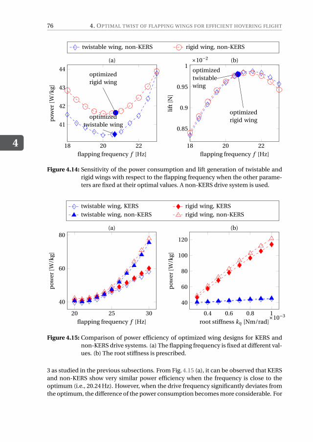
4
76 4. OPTIMAL TWIST OF FLAPPING WINGS FOR EFFICIENT HOVERING FLIGHT
18 20 22
41
42
43
44
optimizedtwistable wing
optimizedrigid wing
flapping frequency f [Hz]
pow
er[W
/kg]
(a)
18 20 22
0.85
0.9
0.95
1×10⁻²
optimizedtwistablewing
optimizedrigid wing
flapping frequency f [Hz]
lift
[N]
(b)
twistable wing, non-KERS rigid wing, non-KERS
Figure 4.14: Sensitivity of the power consumption and lift generation of twistable andrigid wings with respect to the flapping frequency when the other parame-ters are fixed at their optimal values. A non-KERS drive system is used.
20 25 30
40
60
80
flapping frequency f [Hz]
pow
er[W
/kg]
(a)
0.4 0.6 0.8 1×10⁻³
40
60
80
100
120
root stiffness kη [Nm/rad]
pow
er[W
/kg]
(b)
twistable wing, KERS rigid wing, KERS
twistable wing, non-KERS rigid wing, non-KERS
Figure 4.15: Comparison of power efficiency of optimized wing designs for KERS andnon-KERS drive systems. (a) The flapping frequency is fixed at different val-ues. (b) The root stiffness is prescribed.
3 as studied in the previous subsections. From Fig. 4.15 (a), it can be observed that KERSand non-KERS show very similar power efficiency when the frequency is close to theoptimum (i.e., 20.24 Hz). However, when the drive frequency significantly deviates fromthe optimum, the difference of the power consumption becomes more considerable. For
4.5. CONCLUSIONS
4
77
instance, when the frequency is fixed at 30 Hz, the optimized twistable wing can saveabout 23% of the power for KERS as compared to non-KERS. Figure 4.15 (b) shows that,for the optimized twistable wings, the power efficiency does not change significantlywith the prescribed root stiffness when a non-KERS system is used. This is similar tothe observation for KERS. Meanwhile, the difference between the power consumed forKERS and non-KERS are negligible for all the root stiffness. For optimized rigid wings,the difference between the power consumed by KERS and non-KERS slightly increaseswith the root stiffness but still not very pronounced.
4.5. CONCLUSIONSWe have proposed a computationally efficient Fluid-Structure Interaction (FSI) model toenable the parametric study and optimization of flapping wing twist and correspondingkinematics. The proposed FSI model relies on an analytical twist model and a quasi-steady aerodynamic model. The twist model uses a polynomial to describe the changeof the twist angle along the span. The spanwise shortening effect and the quadraticstrain-displacement relations for the wing membrane deformation have been includedto guarantee accuracy for large twist. It has been shown for rectangular wings that aquadratic polynomial can accurately model the twist at large amplitudes. Moreover, theproposed twist model and the quasi-steady aerodynamic model enable full FSI analysisin just a few minutes, which demonstrates the computational efficiency of the proposedFSI model.
Based on the proposed FSI model, we have optimized the stiffness and flapping fre-quency for both rigid and twistable wings to minimize the power consumption for hov-ering. Comparisons show that the optimized twistable wings exhibit power efficiencyclose to the optimized rigid wings, unless the pitching amplitude at the wing root is lim-ited. When the pitching amplitude at the root decreases by increasing the root stiffness,the optimized rigid wings need more power for hovering. However, the power efficien-cies of optimized twistable wings with different prescribed root stiffness are comparablewith the twistable wings with optimal root stiffness. This observation provides an expla-nation for the different levels of twist demonstrated by insect wings. The computationalefficiency of the proposed FSI model allows parametric study and optimization of flap-ping wings to enhance the understanding of insect wing flexibility and may help thedesign of flexible artificial wings for FWMAVs.

5ACTIVE ELASTIC WING HINGE
DESIGN BASED ON ELECTROSTATIC
STICKING
In previous chapters, we have shown that a proper root stiffness is essential for flappingwings to achieve optimal passive pitching motion. Since the required root stiffness changeswith the lift constraint, an elastic hinge with a tunable stiffness is helpful for a wing designto change its pitching motion when the required lift changes.
This chapter studies an elastic hinge design consisting of stacked layers which can besticked together using electrostatics. After the introduction, the passive pitching flappingmotion is described in Sec. 5.2. Next, the voltage-dependent behavior of this elastic hingeduring the large pitching motion is described in detail in Sec. 5.3. After that, the equa-tion of motion that governs the passive pitching motion is formulated as a function of thehinge stiffness and the applied control voltage (see Sec. 5.4). In Sec. 5.5, experiments areconducted to study the practical applicability of this method on FWMAVs. The experi-mental results are compared with the numerical simulations in Sec. 5.6. As concluded inSec. 5.7, the proposed hinge design is able to change the hinge stiffness, and it is a promis-ing approach for flapping wing flight control with refined fabrication techniques.
This chapter is based on the book chapter “Peters, H. J., Wang, Q., Goosen, J. F. L., & van Keulen, F., 2017. Activecontrol of the hinge of a flapping wing with electrostatic sticking to modify the passive pitching motion. In:A. L. Araujo and C. A. Mota Soares (Eds.), Smart Structures and Materials, Computational Methods in AppliedSciences 43, Springer International Publishing Switzerland.”
79
5
80 5. ACTIVE ELASTIC WING HINGE DESIGN BASED ON ELECTROSTATIC STICKING
5.1. INTRODUCTIONThe design and realization of lightweight Flapping Wing Micro Air Vehicles (FWMAVs)have attracted much attention over the last decades. Potential applications of FMWAVdesigns are in, among others, surveillance (e.g., police and security) and inspection ofinaccessible or dangerous locations (e.g., disaster scenes and sewers). The design andrealization of FWMAVs is complicated by weight constraints as a result of the limited liftproduction of the wings. Consequently, designers aim for lightweight, smart and highlyintegrated systems. This has resulted in several ways of achieving flapping kinematicsfor sufficient lift production. To decrease the actuation mechanism complexity, somewing designs integrate elastic hinges that allow the wing pitching motion to be passiveduring the flapping motion (Bolsman et al., 2009, Wood, 2008). Due to the inertial andaerodynamic loads, a properly tuned elastic hinge results in the required pitching mo-tion to achieve enough lift production to stay aloft.
For stable flight and maneuvering, FWMAV designs require some form of control.In fact, constant control will be necessary because of the intrinsic dynamic instabilityof the designs. Recent work on the Harvard Robobees (i.e., a FWMAV design whichexploits passive pitching) applied aerodynamic dampers for stabilization (Teoh et al.,2012), complex mechanisms to induce asymmetric flapping wing kinematics to pro-duce control torques (Finio & Wood, 2012), and separate actuators for each wing (Maet al., 2012). Additionally, control torques were created by integrating a piezoelectric bi-morph actuator in the wing elastic hinge to induce a bias during the wing stroke (Teoh& Wood, 2014). To control lightweight FWMAV designs, actively adjusting the dynamicproperties (i.e., structural damping and stiffness) of the wing elastic hinge appears to bea promising, elegant, and integrable approach to change the passive pitching motionduring flight and, hence, the stroke-averaged lift force. This control approach is not wellestablished within literature.
To actively change the dynamic properties of the wing elastic hinge, the hinge needsto be replaced by an active hinge which properties change due to some external stimuli(e.g., an electric field). Methods to actively change the dynamic properties of an elasticelement are, for example: (1) smart fluids (i.e., magnetorheological or electrorheologicalfluids) for which the properties transform rapidly upon exposure to an external mag-netic or electric field (Majidi & Wood, 2010), (2) piezoelectric polymer films (e.g., PVDF)for which the properties change as a function of the connected electrical circuit (Clark,2000), and (3) sticking stacked layers using, for example, electrostatics (Bergamini et al.,2006, Tabata et al., 2001).
This chapter investigates the method with the stacked layers for which the concep-tual idea is shown in Fig. 5.1. Figure 5.1(a) shows a capacitor-like clamped-free beamwhich consists of two layers which can slide with respect to each other when deflectedby the end-load F . Each layer consists of a conducting layer (e.g., spring steel) and a di-electric layer (e.g., Mylar). Figure 5.1(b) shows that, during deflection, the two layers slipwith respect to each other if the applied voltage V = 0. For a specific voltage Vst, the elec-trostatic loading causes the layers to stick to each other during deflection, see Fig. 5.1(c).Whenever these layers stick, the second moment of area increases, which effectively in-creases the bending stiffness of the beam.
This chapter aims to actively control the wing’s passive pitching motion by sticking
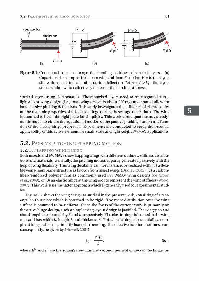
5.2. PASSIVE PITCHING FLAPPING MOTION
5
81
(a)
conductor
dieletric
F = 0(b)
F 6= 0
V = 0
(c)
F 6= 0
V Ê 0
Figure 5.1: Conceptual idea to change the bending stiffness of stacked layers. (a)Capacitor-like clamped-free beam with end-load F . (b) For V = 0, the layersslip with respect to each other during deflection. (c) For V Ê Vst, the layersstick together which effectively increases the bending stiffness.
stacked layers using electrostatics. These stacked layers need to be integrated into alightweight wing design (i.e., total wing design is about 200mg) and should allow forlarge passive pitching deflections. This study investigates the influence of electrostaticson the dynamic properties of this active hinge during these large deflections. The wingis assumed to be a thin, rigid plate for simplicity. This work uses a quasi-steady aerody-namic model to obtain the equation of motion of the passive pitching motion as a func-tion of the elastic hinge properties. Experiments are conducted to study the practicalapplicability of this active element for small-scale and lightweight FWMAV applications.
5.2. PASSIVE PITCHING FLAPPING MOTION
5.2.1. FLAPPING WING DESIGNBoth insects and FWMAVs show flapping wings with different outlines, stiffness distribu-tions and materials. Generally, the pitching motion is partly generated passively with thehelp of wing flexibility. This wing flexibility can, for instance, be realized with: (1) a flexi-ble veins-membrane structure as known from insect wings (Dudley, 2002), (2) a carbon-fiber-reinforced polymer film as commonly used in FWMAV wing designs (de Croonet al., 2009), or (3) an elastic hinge at the wing root to represent the wing stiffness (Wood,2007). This work uses the latter approach which is generally used for experimental stud-ies.
Figure 5.2 shows the wing design as studied in the present work, consisting of a rect-angular, thin plate which is assumed to be rigid. The mass distribution over the wingsurface is assumed to be uniform. Since the focus of the current work is primarily onthe active hinge design, such a simple wing layout design is justified. The wingspan andchord length are denoted by R and c, respectively. The elastic hinge is located at the wingroot and has width b, length L and thickness t . This elastic hinge is essentially a com-pliant hinge, which is primarily loaded in bending. The effective rotational stiffness can,consequently, be given by (Howell, 2001)
kη =E hI h
L, (5.1)
where E h and I h are the Young’s modulus and second moment of area of the hinge, re-
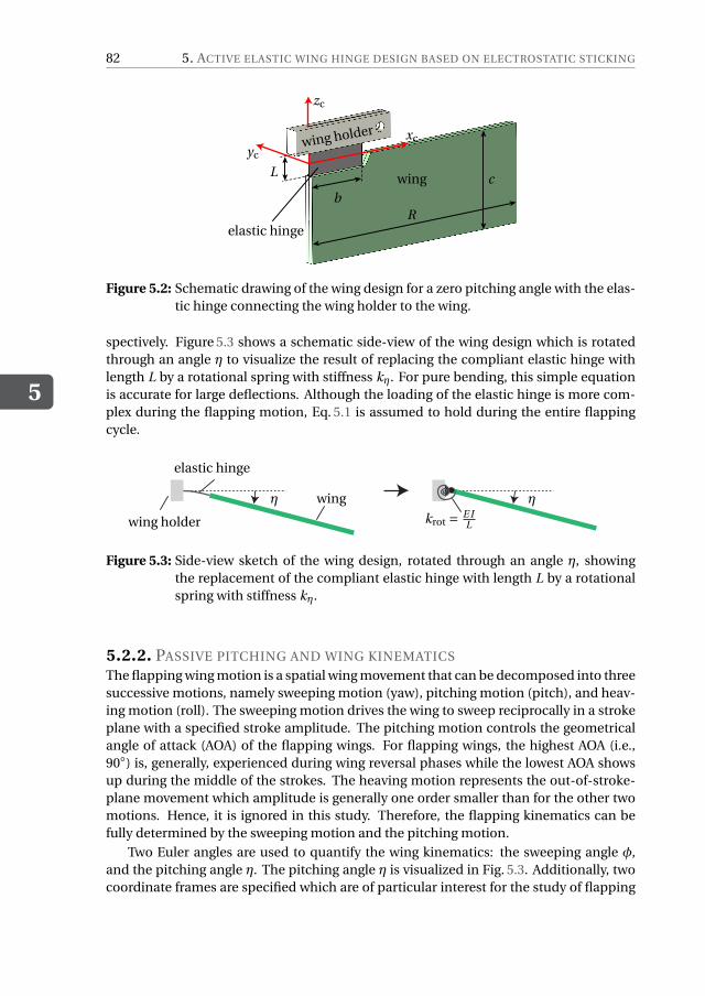
5
82 5. ACTIVE ELASTIC WING HINGE DESIGN BASED ON ELECTROSTATIC STICKING
elastic hinge
bR
cL
yc
xc
zc
wing holder
wing
Figure 5.2: Schematic drawing of the wing design for a zero pitching angle with the elas-tic hinge connecting the wing holder to the wing.
spectively. Figure 5.3 shows a schematic side-view of the wing design which is rotatedthrough an angle η to visualize the result of replacing the compliant elastic hinge withlength L by a rotational spring with stiffness kη. For pure bending, this simple equationis accurate for large deflections. Although the loading of the elastic hinge is more com-plex during the flapping motion, Eq. 5.1 is assumed to hold during the entire flappingcycle.
wing holder
elastic hinge
η wing
krot = E IL
η
Figure 5.3: Side-view sketch of the wing design, rotated through an angle η, showingthe replacement of the compliant elastic hinge with length L by a rotationalspring with stiffness kη.
5.2.2. PASSIVE PITCHING AND WING KINEMATICS
The flapping wing motion is a spatial wing movement that can be decomposed into threesuccessive motions, namely sweeping motion (yaw), pitching motion (pitch), and heav-ing motion (roll). The sweeping motion drives the wing to sweep reciprocally in a strokeplane with a specified stroke amplitude. The pitching motion controls the geometricalangle of attack (AOA) of the flapping wings. For flapping wings, the highest AOA (i.e.,90◦) is, generally, experienced during wing reversal phases while the lowest AOA showsup during the middle of the strokes. The heaving motion represents the out-of-stroke-plane movement which amplitude is generally one order smaller than for the other twomotions. Hence, it is ignored in this study. Therefore, the flapping kinematics can befully determined by the sweeping motion and the pitching motion.
Two Euler angles are used to quantify the wing kinematics: the sweeping angle φ,and the pitching angle η. The pitching angle η is visualized in Fig. 5.3. Additionally, twocoordinate frames are specified which are of particular interest for the study of flapping

5.3. ELECTROSTATICALLY CONTROLLED HINGE THEORY
5
83
wing motion: the fixed inertial frame xi yizi and the co-rotating frame xc yczc which co-rotates with the wing (see Fig. 5.2). The angular velocity and acceleration of a flappingwing in the co-rotating frame can be expressed by
ωc =[η, φsin(η), φcos(η)
]T(5.2)
andαc = ωc =
[η, φηcos(η)+ φsin(η), φcos(η)− φηsin(η)
]T, (5.3)
respectively. The AOA can be simply obtained by∣∣90◦−η
∣∣. The inertial and aerodynamicload can be fully determined if Eqs. 5.2 and 5.3 are known. For a given prescribed sweep-ing motion φ (t ), the tuned elastic hinge stiffness fully determines the (passive) pitchingmotion and, therefore, the aerodynamic load generation (e.g., lift force). Consequently,changing the elastic hinge stiffness in an active manner would lead to changes in theaerodynamic load generation and, hence, to a way to control FWMAV flight.
5.3. ELECTROSTATICALLY CONTROLLED HINGE THEORYThis section discusses a model to electrostatically control the dynamic properties of theactive hinge. First, it presents the proposed hinge design followed by a description of thevoltage-induced normal stress between the stacked layers. Subsequently, it describes thevoltage-dependent behavior during the flapping motion (i.e., whether the layers slip orstick). After that, the voltage-dependent properties of the active hinge (i.e., its rotationalstiffness and power dissipation) during the flapping motion are presented.
5.3.1. PROPOSED ELASTIC HINGE DESIGNThe elastic hinge in the wing design of Fig. 5.2 is replaced by an active hinge for which anenlarged side-view is shown in Fig. 5.4 (a). The hinge is symmetric in thickness direction.The hinge has length L and width b. It consists of a conducting core which is covered onboth sides by dielectric layers and two conducting facings. The core connects the wingholder to the wing while the two facings are attached to the wing holder only. The twofacings can slide with respect to the core. The thickness of the core, the dielectric layers,and the facings are denoted by tc, td, and tf, respectively (see Fig. 5.4 (b)). Two clamps areattached to the wing to prevent the layers from separating during the pitching motion.Hence, all layers will always contribute to the resulting bending stiffness. The facings areassumed to slip freely with respect to the clamps.
5.3.2. VOLTAGE-INDUCED STRESSES BETWEEN STACKED LAYERSBy applying a voltage V to the conducting facings of the active hinge while connectingthe conducting core to ground, an electric field is created over the dielectric layers, seeFig. 5.5 (a). This electric field induces a normal stress at the interface between the facingsand the dielectric layers, see Fig. 5.5 (b), which is given by (Bergamini et al., 2006)
σN (V ) = 1
2
ε0εrV 2
t 2d
, (5.4)
where ε0 represents the vacuum permittivity and εr is the material-dependent relativepermittivity. The normal stress depends quadratically on the applied voltage V and
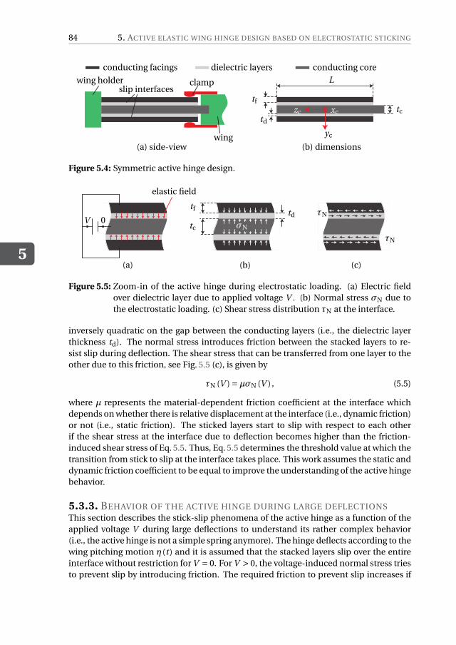
5
84 5. ACTIVE ELASTIC WING HINGE DESIGN BASED ON ELECTROSTATIC STICKING
wing holderslip interfaces
clamp
wing
conducting facings dielectric layers conducting core
tf
td
L
tc
yc
xczc
(a) side-view (b) dimensions
Figure 5.4: Symmetric active hinge design.
V 0
elastic field
tf
tc
td τN
τN
σN
(a) (b) (c)
Figure 5.5: Zoom-in of the active hinge during electrostatic loading. (a) Electric fieldover dielectric layer due to applied voltage V . (b) Normal stress σN due tothe electrostatic loading. (c) Shear stress distribution τN at the interface.
inversely quadratic on the gap between the conducting layers (i.e., the dielectric layerthickness td). The normal stress introduces friction between the stacked layers to re-sist slip during deflection. The shear stress that can be transferred from one layer to theother due to this friction, see Fig. 5.5 (c), is given by
τN (V ) =µσN (V ) , (5.5)
where µ represents the material-dependent friction coefficient at the interface whichdepends on whether there is relative displacement at the interface (i.e., dynamic friction)or not (i.e., static friction). The sticked layers start to slip with respect to each otherif the shear stress at the interface due to deflection becomes higher than the friction-induced shear stress of Eq. 5.5. Thus, Eq. 5.5 determines the threshold value at which thetransition from stick to slip at the interface takes place. This work assumes the static anddynamic friction coefficient to be equal to improve the understanding of the active hingebehavior.
5.3.3. BEHAVIOR OF THE ACTIVE HINGE DURING LARGE DEFLECTIONSThis section describes the stick-slip phenomena of the active hinge as a function of theapplied voltage V during large deflections to understand its rather complex behavior(i.e., the active hinge is not a simple spring anymore). The hinge deflects according to thewing pitching motion η (t ) and it is assumed that the stacked layers slip over the entireinterface without restriction for V = 0. For V > 0, the voltage-induced normal stress triesto prevent slip by introducing friction. The required friction to prevent slip increases if
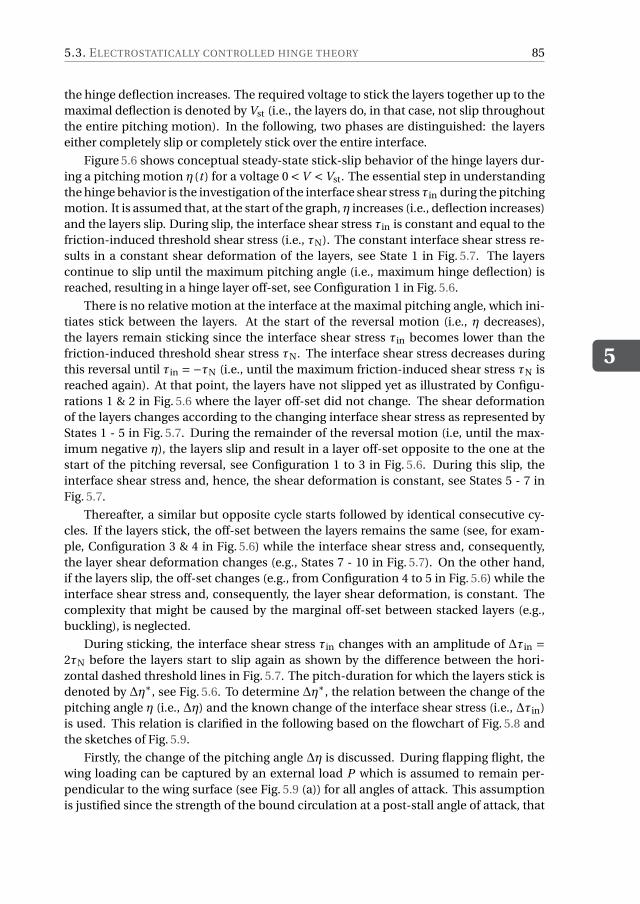
5.3. ELECTROSTATICALLY CONTROLLED HINGE THEORY
5
85
the hinge deflection increases. The required voltage to stick the layers together up to themaximal deflection is denoted by Vst (i.e., the layers do, in that case, not slip throughoutthe entire pitching motion). In the following, two phases are distinguished: the layerseither completely slip or completely stick over the entire interface.
Figure 5.6 shows conceptual steady-state stick-slip behavior of the hinge layers dur-ing a pitching motion η (t ) for a voltage 0 <V <Vst. The essential step in understandingthe hinge behavior is the investigation of the interface shear stress τin during the pitchingmotion. It is assumed that, at the start of the graph, η increases (i.e., deflection increases)and the layers slip. During slip, the interface shear stress τin is constant and equal to thefriction-induced threshold shear stress (i.e., τN). The constant interface shear stress re-sults in a constant shear deformation of the layers, see State 1 in Fig. 5.7. The layerscontinue to slip until the maximum pitching angle (i.e., maximum hinge deflection) isreached, resulting in a hinge layer off-set, see Configuration 1 in Fig. 5.6.
There is no relative motion at the interface at the maximal pitching angle, which ini-tiates stick between the layers. At the start of the reversal motion (i.e., η decreases),the layers remain sticking since the interface shear stress τin becomes lower than thefriction-induced threshold shear stress τN. The interface shear stress decreases duringthis reversal until τin = −τN (i.e., until the maximum friction-induced shear stress τN isreached again). At that point, the layers have not slipped yet as illustrated by Configu-rations 1 & 2 in Fig. 5.6 where the layer off-set did not change. The shear deformationof the layers changes according to the changing interface shear stress as represented byStates 1 - 5 in Fig. 5.7. During the remainder of the reversal motion (i.e, until the max-imum negative η), the layers slip and result in a layer off-set opposite to the one at thestart of the pitching reversal, see Configuration 1 to 3 in Fig. 5.6. During this slip, theinterface shear stress and, hence, the shear deformation is constant, see States 5 - 7 inFig. 5.7.
Thereafter, a similar but opposite cycle starts followed by identical consecutive cy-cles. If the layers stick, the off-set between the layers remains the same (see, for exam-ple, Configuration 3 & 4 in Fig. 5.6) while the interface shear stress and, consequently,the layer shear deformation changes (e.g., States 7 - 10 in Fig. 5.7). On the other hand,if the layers slip, the off-set changes (e.g., from Configuration 4 to 5 in Fig. 5.6) while theinterface shear stress and, consequently, the layer shear deformation, is constant. Thecomplexity that might be caused by the marginal off-set between stacked layers (e.g.,buckling), is neglected.
During sticking, the interface shear stress τin changes with an amplitude of ∆τin =2τN before the layers start to slip again as shown by the difference between the hori-zontal dashed threshold lines in Fig. 5.7. The pitch-duration for which the layers stick isdenoted by ∆η∗, see Fig. 5.6. To determine ∆η∗, the relation between the change of thepitching angle η (i.e., ∆η) and the known change of the interface shear stress (i.e., ∆τin)is used. This relation is clarified in the following based on the flowchart of Fig. 5.8 andthe sketches of Fig. 5.9.
Firstly, the change of the pitching angle ∆η is discussed. During flapping flight, thewing loading can be captured by an external load P which is assumed to remain per-pendicular to the wing surface (see Fig. 5.9 (a)) for all angles of attack. This assumptionis justified since the strength of the bound circulation at a post-stall angle of attack, that
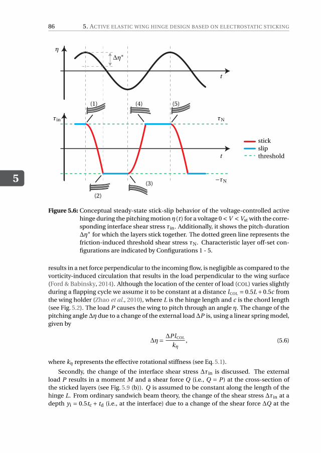
5
86 5. ACTIVE ELASTIC WING HINGE DESIGN BASED ON ELECTROSTATIC STICKING
η
τin
∆η∗
t
t
τN
−τN
(1)
(2)
(3)
(4) (5)
stickslipthreshold
Figure 5.6: Conceptual steady-state stick-slip behavior of the voltage-controlled activehinge during the pitching motion η (t ) for a voltage 0 <V <Vst with the corre-sponding interface shear stress τin. Additionally, it shows the pitch-duration∆η∗ for which the layers stick together. The dotted green line represents thefriction-induced threshold shear stress τN. Characteristic layer off-set con-figurations are indicated by Configurations 1 - 5.
results in a net force perpendicular to the incoming flow, is negligible as compared to thevorticity-induced circulation that results in the load perpendicular to the wing surface(Ford & Babinsky, 2014). Although the location of the center of load (COL) varies slightlyduring a flapping cycle we assume it to be constant at a distance lCOL = 0.5L +0.5c fromthe wing holder (Zhao et al., 2010), where L is the hinge length and c is the chord length(see Fig. 5.2). The load P causes the wing to pitch through an angle η. The change of thepitching angle∆η due to a change of the external load∆P is, using a linear spring model,given by
∆η= ∆PlCOL
kη, (5.6)
where kη represents the effective rotational stiffness (see Eq. 5.1).
Secondly, the change of the interface shear stress ∆τin is discussed. The externalload P results in a moment M and a shear force Q (i.e., Q = P ) at the cross-section ofthe sticked layers (see Fig. 5.9 (b)). Q is assumed to be constant along the length of thehinge L. From ordinary sandwich beam theory, the change of the shear stress ∆τin at adepth yi = 0.5tc + td (i.e., at the interface) due to a change of the shear force ∆Q at the
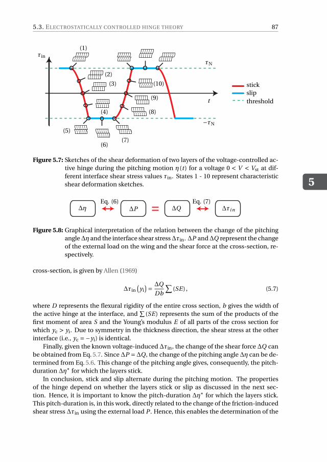
5.3. ELECTROSTATICALLY CONTROLLED HINGE THEORY
5
87
τin
t
τN
−τN
(1)
(2)
(3)
(4)
(5)
(6)(7)
(8)
(9)
(10) stickslipthreshold
Figure 5.7: Sketches of the shear deformation of two layers of the voltage-controlled ac-tive hinge during the pitching motion η (t ) for a voltage 0 < V < Vst at dif-ferent interface shear stress values τin. States 1 - 10 represent characteristicshear deformation sketches.
∆η ∆P ∆Q ∆τi n
Eq. (6) Eq. (7)
Figure 5.8: Graphical interpretation of the relation between the change of the pitchingangle∆η and the interface shear stress∆τin. ∆P and∆Q represent the changeof the external load on the wing and the shear force at the cross-section, re-spectively.
cross-section, is given by Allen (1969)
∆τin(yi
)= ∆Q
Db
∑(SE) , (5.7)
where D represents the flexural rigidity of the entire cross section, b gives the width ofthe active hinge at the interface, and
∑(SE) represents the sum of the products of the
first moment of area S and the Young’s modulus E of all parts of the cross section forwhich yc > yi. Due to symmetry in the thickness direction, the shear stress at the otherinterface (i.e., yc =−yi) is identical.
Finally, given the known voltage-induced ∆τin, the change of the shear force ∆Q canbe obtained from Eq. 5.7. Since∆P =∆Q, the change of the pitching angle∆η can be de-termined from Eq. 5.6. This change of the pitching angle gives, consequently, the pitch-duration ∆η∗ for which the layers stick.
In conclusion, stick and slip alternate during the pitching motion. The propertiesof the hinge depend on whether the layers stick or slip as discussed in the next sec-tion. Hence, it is important to know the pitch-duration ∆η∗ for which the layers stick.This pitch-duration is, in this work, directly related to the change of the friction-inducedshear stress ∆τin using the external load P . Hence, this enables the determination of the
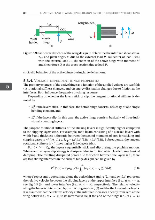
5
88 5. ACTIVE ELASTIC WING HINGE DESIGN BASED ON ELECTROSTATIC STICKING
wingholder
elastichinge P
lCOL
COL
wing
wing holder
yc
yi Q M
(a) (b)
Figure 5.9: Side-view sketches of the wing design to determine the interface shear stress,τin, and pitch angle, η, due to the external load P . (a) center of load (COL)with the external load P . (b) zoom-in of the active hinge with moment Mand shear force Q at the cross-section due to load P .
stick-slip behavior of the active hinge during large deflections.
5.3.4. VOLTAGE-DEPENDENT HINGE PROPERTIESThe property changes of the active hinge as a function of the applied voltage are twofold:(1) rotational stiffness changes, and (2) energy dissipation changes due to friction at theinterfaces. Both influence the passive pitching response.
Depending on whether the layers stick or slip, the tangent rotational stiffness is de-noted by
• kstη if the layers stick. In this case, the active hinge consists, basically, of one single
bending element, and
• kslη if the layers slip. In this case, the active hinge consists, basically, of three indi-
vidually bending layers.
The tangent rotational stiffness of the sticking layers is significantly higher comparedto the slipping layers case. For example, for a beam consisting of n stacked layers withwidth b and thickness t , the ratio between the second moments of area for sticking andslipping cases is n2 (i.e., Istick/Islip = (n3bh3/12)/(nbh3/12)). Subsequently, the tangentrotational stiffness is n2 times higher if the layers stick.
For 0 < V < Vst, the layers sequentially stick and slip during the pitching motion.Whenever the layers slip, energy is dissipated due to friction which leads to mechanicaldamping. The resulting dissipated power due to friction between the layers (i.e., thereare two sliding interfaces in the current hinge design) can be given by
P fr (V , t ) =µdσN (V )b∫ L
0(v1 (ξ, t )+ v2 (ξ, t ))dξ, (5.8)
where ξ represents a coordinate along the active hinge and v1 (ξ, t ) and v2 (ξ, t ) representthe relative velocity between the slipping layers at the upper interface (i.e., at yc = −yi,see Fig. 5.9 (b)) and lower interface (i.e., at yc = yi), respectively. The relative velocityalong the hinge is determined by the pitching motion η (t ) and the thickness of the layers.It is assumed that the relative velocity at the interface increases linearly from zero at thewing holder (i.e., at ξ = 0) to its maximal value at the end of the hinge (i.e., at ξ = L)
5.4. EQUATION OF MOTION OF PASSIVE PITCHING MOTION
5
89
although the velocity distribution might be more complex in reality. During slip, thecounteracting moment due to the friction can, subsequently, be obtained by
M frxc
={
0 for V = 0,P fr (V , t )/η for V 6= 0.
(5.9)
Equation 5.9 explicitly assumes that the dissipated power is equal to zero for V = 0 al-though this assumption oversimplifies the occurring slip behavior due to the inevitablenormal stress between slipping layers which are jointly bending. This description allows,despite the limitations, to study the influence of an electrostatically controlled activehinge on the passive pitching motion of a flapping wing.
5.4. EQUATION OF MOTION OF PASSIVE PITCHING MOTION
Since the sweeping motion φ (t ) is prescribed, the rigid wing model involves only onedegree of freedom, the pitching angle η. The equation of motion that governs η can beobtained by applying Euler’s second law of motion. That is,
M appliedxc
+M inerxc
= 0, (5.10)
where the inertial torque, M inerxc
, in the co-rotating frame is given by
M inerxc
= Ixcxc
[1
2sin(2η)φ2 − η
]− Ixczc φcos(η), (5.11)
where Ixcxc and Ixczc are moment of inertia terms. The applied torque, M appliedxc
, actingaround the pitching axis consists of three components: (1) the elastic torque from theactive hinge, M elas
xc, (2) the voltage-dependent torque due to the friction between the
layers, M frxc
, as calculated by Eq. 5.9, and (3) the aerodynamic torque M aeroxc
.
A quasi-steady aerodynamic model is used to calculate the transient aerodynamicloads. This chapter only shows the terms relevant for this work without going into muchdetail on the specific terms. For more details the reader is referred to Wang et al. (2016).The aerodynamic model assumes the resultant aerodynamic load acting on the wing tobe always perpendicular to the chord over the entire stroke (i.e., in yc-direction). For thinplates, this assumption is justified due to a negligible leading-edge suction load and wingsurface viscous drag compared to the dominant pressure load. The loads are decom-posed into four components which originate from different sources: (1) from the wingtranslational velocity, leading to F trans
ycand M trans
yc(Sane & Dickinson, 2002), (2) from the
coupling effect between wing translational and rotational effect, leading to F couplyc
and
M couplyc
, (3) from the pure rotational velocity, leading to F rotyc
and M rotyc
, and (4) from theadded mass effect, leading to F am
ycand M am
yc(Newman, 1977). The resultant aerodynamic

5
90 5. ACTIVE ELASTIC WING HINGE DESIGN BASED ON ELECTROSTATIC STICKING
loads can be calculated by
F aeroyc
= −sgn(ωzc )1
6ρfcR3cF trans
yc(ω2
yc+ω2
zc)
︸ ︷︷ ︸F trans
yc
+ 3
8πρfc
2R2ωxcωyc
︸ ︷︷ ︸F coupl
yc
−1
6ρfc
3RC rotωxc |ωxc |︸ ︷︷ ︸
F rotyc
+ π
8ρfc
2R[−R(αzc +ωxcωyc )− cαxc
]
︸ ︷︷ ︸F am
yc
(5.12)
and
M aeroyc
= −sgn(ωzc )1
6ρfc
2R3cF transyc
ztranscp (ω2
yc+ω2
zc)
︸ ︷︷ ︸M trans
yc
+ 3
32πρfc
3R2ωxcωyc
︸ ︷︷ ︸M coupl
yc
− 1
8ρfc
4RC rotωxc |ωxc |︸ ︷︷ ︸
M rotyc
+ π
16ρfc
3R
[−R(αzc +ωxcωyc )− 9
8cαxc
]
︸ ︷︷ ︸M am
yc
(5.13)
respectively, where ρf is the density of the fluid, ztranscp is the position of the center of
pressure due to the translational force which is calculated using an empirical formula(i.e., ztrans
cp = 0.261(AOA)+0.05), and C rot is the drag coefficient for a plate revolving at anAOA of 90◦. An analytical model proposed by Taha et al. (2014) is used to calculate the liftcoefficient cF trans
ycdue to the wing translational velocity. This analytical formula provides
a good prediction of the lift coefficients of translational flapping wings with differentaspect ratios according to the comparison with experimental data from bumble bees,fruit flies and hawk moths.
Eventually, the voltage-dependent equation of motion of the wing passive pitchingcan be expressed as
Ixcxc η+kηη= M aeroyc
+ f (η, η)+M frxc
(η,V
), (5.14)
where the inertial drive torque f (η, η) is given by
f (η, η) = 1
2Ixcxc φ
2 sin(2η)− Ixczc φcos(η). (5.15)
Finally, Eq. 5.13 will be used to determine the average lift generated by the flapping wingwith the actively controlled elastic hinge. It should be mentioned that the introducedquasi-steady model cannot capture some unsteady effects (e.g., wake capture effect andWagner effect). Rather good agreements can, however, be found between the resultsfrom the quasi-steady model and experiments (Wang et al., 2016) since the most impor-tant unsteady effect (i.e., the prolonged attached of the leading edge vortex) is captured.As such, the model is adequate for this work.
5.5. EXPERIMENTAL ANALYSISTo validate the presented approach on changing the dynamic properties of wing hinges,experiments are done. First, the manufactured wing equipped with an active hinge is
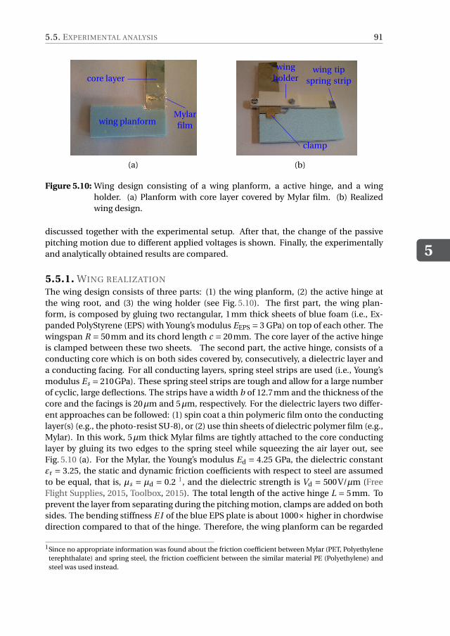
5.5. EXPERIMENTAL ANALYSIS
5
91
core layer
Mylarfilmwing planform
(a)
wingholder
wing tipspring strip
clamp
(b)
Figure 5.10: Wing design consisting of a wing planform, a active hinge, and a wingholder. (a) Planform with core layer covered by Mylar film. (b) Realizedwing design.
discussed together with the experimental setup. After that, the change of the passivepitching motion due to different applied voltages is shown. Finally, the experimentallyand analytically obtained results are compared.
5.5.1. WING REALIZATION
The wing design consists of three parts: (1) the wing planform, (2) the active hinge atthe wing root, and (3) the wing holder (see Fig. 5.10). The first part, the wing plan-form, is composed by gluing two rectangular, 1mm thick sheets of blue foam (i.e., Ex-panded PolyStyrene (EPS) with Young’s modulus EEPS = 3 GPa) on top of each other. Thewingspan R = 50mm and its chord length c = 20mm. The core layer of the active hingeis clamped between these two sheets. The second part, the active hinge, consists of aconducting core which is on both sides covered by, consecutively, a dielectric layer anda conducting facing. For all conducting layers, spring steel strips are used (i.e., Young’smodulus Es = 210GPa). These spring steel strips are tough and allow for a large numberof cyclic, large deflections. The strips have a width b of 12.7mm and the thickness of thecore and the facings is 20µm and 5µm, respectively. For the dielectric layers two differ-ent approaches can be followed: (1) spin coat a thin polymeric film onto the conductinglayer(s) (e.g., the photo-resist SU-8), or (2) use thin sheets of dielectric polymer film (e.g.,Mylar). In this work, 5µm thick Mylar films are tightly attached to the core conductinglayer by gluing its two edges to the spring steel while squeezing the air layer out, seeFig. 5.10 (a). For the Mylar, the Young’s modulus Ed = 4.25 GPa, the dielectric constantεr = 3.25, the static and dynamic friction coefficients with respect to steel are assumedto be equal, that is, µs = µd = 0.2 1, and the dielectric strength is Vd = 500V/µm (FreeFlight Supplies, 2015, Toolbox, 2015). The total length of the active hinge L = 5mm. Toprevent the layer from separating during the pitching motion, clamps are added on bothsides. The bending stiffness E I of the blue EPS plate is about 1000× higher in chordwisedirection compared to that of the hinge. Therefore, the wing planform can be regarded
1Since no appropriate information was found about the friction coefficient between Mylar (PET, Polyethyleneterephthalate) and spring steel, the friction coefficient between the similar material PE (Polyethylene) andsteel was used instead.
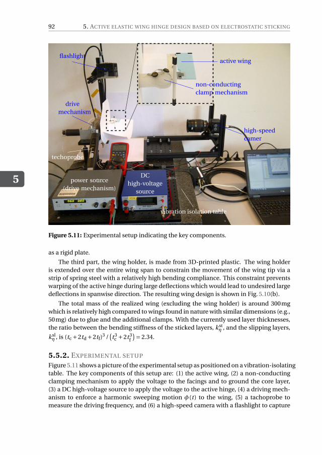
5
92 5. ACTIVE ELASTIC WING HINGE DESIGN BASED ON ELECTROSTATIC STICKING
flashlight
drivemechanism
techoprobe
power source(drive mechanism)
DChigh-voltage
source
vibration isolation table
high-speedcamer
non-conductingclamp mechanism
active wing
Figure 5.11: Experimental setup indicating the key components.
as a rigid plate.
The third part, the wing holder, is made from 3D-printed plastic. The wing holderis extended over the entire wing span to constrain the movement of the wing tip via astrip of spring steel with a relatively high bending compliance. This constraint preventswarping of the active hinge during large deflections which would lead to undesired largedeflections in spanwise direction. The resulting wing design is shown in Fig. 5.10(b).
The total mass of the realized wing (excluding the wing holder) is around 300mgwhich is relatively high compared to wings found in nature with similar dimensions (e.g.,50mg) due to glue and the additional clamps. With the currently used layer thicknesses,the ratio between the bending stiffness of the sticked layers, kst
η , and the slipping layers,
kslη , is (tc +2td +2tf)
3 /(t 3
c +2t 3f
)= 2.34.
5.5.2. EXPERIMENTAL SETUP
Figure 5.11 shows a picture of the experimental setup as positioned on a vibration-isolatingtable. The key components of this setup are: (1) the active wing, (2) a non-conductingclamping mechanism to apply the voltage to the facings and to ground the core layer,(3) a DC high-voltage source to apply the voltage to the active hinge, (4) a driving mech-anism to enforce a harmonic sweeping motion φ (t ) to the wing, (5) a tachoprobe tomeasure the driving frequency, and (6) a high-speed camera with a flashlight to capture
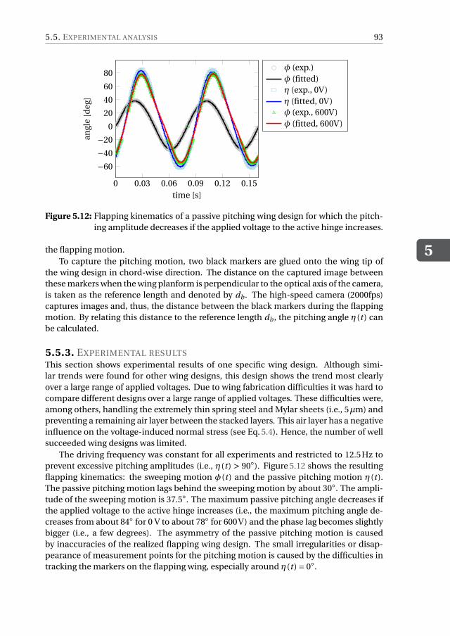
5.5. EXPERIMENTAL ANALYSIS
5
93
0 0.03 0.06 0.09 0.12 0.15
−60
−40
−20
0
20
40
60
80
time [s]
angl
e[d
eg]
φ (exp.)φ (fitted)η (exp., 0V)η (fitted, 0V)φ (exp., 600V)φ (fitted, 600V)
Figure 5.12: Flapping kinematics of a passive pitching wing design for which the pitch-ing amplitude decreases if the applied voltage to the active hinge increases.
the flapping motion.To capture the pitching motion, two black markers are glued onto the wing tip of
the wing design in chord-wise direction. The distance on the captured image betweenthese markers when the wing planform is perpendicular to the optical axis of the camera,is taken as the reference length and denoted by db . The high-speed camera (2000fps)captures images and, thus, the distance between the black markers during the flappingmotion. By relating this distance to the reference length db , the pitching angle η (t ) canbe calculated.
5.5.3. EXPERIMENTAL RESULTSThis section shows experimental results of one specific wing design. Although simi-lar trends were found for other wing designs, this design shows the trend most clearlyover a large range of applied voltages. Due to wing fabrication difficulties it was hard tocompare different designs over a large range of applied voltages. These difficulties were,among others, handling the extremely thin spring steel and Mylar sheets (i.e., 5µm) andpreventing a remaining air layer between the stacked layers. This air layer has a negativeinfluence on the voltage-induced normal stress (see Eq. 5.4). Hence, the number of wellsucceeded wing designs was limited.
The driving frequency was constant for all experiments and restricted to 12.5Hz toprevent excessive pitching amplitudes (i.e., η (t ) > 90◦). Figure 5.12 shows the resultingflapping kinematics: the sweeping motion φ (t ) and the passive pitching motion η (t ).The passive pitching motion lags behind the sweeping motion by about 30◦. The ampli-tude of the sweeping motion is 37.5◦. The maximum passive pitching angle decreases ifthe applied voltage to the active hinge increases (i.e., the maximum pitching angle de-creases from about 84◦ for 0 V to about 78◦ for 600V) and the phase lag becomes slightlybigger (i.e., a few degrees). The asymmetry of the passive pitching motion is causedby inaccuracies of the realized flapping wing design. The small irregularities or disap-pearance of measurement points for the pitching motion is caused by the difficulties intracking the markers on the flapping wing, especially around η (t ) = 0◦.
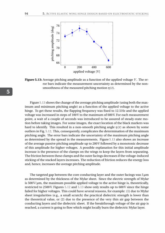
5
94 5. ACTIVE ELASTIC WING HINGE DESIGN BASED ON ELECTROSTATIC STICKING
0 200 400 60066
68
70
72
74
76
applied voltage [V]
pit
chin
gam
pli
tud
e[d
eg]
Figure 5.13: Average pitching amplitude as a function of the applied voltage V . The er-ror bars indicate the measurement uncertainty as determined by the non-smoothness of the measured pitching motion η (t ).
Figure 5.13 shows the change of the average pitching amplitude (using both the max-imum and minimum pitching angle) as a function of the applied voltage to the activehinge. To get these results, the flapping frequency was fixed to 12.5Hz and the appliedvoltage was increased in steps of 100V to the maximum of 600V. For each measurementpoint, a wait of a couple of seconds was introduced to be assured of steady-state mo-tion before taking images. For some images, the exact location of the black markers washard to identify. This resulted in a non-smooth pitching angle η (t ) as shown by someoutliers in Fig. 5.12. This, consequently, complicates the determination of the maximumpitching angle. The error bars indicate the uncertainty of the maximum pitching angleas determined by the spread in the measurements. Figure 5.13 also shows an increaseof the average passive pitching amplitude up to 200V followed by a monotonic decreaseof this amplitude for higher voltages. A possible explanation for this initial amplitudeincrease is the presence of the clamps on the wings to keep the layers from separating.The friction between these clamps and the outer facings decreases if the voltage-inducedsticking of the stacked layers increases. The reduction of friction reduces the energy lossand, hence, increases the average pitching amplitude.
The targeted gap between the core conducting layer and the outer facings was 5µmas determined by the thickness of the Mylar sheet. Since the electric strength of Mylaris 500V/µm, the maximum possible applied voltage to the active hinge is, theoretically,restricted to 2500V. Figures 5.12 and 5.13 show only results up to 600V since the hingefailed for higher voltages. This could have several reasons, for example: (1) due to Mylarsheet irregularities (e.g., a small scratch) the practical dielectric strength is lower thanthe theoretical value, or (2) due to the presence of the very thin air gap between theconducting layers and the dielectric sheet. If the breakthrough voltage of the air gap isreached, a current is going to flow which might locally burn the dielectric Mylar layer.
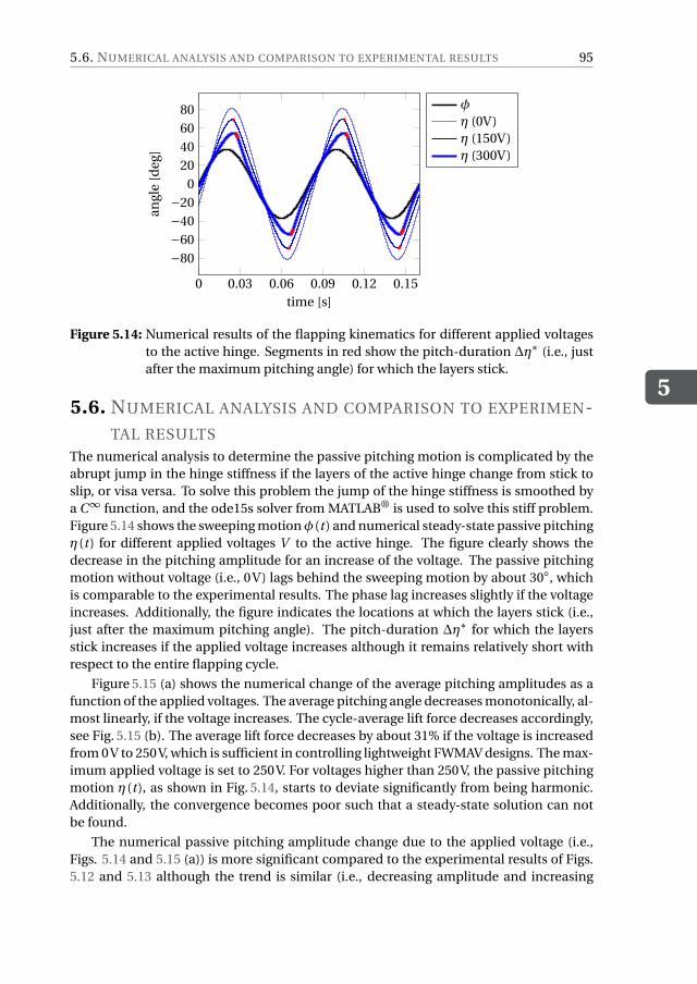
5.6. NUMERICAL ANALYSIS AND COMPARISON TO EXPERIMENTAL RESULTS
5
95
0 0.03 0.06 0.09 0.12 0.15
−80−60−40−20
020406080
time [s]
angl
e[d
eg]
φ
η (0V)η (150V)η (300V)
Figure 5.14: Numerical results of the flapping kinematics for different applied voltagesto the active hinge. Segments in red show the pitch-duration ∆η∗ (i.e., justafter the maximum pitching angle) for which the layers stick.
5.6. NUMERICAL ANALYSIS AND COMPARISON TO EXPERIMEN-TAL RESULTS
The numerical analysis to determine the passive pitching motion is complicated by theabrupt jump in the hinge stiffness if the layers of the active hinge change from stick toslip, or visa versa. To solve this problem the jump of the hinge stiffness is smoothed bya C∞ function, and the ode15s solver from MATLAB® is used to solve this stiff problem.Figure 5.14 shows the sweeping motionφ (t ) and numerical steady-state passive pitchingη (t ) for different applied voltages V to the active hinge. The figure clearly shows thedecrease in the pitching amplitude for an increase of the voltage. The passive pitchingmotion without voltage (i.e., 0V) lags behind the sweeping motion by about 30◦, whichis comparable to the experimental results. The phase lag increases slightly if the voltageincreases. Additionally, the figure indicates the locations at which the layers stick (i.e.,just after the maximum pitching angle). The pitch-duration ∆η∗ for which the layersstick increases if the applied voltage increases although it remains relatively short withrespect to the entire flapping cycle.
Figure 5.15 (a) shows the numerical change of the average pitching amplitudes as afunction of the applied voltages. The average pitching angle decreases monotonically, al-most linearly, if the voltage increases. The cycle-average lift force decreases accordingly,see Fig. 5.15 (b). The average lift force decreases by about 31% if the voltage is increasedfrom 0V to 250V, which is sufficient in controlling lightweight FWMAV designs. The max-imum applied voltage is set to 250V. For voltages higher than 250V, the passive pitchingmotion η (t ), as shown in Fig. 5.14, starts to deviate significantly from being harmonic.Additionally, the convergence becomes poor such that a steady-state solution can notbe found.
The numerical passive pitching amplitude change due to the applied voltage (i.e.,Figs. 5.14 and 5.15 (a)) is more significant compared to the experimental results of Figs.5.12 and 5.13 although the trend is similar (i.e., decreasing amplitude and increasing
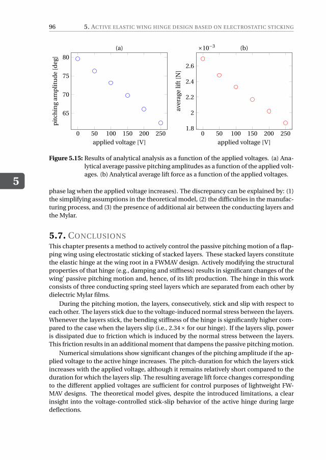
5
96 5. ACTIVE ELASTIC WING HINGE DESIGN BASED ON ELECTROSTATIC STICKING
0 50 100 150 200 250
65
70
75
80
applied voltage [V]
pit
chin
gam
pli
tud
e[d
eg]
(a)
0 50 100 150 200 2501.8
2
2.2
2.4
2.6
×10−3
applied voltage [V]
aver
age
lift[
N]
(b)
Figure 5.15: Results of analytical analysis as a function of the applied voltages. (a) Ana-lytical average passive pitching amplitudes as a function of the applied volt-ages. (b) Analytical average lift force as a function of the applied voltages.
phase lag when the applied voltage increases). The discrepancy can be explained by: (1)the simplifying assumptions in the theoretical model, (2) the difficulties in the manufac-turing process, and (3) the presence of additional air between the conducting layers andthe Mylar.
5.7. CONCLUSIONSThis chapter presents a method to actively control the passive pitching motion of a flap-ping wing using electrostatic sticking of stacked layers. These stacked layers constitutethe elastic hinge at the wing root in a FWMAV design. Actively modifying the structuralproperties of that hinge (e.g., damping and stiffness) results in significant changes of thewing’ passive pitching motion and, hence, of its lift production. The hinge in this workconsists of three conducting spring steel layers which are separated from each other bydielectric Mylar films.
During the pitching motion, the layers, consecutively, stick and slip with respect toeach other. The layers stick due to the voltage-induced normal stress between the layers.Whenever the layers stick, the bending stiffness of the hinge is significantly higher com-pared to the case when the layers slip (i.e., 2.34× for our hinge). If the layers slip, poweris dissipated due to friction which is induced by the normal stress between the layers.This friction results in an additional moment that dampens the passive pitching motion.
Numerical simulations show significant changes of the pitching amplitude if the ap-plied voltage to the active hinge increases. The pitch-duration for which the layers stickincreases with the applied voltage, although it remains relatively short compared to theduration for which the layers slip. The resulting average lift force changes correspondingto the different applied voltages are sufficient for control purposes of lightweight FW-MAV designs. The theoretical model gives, despite the introduced limitations, a clearinsight into the voltage-controlled stick-slip behavior of the active hinge during largedeflections.

5.7. CONCLUSIONS
5
97
Experiments are conducted to study the practical applicability of this active elastichinge for small-scale and lightweight FWMAV applications. To obtain experimental re-sults, several fabrication difficulties have been tackled, for example, the handling of thevery thin Mylar films (i.e., 5µm). The experimental results show, although suppressed,the same trends compared to the numerical simulations. The results are less significant,mainly due to: (1) the presence of an air layer between the conducting layers and thedielectric layers, (2) the presence of Mylar film irregularities. Despite of these shortcom-ings, the results clearly show a decrease of the pitching amplitude as a function of theapplied voltage. Hence, it shows the potential of this method to control FWMAVs.
In future work, the numerical model might be improved to model the stick-slip be-havior of the active hinge more accurately (e.g., the friction between the layers in the ab-sence of a control voltage). Additionally, long lasting experiments need to be conductedto study the influence of wear due to friction between the Mylar and the conductingsheets. Alternatively, it is interesting to change the applied voltage during a flapping cy-cle and study the occurring transient behavior. The fabrication process can be optimizedby preparing jigs or well-designed tools.


6RETROSPECTION AND DISCUSSION
Chapters 2 - 5 presented the modeling, design and optimization of flapping wings for ef-ficient hovering flight from different perspectives. In this chapter, these work are retro-spected from a bird’s-eye view, and the highlights and pitfalls of new designs are discussed.Preliminary investigations on other aspects of flapping wings are also introduced. At theend, the techniques and approaches we have used for wing fabrication and measurementare presented.
99
6
100 6. RETROSPECTION AND DISCUSSION
6.1. FLAPPING WING MODELINGFrom Chapter 2 to Chapter 5, flapping wings were modeled from different aspects, in-cluding the morphology, kinematics, flexibility, aerodynamics, aeroelasticity and thepower consumption. These models played an important role in the design of energy-efficient flapping wings.
6.1.1. MORPHOLOGYIn order to design and optimize flapping wings, the shape and mass distribution wereparameterized. From the work of Ellington (1984a), we know that the spanwise areadistribution of insect wings can be approximately quantified by a single parameter rs1 ,which represents the spanwise distance between the root and the centroid. Since thewing in the chord wise is divided into two parts by the pitching axis (PA), it is natural touse the location of the PA to describe the chordwise area distribution. We introduced adimensionless parameter d to represent the chord-length-normalized distance betweenthe leading edge (LE) and the PA. We assumed that d changes linearly from the wing rootto tip. Thus, the chordwise area distribution can be quantified by only two parameters,e.g., the value of d at the root and the tip (i.e., dr and dt ). Therefore, the insect wingshapes used in Chapters 3 - 5 were quantified by only three shape parameters. For thosewings with a specific spanwise area distribution (see Chapter 3), the chordwise area dis-tribution based on dr and dt is also used.
The wing mass distribution was modeled in Chapter 3. Span wise, the mass was mod-eled to decrease exponentially from the root to the tip. The spanwise location of masscenter predicted by this model is very close to the measured values on wings of four dif-ferent insects (errors are less than 6%). Two chordwise mass distribution were used, oneassuming a uniform distribution and another assuming a distribution with a kite profile.
It can be seen that both the shape and mass distribution models mimic insect wings.Therefore, we were able to directly study the influence of some morphological featuresof insect wings on flight performance and to apply the findings in the artificial wing de-sign. Meanwhile, insect wings are the natural references to compare with for the optimalwing designs. Modeling flapping wing in this way might cause fabrication difficulties.Nevertheless, the rapidly developing addictive manufacturing techniques become moreand more promising to fabricate cm- and mm-scale flexible wing structures.
6.1.2. KINEMATICSIn this work, we focus on the kinematics with passive pitching motion. In Chapter 2,the quasi-steady aerodynamic model was proposed because existing quasi-steady mod-els either can not be used or have conspicuous shortcomings for studying the passivepitching motion. The proposed model shows that the PA location has a big influenceon the passive pitching motion, the aerodynamic force generation and the power con-sumption. Therefore, Chapter 3 was dedicated to the optimization of the PA location fordifferent wings. In Chapter 4, we investigated the passive pitching behavior while incor-porating wing twist. To actively change the passive pitching motion for the flight controlof FWMAVs, we introduced an active elastic hinge design in Chapter 5 to allow the tuningof the hinge stiffness.
The passive pitching wing design can dramatically simplify the drive mechanisms of
6.1. FLAPPING WING MODELING
6
101
FWMAVs. Simple drive mechanisms can increase the system reliability and save spaceand weight for other components of FWMAVs (e.g., battery/fuel, payloads). In contrast,the pitching mechanism used by insect wings is more complicated. First, the motionof insect wings is typically driven and controlled by two types of muscles, namely thepower muscles and steering muscles (Walker et al., 2014). A small torque applied bythe steering muscles on the PA can significantly change the pitching motion consideringthe small amplitude of the external torques applied on insect wings (e.g., at the order of10−6 Nm for Drosophila wings (see Fig. 2.18)). The active control of pitching motion canbe another explanation for the fast maneuvering of insects in addition to the control ofsweeping motion. For example, Muijres et al. (2014) experimentally showed the fast eva-sive maneuvering of flies by subtle changes in wing motion which consists of the slightchange of pitching motion. Second, the chordwise bending stiffness of insect wings canbe a nonlinear function of the pitching angle. The nonlinearity arises from the asymmet-ric wing structure between dorsal and ventral sides (Willmott & Ellington, 1997b) and theresilins and spikes at venation joints (Donoughe et al., 2011, Appel & Gorb, 2011). Thesemorphological features can inspire engineering realizations for the control of pitchingmotion for FWMAVs.
6.1.3. FLEXIBILITY
The passive pitching motion and spanwise twist are directly related to the wing flexibility.In Chapters 2, 3 and 4, the wing planform is assumed to be rigid, and the wing stiffnessis represented by the concentrated stiffness of the elastic element at the root (e.g., elastichinge, torsional spring). In Chapter 5, the wing stiffness is represented by a combinationof a concentrated stiffness and a distributed stiffness of the wing which is modeled asa plate with a uniform thickness. For the plate wing model, the distributed stiffness isrelated to both the Young’s modulus of the wing material and the wing twist.
Throughout this work, the concentrated stiffness is assumed to be a constant, i.e.,the elastic torque is linear to the pitching angle of the wing. In fact, the accuracy of thisassumption depends on many factors, including the design of the elastic element, theloads on the wing and the pitching amplitude. There are many ways to realize the elas-tic element (Howell, 2001, Trease et al., 2005). Among them, the designs using a flexiblehinge, which is made of polyimide film (Whitney & Wood, 2010) or spring steel (Bols-man et al., 2009), are the most frequently used for the artificial wing designs. The hingeis essentially a cantilever beam. Therefore, if the hinge is purely loaded by an externaltorque, its bending stiffness does not change with the increase of the deformation. Inthis case, the linear elastic assumption for the hinge is justified. However, the force andtorque applied on the wing result from the time-varying aerodynamic and inertial loads.This complex loading condition complicates the modeling of the hinge stiffness. Partic-ularly when the wing has a large pitching amplitude, a more accurate model of the hingebending stiffness might be necessary.
Insect wings normally have a slender root (i.e., a revolute joint) to connect the wingplanform with the thorax (a typical example: crane fly wing). Therefore, the pitchingmotion of these insect wings depends on both the rotational stiffness of the joint andplanform. For artificial wings, it is advantageous to use this type of revolute joint for tworeasons. First, it helps the integration of the elastic element into the rest of the wing
6
102 6. RETROSPECTION AND DISCUSSION
structure, which can increase the reliability and manufacturability of artificial wings.Second, the ratio of the rotational stiffness to the out-of-plane bending stiffness of therevolute joint can be easily controlled by changing the joint cross-section. Generally, therotational stiffness is much smaller than the bending stiffness such that the wing canhave sufficient pitching but very limited heaving motion. For this purpose, the revolutejoint based on a split-tube (Goldfarb & Speich, 1999) is well suited and worth furtherstudy.
6.1.4. AERODYNAMICS AND AEROELASTICITY
The aerodynamic and aeroelasticity models are pillars for the wing design and optimiza-tion. To ensure the applicability, their accuracy, predictability and computational effi-ciency need to be guaranteed.
In Chapter 2, we proposed a predictive quasi-steady model to calculate the aero-dynamic loads on flapping wings. This model has been used throughout the wing de-sign process. In Chapter 5, a computationally efficient fluid-structure interaction (FSI)model was proposed to study the aeroelasticity of twistable wings. The proposed FSImodel uses an analytical twist model and the quasi-steady aerodynamic model to do thestructural and aerodynamic analysis, respectively. The wing twist was modeled by just afew degrees of freedom since that the contribution from high-order twist modes is verymarginal for a highly damped flapping wing system.
Undoubtedly, the computationally efficient quasi-steady aerodynamic and FSI mod-els are important for the design of artificial flapping wings. However, we need to knowthe inherent drawbacks of these models arising from the quasi-steady assumption andthe blade element method. One of the important aerodynamic characteristics of hov-ering flight is the unsteadiness. However, it is “averaged” both spatially and temporallyby most quasi-steady models. Although these models can provide an acceptable (av-erage) aerodynamic force estimation, they can not reflect some unsteady mechanisms,such as the fast pitching-up rotation effect (Meng & Sun, 2015) and the wing-wake in-teraction (Lehmann, 2008). In the context of the quasi-steady analysis, one commonway to improve quasi-steady models is to introduce empirical corrections. Another oneis to include additional terms to model the sources of unsteadiness. For example, theidea of including the pure rotational term and reformulating the coupling term in thequasi-steady model proposed in Chapter 2 is to better represent the unsteady phenom-ena caused by the pitching rotation. However, the resulting is the overlap between differ-ent terms which might cause an overestimation of aerodynamic loads on flapping wings.Although it is still valuable to keep improving existing quasi-steady models, it might bemore helpful to use quasi-steady models to guide the preliminary design of artificial flap-ping wings or study insect wings and then implement experimental approaches to verifyand concretize the preliminary findings.
6.1.5. POWER CONSUMPTION
The power consumed by a flapping wing system was calculated from both the perspec-tives of power output and input. In Chapter 3, we calculated the total power consump-tion based on three outputs, i.e., the aerodynamic power, inertial power and the elasticpower. In contrast, the total power consumption was calculated by multiplying the drive
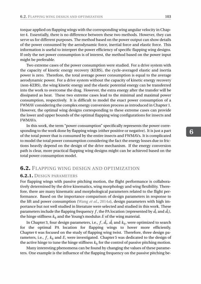
6.2. FLAPPING WING DESIGN AND OPTIMIZATION
6
103
torque applied on flapping wings with the corresponding wing angular velocity in Chap-ter 4. Essentially, there is no difference between these two methods. However, they canserve us for different purposes. The method based on the power output can show detailsof the power consumed by the aerodynamic force, inertial force and elastic force. Thisinformation is useful to interpret the power efficiency of specific flapping wing designs.If only the net power consumption is of interest, the method based on the power inputmight be preferable.
Two extreme cases of the power consumption were studied. For a drive system withthe capacity of kinetic energy recovery (KERS), the cycle-averaged elastic and inertiapower is zero. Therefore, the total average power consumption is equal to the averageaerodynamic power. For a drive system without the capacity of kinetic energy recovery(non-KERS), the wing kinetic energy and the elastic potential energy can be transferredinto the work to overcome the drag. However, the extra energy after the transfer will bedissipated as heat. These two extreme cases lead to the minimal and maximal powerconsumption, respectively. It is difficult to model the exact power consumption of aFWMAV considering the complex energy conversion process as introduced in Chapter 1.However, the optimal wing designs corresponding to these extreme cases can providethe lower and upper bounds of the optimal flapping wing configurations for insects andFWMAVs.
In this work, the term “power consumption” specifically represents the power corre-sponding to the work done by flapping wings (either positive or negative). It is just a partof the total power that is consumed by the entire insects and FWMAVs. It is complicatedto model the total power consumption considering the fact the energy losses due to fric-tions heavily depend on the design of the drive mechanism. If the energy conversionpath is clear, more practical flapping wing designs might can be achieved based on thetotal power consumption model.
6.2. FLAPPING WING DESIGN AND OPTIMIZATION
6.2.1. DESIGN PARAMETERS
For flapping wings with passive pitching motion, the flight performance is collabora-tively determined by the drive kinematics, wing morphology and wing flexibility. There-fore, there are many kinematic and morphological parameters related to the flight per-formance. Based on the importance comparison of design parameters in response tothe lift and power consumption (Wang et al., 2014a), design parameters with high im-portance but not well studied in literature were selected and studied in this work. Theseparameters include the flapping frequency f , the PA location (represented by dr and dt),the hinge stiffness kη and the Young’s modulus E of the wing material.
In Chapter 3, four design parameters, i.e., f , dr, dt and kη, were optimized to searchfor the optimal PA location for flapping wings to hover more efficiently.Chapter 4 was focused on the study of flapping wing twist. Therefore, three design pa-rameters, i.e., f , kη and E , were investigated. Chapter 5 was dedicated to the design ofthe active hinge to tune the hinge stiffness kη for the control of passive pitching motion.
Many interesting phenomena can be found by changing the values of these parame-ters. One example is the influence of the flapping frequency on the passive pitching be-
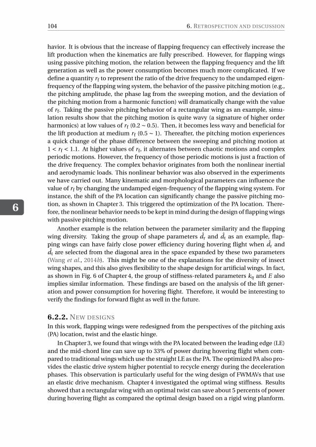
6
104 6. RETROSPECTION AND DISCUSSION
havior. It is obvious that the increase of flapping frequency can effectively increase thelift production when the kinematics are fully prescribed. However, for flapping wingsusing passive pitching motion, the relation between the flapping frequency and the liftgeneration as well as the power consumption becomes much more complicated. If wedefine a quantity rf to represent the ratio of the drive frequency to the undamped eigen-frequency of the flapping wing system, the behavior of the passive pitching motion (e.g.,the pitching amplitude, the phase lag from the sweeping motion, and the deviation ofthe pitching motion from a harmonic function) will dramatically change with the valueof rf. Taking the passive pitching behavior of a rectangular wing as an example, simu-lation results show that the pitching motion is quite wavy (a signature of higher orderharmonics) at low values of rf (0.2 ∼ 0.5). Then, it becomes less wavy and beneficial forthe lift production at medium rf (0.5 ∼ 1). Thereafter, the pitching motion experiencesa quick change of the phase difference between the sweeping and pitching motion at1 < rf < 1.1. At higher values of rf, it alternates between chaotic motions and complexperiodic motions. However, the frequency of those periodic motions is just a fraction ofthe drive frequency. The complex behavior originates from both the nonlinear inertialand aerodynamic loads. This nonlinear behavior was also observed in the experimentswe have carried out. Many kinematic and morphological parameters can influence thevalue of rf by changing the undamped eigen-frequency of the flapping wing system. Forinstance, the shift of the PA location can significantly change the passive pitching mo-tion, as shown in Chapter 3. This triggered the optimization of the PA location. There-fore, the nonlinear behavior needs to be kept in mind during the design of flapping wingswith passive pitching motion.
Another example is the relation between the parameter similarity and the flappingwing diversity. Taking the group of shape parameters dr and dt as an example, flap-ping wings can have fairly close power efficiency during hovering flight when dr anddt are selected from the diagonal area in the space expanded by these two parameters(Wang et al., 2014b). This might be one of the explanations for the diversity of insectwing shapes, and this also gives flexibility to the shape design for artificial wings. In fact,as shown in Fig. 6 of Chapter 4, the group of stiffness-related parameters kη and E alsoimplies similar information. These findings are based on the analysis of the lift gener-ation and power consumption for hovering flight. Therefore, it would be interesting toverify the findings for forward flight as well in the future.
6.2.2. NEW DESIGNS
In this work, flapping wings were redesigned from the perspectives of the pitching axis(PA) location, twist and the elastic hinge.
In Chapter 3, we found that wings with the PA located between the leading edge (LE)and the mid-chord line can save up to 33% of power during hovering flight when com-pared to traditional wings which use the straight LE as the PA. The optimized PA also pro-vides the elastic drive system higher potential to recycle energy during the decelerationphases. This observation is particularly useful for the wing design of FWMAVs that usean elastic drive mechanism. Chapter 4 investigated the optimal wing stiffness. Resultsshowed that a rectangular wing with an optimal twist can save about 5 percents of powerduring hovering flight as compared the optimal design based on a rigid wing planform.
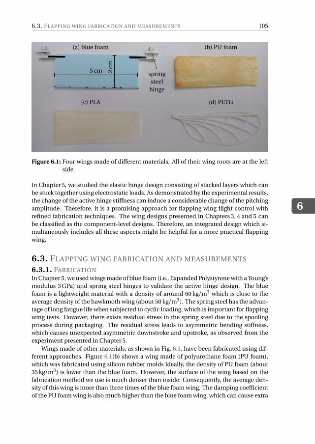
6.3. FLAPPING WING FABRICATION AND MEASUREMENTS
6
105
(a) blue foam (b) PU foam
(c) PLA (d) PETG
springsteel
hinge
5 cm 2cm
Figure 6.1: Four wings made of different materials. All of their wing roots are at the leftside.
In Chapter 5, we studied the elastic hinge design consisting of stacked layers which canbe stuck together using electrostatic loads. As demonstrated by the experimental results,the change of the active hinge stiffness can induce a considerable change of the pitchingamplitude. Therefore, it is a promising approach for flapping wing flight control withrefined fabrication techniques. The wing designs presented in Chapters 3, 4 and 5 canbe classified as the component-level designs. Therefore, an integrated design which si-multaneously includes all these aspects might be helpful for a more practical flappingwing.
6.3. FLAPPING WING FABRICATION AND MEASUREMENTS
6.3.1. FABRICATIONIn Chapter 5, we used wings made of blue foam (i.e., Expanded Polystyrene with a Young’smodulus 3 GPa) and spring steel hinges to validate the active hinge design. The bluefoam is a lightweight material with a density of around 60 kg/m3 which is close to theaverage density of the hawkmoth wing (about 50 kg/m3). The spring steel has the advan-tage of long fatigue life when subjected to cyclic loading, which is important for flappingwing tests. However, there exists residual stress in the spring steel due to the spoolingprocess during packaging. The residual stress leads to asymmetric bending stiffness,which causes unexpected asymmetric downstroke and upstroke, as observed from theexperiment presented in Chapter 5.
Wings made of other materials, as shown in Fig. 6.1, have been fabricated using dif-ferent approaches. Figure 6.1(b) shows a wing made of polyurethane foam (PU foam),which was fabricated using silicon rubber molds Ideally, the density of PU foam (about35 kg/m3) is lower than the blue foam. However, the surface of the wing based on thefabrication method we use is much denser than inside. Consequently, the average den-sity of this wing is more than three times of the blue foam wing. The damping coefficientof the PU foam wing is also much higher than the blue foam wing, which can cause extra
6
106 6. RETROSPECTION AND DISCUSSION
energy loss. The wing shown in Fig. 6.1(c) was printed in polylactic acid (PLA), whichis fairly rigid and heavy (about 1.6 g). The rigidity is helpful for experiments which ex-pect to get rid of the influence from wing flexibility, for instance, to validate the influenceof the PA location on the passive pitching behavior, as presented in Chapter 3. The 3Dprinting techniques give freedom to the wing design in terms of shape and mass distri-bution. To introduce flexibility to the printed wing, instead of using PLA, polyethyleneterephthalate glycol-modified (PETG) was used to print the wing venation as shown inFig. 6.1(d). The venation is lightweight (about 0.12 g) and flexible as a result of the favor-able properties of PETG. If combined with proper methods to integrate membrane withthe printed venation, it is a very promising approach to fabricate artificial wings withcomplex morphology.
The artificial wings we have fabricated are all full-scale (close to the adult hawkmothwing). This is because of the difficulty in using dynamically scaled wing to mimic theFSI behavior of flexible flapping wings during hovering flight. Dimensional analysis(Kang et al., 2011) shows that four dimensionless parameters have to be kept identicalbetween the real wing and the dynamically-scaled wing. These dimensionless parame-ters include the Reynolds number, reduced frequency, effective stiffness and the densityratio. Reynolds number represents the ratio between inertial forces and viscous forcesof the fluid and governs the laminar or turbulent state of the fluid. Induced frequencycompares the reference length of the wing with the spatial wavelength of the flow dis-turbance. Effective stiffness describes the ratio between flexural stiffness of the wingand moment of the fluid dynamic forces. Density ratio represents the ratio between theinertial force of wing and the fluid dynamic force. The same Reynolds number and re-duced frequency are easy to realize. However, the effective stiffness and density ratioare difficult to keep simultaneously with the Reynolds number and induced frequency.Consequently, the flexible wings in real scale are preferred for studying the interactionbetween flexible wing structures and surrounding fluid.
6.3.2. MEASUREMENTS
To validate new wing designs, we need to measure the corresponding wing kinematics,aerodynamic force and torque as well as the power consumption.
In Chapter 5, we measured the passive pitching motions with respect to differentvoltages applied on the active hinge. In this experiment, a single high-speed camera wasused, and its position and orientation were fixed such that the optical axis of the camerais perpendicular to the stroke plane of the tested wings (see Fig. 5.12). The distance oftwo chordwise markers, which changes over time on images due to the pitching motion,was used to calculate the pitching angles. However, it was hard to see the markers onimages when the chord line becomes parallel to the optical axis. This caused data lossat small pitching angles. To overcome this shortcoming, we used two cameras shoot-ing from different directions in another experiment, which aimed to check the influenceof PA location on the behavior of the passive pitching motion. The camera calibrationsand error estimation (Zhang, 2000, Hedrick, 2008) were done before measuring the wingkinematics. Due to the asymmetry introduced by the elastic hinge, there existed a dra-matic difference between the pitching motion during upstroke and downstroke. Since itwas hard to model the hinge asymmetry, we were not able to compare the experimental
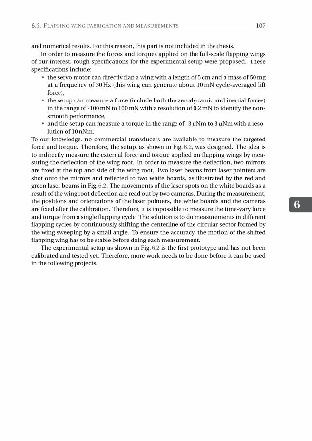
6.3. FLAPPING WING FABRICATION AND MEASUREMENTS
6
107
and numerical results. For this reason, this part is not included in the thesis.In order to measure the forces and torques applied on the full-scale flapping wings
of our interest, rough specifications for the experimental setup were proposed. Thesespecifications include:
• the servo motor can directly flap a wing with a length of 5 cm and a mass of 50 mgat a frequency of 30 Hz (this wing can generate about 10 mN cycle-averaged liftforce),
• the setup can measure a force (include both the aerodynamic and inertial forces)in the range of -100 mN to 100 mN with a resolution of 0.2 mN to identify the non-smooth performance,
• and the setup can measure a torque in the range of -3µNm to 3µNm with a reso-lution of 10 nNm.
To our knowledge, no commercial transducers are available to measure the targetedforce and torque. Therefore, the setup, as shown in Fig. 6.2, was designed. The idea isto indirectly measure the external force and torque applied on flapping wings by mea-suring the deflection of the wing root. In order to measure the deflection, two mirrorsare fixed at the top and side of the wing root. Two laser beams from laser pointers areshot onto the mirrors and reflected to two white boards, as illustrated by the red andgreen laser beams in Fig. 6.2. The movements of the laser spots on the white boards as aresult of the wing root deflection are read out by two cameras. During the measurement,the positions and orientations of the laser pointers, the white boards and the camerasare fixed after the calibration. Therefore, it is impossible to measure the time-vary forceand torque from a single flapping cycle. The solution is to do measurements in differentflapping cycles by continuously shifting the centerline of the circular sector formed bythe wing sweeping by a small angle. To ensure the accuracy, the motion of the shiftedflapping wing has to be stable before doing each measurement.
The experimental setup as shown in Fig. 6.2 is the first prototype and has not beencalibrated and tested yet. Therefore, more work needs to be done before it can be usedin the following projects.
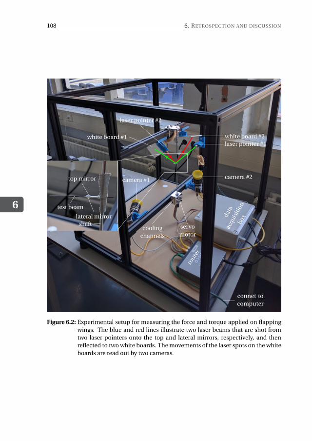
6
108 6. RETROSPECTION AND DISCUSSION
data
acqu
isiti
onbo
x
route
r
connet tocomputer
servomotor
coolingchannels
shaft
test beam
top mirror
lateral mirror
camera #1 camera #2
laser pointer #1
laser pointer #2
white board #1 white board #2
Figure 6.2: Experimental setup for measuring the force and torque applied on flappingwings. The blue and red lines illustrate two laser beams that are shot fromtwo laser pointers onto the top and lateral mirrors, respectively, and thenreflected to two white boards. The movements of the laser spots on the whiteboards are read out by two cameras.

7GENERAL CONCLUSIONS AND
RECOMMENDATIONS
The previous chapter retrospected and discussed the most important aspects related to themodeling, design and optimization of flapping wings for efficient hovering flight. In thischapter, the overall conclusions will be drawn and recommendations for further study willbe provided.
109
7
110 7. GENERAL CONCLUSIONS AND RECOMMENDATIONS
7.1. CONCLUSIONSIn this thesis, we have worked towards more power-efficient flapping wing designs forhovering flight as compared to most existing wing designs. Progress has been made onthe wing modeling, design and optimization.
We have proposed a quasi-steady aerodynamic model for flapping wings, particu-larly for wings with passive pitching motion. The quasi-steady model can accurately pre-dict both the aerodynamic loads and the corresponding center of pressure. The modeldoes not rely on any empirical parameters and can be used to evaluate the aerodynamicperformance of wings with different shapes and kinematics. To further enable the para-metric study and optimization of twistable flapping wings, a computationally efficientfluid-structure interaction model was also proposed by using the quasi-steady aerody-namic model and an analytical twist model. It has been shown that a quadratic polyno-mial can accurately model the twist of a rectangular wing with large twist amplitudes.
It has been shown that, for wings with passive pitching motion, the pitching axislocation plays a very important role for power efficiency of hovering flight. Compar-isons show that an optimal pitching axis can save up to 33% of power when comparedto traditional wings with optimal kinematics but a straight leading edge as the pitchingaxis. With the optimized pitching axis, flapping wings show high pitching amplitudesand start the pitching reversal in advance of the sweeping reversal. These phenomenalead to high lift-to-drag ratios and explain the low power consumption. In addition, theoptimized pitching axis provides the drive system higher potential to recycle kinetic en-ergy during the deceleration phases as compared to traditional wings. This is becausethe aerodynamic power before pitching reversals is negligible for wings with optimal PA,while the traditional wings still experience a significant amount of aerodynamic powerconsumption before reversals. This observation underlines the particular importance ofthe wing pitching axis location for power-efficient FWMAVs when using kinetic energyrecovery drive systems.
We have also shown that the optimized twistable wings can not dramatically out-perform the optimized rigid wings in terms of the power efficiency, unless the pitchingamplitude at the wing root is limited. With the decrease of the pitching amplitude atthe root, the optimized rigid wings need more power for hovering. However, the opti-mized twistable wings can always maintain high power efficiency by introducing a cer-tain amount of twist to increase the overall pitching amplitude. Moreover, the high com-putational efficiency of the proposed FSI model allows to study the flexibility of insectwings and help the wing design for FWMAVs.
A promising method to actively control the passive pitching motion of a flappingwing has also been presented by using electrostatic control of the stiffness of the wingelastic hinge. The hinge is realized by stacking three conducting spring steel layers whichare separated by dielectric Mylar films. Our theoretical model shows that the stackedlayers can switch from slipping with respect to each other to sticking together whenthe electrostatic load between layers, which can be controlled by the applied voltage,is above a threshold value. The switch can result in a dramatic increase of the hinge stiff-ness (about 9×) such that a short duration of the sticking still can lead to a considerablechange of the passive pitching motion. Experimental results successfully confirmed thedecrease of the pitching amplitude with the increase of the applied voltages. Moreover,
7.2. RECOMMENDATIONS
7
111
flight control based on electrostatically controlled hinges can be very power-efficientsince there is, ideally, no power consumption associated with the control operations.
7.2. RECOMMENDATIONSAs retrospected, we have provided some approaches to achieve power-efficient flappingwing designs for hovering flight. However, there are still many open questions and chal-lenges concerning the wing modeling, design, optimization, fabrication and testing.
The proposed quasi-steady aerodynamic model was validated for rigid wings. How-ever, how to integrate the influence of wing camber and bending into the model needs tobe investigated. In addition, the clap-and-fling phenomenon exists for the four-wingedAtalanta FWMAV. Therefore, it is also useful to include the clap-and-fling mechanisminto the model to reflect the interactions between adjacent wings. The challenge is howto integrate these extra terms into the model using as less empirical parameters as pos-sible.
The proposed FSI model generally overestimates the wing stiffness as a result of theassumptions used by the analytical twist model. The overestimation can be reducedby using more accurate formulations to describe the spanwise wing displacement andallowing the chord length to change with the twist angle. In addition, the FSI modelhas two limitations. First, the model is limited to wings with uniform thickness. Thislimitation can be eliminated by updating the plate model by including the influence ofthe thickness variation. Second, for extremely large twist, the accuracy of the proposedFSI model can not be guaranteed since the plate theory for a moderate deformation isused. To overcome this limitation, one cheap solution is to divide the whole wing intofinite parts and virtually connect adjacent parts with torsional springs. The proposedFSI model can be applied to each part separately. As a consequence, the wing displace-ment at the connection edges will be not differentiable, which might introduce someartificial stiffness. However, this extended model can be very useful to study the twistof insect wings that consist of a fore-wing and a hind-wing, like hawkmoth wings. Withthe extended quasi-steady aerodynamic model, we can extend the proposed FSI modelas well. To do so, the elastic deformation needs to be updated to take the camber andbending into consideration.
The dynamic behavior of the passive pitching motion can vary dramatically for dif-ferent values of the undamped frequency ratio of the flapping wing system. The changesof the pitching motion can be reflected by the pitching amplitude, output frequency, sta-tus of convergence, phase lag between the pitching and sweeping motion. The frequencyratio is influenced by many factors, including the drive frequency, the wing stiffness, thewing pitching axis location and the mass distribution. It is useful to further study (1)how to achieve a robust wing design by keeping the wing working in a range where thepitching motion is the least sensitive to the influential factors, and (2) how to make useof the sensitivity of the passive pitching motion with respect to the influential factors forcontrol purposes.
In this work, we assume that both the sweeping motion and the wing stiffness whenbended to both sides are symmetric. Therefore, the passive pitching motion is also sym-metric. However, it is quite common to have asymmetric sweeping motion, pitchingmotion and wing stiffness for insect wings. More complex descriptions of the sweeping
112 7. GENERAL CONCLUSIONS AND RECOMMENDATIONS
motion and the wing stiffness should be introduced to better study insect wings. Forinstance, two harmonic functions with a same frequency but different amplitudes canbe used to describe the sweeping motion in two half-strokes, respectively. A quadraticpolynomial can be used to achieve asymmetric wing root stiffness, while the cubic poly-nomial term can introduce extra nonlinear effect to the wing root stiffness.
An interesting phenomenon was observed during the wing shape and stiffness opti-mization when two of the design variables are of similar characteristics (e.g., dr and dt, kηand E). If we plot the contour lines corresponding to the lift constraint function and thepower consumption on the plane expanded by these two variables, it can be observedthat the zero lift contour line is approximately parallel to the nearby power contour lines.Therefore, different combinations of these two variables can result in similar power effi-ciency. It would be interesting to investigate the relation between this phenomenon withthe diversity of the wing morphology in nature.
The models proposed in this thesis can provide an optimal wing shape and stiffnesscorresponding to minimal power consumption. However, there is still a gap betweenthese optimal wing designs and the realization of these wings. To bridge the gap, anintegrated design which considers both the wing shape and stiffness is required, andmore advanced structural design or optimization techniques need to be applied. Forinstance, if a carbon-fiber-reinforced-membrane wing is expected for the final wing de-sign, an integrated optimization need to be conducted by directly using an appropriatewing stiffness model for this type of wing. If a freeform wing structure is wanted, topol-ogy optimization technique can be used to automate the wing structural design.
For the active hinge design, the fabrication process needs to be optimized by us-ing well-designed tools to reduce manufacturing inaccuracies. It is also interesting toconduct long-lasting experiments to study the influence of wear between the Mylar andconducting sheets. The ultimate aim of the wing design is to realize workable flappingwings. Therefore, the testing of the designed wings is very important. The testing shouldinclude the aerodynamic force generation, the power efficiency and the strength of thefabricated wing.
ADERIVATION OF RELATION
BETWEEN 2D AND 3D LIFT
COEFFICIENTS
Based on the discretized wing using the blade element method (BEM), the resultant lifton a rigid flapping wing can be calculated by
Ltrans =∫ R
0
1
2ρfv2C trans
l cd xc , (A.1)
where the 2D lift coefficient C transl is a constant for a given angle of attack. Considering
the fact that along the span v =ωzi xc , above equation can be rewritten as
Ltrans = 1
2ρfω2
ziR2r 2
2 C transl S, (A.2)
where S is the wing area (= ∫ R0 cd xc ), and r2 is the span-normalized distance from the
root chord to the gyradius which is given by
r2 =√
1
SR2
∫ R
0x2
c cd xc . (A.3)
When the translation velocity at the gyradius is taken as the reference velocity, the liftforce based on 3D lift coefficient C trans
L can be written as
Ltrans = 1
2ρf (r2Rωzi
)2 C transL S. (A.4)
By comparing Eqs. A.2 and A.4, it can be seen found that C transL can be used directly
as the 2D lift coefficient C transl for the BEM as long as the reference velocity is at gyration.
113

BDERIVATION OF AERODYNAMIC
LOAD ON A UNIFORMLY ROTATING
PLATE IMMERSED IN AN INCOMING
FLOW
To derive the loads experienced by a plate uniformly rotating around its pitching axis atzero angle of attack (AOA) when immersed in an incoming flow with a velocity of vzc , theacceleration potential method is used (Fung, 1993). Assuming that the rotational angle isinfinitesimal and the velocity of the incoming flow is much higher than the rotational ve-locity, the horizontal offset of the plate due to the rotation is negligible. Setting the timewith respect to zero AOA to be t = 0, the plate position can be described as a function oftime
yw =ωxc t(xw + cd − c
2
), − c
2≤ xw ≤ c
2, (B.1)
where xw and yw are axes of the introduced frame as shown in Fig. B.1.The fluid surrounding the plate needs to satisfy three boundary conditions (BCs):
(1) the flow on its surface must be tangent to the plate both in the velocity and accel-eration field; (2) the Kutta condition has to be satisfied at the trailing edge (TE); (3) thefluid acceleration at infinity should be zero. For inviscid and incompressible flow, themomentum equation can be written as
af =∇ (Φ) , (B.2)
where af represents the fluid acceleration, and Φ is the acceleration potential which isequal to −p/ρf. This implies that the static pressure p is proportional to the accelera-tion potential Φ. Meanwhile, there exists a conjugate function Ψ orthogonal to Φ andsatisfying
∂Φ
∂xw= ∂Ψ
∂yw= vxw ,
∂Φ
∂yw=− ∂Ψ
∂xw= vyw . (B.3)
115
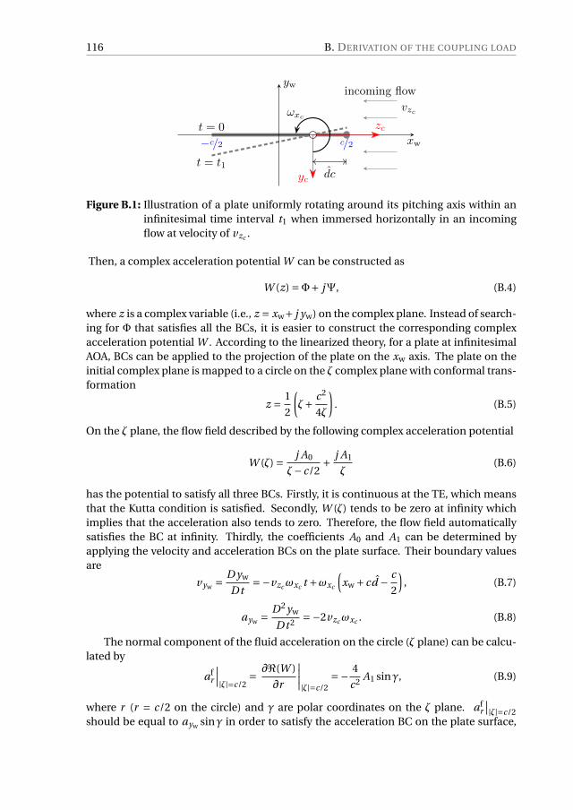
116 B. DERIVATION OF THE COUPLING LOAD
−c/2 c/2 xw
yw
yc
zct = 0
t = t1
vzc
incoming flow
ωxc
dc
Figure B.1: Illustration of a plate uniformly rotating around its pitching axis within aninfinitesimal time interval t1 when immersed horizontally in an incomingflow at velocity of vzc .
Then, a complex acceleration potential W can be constructed as
W (z) =Φ+ jΨ, (B.4)
where z is a complex variable (i.e., z = xw+ j yw) on the complex plane. Instead of search-ing for Φ that satisfies all the BCs, it is easier to construct the corresponding complexacceleration potential W . According to the linearized theory, for a plate at infinitesimalAOA, BCs can be applied to the projection of the plate on the xw axis. The plate on theinitial complex plane is mapped to a circle on the ζ complex plane with conformal trans-formation
z = 1
2
(ζ+ c2
4ζ
). (B.5)
On the ζ plane, the flow field described by the following complex acceleration potential
W (ζ) = j A0
ζ− c/2+ j A1
ζ(B.6)
has the potential to satisfy all three BCs. Firstly, it is continuous at the TE, which meansthat the Kutta condition is satisfied. Secondly, W (ζ) tends to be zero at infinity whichimplies that the acceleration also tends to zero. Therefore, the flow field automaticallysatisfies the BC at infinity. Thirdly, the coefficients A0 and A1 can be determined byapplying the velocity and acceleration BCs on the plate surface. Their boundary valuesare
vyw = D yw
Dt=−vzcωxc t +ωxc
(xw + cd − c
2
), (B.7)
ayw = D2 yw
Dt 2 =−2vzcωxc . (B.8)
The normal component of the fluid acceleration on the circle (ζ plane) can be calcu-lated by
afr
∣∣∣|ζ|=c/2= ∂ℜ(W )
∂r
∣∣∣∣|ζ|=c/2=− 4
c2 A1 sinγ, (B.9)
where r (r = c/2 on the circle) and γ are polar coordinates on the ζ plane. afr
∣∣|ζ|=c/2should be equal to ayw sinγ in order to satisfy the acceleration BC on the plate surface,
117
whereby the coefficient A1 is obtained as
A1 =1
2vzcωxc c2. (B.10)
The velocity BC can be used to calculate the coefficient A0. The fluid velocity v fyw
on theplate in the ζ plane can be calculated by solving the partial differentiation equation
∂v fyw
∂t− vzc
∂v fyw
∂xw= af
yw=− ∂Ψ
∂xw. (B.11)
The fluid velocity on the plate can be obtained as
v fyw
= Ψ
vzc
+h(vzc t +xw), (B.12)
where h(·) can be an arbitrary function of the expression vzc t + xw, and Ψ is equal to2vzcωxc xw − A0/c which is obtained from Eq. B.6 by substituting ζ with z which is deter-mined by xw and yw. If we let h(vzc t + xw) be −ω(vzc t + xw), and apply the velocity BCthat the fluid velocity v f
ywis equal to the boundary value of the velocity given in Eq. B.7
over the plate except for the singular point at the LE, we get
A0 = vzcωxc c2(
1
2− d
). (B.13)
Substituting Eqs. B.10 and B.13 into B.6, the acceleration potentialΦ can be obtainedas
Φ= vzcωxc c sin(γ)−2vzcωxc sin(γ)c(d − 1
2 )
(1−cos(γ))2 + sin2(γ)(B.14)
with which the pressure distribution can be calculated. Eventually, the lift L and torqueτ about the pitching axis due to the coupling effect on a plate with unity span can beobtained by integrating the pressure over the entire circle on the ζ plane, resulting in,
L =πρfvzcωxc c2(
3
4− d
)+ 1
4πρvzcωxc c2, (B.15)
τ=πρfvzcωxc c3(
3
4− d
)(1
4− d
)+ 1
4πρvzcωxc c3
(3
4− d
), (B.16)
from which it can be seen that the lift consists of two components which act at the1/4 chord and 3/4 chord, respectively. The first component can be regarded as a re-sult of a wing rotation-induced vorticity concentrated at the 1/4 chord while satisfyingthe boundary condition for the downwash at the 3/4 chord location, and the secondcomponent is a result of Coriolis effect experienced by the fluid with equivalent massof 1
4πρfc2 while flowing on a rotating wing. It should be noted that τ is, by convention,
considered to be positive when it acts to pitch the plate in the nose-up direction.

CDERIVATION OF GOVERNING
EQUATION FOR PASSIVE PITCHING
MOTION OF A RIGID WING
In this Appendix, the equation of motion that governs the passive pitching motion offlapping wings is derived.
Generally, the passive pitching motion is achieved by connecting the wing to thedrive mechanism with an elastic hinge while the drive mechanism applies a sweepingtorque. Then, the wing is forced to pitch about the pitching axis by the wing inertiaand aerodynamic loads. Since the out-of-plane motion is not completely constrained,a slight heaving motion might be observed, as shown in the second validation case. In-deed, the heaving motion has a small contribution to the drive torque and the passivepitching motion. The contribution of gravity to the passive pitching motion is ignoreddue to the small wing mass and the fact that the centre of mass is not far away from thepitching axis.
Since the moment of inertia I of the wing is constant in the co-rotating frame, Euler’ssecond law of motion for a rigid body is applied about the pitching axis of the wing (i.e.,xc axis), namely,
τappliedxc
+τinerxc
= 0, (C.1)
where τappliedxc
consists of the elastic torque τelasxc
(=−kηη) from the hinge and the aerody-namic torque τaero
xcwhich includes four parts as presented in Section 2.2.2. The inertial
torque in the co-rotating frame can be calculated by
τiner =−Iαc −ωc × (Iωc ) , (C.2)
whereωc andαc are the angular velocity and acceleration in the co-rotating frame, andthe two components are the torque due to Euler and Coriolis forces, respectively. The
119
120 C. DERIVATION OF GOVERNING EQUATION FOR PASSIVE PITCHING MOTION
component of τiner on xc axis can be divided into the term −Ixc xc η and the inertial drivetorque τdrive
xcwhich can be expressed as
τdrivexc
= Ixc xc
[1
2φ2 cos2θ sin(2η)− 1
2θ2 sin(2η)+2φθcosθcos2η+ φsinθ
]+
Ixc zc
[θ sinη+ 1
2φ2 sin(2θ)sinη− φcosθcosη+2φθ sinθcosη
]. (C.3)
Eventually, the equation of motion of the wing pitching can be expressed as
Ixc xc η+kηη= τaeroxc
+τdrivexc
. (C.4)
REFERENCES
ALLEN, H. G. 1969 Analysis and design of structural sandwich panels. Pergamon.
ANDERSEN, A., PESAVENTO, U. & WANG, Z. J. 2005 Unsteady aerodynamics of flutteringand tumbling plates. Journal of Fluid Mechanics 541, 65–90.
ANDERSON, J. 2010 Fundamentals of Aerodynamics. McGraw-Hill Education.
ANSARI, S. A. 2004 A nonlinear, unsteady, aerodynamic model for insect-like flappingwings in the hover with micro air vehicle applications. Phd thesis, Cranfield University.
ANSARI, S. A., BIKOWSKI, R. & KNOWLES, K. 2006 Aerodynamic modelling of insect-likeflapping flight for micro air vehicles. Progress in Aerospace Sciences 42 (2), 129–172.
ANSARI, S. A., KNOWLES, K. & ZBIKOWSKI, R. 2008 Insectlike Flapping Wings in theHover Part II: Effect of Wing Geometry. Journal of Aircraft 45 (6), 1976–1990.
APPEL, E. & GORB, S. N. 2011 Resilin-bearing wing vein joints in the dragonfly Epio-phlebia superstes. Bioinspiration & biomimetics 6, 046006.
BERGAMINI, A., CHRISTEN, R., MAAG, B. & MOTAVALLI, M. 2006 A sandwich beam withelectrostatically tunable bending stiffness. Smart Materials and Structures 15 (3), 678–686.
BERGOU, A. J., XU, S. & WANG, Z. J. 2007 Passive wing pitch reversal in insect flight.Journal of Fluid Mechanics 591, 321–337.
BERMAN, G. J. & WANG, Z. J. 2007 Energy-minimizing kinematics in hovering insectflight. Journal of Fluid Mechanics 582, 153–168.
BETTS, C. R. & WOOTTON, R. J. 1988 Wing shape and flight behaviour in butterflies (Lep-idoptera: Papilionoidea and Hesperioidea): a preliminary analysis. Journal of Experi-mental Biology 288 (1), 271–288.
BIRCH, J. M. & DICKINSON, M. H. 2001 Spanwise flow and the attachment of theleading-edge vortex on insect wings. Nature 412 (6848), 729–733.
BOLSMAN, C. T. 2010 Flapping wing actuation using resonant compliant mechanisms,an insect inspired design. Doctoral thesis, Technische Universiteit Delft.
BOLSMAN, C. T., GOOSEN, J. F. L. & VAN KEULEN, F. 2009 Design overview of a resonantwing actuation mechanism for application in flapping wing MAVs. International Jour-nal of Micro Air Vehicles 1 (4), 263–272.
BRENNEN, C. E. 1982 A review of added mass and fluid inertial forces. Tech. Rep.. NavalCivil Engineering Laboratory, Port Hueneme, California.
CHABRIER, J. 1822 Essai sur le vol des insectes, et observations. Kessinger Publishing.
CHANUTE, O. 1894 Progress in Flying Machines. Courier Corporation.
CHAUDHURI, A., HAFTKA, R., IFJU, P. G., VILLANUEVA, D., CHANG, K. & RUE, J. 2013 Ex-perimental Optimization and Uncertainty Quantification of Flapping Wing of a MicroAir Vehicle. In 10th World Congress on Structural and Multidisciplinary Optimization,pp. 1–10. Orlando, Florida, USA.
121
122 REFERENCES
CHEN, Y., SKOTE, M., ZHAO, Y. & HUANG, W. 2013 Dragonfly (Sympetrum flaveolum)flight: Kinematic measurement and modelling. Journal of Fluids and Structures 40,115–126.
CLARK, W. W. 2000 Vibration Control with State-Switched Piezoelectric Materials. Jour-nal of Intelligent Material Systems and Structures 11 (4), 263–271.
COMBES, S. A. & DANIEL, T. L. 2003 Flexural stiffness in insect wings. II. Spatial distribu-tion and dynamic wing bending. The Journal of experimental biology 206, 2989–2997.
DE CROON, G. C. H. E., DE CLERCQ, K. M. E., RUIJSINK, R., REMES, B. & DE WAGTER,C. 2009 Design, aerodynamics, and vision-based control of the DelFly. InternationalJournal of Micro Air Vehicles 1 (2), 71–98.
DAI, H., LUO, H. & DOYLE, J. F. 2012 Dynamic pitching of an elastic rectangular wing inhovering motion. Journal of Fluid Mechanics 693, 473–499.
DICKINSON, M. H. & GÖTZ, K. G. 1993 Unsteady aerodynamic performance of modelwings at low Reynolds numbers. Journal of Experimental Biology 64, 45–64.
DICKINSON, M. H., LEHMANN, F. O. & SANE, S. P. 1999 Wing rotation and the aerody-namic basis of insect flight. Science 284 (5422), 1954–1960.
DICKSON, W. B., STRAW, A. D., POELMA, C. & DICKINSON, M. H. 2006 An integrativemodel of insect flight control. In Proceedings of the AIAA Aerospace Sciences Meetingand Exhibit, pp. 1–19. Reno, NV.
DONOUGHE, S., CRALL, J. D., MERZ, R. A. & COMBES, S. A. 2011 Resilin in dragonflyand damselfly wings and its implications for wing flexibility. Journal of morphology272 (12), 1409–21.
DU, G. & SUN, M. 2008 Effects of unsteady deformation of flapping wing on its aerody-namic forces. Applied Mathematics and Mechanics 29 (6), 731–743.
DU, G. & SUN, M. 2010 Effects of wing deformation on aerodynamic forces in hoveringhoverflies. The Journal of experimental biology 213, 2273–2283.
DUDLEY, R. 2002 The biomechanics of insect flight: form, function, evolution. PrincetonUniversity Press.
DUDLEY, R. & ELLINGTON, C. P. 1990 Mechanics of Forward Flight in Bumblebees: I.Kinematics and Morphology. Journal of Experimental Biology 148 (1), 19–52.
ELDREDGE, J. D., WANG, C. & OL, M. V. 2009 A computational study of a canonical pitch-up, pitch-down wing maneuver. In 39th AIAA Fluid Dynamics Conference, pp. 1–14.San Antonio, Texas.
ELLINGTON, C. P. 1984a The Aerodynamics of Hovering Insect Flight. II. Morphologi-cal Parameters. Philosophical Transactions of the Royal Society B: Biological Sciences305 (1122), 17–40.
ELLINGTON, C. P. 1984b The Aerodynamics of Hovering Insect Flight. III. Kinematics.Philosophical Transactions of the Royal Society B: Biological Sciences 305 (1122), 145–181.
ELLINGTON, C. P. 1984c The aerodynamics of hovering insect flight. IV. aeorodynamicmechanisms. Philosophical Transactions of the Royal Society B: Biological Sciences305 (1122), 79–113.
ELLINGTON, C. P. 1984d The aerodynamics of hovering insect flight. V. a vortex theory.Philosophical Transactions of the Royal Society B: Biological Sciences 305 (1122), 115–144.
REFERENCES 123
ELLINGTON, C. P. 1999 The novel aerodynamics of insect flight: applications to micro-airvehicles. The Journal of experimental biology 202, 3439–3448.
ELLINGTON, C. P., VAN DEN BERG, C., WILLMOTT, A. P. & THOMAS, A. L. R. 1996 Leading-edge vortices in insect flight. Nature 384 (6610), 626–630.
ENNOS, A. R. 1989 Inertial and aerodynamic torques on the wings of diptera in flight. J.Exp. Biol. 142 (1), 87–95.
FINIO, B. M. & WOOD, R. J. 2012 Open-loop roll, pitch and yaw torques for a roboticbee. In 2012 IEEE/RSJ International Conference on Intelligent Robots and Systems, pp.113–119. Vilamoura, Algarve, Portugal: IEEE.
FLOREANO, D. & WOOD, R. J. 2015 Science, technology and the future of small au-tonomous drones. Nature 521 (7553), 460–466.
FORD, C. W. P. & BABINSKY, H. 2014 Impulsively started flat plate circulation. AIAA Jour-nal 52 (8), 1800–1802.
FREE FLIGHT SUPPLIES 2015 www.freeflightsupplies.co.uk/mylarspec.pdf.FUNG, Y. C. 1993 An introduction to the theory of aeroelasticity. Courier Dover Publica-
tions.GOLDFARB, M. & SPEICH, J. E. 1999 A Well-Behaved Revolute Flexure Joint for Compliant
Mechanism Design. Journal of Mechanical Design 121 (3), 424.GRAY, C. 2003 Leonardo da Vinci, http://www.flyingmachines.org/davi.html.HA, N. S., TRUONG, Q. T., PHAN, H. V., GOO, N. S. & PARK, H. C. 2014 Structural Char-
acteristics of Allomyrina Dichotoma Beetle’s Hind Wings for Flapping Wing Micro AirVehicle. Journal of Bionic Engineering 11 (2), 226–235.
HAN, J. S., KIM, J. K., CHANG, J. W. & HAN, J. H. 2015 An improved quasi-steady aero-dynamic model for insect wings that considers movement of the center of pressure.Bioinspiration & Biomimetics 10, 046014.
HARBIG, R. R., SHERIDAN, J. & THOMPSON, M. C. 2014 The role of advance ratio andaspect ratio in determining leading-edge vortex stability for flapping flight. Journal ofFluid Mechanics 751, 71–105.
HEDRICK, T. L. 2008 Software techniques for two- and three-dimensional kinematicmeasurements of biological and biomimetic systems. Bioinspiration & biomimetics3, 034001.
VAN DEN HEUVEL, H. 2015 Conceptual Development of a Catalytic Expansion Actuatorfor a Resonating-body Flapping-wing Micro Air Vehicle. Master’s thesis.
HOFF, W. 1919 Der flug der insekten und der vögel. Die Naturwissenschaften 7 (10), 159–162.
HOU, D., YIN, Y., ZHAO, H. & ZHONG, Z. 2015 Effects of blood in veins of dragonfly wingon the vibration characteristics. Computers in Biology and Medicine 58, 14–19.
HOWELL, L. L. 2001 Compliant mechanisms. John Wiley & Sons.ISHIHARA, D., HORIE, T. & DENDA, M. 2009 A two-dimensional computational study on
the fluid–structure interaction cause of wing pitch changes in dipteran flapping flight.Journal of Experimental Biology 212, 1–10.
JOHANSSON, L. C., ENGEL, S., KELBER, A., HEERENBRINK, M. K. & HEDENSTRÖM, A.2013 Multiple leading edge vortices of unexpected strength in freely flying hawkmoth.Scientific reports 3, 3264.
JONES, R. T. 1940 The unsteady lift of a wing of finite aspect ratio. Tech. Rep..
124 REFERENCES
JUDY, J. W. 2001 Microelectromechanical systems (MEMS): fabrication, design and ap-plications. Smart Materials and Structures 10 (6), 1115–1134.
KANG, C. K., AONO, H., CESNIK, C. E. S. & SHYY, W. 2011 Effects of Flexibility on theAerodynamic Performance of Flapping Wings. In 6th AIAA Theoretical Fluid Mechan-ics Conference, pp. 1–46. Honolulu, Hawaii.
KEENNON, M., KLINGEBIEL, K. & WON, H. 2012 Development of the Nano Humming-bird: A Tailless Flapping Wing Micro Air Vehicle. In 50th AIAA Aerospace Sciences Meet-ing including the New Horizons Forum and Aerospace Exposition, pp. 1–24. Nashville,Tennessee.
KELLY, M. 2006 Steam in the Air: The Application of Steam Power in Aviation During the19th and 20th Centuries. Casemate Publishers.
LAU, G. K., CHIN, Y. W., GOH, J. T. W. & WOOD, R. J. 2014 Dipteran-insect-inspiredthoracic mechanism with nonlinear stiffness to save inertial power of flapping-wingflight. IEEE Transactions on Robotics 30 (5), 1187–1197.
LEE, J., CHOI, H. & KIM, H. Y. 2015 A scaling law for the lift of hovering insects. Journalof Fluid Mechanics 782, 479–490.
LEHMANN, F. O. 2008 When wings touch wakes: understanding locomotor force controlby wake wing interference in insect wings. The Journal of experimental biology 211,224–233.
LEHMANN, F. O. & PICK, S. 2007 The aerodynamic benefit of wing-wing interaction de-pends on stroke trajectory in flapping insect wings. The Journal of experimental biol-ogy 210, 1362–1377.
LI, H.-S. & AU, S.-K. 2010 Design optimization using Subset Simulation algorithm.Structural Safety 32 (6), 384–392.
LILIENTHAL, O. 1895 lilienthal.
MA, K. Y., CHIRARATTANANON, P., FULLER, S. B. & WOOD, R. J. 2013 Controlled flight ofa biologically inspired, insect-scale robot. Science 340 (6132), 603–607.
MA, K. Y., FELTON, S. M. & WOOD, R. J. 2012 Design, fabrication, and modeling of thesplit actuator microrobotic bee. In 2012 IEEE/RSJ International Conference on Intelli-gent Robots and Systems, pp. 1133–1140. Vilamoura, Algarve, Portugal.
MAJIDI, C. & WOOD, R. J. 2010 Tunable elastic stiffness with microconfined magne-torheological domains at low magnetic field. Applied Physics Letters 97, 164104.
MARTÍ-CAMPOY, A., ÁVALOS, J. A., SOTO, A., RODRÍGUEZ-BALLESTER, F., MARTÍNEZ-BLAY, V. & MALUMBRES, M. P. 2016 Design of a Computerised Flight Mill Device toMeasure the Flight Potential of Different Insects. Sensors 16 (485), 1–21.
MENG, X. G. & SUN, M. 2015 Aerodynamics and vortical structures in hovering fruitflies.Physics of Fluids 27 (031901), 1–22.
MUIJRES, F. T., ELZINGA, M. J., MELIS, J. M. & DICKINSON, M. H. 2014 Flies evade loom-ing targets by executing rapid visually directed banked turns. Science 344, 172–177.
NABAWY, M. R. A. & CROWTHER, W. J. 2014 On the quasi-steady aerodynamics of nor-mal hovering flight part II: model implementation and evaluation. Journal of the RoyalSociety Interface 11 (20131197), 1–9.
NAKATA, T. & LIU, H. 2012a A fluid–structure interaction model of insect flight with flex-ible wings. Journal of Computational Physics 231 (4), 1822–1847.
REFERENCES 125
NAKATA, T. & LIU, H. 2012b Aerodynamic performance of a hovering hawkmoth withflexible wings: a computational approach. Proceedings of the Royal Society B: Biologi-cal Sciences 279, 722–731.
NEWMAN, J. N. 1977 Marine hydrodynamics. The MIT Press.
NGUYEN, Q.-V., CHAN, W. L. & DEBIASI, M. 2015 An insect-inspired flapping wing microair vehicle with double wing clap-fling effects and capability of sustained hovering.In Proc. SPIE 9429, Bioinspiration, Biomimetics, and Bioreplication (ed. A. Lakhtakia,M. Knez & R. J. Martín-Palma), pp. 1–11. San Diego, California, United States.
OSBORNE, M. F. M. 1951 Aerodynamics of flapping flight with application to insects.Journal of Experimental Biology 28, 221–245.
PERCIN, M. & VAN OUDHEUSDEN, B. W. 2015 Three-dimensional flow structures andunsteady forces on pitching and surging revolving flat plates. Experiments in Fluids56 (47), 1–19.
PETERS, H. J., GOOSEN, J. F. L. & VAN KEULEN, F. 2016 Methods to actively modify thedynamic response of cm-scale FWMAV designs. Smart Materials and Structures 25 (5),055027.
PETERS, H. J., WANG, Q., GOOSEN, J. F. L. & VAN KEULEN, F. 2015 Active control of thepassive pitching of a flapping wing with electrostatic clamping. In 7th ECCOMAS The-matic Conference on Smart Structures and Materials (SMART 2015), pp. 1–19. Azores,Portugal.
PITT FORD, C. W. & BABINSKY, H. 2013 Lift and the leading-edge vortex. Journal of FluidMechanics 720, 280–313.
RISTROPH, L. & CHILDRESS, S. 2014 Stable hovering of a jellyfish-like flying machine.Journal of the Royal Society, Interface 11 (20130992), 1–7.
SANE, S. P. 2003 The aerodynamics of insect flight. Journal of Experimental Biology206 (23), 4191–4208.
SANE, S. P. & DICKINSON, M. H. 2002 The aerodynamic effects of wing rotation and arevised quasi-steady model of flapping flight. J. Exp. Biol. 205 (8), 1087–1096.
SCHLICHTING, H. & TRUCKENBRODT, E. A. 1979 Aerodynamics of the aeroplane, 2nd edn.McGraw Hill Higher Education.
SCHWAB, A. L. & MEIJAARD, J. P. 2006 How to draw Euler angles and utilize Euler pa-rameters. In Proceedings of IDETC/CIE ASME 2006 International Design EngineeringTechnical Conferences & Computers and Information in Engineering Conference, pp.1–7. Philadelphia, Pennsylvania, USA.
SELVAN, A. 2014 Simulation of optic flow based flight control for a flapping wing microaerial vehicle. Master’s thesis.
SESHADRI, P., BENEDICT, M. & CHOPRA, I. 2013 Understanding Micro Air VehicleFlapping-Wing Aerodynamics Using Force and Flowfield Measurements. Journal ofAircraft 50 (4), 1070–1087.
SHAHZAD, A., TIAN, F.-B., YOUNG, J. & LAI, J. C. S. 2016 Effects of wing shape, aspectratio and deviation angle on aerodynamic performance of flapping wings in hover.Physics of Fluids 28 (111901), 1–36.
SHAW, W. H. & RUHEN, O. 1977 Lawrence Hargrave: explorer, inventor & aviation exper-imenter. Cassell Australia Ltd.
126 REFERENCES
SHYY, W., AONO, H., CHIMAKURTHI, S. K., TRIZILA, P., KANG, C. K., CESNIK, C. E. S.& LIU, H. 2010 Recent progress in flapping wing aerodynamics and aeroelasticity.Progress in Aerospace Sciences 46 (7), 284–327.
SREETHARAN, P. S., WHITNEY, J. P., STRAUSS, M. D. & WOOD, R. J. 2012 Monolithic fabri-cation of millimeter-scale machines. Journal of Micromechanics and Microengineering22 (055027), 1–6.
STEWART, E., PATIL, M., CANFIELD, R. & SNYDER, R. 2013 Shape Optimization of a Flap-ping Wing. In 54th AIAA/ASME/ASCE/AHS/ASC Structures, Structural Dynamics, andMaterials Conference, pp. 1–11. Boston, Massachusetts.
SUN, M. 2014 Insect flight dynamics: Stability and control. Reviews of Modern Physics86 (2), 615–646.
TABATA, O., KONISHI, S., CUSIN, P., ITO, Y., KAWAI, F., HIRAI, S. & KAWAMURA, S. 2001Micro fabricated tunable bending stiffness devices. Sensors and Actuators A: Physical89, 119–123.
TAHA, H. E., HAJJ, M. R. & BERAN, P. S. 2014 State-space representation of the unsteadyaerodynamics of flapping flight. Aerospace Science and Technology 34 (1), 1–11.
TANAKA, H. 2012 Flexible wing structures of simplified insect-sized flapping MAVs. InProceedings of 2012ICME International Conference on Complex Medical Engineering,pp. 397–401. Kobe, Japa.
TANAKA, H. & WOOD, R. J. 2010 Fabrication of corrugated artificial insect wings us-ing laser micromachined molds. Journal of Micromechanics and Microengineering20 (075008), 1–8.
TEOH, Z. E., FULLER, S. B., CHIRARATTANANON, P., PREZ-ARANCIBIA, N. O., GREEN-BERG, J. D. & WOOD, R. J. 2012 A hovering flapping-wing microrobot with altitudecontrol and passive upright stability. In 2012 IEEE/RSJ International Conference on In-telligent Robots and Systems, pp. 3209–3216. Vilamoura, Algarve, Portugal.
TEOH, Z. E. & WOOD, R. J. 2014 A bioinspired approach to torque control in an insect-sized flapping-wing robot. In 5th IEEE RAS/EMBS International Conference on Biomed-ical Robotics and Biomechatronics (BioRob), pp. 911–917. São Paulo, Brazil.
TOOLBOX, T. 2015 http://www.engineeringtoolbox.com.TRAHAIR, N. S. 2005 Nonlinear Elastic Nonuniform Torsion. Journal of Structural Engi-
neering 131 (7), 1135–1142.TREASE, B. P., MOON, Y.-M. & KOTA, S. 2005 Design of Large-Displacement Compliant
Joints. Journal of Mechanical Design 127, 788–798.TRIMMER, W. 1989 Microrobots and micromechanical systems. Sensors and Actuators
19 (3), 267–287.USHERWOOD, J. R. & ELLINGTON, C. P. 2002a The aerodynamics of revolving wings I.
Model hawkmoth wings. The Journal of experimental biology 205, 1547–1564.USHERWOOD, J. R. & ELLINGTON, C. P. 2002b The aerodynamics of revolving wings II.
Propeller force coefficients from mayfly to quail. The Journal of experimental biology205, 1565–1576.
VAN WAGENINGEN, T. 2012 Design of a small scale high power density engine for microair vehicle. Master’s thesis.
WAGNER, H. 1925 Über die entstehung des dynamischen auftriebes von tragflügeln.Zeitschrift für Angewandte Mathematik und Mechanik 5, 17–35.
REFERENCES 127
WALKER, P. B. 1931 Experiments on the growth of circulation about a wing and an appa-ratus for measuring fluid motion. Tech. Rep..
WALKER, S. M., SCHWYN, D. A., MOKSO, R., WICKLEIN, M., MÜLLER, T., DOUBE, M.,STAMPANONI, M., KRAPP, H. G. & TAYLOR, G. K. 2014 In Vivo Time-Resolved Micro-tomography Reveals the Mechanics of the Blowfly Flight Motor. PLoS Biology 12 (3),e1001823.
WANG, Q., GOOSEN, J. F. L. & VAN KEULEN, F. 2013 Optimal hovering kinematics withrespect to various flapping-wing shapes. In International Micro Air Vehicle Conferenceand Flight Competition (IMAV2013), pp. 1–12. Toulouse, France.
WANG, Q., GOOSEN, J. F. L. & VAN KEULEN, F. 2014a Study of design parameters offlapping-wings. In International Micro Air Vehicle Conference and Flight Competition(IMAV2014), pp. 1–10. Delft, The Netherlands.
WANG, Q., GOOSEN, J. F. L. & VAN KEULEN, F. 2016 A predictive quasi-steady model ofaerodynamic loads on flapping wings. Journal of Fluid Mechanics 800, 688–719.
WANG, Q., GOOSEN, J. F. L. & VAN KEULEN, F. 2014b Optimal pitching axis of flapping-wings for hovering flight. In The 4th international conference on engineering optimiza-tion, pp. 1–6. Lisbon, Portugal.
WANG, Z. J., BIRCH, J. M. & DICKINSON, M. H. 2004 Unsteady forces and flows in lowReynolds number hovering flight: two-dimensional computations vs robotic wing ex-periments. The Journal of Experimental Biology 207, 449–460.
WEI, S., LIAN, Y., TANG, J., VIIERU, D. & LIU, H. 2008 Aerodynamics of low Reynoldsnumber flyers. Cambridge University Press.
WEIS-FOGH, T. 1972 Energetics of hovering flight in hummingbirds and in Drosophila.Journal of Experimental Biology 56, 79–104.
WHITNEY, J. P. & WOOD, R. J. 2010 Aeromechanics of passive rotation in flapping flight.Journal of Fluid Mechanics 660, 197–220.
WILLMOTT, A. P. & ELLINGTON, C. P. 1997a The mechanics of flight in the hawkmothManduca sexta. I. Kinematics of hovering and forward flight. The Journal of experi-mental biology 200 (21), 2705–2722.
WILLMOTT, A. P. & ELLINGTON, C. P. 1997b The mechanics of flight in the hawkmothManduca sexta. II. Aerodynamic consequences of kinematic and morphological vari-ation. Journal of Experimental Biology 200 (21), 2723–2745.
WOOD, R. 2008 The First Takeoff of a Biologically Inspired At-Scale Robotic Insect. IEEETransactions on Robotics 24 (2), 341–347.
WOOD, R., FINIO, B., KARPELSON, M., MA, K., PEREZ-ARANCIBIA, N., SREETHARAN, P.,TANAKA, H. & WHITNEY, J. 2012 Progress on ’pico’ air vehicles. The International Jour-nal of Robotics Research 31 (11), 1292–1302.
WOOD, R. J. 2007 Design, fabrication, and analysis of a 3DOF, 3cm flapping-wing MAV.In Proceeding of the 2007 IEEE/RSJ International Conference on Intelligent Robots andSystems, pp. 1576–1581. San Diego, CA, USA.
WOOTTON, R. J. 1981 Support and deformability in insect wings. Journal of Zoology193 (4), 447–468.
XIA, X. & MOHSENI, K. 2013 Lift evaluation of a two-dimensional pitching flat plate.Physics of Fluids 25 (091901), 1–27.

128 REFERENCES
ZHANG, Z. 2000 A flexible new technique for camera calibration. IEEE Transactions onPattern Analysis and Machine Intelligence 22 (11), 1330–1334.
ZHAO, L., HUANG, Q., DENG, X. & SANE, S. P. 2010 Aerodynamic effects of flexibility inflapping wings. Journal of The Royal Society Interface 7 (44), 485–497.
ZHENG, L., HEDRICK, T. L. & MITTAL, R. 2013 Time-varying wing-twist improves aero-dynamic efficiency of forward flight in butterflies. PloS one 8 (1), e53060.

CURRICULUM VITÆ
Qi WANG
1988.06.01 Born in Anhui Province, China.
EDUCATION2017.01–2018.12 Postdoc in Dept. of Precision and Microsystems Engineering
Delft University of Technology, Delft, The Netherlandsresearch project: Active smart structures
2012.09–2016.09 Ph. D. in Dept. of Precision and Microsystems EngineeringDelft University of Technology, Delft, The Netherlands
2009.09–2012.03 Postgraduate in the major of Flight Vehicle DesignNorthwestern Polytechnical University, Xi’an, ChinaMaster’s thesis: Reliability Based Structural Topology Optimization
2005.09–2009.07 Undergraduate in the major of Aircraft Design EngineeringNorthwestern Polytechnical University, Xi’an, China
2002.09–2005.07 Anhui Lingbi First Middle SchoolLingbi, Anhui Province, China
AWARDS2014.10 Best poster prize
Seventeenth EM symposium, Arnhem, The Netherlands
2012.03 Outstanding postgraduateNorthwestern Polytechnical University, Xi’an, China
MORE INFO
129

LIST OF PUBLICATIONS
JOURNAL PAPERS1. Wang, Q., Goosen, J. F. L., & van Keulen, F. (2017). An Efficient Fluid-Structure
Interaction Model for Optimizing Twistable Flapping Wings. 1-23. (submitted toJournal of Fluids and Structures).
2. Wang, Q., Goosen, J. F. L., & van Keulen, F. (2017). Optimal pitching axis locationof flapping wings for power-efficient hovering flight. 1-23. (submitted to Bioinspi-ration & Biomimetics).
3. Wang, Q., Goosen, J. F. L., & van Keulen, F. (2016). A predictive quasi-steady modelof aerodynamic loads on flapping wings. Journal of Fluid Mechanics, 800, 688-719.
BOOK CHAPTER1. Peters, H. J., Wang, Q., Goosen, J. F. L., & van Keulen, F., 2017. Active control of
the hinge of a flapping wing with electrostatic sticking to modify the passive pitch-ing motion. In: A. L. Araujo and C. A. Mota Soares (Eds.), Smart Structures andMaterials, Computational Methods in Applied Sciences 43, Springer InternationalPublishing Switzerland.
CONFERENCE PAPERS1. Wang, Q., Goosen, J. F. L., & van Keulen, F. (2014). Study of design parameters of
flapping-wings. In International Micro Air Vehicle Conference and Flight Competi-tion (IMAV2014). Delft, The Netherlands.
2. Wang, Q., Goosen, J. F. L., & van Keulen, F. (2014). Optimal pitching axis of flapping-wings for hovering flight. In The 4th international conference on engineering opti-mization (EngOpt2014). Lisbon, Portugal.
3. Wang, Q., Goosen, J. F. L., & van Keulen, F. (2013). Optimal hovering kinematicswith respect to various flapping-wing shapes. In International Micro Air VehicleConference and Flight Competition (IMAV2013). Toulouse, France.
4. Goosen, J. F. L., Peters, H. J., Wang, Q., Tiso, P., & van Keulen, F. (2013). Resonancebased flapping wing micro air vehicle. In International Micro Air Vehicle Confer-ence and Flight Competition (IMAV2013). Toulouse, France.
131

ACKNOWLEDGEMENTS
To my family:常言道:“父母在,不远行。”十余年他乡漂泊让陪在父母身边的日子屈指可
数,而电话那头他们的牵挂却从未间断。为人父方知父母不易。如今父母虽已年
迈,却仍需为生计辛劳,作为儿子深感惭愧。谨以此文献给一直默默奉献的爸爸妈
妈。同时,感谢哥哥和妹妹这么多年对整个家庭不懈的付出。
虽身处异国,我却未曾孤独。潘虹,因为有你,我们的小家虽然一直漂泊却始
终温暖舒适;因为有你,我越来越从容,不管是面对现在还是将来;因为有你,才
会有宝贝们梦中的笑容。王简和王羿,你们兄弟俩的到来,让生活每天都充满了惊
喜,让我多了份永远的牵挂。
To my colleagues and friends:I would like to give my thanks to Prof. Zhenzhou Lü, my master’s thesis supervisor,
and China scholarship council (CSC). I probably could not have the chance to experiencesuch a surprising and fruitful four-year’s life in Delft without the encouragement andsupport from Prof. Lü during the preparation for studying abroad and the sponsorshipfrom CSC.
In September of 2012, I started my Ph. D. journey in the group of Structural Optimiza-tion and Mechanics (SOM) under the supervision of Prof. Fred van Keulen and Prof. HansGoosen. In this journey, I had confusions, impatience and nervousness. However, mostof the journal was accompanied by the enthusiasm, happiness and inspiration. Moreimportant, I received numerous patience, encouragement, guidance and scientific free-dom from both Fred and Hans. Due to their quite distinct personalities, I learned dif-ferent lessons from them. From Fred, I learned how rigorous and direct we should beas a scientific researcher, while I learned the strategies of solving problems in researchand life from Hans. In addition, their solid and broad knowledge motivates me to keeplearning for ever.
Undoubtedly, my Ph. D. can not be so impressive without the company of all theSOMers including Alejandro, Alex, Banafsheh, Can, Deepak, Evert, Floris, Gijs, Jian Zhang,Laura, Long Wu, Marco, Matthijs, Max, Renato, Rob Dedden, Roy, Selman, Samee, Sanne,Sasan, Yabin Yang, Yi Zhang and Yong Zhang. Particularly, the close cooperation withHugo on the Atalanta project is a very valuable experience. I am also very lucky to havechance to work with so many nice and brilliant colleagues like Anil, Hassan, Ivan, Just,Kai Wu, Marcel, Minchang Wang, Murali, Paolo, Paul, Rob Eling, Ruijun Deng, ShouenZhu, Stijn, Sufang Fu, Urs and Yueting Liu. The supports from secretaries and techni-cal staff, including Birgit, Corinne, Eveline, Gaby, Harry, Lisette, Jos, Marianne, Marli,Patrick and Rob Luttjeboer, are very important for me to work efficiently and finish thisthesis. I appreciate the inspiring discussions or cooperations with Florian from WUR,Gih-Keong Lau from NTU, Mao Sun from BUAA, Mustafa and Shuanghou Deng from TUDelft, Wei-Bang Tay from NUS and Yanhai Nan from ULB. I would like to express mydeep gratitude to all of you. I also want to give my special thanks to Lex from DevLab for
133

134 ACKNOWLEDGEMENTS
his unique feedbacks during Atalanta meetings and his coordination of developing theexperiment setup.
I will never forget the wonderful time when Likun Ma, Lin Liu and Guoguo were liv-ing upstairs. I feel so lucky to have this precious experience and friendship in my life. Iwould also like to give my sincere thanks to Guiming Song, Jan Fienieg, Jun Zhang, PengLu, Saulo Meirelles, Wuyuan Zhang, Xin Wang, Xu Huang, Yuan Yang and their fami-lies as well. They have brought numerous happiness to my family, which made the lifeabroad much easier. Thanks are also extended to Bo Hou, Feifei Wang, Guangming Chen,Peijian Lü, Tao Lü, Weichen Mao, Xi Zhang, Xuezhou Wang, Yageng Li, Yannian Yang, YeZhang, and Zilong Wei for their friendship during the stay in the Netherlands.
Qi Wang (王奇)February 2017 in Delft