Embed Size (px)
Citation preview

1
Modeling Credit Risk:
Currency Dependence in Global Credit Markets
Alec Kercheval
Associate ProfessorDept of Mathematics
Florida State University
Tallahassee, FL 32306-4510
Phone: 850-644-8701
Fax: 850-644-4053
Lisa Goldberg
DirectorFixed Income Research
Barra
2100 Milvia Street
Berkeley, CA 94709
Phone: 510-643-4601
Fax: 510-848-0954
Ludovic Breger∗∗∗∗
Senior ConsultantFixed Income Research
Barra
2100 Milvia Street
Berkeley, CA 94709
Phone: 510-643-4613
Fax: 510-848-0954
ABSTRACT
We investigate credit spreads for euro-, sterling-, and US dollar-denominated credit instruments
relative to their local swap curves, and show that monthly spread changes are strongly currency-
dependent during the study period May 1999 to May 2001. Sector-by-rating factor returns are at
best weakly correlated across currencies, and U.S. dollar spread return volatilities are generally
higher than the other two by a factor of two or three. This is contrary to what would be expected
from covered interest arbitrage. We conclude that credit factor risk models in each of the three
markets should be estimated separately, and risk forecasting models using a single set of spread
factors to cover more than one of these markets will suffer from poor accuracy.
∗ Corresponding author

2
INTRODUCTION
The global credit market consists of bonds exposed to credit risk relative to domestic treasury
issues. These include corporate, agency, foreign sovereign, and supranational bonds, as well as
credit derivatives such as default swaps and credit spread products. By all accounts, this market
has experienced rapid growth in the past few years [O’Kane, 2000]. Bond portfolios are thus
increasingly likely to include bonds other than domestic treasuries, and so are increasingly
exposed to credit risk. There is therefore growing demand for more detailed models capturing the
behavior of credit spreads. This study addresses the development of factor models for credit
spread changes in the euro, sterling, and US dollar markets.
An important question in developing such models is whether bond credit spread changes can
safely be assumed market-independent. For example, if Toyota issues both sterling- and euro-
denominated bonds, one might expect the credit risk of the bonds to depend only on Toyota's
creditworthiness and not on the currency in which the bond was issued. Therefore it would be
reasonable to suppose that credit spread returns (i.e. spread changes) in the two markets should
be roughly the same, with total yield changes explained entirely by the behavior of the
underlying swap curves with respect to which the spread is calculated.
Reinforcing this intuition are interest arbitrage arguments (see Interest Arbitrage section),
showing that corresponding spread changes across efficient markets should be highly correlated.
If this were true, the task of constructing a multi-market credit risk model would be simplified
since spread volatilities could be estimated from the universe of bonds across all markets. We
would enjoy lower estimation noise and would be able to estimate a great number of different
factor returns. Surprisingly, the data shows that, at least over the study period, spread changes

3
have only weak correlation across the three markets. This failure of interest arbitrage to
determine spread relationships means that credit risk factor models need be built independently
in each market.

4
RISK MODEL AND DATA
We model credit risk using a multi-factor approach, as follows. Starting with a pool of
investment grade bonds denominated in a single currency, we partition the pool into buckets
comprised of all bonds sharing the same rating and sector classification (see Table 1). These
buckets define our factors: Financial AAA, Utility A, etc.
Factor returns are defined in the following way: each month, as of the last business day of the
month, we look at the one-month spread change for each bond in a bucket, and then compute a
duration-weighted average spread change (i.e. spread return) across the bucket (with some
outlier rejection scheme). This average spread return is our factor return, one for each of $N$
sector-by-rating factors. Each bond is exposed only to the factor corresponding to its sector and
rating; the value of the exposure is the spread duration of that bond. For a universe of K bonds,
this gives us a linear model of asset returns
R XF= + Ψ
where X is the K by N matrix of bond exposures to the factors, F is the vector of N factor returns,
and Ψ is the vector of specific returns not explained by common factors. We assume that factor
and specific returns are uncorrelated so that the K by K covariance matrix of asset returns can be
expressed as:
TC X X S= Φ +
where Φ is the covariance matrix of factor returns, and S is the (diagonal) covariance matrix of

5
specific returns.
In this study, we restrict our attention to the common factor portion Φ , which captures the
market component of the risk of credit instruments. (A rule of thumb is that the common factor
risk dominates specific risk for investment grade bonds.)
Our euro and sterling data consists of bond prices for the constituents of the EuroBIG and
EuroSterling investment grade indices [Salomon Smith Barney, 1999] supplied by Salomon
Smith Barney for the 25-month period May 1999 to May 2001. The US data comprise the
investment grade component of the Merrill Lynch US Corporate/Government Master Index
[Merrill Lynch, 2000].
Sectors, ratings, and the typical number of bonds exposed to each factor are shown in Table 1.
Factors were excluded when fewer than five bonds were available to estimate a factor return. On
average, the study made use of about 500 euro-denominated bonds, 200 sterling denominated
bonds, and 3700 US dollar-denominated bonds.
Our question may now be restated as follows: do returns for factors common to any two of the
three markets behave similarly? For example, does the euro Financial AA factor return roughly
track the sterling Financial AA factor return? We show below that the answer is no.
The remainder of this paper is organized as follows. In “Interest arbitrage” we describe the
arbitrage arguments leading us to expect high factor return correlations across currencies. In
“Factor returns”, we present the results of our computation of monthly factor returns over the
study period. After a quick look at volatility levels, we examine various correlations among
factors to try to understand how different segments of the markets are related. We examine rating

6
correlations within a sector, sector correlations within a rating, and correlations across markets.
We also resolve an apparently anomalous correlation between the euro Utility and sterling
Industrial sectors. In “Statistical confidence levels”, we address the statistical significance of the
conclusions drawn from the data in “Factor returns”. In “A search for financial explanations”, we
examine (and reject) some possible explanations for the lack of cross-market correlation: issuer-
specific factors arising from the relatively small proportion of issuers common to more than one
market, and the possibility that non-sector/rating factors such as coupon, duration, maturity, or
amount outstanding may explain the spread return differences across markets.
INTEREST ARBITRAGE
In a perfect market, covered interest arbitrage implies a definite relationship between the spreads
of bonds issued in different currencies but that are otherwise equivalent. For convenience, we
summarize this in the following proposition.
For concreteness, suppose our two currencies are dollars and euros, and XYZ company issues
one year pure discount bonds (PDBs) in both. Let:
( )d er r denote the annually compounded risk-free one year spot rate in dollars (respectively,
euros)
( )d es s denote the spread of an XYZ one year PDB in dollars (respectively, euros) at issue

7
Proposition 1: Given dr , er and ds in a perfect market the requirement of no arbitrage implies
that the quantity es is determined by the relation
1
1e
e dd
rs s
r
+= + (1.1)
Proof:
Let 0X denote the spot exchange rate (1 dollar = 0X euros), and FX denote the 1 year forward
exchange rate. The requirement of no arbitrage determines the forward exchange rate as follows.
Today, borrow one dollar at rate dr , exchange to 0X euros, and lend that amount at rate er .
Simultaneously enter a one year forward contract to exchange ( )0 1 eX r+ euros into dollars at
exchange rate FX .
One year later, after exchanging back to dollars at the contract rate, you have 0 (1 )e
F
X r
X
+. If the
net profit of this riskless arbitrage is to be zero, this must equal the amount owed on the dollar
loan, 1 dr+ , which implies
0 (1 )
1e
Fd
X rX
r
+=+
(1.2)
Now for equation (1) short 1 dollar of XYZ dollar bonds, exchange to 0X euros, purchase 0X
euros of XYZ euro bonds, and enter a forward contract to exchange ( )0 1 e eX r s+ + euros to

8
dollars at exchange rate FX .
After one year, the euro investment, after exchange to dollars, is worth
0 (1 ) (1 )(1 )
(1 )e e e e d
F e
X r s r s r
X r
+ + + + +=+
using (2).
For the net profit to be zero, this must be equal to the cost (1 )d dr s+ + of repaying the short
position. Solving for es yields the result.
Notice that the relationship between the two spreads ds and es does not depend on the exchange
rate, but does depend on the level of risk free rates in the two currencies. For example, if risk free
rates remain constant but different in the two currencies, Proposition 1 implies that XYZ
spreads will be unequal but perfectly correlated.
If risk free rates are not constant, we can analyze a small change in es in terms of changes in the
other variables by differentiating:
1 1
1 1 1e d e
e d e dd d d
r s rds ds dr dr
r r r
+ += + − + + + (1.3)
When spread levels are moderate, as with investment grade bonds, and when risk free rate
changes are not drastically larger than spread changes, the second term is small and we have the
approximate relationship
9
1
1e
e dd
rds ds
r
+≈ + (1.4)
This means under most circumstances we would expect spread changes (that is, spread returns)
in the two currencies to be strongly correlated, of the same sign and very similar magnitude. In
terms of a risk model based on spread returns as factors, equation (4) means the factor volatilities
should be closely comparable across markets. The data shows, however, that quite the contrary is
actually true, as we describe below.
FACTOR RETURNS
Volatility
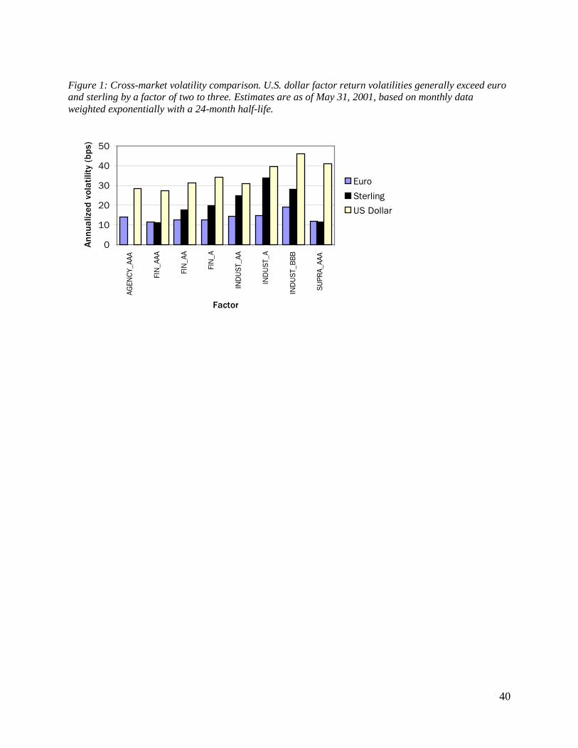
Figure 1 shows a comparison of volatility forecasts as of May 31, 2001 for different factors
common to the euro, sterling, and US dollar markets. These forecasts are computed as standard
deviations in basis points per year based on historical monthly data from the study period that is
exponentially weighted with a 24-month half-life, most recent returns weighted most strongly.
US dollar volatilities are consistently higher than euro or sterling volatilities, frequently by a
factor of two or three. Sterling
volatilities are sometimes closer to US dollar values, other times to euro
values. None of the markets is a good proxy for the others.
10
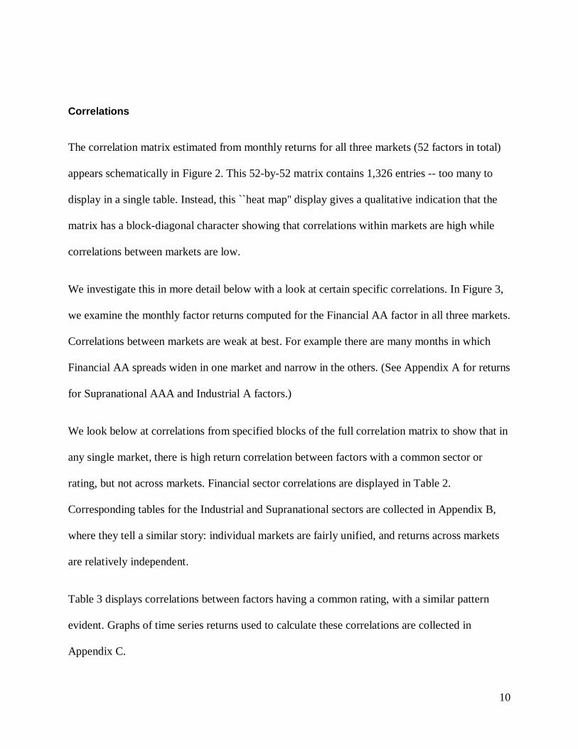
Correlations
The correlation matrix estimated from monthly returns for all three markets (52 factors in total)
appears schematically in Figure 2. This 52-by-52 matrix contains 1,326 entries -- too many to
display in a single table. Instead, this ``heat map'' display gives a qualitative indication that the
matrix has a block-diagonal character showing that correlations within markets are high while
correlations between markets are low.
We investigate this in more detail below with a look at certain specific correlations. In Figure 3,
we examine the monthly factor returns computed for the Financial AA factor in all three markets.
Correlations between markets are weak at best. For example there are many months in which
Financial AA spreads widen in one market and narrow in the others. (See Appendix A for returns
for Supranational AAA and Industrial A factors.)
We look below at correlations from specified blocks of the full correlation matrix to show that in
any single market, there is high return correlation between factors with a common sector or
rating, but not across markets. Financial sector correlations are displayed in Table 2.
Corresponding tables for the Industrial and Supranational sectors are collected in Appendix B,
where they tell a similar story: individual markets are fairly unified, and returns across markets
are relatively independent.
Table 3 displays correlations between factors having a common rating, with a similar pattern
evident. Graphs of time series returns used to calculate these correlations are collected in
Appendix C.

11
Anomalous cross-market correlation
Among the cross-market correlations in the full matrix of Figure 2, we noticed a curiously high
value between euro Utility factors and sterling Industrials. This was striking especially since
correlations between euro Industrials and sterling Industrials were low (See Table 4).
A close examination reveals that these correlations are not a statistical anomaly, but are are a
consequence of the sector classification schemes used in the EuroBIG and EuroSterling indices.
The Utility sector of EuroBIG has a large Telecommunications subsector, but the EuroSterling
index has no Utility sector --- its numerous Telecommunications bonds reside in the Industrial
sector. This inconsistent sector mapping explains the counterintuitive correlations displayed in
Table 4.
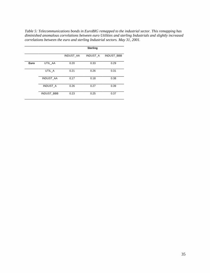
We explored this by remapping the Telecommunications subsector of the EuroBIG Utility sector
to the Industrial sector and then re-estimating the model. The result: the correlations between the
euro Utility sectors and the sterling Industrial sectors dropped while the correlations between the
euro and sterling Industrial sectors increased (see Table 5).
STATISTICAL CONFIDENCE LEVELS
The apparent independence of markets described above invites the question of whether our
conclusions are statistically justified given the amount of data available to estimate our factor
returns. Could our results be simply due to bad luck in the sample?

12
To investigate this, we test the null hypothesis that, for a given factor (say, Financial AA), the
average return in a given month for euro-denominated bonds is equal to the average return for
sterling-denominated bonds. That is, we assume that individual bond returns are independently
drawn from a normal distribution with a common mean across markets, and ask for the
probability, under that assumption, of seeing the data actually observed. To accomplish this, we
compute a t-statistic for each month, and from that we compute a confidence level of rejection of
the null hypothesis. Technically, our null hypothesis requires the use of a weighted t-statistic,
because we assume that an indidividual bond's spread return is drawn from a normal distribution
with variance proportional to the reciprocal of the bond's duration. This leads us to use the
duration-weighted average return as the best unbiased linear estimator of the common mean,
which is how the factor returns were actually calculated in our study (See Appendix D for a
detailed discussion of the weighted t-statistic.)
Figure 4 shows, month by month, the confidence level of rejection of the null hypothesis. That is,
in any month, 100 - (confidence level shown) is the probability that the observed data could have
occurred by chance under the null hypothesis. Confidence levels above 95% indicate that we
may safely assume the null hypothesis fails -- that is, that the mean spread return in each market
is statistically different and therefore they should not be estimated together with a combined set
of bonds).

13
A SEARCH FOR FINANCIAL EXPLANATIONS
We are suggesting that perceived credit risk, as reflected by how average spread levels change, is
currency-dependent. A skeptic might suggest that in fact credit risk changes do not depend on
currency but rather on other factors overlooked by our model, causing us to mis-attribute
differences to currency.
Issuer-level data
For example, we notice that the lists of issuer names in each of our three indices have fairly
small overlap, so the aggregate behavior of spreads in each market might be due to differing
characteristics of the actual issuers in each market. This, however, appears not to be the case, as
spreads for bonds even from the same issuer behave differently in different markets.
To show this, we found issuers active in more than one market and compared spread returns in
each market. Table 6 lists four such issuers with a bond in each currency. In Table 7 we display
the time series correlation of returns for each bond and for the three pairs of markets. Generally
speaking, knowledge of credit spreads for an issuer in one market tells us very little about
spreads for the same issue in another market.
Figure 5 shows this in more detail in the case of Toyota. In the same month, sterling Toyota
spreads might widen at the same time as euro Toyota spreads are narrowing. Clearly, Toyota's
default risk cannot be increasing and decreasing at the same time.

14
Other factors
One still might object that spread differences even for individual issuers can be explained by
non-currency factors missing from the model. However, we were unable to find any factors with
explanatory power.
We examined four possibilities: coupon (which may influence tax-related behavior), duration,
maturity, and amount outstanding (as a proxy for liquidity). Examination of the data shows no
strong trends linking these quantities to spread return. Amount outstanding showed a mild
inverse correlation with spread level, but not spread return. Representative results are shown in
Figure 6 for outstanding bonds as of May 31, 2001 issued by the European Investment Bank.

15
CONCLUSIONS
Our analysis shows that euro, sterling, and US dollar credit spreads have been largely
uncorrelated during our study period of May 1999 to May 2001. Our immediate conclusion is
that credit risk models need to be built separately for the three markets.
Given our findings above for individual issuers, it seems clear that monthly changes in spread-to-
swap levels should not primarily be attributed to changes in perceived creditworthiness of the
issuer. Our view is that credit spread changes in a given market instead primarily reflect changes
in the average risk premium required by investors in that market for a given sector and credit
rating. Causes for these fluctuations will be found in the overall economic and political
conditions that influence investor confidence, and these conditions are somewhat separate for
each of the three markets under study. This explanation is also consistent with our finding of
high spread return correlations across sectors and ratings within a single market.
The failure of covered interest arbitrage to rigidly link credit risk across currencies indicates the
presence of substantial frictions across credit market boundaries. The nature of these frictions
would be an interesting topic for further study.
To the extent that markets become more unified in the future as a result of the globalization of
investment portfolios, our conclusion of currency independence may have to be revised. For
now, credit risk models should respect the tendency of euro, sterling, and US dollar-denominated
credit spreads to go their own ways.

16
Appendix A
Supranational AAA and Industrial A monthly spread returns for the euro, sterlingand U.S. dollar markets
As shown in Figures 7 and 8, there is no significant correlation of Supranational AAA and
Industrial A factors across the euro, sterling, and U.S. dollar markets.
Appendix B
Correlations within and across markets for some sector-defined factors
In the Industrial sector, within-market correlations are high and cross-market correlations are
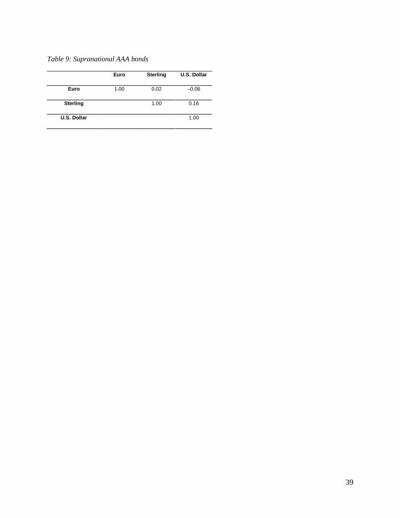
near zero (Tables 8a–d). For Supranational AAA bonds, cross-market correlations are near zero
(Table 9).
Appendix C
AA credit spread returns
Time-series analyses of AA credit spread returns for the euro, sterling and U.S. dollar markets
show that, within each market and rating class, there are strong correlations across sectors
(Figures 9a–c).

17
Appendix D
t-statistics for weighted means with application to risk factor models
In this appendix we describe how to generalize the standard t-statistic test for equality of the
means when the assumption of a common variance no longer holds. We derive a formula for the
generalized t-statistic (equation 3 below), which was used to compute the confidence levels
reported in Figure 4. First, we describe the standard t-statistic. Suppose we have a sequence of
independent samples from a normal distribution with mean µX and variance s2. Denote the
sample values by X1, X2,...,Xn. We use the notation Xi~N(µX,s2), where N(a, b) denotes the
probability density function of a normal distribution with mean a and variance b.
The best (minimum variance) linear unbiased estimator of the mean µ is the sample mean
If Y1 ,Y2 ,...,Ym is another group of independent samples with Yi~N(µY,s2), we could ask whether
or not µX = µY . We take the null hypothesis to be the statement that this equality is true.
Given our sample data, we cannot determine the truth or falsity of the null hypothesis, but we
can determine the likelihood of the realized sample values assuming the null hypothesis. If this
likelihood is small, we are justified in rejecting the null hypothesis.
To accomplish this, we may use the standard (Student’s) t-statistic for equality of the mean:
(1)

18
where
is the sample variance of X, and similarly for Y.
The random variable T has a t-distribution with n + m–2 degrees of freedom. Therefore, we can
determine the probability that T is equal to or greater than the realized value, given µX = µY.
Typically, if this probability is below 5% or 1%, the null hypothesis is rejected.
In this paper we generalize the discussion to the case where the samples are drawn from
distributions with a common mean but variances allowed to change from sample to sample:
In this case, the best linear unbiased estimate of the mean µX is the weighted average
(2)
where
Conversely, given positive weights wi, i =1,...,n so that ,then the quantity in equation 2 is the best

19
linear unbiased estimate of the mean provided that the samples are distributed as
for some constant aX > 0.
In either case, if
is the weighted sample variance, and if we use similar notation for Yi (with different weights w¢i
allowed), then the corresponding formula for the t-statistic for equality of the weighted mean is
(3)
Setting wi =1/n, wi =1/m, and aY =(n/m)aX reduces this expression to equation 1.
Note: T is independent of the scale of the pair (aX,aY ): if (aX,aY )is replaced by (kaX,kaY ) for
some k >0, the value of T is unchanged.
The weighted mean as a minimum variance estimator
If X1,X2,...,Xn is a random sample such that Xi~N(µ,si2 ), what is the minimum variance unbiased
estimator of the mean? It is a weighted sum where greater weight is given to values coming from
narrower distributions.

20
Let Xi = µ + ei where ei has mean 0 and variance si2. If
is to be the minimum variance unbiased estimator of the mean µ , then we must solve for the
weights wi, minimizing the variance of X, subject to the constraint
(4)
Because we are assuming that the variables ei are independent, we have
The method of Lagrange multipliers to minimize this function subject to the constraint in
equation 4 yields
We obtain this weight if we set

21
where a is any positive constant. This proves
Proposition 1 Let a be a positive constant. Suppose w1,...,wn are positive numbers satisfying Σwi
=1, and, for each i, Xi is a random variable with mean µ and variance a/wi.
Then the minimum variance unbiased estimator of the mean µ is
Establishing the weighted t-statistic
Recall that if a random variable V is the sum of the squares of r > 0 independent standard normal
variables, then V is said to have a chi-squared distribution with r degrees of freedom.
The t-distribution with r degrees of freedom may be defined as the distribution of the random
variable
where W is a standard normal random variable, V has a chi-squared distribution with r degrees of
freedom, and W and V are independent.
We need to show that the statistic defined in equation 3 has a t-distribution with n + m–2 degrees
of freedom. We accomplish this with a sequence of lemmas in this section.
Standing assumptions: Let aX and aY be fixed positive numbers. For i =1,...,n, and j =1,...,m, let

22
wi and w¢j be positive numbers and Xi, Yj independent random variables such that
• and
and
• for each i, j, and .
Notation:
• and
• and
Lemma 1:
Proof. A straightforward computation using the fact that a sum of independent normals is normal
and variances add.
Lemma 2:
X(mean), Y(mean), SX, and SY are mutually independent.
Proof. Clearly X(mean) and Y(mean) are independent, and similarly for SX and SY .We show that
X(mean) is independent of SX , and the same argument works for SY. The argument is a direct

23
generalization of the proof for the equal weighted case found, for example, in Hogg and Craig
(1995), which we include here for the reader’s convenience.
Write a = aX and denote the variance of Xi by si2 (=a/wi). The joint probability density function
(pdf) of X1, X2,..., Xn is
Our strategy is to change variables in such a way that the independence of X(mean) and SX will
be evident. Letting x(mean) = Swixi, straightforward computation verifies that
and
(5)
Hence
(6)
Consider the linear transformation (u1,...,un)=L(x1,...,xn) defined by u1 = x(mean), u2 = x2 –
x(mean),...,un = xn– x(mean), with inverse transformation

24
Likewise define new random variables U1 = X(mean), U2 = X2 – X(mean),..., Un =Xn – X(mean).
If J denotes the Jacobian of L, then the joint pdf of U1,..., Un is
This now factors as a product of the pdf of U1 and the joint pdf of U2,..., Un. Hence U1 =
X(mean) is independent of U2,..., Un, and hence also independent of
Lemma 3:
SX /aX ~c2(n–1) and SY /aY ~ c2(m–1), where c2(k) denotes the chi-squared distribution with k
degrees of freedom.
Proof. The proofs for X and Y are similar. Let

25
and
Then by equation 5, A = B + C. Since Xi ~N(mX,si2 ), A~c2(n). Similarly C~c2(1). This implies
that B = SX /aX ~c2(n–1) provided that B and C are independent, which follows from the proof of
lemma 2.
Proposition 2
is a t-statistic with n + m–2 degrees of freedom.
Proof. Let
and

26
By Lemma 2, W and V are independent. From Lemma 1, W is a standard normal random
variable. From Lemma 3, V~c2(n + m–2). Hence
has the required property.
Application to risk modeling
For certain financial risk factor models, the return to a given factor is computed as the weighted
average of returns to the individual securities exposed to that factor. For example, a model for
bond credit risk may have a Financial factor to which all financial bonds rated AA are exposed.
If the return to this factor is defined to be the duration-weighted average of the option adjusted
spread (OAS) returns Xi , we would take weights
where Di is the duration of the ith bond. The factor return is then the weighted average
We may interpret this factor return as the best linear unbiased estimator of the common mean of
a set of independent normal distributions from which the individual bond OAS returns are
27
sampled; the distributions are those of Proposition 1.
If, in the course of building the model, the question arises whether two groups of bond OAS
returns X1 ,X2 ,...,Xn and Y1 ,Y2 ,...,Ym share the same mean and therefore should be exposed to the
same risk factor, we may use the t-statistic of equation 3 to examine the question. A large value
of this statistic is evidence that the two groups of bonds have different means and therefore
should be exposed to separate risk factors.
Acknowledgements
The authors thank Tim Backshall, Oren Cheyette, Anton Honikman, and Darren Stovel for
insightful discussions and comments on the manuscript, and Tim Tomaich for help with the U.S.
dollar credit model. Special thanks to Justine Withers for a fabulous editing job.
Notes
1- Factors are:
1 EUR_FIN_AAA
2 EUR_FIN_AA
3 EUR_FIN_A
4 EUR_SOV_AA
5 EUR_SOV_A
6 EUR_AGENCY_AAA
7 EUR_UTIL_AA
8 EUR_UTIL_A
9 EUR_UTIL_BBB
10 EUR_ INDUST_AA
11 EUR_ INDUST_A
12 EUR_ INDUST_BBB
13 EUR_ PFAND_AAA
14 EUR_ SUPRA_AAA
15 GBP_FIN_AAA
16 GBP_FIN_AA
17 GBP_FIN_A
18 GBP_INDUST_AA
19 GBP_INDUST_A
20 GBP_INDUST_BBB
21 GBP_SOV_AAA
22 GBP_SOV_AA
23 GBP_SUPRA_AAA
24 GBP_AGENCY
25 USD_CANADIAN_AA
26 USD_CANADIAN_A
27 USD_CANADIAN_BBB
28 USD_ENERGY_AA
29 USD_ENERGY_A
30 USD_ENERGY_BBB
31 USD_FINANCIAL_AAA
32 USD_FINANCIAL_AA
33 USD_FINANCIAL_A
34 USD_FINANCIAL_BBB
35 USD_ INDUST_AAA
36 USD_INDUST_AA
37 USD_ INDUST_A
38 USD_INDUST_BBB
39 USD_UTILITY_AA
40 USD_UTILITY_A
41 USD_SUPRANTL_AAA
42 USD_TRANSPORT_AA
43 USD_TRANSPORT_A
44 USD_TRANSPORT_BBB
45 USD_TELE_AA
46 USD_TELE_A
48 USD_TELE_BBB
49 USD_YANKEE_AAA
50 USD_YANKEE_AA
51 USD_YANKEE_A
52 USD_YANKEE_BBB

28
2- These observations do not extend to bonds that are below investment grade. Empiricalevidence shows that in the U.S. market, there is little correlation between below andabove investment grade bonds in the same sector.
3- The Utility BBB sector is missing in the remapped model since virtually all the EuroBIGBBB Utility bonds were in the Telecommunications subsector.

29
References
Hogg, R. V. and A. T. Craig. “Introduction to Mathematical Statistics.” 5th edition. UpperSaddle River, New Jersey: Prentice-Hall, 1995.
Merrill Lynch. “Merrill Lynch Global Bond Indices, Rules of Construction and CalculationMethodology”. 2000.
O’Kane, D. “Credit Derivatives Explained.” Lehman Brothers, 2000.
Salomon Smith Barney. “Performance Indexes”. 1999, pp. 41-46.

30
TABLES & FIGURES
Table 1: The number of bonds available in each sector-by-rating bucket on May 31, 2001.
AAA AA A BBB
Euro Agency 96 24
Financial 44 56 33
Industrial 9 46 17
Sovereign 4 8 5
Supranational 26
Utility 10 32 11
Pfandbrief 184
Sterling Financial 17 36 13
Industrial 7 55 19
Sovereign 14 12
Supranational 32
U.S.Dollar
Canadian 18 66 61
Supranational 26
Transportation 7 15 72
Utility 7 91 127
Energy 9 17 134
Telecommunications
55 76 33
Industrial 13 57 310 375
Yankee 11 28 79 124
Financial 29 168 527 147
Agency 268

31
Tables 2a–d: Financial sector correlations within and across markets as of May 31, 2001. Most within-market correlations are close to one and cross-market correlations are closer to zero. Correlationsbetween sterling and U.S. dollar sectors tend to be stronger than correlations between euro sectors andsectors in other markets.
Table 2a: Correlations between euro Financial sectors.
FIN_AAA FIN_AA FIN_A
FIN_AAA 1.00 0.850 0.76
FIN_AA 1.00 0.86
FIN_A 1.00
Table 2b: Correlations between sterling Financial sectors.
FIN_AAA FIN_AA FIN_A
FIN_AAA 1.00 0.61 0.65
FIN_AA 1.00 0.96
FIN_A 1.00
Table 2c: Correlations between U.S. dollar Financial sectors.
FIN_AAA FIN_AA FIN_A FIN_BBB
FIN_AAA 1.00 0.77 0.66 0.73
FIN_AA 1.00 0.94 0.91
FIN_A 1.00 0.91
FIN_BBB 1.00

32
Table 2d: Cross-market Financial sector correlations.
FIN_AAA FIN_AA FIN_A
Euro/sterling 0.10 –0.18 –0.06
Euro/U.S. dollar 0.11 –0.06 –0.05
Sterling/U.S. dollar 0.12 0.44 0.51

33
Tables 3a–d: Correlations within markets and across markets for AA factors. May 31, 2001.
Table 3a: Correlations between euro AA sectors.
FIN_AA SOV_AA UTIL_AA INDUST_AA
FIN_AA 1.00 0.82 0.56 0.73
SOV_AA 1.00 0.27 0.67
UTIL_AA 1.00 0.61
INDUST_AA 1.00
Table 3b: Correlations between sterling AA sectors.
FIN_AA INDUST_AA
FIN_AA 1.00 0.87
INDUST_AA 1.00
Table 3c: Correlations between U.S. dollar AA sectors.
CANADIAN_AAENERGY_AA FIN_AA INDUST_AAUTIL_AATRANSPORT_AATELE_AAYANKEE_AA
CANADIAN_AA 1.00 0.52 0.67 0.80 0.75 0.47 0.82 0.59
ENERGY_AA 1.00 0.41 0.63 0.80 0.80 0.74 0.55
FIN_AA 1.00 0387 0.60 0.45 0.75 0.79
INDUST_AA 1.00 0.79 0.57 0.86 0.72
UTIL_AA 1.00 0.71 0.94 0.60
TRANSPORT_AA 1.00 0.63 0.64
TELE_AA 1.00 0.72
YANKEE_AA 1.00
Table 3d: Cross-market correlations between AA sectors.
FIN_AA INDUST_AA UTILITY_AA
Euro/sterling –0.18 –0.12
Euro/U.S. dollar –0.06 –0.02 –0.05
Sterling/U.S. dollar 0.44 0.06

34
Table 4: Relatively high correlations between euro Utilities and sterling Industrials, near zerocorrelations between euro Industrials and sterling Industrials. May 31, 2001.
Sterling
INDUST_AA INDUST_A INDUST_BBB
Euro UTIL_AA 0.35 0.33 0.52
UTIL_A 0.32 0.36 0.47
UTIL_BBB 0.47 0.51 0.56
INDUST_AA –0.12 –0.06 0.02
INDUST_A 0.12 0.12 0.23
INDUST_BBB –0.22 –0.25 –0.07
35
Table 5: Telecommunications bonds in EuroBIG remapped to the industrial sector. This remapping hasdiminished anomalous correlations between euro Utilities and sterling Industrials and slightly increasedcorrelations between the euro and sterling Industrial sectors. May 31, 2001.
Sterling
INDUST_AA INDUST_A INDUST_BBB
Euro UTIL_AA 0.20 0.33 0.29
UTIL_A 0.21 0.26 0.31
INDUST_AA 0,17 0.18 0.38
INDUST_A 0.26 0.27 0.39
INDUST_BBB 0.23 0.25 0.37

36
Table 6: Examples of bonds issued by the same entity but on different markets.
Issuer Euro Bond Sterling Bond U.S. Dollar Bond
Name Sector Maturity Coupon(%)
Maturity Coupon(%)
Maturity Coupon(%)
Government of CanadaSOV/CAN 2008/07/07 4.875 2004/11/26 6.25 2002/07/15 6.125
Dresdner Bank FIN 2005/05/25 5.0 2007/12/07 7.75 2005/09/15 6.625
European InvestmentBank
SUPRA 2007/02/15 5.75 2003/06/10 8.0 2002/06/01 9.125
Toyota INDUST 2003/11/10 4.75 2007/12/07 6.25 2003/11/13 5.625

37
Table 7: Examples of cross-market correlations for individual issuers. Correlations were computed usingthe bonds given in Table 6.
Issuer Euro/SterlingCorrelation
Euro/U.S. DollarCorrelation
Sterling/U.S. DollarCorrelation
Government of Canada 0.12 –0.10 0.07
Dresdner Bank –0.51 –0.01 –0.03
European Investment Bank 0.17 –0.08 0.01
Toyota –0.21 –0.19 0.23

38
Table 8a: Euro market
INDUST_AA INDUST_A INDUST_BBB
INDUST_AA 1.00 0.60 0.41
INDUST_A 1.00 0.67
INDUST_BBB 1.00
Table 8b: Sterling market
INDUST_AA INDUST_A INDUST_BBB
INDUST_AA 1.00 0.88 0.88
INDUST_A 1.00 0.82
INDUST_BBB 1.00
Table 8c: U.S. dollar market
INDUST_AAA INDUST_AA INDUST_A INDUST_BBB
INDUST_AAA 1.00 0.87 0.78 0.78
INDUST_AA 1.00 0.91 0.87
INDUST_A 1.00 0.96
INDUST_BBB 1.00
Table 8d: Across markets
INDUST_AA INDUST_A INDUST_BBB
Euro/Sterling –0.12 0.12 –0.07
Euro/U.S. Dollar –0.02 0.13 0.21
Sterling/U.S. Dollar 0.06 0.19 0.17
39
Table 9: Supranational AAA bonds
Euro Sterling U.S. Dollar
Euro 1.00 0.02 –0.06
Sterling 1.00 0.16
U.S. Dollar 1.00
40
Figure 1: Cross-market volatility comparison. U.S. dollar factor return volatilities generally exceed euroand sterling by a factor of two to three. Estimates are as of May 31, 2001, based on monthly dataweighted exponentially with a 24-month half-life.
0
10
20
30
40
50
AGEN
CY_
AAA
FIN
_AAA
FIN
_AA
FIN
_A
IND
UST_
AA
IND
UST_
A
IND
UST_
BBB
SU
PRA_
AAA
Factor
Ann
ualiz
ed v
olat
ility
(bp
s)
Euro
Sterling
US Dollar

41
Figure 2: Color-coded map of spread return correlations for the euro, sterling, and U.S. dollar markets.High correlations (0.7–1.0) are consistently observed within a single market, whereas cross-marketcorrelations remain mostly between –0.3 and 0.3. On average, the correlation matrix shows a clearcross-market de-correlation1.

42
Figure 3: Cross-market comparison of Financial AA spread factor returns. Top: return time series.Bottom, left to right: sterling returns plotted as a function of euro returns, and U.S. dollar returns plottedas a function of euro and sterling returns. The corresponding correlations are –0.15, –0.05, and +0.45respectively.
-25
-20
-15
-10
-5
0
5
10
15
20
05/2
8/9
9
07/3
0/9
9
09/3
0/9
9
11/3
0/9
9
01/3
1/0
0
03/3
1/0
0
05/3
1/0
0
07/3
1/0
0
09/2
9/0
0
11/3
0/0
0
01/3
1/0
1
03/3
0/0
1
05/3
1/0
1
Return date
Spr
ead
retu
rn (
bps)
Euro
Sterling
US dollar
-15
-10
-5
0
5
10
15
-10 -5 0 5 10
Euro return (bps)
Ste
rlin
g re
turn
(bp
s)
-30
-20
-10
0
10
20
-10 -5 0 5 10
Euro return (bps)
U.S
. dol
lar
retu
rn (
bps)
-30
-20
-10
0
10
20
-15 -5 5 15
Sterling return (bps)
U.S
. dol
lar
retu
rn (
bps)

43
Figures 4a–b: Confidence levels of rejection of the null hypothesis that the mean returns to a credit factorare the same across currencies. In most cases, returns are shown to have different means. Top:Supranational AAA. Middle: Financial AA. Bottom: Industrial A.
Figure 4a: Euro versus sterling
Supranational AAA
0255075
100
Financial AA
0255075
100
Industrial A
0255075
100
May
-99
Jul-9
9
Sep
-99
Nov
-99
Jan-
00
Mar
-00
May
-00
Jul-0
0
Sep
-00
Nov
-00
Jan-
01
Mar
-01
May
-01
Date
Figure 4b: Euro versus U.S. dollar
Supranational AAA
0255075
100

44
Financial AA
0255075
100
Con
fiden
ce (
%)
Industrial A
0255075
100
May
-99
Jul-9
9
Sep
-99
Nov
-99
Jan-
00
Mar
-00
May
-00
Jul-0
0
Sep
-00
Nov
-00
Jan-
01
Mar
-01
May
-01
Date

45
Figure 5: Cross-market comparison of spread returns for three bonds issued on different markets byToyota. The cross-market correlations corresponding to the bottom panels are, from left to right, –0.21, –0.19, and 0.23.
-20
-15
-10
-5
0
5
10
15
20
Jan-
00
Mar
-00
May
-00
Jul-0
0
Sep
-00
Nov
-00
Jan-
01
Mar
-01
May
-01
Date
Spr
ead
retu
rn (
bps)
Euro
Sterling
US dollar
-15
-10
-5
0
5
10
15
-20 -10 0 10
Euro return (bps)
Ste
rlin
g re
turn
(bp
s)
-25-20-15-10-505
1015
-20 -10 0 10
Euro return (bps)
U.S
. dol
lar
retu
rn (
bps)
-25-20-15-10-505
1015
-20 -10 0 10 20
Sterling return (bps)
U.S
. dol
lar
retu
rn (
bps)

46
Figure 6: Spread returns of bonds issued by the European Investment Bank on the euro, sterling, and U.S.dollar markets plotted as a function of amount outstanding, maturity, duration, and coupon. There is noclear relation between either of these factors and the returns.
-10
-5
0
5
10
15
20
0 2000 4000 6000
Amount outstanding (millions)
Spr
ead
retu
rn (
bps)
-10
-5
0
5
10
15
20
2000 2005 2010 2015 2020
Maturity (years)
-10
-5
0
5
10
15
20
0 5 10 15 20
Duration
Spr
ead
retu
rn (
bps)
-10
-5
0
5
10
15
20
0 2 4 6 8 10
Coupon (%)

47
Figure 7: Cross-market comparison of Supranational AAA spread factor returns. Top: return time series.Bottom, from left to right: sterling returns plotted as a function of euro returns, and U.S. dollars returnsplotted as a function of euro and sterling returns. The corresponding correlations are 0.026, -0.083, and0.23 respectively. Supranational AAA spread returns appear to be relatively independent across the euro,sterling and U.S. dollar markets.
-30
-20
-10
0
10
20
30
05/2
8/9
9
07/3
0/9
9
09/3
0/9
9
11/3
0/9
9
01/3
1/0
0
03/3
1/0
0
05/3
1/0
0
07/3
1/0
0
09/2
9/0
0
11/3
0/0
0
01/3
1/0
1
03/3
0/0
1
05/3
1/0
1Return date
Spr
ead
retu
rn (
bps)
Euro
Sterling
US dollar
-10
-5
0
5
10
-10 -5 0 5 10
Euro return (bps)
Ster
ling
retu
rn (
bps)
-30
-20
-10
0
10
20
30
-10 -5 0 5 10
Euro return (bps)
U.S
. dol
lar
retu
rn (
bps)
-30
-20
-10
0
10
20
30
-10 -5 0 5 10
Sterling return (bps)
U.S
. dol
lar
retu
rn (
bps)

48
Figure 8: Cross-market comparison of Industrial A spread factor returns. Top: return time series.Bottom, from left to right: sterling returns plotted as a function of euro returns, and U.S. dollar returnsplotted as a function of euro and sterling returns. The corresponding correlations are 0.12, 0.17, and0.20 respectively. Note, again, the independence of spread returns across markets.
-30
-20
-10
0
10
20
30
05/2
8/9
9
07/3
0/9
9
09/3
0/9
9
11/3
0/9
9
01/3
1/0
0
03/3
1/0
0
05/3
1/0
0
07/3
1/0
0
09/2
9/0
0
11/3
0/0
0
01/3
1/0
1
03/3
0/0
1
05/3
1/0
1
Return date
Spr
ead
retu
rn (
bps)
Euro
Sterling
US dollar
-30
-20
-10
0
10
20
30
-10 -5 0 5 10
Euro return (bps)
Ste
rlin
g re
turn
(bp
s)
-30
-20
-10
0
10
20
30
-10 -5 0 5 10
Euro return (bps)
U.S
. dol
lar
retu
rn (
bps)
-30
-20
-10
0
10
20
30
-30 -20 -10 0 10 20 30
Sterling return (bps)
U.S
. dol
lar
retu
rn (
bps)

49
Figure 9a: Euro AA credit spread returns
-10
-5
0
5
10
15
2/9
/99
5/2
0/9
9
8/2
8/9
9
12/6
/99
3/1
5/0
0
6/2
3/0
0
10/1
/00
1/9
/01
4/1
9/0
1
7/2
8/0
1
Date
Bas
is P
oint
s FIN_AA
SOV_AA
UTIL_AA
INDUST_AA

50
Figure 9b: U.S. dollar AA credit spread returns
-60
-50
-40
-30
-20
-10
0
10
20
30
40
2/9
/99
5/2
0/9
9
8/2
8/9
9
12/6
/99
3/1
5/0
0
6/2
3/0
0
10/1
/00
1/9
/01
4/1
9/0
1
7/2
8/0
1Date
Bas
is P
oint
s
CANADIAN_AA
ENERGY_AA
FINANCIAL_AA
INDUST_AA
UTILITY_AA
TRANSPORT_AA
TELE_AA
YANKEE_AA

51
Figure 9c: Sterling AA credit spread returns
-20
-10
0
10
20
30
2/9
/99
5/2
0/9
9
8/2
8/9
9
12/6
/99
3/1
5/0
0
6/2
3/0
0
10/1
/00
1/9
/01
4/1
9/0
1
7/2
8/0
1
Date
Bas
is P
oint
s
FIN_AA
INDUST_AA