Rene Magritte

10/18/07

Modeling Cochlear Dynamics

Christopher Bergevin

Department of Mathematics

University of Arizona

Disclaimer:

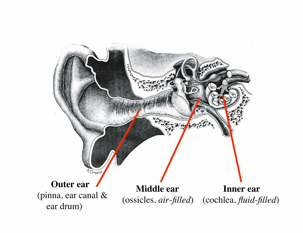
Inner ear (cochlea, fluid-filled)

Middle ear (ossicles, air-filled)

Outer ear(pinna, ear canal & ear drum)

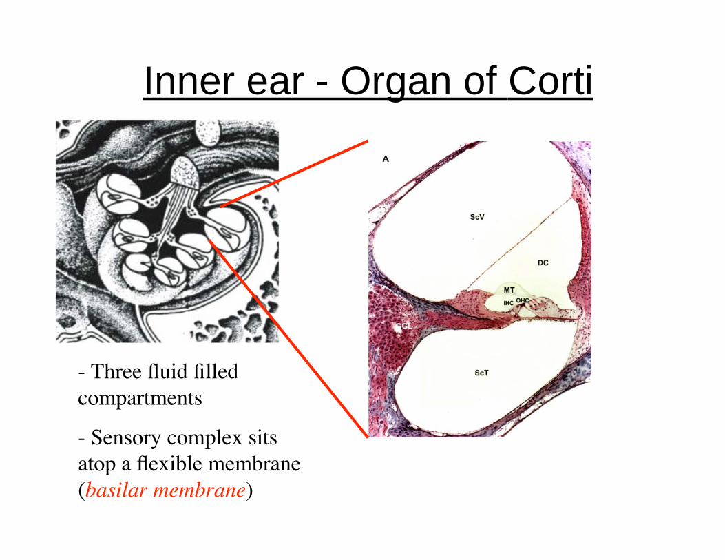
Inner ear - Organ of Corti

- Three fluid filledcompartments

- Sensory complex sitsatop a flexible membrane(basilar membrane)

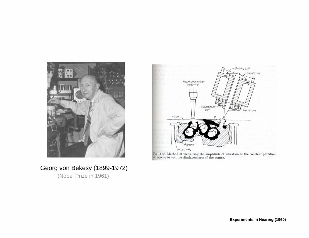
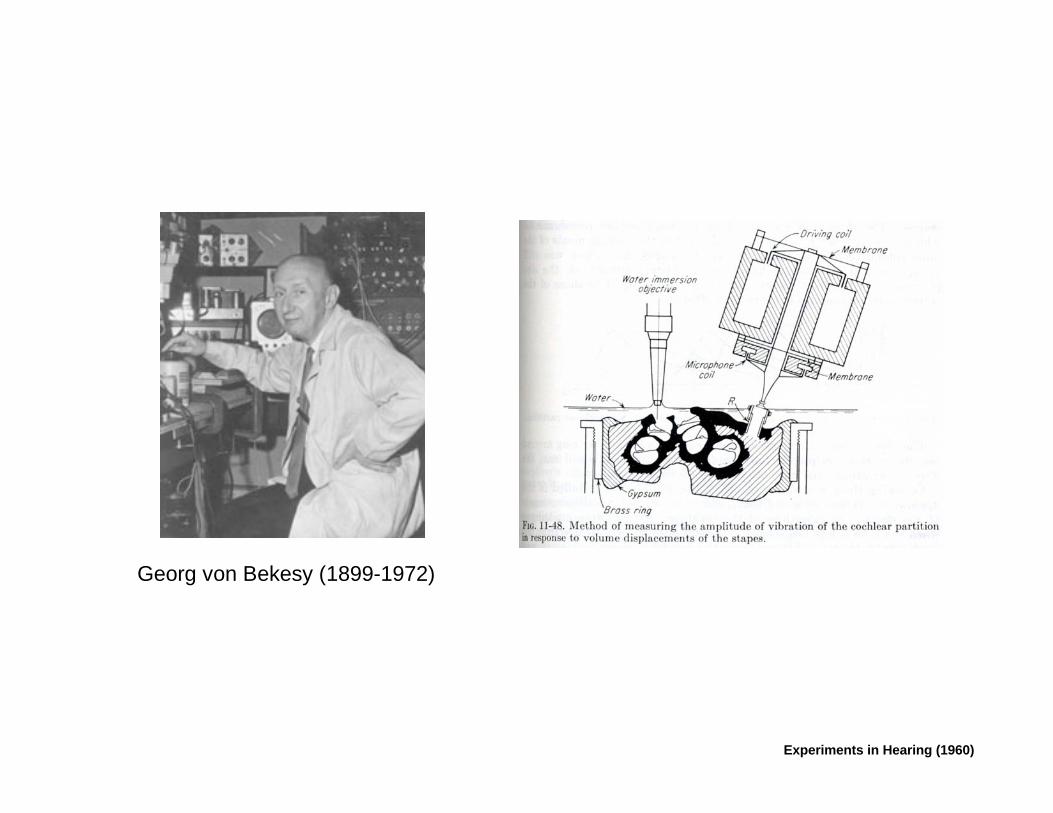
Experiments in Hearing (1960)

Georg von Bekesy (1899-1972)

(Nobel Prize in 1961)

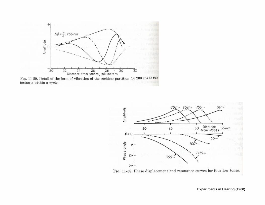
Experiments in Hearing (1960)

Question: Can we develop a model based upon

the anatomy that captures the observed

physiological features?

Goal: Model should serve as a foundation

1-D transmission-line model solved using WKB approximation

Assumptions

- height of traveling wave is small relative to the

height of the scalae (pressure is uniform in both cross-sections and depends only upon longitudinal distance)

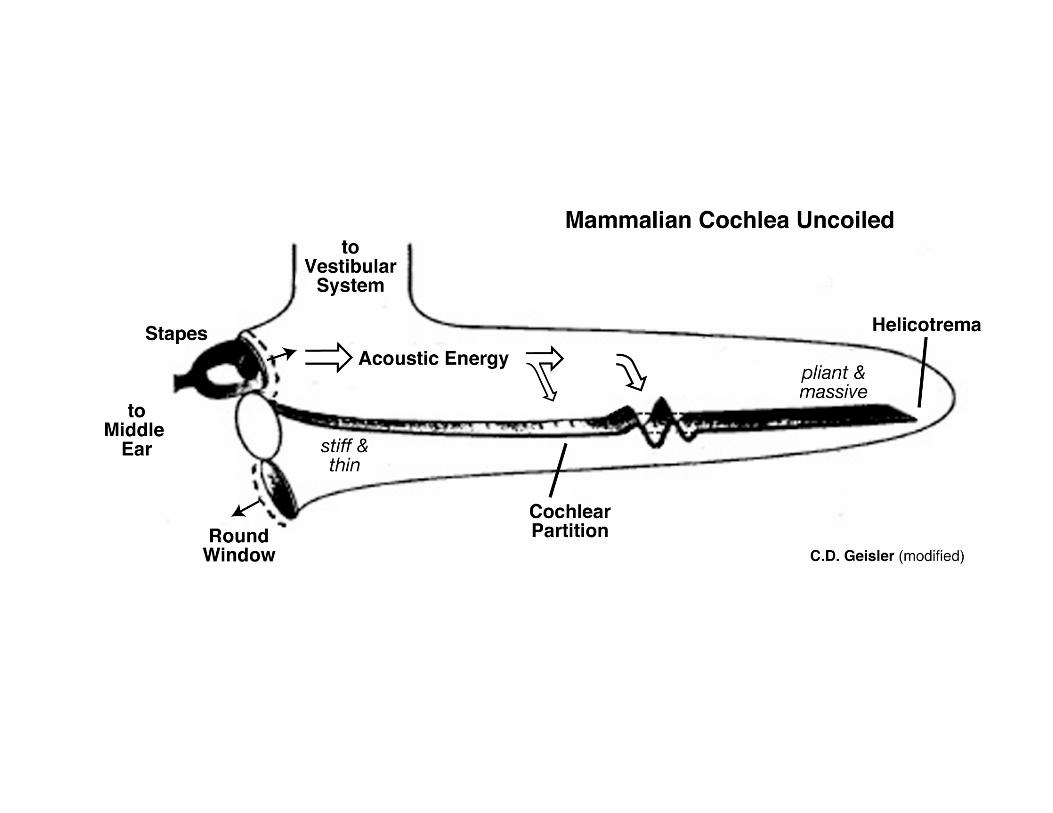
- effect of coiling is negligible (allows us to ‘unroll’ the cochlea)

- fluid is incompressible and viscosity negligible

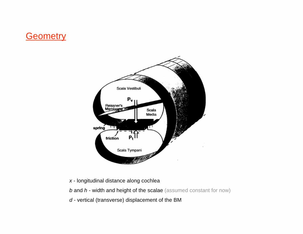
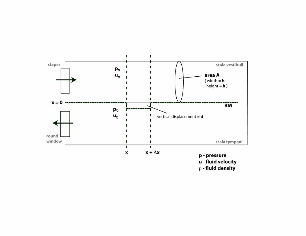
Geometry

x - longitudinal distance along cochlea

b and h - width and height of the scalae (assumed constant for now)

d - vertical (transverse) displacement of the BM

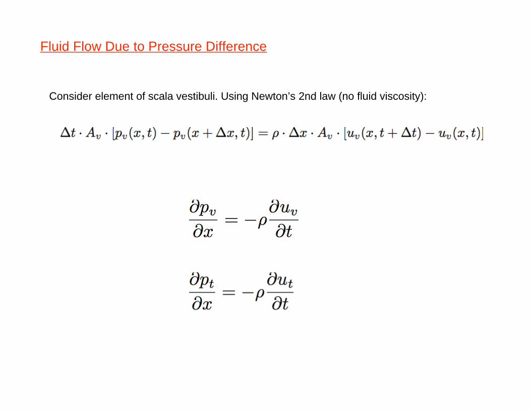
Fluid Flow Due to Pressure Difference

Consider element of scala vestibuli. Using Newton’s 2nd law (no fluid viscosity):

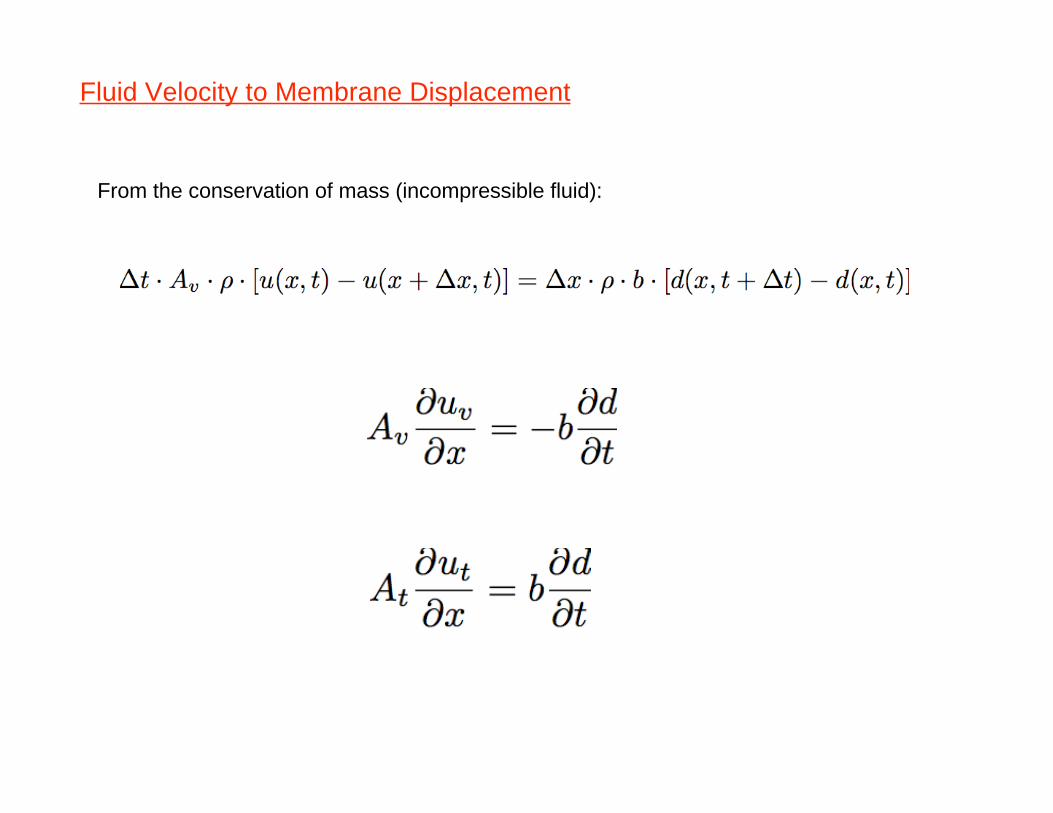
Fluid Velocity to Membrane Displacement

From the conservation of mass (incompressible fluid):

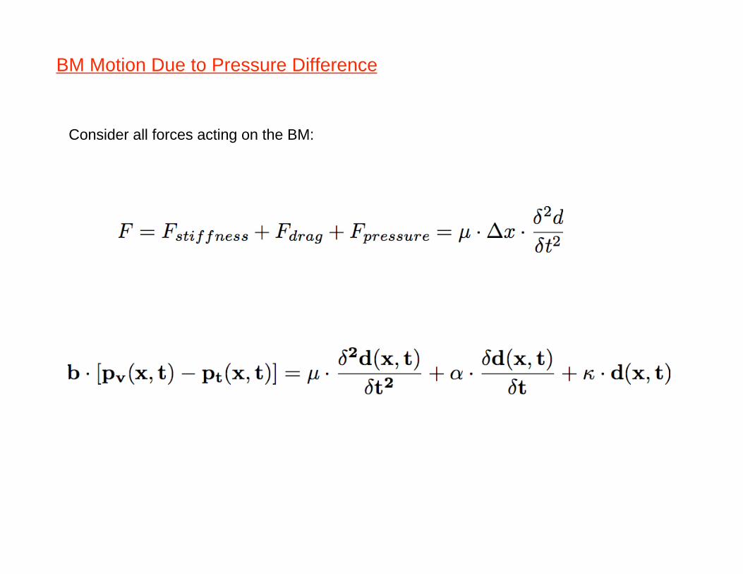
BM Motion Due to Pressure Difference

Consider all forces acting on the BM:

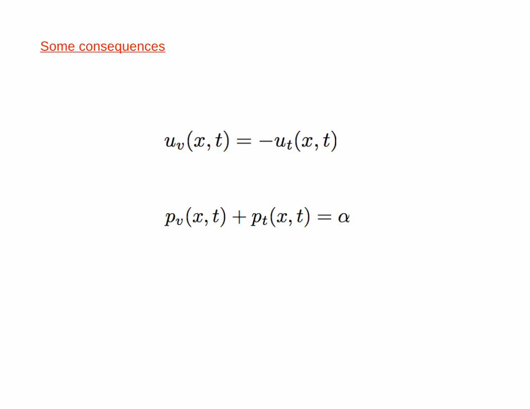
Some consequences

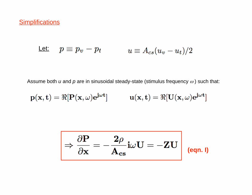
Simplifications

Let:

Assume both u and p are in sinusoidal steady-state (stimulus frequency ) such that:

(eqn. I)

Simplifications II

Plugging back into the equation of motion (relating pressure and displacement):

(eqn. II)

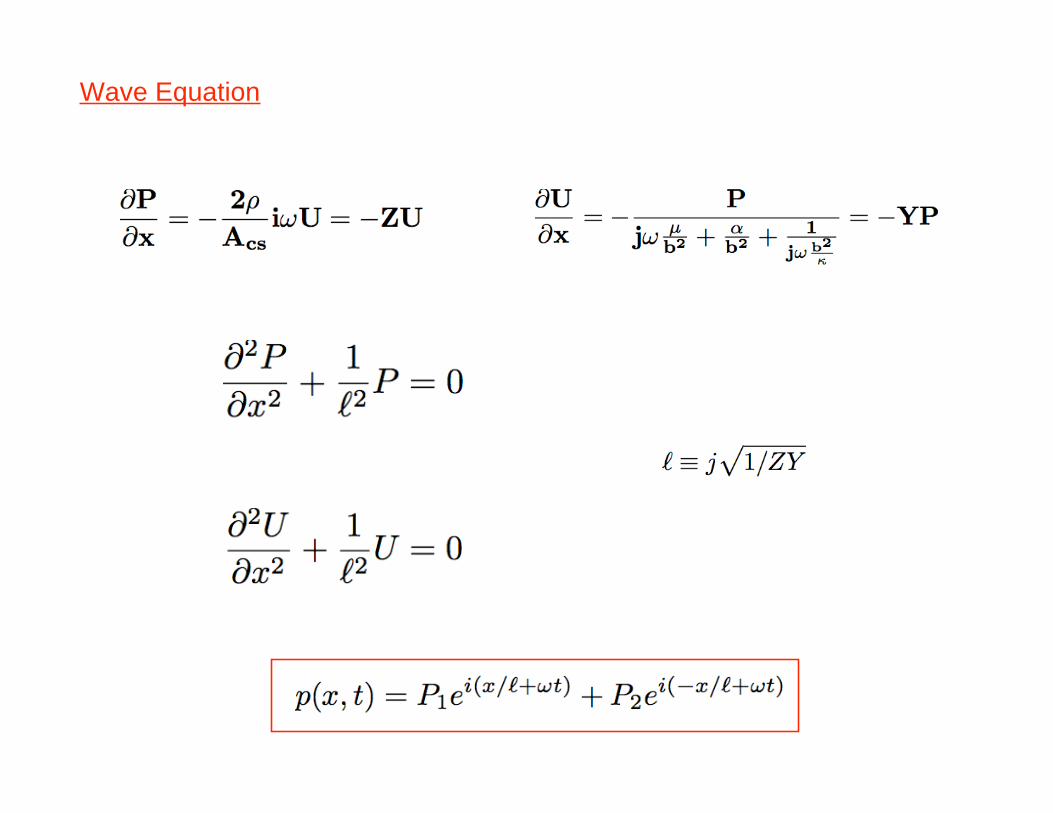
Wave Equation

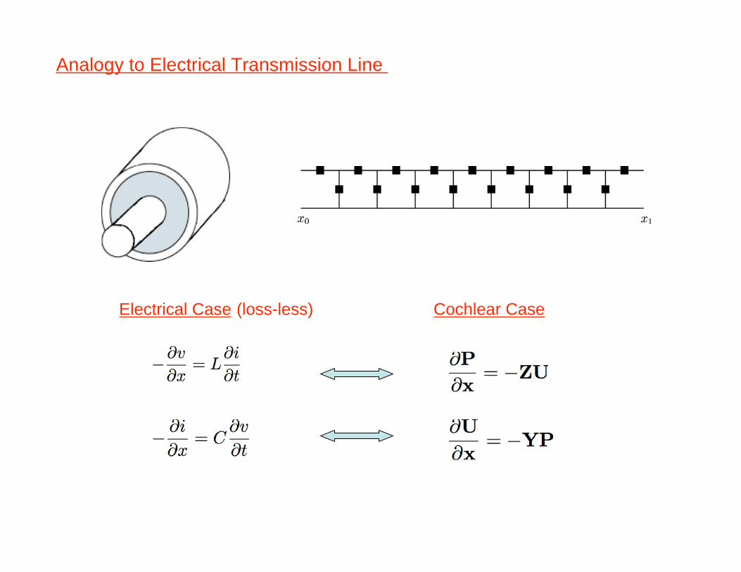
Analogy to Electrical Transmission Line

Electrical Case (loss-less) Cochlear Case

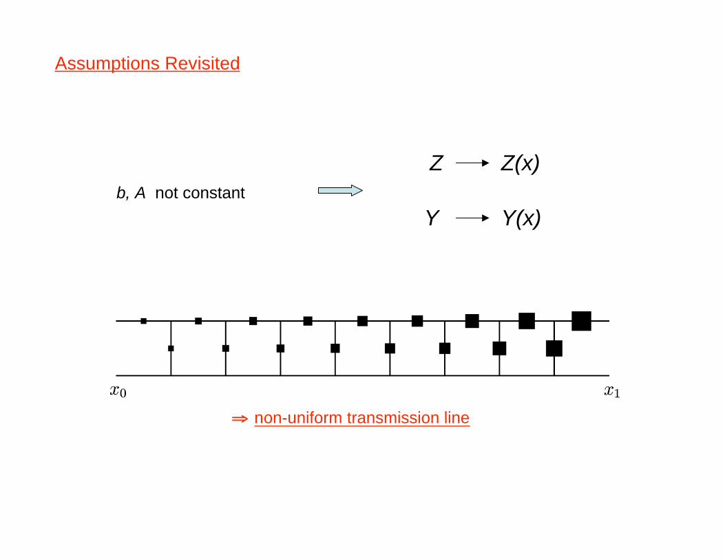
Assumptions Revisited

non-uniform transmission line

b, A not constant

Z

Y Y(x)

Z(x)

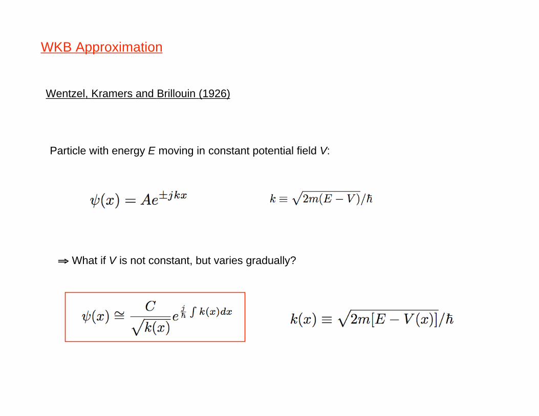
WKB Approximation

Wentzel, Kramers and Brillouin (1926)

Particle with energy E moving in constant potential field V:

What if V is not constant, but varies gradually?

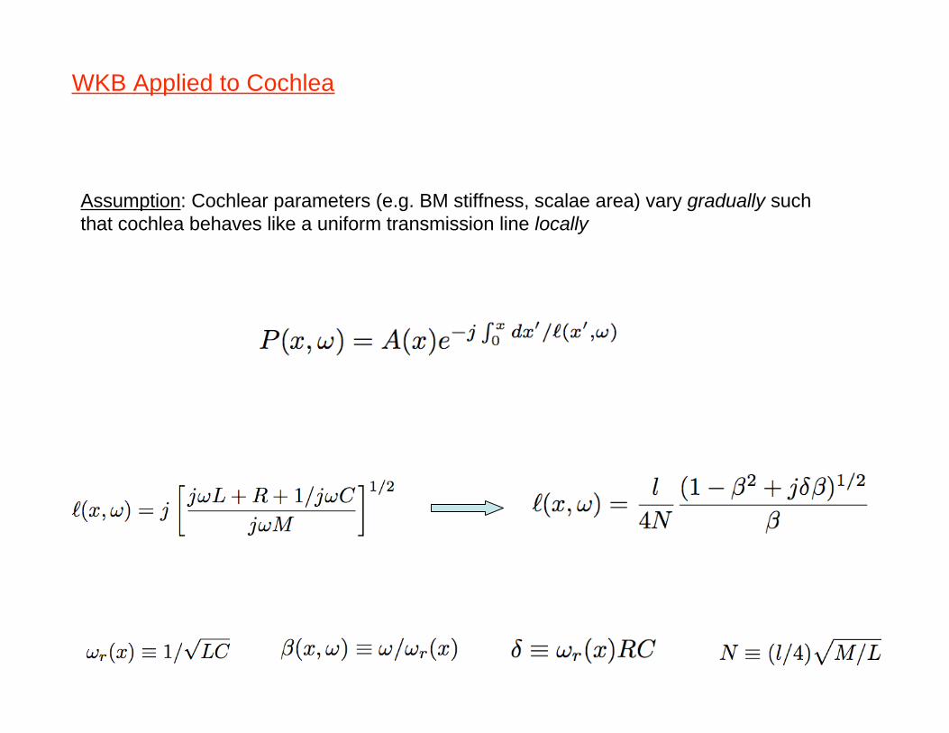
WKB Applied to Cochlea

Assumption: Cochlear parameters (e.g. BM stiffness, scalae area) vary gradually such

that cochlea behaves like a uniform transmission line locally

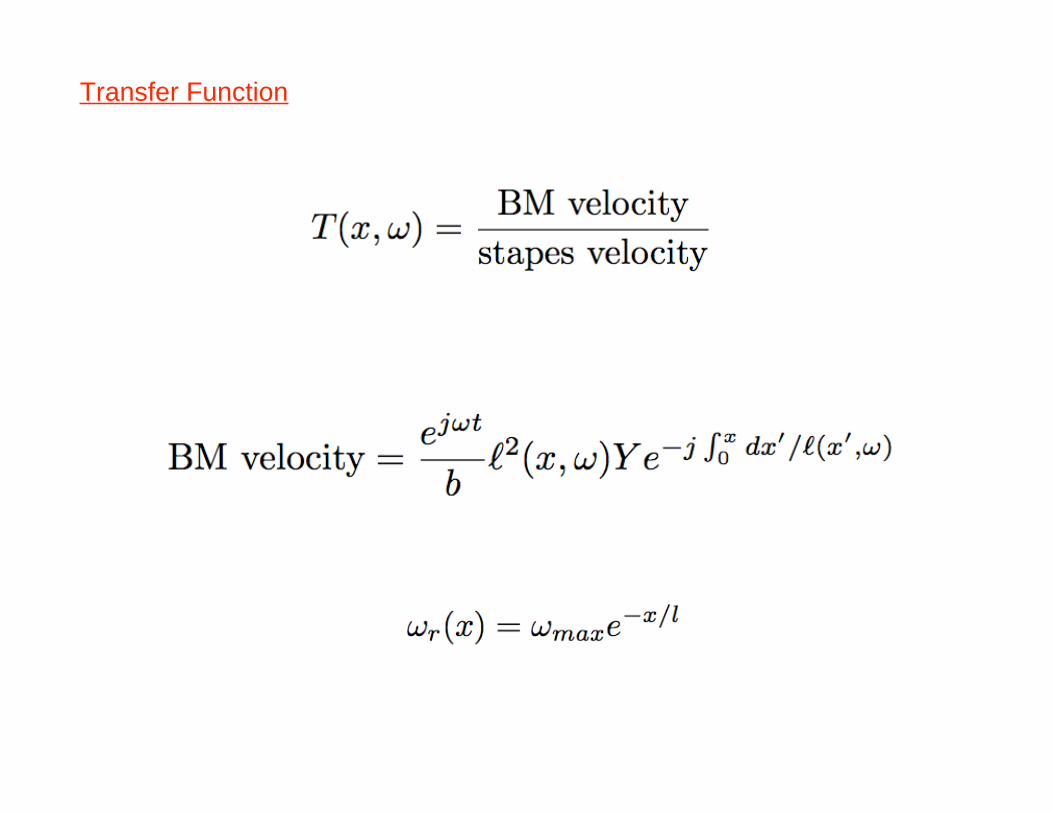
Transfer Function

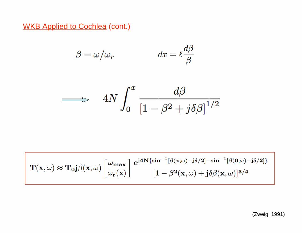
WKB Applied to Cochlea (cont.)

(Zweig, 1991)

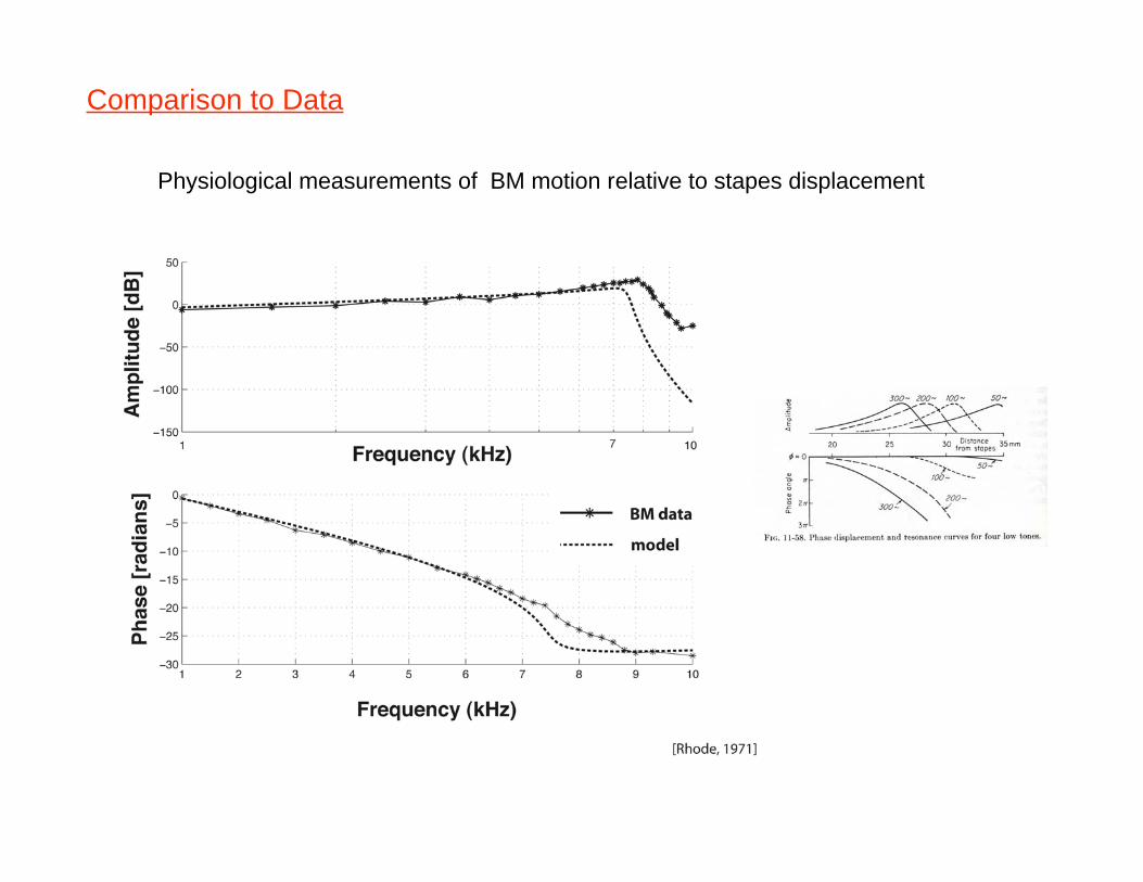
Comparison to Data

Physiological measurements of BM motion relative to stapes displacement

Model provides a starting point for thinking

about cochlear dynamics

What features are present in a real ear

that we would like the model to capture?

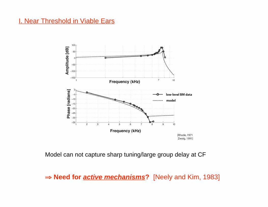
I. Near Threshold in Viable Ears

Model can not capture sharp tuning/large group delay at CF

Need for active mechanisms? [Neely and Kim, 1983]

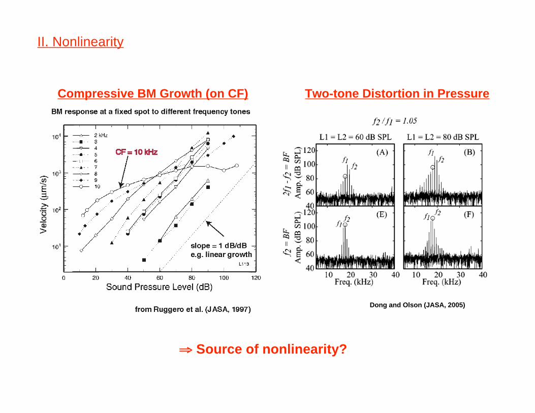
Compressive BM Growth (on CF)

Dong and Olson (JASA, 2005)

Two-tone Distortion in Pressure

II. Nonlinearity

Source of nonlinearity?

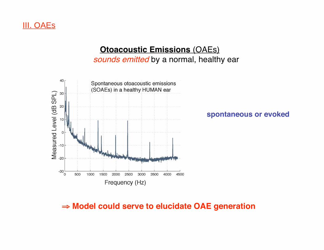
III. OAEs

Otoacoustic Emissions (OAEs) sounds emitted by a normal, healthy ear

spontaneous or evoked

Model could serve to elucidate OAE generation

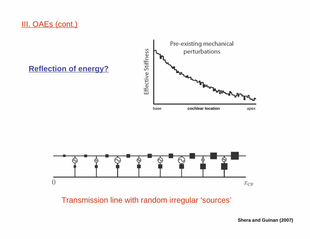
Transmission line with random irregular ‘sources’

Reflection of energy?

Shera and Guinan (2007)

base cochlear location apex

III. OAEs (cont.)

Summary

Developed a passive, linear 1-D transmission line model for

the cochlea

Simple model captures essential features of the cochlea and

can serve as a foundation for more realistic iterations

Ultimate goal is to use cochlear models to better understand

auditory function/physiology and potential clinical applications

Experiments in Hearing (1960)

Georg von Bekesy (1899-1972)