Modeling Chemically Homogeneous Evolution in

COMPAS

Kaila NathanielDepartment of Physics

Virginia Polytechnic Institute and State University

Advisor: Ilya MandelMentors: Coenraad Neijssel, Alejandro Vigna-Gomez

School of Physics and AstronomyUniversity of Birmingham

July 2017

Contents

1 Introduction 2

2 Chemically homogeneous evolution 3

3 Modeling CHE 53.1 Identifying CHE . . . . . . . . . . . . . . . . . . . . . . . . . . . 6

4 Methods 74.1 Convergence Tests . . . . . . . . . . . . . . . . . . . . . . . . . . 74.2 MESA Grids . . . . . . . . . . . . . . . . . . . . . . . . . . . . . 8

5 Results 9

6 Future Work 12

List of Figures

1 Comparison of normal star and a CHE star, with luminosity-temperature lines in the Hertzsprung-Russell diagrams. . . . . . 4

2 Window for CHE in binary stars, with a fixed period of 1.5 days. 63 The purple and teal lines are non-chemically homogeneous stars

evolving normally. The blue, green, and red lines are stars rotat-ing fast enough that they are evolving chemically homogeneously. 7

4 An HR diagram of a 20Msun star, run at the default timestepand 2x the default timestep. The evolution is identical. . . . . . 8

5 ω of normal and chemically homogeneous stars, plotted againstthe Equation 1 line. . . . . . . . . . . . . . . . . . . . . . . . . . 9

6 Comparison of the Equation 1 fit in red and the Equation 6 fitin green. . . . . . . . . . . . . . . . . . . . . . . . . . . . . . . . . 10

7 Plane of data generated for stars with varying mass, ω, and metal-licity. . . . . . . . . . . . . . . . . . . . . . . . . . . . . . . . . . . 11

1

1 Introduction

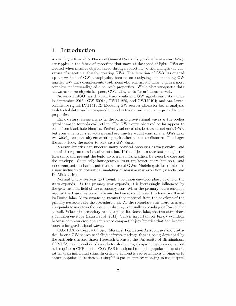
According to Einstein’s Theory of General Relativity, gravitational waves (GW),are ripples in the fabric of spacetime that move at the speed of light. GWs arecreated when massive objects move through spacetime, which changes the cur-vature of spacetime, thereby creating GWs. The detection of GWs has openedup a new field of GW astrophysics, focused on analyzing and modeling GWsignals. GW data complements traditional electromagnetic data to gain a morecomplete understanding of a source’s properties. While electromagnetic dataallows us to see objects in space, GWs allow us to ”hear” them as well.

Advanced LIGO has detected three confirmed GW signals since its launchin September 2015: GW150914, GW151226, and GW170104; and one lower-confidence signal, LVT151012. Modeling GW sources allows for better analysis,as detected data can be compared to models to determine source type and sourceproperties.

Binary stars release energy in the form of gravitational waves as the bodiesspiral inwards towards each other. The GW events observed so far appear tocome from black hole binaries. Perfectly spherical single stars do not emit GWs,but even a neutron star with a small asymmetry would emit smaller GWs thantwo 30M� compact objects orbiting each other at a close distance. The largerthe amplitude, the easier to pick up a GW signal.

Massive binaries can undergo many physical processes as they evolve, andone of those processes is stellar rotation. If the objects rotate fast enough, thelayers mix and prevent the build up of a chemical gradient between the core andthe envelope. Chemically homogeneous stars are hotter, more luminous, andmore compact, and are a potential source of GWs. Modeling stellar rotation isa new inclusion in theoretical modeling of massive star evolution (Mandel andDe Mink 2016).

Normal binary systems go through a common-envelope phase as one of thestars expands. As the primary star expands, it is increasingly influenced bythe gravitational field of the secondary star. When the primary star’s envelopereaches the Lagrange point between the two stars, it is said to have overflowedits Roche lobe. More expansion means that material from the envelope of theprimary accretes onto the secondary star. As the secondary star accretes mass,it expands to maintain thermal equilibrium, eventually expanding its Roche lobeas well. When the secondary has also filled its Roche lobe, the two stars sharea common envelope (Izzard et al. 2011). This is important for binary evolutionbecause common envelope can create compact object binaries that can becomesources for gravitational waves.

COMPAS, or Compact Object Mergers: Population Astrophysics and Statis-tics, is one GW source modeling software package that is being developed bythe Astrophysics and Space Research group at the University of Birmingham.COMPAS has a number of models for developing compact object mergers, butstill requires a CHE model. COMPAS is designed to model populations of stars,rather than individual stars. In order to efficiently evolve millions of binaries toobtain population statistics, it simplifies parameters by choosing to use outputs

2

from prescriptions, in order to evolve stars faster.MESA, or Modules for Experiments in Stellar Astrophysics, is software pri-

marily developed by Bill Paxton of University of California, Santa Barbara,with rotational CHE models mainly written by Pablo Marchant of Argelander-Institut fur Astronomie, Universitat Bonn. MESA can model individual stars inmuch greater detail than COMPAS. In order to develop a detailed CHE modelfor COMPAS, MESA must be used to create more comprehensive prescriptions.While MESA can be used to learn about individual stars in great detail, it isdifficult to determine trends when looking at just a handful of stars at a time.Likewise, COMPAS can determine trends, but is not useful for learning abouthow individual stars behave in great detail. Together, MESA and COMPAScan be used to create detailed prescriptions from individual stars that can thenbe used to evolve millions of binaries to determine overall population trends.

This paper explains the process and methods behind creating prescriptionsfor chemically homogeneous stars using MESA and COMPAS. The rest of thispaper is organized as follows: Section 2 will focus on CHE and its conditions,Section 3 will discuss modeling CHE, Section 4 will explain the methods used,Section 5 will analyze the results from the simulations, and Section 6 will talkabout future possibilities with the work.

2 Chemically homogeneous evolution

The evolution of massive stars, defined here as stars greater than 5M�, can beaffected by multiple physical parameters, such as mass, metallicity and rotation.If a star rotates fast enough, it can trigger mixing between the various layersof chemicals. The mixing changes the chemical composition, or the metallicity,of the star, which affects mass loss from stellar winds and alters the star’sevolution. As might be expected, chemically homogeneous stars evolve verydifferently from their normal counterparts.

The rotation of the star causes the loss of a chemical gradient between thecore and the envelope. The entire star is the core, with no envelope. The mixingmoves material from the hydrogen rich envelope into the central burning regionsand vice versa, creating a star that is approximately chemically homogeneous.While normally evolving stars contract and expand in cycles over time, chemi-cally homogeneous stars only slowly contract as they become more helium rich(Mandel and De Mink 2016). This is because chemically homogeneous starshave no envelope, unlike normal stars.

In most stars, the envelope expands as the core contracts, in order to re-main in hydrostatic equilibrium. However, in very well mixed stars, there is nodistinction between the core and the envelope, and the whole star contracts.This leads to a star that is smaller, hotter, and more luminous than normallyevolved stars (Mandel and De Mink 2016). However, these stars are likely onlyfound in metal-poor environments, because CHE is likely to only be possiblewith metallicity at solar or lower (Martins et al. 2013; Szecsi et al. 2015). AtZ < Z� = 0.02, excessive mass loss due to stellar winds can be avoided. Oth-

3

erwise, the star does not stay well mixed during core hydrogen exhaustion, andis not chemically homogeneous (Marchant et al. 2016).

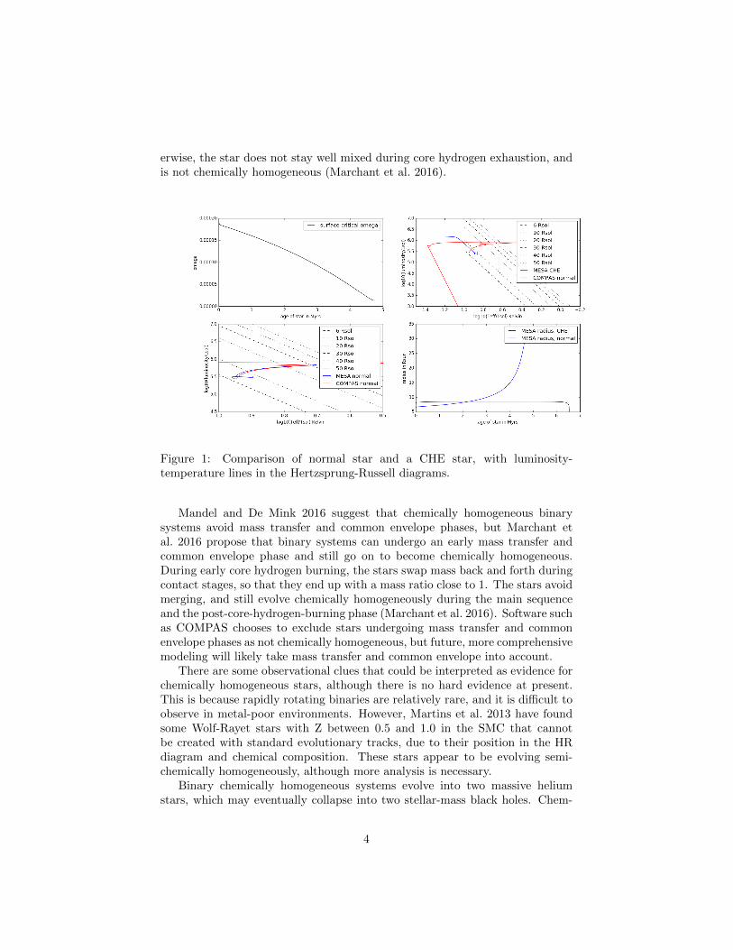
Figure 1: Comparison of normal star and a CHE star, with luminosity-temperature lines in the Hertzsprung-Russell diagrams.

Mandel and De Mink 2016 suggest that chemically homogeneous binarysystems avoid mass transfer and common envelope phases, but Marchant etal. 2016 propose that binary systems can undergo an early mass transfer andcommon envelope phase and still go on to become chemically homogeneous.During early core hydrogen burning, the stars swap mass back and forth duringcontact stages, so that they end up with a mass ratio close to 1. The stars avoidmerging, and still evolve chemically homogeneously during the main sequenceand the post-core-hydrogen-burning phase (Marchant et al. 2016). Software suchas COMPAS chooses to exclude stars undergoing mass transfer and commonenvelope phases as not chemically homogeneous, but future, more comprehensivemodeling will likely take mass transfer and common envelope into account.

There are some observational clues that could be interpreted as evidence forchemically homogeneous stars, although there is no hard evidence at present.This is because rapidly rotating binaries are relatively rare, and it is difficult toobserve in metal-poor environments. However, Martins et al. 2013 have foundsome Wolf-Rayet stars with Z between 0.5 and 1.0 in the SMC that cannotbe created with standard evolutionary tracks, due to their position in the HRdiagram and chemical composition. These stars appear to be evolving semi-chemically homogeneously, although more analysis is necessary.

Binary chemically homogeneous systems evolve into two massive heliumstars, which may eventually collapse into two stellar-mass black holes. Chem-

4

ically homogeneous systems are therefore a potential source of gravitationalwaves. GW observations and analysis may help determine the physics of suchsystems, including their merger rate.

3 Modeling CHE

COMPAS was built upon Hurley, Pols, and Tout 2000; Hurley, Tout, and Pols2002 models, which do not take rotation into account. COMPAS is rapid popu-lation synthesis software, which means that it does not calculate individual starsin detail. Rather than including prescriptions for every parameter, COMPASuses the outputs from the prescriptions when evolving stars. This means thatCOMPAS can evolve large populations, but it requires models, since it cannotcalculate all parameters. COMPAS requires a separate analytical prescriptionto determine which stars, given a mass and metallicity, should be flagged aschemically homogeneous. MESA was used to create that prescription. MESAis stellar evolution code that evolves one star at a time, and evolves them ingreat detail. While MESA does not evolve populations of stars, it can be usedto calculate a prescription that can then be input into population synthesis soft-ware to create large populations. In order to create a prescription for chemicallyhomogeneous stars in COMPAS, it is necessary to model grids of stars undergo-ing CHE in MESA, and then translate the data into a prescription that can becoded into COMPAS. This requires learning how to identify stars undergoingCHE, both manually and automatically; and then how to evolve stars so thatthey undergo CHE. Once the boundaries for CHE are understood, a fit can bemade from the data, and a prescription can be put into COMPAS.

Mandel and De Mink 2016 approximated a basic model with a minimumωc for single stars to evolve quasi-chemically homogeneously using a Z = 0.004grid.

ωc =

{0.2 + 2.7×10−4( m

M�− 50)2 for m < 50M�

0.2 for m ≥ 50M�(1)

Using Kepler’s Third Law, a threshold period can be found for binary starsundergoing CHE. Once a threshold period is found, it is easy to calculate the ωof a star to see if it is greater than the ωc, and therefore undergoing CHE.

P =πr

32

√GM

(2)

ω =2πr

Pvk≥ ωc (3)

vk =

√Gm

r(4)

Where vk is the Keplerian velocity, M is the combined masses of the binarysystem, and m is the mass of a single star. r can be taken as the star radius, orcan be approximated with the following formula at solar metallicity.

5

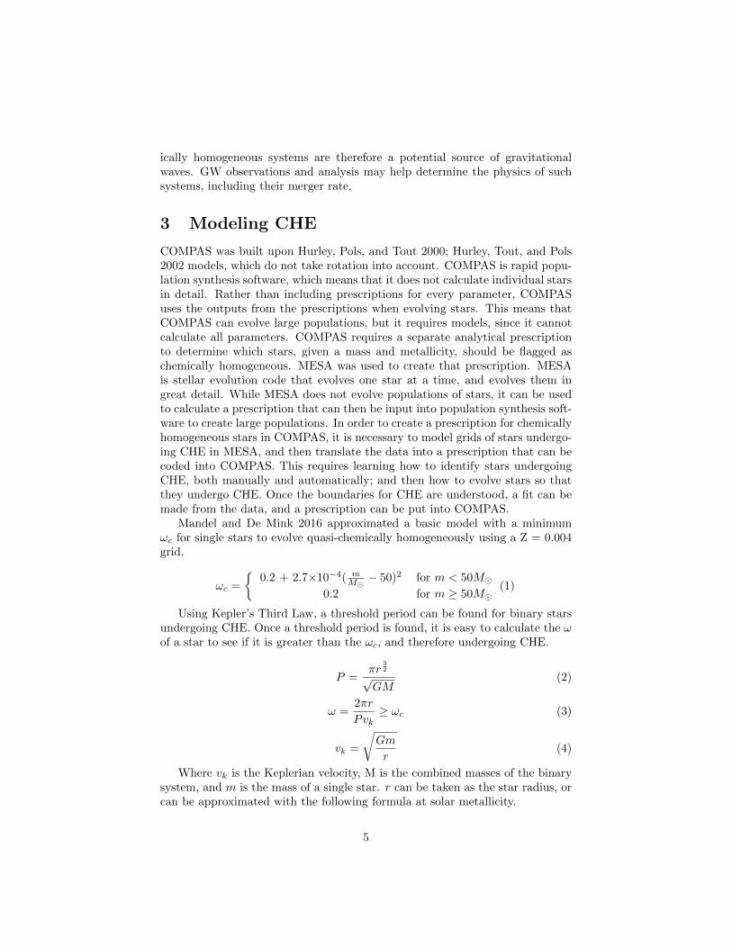
r = R�( MM�

)0.6 for m > M� (5)

At low metallicities, this radius formula is no longer very accurate. Calcula-tions at Z = 0.004 show that the radius is about 1.2 times larger than the trueradius of the star. There is not currently a better fit for the radius, as only arough approximation is necessary.

Figure 2: Window for CHE in binary stars, with a fixed period of 1.5 days.

However, these formulae can only be used to create chemically homogeneousbinaries, rather than single stars, and it is a definition of CHE that does nottake chemical composition into account.

3.1 Identifying CHE

In order to create a prescription for chemically homogeneous stars in COMPAS,it is necessary to model individual stars undergoing CHE in MESA, and thentranslate the data into a prescription that can be coded into COMPAS. Thisrequires learning how to identify stars undergoing CHE, both manually andautomatically; and then how to evolve stars so that they undergo CHE.

While a regular star’s HR diagram goes to the right after ZAMS, a starundergoing CHE has a HR that diverts to the left after ZAMS is completed.Additionally, a regular star has its radius expand as it evolves, while a starundergoing CHE has a radius that stays fairly constant until near the end ofits life, where the radius will rapidly decrease as the star contracts. This is

6

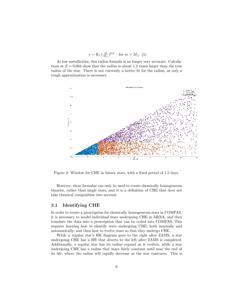
because a CHE star does not have a separate core and envelope, so there is noexpansion and contraction over the lifetime of the star. These are indicators thatcan be seen visually in plots, but are difficult to detect automatically. A betterway to detect stars that are undergoing CHE is by chemical composition in thecore and surface of the star. A normal star will have a fairly large differencebetween the abundance of helium in the surface and the core, while a chemicallyhomogeneous star will have a much smaller difference. As per Marchant et al.2016, stars that reach a point where the difference between the surface and corehelium abundance is greater than 0.2 are deemed to be evolving normally. Starswith a difference of less than or equal to 0.2 are chemically homogeneous andflagged as such.

Figure 3: The purple and teal lines are non-chemically homogeneous stars evolv-ing normally. The blue, green, and red lines are stars rotating fast enough thatthey are evolving chemically homogeneously.

4 Methods

4.1 Convergence Tests

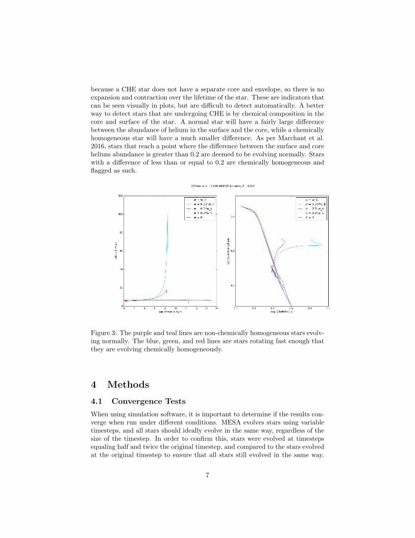
When using simulation software, it is important to determine if the results con-verge when run under different conditions. MESA evolves stars using variabletimesteps, and all stars should ideally evolve in the same way, regardless of thesize of the timestep. In order to confirm this, stars were evolved at timestepsequaling half and twice the original timestep, and compared to the stars evolvedat the original timestep to ensure that all stars still evolved in the same way.

7

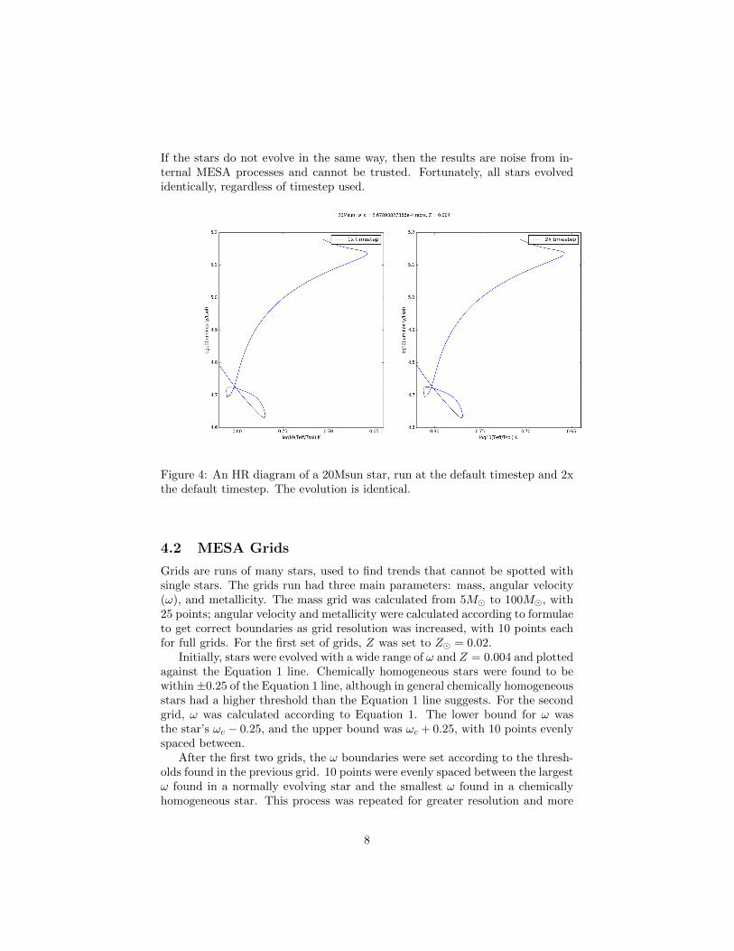
If the stars do not evolve in the same way, then the results are noise from in-ternal MESA processes and cannot be trusted. Fortunately, all stars evolvedidentically, regardless of timestep used.

Figure 4: An HR diagram of a 20Msun star, run at the default timestep and 2xthe default timestep. The evolution is identical.

4.2 MESA Grids

Grids are runs of many stars, used to find trends that cannot be spotted withsingle stars. The grids run had three main parameters: mass, angular velocity(ω), and metallicity. The mass grid was calculated from 5M� to 100M�, with25 points; angular velocity and metallicity were calculated according to formulaeto get correct boundaries as grid resolution was increased, with 10 points eachfor full grids. For the first set of grids, Z was set to Z� = 0.02.

Initially, stars were evolved with a wide range of ω and Z = 0.004 and plottedagainst the Equation 1 line. Chemically homogeneous stars were found to bewithin±0.25 of the Equation 1 line, although in general chemically homogeneousstars had a higher threshold than the Equation 1 line suggests. For the secondgrid, ω was calculated according to Equation 1. The lower bound for ω wasthe star’s ωc − 0.25, and the upper bound was ωc + 0.25, with 10 points evenlyspaced between.

After the first two grids, the ω boundaries were set according to the thresh-olds found in the previous grid. 10 points were evenly spaced between the largestω found in a normally evolving star and the smallest ω found in a chemicallyhomogeneous star. This process was repeated for greater resolution and more

8

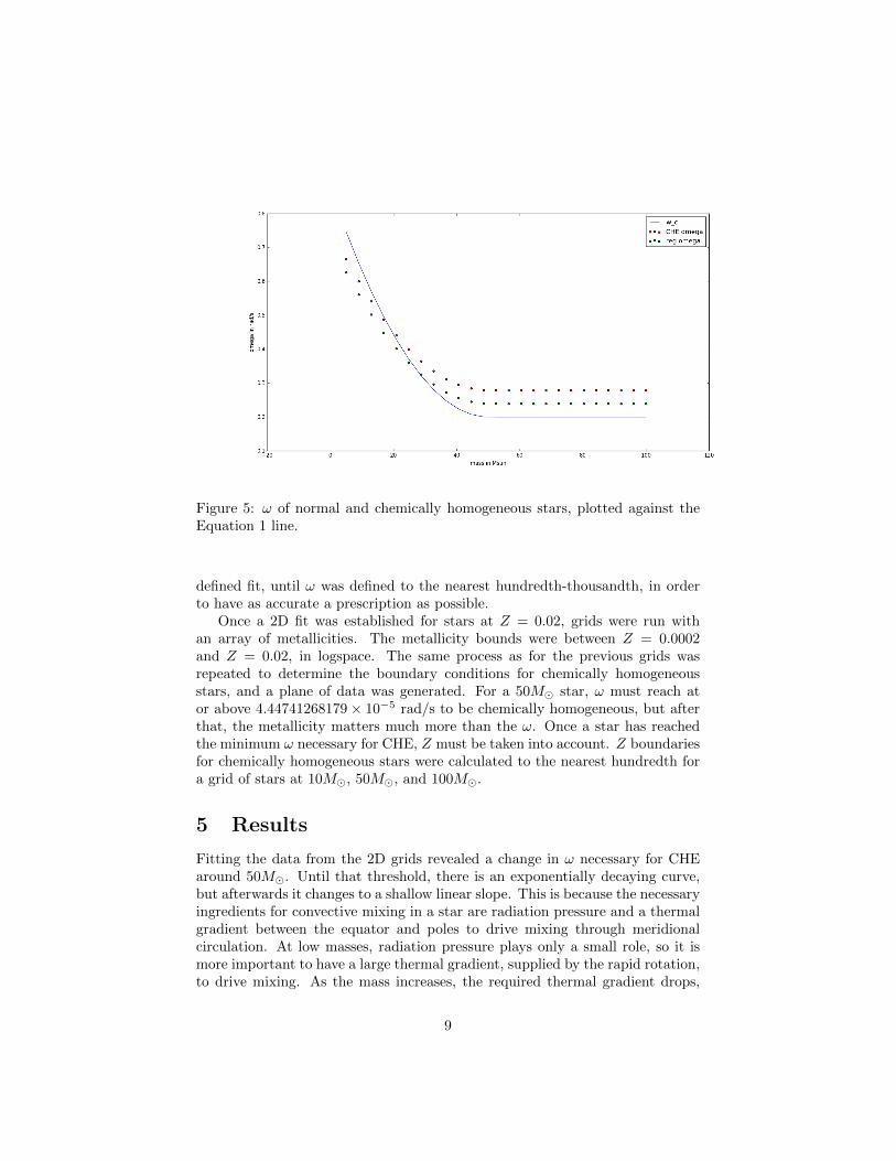
Figure 5: ω of normal and chemically homogeneous stars, plotted against theEquation 1 line.

defined fit, until ω was defined to the nearest hundredth-thousandth, in orderto have as accurate a prescription as possible.

Once a 2D fit was established for stars at Z = 0.02, grids were run withan array of metallicities. The metallicity bounds were between Z = 0.0002and Z = 0.02, in logspace. The same process as for the previous grids wasrepeated to determine the boundary conditions for chemically homogeneousstars, and a plane of data was generated. For a 50M� star, ω must reach ator above 4.44741268179× 10−5 rad/s to be chemically homogeneous, but afterthat, the metallicity matters much more than the ω. Once a star has reachedthe minimum ω necessary for CHE, Z must be taken into account. Z boundariesfor chemically homogeneous stars were calculated to the nearest hundredth fora grid of stars at 10M�, 50M�, and 100M�.

5 Results

Fitting the data from the 2D grids revealed a change in ω necessary for CHEaround 50M�. Until that threshold, there is an exponentially decaying curve,but afterwards it changes to a shallow linear slope. This is because the necessaryingredients for convective mixing in a star are radiation pressure and a thermalgradient between the equator and poles to drive mixing through meridionalcirculation. At low masses, radiation pressure plays only a small role, so it ismore important to have a large thermal gradient, supplied by the rapid rotation,to drive mixing. As the mass increases, the required thermal gradient drops,

9

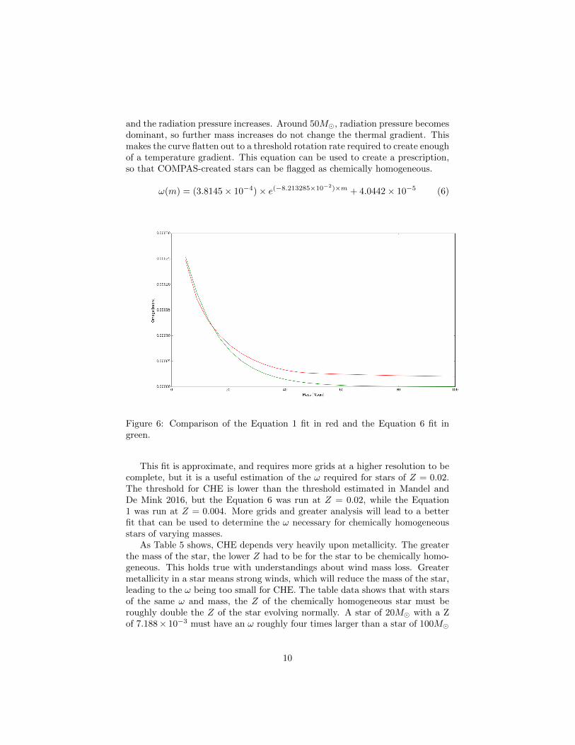
and the radiation pressure increases. Around 50M�, radiation pressure becomesdominant, so further mass increases do not change the thermal gradient. Thismakes the curve flatten out to a threshold rotation rate required to create enoughof a temperature gradient. This equation can be used to create a prescription,so that COMPAS-created stars can be flagged as chemically homogeneous.

ω(m) = (3.8145× 10−4)× e(−8.213285×10−2)×m + 4.0442× 10−5 (6)

Figure 6: Comparison of the Equation 1 fit in red and the Equation 6 fit ingreen.

This fit is approximate, and requires more grids at a higher resolution to becomplete, but it is a useful estimation of the ω required for stars of Z = 0.02.The threshold for CHE is lower than the threshold estimated in Mandel andDe Mink 2016, but the Equation 6 was run at Z = 0.02, while the Equation1 was run at Z = 0.004. More grids and greater analysis will lead to a betterfit that can be used to determine the ω necessary for chemically homogeneousstars of varying masses.

As Table 5 shows, CHE depends very heavily upon metallicity. The greaterthe mass of the star, the lower Z had to be for the star to be chemically homo-geneous. This holds true with understandings about wind mass loss. Greatermetallicity in a star means strong winds, which will reduce the mass of the star,leading to the ω being too small for CHE. The table data shows that with starsof the same ω and mass, the Z of the chemically homogeneous star must beroughly double the Z of the star evolving normally. A star of 20M� with a Zof 7.188× 10−3 must have an ω roughly four times larger than a star of 100M�

10

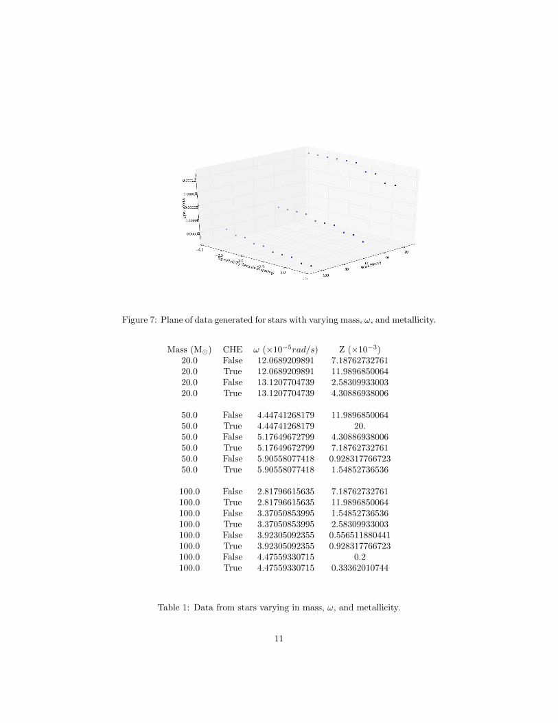
Figure 7: Plane of data generated for stars with varying mass, ω, and metallicity.

Mass (M�) CHE ω (×10−5rad/s) Z (×10−3)20.0 False 12.0689209891 7.1876273276120.0 True 12.0689209891 11.989685006420.0 False 13.1207704739 2.5830993300320.0 True 13.1207704739 4.30886938006

50.0 False 4.44741268179 11.989685006450.0 True 4.44741268179 20.50.0 False 5.17649672799 4.3088693800650.0 True 5.17649672799 7.1876273276150.0 False 5.90558077418 0.92831776672350.0 True 5.90558077418 1.54852736536

100.0 False 2.81796615635 7.18762732761100.0 True 2.81796615635 11.9896850064100.0 False 3.37050853995 1.54852736536100.0 True 3.37050853995 2.58309933003100.0 False 3.92305092355 0.556511880441100.0 True 3.92305092355 0.928317766723100.0 False 4.47559330715 0.2100.0 True 4.47559330715 0.33362010744

Table 1: Data from stars varying in mass, ω, and metallicity.

11

with the same Z. There is not currently a fit equation for Table 5, but theanalysis is in process.

6 Future Work

The overall goal of this project was to create an equation that would determinethe ω necessary to create chemically homogeneous stars of varying masses andmetallicities that can then be input into a model for CHE in COMPAS. Anequation has been found for stars of varying masses, and the next step is tocreate a COMPAS model. To do this, a new stellar evolution type must becreated in COMPAS. While Marchant et al. 2016 determined that stars canundergo early mass transfer and still go on to be chemically homogeneous, fornow the COMPAS model will assume that stars undergoing mass transfer arenot eligible to become chemically homogeneous. Normal wind prescriptions willstill apply, and the star will basically turn into a zero-age Wolf-Rayet star,evolving as a Hurley HeMS once it reaches HeMS. It will be assumed that thewhole star becomes a helium core, with existing COMPAS prescriptions takingover once the star reaches HeMS.

Another future goal is to create an equation that can be used to determinechemically homogeneous stars of varying masses and metallicities. Currentlyexisting equations are for stars at Z = 0.004 and Z = 0.02, and it would behelpful to have a prescription that can be used at an arbitrary metallicity. Thisrequires more grids with greater resolution, and more analysis of results. Thiswork is currently ongoing.

12

References

Hurley, Jarrod R., O. R. Pols, and Christopher A. Tout (2000). “Comprehensiveanalytic formulae for stellar evolution as a function of mass and metallicity”.In: Royal Astronomical Society 315, pp. 543–569.

Hurley, Jarrod R., Christopher A. Tout, and O. R. Pols (2002). “Evolutionof binary stars and the effect of tides on binary populations”. In: RoyalAstronomical Society 329.4, pp. 897–928.

Izzard, Robert G. et al. (2011). “Common envelope evolution”. In: IAU Sympo-sium.

Mandel, I. and S. E. De Mink (2016). “Merging Binary Black Holes FormedThrough Chemically Homogeneous Evolution in Short-Period Stellar Bina-ries”. In: MSRAS.

Marchant, Pablo et al. (2016). “A new route towards merging massive blackholes”. In: Astronomy and Astrophysics.

Martins, F. et al. (2013). “Evidence for quasi-chemically homogeneous evolutionof massive stars up to solar metallicity”. In: Astronomy and Astrophysics.

Szecsi, Dorottya et al. (2015). “Low-metallicity massive single stars with rota-tion”. In: Astronomy and Astrophysics.

13