Modeling blue and green water availability ... - swat.tamu.edu · analysis techniques in connection to SWAT and found that SUFI-2 needed the smallest number of model runs to achieve

Modeling blue and green water availability in Africa

Jurgen Schuol,1,2 Karim C. Abbaspour,1 Hong Yang,1 Raghavan Srinivasan,3

and Alexander J. B. Zehnder4

Received 23 October 2007; revised 30 January 2008; accepted 14 February 2008; published 9 July 2008.

[1] Despite the general awareness that in Africa many people and large areas are sufferingfrom insufficient water supply, spatially and temporally detailed information onfreshwater availability and water scarcity is so far rather limited. By applyinga semidistributed hydrological model SWAT (Soil and Water Assessment Tool), thefreshwater components blue water flow (i.e., water yield plus deep aquifer recharge),green water flow (i.e., actual evapotranspiration), and green water storage (i.e., soil water)were estimated at a subbasin level with monthly resolution for the whole of Africa. Usingthe program SUFI-2 (Sequential Uncertainty Fitting Algorithm), the model wascalibrated and validated at 207 discharge stations, and prediction uncertainties werequantified. The presented model and its results could be used in various advanced studieson climate change, water and food security, and virtual water trade, among others.The model results are generally good albeit with large prediction uncertainties in somecases. These uncertainties, however, disclose the actual knowledge about the modeledprocesses. The effect of considering these model-based uncertainties in advancedstudies is shown for the computation of water scarcity indicators.

Citation: Schuol, J., K. C. Abbaspour, H. Yang, R. Srinivasan, and A. J. B. Zehnder (2008), Modeling blue and green water

availability in Africa, Water Resour. Res., 44, W07406, doi:10.1029/2007WR006609.

1. Introduction

[2] On a continental and annual basis Africa has abun-dant water resources but the problem is their high spatialand temporal variability within and between countries andriver basins [UN-Water/Africa, 2006]. Considering thisvariability, the continent can be seen as dry with pressingwater problems [Falkenmark, 1989; Vorosmarty et al.,2005]. Though of critical importance, detailed informationon water resources and water scarcity is still limited inAfrica [Wallace and Gregory, 2002].[3] Freshwater availability is a prerequisite for food secu-

rity, public health, ecosystem protection, etc. Thus freshwateris important and relevant for achieving all development goalscontained in the United Nations Millennium Declaration(http://www.un.org/millennium/declaration/ares552e.pdf).Two important targets of the Declaration are to halve, by theyear 2015, the proportion of people without sustainableaccess to safe drinking water and to halve the proportion ofpeople who suffer from hunger. These two targets are closelyrelated to freshwater availability.

[4] Up to now, studies of freshwater availability havepredominantly focused on the quantification of the ‘‘bluewater’’, while ignoring the ‘‘green water’’ as part of thewater resource and its great importance especially forrainfed agriculture (e.g., in sub-Saharan Africa more than95% is rainfed [Rockstrom et al., 2007]). Two of the fewstudies dealing with green water are Rockstrom and Gordon[2001] and Gerten et al. [2005]. Blue water flow, or theinternal renewable water resource (IRWR), is traditionallyquantified as the sum of the water yield and the deep aquiferrecharge. Green water, on the other hand, originates fromthe naturally infiltrated water, which is more and more beingthought of as a manageable water resource. Falkenmarkand Rockstrom [2006] differentiate between two compo-nents of the green water: green water resource (or storage),which equals the moisture in the soil, and green water flow,which equals the sum of the actual evaporation (thenonproductive part) and the actual transpiration (the pro-ductive part). In some references only the transpiration isregarded as the green water component [e.g., Savenije,2004]. As evaporation and transpiration are closely inter-linked processes and evaporated water has the potential tobe partly used as productive flow for food production, weprefer to consider the total actual evapotranspiration as thegreen water flow.[5] Spatially and temporally detailed assessments of the

different components of freshwater availability are essentialfor locating critical regions, and thus, the basis for rationaldecision-making in water resources planning and manage-ment. There exist already a few global freshwater assess-ments based on (1) data generalization [e.g., Shiklomanov,2000; Shiklomanov and Rodda, 2003], (2) general circula-tion models (GCMs), [e.g., TRIP, Oki et al., 2001; Oki and

1Department System Analysis, Integrated Assessment and Modelling,

Eawag, Swiss Federal Institute of Aquatic Science and Technology,Dubendorf, Switzerland.

2Swiss Federal Institute of Technology, Zurich, Switzerland.3Spatial Sciences Laboratory, Texas A&M University, Texas Agricultural

Experimental Station, College Station, Texas, USA.4Board of the Swiss Federal Institutes of Technology, ETH-Zentrum,

Zurich, Switzerland.

Copyright 2008 by the American Geophysical Union.0043-1397/08/2007WR006609$09.00

W07406

WATER RESOURCES RESEARCH, VOL. 44, W07406, doi:10.1029/2007WR006609, 2008ClickHere

for

FullArticle

1 of 18

http://dx.doi.org/10.1029/2007WR006609

Kanae, 2006], and (3) hydrological models [e.g., WBM,Vorosmarty et al., 1998, 2000; Fekete et al., 1999; Macro-PDM, Arnell, 1999; WGHM (WaterGAP 2), Alcamo et al.,2003; Doll et al., 2003; LPJ, Gerten et al., 2004; WAS-MOD-M, Widen-Nilsson et al., 2007]. GCMs with theirstrength on the atmospheric model component performpoorly on the soil water processes [Doll et al., 2003]. Allthe above mentioned hydrological models are raster modelswith a spatial resolution of 0.5� but show different degreesof complexities. These models either have not been cali-brated (e.g., WBM) or only one (e.g., WGHM) or fewparameters (e.g., WASMOD-M) have been checked andadjusted against long-term average runoffs. In WGHM, forsome basins one or two correction factors have beenadditionally applied in order to guarantee a maximum of1% error of the simulated long-term annual average runoff[Doll et al., 2003]. Intraannual runoff differences, which areof key importance in many regions have been included insome studies [e.g., Widen-Nilsson et al., 2007] but not usedfor calibration.[6] The existing global and continental freshwater assess-

ment models have been used for climate and socio-eco-nomic change scenarios [Alcamo et al., 2007], water stresscomputation [Vorosmarty et al., 2005], analysis of seasonaland interannual continental water storage variations [Guntneret al., 2007], global water scarcity analysis taking intoaccount environmental water requirements [Smakhtin et al.,2004], and virtual water trading [Islam et al., 2007] amongothers. Hence it is important that these models pass through acareful calibration, validation, and uncertainty analysis.Particularly in large-scale (hydrological) models, theexpected uncertainties are rather large. For this task, severaldifferent procedures have been developed: e.g., GeneralizedLikelihood Uncertainty Estimation (GLUE) [Beven andBinley, 1992], Bayesian inference based on Markov ChainMonte Carlo (MCMC) [Vrugt et al., 2003], ParameterSolution (ParaSol) [van Griensven and Meixner, 2006],and Sequential Uncertainty Fitting (SUFI-2) [Abbaspouret al., 2007].[7] In this study, we modeled the monthly subcountry-

based freshwater availability for Africa and explicitly dif-ferentiated between the different freshwater components:blue water flow, green water storage and green water flow.The model of choice was ‘‘Soil and Water AssessmentTool’’ (SWAT) [Arnold et al., 1998] because of two reasons.First, SWAT has been already successfully applied for waterquantity and quality issues for a wide range of scales andenvironmental conditions around the globe. A comprehen-sive SWAT review paper summarizing the findings of morethan 250 peer-reviewed articles is written by Gassman et al.[2007]. The suitability of SWAT for very large scalesapplications has been shown in the ‘‘Hydrologic Unit Modelfor the United States’’ project (HUMUS) [Arnold et al.,1999; Srinivasan et al., 1998]. SWAT was recently alsoapplied in the national and watershed assessments of theU.S. Department of Agriculture (USDA) ConservationEffects Assessment Program (CEAP, http://www.nrcs.usda.gov/Technical/nri/ceap/index.html). The second reason forchoosing SWAT for this exclusive water quantity study wasits ability to perform plant growth and water qualitymodeling, a topic we plan to study in the future. Anadvantage of SWAT is its modular implementation where

processes can be selected or not. As processes are repre-sented by parameters in the model, in data scarce regionsSWAT can run with a minimum number of parameters. Asmore is known about a region, more processes can beinvoked for by updating and running the model again.[8] The African model was calibrated and validated at

207 discharge stations across the continent. Uncertaintieswere quantified using SUFI-2 program [Abbaspour et al.,2007]. Yang et al. [2008] compared different uncertaintyanalysis techniques in connection to SWAT and found thatSUFI-2 needed the smallest number of model runs toachieve a similarly good solution and prediction uncertainty.This efficiency issue is of great importance when dealingwith computationally intensive, complex, and large-scalemodels. In addition, SUFI-2 is linked to SWAT (in theSWAT-CUP software) [Abbaspour et al., 2008] through aninterface that includes also the programs GLUE, ParaSol,and MCMC.

2. Materials and Methods

2.1. SWAT2005 Model and ArcSWAT Interface

[9] To simulate the water resources availability in Africa,the latest version of the semiphysically based, semidistrib-uted, basin-scale model SWAT [Arnold et al., 1998] wasselected (SWAT2005) [Neitsch et al., 2005]. SWAT is acontinuous time model and operates on a daily time step.Only the hydrologic component of the model was used inthis study. In SWAT the modeled area is divided intomultiple subbasins by overlaying elevation, land cover, soil,and slope classes. In this study the subbasins were charac-terized by dominant land-use, soil, and slope classes. Thischoice was essential for keeping the size of the model at apractical limit. For each of the subunits, water balance wassimulated for four storage volumes: snow, soil profile,shallow aquifer, and deep aquifer. In our case, potential evapo-transpiration was computed using the Hargreaves methodwhich requires the climatic input of daily precipitation, andminimum and maximum temperature. Surface runoff wassimulated using a modification of the SCS Curve Number(CN) method. Despite the empirical nature, this approach hasbeen proven to be successful for many applications and a widevariety of hydrologic conditions [Gassman et al., 2007]. Therunoff from each subbasin was routed through the rivernetwork to the main basin outlet using, in our case, thevariable storage method. Further technical model details aregiven by Arnold et al. [1998] and Neitsch et al. [2005].[10] The preprocessing of the SWAT model input (e.g.,

watershed delineation, manipulation of the spatial andtabular data) was performed within ESRI ArcGIS 9.1 usingthe ArcSWAT interface [Winchell et al., 2007]. In compar-ison to the ArcView GIS interface AVSWAT2000 [Di Luzioet al., 2001], ArcSWAT has no apparent limitationconcerning the size and complexity of the simulated areaas it was able to model the entire African continent.

2.2. Calibration and Uncertainty AnalysisProcedure SUFI-2

[11] The program SUFI-2 [Abbaspour et al., 2007] wasused for a combined calibration and uncertainty analysis. Inany (hydrological) modeling work there are uncertainties ininput (e.g., rainfall), in conceptual model (e.g., by process

2 of 18

W07406 SCHUOL ET AL.: MODELING BLUE AND GREEN WATER AVAILABILITY IN AFRICA W07406

simplification or by ignoring important processes), inmodel parameters (nonuniqueness) and in the measureddata (e.g., discharge used for calibration). SUFI-2 mapsthe aggregated uncertainties to the parameters and aims toobtain the smallest parameter uncertainty (ranges). Theparameter uncertainty leads to uncertainty in the outputwhich is quantified by the 95% prediction uncertainty(95PPU) calculated at the 2.5% (L95PPU) and the 97.5%(U95PPU) levels of the cumulative distribution obtainedthrough Latin hypercube sampling. Starting with large butphysically meaningful parameter ranges that bracket ‘most’of the measured data within the 95PPU, SUFI-2 decreasesthe parameter uncertainties iteratively. After each iteration,new and narrower parameter uncertainties are calculated[see Abbaspour et al., 2007] where the more sensitiveparameters find a larger uncertainty reduction than the lesssensitive parameters. In deterministic simulations, output(i.e., river discharge) is a signal and can be compared to ameasured signal using indices such as R2, root mean squareerror, or Nash-Sutcliffe. In stochastic simulations wherepredicted output is given by a prediction uncertainty bandinstead of a signal, we devised two different indices tocompare measurement to simulation: the P-factor and theR-factor [Abbaspour et al., 2007]. These indices wereused to gauge the strength of calibration and uncertaintymeasures. The P-factor is the percentage of measured databracketed by the 95PPU. As all correct processes andmodel inputs are reflected in the observations, the degreeto which they are bracketed in the 95PPU indicates thedegree to which the model uncertainties are beingaccounted for. The maximum value for the P-factor is100%, and ideally we would like to bracket all measureddata, except the outliers, in the 95PPU band. The R-factoris calculated as the ratio between the average thickness ofthe 95PPU band and the standard deviation of the measureddata. It represents the width of the uncertainty interval andshould be as small as possible. R-factor indicates thestrength of the calibration and should be close to or smallerthan a practical value of 1. As a larger P-factor can befound at the expense of a larger R-factor, often a trade offbetween the two must be sought.

2.3. Database

[12] The model for the continent of Africa was con-structed using in most cases freely available global infor-mation. The collection of the data was followed by anaccurate compilation and analysis of the quality and integrity.The basic input maps included the digital elevation model(DEM) GTOPO30, the digital stream network HYDRO1k(http://edc.usgs.gov/products/elevation/gtopo30/hydro/index.html), and the land cover map Global Land CoverCharacterization (GLCC) (http://edcsns17.cr.usgs.gov/glcc/)both at a resolution of 1 km from U.S. Geological Survey(USGS). The soil map was produced by the Food andAgriculture Organization of the United Nations [FAO,1995] at a resolution of 10 km, including almost 5000 soiltypes and two soil layers. Because of the few and unevenlydistributed weather stations in Africa with often only shortand erroneous time series, the daily weather input (precipi-tation, minimum and maximum temperature) was generatedfor each subbasin based on the 0.5� grids monthly statisticsfrom Climatic Research Unit (CRU TS 1.0 and 2.0, http://www.cru.uea.ac.uk/cru/data/hrg.htm). We developed a semi-

automated weather generator, dGen, for this purpose [Schuoland Abbaspour, 2007]. Information on lakes, wetlands andreservoirs was extracted from the Global Lakes andWetlandsDatabase (GLWD) [Lehner and Doll, 2004]. River dischargedata, which is essential for calibration and validation, wereobtained from the Global Runoff Data Centre (GRDC, http://grdc.bafg.de). More details on the databases are discussed bySchuol et al. [2008].

2.4. Model Setup

[13] The ArcSWAT interface was used for the setup andparameterization of the model. On the basis of the DEM andthe stream network, a minimum drainage area of 10,000 km2

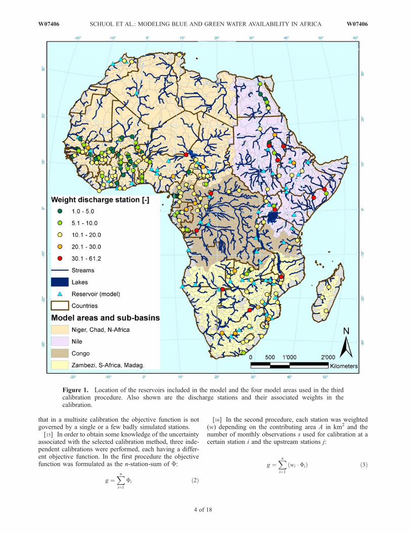
was chosen to discretize the continent into 1496 subbasins.The geomorphology, stream parameterization, and overlayof soil and land cover were automatically done within theinterface. To mitigate the effect of land cover change overtime, and to decrease the computational time of the verylarge-scale model, the dominant soil and land cover wereused in each subbasin. The simulation period was from1968 to 1995 and for these years we provided dailygenerated weather input. The first 3 years were used aswarm-up period to mitigate the unknown initial conditionsand were excluded from the analysis. Lakes, wetlands, andreservoirs, which affect the river discharge to a great extent,were also included in the model. As detail information waslacking, only 64 reservoirs with storage volumes larger than1 km3 were included (Figure 1). In this study, wetlands onthe main channel networks as well as lakes were treated asreservoirs. The parameterization was mostly based oninformation from GLWD-1 [Lehner and Doll, 2004].

2.5. Model Calibration Procedures

[14] Model calibration and validation is a necessary,challenging but also to a certain degree subjective step inthe development of any complex hydrological model. TheAfrican model was calibrated using monthly river dis-charges from 207 stations. These stations were unevenlydistributed throughout the continent (Figure 1) and covered,in most cases, only parts of the whole analysis period from1971 to 1995. For this reason it was inevitable to includedifferent time lengths (minimum of 3 years) and timeperiods at the different stations in the calibration procedure.Consistently at all stations, using a split-sample procedure,the more recent half of the discharge data were used forcalibration and the prior half were used for validation. Inorder to compare the monthly measured and simulateddischarges, F, a weighted version of the coefficient ofdetermination (slightly modified [Krause et al., 2005])was selected as efficiency criteria:

F ¼jbjR2 if jbj � 1

jbj�1R2 if jbj > 1

8<: ð1Þ

where the coefficient of determination R2 represents thedischarge dynamics, and b is the slope of the regression linebetween the monthly observed and simulated runoff.Including b guarantees that runoff under- or over-predic-tions are also reflected. A major advantage of this efficiencycriterion is that it ranges from 0 to 1, which compared toNash-Sutcliff coefficient with a range of �1 to 1, ensures

W07406 SCHUOL ET AL.: MODELING BLUE AND GREEN WATER AVAILABILITY IN AFRICA

3 of 18

W07406

that in a multisite calibration the objective function is notgoverned by a single or a few badly simulated stations.[15] In order to obtain some knowledge of the uncertainty

associated with the selected calibration method, three inde-pendent calibrations were performed, each having a differ-ent objective function. In the first procedure the objectivefunction was formulated as the n-station-sum of F:

g ¼Xni¼1

Fi ð2Þ

[16] In the second procedure, each station was weighted(w) depending on the contributing area A in km2 and thenumber of monthly observations s used for calibration at acertain station i and the upstream stations j:

g ¼Xni¼1

wi � Fið Þ ð3Þ

Figure 1. Location of the reservoirs included in the model and the four model areas used in the thirdcalibration procedure. Also shown are the discharge stations and their associated weights in thecalibration.

4 of 18


where

wi ¼

ffiffiffiffiffiffiffiffiffiffiffiffiffiffiffiffiffiffiffiffiffiffiffiffiffiffiffiffiffiffiffiffiffiffiAi �

Pnj¼1

Aj

!� si

si þPnj¼1

sj

vuuuuuuut ð4Þ

[17] The idea behind this weighting is that a runoff stationwith a long data series and a large watershed without furtherstations upstream provides more information for calibrationand should have a larger weight than a station in a denselygauged area or a station with a short time series. Theweights ranged from 1 to 61 for the furthest downstreamstation on the river Congo at Kinshasa (Figure 1).[18] In the third calibration procedure the region was

divided into four modeling zones and each zone wascalibrated independently. The four model areas basicallydelineated the large river basins in the continent (Figure 1)and included: Area 1, Niger, Chad, and North Africa withan area of 11.8 million km2 and 106 stations; Area 2, Nilewith an area of 6.1 million km2 and 27 stations; Area 3,Congo with an area of 4.8 million km2 and 38 stations; andArea 4, Zambezi, South Africa, and Madagascar with anarea of 5.1 million km2 and 36 stations. The zoning wasbased on the intracontinental variations in the climate aswell as the dominant land covers and soil types.[19] The choice of the parameters initially included in the

calibration procedures was based on the experience gainedin modeling West Africa [Schuol et al., 2008] for which adetailed literature-based preselection as well as a sensitivityanalysis has been performed. Some of the selected SWATparameters (e.g., curve number) are closely related to landcover, while some others (e.g., available water capacity,bulk density) are related to soil texture. For these parametersa separate value for each land-cover/soil-texture was

selected, which increased the number of calibrated param-eters substantially. The percentage of land cover and soiltexture distribution within Africa and the four subregions islisted in Table 1. In the course of the iterative SUFI-2calibration, not only the parameter ranges were narrowed,but also the number of parameters was decreased byexcluding those that turned out to be insensitive.[20] To account for the uncertainty in the measured dis-

charge data, a relative error of 10% [Butts et al., 2004] andan absolute measured discharge uncertainty of 0.1 m3 s�1

were included when calculating the P-factor. The absoluteuncertainty was included in order to capture the dry periodsof the many intermittent streams.

3. Results and Analysis

3.1. Model Calibration

[21] The three calibration procedures produced more orless similar results for the whole of Africa in terms of thevalues of the objective function F, the P-factor, and theR-factor (Table 2). The final parameter ranges in the threeprocedures, although different, were clustered around thesame regions of the parameter space as shown in Table 3.This is typical of a nonuniqueness problem in the calibrationof hydrologic models. In other words, if there is a singlemodel that fits the measurements there will be many of them[Abbaspour, 2005; Abbaspour et al., 2007]. Yang et al.[2008] used four different calibration procedures, namelyGLUE, MCMC, ParaSol, and SUFI-2, for a watershed inChina. All four produced very similar final results in termsof R2, Nash-Sutcliffe (NS), P-factor and R-factor whileconverging to quite different final parameter ranges. In thisstudy also, where only SUFI-2 was used with three differentobjective functions, all three methods resulted in differentfinal parameter values.

Table 1. Soil Texture and Land Cover Distribution Within the Modeled African Basin and the Four Subareas

Abbreviation Africa, % Area 1, % Area 2, % Area 3, % Area 4, %

Land coverBarren or sparsely vegetated BSVG 32.7 58.6 35.6 �� 0.6Dryland cropland and pasture CRDY 4.3 0.3 3.9 5.9 12.5Cropland/grassland mosaic CRGR 1.3 �� 7.3Cropland/woodland mosaic CRWO 2.4 1.8 2.6 5.1 0.7Deciduous broadleaf forest FODB 3.2 �� 11.8 6.2Evergreen broadleaf forest FOEB 8.6 0.9 �� 46.7 0.6Mixed forest FOMI 0.1 �� 0.9 ��Grassland GRAS 5.9 6.7 2.1 0.0 14.0Mixed grassland/shrubland MIGS 0.6 1.3 �� Savannah SAVA 30.0 26.9 30.2 27.1 39.5Shrubland SHRB 9.4 3.4 22.3 �� 16.5Water bodies WATB 1.5 �� 3.0 2.4 2.1Herbaceous wetland WEHB 0.0 �� 0.2 ��

SoilClay C 8.7 0.8 17.5 20.8 4.7Clay-loam CL 11.3 17.8 10.6 3.4 4.8Loam L 29.9 42.9 30.0 9.7 19.0Loamy-sand LS 5.0 4.3 0.0 14.4 3.4Sand S 2.6 3.7 4.7 �� 0.0Sandy-clay-loam SCL 19.0 11.8 17.1 32.4 25.0Sandy-loam SL 23.5 18.6 19.7 19.2 43.2Silt-loam IL 0.1 �� 0.4 �� Silty-clay IC 0.0 0.0 ��


5 of 18

W07406

[22] In the following, we used the results of the thirdapproach, because dividing Africa into four different hy-drologic regions accounted for more of the spatial variabil-ity and resulted in a slightly better objective function value.[23] In order to provide an overview of the model

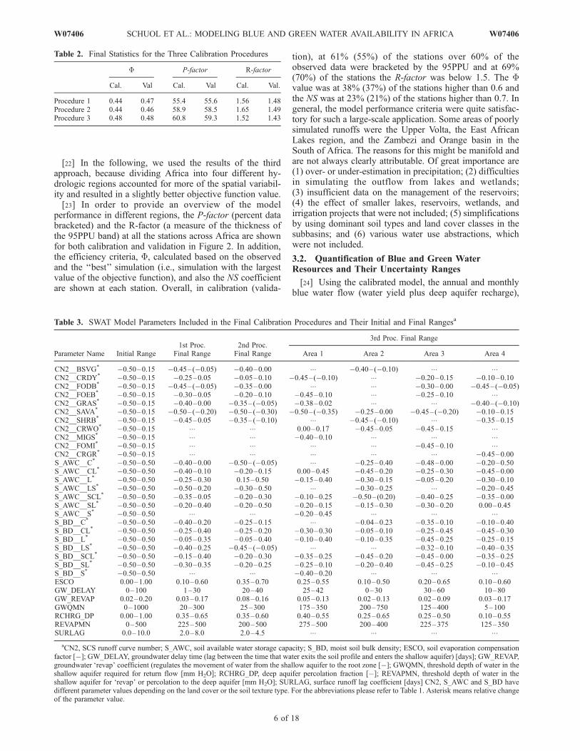
performance in different regions, the P-factor (percent databracketed) and the R-factor (a measure of the thickness ofthe 95PPU band) at all the stations across Africa are shownfor both calibration and validation in Figure 2. In addition,the efficiency criteria, F, calculated based on the observedand the ‘‘best’’ simulation (i.e., simulation with the largestvalue of the objective function), and also the NS coefficientare shown at each station. Overall, in calibration (valida-

tion), at 61% (55%) of the stations over 60% of theobserved data were bracketed by the 95PPU and at 69%(70%) of the stations the R-factor was below 1.5. The Fvalue was at 38% (37%) of the stations higher than 0.6 andthe NS was at 23% (21%) of the stations higher than 0.7. Ingeneral, the model performance criteria were quite satisfac-tory for such a large-scale application. Some areas of poorlysimulated runoffs were the Upper Volta, the East AfricanLakes region, and the Zambezi and Orange basin in theSouth of Africa. The reasons for this might be manifold andare not always clearly attributable. Of great importance are(1) over- or under-estimation in precipitation; (2) difficultiesin simulating the outflow from lakes and wetlands;(3) insufficient data on the management of the reservoirs;(4) the effect of smaller lakes, reservoirs, wetlands, andirrigation projects that were not included; (5) simplificationsby using dominant soil types and land cover classes in thesubbasins; and (6) various water use abstractions, whichwere not included.

3.2. Quantification of Blue and Green WaterResources and Their Uncertainty Ranges

[24] Using the calibrated model, the annual and monthlyblue water flow (water yield plus deep aquifer recharge),

Table 2. Final Statistics for the Three Calibration Procedures

F P-factor R-factor

Cal. Val Cal. Val Cal. Val.

Procedure 1 0.44 0.47 55.4 55.6 1.56 1.48Procedure 2 0.44 0.46 58.9 58.5 1.65 1.49Procedure 3 0.48 0.48 60.8 59.3 1.52 1.43

Table 3. SWAT Model Parameters Included in the Final Calibration Procedures and Their Initial and Final Rangesa

Parameter Name Initial Range1st Proc.

Final Range2nd Proc.

Final Range

3rd Proc. Final Range

Area 1 Area 2 Area 3 Area 4

CN2__BSVG* �0.50–0.15 �0.45– (�0.05) �0.40–0.00 �� 0.40– (�0.10) �� CN2__CRDY* �0.50–0.15 �0.25–0.05 �0.05–0.10 �0.45–(�0.10) �� 0.20–0.15 �0.10–0.10CN2__FODB* �0.50–0.15 �0.45– (�0.05) �0.35–0.00 �� 0.30–0.00 �0.45– (�0.05)CN2__FOEB* �0.50–0.15 �0.30–0.05 �0.20–0.10 �0.45–0.10 �� 0.25–0.10 ��CN2__GRAS* �0.50–0.15 �0.40–0.00 �0.35– (�0.05) �0.38–0.02 �� 0.40– (�0.10)CN2__SAVA* �0.50–0.15 �0.50– (�0.20) �0.50– (�0.30) �0.50–(�0.35) �0.25–0.00 �0.45–(�0.20) �0.10–0.15CN2__SHRB* �0.50–0.15 �0.45–0.05 �0.35– (�0.10) �� 0.45– (�0.10) �� 0.35–0.15CN2__CRWO* �0.50–0.15 �� 0.00–0.17 �0.45–0.05 �0.45–0.15 ��CN2__MIGS* �0.50–0.15 �� 0.40–0.10 �� CN2__FOMI* �0.50–0.15 �� 0.45–0.10 ��CN2__CRGR* �0.50–0.15 �� 0.45–0.00S_AWC__C* �0.50–0.50 �0.40–0.00 �0.50– (�0.05) �� 0.25–0.40 �0.48–0.00 �0.20–0.50S_AWC__CL* �0.50–0.50 �0.40–0.10 �0.20–0.15 0.00–0.45 �0.45–0.20 �0.25–0.30 �0.45–0.00S_AWC__L* �0.50–0.50 �0.25–0.30 0.15–0.50 �0.15–0.40 �0.30–0.15 �0.05–0.20 �0.30–0.10S_AWC__LS* �0.50–0.50 �0.50–0.20 �0.30–0.50 �� 0.30–0.25 �� 0.20–0.45S_AWC__SCL* �0.50–0.50 �0.35–0.05 �0.20–0.30 �0.10–0.25 �0.50– (0.20) �0.40–0.25 �0.35–0.00S_AWC__SL* �0.50–0.50 �0.20–0.40 �0.20–0.50 �0.20–0.15 �0.15–0.30 �0.30–0.20 0.00–0.45S_AWC__S* �0.50–0.50 �� 0.20–0.45 �� S_BD__C* �0.50–0.50 �0.40–0.20 �0.25–0.15 �� 0.04–0.23 �0.35–0.10 �0.10–0.40S_BD__CL* �0.50–0.50 �0.25–0.40 �0.25–0.20 �0.30–0.30 �0.05–0.10 �0.25–0.45 �0.45–0.30S_BD__L* �0.50–0.50 �0.05–0.35 �0.05–0.40 �0.10–0.40 �0.10–0.35 �0.45–0.25 �0.25–0.15S_BD__LS* �0.50–0.50 �0.40–0.25 �0.45– (�0.05) �� 0.32–0.10 �0.40–0.35S_BD__SCL* �0.50–0.50 �0.15–0.40 �0.20–0.30 �0.35–0.25 �0.45–0.20 �0.45–0.00 �0.35–0.25S_BD__SL* �0.50–0.50 �0.30–0.35 �0.20–0.25 �0.25–0.10 �0.20–0.40 �0.45–0.25 �0.10–0.45S_BD__S* �0.50–0.50 �� 0.40–0.20 �� ESCO 0.00–1.00 0.10–0.60 0.35–0.70 0.25–0.55 0.10–0.50 0.20–0.65 0.10–0.60GW_DELAY 0–100 1–30 20–40 25–42 0–30 30–60 10–80GW_REVAP 0.02–0.20 0.03–0.17 0.08–0.16 0.05–0.13 0.02–0.13 0.02–0.09 0.03–0.17GWQMN 0–1000 20–300 25–300 175–350 200–750 125–400 5–100RCHRG_DP 0.00–1.00 0.35–0.65 0.35–0.60 0.40–0.55 0.25–0.65 0.25–0.50 0.10–0.55REVAPMN 0–500 225–500 200–500 275–500 200–400 225–375 125–350SURLAG 0.0–10.0 2.0–8.0 2.0–4.5 ��

aCN2, SCS runoff curve number; S_AWC, soil available water storage capacity; S_BD, moist soil bulk density; ESCO, soil evaporation compensationfactor [�]; GW_DELAY, groundwater delay time (lag between the time that water exits the soil profile and enters the shallow aquifer) [days]; GW_REVAP,groundwater ‘revap’ coefficient (regulates the movement of water from the shallow aquifer to the root zone [�]; GWQMN, threshold depth of water in theshallow aquifer required for return flow [mm H2O]; RCHRG_DP, deep aquifer percolation fraction [�]; REVAPMN, threshold depth of water in theshallow aquifer for ‘revap’ or percolation to the deep aquifer [mm H2O]; SURLAG, surface runoff lag coefficient [days] CN2, S_AWC and S_BD havedifferent parameter values depending on the land cover or the soil texture type. For the abbreviations please refer to Table 1. Asterisk means relative changeof the parameter value.

6 of 18


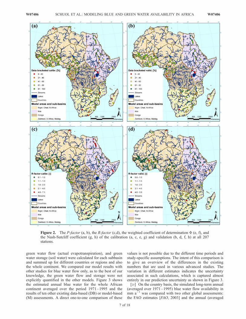
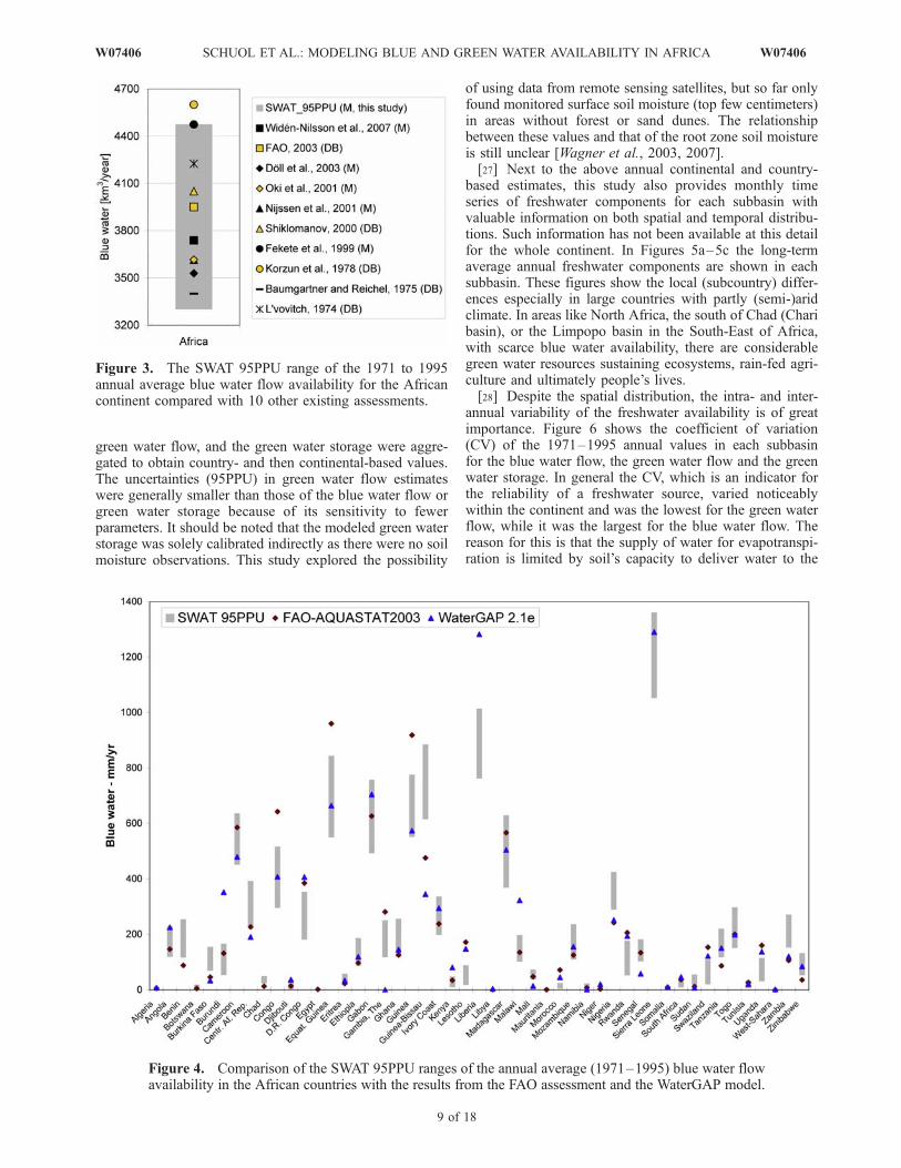
green water flow (actual evapotranspiration), and greenwater storage (soil water) were calculated for each subbasinand summed up for different countries or regions and alsothe whole continent. We compared our model results withother studies for blue water flow only, as to the best of ourknowledge, the green water flow and storage were notexplicitly quantified in the other models. Figure 3 showsthe estimated annual blue water for the whole Africancontinent averaged over the period 1971–1995 and theresults of ten other existing data-based (DB) or model-based(M) assessments. A direct one-to-one comparison of these

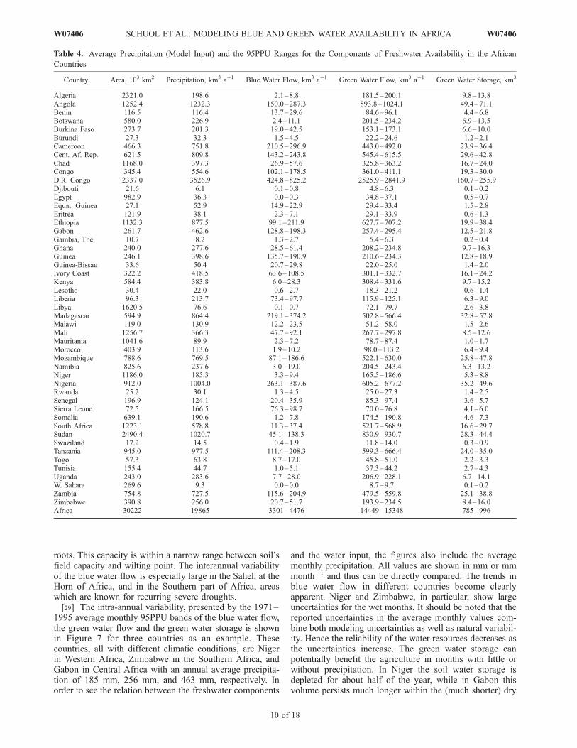
values is not possible due to the different time periods andstudy-specific assumptions. The intent of this comparison isto give an overview of the differences in the existingnumbers that are used in various advanced studies. Thevariation in different estimates indicates the uncertaintyassociated in such calculations, which is captured almostentirely in our prediction uncertainty as shown in Figure 3.[25] On the country basis, the simulated long-term annual

(averaged over 1971–1995) blue water flow availability inmm a�1 was compared with two other global assessments:the FAO estimates [FAO, 2003] and the annual (averaged

Figure 2. The P-factor (a, b), the R-factor (c,d), the weighted coefficient of determination F (e, f), andthe Nash-Sutcliff coefficient (g, h) of the calibration (a, c, e, g) and validation (b, d, f, h) at all 207stations.


7 of 18

W07406

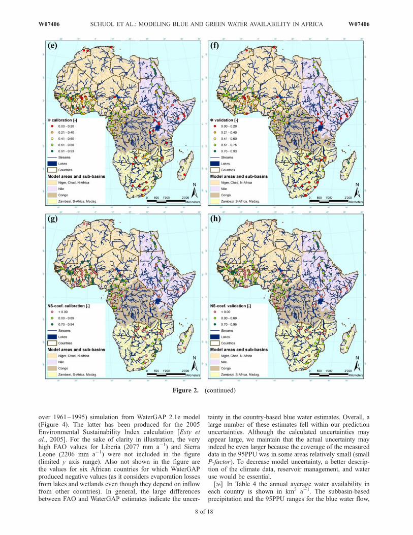
over 1961–1995) simulation from WaterGAP 2.1e model(Figure 4). The latter has been produced for the 2005Environmental Sustainability Index calculation [Esty etal., 2005]. For the sake of clarity in illustration, the veryhigh FAO values for Liberia (2077 mm a�1) and SierraLeone (2206 mm a�1) were not included in the figure(limited y axis range). Also not shown in the figure arethe values for six African countries for which WaterGAPproduced negative values (as it considers evaporation lossesfrom lakes and wetlands even though they depend on inflowfrom other countries). In general, the large differencesbetween FAO and WaterGAP estimates indicate the uncer-

tainty in the country-based blue water estimates. Overall, alarge number of these estimates fell within our predictionuncertainties. Although the calculated uncertainties mayappear large, we maintain that the actual uncertainty mayindeed be even larger because the coverage of the measureddata in the 95PPU was in some areas relatively small (smallP-factor). To decrease model uncertainty, a better descrip-tion of the climate data, reservoir management, and wateruse would be essential.[26] In Table 4 the annual average water availability in

each country is shown in km3 a�1. The subbasin-basedprecipitation and the 95PPU ranges for the blue water flow,

Figure 2. (continued)

8 of 18


green water flow, and the green water storage were aggre-gated to obtain country- and then continental-based values.The uncertainties (95PPU) in green water flow estimateswere generally smaller than those of the blue water flow orgreen water storage because of its sensitivity to fewerparameters. It should be noted that the modeled green waterstorage was solely calibrated indirectly as there were no soilmoisture observations. This study explored the possibility

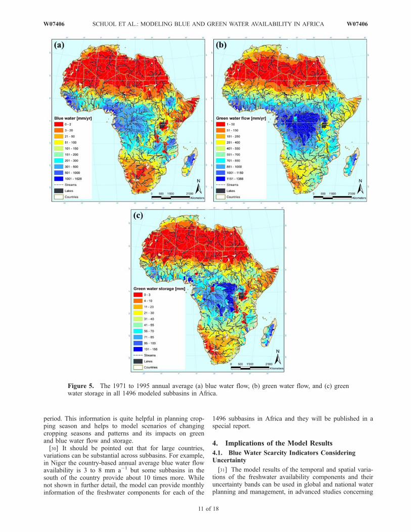
of using data from remote sensing satellites, but so far onlyfound monitored surface soil moisture (top few centimeters)in areas without forest or sand dunes. The relationshipbetween these values and that of the root zone soil moistureis still unclear [Wagner et al., 2003, 2007].[27] Next to the above annual continental and country-

based estimates, this study also provides monthly timeseries of freshwater components for each subbasin withvaluable information on both spatial and temporal distribu-tions. Such information has not been available at this detailfor the whole continent. In Figures 5a–5c the long-termaverage annual freshwater components are shown in eachsubbasin. These figures show the local (subcountry) differ-ences especially in large countries with partly (semi-)aridclimate. In areas like North Africa, the south of Chad (Charibasin), or the Limpopo basin in the South-East of Africa,with scarce blue water availability, there are considerablegreen water resources sustaining ecosystems, rain-fed agri-culture and ultimately people’s lives.[28] Despite the spatial distribution, the intra- and inter-

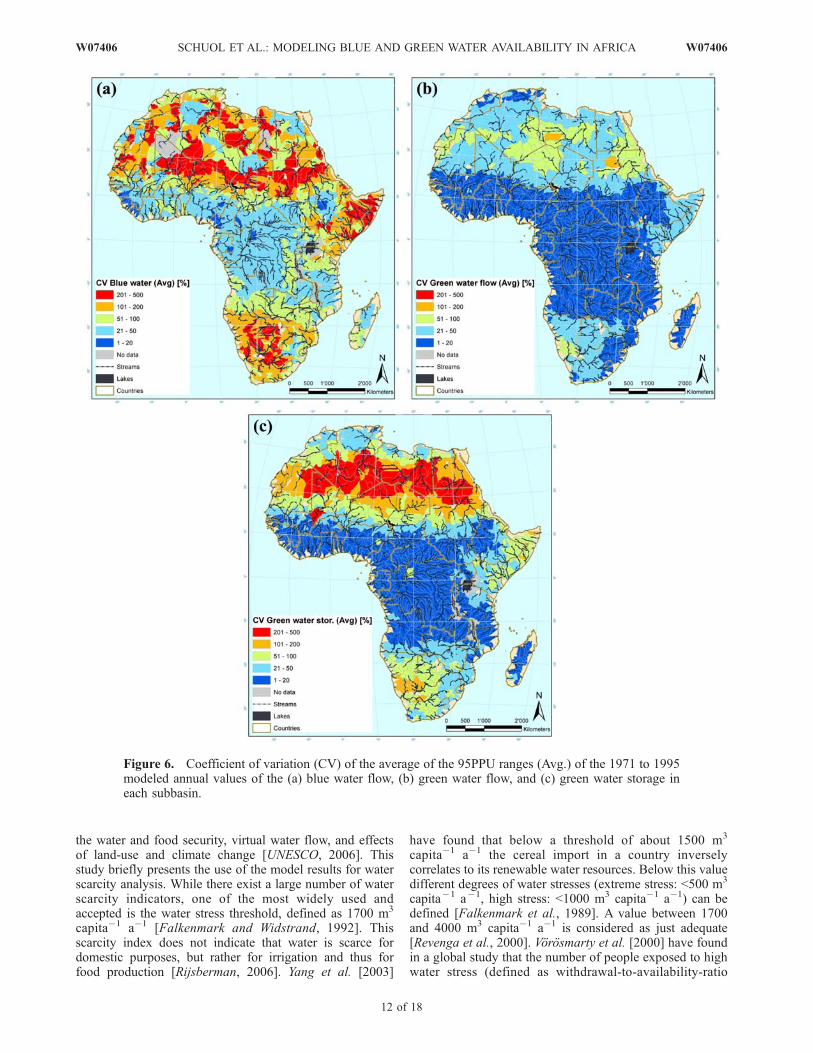
annual variability of the freshwater availability is of greatimportance. Figure 6 shows the coefficient of variation(CV) of the 1971–1995 annual values in each subbasinfor the blue water flow, the green water flow and the greenwater storage. In general the CV, which is an indicator forthe reliability of a freshwater source, varied noticeablywithin the continent and was the lowest for the green waterflow, while it was the largest for the blue water flow. Thereason for this is that the supply of water for evapotranspi-ration is limited by soil’s capacity to deliver water to the

Figure 3. The SWAT 95PPU range of the 1971 to 1995annual average blue water flow availability for the Africancontinent compared with 10 other existing assessments.

Figure 4. Comparison of the SWAT 95PPU ranges of the annual average (1971–1995) blue water flowavailability in the African countries with the results from the FAO assessment and the WaterGAP model.


9 of 18

W07406

roots. This capacity is within a narrow range between soil’sfield capacity and wilting point. The interannual variabilityof the blue water flow is especially large in the Sahel, at theHorn of Africa, and in the Southern part of Africa, areaswhich are known for recurring severe droughts.[29] The intra-annual variability, presented by the 1971–

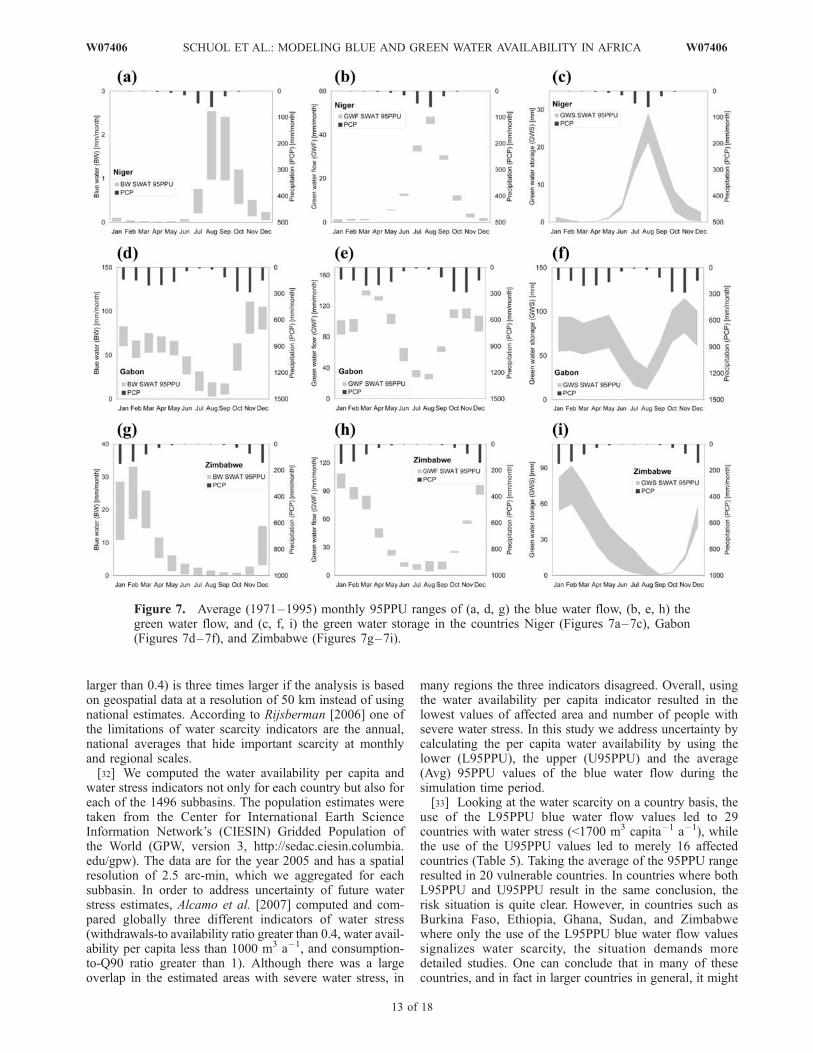
1995 average monthly 95PPU bands of the blue water flow,the green water flow and the green water storage is shownin Figure 7 for three countries as an example. Thesecountries, all with different climatic conditions, are Nigerin Western Africa, Zimbabwe in the Southern Africa, andGabon in Central Africa with an annual average precipita-tion of 185 mm, 256 mm, and 463 mm, respectively. Inorder to see the relation between the freshwater components

and the water input, the figures also include the averagemonthly precipitation. All values are shown in mm or mmmonth�1 and thus can be directly compared. The trends inblue water flow in different countries become clearlyapparent. Niger and Zimbabwe, in particular, show largeuncertainties for the wet months. It should be noted that thereported uncertainties in the average monthly values com-bine both modeling uncertainties as well as natural variabil-ity. Hence the reliability of the water resources decreases asthe uncertainties increase. The green water storage canpotentially benefit the agriculture in months with little orwithout precipitation. In Niger the soil water storage isdepleted for about half of the year, while in Gabon thisvolume persists much longer within the (much shorter) dry

Table 4. Average Precipitation (Model Input) and the 95PPU Ranges for the Components of Freshwater Availability in the African

Countries

Country Area, 103 km2 Precipitation, km3 a�1 Blue Water Flow, km3 a�1 Green Water Flow, km3 a�1 Green Water Storage, km3

Algeria 2321.0 198.6 2.1–8.8 181.5–200.1 9.8–13.8Angola 1252.4 1232.3 150.0–287.3 893.8–1024.1 49.4–71.1Benin 116.5 116.4 13.7–29.6 84.6–96.1 4.4–6.8Botswana 580.0 226.9 2.4–11.1 201.5–234.2 6.9–13.5Burkina Faso 273.7 201.3 19.0–42.5 153.1–173.1 6.6–10.0Burundi 27.3 32.3 1.5–4.5 22.2–24.6 1.2–2.1Cameroon 466.3 751.8 210.5–296.9 443.0–492.0 23.9–36.4Cent. Af. Rep. 621.5 809.8 143.2–243.8 545.4–615.5 29.6–42.8Chad 1168.0 397.3 26.9–57.6 325.8–363.2 16.7–24.0Congo 345.4 554.6 102.1–178.5 361.0–411.1 19.3–30.0D.R. Congo 2337.0 3526.9 424.8–825.2 2525.9–2841.9 160.7–255.9Djibouti 21.6 6.1 0.1–0.8 4.8–6.3 0.1–0.2Egypt 982.9 36.3 0.0–0.3 34.8–37.1 0.5–0.7Equat. Guinea 27.1 52.9 14.9–22.9 29.4–33.4 1.5–2.8Eritrea 121.9 38.1 2.3–7.1 29.1–33.9 0.6–1.3Ethiopia 1132.3 877.5 99.1–211.9 627.7–707.2 19.9–38.4Gabon 261.7 462.6 128.8–198.3 257.4–295.4 12.5–21.8Gambia, The 10.7 8.2 1.3–2.7 5.4–6.3 0.2–0.4Ghana 240.0 277.6 28.5–61.4 208.2–234.8 9.7–16.3Guinea 246.1 398.6 135.7–190.9 210.6–234.3 12.8–18.9Guinea-Bissau 33.6 50.4 20.7–29.8 22.0–25.0 1.4–2.0Ivory Coast 322.2 418.5 63.6–108.5 301.1–332.7 16.1–24.2Kenya 584.4 383.8 6.0–28.3 308.4–331.6 9.7–15.2Lesotho 30.4 22.0 0.6–2.7 18.3–21.2 0.6–1.4Liberia 96.3 213.7 73.4–97.7 115.9–125.1 6.3–9.0Libya 1620.5 76.6 0.1–0.7 72.1–79.7 2.6–3.8Madagascar 594.9 864.4 219.1–374.2 502.8–566.4 32.8–57.8Malawi 119.0 130.9 12.2–23.5 51.2–58.0 1.5–2.6Mali 1256.7 366.3 47.7–92.1 267.7–297.8 8.5–12.6Mauritania 1041.6 89.9 2.3–7.2 78.7–87.4 1.0–1.7Morocco 403.9 113.6 1.9–10.2 98.0–113.2 6.4–9.4Mozambique 788.6 769.5 87.1–186.6 522.1–630.0 25.8–47.8Namibia 825.6 237.6 3.0–19.0 204.5–243.4 6.3–13.2Niger 1186.0 185.3 3.3–9.4 165.5–186.6 5.3–8.8Nigeria 912.0 1004.0 263.1–387.6 605.2–677.2 35.2–49.6Rwanda 25.2 30.1 1.3–4.5 25.0–27.3 1.4–2.5Senegal 196.9 124.1 20.4–35.9 85.3–97.4 3.6–5.7Sierra Leone 72.5 166.5 76.3–98.7 70.0–76.8 4.1–6.0Somalia 639.1 190.6 1.2–7.8 174.5–190.8 4.6–7.3South Africa 1223.1 578.8 11.3–37.4 521.7–568.9 16.6–29.7Sudan 2490.4 1020.7 45.1–138.3 830.9–930.7 28.3–44.4Swaziland 17.2 14.5 0.4–1.9 11.8–14.0 0.3–0.9Tanzania 945.0 977.5 111.4–208.3 599.3–666.4 24.0–35.0Togo 57.3 63.8 8.7–17.0 45.8–51.0 2.2–3.3Tunisia 155.4 44.7 1.0–5.1 37.3–44.2 2.7–4.3Uganda 243.0 283.6 7.7–28.0 206.9–228.1 6.7–14.1W. Sahara 269.6 9.3 0.0–0.0 8.7–9.7 0.1–0.2Zambia 754.8 727.5 115.6–204.9 479.5–559.8 25.1–38.8Zimbabwe 390.8 256.0 20.7–51.7 193.9–234.5 8.4–16.0Africa 30222 19865 3301–4476 14449–15348 785–996

10 of 18


period. This information is quite helpful in planning crop-ping season and helps to model scenarios of changingcropping seasons and patterns and its impacts on greenand blue water flow and storage.[30] It should be pointed out that for large countries,

variations can be substantial across subbasins. For example,in Niger the country-based annual average blue water flowavailability is 3 to 8 mm a�1 but some subbasins in thesouth of the country provide about 10 times more. Whilenot shown in further detail, the model can provide monthlyinformation of the freshwater components for each of the

1496 subbasins in Africa and they will be published in aspecial report.

4. Implications of the Model Results

4.1. Blue Water Scarcity Indicators ConsideringUncertainty

[31] The model results of the temporal and spatial varia-tions of the freshwater availability components and theiruncertainty bands can be used in global and national waterplanning and management, in advanced studies concerning

Figure 5. The 1971 to 1995 annual average (a) blue water flow, (b) green water flow, and (c) greenwater storage in all 1496 modeled subbasins in Africa.


11 of 18

W07406

the water and food security, virtual water flow, and effectsof land-use and climate change [UNESCO, 2006]. Thisstudy briefly presents the use of the model results for waterscarcity analysis. While there exist a large number of waterscarcity indicators, one of the most widely used andaccepted is the water stress threshold, defined as 1700 m3

capita�1 a�1 [Falkenmark and Widstrand, 1992]. Thisscarcity index does not indicate that water is scarce fordomestic purposes, but rather for irrigation and thus forfood production [Rijsberman, 2006]. Yang et al. [2003]

have found that below a threshold of about 1500 m3

capita�1 a�1 the cereal import in a country inverselycorrelates to its renewable water resources. Below this valuedifferent degrees of water stresses (extreme stress: <500 m3

capita�1 a�1, high stress: <1000 m3 capita�1 a�1) can bedefined [Falkenmark et al., 1989]. A value between 1700and 4000 m3 capita�1 a�1 is considered as just adequate[Revenga et al., 2000]. Vorosmarty et al. [2000] have foundin a global study that the number of people exposed to highwater stress (defined as withdrawal-to-availability-ratio

Figure 6. Coefficient of variation (CV) of the average of the 95PPU ranges (Avg.) of the 1971 to 1995modeled annual values of the (a) blue water flow, (b) green water flow, and (c) green water storage ineach subbasin.

12 of 18


larger than 0.4) is three times larger if the analysis is basedon geospatial data at a resolution of 50 km instead of usingnational estimates. According to Rijsberman [2006] one ofthe limitations of water scarcity indicators are the annual,national averages that hide important scarcity at monthlyand regional scales.[32] We computed the water availability per capita and

water stress indicators not only for each country but also foreach of the 1496 subbasins. The population estimates weretaken from the Center for International Earth ScienceInformation Network’s (CIESIN) Gridded Population ofthe World (GPW, version 3, http://sedac.ciesin.columbia.edu/gpw). The data are for the year 2005 and has a spatialresolution of 2.5 arc-min, which we aggregated for eachsubbasin. In order to address uncertainty of future waterstress estimates, Alcamo et al. [2007] computed and com-pared globally three different indicators of water stress(withdrawals-to availability ratio greater than 0.4, water avail-ability per capita less than 1000 m3 a�1, and consumption-to-Q90 ratio greater than 1). Although there was a largeoverlap in the estimated areas with severe water stress, in

many regions the three indicators disagreed. Overall, usingthe water availability per capita indicator resulted in thelowest values of affected area and number of people withsevere water stress. In this study we address uncertainty bycalculating the per capita water availability by using thelower (L95PPU), the upper (U95PPU) and the average(Avg) 95PPU values of the blue water flow during thesimulation time period.[33] Looking at the water scarcity on a country basis, the

use of the L95PPU blue water flow values led to 29countries with water stress (<1700 m3 capita�1 a�1), whilethe use of the U95PPU values led to merely 16 affectedcountries (Table 5). Taking the average of the 95PPU rangeresulted in 20 vulnerable countries. In countries where bothL95PPU and U95PPU result in the same conclusion, therisk situation is quite clear. However, in countries such asBurkina Faso, Ethiopia, Ghana, Sudan, and Zimbabwewhere only the use of the L95PPU blue water flow valuessignalizes water scarcity, the situation demands moredetailed studies. One can conclude that in many of thesecountries, and in fact in larger countries in general, it might

Figure 7. Average (1971–1995) monthly 95PPU ranges of (a, d, g) the blue water flow, (b, e, h) thegreen water flow, and (c, f, i) the green water storage in the countries Niger (Figures 7a–7c), Gabon(Figures 7d–7f), and Zimbabwe (Figures 7g–7i).


13 of 18

W07406

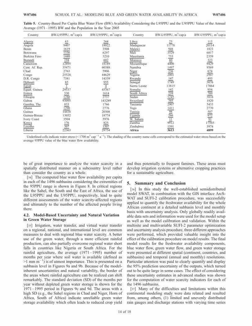
be of great importance to analyze the water scarcity in aspatially distributed manner on a subcountry level ratherthan consider the country as a whole.[34] The computed blue water flow availability per capita

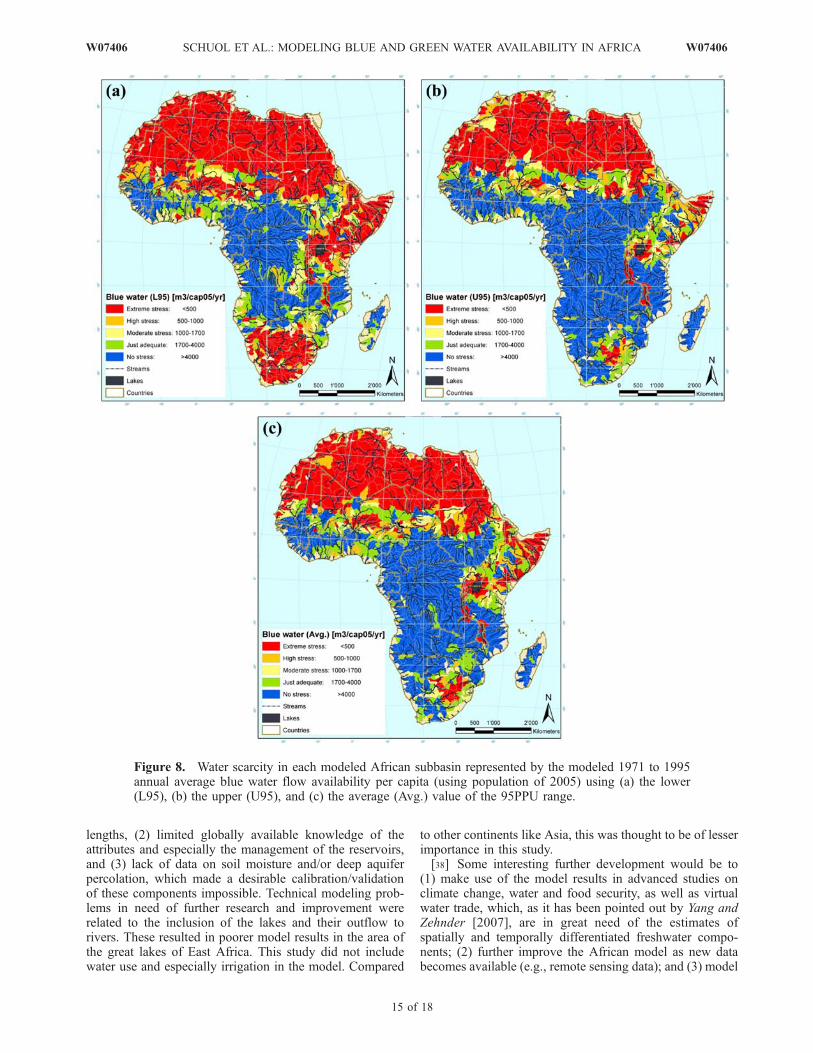
in each of the 1496 subbasins considering the extremities ofthe 95PPU range is shown in Figure 8. In critical regionslike the Sahel, the South and the East of Africa, the use ofthe L95PPU and the U95PPU, respectively, lead to quitedifferent assessments of the water scarcity-affected regionsand ultimately to the number of the affected people livingthere.

4.2. Model-Based Uncertainty and Natural Variationin Green Water Storage

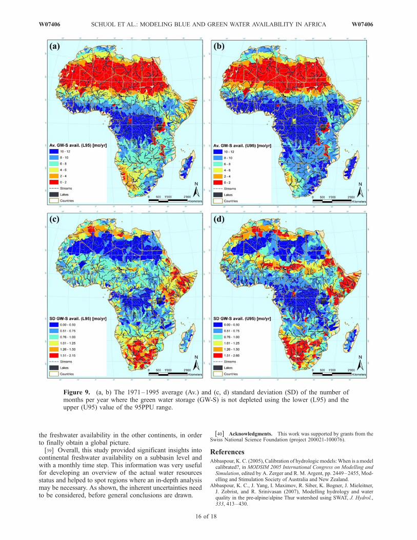
[35] Irrigation, water transfer, and virtual water transferon a regional, national, and international level are commonmeasures to deal with regional blue water scarcity. A betteruse of the green water, through a more efficient rainfedproduction, can also partially overcome regional water shortfalls in countries like Nigeria or South Africa. For therainfed agriculture, the average (1971–1995) number ofmonths per year where soil water is available (defined as>1 mm m�1) is of utmost importance. This is presented on asubbasin level in Figures 9a and 9b. Because of the model-inherent uncertainties and natural variability, the border ofthe areas where rainfed agriculture can be realized can shiftremarkably. The standard deviation (SD) of the months peryear without depleted green water storage is shown for the1971–1995 period in Figures 9c and 9d. The areas with ahigh SD (e.g., the Sahel regions in Chad and Niger, Horn ofAfrica, South of Africa) indicate unreliable green waterstorage availability which often leads to reduced crop yield

and thus potentially to frequent famines. These areas mustdevelop irrigation systems or alternative cropping practicesfor a sustainable agriculture.

5. Summary and Conclusion

[36] In this study the well-established semidistributedmodel SWAT, in combination with the GIS interface ArcS-WAT and SUFI-2 calibration procedure, was successfullyapplied to quantify the freshwater availability for the wholeAfrican continent at a detailed subbasin level and monthlybasis with uncertainty analysis. Only globally readily avail-able data sets and information were used for the model setupas well as the model calibration and validation. Within themultisite and multivariable SUFI-2 parameter optimizationand uncertainty analysis procedure, three different approacheswere performed, which provided valuable insight into theeffect of the calibration procedure on model results. The finalmodel results for the freshwater availability components,blue water flow, green water flow, and green water storagewere presented at different spatial (continent, countries, andsubbasins) and temporal (annual and monthly) resolutions.Particular attention was paid to clearly quantify and displaythe 95% prediction uncertainty of the outputs, which turnedout to be quite large in some cases. The effect of consideringthese uncertainty estimates in advanced studies was shownfor the computation of water scarcity indicators for each ofthe 1496 subbasins.[37] Many of the difficulties and limitations within this

continental modeling study were data related and resultedfrom, among others, (1) limited and unevenly distributedrain gauges and discharge stations with varying time series

Table 5. Country-Based Per Capita Blue Water Flow (BW) Availability Considering the L95PPU and the U95PPU Value of the Annual

Average (1971–1995) BW and the Population in the Year 2005

Country BW-L95PPU, m3/cap/a BW-U95PPU, m3/cap/a Country BW-L95PPU, m3/cap/a BW-U95PPU, m3/cap/a

Algeria 63 268 Libya 23 113Angola 9407 18022 Madagascar 11778 20114Benin 1619 3508 Malawi 948 1823Botswana 1336 6297 Mali 3529 6817Burkina Faso 1440 3210 Mauritania 733 2359Burundi 194 602 Morocco 60 323Cameroon 12895 18189 Mozambique 4400 9429Cent. Af. Rep. 35471 60388 Namibia 1497 9369Chad 2763 5906 Niger 236 674Congo 25528 44629 Nigeria 2001 2947D.R. Congo 7381 14339 Rwanda 147 493Djibouti 85 955 Senegal 1749 3076Egypt 1 4 Sierra Leone 13815 17864Equat. Guinea 29537 45367 Somalia 142 954Eritrea 530 1614 South Africa 239 789Ethiopia 1280 2737 Sudan 1245 3816Gabon 93095 143289 Swaziland 345 1820Gambia, The 833 1766 Tanzania 2907 5433Ghana 1290 2776 Togo 1411 2770Guinea 14438 20308 Tunisia 98 507Guinea-Bissau 13052 18774 Uganda 266 972Ivory Coast 3504 5976 W. Sahara 11 91Kenya 176 825 Zambia 9912 17565Lesotho 307 1507 Zimbabwe 1591 3974Liberia 22363 29754 Africa 3613 4899

Underlined cells indicate water stress (< 1700 m3 cap�1 a�1). The shading of the country name cells correspond to the estimated water stress based on theaverage 95PPU value of the blue water flow availability.

14 of 18


lengths, (2) limited globally available knowledge of theattributes and especially the management of the reservoirs,and (3) lack of data on soil moisture and/or deep aquiferpercolation, which made a desirable calibration/validationof these components impossible. Technical modeling prob-lems in need of further research and improvement wererelated to the inclusion of the lakes and their outflow torivers. These resulted in poorer model results in the area ofthe great lakes of East Africa. This study did not includewater use and especially irrigation in the model. Compared

to other continents like Asia, this was thought to be of lesserimportance in this study.[38] Some interesting further development would be to

(1) make use of the model results in advanced studies onclimate change, water and food security, as well as virtualwater trade, which, as it has been pointed out by Yang andZehnder [2007], are in great need of the estimates ofspatially and temporally differentiated freshwater compo-nents; (2) further improve the African model as new databecomes available (e.g., remote sensing data); and (3) model

Figure 8. Water scarcity in each modeled African subbasin represented by the modeled 1971 to 1995annual average blue water flow availability per capita (using population of 2005) using (a) the lower(L95), (b) the upper (U95), and (c) the average (Avg.) value of the 95PPU range.


15 of 18

W07406

the freshwater availability in the other continents, in orderto finally obtain a global picture.[39] Overall, this study provided significant insights into

continental freshwater availability on a subbasin level andwith a monthly time step. This information was very usefulfor developing an overview of the actual water resourcesstatus and helped to spot regions where an in-depth analysismay be necessary. As shown, the inherent uncertainties needto be considered, before general conclusions are drawn.

[40] Acknowledgments. This work was supported by grants from theSwiss National Science Foundation (project 200021-100076).

ReferencesAbbaspour, K. C. (2005), Calibration of hydrologic models:When is a modelcalibrated?, in MODSIM 2005 International Congress on Modelling andSimulation, edited by A. Zerger and R. M. Argent, pp. 2449–2455, Mod-elling and Stimulation Society of Australia and New Zealand.

Abbaspour, K. C., J. Yang, I. Maximov, R. Siber, K. Bogner, J. Mieleitner,J. Zobrist, and R. Srinivasan (2007), Modelling hydrology and waterquality in the pre-alpine/alpine Thur watershed using SWAT, J. Hydrol.,333, 413–430.

Figure 9. (a, b) The 1971–1995 average (Av.) and (c, d) standard deviation (SD) of the number ofmonths per year where the green water storage (GW-S) is not depleted using the lower (L95) and theupper (U95) value of the 95PPU range.

16 of 18


Abbaspour, K. C., J. Yang, M. Vejdani, and S. Haghighat (2008), SWAT-CUP: Calibration and uncertainty programs for SWAT, 4th Int. SWATConf. Proc., in press.

Alcamo, J., P. Doll, T. Henrichs, F. Kaspar, B. Lehner, T. Rosch, andS. Siebert (2003), Development and testing of the WaterGAP 2 globalmodel of water use and availability, Hydrol. Sci. J., 48(3), 317–337.

Alcamo, J., M. Florke, and M. Marker (2007), Future long-term changes inglobal water resources driven by socio-economic and climatic changes,Hydrol. Sci. J., 52(2), 247–275.

Arnell, N. W. (1999), Climate change and global water resources, GlobalEnviron. Change, 9, S31–S49.

Arnold, J. G., R. Srinivasan, R. S. Muttiah, and J. R. Williams (1998),Large area hydrologic modeling and assessment. Part I: Model develop-ment, J. Am. Water Resour. Assoc., 34(1), 73–89.

Arnold, J. G., R. Srinivasan, R. S. Muttiah, and P. M. Allen (1999), Con-tinental scale simulation of the hydrologic balance, J. Am. Water Resour.Assoc., 35(5), 1037–1051.

Baumgartner, A., and E. Reichel (1975), The World Water Balance, 182 pp.,Elsevier, New York.

Beven, K., and A. Binley (1992), The future of distributed models - Modelcalibration and uncertainty prediction, Hydrol. Processes, 6(3), 279–298.

Butts, M. B., J. T. Payne, M. Kristensen, and H. Madsen (2004), Anevaluation of the impact of model structure on hydrological modellinguncertainty for streamflow simulation, J. Hydrol., 298(1–4), 242–266.

Di Luzio, M., R. Srinivasan, and J. G. Arnold (2001), ArcView Interface forSWAT2000 - User’s Guide, Blackland Research Center, Texas Agricul-tural Experiment Station and Grassland, Soil and Water ResearchLaboratory, USDA Agricultural Research Service, Temple, Tex.

Doll, P., F. Kaspar, and B. Lehner (2003), A global hydrological model forderiving water availability indicators: Model tuning and validation,J. Hydrol., 270(1–2), 105–134.

Esty, D. C., M. Levy, T. Srebotnjak, and A. de Sherbinin (2005), 2005Environmental Sustainability Index: Benchmarking National Environ-mental Stewardship, Yale Center for Environ. Law & Policy, New Haven,USA.

Falkenmark, M. (1989), The massive water scarcity now threateningAfrice - Why isn’t it being addressed?, AMBIO, 18(2), 112–118.

Falkenmark, M., and J. Rockstrom (2006), The new blue and green waterparadigm: Breaking new ground for water resources planning and man-agement, J. Water Resour. Plann. Manage., 132(3), 129–132.

Falkenmark, M., and C. Widstrand (1992), Population and water resources:A delicate balance, Popul. Bull., 47(3), 1–36.

Falkenmark, M., J. Lundquist, and C. Widstrand (1989), Macro-scale waterscarcity requires micro-scale approaches: Aspects of vulnerability insemi-arid development, Nat. Resour. Forum, 13, 258–267.

FAO (Food and Agriculture Organization) (1995), Digital soil map of theworld and derived soil properties [CD-ROM], Version 3.5, Land andWater Digital Media Series Number 1, Rome, Italy.

FAO (Food and Agriculture Organization) (2003), Review of the worldwater resources by country, Water Report 23, Rome, Italy. (Availableat ftp://ftp.fao.org/agl/aglw/docs/wr23e.pdf)

Fekete, B. M., C. J. Vorosmarty, and W. Grabs (1999), Global compositerunoff fields of observed river discharge and simulated water balances,Report No. 22, Global Runoff Data Centre, Koblenz, Germany.

Gassman, P. W., M. R. Reyes, C. H. Green, and J. G. Arnold (2007), Thesoil and water assessment tool: Historical development, applications, andfuture research directions, Trans. ASAE, 50(4), 1211–1250.

Gerten, D., S. Schaphoff, U. Haberlandt, W. Lucht, and S. Sitch (2004),Terrestrial vegetation and water balance - Hydrological evaluation of adynamic global vegetation model, J. Hydrol., 286, 249–270.

Gerten, D., H. Hoff, A. Bondeau, W. Lucht, P. Smith, and S. Zaehle (2005),Contemporary ‘‘green’’ water flows: Simulations with a dynamic globalvegetation and water balance model, Phys. Chem. Earth, 30, 334–338.

Guntner, A., J. Stuck, S. Werth, P. Doll, K. Verzano, and B. Merz (2007),A global analysis of temporal and spatial variations in continental waterstorage,Water Resour. Res., 43(5), W05416, doi:10.1029/2006WR005247.

Islam, M. S., T. Oki, S. Kanae, N. Hanasaki, Y. Agata, and K. Yoshimura(2007), A grid-based assessment of global water scarcity including vir-tual water trading, Water Resour. Manage., 21, 19–33.

Korzun, V. I., A. A. Sokolow, M. I. Budyko, K. P. Voskresensky, G. P.Kalinin, A. A. Konoplyanstev, E. S. Korotkevich, P. S. Kuzin, and M. I.L’vovich, (Eds.) (1978), World Water Balance and Water Resources ofthe Earth, UNESCO, Paris.

Krause, P., D. P. Boyle, and F. Base (2005), Comparison of different effi-ciency criteria for hydrological model assessment, Adv. Geosci., 5, 89–97.

Lehner, B., and P. Doll (2004), Development and validation of a globaldatabase of lakes, reservoirs and wetlands, J. Hydrol., 296(1–4), 1–22.

L’vovitch, M. I. (1974),World water resources and their future (in Russian),Moscow,Mysl. English translation: R. L. Nace (1979),Washington, D. C.,AGU, 415 pp.

Neitsch, S. L., J. G. Arnold, J. R. Kiniry, and J. R. Williams (2005), Soiland Water Assessment Tool - Theoretical Documentation - Version 2005,Grassland, Soil and Water Research Laboratory, Agricultural ResearchService and Blackland Research Center, Texas Agricultural ExperimentStation, Temple, Tex.

Nijssen, B., G. M. O’Donnell, D. P. Lettenmaier, D. Lohmann, and E. F.Wood (2001), Predicting the discharge of global rivers, J. Clim., 14(15),3307–3323.

Oki, T., and S. Kanae (2006), Global hydrological cycles and world waterresources, Science, 313, 1068–1072.

Oki, T., Y. Agata, S. Kanae, T. Saruhashi, D. W. Yang, and K. Musiake(2001), Global assessment of current water resources using total runoffintegrating pathways, Hydrol. Sci. J., 46(6), 983–995.

Revenga, C., J. Brunner, N. Henninger, K. Kassem, and R. Payne (2000),Pilot Analysis of Global Ecosystems: Freshwater Systems, World Resour.Inst., Washington, D.C., USA.

Rijsberman, F. R. (2006), Water scarcity: Fact or fiction?, Agric. WaterManage., 80, 5–22.

Rockstrom, J., and L. Gordon (2001), Assessment of green water flows tosustain major biomes of the world: Implications for future ecohydrolo-gical landscape management, Phys. Chem. Earth Part B, 26(11–12),843–851.

Rockstrom, J., M. Lannerstad, and M. Falkenmark (2007), Assessing thewater challenge of a new green revolution in developing countries,PNAS, 104(15), 6253–6260.

Savenije, H. H. G. (2004), The importance of interception and why weshould delete the term evapotranspiration from our vocabulary, Hydrol.Processes, 18, 1507–1511.

Schuol, J., and K. C. Abbaspour (2007), Using monthly weather statistics togenerate daily data in a SWAT model application to West Africa, Ecol.Modell., 201, 301–311.

Schuol, J., K. C. Abbaspour, R. Srinivasan, and H. Yang (2008), Estimationof freshwater availability in the West African sub-continent using theSWAT hydrologic model, J. Hydrol., 352, 30–49.

Shiklomanov, I. A. (2000), Appraisal and assessment of world water re-sources, Water Int., 25(1), 11–32.

Shiklomanov, I. A., and J. Rodda (Eds.) (2003), World Water Resources atthe Beginning of the 21st Century, Cambridge Univ. Press, New York.

Smakhtin, V., C. Revenga, and P. Doll (2004), Taking into account envir-onmental water requirements in global-scale water resources assess-ments, Comprehensive Assessment Research Report 2, InternationalWater Management Institute, Colombo, Sri Lanka.

Srinivasan, R., T. S. Ramanarayanan, J. G. Arnold, and S. T. Bednarz(1998), Large area hydrologic modeling and assessment. Part II: Modelapplication, J. Am. Water Resour. Assoc., 34(1), 91–101.

UNESCO (2006), Water a shared responsibility, The United Nations WorldWater Development Report 2, UNESCO-WWAP, Paris, France.

UN-Water/Africa (2006), African water development report 2006, Econ.Comm. for Afr., Addis Ababa.

van Griensven, A., and T. Meixner (2006), Methods to quantify and identifythe sources of uncertainty for river basin water quality models,Water Sci.Technol., 53(1), 51–59.

Vorosmarty, C. J., C. A. Federer, and A. L. Schloss (1998), Evaporationfunctions compared on US watersheds: Possible implications for global-scale water balance and terrestrial ecosystem modeling, J. Hydrol.,207(3–4), 147–169.

Vorosmarty, C. J., P. Green, J. Salisbury, and R. B. Lammers (2000), Globalwater resources: Vulnerability from climate change and populationgrowth, Science, 289, 284–288.

Vorosmarty, C. J., E. M. Douglas, P. A. Green, and C. Revenga (2005),Geospatial indicators of emerging water stress: An application to Africa,Ambio, 34(3), 230–236.

Vrugt, J. A., H. V. Gupta, W. Bouten, and S. Sorooshian (2003), A ShuffledComplex Evolution Metropolis algorithm for optimization and uncer-tainty assessment of hydrologic model parameters, Water Resour. Res.,39(8), 1201, doi:10.1029/2002WR001642.

Wagner, W., K. Scipal, C. Pathe, D. Gerten, W. Lucht, and B. Rudolf(2003), Evaluation of the agreement between the first global remotelysensed soil moisture data with model and precipitation data, J. Geophys.Res., 108(D19), 4611, doi:10.1029/2003JD003663.

Wagner, W., G. Bloschl, P. Pampaloni, J.-C. Calvet, B. Bizzarri, J.-P.Wigneron, and Y. Kerr (2007), Operational readiness of microwave re-


17 of 18

W07406

mote sensing of soil moisture for hydrologic applications, Nord. Hydrol.,38(1), 1–20.

Wallace, J. S., and P. J. Gregory (2002), Water resources and their use infood production systems, Aquat. Sci., 64, 363–375.

Widen-Nilsson, E., S. Halldin, and C.-Y. Xu (2007), Global water-balancemodelling with WASMOD-M: Parameter estimation and regionalisation,J. Hydrol., 340, 105–118.

Winchell, M., R. Srinivasan, M. Di Luzio, and J. G. Arnold (2007), Arc-SWAT interface for SWAT2005 - User’s guide, Blackland Research Cen-ter, Texas Agricultural Experiment Station and Grassland, Soil and WaterResearch Laboratory, USDA Agricultural Research Service, Temple,Tex.

Yang, H., and A. J. B. Zehnder (2007), ‘‘Virtual water’’ - An unfoldingconcept in integrated water resources management, Water Resour. Res.,43(12), W12301, doi:10.1029/2007WR006048.

Yang, H., P. Reichert, K. C. Abbaspour, and A. J. B. Zehnder (2003), Awater resources threshold and its implications for food security, Environ.Sci. Technol., 37(14), 3048–3054.

Yang, J., P. Reichert, K. C. Abbaspour, J. Xia, and H. Yang (2008), Com-paring uncertainty analysis techniques for a SWAT application to theChaohe basin in China, J. Hydrol., doi:10.1016/j.jhydrol.2008.05.012,in press.

��K. C. Abbaspour, J. Schuol, and H. Yang, Department System Analysis,

Integrated Assessment and Modelling, Swiss Federal Institute of AquaticScience and Technology (Eawag), P.O. Box 611, 8600 Dubendorf,Switzerland. ([email protected])

R. Srinivasan, Texas A&M University, Texas Agricultural ExperimentalStation, Spatial Sciences Laboratory, 1500 Research Plaza, College Station, TX77845, USA.

A. J. B. Zehnder, Board of the Swiss Federal Institutes of Technology,ETH-Zentrum, Haldeliweg 15, 8092 Zurich, Switzerland.

18 of 18


Documents

Modeling blue and green water availability ... - swat.tamu.edu · analysis techniques in connection to SWAT and found that SUFI-2 needed the smallest number of model runs to achieve