Modeling Biological Systems in StochasticConcurrent Constraint Programming

Luca Bortolussi1 and Alberto Policriti1

Dept. of Mathematics and InformaticsUniversity of Udine, Udine, Italy

bortolussi|policriti@dimi.uniud.it

Abstract. We present an application of stochastic Concurrent Constraint Pro-gramming (sCCP) for modeling biological systems. We provide a library of sCCPprocesses that can be used to describe straightforwardly biological networks. Inthe meanwhile, we show that sCCP proves to be a general and extensible frame-work, allowing to describe a wide class of dynamical behaviours and kinetic laws.

1 Introduction

Computational Systems Biology is a extremely fertile field, where many different mod-eling techniques are used [7] in order to capture the intrinsic dynamics of biologicalsystems. These techniques are very different both in spirit and in the mathematics theyuse. Some of them are based on the well known instrument of Differential Equations,mostly ordinary, and therefore they represent phenomena as continuous and determin-istic, cf. [8] for a survey. On the other side we find stochastic and discrete models,that are usually simulated with Gillespie’s algorithm [14], tailored for simulating (ex-actly) chemical reactions. In the middle, we find hybrid approaches like the ChemicalLangevin Equation [11], a stochastic differential equation that bridges partially thesetwo opposite formalisms.

In the last few years a compositional modeling approach based on stochastic processalgebras (SPA) emerged [22], based on the inspiring parallel between molecules andreactions on one side and processes and communications on the other side. Stochasticprocess algebras, like stochastic π-calculus [20], have a simple and powerful syntax anda stochastic semantics expressed in terms of Continuous Time Markov Chains [19],that can be simulated with an algorithm equivalent to Gillespie’s one. Since theirintroduction, SPA have been used to model, within the same framework, biologicalsystems described at different level of abstractions, like biochemical reactions [21] andgenetic regulatory networks [1].

Stochastic modeling of biological systems works by associating a rate to each activereaction (or, in general, interaction); rates are real numbers representing the frequencyor propensity of interactions. All active reactions then undergo a (stochastic) racecondition, and the fastest one is executed. Physical justification of this approach canbe found in [13]. These rates encode all the quantitative information of the system, andsimulations produce discrete temporal traces with variable delay between events.

In this work we show how stochastic Concurrent Constraint Programming [2] (sCCP),another SPA recently developed, can be used for modeling biological systems. sCCPis based on Concurrent Constraint Programming [23] (CCP), a process algebra where

agents interact by posting constraints on the variables of the system in the constraintstore, cf. Section 2.

In order to underline the rationale behind the usage of sCCP, we take an highlevel point of view, providing a general framework connecting elements of biologicalsystems with elements of the process algebra. Subsequently, we show how this generalframework gets instantiated when focused on particular classes of biological system,like networks of biochemical reactions and gene regulatory networks.

In our opinion, the advantages of using sCCP are twofold: the presence of bothquantitative information and computational capabilities at the level of the constraintsystems and the presence of functional rates. This second feature, in particular, allowsto encode in the system different forms of dynamical behaviours, in a very flexible way.Quantitative information, on the other hand, allows a more compact representation ofmodels, as part of the details can be described in relations at the level of the store.

The paper is organized as follows: in Section 2 we review briefly sCCP, in Section 3we describe a high level mapping between biological systems and sCCP, then we in-stantiate the framework for biochemical reactions (Section 3.1) and gene regulatorynetworks (Section 3.2). Finally, in Section 4, we draw final conclusions and suggestfurther directions of investigation.

2 Stochastic Concurrent Constraint Programming

In this section we present a stochastic version [2] of Concurrent Constraint Program-ming [23], which will be used in the following as a modeling language for biologicalsystems.

2.1 Concurrent Constraint Programming

Concurrent Constraint Programming (CCP [23]) is a process algebra having two dis-tinct entities: agents and constraints. Constraints are interpreted first-order logical for-mulae, stating relationships among variables (e.g. X = 10 or X +Y < 7). CCP-Agentscompute by adding constraints (tell) into a “container” (the constraint store) andchecking if certain relations are entailed by the current configuration of the constraintstore (ask). The communication mechanism among agents is therefore asynchronous,as information is exchanged through global variables. In addition to ask and tell,the language has all the basic constructs of process algebras: non-deterministic choice,parallel composition, procedure call, plus the declaration of local variables. This di-chotomy between agents and the constraint store can be seen as a form of separationbetween computing capabilities (pertaining to the constraint store) and the logic of in-teractions (pertaining to the agents). From a general point of view, the main differencebetween CCP and π-calculus resides really in the computational power of the former.π-calculus, in fact, has to describe everything in terms of communications only, a factthat may result in cumbersome programs in all those situations in which “classical”computations are directly or indirectly involved.

The constraint store is defined as an algebraic lattice structure, using the theoryof cylindric algebras [15]. Essentially, we first choose a first-order language togetherwith an interpretation, which defines a semantical entailment relation (required tobe decidable). Then we fix a set of formulae, closed under finite conjunction, as the

Program = D.A

D = ε | D.D | p(x) : −A

π = tellλ(c) | askλ(c)M = π.A | π.A.p(y) | M + M

A = 0 | tell∞(c).A | ∃xA | M | (A ‖ A)

Table 1. Syntax of of sCCP.

primitive constraints that the agents can add to the store. The algebraic lattice isobtained by considering subsets of these primitive constraints, closed by entailmentand ordered by inclusion. The least upper bound operation in the lattice is denotedby t and it basically represents the conjunction of constraints. In order to model localvariables and parameter passing, the structure is enriched with cylindrification anddiagonalization operators, typical of cylindric algebras [15]. These operators allow todefine a sound notion of substitution of variables within constraints. In the followingwe denote the entailment relation by ` and a generic constraint store by C. We referto [6, 24, 23] for a detailed explanation of the constraint store.

2.2 Syntax of sCCP

The stochastic version of CCP (sCCP [2]) is obtained by adding a stochastic durationto the instructions interacting with the constraint store C, i.e. ask and tell. More pre-cisely, each instruction is associated with a continuous random variable T , representingthe time needed to perform the corrisponding operations in the store (i.e. adding orchecking the entailment of a constraint). This random variable is exponentially distrib-uted (cf. [19]), i.e. its probability function is

f(τ) = λe−λτ , (2.1)

where λ is a positive real number, called the rate of the exponential random variable,which can be intuitively seen as the expected frequency per unit of time.

In our framework, the rates associated to ask and tell are functions

λ : C → R+,

depending on the current configuration of the constraint store. This means that thespeed of communications can vary according to the particular state of the system,though in every state of the store the random variables are perfectly defined (their rateis evaluated to a real number). This fact gives to the language a remarkable flexibilityin modeling biological systems, see Section 3 for further material on this point.

The syntax of sCCP can be found in Table 1. An sCCP program consists in a listof procedures and in the starting configuration. Procedures are declared by specifyingtheir name and their free variables, treated as formal parameters. Agents, on the other

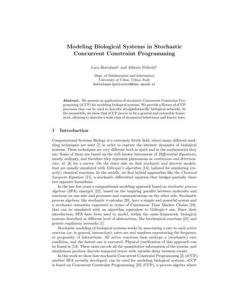
(IR1) 〈tell∞(c).A, d〉 −→ 〈A, d t c〉

(IR2) 〈p(x), d〉 −→ 〈A[x/y], d〉 if p(y) : −A

(IR3) 〈∃xA, d〉 −→ 〈A[y/x], d〉 with y fresh

(IR4)〈A1, d〉 −→ 〈A′1, d′〉

〈A1 ‖ A2, d〉 −→ 〈A′1 ‖ A2, d′〉

Table 2. Instantaneous transition for stochastic CCP

hand, are defined by the grammar in the last three lines of Table 1. There are twodifferent actions with temporal duration, i.e. ask and tell, identified by π. Theirrate λ is a function as specified above. These actions can be combined together intoa guarded choice M (actually, a mixed choice, as we allow both ask and tell to becombined with summation). In the definition of such choice, we force procedure callsto be always guarded. In fact, they are instantaneous operations, thus guarding them bya timed action allows to avoid instantaneous infinite recursive loops, like those possiblein p : −A ‖ p. In summary, an agent A can choose between different actions (M), itcan perform an instantaneous tell, it can declare a variable local (∃xA) or it can becombined in parallel with other agents.

The syntax presented here is slightly different from that of [2]. In fact, the classof instantaneous actions is expanded: in [2] it contained only the declaration of localvariables, while here it contains also procedure call and a version of tell. Nevertheless,the congruence relation defined in [2], ascribing the usual properties to the operatorsof the language (e.g. associativity and commutativity to + and ‖), remains the same.The configurations of sCCP programs will vary in the quotient space modulo thiscongruence relation, denoted by P.

2.3 Operational Semantics of sCCP

The definition of the operational semantics is given specifying two different kinds oftransitions: one dealing with instantaneous actions and the other with stochasticallytimed ones. This is also a novelty w.r.t. [2], though in the previous version an instanta-neous transition was implicitly defined in order to deal with local variables. The basicidea of this operational semantics is to apply the two transitions in an interleaved way:first we apply the transitive closure of the instantaneous transition, then we do onestep of the timed stochastic transition. To identify a state of the system, we need totake into account both the agents that are to be executed and the current configurationof the store. Therefore, a configuration will be a point in the space P × C.

The recursive definition of the instantaneous transition −→⊆ (P × C)× (P × C) isshown in Table 2. Rule (IR1) models the addition of a constraint in the store throughthe least upper bound operation of the lattice. Recursion corresponds to rule (IR2),which consists in substituting the actual variables to the formal parameters in the

(SR1) 〈tellλ(c).A, d〉 =⇒(1,λ(d))−−−−−−→〈A, d t c〉

(SR2) 〈askλ(c).A, d〉 =⇒(1,λ(d))−−−→〈A, d〉 if d ` c

(SR3)〈M1, d〉 =⇒(p,λ)

−−−−−→A′1, d

′�

〈M1 + M2, d〉 =⇒(p′,λ′)−−−−−→A′1, d

′�with p′ = pλ

λ+rate(M2,d)and λ′ = λ + rate(M2, d)

(SR4)〈A1, d〉 =⇒(p,λ)

−−−−−→A′1, d

′�

〈A1 ‖ A2, d〉 =⇒(p′,λ′)−−−−−−−−−→A′1 ‖ A2, d

′�with p′ = pλ

λ+rate(A2,d)and λ′ = λ + rate(A2, d)

Table 3. Stochastic transition relation for stochastic CCP

definition of the procedure called. In rule (IR3), local variables are replaced by freshglobal variables, while in (IR4) the other rules are extended compositionally. Observethat we do not need to deal with summation operator at the level of instantaneoustransition, as all the choices are guarded by (stochastically) timed actions. The syntacticrestrictions imposed to instantaneous actions guarantee that −→ can be applied onlyfor a finite number of steps. Moreover it can be proven that it is confluent. Given aconfiguration 〈A, d〉 of the system, we denote by

−−−→〈A, d〉 the configuration obtained byapplying the transitions −→ as long as it is possible (i.e., by applying the transitiveclosure of −→). The confluence property of −→ implies that

−−−→〈A, d〉 is well defined.The stochastic transition =⇒⊆ (P ×C)× [0, 1]×R+× (P ×C) is defined in Table 3.

This transition is labeled by two numbers: intuitively, the first one is the probabilityof the transition, while the second one is its global rate, see Section 2.4 for furtherdetails. Rule (SR1) deals with timed tell action, and works similarly to rule (IR1).Rule (SR2), instead, defines the behaviour of the ask instruction: it is active only ifthe asked constraint is entailed by the current configuration of the constraint store.Rules (SR3) and (SR4), finally, deal with the choice and the parallel construct. Notethat, after performing one step of the transition =⇒, we apply the transitive closure of−→. This guarantees that all actions enabled after one =⇒ step are timed. In Table 3we use the function rate : P × C → R, assigning to each agent its global rate. It isdefined as follows:

Definition 1. The function rate : P × C → R is defined by

1. rate (0, d) = 0;2. rate (tellλ(c).A, d) = λ(d);3. rate (askλ(c).A, d) = λ(d) if d ` c;4. rate (askλ(c).A, d) = 0 if d 6` c;5. rate (M1 + M2, d) = rate (M1, d) + rate (M2, d).6. rate (A1 ‖ A2, d) = rate (A1, d) + rate (A2, d);

Using relation =⇒, we can build a labeled transition system, whose nodes areconfigurations of the system and whose labeled edges correspond to derivable steps

of =⇒. As a matter of fact, this is a multi-graph, as we can derive more than onetransition connecting two nodes (consider the case of tellλ(c) + tellλ(c)). Starting fromthis labeled graph, we can build a Continuous Time Markov Chain (cf. [19] and nextsection) as follows: substitute each label (p, λ) with the real number pλ and add up thenumbers labeling edges connecting the same nodes. More details about the operationalsemantics can be found in [2].

2.4 Continuous Time Markov Chains and Gillespie’s Algorithm

A Continuous Time Markov Chain (CTMC for short) is a continuous-time stochasticprocess (Xt)t≥0 taking values in a discrete set of states S and satisfying the memorylessproperty, ∀n, t1, . . . , tn, s1, . . . , sn:

P{Xtn = sn | Xtn−1 = sn−1, . . . , Xt1 = s1} = P{Xtn = sn | Xtn−1 = sn−1}. (2.2)

A CTMC can be represented as a directed graph whose nodes correspond to the statesof S and whose edges are labeled by real numbers, which are the rates of exponentiallydistributed random variables (defined by the probability density (2.1)). In each statethere are usually several exiting edges, competing in a race condition in such a waythat the fastest one is executed. The time employed by each transition is drawn fromthe random variable associated to it. When the system changes state, it forgets its pastactivity and starts a new race condition (this is the memoryless property). Therefore,the traces of a CTMC are made by a sequence of states interleaved by variable timedelays, needed to move from one state to another.

The time evolution of a CTMC can be characterized equivalently by computing, ineach state, the normalized rates of the exit transitions and their sum (called the exitrate). The next state is chosen according to the probability distribution defined by thenormalized rates, while the time spent for the transition is drawn from an exponentiallydistributed random variable with parameter equal to the exit rate.

This second characterization can be used in a Monte-Carlo simulation algorithm.Suppose to be in state s; then draw two random numbers, one according to the proba-bility given by the normalized rates, and the second according to an exponential prob-ability distribution with parameter equal to the exit rate. Then choose the next stateaccording to the first random number, and increase the time according to the second.The procedure sketched here is essentially the content of the Gillespie’s algorithm [13,14], originally derived in the context of stochastic simulation of chemical reactions.Indeed, the stochastic description of chemical reactions is exactly a Continuous TimeMarkov Chain [12].

2.5 Stream Variables

In the use of sCCP as a modeling language for biological systems, many variables willrepresent quantities that vary over time, like the number of molecules of certain chem-ical species. In addition, the functions returning the stochastic rate of communicationswill depend only on those variables. Unfortunately, the variables we have at our dis-posal in CCP are rigid, in the sense that, whenever they are instantiated, they keepthat value forever. However, time-varying variables can be easily modeled as growinglists with an unbounded tail: X = [a1, . . . , an|T ]. When the quantity changes, we sim-ply need to add the new value, say b, at the end of the list by replacing the old tail

variable with a list containing b and a new tail variable: T = [b|T ′]. When we needto compute a function depending on the current value of the variable X, we need toextract from the list the value immediately preceding the unbounded tail. This can bedone by defining the appropriate predicates in the first-order language over which theconstraint store is built. As these variables have a special status in the presentationhereafter, we will refer to them as stream variables. In addition, we will use a simplifiednotation that hides all the details related to the list update. For instance, if we want toadd 1 to the current value of the stream variable X, we will simply write X = X + 1.The intended meaning of this notation is clearly: “extract the last ground element nin the list X, consider its successor n + 1 and add it to the list (instantiating the oldtail variable as a list containing the new ground element and a new tail variable)”.

2.6 Implementation

We have developed an interpreter for the language that can be used for running simula-tions. The simulation engine is based on the Gillespie’s Algorithm, therefore it performsa Monte-Carlo simulation of the underlying CTMC. The memoryless property of theCTMC guarantees that we do need to generate all its nodes to perform a simulation,but we need to store only the current state. By syntactic analysis of the current set ofagents in execution, we can construct all the exit transitions and compute their rates,evaluating rate functions w.r.t. the current configuration of the store (actually, thosefunctions depend only on stream variables, thus their computation has two steps: ex-tract the current value of the variables and evaluate the function). Then we apply theGillespie’s procedure to determine the next state and the elapsed time, updating thesystem by modifying the current set of agents and the constraint store according tothe chosen transition.

The interpreter is written in SICStus Prolog [10]. It is composed by a parser, ac-cepting a program written in sCCP and converting it into an internal list-based repre-sentation. The main engine operates therefore by inspecting and manipulating the listsrepresenting the program. The constraint store is managed using the constraint solveron finite domains of SICStus. Stream variables are not represented as lists, but ratheras global variables using the meta-predicates assert and retract of Prolog. The choiceof working with finite domains is mainly related to the fact that the biological systemsanalyzed can be described using only integer values1.

In every execution cycle we need to inspect all terms in order to check if theyenable a transition. Therefore, the complexity of each step is linear in the size of the(representation) of the program. This can be easily improved by observing that anenabled transition that is not executed remains enabled also in the future.

The correctness of the virtual machine can be proven by showing that it simulatesexactly the same CTMC defined by the sCCP program. This can be done by showingthat the exit rate and the probability distribution on exiting transitions are computedcorrectly, according to the operational semantics of sCCP.

Measurable Entities ↔ Stream Variables

Logical Entities ↔ Processes(Control Variables)

Interactions ↔ Processes

Table 4. Schema of the mapping between elements of biological systems (left) and sCCP(right).

3 Modeling Biological Systems

Taking an high level point of view, biological systems can be seen as composed essen-tially by two ingredients: (biological) entities and interactions among those entities.For instance, in biochemical reaction networks, the molecules are the entities and thechemical reactions are the possible interactions, see [22] and Section 3.1. In gene regu-latory networks, instead, the entities into play are genes and regulatory proteins, whilethe interactions are production and degradation of proteins, and repression and en-hancement of gene’s expression, cf. [1] and Section 3.2. In addition, entities fall intotwo separate classes: measurable and logical. Measurable entities are those present ina certain quantity in the system, like proteins or other molecules. Logical entities, in-stead, have a control function (like gene gates in [1]), hence they are neither producednor degraded. Note that logical entities are not real world entities, but rather they arepart of the models.

The translation scheme between the previously described elements and sCCP ob-jects is summarized in Table 4. Measurable entities are associated exactly to streamvariables introduced at the end of Section 2. Logical entities, instead, are representedas processes actively performing control activities. In addition, they can use variablesof the constraint store either as control variables or to exchange information. Finally,each interaction is associated to a process modifying the value of certain measurablestream variables of the system.

Associating variables to measurable entities means that we are representing themas part of the environment, while the active agents are associated to the differentactions capabilities of the system. These actions have a certain duration and a certainpropensity to happen: a fact represented here in the standard way, i.e. associating toeach action a stochastic rate. Actually, the speed of most of these actions dependson the quantity of the basic entities they act on. This fact shows clearly the need forhaving functional rates, which can be used to describe these dependencies explicitly.

In the next subsections we instantiate this general scheme, in order to deal with twoclasses of biological systems: networks of biochemical reactions and genetic regulatorynetworks.

1 The real valued rates and the stochastic evolution are tight with the definition of thesemantics and not with the syntax of the language, thus we do not need to represent themin the store.

3.1 Modeling Biochemical Reactions

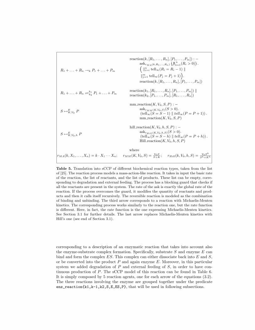
Network of biochemical reactions are usually modeled through chemical equations ofthe form R1 + . . . + Rn →k P1 + . . . + Pm, where the n reactants Ri’s (possibly inmultiple copies) are transformed into the m products Pj ’s. In the equation above,either n or m can be equal to zero; the case m = 0 represents a degradation reaction,while the case n = 0 represents an external feeding of the products, performed by anexperimenter. Actually, the latter is not a proper chemical reaction but rather a featureof the environmental setting, though it is convenient to represent it within the samescheme. Each reaction has an associated rate k, representing essentially its basic speed.The actual rate of the reaction is k · [R1] · · · [Rn], where [Ri] denotes the number ofmolecules Ri present in the system. There are cases when a more complex expressionfor the rate of the reaction is needed, see [25] for further details. For instance, onemay wish to describe an enzymatic reaction using a Michaelis-Menten kinetic law [8],rather than modeling explicitly the enzyme-substrate complex formation (as simpleinteraction/communication among molecules, cf. example below). A set of differentbiochemical arrows (corresponding to different biochemical laws) is shown in Table 5;this list is not exhaustive, but rather a subset of the one presented in [25]. Addingfurther arrows is almost always straightforward.

In Table 5, we also show how to translate biochemical reactions into sCCP processes.The basic reaction R1 + . . . + Rn →k P1 + . . . Pm is associated to a process that firstchecks if all the reactants needed are present in the system (asking if all [Ri] aregreater than zero), then it modifies the variables associated to reactants and products,and finally it calls itself recursively. Note that all the tell instructions have infiniterate, hence they are instantaneous transitions. The rate governing the speed of thereaction is the one associated to ask instruction. This rate is nothing but the functionrMA(k, X1, . . . , Xn) = k · X1 · · ·Xn representing mass action dynamics. Note that is a shorthand for the forward and the backward reactions. The arrow 7→E

K,V0has a

different dynamics, namely Michaelis-Menten kinetics: rMM (K, V0, S) = V0SS+K . This

reaction approximates the conversion of a substrate into a product due to the catalyticaction of enzyme E when the substrate is much more abundant than the enzyme (quasi-steady state assumption, cf. [8]). The last arrow, instead, is associated to Hill’s kinetics.The dynamics represented here is an improvement on the Michaelis-Menten law, wherethe exponent h encodes some information about the spatial behaviour of the reaction.

Comparing the encoding of biochemical reaction into sCCP with the encoding intoother process algebras like π-calculus [22], we note that the presence of functional ratesgives much more flexibility in the modeling phase. In fact, this form of rates allows todescribe dynamics that are different from Mass Action. Notable examples are exactlyMichaelis-Menten’s and Hill’s cases, represented by the last two arrows. This is notpossible wherever only constant rates are present, as the definition of the operationalsemantics constrain the dynamics to be Mass-Action like. More comments about thisfact can be found in [3].

Example: Enzymatic Reaction As a first and simple example, we show the modelof an enzymatic reaction. We provide two different descriptions, one using a mass actionkinetics, the other using a Michaelis-Menten one, see Table 5.

In the first case, we have the following set of reactions:

S + E k1k−1

ES →k2 P + E; P →kdeg; →kprod

S, (3.1)

R1 + . . . + Rn →k P1 + . . . + Pm

reaction(k, [R1, . . . , Rn], [P1, . . . , Pm]) : −askrMA(k,R1,...,Rn)

�Vni=1(Ri > 0)

�.�

‖ni=i tell∞(Ri = Ri − 1) ‖

‖mj=1 tell∞(Pj = Pj + 1)

�.

reaction(k, [R1, . . . , Rn], [P1, . . . , Pm])

R1 + . . . + Rn k1k2

P1 + . . . + Pmreaction(k1, [R1, . . . , Rn], [P1, . . . , Pm]) ‖reaction(k2, [P1, . . . , Pm], [R1, . . . , Rn])

S 7→EK,V0 P

mm reaction(K, V0, S, P ) : −askrMM (K,V0,S)(S > 0).(tell∞(S = S − 1) ‖ tell∞(P = P + 1)) .mm reaction(K, V0, S, P )

S 7→EK,V0,h P

hill reaction(K, V0, h, S, P ) : −askrHill(K,V0,h,S)(S > 0).(tell∞(S = S − h) ‖ tell∞(P = P + h)) .Hill reaction(K, V0, h, S, P )

where

rMA(k, X1, . . . , Xn) = k ·X1 · · ·Xn; rMM (K, V0, S) = V0SS+K

; rHill(k, V0, h, S) = V0Sh

Sh+Kh

Table 5. Translation into sCCP of different biochemical reaction types, taken from the listof [25]. The reaction process models a mass-action-like reaction. It takes in input the basic rateof the reaction, the list of reactants, and the list of products. These list can be empty, corre-sponding to degradation and external feeding. The process has a blocking guard that checks ifall the reactants are present in the system. The rate of the ask is exactly the global rate of thereaction. If the process overcomes the guard, it modifies the quantity of reactants and prod-ucts and then it calls itself recursively. The reversible reaction is modeled as the combinationof binding and unbinding. The third arrow corresponds to a reaction with Michaelis-Mentenkinetics. The corresponding process works similarly to the reaction one, but the rate functionis different. Here, in fact, the rate function is the one expressing Michaelis-Menten kinetics.See Section 3.1 for further details. The last arrow replaces Michaelis-Menten kinetics withHill’s one (see end of Section 3.1).

corresponding to a description of an enzymatic reaction that takes into account alsothe enzyme-substrate complex formation. Specifically, substrate S and enzyme E canbind and form the complex ES. This complex can either dissociate back into E and S,or be converted into the product P and again enzyme E. Moreover, in this particularsystem we added degradation of P and external feeding of S, in order to have con-tinuous production of P . The sCCP model of this reaction can be found in Table 6.It is simply composed by 5 reaction agents, one for each arrow of the equations (3.2).The three reactions involving the enzyme are grouped together under the predicateenz_reaction{k1,k-1,k2,S,E,ES,P}, that will be used in following subsections.

enz reaction(k1, k−1, k2, S, E, ES, P ) :-reaction(k1, [S, E], [ES]) ‖ reaction(k−1, [ES], [E, S]) ‖ reaction(k2, [ES], [E, P ]).

enz reaction(k1, k−1, k2, S, E, ES, P ) ‖ reaction(kprod, [], [S]) ‖ reaction(kdeg, [P ], [])

Table 6. sCCP program for an enzymatic reaction with mass action kinetics. The first blockdefines the predicate enz reaction(k1, k−1, k2, S, E, ES, P ), while the second block is the defi-nition of the entire program. The predicate reaction has been defined in Table 5.

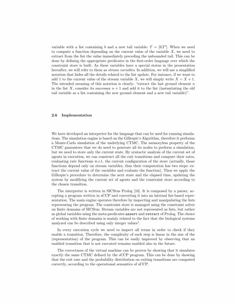
Simulations were performed with the simulator described in Section 2.6, and thetrend of product P is plotted in Figure 1 (left). Parameters of the system were chosenin order to have, at regime, almost all the enzyme molecules in the complexed state,see caption of Figure 1 (top) for details.

For this simple enzymatic reaction, the quasi-steady state assumption holds [8],therefore replacing the substrate-enzyme complex formation with a Michaelis-Mentenkinetics should leave the system behaviour unaltered. This intuition is confirmed byFigure 1 (bottom), showing the plot of the evolution over time of product P for thefollowing system of reactions:

S 7→EK,V0

P ; P →kdeg; →kprod

S,

whose sCCP can be derived easily from Table 5.A slightly more complicated version of the above example is the case in which some

level of cooperativity of the enzyme is to be modeled (Hill’s case). The set of reactionsin this case is an extension of the above one and can be written as:

n× S + E k1k−1

ESn →k2 n× P + E; P →kdeg; →kprod

S. (3.2)

In this case the sCCP program is a straightforward extension of the previous one:

n enz reaction(k1, k−1, k2, S, E, ES, P ) :-reaction(k1, [n× S, E], [ESn]) ‖ reaction(k−1, [ESn], [E, n× S]) ‖

reaction(k2, [ESn], [E, n× P ]).

while the rest of the coding is entirely similar to the previous case.Also in this case a comparison with the reaction obtained with the computed Hill

coefficientS 7→E

K,V0,n P ; P →kdeg; →kprod

S,

can be easily carried out. Notice that the Hill’s exponent corresponds exactly to thedegree of cooperativity of the enzyme.

Also a more refined approach to the case of Hill’s kinetics is possible, decomposingthe n-fold reaction in a series of n separated by Mass Action equation simulations.

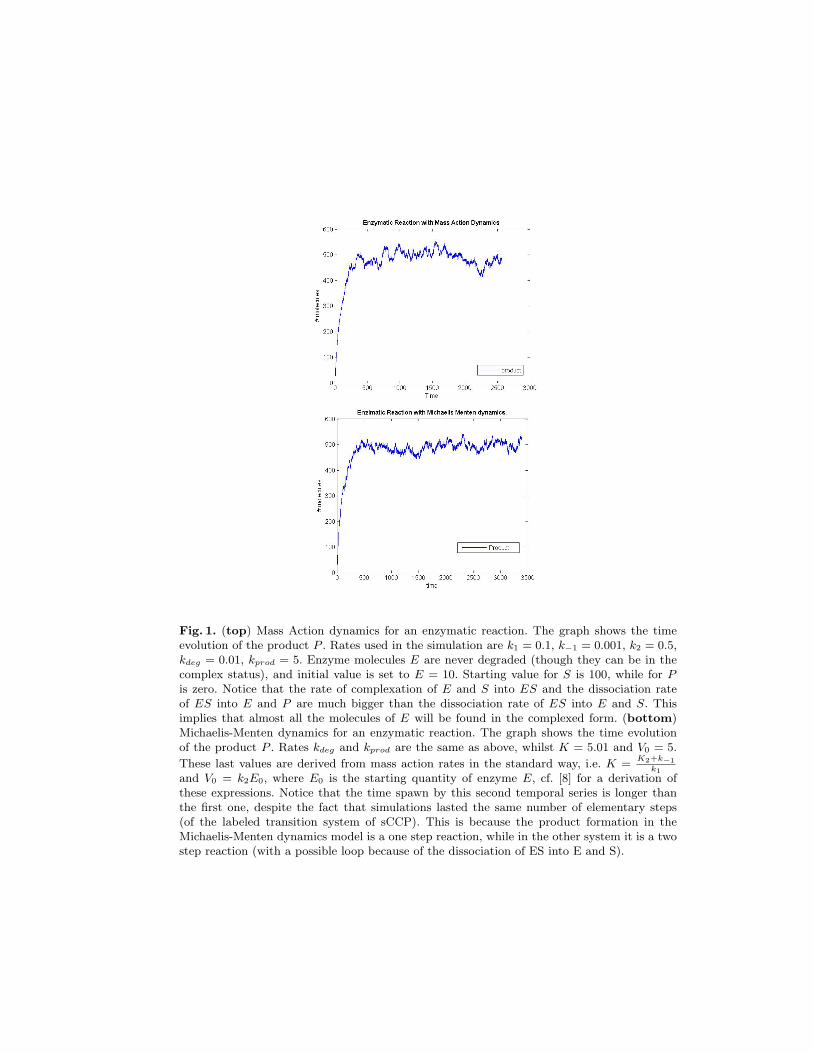
Fig. 1. (top) Mass Action dynamics for an enzymatic reaction. The graph shows the timeevolution of the product P . Rates used in the simulation are k1 = 0.1, k−1 = 0.001, k2 = 0.5,kdeg = 0.01, kprod = 5. Enzyme molecules E are never degraded (though they can be in thecomplex status), and initial value is set to E = 10. Starting value for S is 100, while for Pis zero. Notice that the rate of complexation of E and S into ES and the dissociation rateof ES into E and P are much bigger than the dissociation rate of ES into E and S. Thisimplies that almost all the molecules of E will be found in the complexed form. (bottom)Michaelis-Menten dynamics for an enzymatic reaction. The graph shows the time evolutionof the product P . Rates kdeg and kprod are the same as above, whilst K = 5.01 and V0 = 5.

These last values are derived from mass action rates in the standard way, i.e. K =K2+k−1

k1and V0 = k2E0, where E0 is the starting quantity of enzyme E, cf. [8] for a derivation ofthese expressions. Notice that the time spawn by this second temporal series is longer thanthe first one, despite the fact that simulations lasted the same number of elementary steps(of the labeled transition system of sCCP). This is because the product formation in theMichaelis-Menten dynamics model is a one step reaction, while in the other system it is a twostep reaction (with a possible loop because of the dissociation of ES into E and S).

enz reaction(ka, kd, kr, KKK, E1, KKKE1, KKKS) ‖enz reaction(ka, kd, kr, KKKS, E2, KKKSE2, KKK) ‖enz reaction(ka, kd, kr, KK, KKKS, KKKKKS, KKP ) ‖enz reaction(ka, kd, kr, KKP, KKP1, KKPKKP1, KK) ‖enz reaction(ka, kd, kr, KKP, KKKS, KKPKKKS, KKPP ) ‖enz reaction(ka, kd, kr, KKPP, KKP1, KKPPKKP1, KKP ) ‖enz reaction(ka, kd, kr, K, KKPP, KKKPP, KP ) ‖enz reaction(ka, kd, kr, KP, KP1, KPKP1, K) ‖enz reaction(ka, kd, kr, KP, KKPP, KPKKPP, KPP ) ‖enz reaction(ka, kd, kr, KPP, KP1, KPPKP1, KP )

Table 7. sCCP code for the MAP-Kinase signaling cascade. The enz reaction predicate hasbeen defined in Section 3.1. For this example, we set the complexation rates (ka), the dis-sociation rates (kd) and the product formation reaction rates (kr) equal for all the reactionsinvolved. For the actual values used in the simulation, refer to Figures 3 and 4.

Example: MAP-Kinase Cascade A cell is not an isolated system, but it communi-cates with the external environment using complex mechanisms. In particular, a cell isable to react to external signals, i.e. to signaling proteins (like hormones) present in theproximity of the external membrane. Roughly speaking, this membrane is filled withreceptor proteins, that have a part exposed toward the external environment capable ofbinding with the signaling protein. This binding modifies the structure of the receptorprotein, that can now trigger a chain of reactions inside the cell, transmitting the signalstraight to the nucleus. In this signaling cascade a predominant part is performed bya family of proteins, called Kinase, that have the capability of phosphorylating otherproteins. Phosphorylation is a modification of the protein fold by attaching a phos-phorus molecule to a particular amino acid of the protein. One interesting feature ofthese cascades of reactions is that they are activated only if the external stimulus isstrong enough. In addition, the activation of the protein at the end of the chain ofreactions (usually an enzyme involved in other regulation activities) is very quick. Thisbehaviour of the final enzyme goes under the name of ultra-sensitivity [17].

Fig. 2. Diagram of the MAP-Kinase cascade. The round-headed arrow schematically repre-sents an enzymatic reaction, see Section 3.1 for further details. This diagram has been stolenfrom a presentation of Luca Cardelli, held in Dobbiaco, September 2005.

In Figure 2 a particular signaling cascade is shown, involving MAP-Kinase pro-teins. This cascade has been analyzed using differential equations in [17] and thenmodeled and simulated in stochastic Pi-Calculus in [4] (CONTROLLARE SE E’ LACITAZIONE GIUSTA). We can see that the external stimulus, here generically rep-resented by the enzyme E1, triggers a chain of enzymatic reactions. MAPKKK isconverted into an active form, called MAPKKK*, that is capable of phosphorylatingthe protein MAPKK in two different sites. The diphosphorylated version MAPKK-PP of MAPKK is the enzyme stimulating the phosphorylation of another Kinase, i.e.MAPK. Finally, the diphosphorylated version MAPK-PP of MAPK is the output ofthe cascade.

The sCCP program describing MAP-Kinase cascade is shown in Table 7. The pro-gram itself is very simple, and it uses the mass action description of an enzymaticreaction (cf. Table 5). It basically consists in a list of the reactions involved, put inparallel. The real problem in studying such a system is in the determination of its 30parameters, corresponding to the basic rates of the reactions involved. In addition, weneed to fix a set of initial values for the proteins that respects their usual concentra-tions in the cell. Following [4], in Figure 3 we skip this problem and assign a value of1.0 to all basic rates, while putting 100 copies of MAPKKK, MAPKK and MAPK, 5copies of E2, MAPKK-P’ase, and MAPK-P’ase and just 1 copy of the input E1. Thissimple choice, however, is enough to predict correctly all the expected properties: theMAPK-PP time evolution, in fact, follows a sharp trend, jumping from zero to 100 ina short time. Remarkably, this property is not possessed by MAPKK-PP, the enzymein the middle of the cascade. Therefore, this switching behaviour exhibited by MAPK-PP is intrinsically connected with the double chain of phosphorylations, and cannotbe obtained by a simpler mechanism. Notice that the fact that the network works asexpected using an arbitrary set of rates is a good argument in favor of its robustnessand resistance to perturbations.

In Figure 4, instead, we choose a different set of parameters, as suggested in [17](cf. its caption). We also let the input strength vary, in order to see if the activationeffect is sensitive to its concentration. As we can see, this is the case: for a low valueof the input, no relevant quantity of MAPK-PP is present in the system.

3.2 Modeling Gene Regulatory Networks

In a cell, only a subset of genes are expressed at a certain time. Therefore, an importantmechanism of the cell is the regulation of gene expression. This is obtained by specificproteins, called transcription factors, that bind to the promoter region of genes (theportion of DNA preceding the coding region) in order to enhance or repress theirtranscription activity. These transcription factors are themselves produced by genes,thus the overall machinery is a networks of genes producing proteins that regulate othergenes. The resulting system is highly complex, containing several positive and negativefeedback loops, and usually very robust. This intrinsic complexity is a strong argumentin favor of the use of a mathematical formalism to describe and analyze them. In theliterature, different modeling techniques are used, see [7] for a Survey. However, wefocus on a modeling formalism based on stochastic π-calculus [1].

In [1], the authors propose to model gene networks using a small set of “logical”gates, called gene gates, encoding the possible regulatory activities that can be per-formed on a gene. Specifically, there are three types of gene gates: nullary gates, positive

Fig. 3. Temporal trace for some proteins involved in the MAP-Kinase cascade. Traces weregenerated simulating the sCCP program of Table 7. In this simulation, the rates ka, kd, kr

were all set to one. We can notice the sharp increase in the concentration of the outputenzyme, MAPK-PP, and its stability in the high expression level. The enzyme MAPKK-PP,the activator of MAPK phosphorylations, instead has a more unstable trend of expression.

gates and negative gates. Nullary gates represent genes with transcriptional activity, butwith no regulation. Positive gates are genes whose transcription rate can be increasedby a transcription factor. Finally, negative gates represent genes whose transcriptioncan be inhibited by the binding of a specific protein. At the level of abstraction of [1],the product of a gene gate is not a mRNA molecule, but directly the coded protein.These product proteins are then involved in the regulation activity of the same or ofother genes and can also be degraded.

We propose now an encoding of gene gates within sCCP framework, in the spirit ofTable 4. Proteins are measurable entities, thus they are encoded as stream variables;gene gates, instead, are logical control entities and they are encoded as agents. Thedegradation of proteins is modeled by the reaction agent of Table 5. In Table 8 wepresent the sCCP agents associated to gene gates. A nullary gate simply increases thequantity of the protein it produces at a certain specified rate. Positive gates, instead,can produce their coded protein at the basic rate or they can enter in an enhanced statewhere production happens at an higher rate. Entrance in this excited state happensat a rate proportional to the quantity of transcription factors present in the system.Negative gates behave similarly to positive ones, with the only difference that they canenter an inhibited state instead of an enhanced one. After some time, the inhibitedgate returns to its normal status. A specific gene, generally, can be regulated by morethan transcription factor. This can be obtained by composing in parallel the differentgene gates.

Example: Bistable Circuit The first example, taken from [1], is a gene networkcomposed by two negative gates repressing each other, see Figure 5. The sCCP modelfor this simple network comprehends two negative gates: the first producing protein Aand repressed by protein B, the second producing protein B and repressed by proteinA. In addition, there are the degradation reactions for proteins A and B. This network

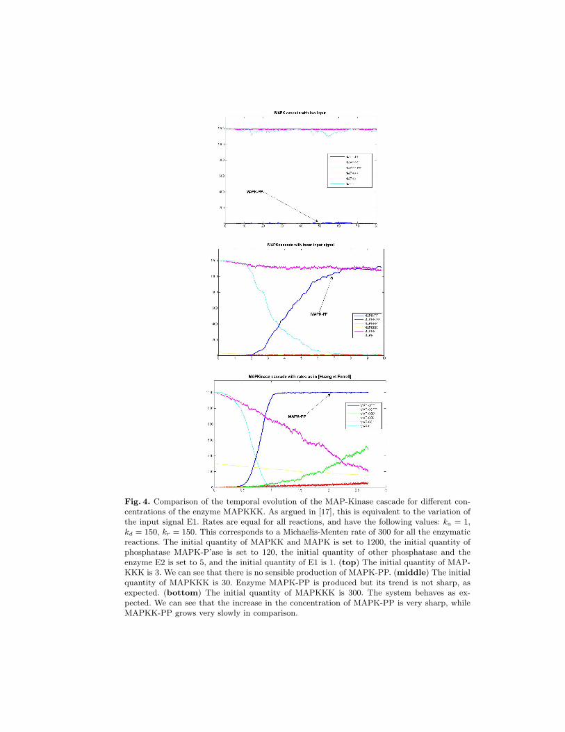
Fig. 4. Comparison of the temporal evolution of the MAP-Kinase cascade for different con-centrations of the enzyme MAPKKK. As argued in [17], this is equivalent to the variation ofthe input signal E1. Rates are equal for all reactions, and have the following values: ka = 1,kd = 150, kr = 150. This corresponds to a Michaelis-Menten rate of 300 for all the enzymaticreactions. The initial quantity of MAPKK and MAPK is set to 1200, the initial quantity ofphosphatase MAPK-P’ase is set to 120, the initial quantity of other phosphatase and theenzyme E2 is set to 5, and the initial quantity of E1 is 1. (top) The initial quantity of MAP-KKK is 3. We can see that there is no sensible production of MAPK-PP. (middle) The initialquantity of MAPKKK is 30. Enzyme MAPK-PP is produced but its trend is not sharp, asexpected. (bottom) The initial quantity of MAPKKK is 300. The system behaves as ex-pected. We can see that the increase in the concentration of MAPK-PP is very sharp, whileMAPKK-PP grows very slowly in comparison.

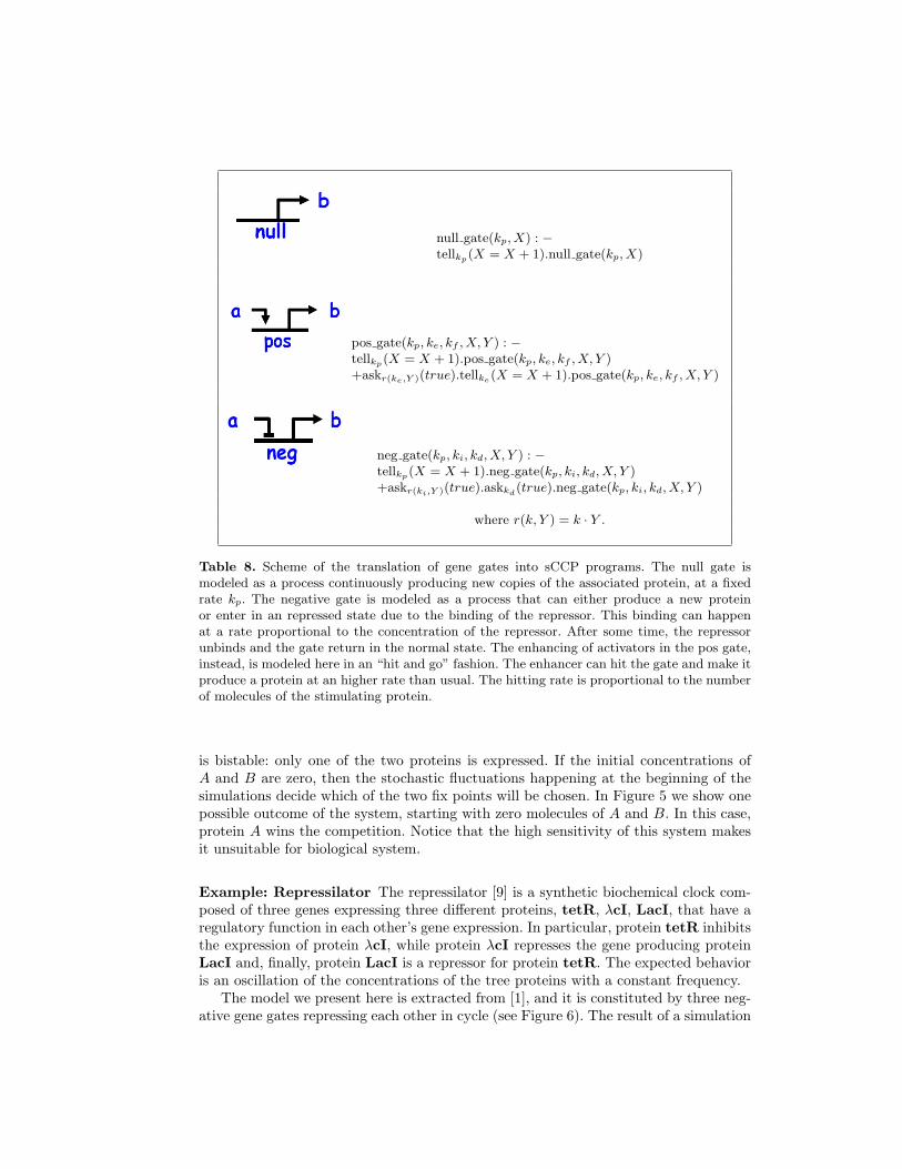
null gate(kp, X) : −tellkp(X = X + 1).null gate(kp, X)

pos gate(kp, ke, kf , X, Y ) : −tellkp(X = X + 1).pos gate(kp, ke, kf , X, Y )+askr(ke,Y )(true).tellke(X = X + 1).pos gate(kp, ke, kf , X, Y )

neg gate(kp, ki, kd, X, Y ) : −tellkp(X = X + 1).neg gate(kp, ki, kd, X, Y )+askr(ki,Y )(true).askkd(true).neg gate(kp, ki, kd, X, Y )

where r(k, Y ) = k · Y .

Table 8. Scheme of the translation of gene gates into sCCP programs. The null gate ismodeled as a process continuously producing new copies of the associated protein, at a fixedrate kp. The negative gate is modeled as a process that can either produce a new proteinor enter in an repressed state due to the binding of the repressor. This binding can happenat a rate proportional to the concentration of the repressor. After some time, the repressorunbinds and the gate return in the normal state. The enhancing of activators in the pos gate,instead, is modeled here in an “hit and go” fashion. The enhancer can hit the gate and make itproduce a protein at an higher rate than usual. The hitting rate is proportional to the numberof molecules of the stimulating protein.

is bistable: only one of the two proteins is expressed. If the initial concentrations ofA and B are zero, then the stochastic fluctuations happening at the beginning of thesimulations decide which of the two fix points will be chosen. In Figure 5 we show onepossible outcome of the system, starting with zero molecules of A and B. In this case,protein A wins the competition. Notice that the high sensitivity of this system makesit unsuitable for biological system.

Example: Repressilator The repressilator [9] is a synthetic biochemical clock com-posed of three genes expressing three different proteins, tetR, λcI, LacI, that have aregulatory function in each other’s gene expression. In particular, protein tetR inhibitsthe expression of protein λcI, while protein λcI represses the gene producing proteinLacI and, finally, protein LacI is a repressor for protein tetR. The expected behavioris an oscillation of the concentrations of the tree proteins with a constant frequency.

The model we present here is extracted from [1], and it is constituted by three neg-ative gene gates repressing each other in cycle (see Figure 6). The result of a simulation

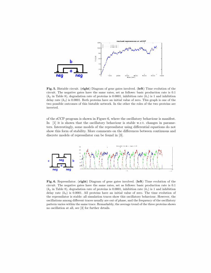
Fig. 5. Bistable circuit. (right) Diagram of gene gates involved. (left) Time evolution of thecircuit. The negative gates have the same rates, set as follows: basic production rate is 0.1(kp in Table 8), degradation rate of proteins is 0.0001, inhibition rate (ki) is 1 and inhibitiondelay rate (kd) is 0.0001. Both proteins have an initial value of zero. This graph is one of thetwo possible outcomes of this bistable network. In the other the roles of the two proteins areinverted.

of the sCCP program is shown in Figure 6, where the oscillatory behaviour is manifest.In [1] it is shown that the oscillatory behaviour is stable w.r.t. changes in parame-ters. Interestingly, some models of the repressilator using differential equations do notshow this form of stability. More comments on the differences between continuous anddiscrete models of repressilator can be found in [3].

Fig. 6. Repressilator. (right) Diagram of gene gates involved. (left) Time evolution of thecircuit. The negative gates have the same rates, set as follows: basic production rate is 0.1(kp in Table 8), degradation rate of proteins is 0.0001, inhibition rate (ki) is 1 and inhibitiondelay rate (kd) is 0.0001. All proteins have an initial value of zero. The time evolution ofthe repressilator is stable: all simulation traces show this oscillatory behaviour. However, theoscillations among different traces usually are out of phase, and the frequency of the oscillatorypattern varies within the same trace. Remarkably, the average trend of the three proteins showsno oscillation at all, see [3] for further details.

3.3 Modeling the Circadian Clock

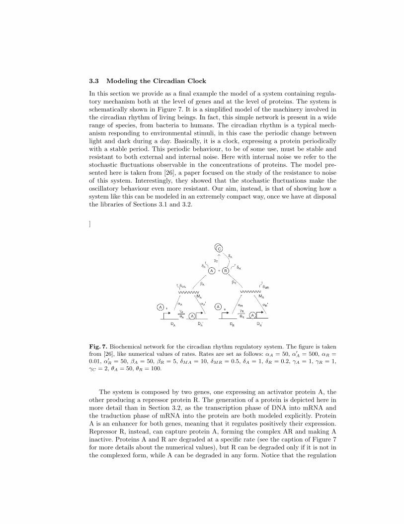
In this section we provide as a final example the model of a system containing regula-tory mechanism both at the level of genes and at the level of proteins. The system isschematically shown in Figure 7. It is a simplified model of the machinery involved inthe circadian rhythm of living beings. In fact, this simple network is present in a widerange of species, from bacteria to humans. The circadian rhythm is a typical mech-anism responding to environmental stimuli, in this case the periodic change betweenlight and dark during a day. Basically, it is a clock, expressing a protein periodicallywith a stable period. This periodic behaviour, to be of some use, must be stable andresistant to both external and internal noise. Here with internal noise we refer to thestochastic fluctuations observable in the concentrations of proteins. The model pre-sented here is taken from [26], a paper focused on the study of the resistance to noiseof this system. Interestingly, they showed that the stochastic fluctuations make theoscillatory behaviour even more resistant. Our aim, instead, is that of showing how asystem like this can be modeled in an extremely compact way, once we have at disposalthe libraries of Sections 3.1 and 3.2.

]

Fig. 7. Biochemical network for the circadian rhythm regulatory system. The figure is takenfrom [26], like numerical values of rates. Rates are set as follows: αA = 50, α′A = 500, αR =0.01, α′R = 50, βA = 50, βR = 5, δMA = 10, δMR = 0.5, δA = 1, δR = 0.2, γA = 1, γR = 1,γC = 2, θA = 50, θR = 100.

The system is composed by two genes, one expressing an activator protein A, theother producing a repressor protein R. The generation of a protein is depicted here inmore detail than in Section 3.2, as the transcription phase of DNA into mRNA andthe traduction phase of mRNA into the protein are both modeled explicitly. ProteinA is an enhancer for both genes, meaning that it regulates positively their expression.Repressor R, instead, can capture protein A, forming the complex AR and making Ainactive. Proteins A and R are degraded at a specific rate (see the caption of Figure 7for more details about the numerical values), but R can be degraded only if it is not inthe complexed form, while A can be degraded in any form. Notice that the regulation

pos gate(αA, α′A, γA, θA, MA, A) ‖pos gate(αR, α′R, γR, θR, MR, A) ‖

reaction(βA, [MA], [A]) ‖reaction(δMA, [MA], []) ‖reaction(βR, [MR], [R]) ‖reaction(δMR, [MR], []) ‖

reaction(γC , [A, R], [AR]) ‖reaction(δA, [AR], [R]) ‖

reaction(δA, [A], []) ‖reaction(δR, [R], [])

Table 9. sCCP program for the circadian rhythm regulation system of Figure 7. The agentsused have been defined in the previous sections. The first four reaction agents model the trans-lation of mRNA into the coded protein and its degradation. Then we have complex formation,and the degradation of R and A. The pos gate agent has been redefined as follows, in orderto take into account the binding/unbinding of the enhancer: pos gate(Kp, Ke, Kb, Ku, P, E):- pos gate off(Kp, Ke, Kb, Ku, P, E); pos gate off(Kp, Ke, Kb, Ku, P, E) :-tellKp(P = P + 1).pos gate off(Kp, Ke, Kb, Ku, P, E) + askrma(Kb,E)(E >0).pos gate on(Kp, Ke, Kb, Ku, P, E); pos gate on(Kp, Ke, Kb, Ku, P, E) :- tellKe(P =P + 1).pos gate on(Kp, Ke, Kb, Ku, P, E) + askKu(true).pos gate off(Kp, Ke, Kb, Ku, P, E).

activity of A is modeled by an explicit binding to the gene, which remains stimulateduntil A unbinds. This mechanism is slightly different from the positive gate describedin Section 3.2, but the code can be adapted in a straightforward manner (we simplyneed to define two states for the gene: bound and free, see caption of Table 9).

The code of the sCCP program modeling the system is shown in Table 9. It makesuse of the basic agents defined previously, and it is very compact and very easy andquick to write. In Figure 8 (top) we show the evolution of proteins A and R in a nu-merical simulation performed with the interpreter of the language. As we can see, theyoscillate periodically and the length of the period is remarkably stable. Figure 8 (bot-tom), instead, shows what happens if we replace the bind/unbind model of the genegate with the “hit and go” code of Section 3.2 (where the enhancer do not bind to thegene, but rather puts it into a stimulated state that makes the gene produce only thenext protein quicker). The result is dramatic, the periodic behaviour is lost and thesystem behaves in a chaotic way.

4 Conclusion and future work

In this paper we presented an application of stochastic concurrent constraint program-ming for modeling of biological systems. We dealt with two main classes of biologicalnetworks: biochemical reactions and gene regulation. The main theme is the use of con-straints in order to store information about the biological entities into play; this leadstraightforwardly to the definition of a general purpose library of processes that can beused in the modeling phase (see Sections 3.1 and 3.2). However, this is only a part ofthe general picture, as there are more complex classes of biological systems that need tobe modeled, like transport networks and membranes. In addition, all these systems are

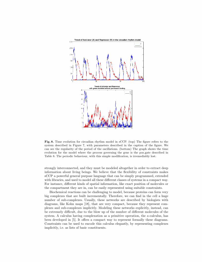
Fig. 8. Time evolution for circadian rhythm model in sCCP. (top) The figure refers to thesystem described in Figure 7, with parameters described in the caption of the figure. Wecan see the regularity of the period of the oscillations. (bottom) The graph shows the timeevolution for the model where the process governing the gene is the pos gate described inTable 8. The periodic behaviour, with this simple modification, is irremediably lost.

strongly interconnected, and they must be modeled altogether in order to extract deepinformation about living beings. We believe that the flexibility of constraints makessCCP a powerful general purpose language that can be simply programmed, extendedwith libraries, and used to model all these different classes of systems in a compact way.For instance, different kinds of spatial information, like exact position of molecules orthe compartment they are in, can be easily represented using suitable constraints.

Biochemical reactions can be challenging to model, because proteins can form verybig complexes that are built incrementally. Therefore, we can find in the cell a hugenumber of sub-complexes. Usually, these networks are described by biologists withdiagrams, like Kohn maps [18], that are very compact, because they represent com-plexes and sub-complexes implicitly. Modeling these networks explicitly, instead, canbe extremely difficult, due to the blow up of the number of different molecules of thesystem. A calculus having complexation as a primitive operation, the κ-calculus, hasbeen developed in [5]. It offers a compact way to represent formally these diagrams.Constraints can be used to encode this calculus elegantly, by representing complexesimplicitly, i.e. as lists of basic constituents.

Another interesting feature that sCCP offers are functional rates. As shown inSection 3.1, they can be used to represent more complex kinetic dynamics, allowing amore compact description of the networks. In this direction, we need to make deeperanalysis of the relation between these different kinetics in the context of stochasticsimulation, in order to characterize the cases where these different kinetics can be usedequivalently. Notice that the use of complex rates can be seen as an operation on theMarkov Chain, replacing a subgraph with a smaller one, hiding part of its complexity inthe expression of rates. This seems to be a sort of non-trivial lumpability relation [19],though further studies are necessary.

In [3], the authors investigate the expressivity gained by the addition of functionalrates to the language. They suggest that there is an increase of power in terms ofdynamical behaviours that can be reproduced, after encoding in sCCP a wide class ofdifferential equations. This problem, together with the inverse one of describing sCCPprograms by differential equations, is an interesting direction of research, which maylead to an integration of these different techniques, see [16, 3] for further comments.

Finally, we plan to implement a more powerful and fast interpreter for the lan-guage, using also all available tricks to increase the speed of stochastic simulations [12].Moreover, we plan to tackle also the problem of distributing efficiently the stochasticsimulations of programs written in sCCP.

References

1. R. Blossey, L. Cardelli, and A. Phillips. A compositional approach to the stochasticdynamics of gene networks. T. Comp. Sys. Biology, pages 99–122, 2006.

2. L. Bortolussi. Stochastic concurrent constraint programming. In Proceedings of 4th In-ternational Workshop on Quantitative Aspects of Programming Languages, QAPL 2006,2006.

3. L. Bortolussi and A. Policriti. Relating stochastic process algebras and differential equa-tions for biological modeling. Proceedings of PASTA 2006, 2006.

4. L. Cardelli and A. Phillips. A correct abstract machine for the stochastic pi-calculus. InProceeding of Bioconcur 2004, 2004.

5. V. Danos and C. Laneve. Formal molecular biology. Theor. Comput. Sci., 325(1):69–110,2004.

6. F.S. de Boer, A. Di Pierro, and C. Palamidessi. Nondeterminism and infinite computationsin constraint programming. Theoretical Computer Science, 151(1), 1995.

7. H. De Jong. Modeling and simulation of genetic regulatory systems: A literature review.Journal of Computational Biology, 9(1):67–103, 2002.

8. L. Edelstein-Keshet. Mathematical Models in Biology. SIAM, 2005.

9. M.B. Elowitz and S. Leibler. A syntetic oscillatory network of transcriptional regulators.Nature, 403:335–338, 2000.

10. Swedish Institute for Computer Science. Sicstus prolog home page.

11. D. Gillespie. The chemical langevin equation. Journal of Chemical Physics, 113(1):297–306, 2000.

12. D. Gillespie and L. Petzold. System Modelling in Cellular Biology, chapter NumericalSimulation for Biochemical Kinetics. MIT Press, 2006.

13. D.T. Gillespie. A general method for numerically simulating the stochastic time evolutionof coupled chemical reactions. J. of Computational Physics, 22, 1976.

14. D.T. Gillespie. Exact stochastic simulation of coupled chemical reactions. J. of PhysicalChemistry, 81(25), 1977.

15. L. Henkin, J.D. Monk, and A. Tarski. Cylindric Algebras, Part I. North-Holland, Ams-terdam, 1971.

16. J. Hillston. Fluid flow approximation of pepa models. In Proceedings of the SecondInternational Conference on the Quantitative Evaluation of Systems (QEST05), 2005.

17. C.F. Huang and J.T. Ferrell. Ultrasensitivity in the mitogen-activated protein kinasecascade. PNAS, Biochemistry, 151:10078–10083, 1996.

18. K. W. Kohn. Molecular interaction map of the mammalian cell cycle control and dnarepair systems. Molecular Biology of the Cell, 10:2703–2734, August 1999.

19. J. R. Norris. Markov Chains. Cambridge University Press, 1997.20. C. Priami. Stochastic π-calculus. The Computer Journal, 38(6):578–589, 1995.21. C. Priami and P. Quaglia. Stochastic π-calculus. Briefings in Bioinformatics, 5(3):259–

269, 2004.22. C. Priami, A. Regev, E. Y. Shapiro, and W. Silverman. Application of a stochastic name-

passing calculus to representation and simulation of molecular processes. Inf. Process.Lett., 80(1):25–31, 2001.

23. V. A. Saraswat. Concurrent Constraint Programming. MIT press, 1993.24. V. A. Saraswat, M. Rinard, and P. Panangaden. Semantics foundations of concurrent

constraint programming. In Proceedings of POPL, 1991.25. B. E. Shapiro, A. Levchenko, E. M. Meyerowitz, Wold B. J., and E. D. Mjolsness. Celler-

ator: extending a computer algebra system to include biochemical arrows for signal trans-duction simulations. Bioinformatics, 19(5):677–678, 2003.

26. J. M. G. Vilar, H. Yuan Kueh, N. Barkai, and S. Leibler. Mechanisms of noise resistancein genetic oscillators. PNAS, 99(9):5991, 2002.