Embed Size (px)
Citation preview

Modeling and statistical analysis of biomass productivity inphotobioreactors: Algafarm case study
Susana Alexandra dos Anjos Martins
Thesis to obtain the Master of Science Degree in
Chemical Engineering
Supervisor(s): Ana Paula Dias (IST)Joana Laranjeira (Allmicroalgae)
Examination Committee
Chairperson: Henrique Aníbal Santos de MatosSupervisor: Ana Paula Vieira Soares Pereira Dias
Member of the Committee: Ana Filipa da Silva Ferreira
November 2019

ii

Dedicated to someone special...
iii

iv

Acknowledgments
A todo este grande desafio com microalgas, farei alguns agradecimentos.
Em primeiro lugar, quero agradecer a Prof. Ana Paula Dias e a Dra. Joana Laranjeira pela oportu-
nidade de participar neste enorme desafio e de terem aceite orientar a minha dissertacao. A Prof. Ana
Paula Dias agradeco a disponibilidade e enorme interesse em ajudar no que fosse preciso na minha
tese, embora longe. A Dra Joana Laranjeira agradeco a confianca e liberdade de trabalho que deu aos
longos destes meses.
Agradeco a Ana Barros por me ter ajudado nos pontos chave e objetivos da tese, e por responder
sempre as minhas perguntas .
Um enorme obrigada tambem a Margarida que, desde a sua chegada, me tem apoiado e ajudado
em ınumeras situacoes da minha tese.
Ao Aldo, um grande obrigada por tudo o que me ensinou sobre estatıstica, todas as bases que me
deu sobre o modelo e por toda a disponibilidade em ajudar-me no que fosse preciso.
Agradeco tambem a todos os trabalhadores da Algafarm, principalmente ao pessoal dos laboratorios
que tanto chateei e a malta do UID. A Ines, Joana, Francisco, Pedro, Rosangela e Sara agradeco todos
os momentos passados nesta etapa e todo o companheirismo e amizade durante estes meses.
Aos meus grandes colegas de curso, Susana, Diogo Reis, Fitas e Cuco, um grande obrigada pela
aprendizagem, diversao, por tudo e mais alguma coisa que vivemos durante estes anos de curso.
Por ultimo, mas nao menos importante, um obrigada a minha famılia por sempre me ter apoiado e
encorajado nas mais diversas situacoes.
v

vi

Resumo
Um cultivo sequencial industrial na Allmicroalgae foi desenvolvido para a producao de elevada qual-
idade de biomassa de Chlorella vulgaris. Este processo comeca com o crescimento de celulas het-
erotroficas, em fermentadores, usados para alimentar diretamente fotobiorreactores (FBRs) no exterior.
A producao de biomassa nos FBRs depende de varios fatores, como a concentracao de amonia e taxa
final de crescimento da cultura no fermentador; concentracao inicial, temperatura, radiacao, tempo de
producao e area fotossintetica dos FBRs. Neste contexto, este trabalho teve como objetivo analisar e
integrar os dados, utilizando modelos estatısticos para prever as produtividades. Os dados foram anal-
isados no software R. A Analise de Componentes Principais detetou os fatores influencieveis na protu-
vidade . Modelos de regressao linear foram construıdos para prever a produtividade da biomassa em
funcao destes fatores. O metodo dos Mınimos Quadrados Ordinarios (MQO) foi aplicado nos sistemas
de inoculacao e dos Mınimos Quadrados Generalizado foi implementado em re-inoculacoes nos FBRs
devido a heterocedasticidade no metodo MQO. Estes modelos sublinharam a predominancia positiva
da temperatura e taxa final de crescimento para os sistemas de inoculacao e uma predominancia nega-
tiva da temperatura e do peso seco inicial para os sistemas de re-inoculacao. Os resultados mostraram
que a precisao dos modelos foi de 75% e 59% para os sistemas de inoculacao e re-inoculacao, respec-
tivamente. A inoculacao teve um desempenho melhor na previsao da produtividade da biomassa do
que nos sistemas de re-inoculacao. Estas conclusoes irao desenvolver estrategias de pre-tratamento
de dados para melhorar a producao de microalgas em FBRs.
Palavras-chave: Chlorella Vulgaris, fotobiorreatores, regressao linear multipla, analise de
componentes principais.
vii

viii
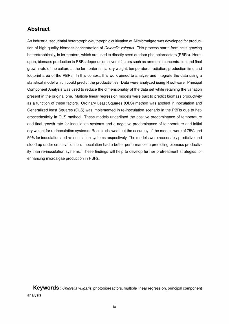
Abstract
An industrial sequential heterotrophic/autotrophic cultivation at Allmicroalgae was developed for produc-
tion of high quality biomass concentration of Chlorella vulgaris. This process starts from cells growing
heterotrophically, in fermenters, which are used to directly seed outdoor photobioreactors (PBRs). Here-
upon, biomass production in PBRs depends on several factors such as ammonia concentration and final
growth rate of the culture at the fermenter; initial dry weight, temperature, radiation, production time and
footprint area of the PBRs. In this context, this work aimed to analyze and integrate the data using a
statistical model which could predict the productivities. Data were analyzed using R software. Principal
Component Analysis was used to reduce the dimensionality of the data set while retaining the variation
present in the original one. Multiple linear regression models were built to predict biomass productivity
as a function of these factors. Ordinary Least Squares (OLS) method was applied in inoculation and
Generalized least Squares (GLS) was implemented in re-inoculation scenario in the PBRs due to het-
eroscedasticity in OLS method. These models underlined the positive predominance of temperature
and final growth rate for inoculation systems and a negative predominance of temperature and initial
dry weight for re-inoculation systems. Results showed that the accuracy of the models were of 75% and
59% for inoculation and re-inoculation systems respectively. The models were reasonably predictive and
stood up under cross-validation. Inoculation had a better performance in predicting biomass productiv-
ity than re-inoculation systems. These findings will help to develop further pretreatment strategies for
enhancing microalgae production in PBRs.
Keywords: Chlorella vulgaris, photobioreactors, multiple linear regression, principal component
analysis
ix

x

Contents
Acknowledgments . . . . . . . . . . . . . . . . . . . . . . . . . . . . . . . . . . . . . . . . . . . v
Resumo . . . . . . . . . . . . . . . . . . . . . . . . . . . . . . . . . . . . . . . . . . . . . . . . . vii
Abstract . . . . . . . . . . . . . . . . . . . . . . . . . . . . . . . . . . . . . . . . . . . . . . . . . ix
List of Tables . . . . . . . . . . . . . . . . . . . . . . . . . . . . . . . . . . . . . . . . . . . . . . xiii
List of Figures . . . . . . . . . . . . . . . . . . . . . . . . . . . . . . . . . . . . . . . . . . . . . xv
Nomenclature . . . . . . . . . . . . . . . . . . . . . . . . . . . . . . . . . . . . . . . . . . . . . . xix
Glossary . . . . . . . . . . . . . . . . . . . . . . . . . . . . . . . . . . . . . . . . . . . . . . . . 1
1 Introduction 1
1.1 Problem statement . . . . . . . . . . . . . . . . . . . . . . . . . . . . . . . . . . . . . . . . 1
1.2 Research Question . . . . . . . . . . . . . . . . . . . . . . . . . . . . . . . . . . . . . . . . 2
1.3 Outline of the thesis . . . . . . . . . . . . . . . . . . . . . . . . . . . . . . . . . . . . . . . 2
2 Literature review and background 3
2.1 Biological background . . . . . . . . . . . . . . . . . . . . . . . . . . . . . . . . . . . . . . 3
2.1.1 Microalgae overview . . . . . . . . . . . . . . . . . . . . . . . . . . . . . . . . . . 3
2.1.2 Growth dynamics . . . . . . . . . . . . . . . . . . . . . . . . . . . . . . . . . . . . . 3
2.1.3 Chlorella vulgaris . . . . . . . . . . . . . . . . . . . . . . . . . . . . . . . . . . . . . 4
2.1.4 Added-value compounds/ Biomass commercial value/Industrial applications . . . . 5
2.1.5 Industrial biomass cultivation . . . . . . . . . . . . . . . . . . . . . . . . . . . . . . 7
2.2 Statistical methods and data analysis . . . . . . . . . . . . . . . . . . . . . . . . . . . . . 10
2.2.1 Power of data analysis in biotechnology . . . . . . . . . . . . . . . . . . . . . . . . 10
2.2.2 Principal Component analysis . . . . . . . . . . . . . . . . . . . . . . . . . . . . . . 11
2.2.3 Regression analysis . . . . . . . . . . . . . . . . . . . . . . . . . . . . . . . . . . . 11
3 Materials and methods 21
3.1 General considerations . . . . . . . . . . . . . . . . . . . . . . . . . . . . . . . . . . . . . 21
3.2 Biological analysis . . . . . . . . . . . . . . . . . . . . . . . . . . . . . . . . . . . . . . . . 21
3.2.1 Optical density (OD) . . . . . . . . . . . . . . . . . . . . . . . . . . . . . . . . . . . 21
3.2.2 Dry weight . . . . . . . . . . . . . . . . . . . . . . . . . . . . . . . . . . . . . . . . 22
3.3 Chemical analysis . . . . . . . . . . . . . . . . . . . . . . . . . . . . . . . . . . . . . . . . 22
3.3.1 Ammonia concentration . . . . . . . . . . . . . . . . . . . . . . . . . . . . . . . . . 22
xi

3.4 Data analysis . . . . . . . . . . . . . . . . . . . . . . . . . . . . . . . . . . . . . . . . . . . 22
3.4.1 Software . . . . . . . . . . . . . . . . . . . . . . . . . . . . . . . . . . . . . . . . . 22
3.4.2 Statistical analysis . . . . . . . . . . . . . . . . . . . . . . . . . . . . . . . . . . . . 22
3.4.3 Regression analysis . . . . . . . . . . . . . . . . . . . . . . . . . . . . . . . . . . . 23
3.4.4 Variables . . . . . . . . . . . . . . . . . . . . . . . . . . . . . . . . . . . . . . . . . 23
4 Results and discussion 27
4.1 Principal component analysis . . . . . . . . . . . . . . . . . . . . . . . . . . . . . . . . . . 27
4.1.1 General PCA Classification Scheme . . . . . . . . . . . . . . . . . . . . . . . . . . 27
4.1.2 Inoculation systems . . . . . . . . . . . . . . . . . . . . . . . . . . . . . . . . . . . 27
4.1.3 Re-inoculation systems . . . . . . . . . . . . . . . . . . . . . . . . . . . . . . . . . 30
4.1.4 Comparing inoculation with re-inoculation systems . . . . . . . . . . . . . . . . . . 32
4.2 Regression- Construction of a predictive equation for inoculation and re-inoculation sys-
tem in photobioreactors . . . . . . . . . . . . . . . . . . . . . . . . . . . . . . . . . . . . . 33
4.2.1 General Regression Classification Scheme . . . . . . . . . . . . . . . . . . . . . . 33
4.2.2 Inoculation systems . . . . . . . . . . . . . . . . . . . . . . . . . . . . . . . . . . . 33
4.2.3 Re-inoculation systems . . . . . . . . . . . . . . . . . . . . . . . . . . . . . . . . . 39
4.2.4 Comparison of the performance of the predictive models . . . . . . . . . . . . . . . 45
5 Conclusions 49
5.1 Achievements . . . . . . . . . . . . . . . . . . . . . . . . . . . . . . . . . . . . . . . . . . . 49
5.2 Future Work . . . . . . . . . . . . . . . . . . . . . . . . . . . . . . . . . . . . . . . . . . . . 50
Bibliography 51
A Calibration Curve 61
A.1 Calibration Curve . . . . . . . . . . . . . . . . . . . . . . . . . . . . . . . . . . . . . . . . . 61
B Datasheets 63
B.1 Re-inoculation Datasheet . . . . . . . . . . . . . . . . . . . . . . . . . . . . . . . . . . . . 63
B.2 Inoculation Datasheet . . . . . . . . . . . . . . . . . . . . . . . . . . . . . . . . . . . . . . 64
B.3 Code for cross-validation . . . . . . . . . . . . . . . . . . . . . . . . . . . . . . . . . . . . 65
B.4 Results from MLR model . . . . . . . . . . . . . . . . . . . . . . . . . . . . . . . . . . . . 66
xii

List of Tables
2.1 Taxonomic classification of C. Vulgaris [20]. . . . . . . . . . . . . . . . . . . . . . . . . . . 5
2.2 Basic one-way ANOVA table. . . . . . . . . . . . . . . . . . . . . . . . . . . . . . . . . . . 14
4.1 Eigenvalues, percentage of variance and cumulative percentage of the correlation matrix
of the principal component analysis for inoculation systems. . . . . . . . . . . . . . . . . . 28
4.2 Eigenvalues, percentage of variance and cumulative percentage of the correlation matrix
of the principal component analysis for re-inoculation systems. . . . . . . . . . . . . . . . 30
4.3 Coefficient results and their respective statistic values ( standard error, p-value and t-
value) for the productivity model in inoculation systems. . . . . . . . . . . . . . . . . . . . 35
4.4 Coefficient results and their respective statistic values (standard error, p-value and t-
value) of the new model for productivity in inoculation systems. P-values from the co-
efficients have the higher levels of significance ***. . . . . . . . . . . . . . . . . . . . . . . 36
4.5 Residuals results for the productivity model in inoculation systems. . . . . . . . . . . . . . 36
4.6 ANOVA results for inoculation systems which productivity is the dependent variable. . . . 37
4.7 Coefficient results and their respective statistic values ( standard error, p-value and t-
value) for the productivity model in re-inoculation systems. . . . . . . . . . . . . . . . . . . 42
4.8 Coefficient results and their respective statistic values (standard error, p-value and t-
value) of the new model for productivity in re-inoculation systems. P-values from the
coefficients have the higher levels of significance ***. . . . . . . . . . . . . . . . . . . . . . 42
4.9 Residuals results of the model for productivity in re-inoculation systems. . . . . . . . . . . 42
4.10 Parameter estimates of GLS model for productivity in re-inoculation systems. . . . . . . . 44
4.11 Residuals results of the GLS model for productivity in re-inoculation systems. . . . . . . . 44
4.12 A comparison of the results of the productivity error of the predictive model for both inoc-
ulation systems. . . . . . . . . . . . . . . . . . . . . . . . . . . . . . . . . . . . . . . . . . 45
B.1 Re-inoculation data set from January 2019 until September 2019 . . . . . . . . . . . . . . 63
B.2 Inoculation data set from January 2018 until September 2019. . . . . . . . . . . . . . . . 64
xiii

xiv

List of Figures
1.1 Allmicroalgae’s production unit located in Pataias (Leiria) [1] . . . . . . . . . . . . . . . . . 1
2.1 Theoretical growth curve of microorganisms culture, highlighting: lag, exponential, de-
cline, stationary and dead phase. [16] . . . . . . . . . . . . . . . . . . . . . . . . . . . . . 4
2.2 Optical microscopic visualization of heterotrophic Chlorella vulgaris at Allmicroalgae, in
Zeiss Axio Scope A1 microscope with a 40x phase contrast. . . . . . . . . . . . . . . . . . 5
2.3 Pilot raceway open pound (a) and industrial photobioreactors (b) . . . . . . . . . . . . . . 7
2.4 Industrial fermenter with a volume of 5000 L installed in Allmicroalgae facilities. . . . . . 8
2.5 Scale-up growth of Chlorella vulgaris from the master cell bank up to a 5000 L fermenter.
This process can seed up to eight 100 m3 industrial photobioreactors (autotrophic route).
The culture volumes and the duration (days) of each scale-up step are indicated [60]. . . 9
2.6 Two five liters bench fermenters operating under the heterotrophic mode, at Allmicroalgae
facilities. . . . . . . . . . . . . . . . . . . . . . . . . . . . . . . . . . . . . . . . . . . . . . 9
2.7 Residuals vs fitted plots- the plot (a) presents a case of linearity and the plot (b) reveals a
non-linear relationship between variables [87]. . . . . . . . . . . . . . . . . . . . . . . . . 15
2.8 Example of quantile-quantile (QQ) plots. In case (a) residuals are normally distributed. In
case (b) non-normality is present [87]. . . . . . . . . . . . . . . . . . . . . . . . . . . . . . 16
2.9 General representation of scale location plots where in case (a) suggests constant vari-
ances in the residual and in case (b) is detected heteroscedasticity [87]. . . . . . . . . . . 16
2.10 Example of influential and not influential outliers. . . . . . . . . . . . . . . . . . . . . . . . 18
2.11 Plots of standardized residuals where in case (b) is detected one influential case [87]. . . 18
3.1 General engineering method to the model implementation for the problem under study. . . 21
3.2 Industrial contextualization of the selected variables for the model building. . . . . . . . . 25
4.1 Scree Plot of PCA eigenvalues for data analyzed in inoculation systems. . . . . . . . . . 28
4.2 Total contribution of variables to the first three principal components the generated PCA
for inoculation systems. The red dashed line on the graph indicates the average con-
tribution. The variable with a contribution above the line was considered relevant to the
components. . . . . . . . . . . . . . . . . . . . . . . . . . . . . . . . . . . . . . . . . . . . 29
xv

4.3 Principal component analysis of variables PC1 x PC2 for inoculation systems. Contrib
values are used to estimate the quality of the representation. Less influential variables
are blue colored. The most important ones are red colored. . . . . . . . . . . . . . . . . . 29
4.4 Scree Plot of PCA eigenvalues for data analyzed in re-inoculation systems. . . . . . . . . 31
4.5 Total contribution of variables to the first three principal components of the generated
PCA for re-inoculation systems. The red dashed line on the graph indicates the average
contribution. The variable with a contribution above the line was considered relevant to
the components. . . . . . . . . . . . . . . . . . . . . . . . . . . . . . . . . . . . . . . . . . 31
4.6 Principal component analysis of variables (PC1 x PC2) (a) and (PC2 x PC3) (b) for re-
inoculation systems. Contrib values are used to estimate the quality of the representation.
Less important variables are coloured by blue. The most important ones are coloured by
red. . . . . . . . . . . . . . . . . . . . . . . . . . . . . . . . . . . . . . . . . . . . . . . . . 32
4.7 Correlation matrix between the variables in inoculation systems. Positive correlations are
displayed in blue and negative correlations in red color. Color intensity is equivalent to the
correlation coefficients. Abbreviations meaning: temp- temperature, radi- radiation, fgrf-
final growth rate, idrw- initial dry weight, famc- ammonia concentration, prod- productivity 33
4.8 Scatter plot matrix that correlates all that variables present in the study. Abbreviations
meaning: Fgrf- final growth rate, Idrw- initial dry weight. . . . . . . . . . . . . . . . . . . . 34
4.9 Diagnostic Plots of Multiple Linear Regression Model for inoculation systems. . . . . . . . 38
4.10 Plots of the fitted model in terms how the variables final growth rate (a) and temperature
(b) were estimated to affect the productivity for inoculation systems. The blue line indi-
cates the expected value, the gray band a confidence interval for the expected value and
the dark gray dots the partial residuals. . . . . . . . . . . . . . . . . . . . . . . . . . . . . 39
4.11 Correlation matrix between the variables in re-inoculation systems. Abbreviations mean-
ing: temp- temperature, radi- radiation, fgrf- final growth rate, idrw- initial dry weight, famc-
ammonia concentration, prod- productivity. . . . . . . . . . . . . . . . . . . . . . . . . . . 40
4.12 Scatter plot matrix that correlates all that variables present in the study. Abbreviations
meaning: Fgrf- final growth rate, Idrw- initial dry weight. . . . . . . . . . . . . . . . . . . . 41
4.13 Diagnostic Plots of Multiple Linear Regression Model for re-inoculation systems. . . . . . 43
4.14 Plots of the fitted model in terms of how the variables Temperature (a) and Initial dry
weight (b) were estimated to affect the productivity for re-inoculation systems. The blue
line indicates the expected value and the dark gray dots the partial residuals. . . . . . . . 45
4.15 The performance result of productivity obtained from the models and from the real pro-
ductivity in the photobioreactors for each sample in inoculation (a) and re-inoculation (b)
systems. . . . . . . . . . . . . . . . . . . . . . . . . . . . . . . . . . . . . . . . . . . . . . . 46
A.1 Absorbance of Chlorella vulgaris measured at λ=600 nm versus biomass concentration
in autotrophic growth. . . . . . . . . . . . . . . . . . . . . . . . . . . . . . . . . . . . . . . 61
B.1 Code of the hold out validation method for the two inoculation systems. . . . . . . . . . . 65
xvi

B.2 Generalized least squares results for re-inoculation systems. . . . . . . . . . . . . . . . . 66
B.3 Ordinary least squares results for inoculation systems. . . . . . . . . . . . . . . . . . . . . 66
xvii

xviii

Nomenclature
Subscripts
AIC Akaike information criterion .
ANOVA Analysis of Variance .
BLUE Best linear unbiased estimate.
COD chemical oxygen demand .
CRAN Comprehensive R Archive Network .
df degrees of freedom .
DHA docosapanthenoic .
DW Dry weight.
EPA eicosapanthenoic acid .
GLS Generalized least squares.
MAE Mean absolute error.
MAPE Mean absolute percentage error.
MLR Multiple linear regression.
MSE Mean sum of squares due to error .
MSR Mean sum of squares due to regression .
MST Total mean sum of squares .
OD Optical density.
OLS Ordinary least squares.
PC Principal Component .
PCA Principal component analysis.
QQ Quantile-Quantile.
xix

RMSE Root mean square error.
RSE Residual Standard Error.
SE Standard Error.
SSE sum of squared errors.
SSE sum of squares due to error .
SSR sum of squared residuals .
SST total sum of squares .
VIF Variance inflation factor.
xx

Chapter 1
Introduction
1.1 Problem statement
The dissertation was carried out at Allmicroalgae, a microalgae production unit associated to the cement
company Cimentos Maceira e Pataias (CMP), SECIL Group, located in Pataias (Leiria).
Figure 1.1: Allmicroalgae’s production unit located in Pataias (Leiria) [1]
SECIL was founded in Portugal where it is the leading cement producer. This company also operates
internationally in Angola, Tunisia, Lebanon, Cape Verde, The Netherlands and Brazil (SECIL, 2018).
The cement industry is the third-largest source of anthropogenic carbon dioxide emissions to the
atmosphere. During clinker production, carbon dioxide is emitted as a by-product, in which calcium
carbonate (CaCO3) is decomposed into oxides (CaO), the primary component of cement. Thus, despite
its emission during cement production, CO2 is also emitted by fossil fuel combustion [2]. Total emissions
from the cement industry could contribute about 8 % of global CO2 emissions [3].
Allmicroalgae was developed by Secil with the perspective of using microalgae to sequester and cap-
ture the CO2 resulting from the cement production process. This unit is the largest industrial production
of microalgae in Europe [4]. The plant has a volume of autotrophic production higher than 1300 m3 [5].
Recently, a heterotrophic growth unit was developed, which bases the production in 200 and 5000 L fer-
1
menters. Currently, Chlorella vulgaris and Nannochloropsis oceanica are the main microalgae species
being produced in Algafarm for food and feed applications, respectively [1].
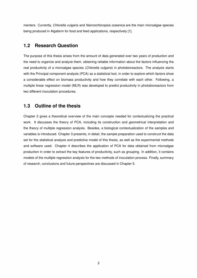
1.2 Research Question
The purpose of this thesis arises from the amount of data generated over two years of production and
the need to organize and analyze them, obtaining reliable information about the factors influencing the
real productivity of a microalgae species (Chlorella vulgaris) in photobioreactors. The analysis starts
with the Principal component analysis (PCA) as a statistical tool, in order to explore which factors show
a considerable effect on biomass productivity and how they correlate with each other. Following, a
multiple linear regression model (MLR) was developed to predict productivity in photobioreactors from
two different inoculation procedures.
1.3 Outline of the thesis
Chapter 2 gives a theoretical overview of the main concepts needed for contextualizing the practical
work. It discusses the theory of PCA, including its construction and geometrical interpretation and
the theory of multiple regression analysis. Besides, a biological contextualization of the samples and
variables is introduced. Chapter 3 presents, in detail, the sample preparation used to construct the data
set for the statistical analysis and predictive model of this thesis, as well as the experimental methods
and software used. Chapter 4 describes the application of PCA for data obtained from microalgae
production in order to extract the key features of productivity, such as grouping. In addition, it contains
models of the multiple regression analysis for the two methods of inoculation process. Finally, summary
of research, conclusions and future perspectives are discussed in Chapter 5.
2

Chapter 2
Literature review and background
2.1 Biological background
2.1.1 Microalgae overview
Microalgae are unicellular and photosynthetic microorganisms that include eukaryotes such as green,
red, brown and golden algae, diatoms, dinoflagellates, as well as prokaryotic cyanobacteria [6] [7].
They can grow rapidly in aquatic environments such as freshwater, wastewater, and the marine
environment [8], but they appear, as well, in terrestrial environments such as soil [9]. Once microalgae
grow 10–50 times faster than terrestrial plants [10], CO2 removal efficiency of microalgae is ten times
higher than that of terrestrial plants. Consequently they produce two- to tenfold more biomass per unit
land area than the best terrestrial systems [11].
Some species can tolerate the most extreme environments such as a wide range of temperatures,
salinities, and pHs; different light intensities; conditions in reservoirs or deserts, grow alone or in sym-
biosis with other organisms [12].
Microalgae are responsible for over 50% of the primary photosynthetic productivity on Earth and are
an essential link in the food chain. They also contribute 50 to 87% to global oxygen production [13].
Although there are differences in the composition between genera, species, and strains, protein is
the major organic constituent, followed by lipids and then by carbohydrates, according to the Food and
Agricultural Organisation (FAO). The reported levels of proteins, lipids, and carbohydrates are 12-35%,
7.2-23%, and 4.6-23%, respectively, expressed as percentage of dry weight [14]. Microalgae are the
primary producers of eicosapentaenoic acid (EPA) and docosahexaenoic acid (DHA) in the food chain
and provide also other high-value molecules (such as pigments and triacylglycerols) [15].
2.1.2 Growth dynamics
Life-cycle of microalgae cultures, as generally all microorganisms, is characterized by five different
phases, namely: lag, exponential, decline, stationary and dead phase. The variation in cell concen-
tration during the time is illustrated in figure 2.1. Each one of these five phases represents a distinct
3

period of growth that is associated with typical physiological and physicochemical changes in cell culture
[16].
Figure 2.1: Theoretical growth curve of microorganisms culture, highlighting: lag, exponential, decline,stationary and dead phase. [16]
After inoculation, cells use the lag phase to adapt to their new environment, keeping the same con-
centration. The inoculation process is usually followed by this phase. Microalgae have short lag phases
if cultures are inoculated with exponentially growing inocula [17]. The growth phase appears when the
cells have already adapted to themselves and to the environmental conditions. During this phase cul-
ture grows under no limitations in available nutrients or light. However, when growth rate reaches its
maximum, the culture stops growing. This occurs when nutrients, light, carbon dioxide or other factors
become inhibitory or theis culture medium depleted the growth slows down and the cells enter the de-
cline phase. After that, starts the stationary phase in which cell density become constant and the growth
rate ceases. Some cultures exhibit a death phase as cells lose viability or are destroyed by lysis. [16]
2.1.3 Chlorella vulgaris
Chlorella vulgaris is a green eukaryotic and unicellular microalgae with a spherical microscopic cell with
2–10 µm diameter [18] . A microscopic visualization can be seen in Figure 2.2. C. vulgaris has a thick
and rigid cell wall due to its hemicellulotic content [19] [18].
Chlorella vulgaris is a freshwater species of Chlorella that reproduces asexually and quickly by au-
tosporulation. Within 24 h, one cell of C. vulgaris growing in optimal conditions can multiply by au-
tosporulation. C. vulgaris taxonomical position is demonstrated in Table 2.1.
Total protein content in mature C.vulgaris represents 42–58 % of biomass dry weight [21] [22], de-
pending on growing/medium conditions. It synthesizes essential and non-essential amino acids, so it
is considered to have a high protein nutritional quality, according to the standard amino acid profile for
human nutrition proposed by the World Health Organisation (WHO) and the Food and Agricultural Or-
ganisation (FAO). C.vulgaris can reach 5–40% lipids per dry weight of biomass and those are mainly
4

Figure 2.2: Optical microscopic visualization of heterotrophic Chlorella vulgaris at Allmicroalgae, in ZeissAxio Scope A1 microscope with a 40x phase contrast.
Table 2.1: Taxonomic classification of C. Vulgaris [20].
Empire Eukaryota
Kingdom Plantae
Phylum Chlorophyta
Class Trebouxiophyceae
Order Chlorellales
Family Chlorellaceae
Genus Chlorella
composed by glycolipids, waxes, phospholipids, and small amounts of free fatty acids [21].
Regarding carbohydrates, starch is the most abundant polysaccharide in C.vulgaris [23]. Under
nitrogen limitation, a fast increase in carbohydrates is seen, reaching a total carbohydrates content of
13–55% dry weight [24] [25] [26].
Chlorophylls, specifically chlorophyll a and b, are the most abundant pigments in C.vulgaris, repre-
senting 1–2% of its dry weight [23]. Carotenoids are other important pigments known to have numerous
therapeutic qualities, such as: antioxidant properties, blood cholesterol regulation, enhancement of the
immune system. Total carotenoid content can reach 0.8% of biomass dry weight in Chlorella spp.,
depending on growth conditions [27].
2.1.4 Added-value compounds/ Biomass commercial value/Industrial applica-
tions
The industrial cultivation of microalgae aiming the production of biofuels and bioproducts has increased
dramatically over the last few decades [28].
The biggest field of application is the food sector. C. vulgaris and Spirulina platensis have been rec-
ognized by the US FDA (Food and Drug Administration) and by EFSA (European Food Safety Authority)
as safe to use as additives in food and beverages due to their protein content on a dry basis [29]. Several
species of microalgae produce high quantities of the essential amino acids, bioactive non-essential and
5

proteins, which can be used protection against many diseases [30]. The quantity of produced protein
can be compared to other rich sources of proteins, for example: egg, milk and meat. Some species of
microalgae produce 2.5–7.5 tons/ha/year of proteins [31].
Carotenoids produced by microalgae and other plants, mostly beta-carotene, are used for coloring
additive in food (E 160 IV) due to its coloring agent and pro-vitamin A in aquaculture and livestock feeds
[32] [33]. Another important carotenoid, obtained from Haematoccocus pluvialis, is astaxanthin. It is
incorporated into the diets of salmonoids, shrimp, and crayfish as a supplement of food colorant, pink
flesh [34]. From all carotenoids, lutein is the most abundant carotenoid in C.vulgaris [35].
Lipids produced by microalgae are also used in the food industry. Long-chain fatty acids in particular
omega-3, eicosapentaenoic acid (EPA), and docosapentaenoic acid (DHA) are the most requested lipids
to prevent cardiovascular disease [29]. The lipid content extracted from the species Ulkenia sp. and
Schizochytrium sp., is used to enrich omega-3 foods and drinks for lactating women and other adults
[29].
About 30% of microalgal production is sold for animal feed due to the growing demand for natural
composition instead of synthesized ingredients [19]. Aquaculture is the main sector for microalgae
once they represent a rich source of omega-3, proteins, vitamins and carotenoids [33]. For example,
Haematococcus pluvialis in the red phase is used as a coloring additive to feed shrimps and salmonids
both as dried biomass and as astaxanthin extracts [29].
Some microalgae species have high levels of sterols, namely phytosterols. They show beneficial
health effects such as hypo-cholesterolemia, anticancer, anti-inflammatory and a role in neurological
diseases like Parkinson’s disease [36] [37].
Also, the first reported antibacterial products in microalgae were in the green microalga Chlorella,
which significantly inhibits the growth of both Gram-positive and Gram-negative bacteria [38].
Due to climate change, deficiency of natural sources and the uprising energy crisis, microalgae has
earned interest as a biofuel feedstock to biorefineries [39]. Third-generation biofuel from microalgae is
considered as one of the alternatives to current biofuel crops such as soybean, corn, rapeseed, and
lignocellulosic feedstocks once it does not compete with food and does not require arable lands to grow.
However, biofuel from microalgae has high production costs and only for that reason cannot still compete
with conventional fuels [39].
Microalgae also have numerous applications in wastewater treatment. C.Vulgaris absorbs 45–97% of
nitrogen, 28–96% of phosphorus and in reducing the chemical oxygen demand (COD) by 61–86% from
different types of wastewater such as textiles, sewage, municipal, agricultural and recalcitrant [40] [41].
They promote the removal of vital nutrients (nitrogen and phosphorus), carbon dioxide, heavy metals and
pathogens present in wastewaters, necessary for their growth [42]. A faster growth rate accompanied
by an elimination of water-contamination level is a promising process. C. vulgaris promotes impressive
total removal ammonium and sometimes has potential to eliminate phosphorus present in the medium
[43].
Bio-fertilizers with microalgae extracts increase the growth parameters of many plants due to the rich
composition in macronutrients such as nitrogen, phosphorus and potassium. Microalgae also contain
6
plant growth-promoting substances such as carotenoids, vitamins, amino acids, and antifungal sub-
stances [44].
2.1.5 Industrial biomass cultivation
The three major cultivation modes in which microalgae can be produced are: photoautotrophic, het-
erotrophic, and mixotrophic cultivation.
Autotrophic cultivation of microalgae can be conducted in open ponds and closed reactors. In au-
totrophic processes there are requirements to be satisfied such as: the supply of light and nutrients
(mainly carbon, nitrogen, phosphorous), the control of adequate culture conditions (temperature and
pH) and mixing to avoid gradients of these parameters that reducing the productivity [45] [46].
Open systems, such as water tanks, natural ponds and raceway ponds are presently the most com-
mon operational technology for outdoor solar cultivation. Raceway ponds which is currently the most
used and cheapest cultivation system for production of microalgae, have a lower capital cost than a
photobioreactors, however they are more prone to contamination and water losses due to evaporation
[47]. In addition, the use of carbon sources is not optimal; therefore, some improvements need to be
done. Despite having a higher production cost, closed photobioreactors do not require such as huge
ground area compared to raceways ponds. Closed and controlled medium conditions make this system
less contaminable. There is a wide diversity of PBRs technologies such as tubular manifold, flat-plate,
vertical tubular serpentine and among others. Tubular PBRs are the most common design of closed
systems currently developed at industrial scale [48]. A PBR is a bioreactor that utilizes a light source to
cultivate phototrophic microorganisms, generating biomass from light and carbon dioxide [49].
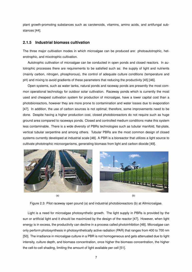
(a) (b)
Figure 2.3: Pilot raceway open pound (a) and industrial photobioreactors (b) at Allmicroalgae.
Light is a need for microalgae photosynthetic growth. The light supply in PBRs is provided by the
sun or artificial light and it should be maximized by the design of the reactor [47]. However, when light
energy is in excess, the productivity can decline in a process called photoinhibition [48]. Microalgae can
only perform photosynthesis in photosynthetically active radiation (PAR) that ranges from 400 to 700 nm
[50]. The irradiance in microalgae culture in a PBR is not homogeneous and gets attenuated due to light
intensity, culture depth, and biomass concentration, once higher the biomass concentration, the higher
the cell-to-cell shading, limiting the amount of light available per cell [51].
7

When the objective is to produce biomass in standard growth conditions, nutrients are provided in
excess in the culture medium. Nitrogen can be supplied as urea, nitrate, or ammonium. CO2 is the
carbon source and it has also to be in excess [47]. The CO2 transfer, its dissolution and consumption
results in pH modifications and therefore the pH is controlled by CO2 supply.
The temperature in microalgae cultures increases or decreases according to absorption of heat
by radiation from the light source. Growth of microalgae was stunted during prolonged periods of bad
weather such as cloudy or rainy days [52]. The light source is insufficient, causing a decrease in biomass
productivity and biochemical composition of microalgae cells [52]. The optimal temperature for most
microalgae growth ranges from 20 ◦C to 35 ◦C, although Chlorella vulgaris can tolerate up to 40 ◦C.
Overheating of the cultures can kill the cells and below the optimal temperature, the productivity of the
culture gets reduced [53]. The supply of heat by sun radiation in large-scale reactors operated outdoors
is high, so water spray is the method used to avoid overheating in outdoor systems [54].
In heterotrophic growth, cells do not require light and the carbon supply of autotrophic cultures is
replaced by organic carbon sources dissolved in the culture medium [55]. Hereupon, heterotrophy is
defined as the use of organic compounds for growth [56]. Microalgae cultured in Allmicroalgae under
heterotrophy grow in a stirred tank bioreactor, or fermenter, operated in fed-batch, as seen in Figure 2.4
Figure 2.4: Industrial fermenter with a volume of 5000 L installed in Allmicroalgae facilities.
The most commonly used carbon sources for C.vulgaris in heterotrophy are glucose, acetate, and
glycerol. Ammonium is the preferred nitrogen source once less energy is required for its uptake, com-
pared with other N-sources as urea, nitrate and others [56]. Ammonium concentration varies depending
on several factors, including the fluctuations [57].
High cell density and biomass productivity may be quickly obtained through this growth mode [58],
when compared to autotrophy. However, producing light-induced metabolites such as pigments is not
so effective.
Microalgae can also be grown in mixotrophic regime, which is a combination of both autotrophic and
heterotrophic techniques. Cultures perform photosynthesis and respiration metabolism concurrently
[8]. Mixotrophic cultivation utilizes both organic and inorganic carbon sources. Mixotrophic growth can
8

achieve higher growth rate and greater lipid content than photoautotrophy, however high cell density
cultures as the ones obtained in heterotrophy are not possible. Hence, concentration costs and the
susceptibility to stress become a very limited cultivation condition [59].
2.1.5.1 Microalgae biofactory -Allmicroalgae case study
Chlorella vulgaris can growth under sequential heterotrophic/ autotrophic conditions. It has the capability
to metabolically shift in response to changes in the environment and culture conditions [58].
To improve microalgal scale-up a two-stage production was implemented in Allmicroalgae, combining
of heterotrophic and autotrophic cultivation modes, as represented in Figure 2.5.
Figure 2.5: Scale-up growth of Chlorella vulgaris from the master cell bank up to a 5000 L fermenter.This process can seed up to eight 100 m3 industrial photobioreactors (autotrophic route). The culturevolumes and the duration (days) of each scale-up step are indicated [60].
The seed culture of C. vulgaris is obtained in 50 mL and 250 mL Erlenmeyer’s by heterotrophic
growth in order to reach a five liters fermenter, as seen in Figure 2.6 .
Figure 2.6: Two five liters bench fermenters operating under the heterotrophic mode, at Allmicroalgaefacilities.
The culture obtained by two of 5 L fermenters for 3 days cultivation will further inoculate the 5000 L
industrial fermenter. In the heterotrophic medium, glucose is the organic carbon source with a C:N ratio
of 6.7:1.the temperature is maintained constant by a termo regulation system and the pH by subsequent
addition of ammonium solution .
After 4 production days, cultures from the industrial fermenter feed the 100 m3 outdoor industrial
photobioreactors, operated under autotrophic conditions. Two inoculation systems are performed when
injecting heterotrophic culture in the PBRs: inoculation and re-inoculation. Inoculation happens when
inoculum from the fermenter seeds an outdoor photobioreactor only with culture medium, while in re-
inoculation inoculum from the fermenter enters into an outdoor photobioreactor already with microalgal
9
culture. Cultures are subjected to natural light: dark cycle. The pH is controlled by injection of pure CO2
and continuous aeration. The nitrogen source used is ammonia.
The autotrophic phase enables the increase of chlorophyll and protein content during the first days.
The production in the PBRs starts with a certain initial dry weight (DW). Generally in the first two days
an apparent lag phase is observed due to the metabolic shift from transferring heterotrophic culture
to outdoor autotrophic conditions. However, it has been also observed autotrophic cultivation periods
without any adaption phase [60]. This may be due to the conditions in which the inocula is, such as
growth phase and ammonium concentration or to the conditions in which the autotrophic culture is
started such as initial dry weight.
After a certain time in autotrophic production, when cells are sufficiently rich in protein and chlorophyll
content, the cultures are harvested.
2.2 Statistical methods and data analysis
2.2.1 Power of data analysis in biotechnology
The statistic field deals with data collection, presentation, analysis, making decisions, solving problems,
and designing products and processes. Statistical techniques can be a powerful aid in improving ex-
isting designs, designing new products and also developing and improving production processes [61].
Consecutive observations of a system or phenomenon do not generate the same result. There is al-
ways some variability in obtained data and its statistical analysis provides a useful way to integrate this
variability into decision-making processes [61].
The biggest data challenge within the biotech industry for researchers is synthesizing it [62]. Data
analytics is becoming one of the most important scientific fields that can be applied in this type of
industry. The predictive power of big data has been explored recently in fields such as public health,
science, medicine and biotechnology [63] [64].
Big data become a new generation of technologies and extracting value from large volumes of an
extensive variety of data by enabling high-velocity capture, discovery and analysis [65]. Big Data only
known since 2011 as a service, so there is a lack of marketing, image and knowledge in this issue [63].
Data analytics enables identifying the source of error more easily in an experiment/process. It also
helps to build predictive models and to supply information on optimum parameters that can achieve the
desired outcome of an experiment [63].
In life sciences, data analysis and data visualization are considered important tools in order to intro-
duce new products in the market [65]. For example, biology scientists use link prediction techniques to
reveal links or associations in biological networks in order to reduce the cost of expensive experiments
[66]. In biology research sector, big data has been used to visualize protein networks/biological signal
pathways and as way of modeling expression of genes in a cell. In biotechnology, it allows the identifica-
tion of potential therapeutic or agronomic molecules from plants or animals. In agriculture, it has been
helping monitoring milk production, selecting new crops or discovering new fertilizers [63].
10

2.2.2 Principal Component analysis
Principal Component Analysis (PCA) is a statistical tool used to facilitate the easy analysis of multivariate
data [67]. This technique reduces the dimension of a data set, which consists of several numbers of
correlated observed variables, while retaining as much of the information present in the original data set
as possible [68]. PCA has been used in multiple biotechnological applications, including in microalgae.
Chetan Paliwal and co-workers (2016) used PCA to segregate 57 microalgal strains based on their
carotenoid composition [69]. Thomas Driver and collaborators (2015) applied PCA to determine the
optimum spectral range for microalgal metabolic fingerprinting [70]. Iracema Andrade Nascimento, and
her group (2012) performed PCA to synthesize the influence of each fatty acid in the formed groups for
a more accurate selection of microalgae species for biodiesel production [71].
This analysis is achieved by a linear combination of the original set of n attributes (variables) into a
set of n-1 called Principal Components (PCs). Principal components are uncorrelated and ordered so
that the first few retain most of the variation present in all of the original attributes [72].
The first step corresponds to the selection of the attributes (dimensions) of interest for the model.
Since the data set is further standardized so that each dimension has variance 1.0 once the original set
contains attributes with different units and scales [73]. The new scale allows all coordinate axes to have
the same length. The scaled values are used to calculate the covariance matrix. Eigenvalues are a
set of scalars associated with a linear matrix equation. Each eigenvalue is paired with a corresponding
eigenvector, which is a non-zero vector of a linear transformation. Computing the eigenvectors and
ordering them by their eigenvalues in descending order, the PCs are determined by order of significance
[74].
The cumulative percentage of eigenvalues gives the percent variability of the data set. The values of
the eigenvectors of each PC (which vary from -1 to +1) can be interpreted as an index of the combined
action. The PCs contributing with a greater percentage of variance explained are the ones selected, in
order to reduce the dimensionality of the data significantly [75].
The score plot of PC shows the groupings of samples, outliers and other patterns in the data set [75].
The directions in the score plot correspond to the direction in the loading plot. Hence, superposition of
the two types of plots give a simultaneous display of both objects and attributes.
2.2.3 Regression analysis
Regression Analysis has been developed independently by both mathematicians Carl Friedrich and
Adrien Marie Legendre in the 18th century [76]. It is a statistical tool for estimating the relationship
between two or more variables [61]. This analysis is expressed in the form of an equation to estimate the
parameters, the strength and direction of the relationships. The parameters of regression models can be
estimated using different methods. One of the most used for prediction techniques is the method of Least
Squares. The regression models consist of unknown parameters (coefficients), independent variables
and dependent variables. Linear regression, where the dependent variable is a linear combination of
parameters. The simplest linear regression involves only one dependent variable and one independent
11
variable, given by equation 2.1. The regression model has been vastly used in every aspect of research
sciences [77].
Y = β0 + β1x1 + ε (2.1)
2.2.3.1 Multiple linear regression analysis
Multiple linear regression (MLR) relates a response variable to a set of quantitative regressor variables
[61]. The general formula for multiple regression model is given by equation (2.2):
Y = β0 + β1x1 + β2x2 + · · ·+ βkxk + ε (2.2)
Where Y represents the dependent or response variable which is related to k independent or regres-
sor variables. ε is a random error term with mean, µ, zero and variance, σ2, that accounts for deviations
of actual y values from their predicted values. The expected value of Y for each value of x is given by
equation (2.3).
E(Y |x) = β0 + β1x (2.3)
The term linear is derived from equation (2.2) which is a linear function of the unknown parameters,
β0, β1, β2, · · · , βk. The parameter β0 is the intercept and β1, β2, · · · , βk are the partial regression
coefficients. For example, the parameter β1 represents the expected change in response Y for a unit
increase in x1 when all the other xi are held constant [61].
The simplest type of multiple regression model is a first-order model, equation (2.2), meaning that
there are no cross-product terms in the model. There is no interaction between two independent vari-
ables [78].
The main purpose of multiple regression is to find the equation that best predicts the dependent
variable as a straight line out of the independent variables and, the Least Squares method appears in
this context in order to allow to determine the parameters [61]. Ordinary least squares (OLS) is a type of
linear least squares method for parameters estimation by minimizing the sum of squares of differences
between the observed values,yi, and the predicted values, yi , under the model [79]. Since the sum of
square error (SSE) is minimized, it can be defined as:
SSE =∑i
(yi − yi)2 =∑i
[yi − (β0 + βi1xi1 + · · ·+ βikxik)]2i = 1, · · · , n (2.4)
Thus, the least-squares prediction equation:
yi = β0 + · · ·+ βi1xi1 + βikxik (2.5)
Where yi is the predicted dependent variable, and β0 and βi are predicted intercept and slope,
respectively. yi is the measured dependent variable [78].
12
2.2.3.2 Goodness of fit of the model
ANOVA is a statistical procedure that tests for differences between groups with a ratio of variances [78].
The total variation of the outcome variable can be decomposed into two parts: the explained variation of
y- sum of squares due to regression (SSR) and the residual variation of y- sum of squares due to error
(SSE) [80]. Consequently, the total sum of squares (SST) is given by equation (2.6):
SST = SSE + SST (2.6)
The mean sum of squares due to regression (MSR) and due to error (MSE), is given when dividing
each sum of squares by the respective degrees of freedom (df) [80]. Thus, the total mean sum of
squares (MST) is obtained by equation (2.7).
MST =MSR+MSE (2.7)
The estimated standard errors (SE) of the slope and intercepts are given by equation (2.8). It mea-
sures the average amount that the coefficient estimates vary from the actual average value of our de-
pendent variable.
SE =
√SSE
df(2.8)
The differences between groups are now tested according comparing the calculated value of the
following generic formulation of ratio of variances with the expected one for the null hypothesis.
F =MSR
MSE(2.9)
The process of making a decision about a particular hypothesis is named hypothesis-testing . The
procedure is based on the probability of reaching a wrong conclusion using the information in a ran-
dom sample from the population of interest [61]. The null hypothesis is the desired hypothesis to test.
Rejection of the null hypothesis always leads to accepting the alternative [61].
The null hypothesis and its respective alternative for the F-test of the overall significance are pre-
sented in equation (2.10):
Test : H0i : βi = 0
Hai : βi 6= 0 (2.10)
If F-statistic value falls in the critical region the null hypothesis is rejected and it is possible to conclude
that the regression coefficient is significant [80].
After the applied significance test, the elimination process enables to eliminate the set of independent
variables that are unnecessary to the model and predicting the dependent variable with variables that
are meaningful and have a statistical significance [77].
The variables xi are considered significant with a 95% confidence level if p-values<0.05.
13

Table 2.2: Basic one-way ANOVA table.
Source of Variation Sum of squares Degrees of freedom Mean square F-statistic
Regression SSR k MSR = SSRk F = MSR
MSE
Error SSE N-k-1 MSE = SSEn−k−1
Total SST N-1
The validity of MLR model is measured by the R2 and the p-value, given by the equation (2.12):
R2 =SSR
SST(2.11)
The R-Squared, R2, is a measure of the proportion of variance explained by the model relative to
the total variance. It ranges from 0 to 1. As long as the value of the coefficient increases, the better the
dependent variable is being predicted by independent variables. [78]
The Adjusted R-Squared is calculated from R2adj by:
R2adj = 1− (1−R2)(n− 1)
n− k − 1(2.12)
The adjusted R-squared takes into account the number of independent variables included in the model,
so that with increasing number of variables, there is a correction to reduce the explained variance due
to the effect of random explanation of variance by each variable. [81].
The Residual Standard Error (RSE) is the average amount that the dependent variable will deviate
from the true regression line.
RSE =
√SSR
df(2.13)
The solution when considering several models is to select the one that gives the most accurate
description of the data [82]. The Akaike information criterion (AIC) is a method that compares multiple
models taking into account descriptive accuracy and parsimony [83]. This criterion is not in the form of
a model test in the usual sense of testing a null hypothesis, which means that the AIC value is penalized
by the number of parameters included in the model (related with the number of variables) due to the
same reason as with the adjusted r-squared, which is the variance of the data randomly explained by
each variable [82]. In its general form, AIC is given by
AIC = 2K − 2ln(L) (2.14)
Where L is the maximum likelihood for the candidate model and K is the number of estimated parame-
ters. According to Akaike, a model is preferred to others when it has lower AIC values [84].
2.2.3.3 Statistical Assumptions
Assumptions from the Gauss Markov theorem require to be satisfied in order to the ordinary least
squares estimate for linear regression coefficients give the best linear unbiased estimate (BLUE) [85].
14

• Linear relationship
The relationship between dependent and independent variables must be linear. Scatterplots show
whether there is a linear or a non linear relationship. A scatterplot can be defined as a plot of
two variables, x and y which produce bivariate pairs (xi, yi), and display them as individual points
on a coordinate grid where there is no necessary functional relation between x and y [86]. A
plot of residuals versus predicted values also detects linear and non-linear relationships between
variables. In Figure 2.7, case a, the residuals are spread around a horizontal line without distinct
patterns, assuming a linear relationship between the independent and the outcome variables. In
case b, a parabola is observed in the graph which indicates a non-linear relationship between
variables.
(a) (b)
Figure 2.7: Residuals vs fitted plots- the plot (a) presents a case of linearity and the plot (b) reveals anon-linear relationship between variables [87].
.
• Normality
Regression assumes that the distribution of the residuals is normal for all groups of independent
variables. Mathematically, this is written by equation (2.15) with mean zero and variance σ2.
ε ∼ N(0, σ2) (2.15)
The test for normally distributed errors is a normal quantile plot of the residuals. The residuals
should follow a straight dash line to be normally distributed as shown in Figure 2.8a. However,
in case b, the points deviate severely from the straight line, suggesting that normality cannot be
assumed [88].
Shapiro-Wilk test is applied as a normality test, assuming as null hypothesis that the samples
follow a normal distribution [89].
• Homoscedasticity
15

(a) (b)
Figure 2.8: Example of quantile-quantile (QQ) plots. In case (a) residuals are normally distributed. Incase (b) non-normality is present [87].
The variance of the error term , represented by equation (2.16), of the dependent variable distri-
bution must be the same across all groups of independent variables [78].
V ar(εi) = σ2 (2.16)
Scale location plot checks the assumption of equal variance (homoscedasticity), as seen in Figure
2.9a, where residuals are spread equally along with the ranges of predictors. The case two sug-
gests non-constant variances in the residuals, once residual points increase with the value of the
fitted values- heteroscedasticity problem.
(a) (b)
Figure 2.9: General representation of scale location plots where in case (a) suggests constant variancesin the residual and in case (b) is detected heteroscedasticity [87].
Breusch-Pagan test is used to test homoscedasticity, having a null hypothesis that the error vari-
ances are all equal [89].
Heteroscedasticity refers to the situations in which the variance of the dependent variable is related
16

to the values of one or more explanatory variables [90]. It happens because ordinary least squares
(OLS) regression assumes that all residuals come from a population that has constant variance .
The residuals should have a constant variance, otherwise, it is not secure to accept the regression
assumptions [91].
There are some reasons for the existence of heteroscedasticity in models. It can occurs in datasets
that have a large range between the largest and smallest observed values or when the error
variance changes proportionally with a variable in the model [92]. Heteroscedasticity does not
cause bias in the coefficient estimates [90]. However, OLS estimates are no longer BLUE (The
Best Linear Unbiased Estimate) because OLS does not provide the estimate with the smallest
variance [85]. The heteroscedasticity increases the variance of the coefficient estimates but the
OLS procedure does not detect this increase. Moreover, the standard errors are biased when
there is heteroscedasticity, which leads to bias in test statistics and confidence intervals.
Conditional heteroscedasticity can be corrected by using Generalized Least Square Models (GLS)
which a generalization of the ordinary least squares (OLS) regression to account for heteroscedas-
ticity [90].
In GLS models the errors can have different variances, meaning they allow for heteroscedasticity
and the covariances between errors can be different from zero.
• Multicollinearity
Independent variables cannot have an exact relationship between each other, otherwise multi-
collinearity exits [93]. An indicator of multicollinearity is the variance inflation factor (VIF) [77],
shown by the following equation:
V IF (βi) =1
(1−R2i )
i = 1, 2, · · · , k (2.17)
The VIF is an index that measures how much the variance of an estimated regression coefficient
is increased because of the multicollinearity. By the Rule of Thumb if any of the VIF > 5, it infers
that the associated regression coefficients are wrongly estimated [61].
• Absence of Autocorrelation
Autocorrelation occurs when the residual errors are not independent between each other [77]. It
can be accessed using Durbin-Watson test [89]. The null hypothesis of the test assumes that the
residuals are not linearly auto-correlated [61].
The tests of these assumptions may be statistically underpowered even when assumptions are tested
[61]. It may also be the case that many studies include statistical outliers, however, it is very important
to understand the conditions under that violating ANOVA assumptions will lead to distorted inferences.
In linear regression, some outliers may be included and not influential [94]. This happens because
influential points are those that highly affect the value of the model parameters which is intended to
estimate.
17

Figure 2.10: Example of influential and not influential outliers.
The data set in Figure 2.10 has four outliers but only two of them are influential. The other two outliers
follow the trend line of the general data and could be modeled by the regression line without much error.
Influential points tend to be far from the model or fitted line so, they usually have high residuals. Cook’s
distance is an index that combines residual size with leverage. High residual size indicate a potential
outlier (rule of thumb > |3| ) [61]. Leverage is the distance of a data point from the average predictor
values. Data with high residual value and high leverage are influential data points and at the same
time outliers, so they have high Cook distance value, and should be excluded from the analysis above
a value of Cook distance for which the rule of thumb: (Cook’s distance/k) > 4, being k the number of
independent variables [89].
The plot of standardized residuals, shown in Figure 2.11, helps to detect influential outliers. When
outlying values are outside of the Cook’s distance (dash line) which means they have high Cook’s dis-
tance scores, the cases are influential to the regression result [89]. The regression results change by
excluding those influential cases [77].
(a) (b)
Figure 2.11: Plots of standardized residuals where in case (b) is detected one influential case [87].
18

2.2.3.4 The Problem of Overfitting and Underfitting
The main purpose of fitting a model is to make reliable predictions. Sometimes the model captures
the noise and not the process, it would work almost perfectly on trained data but it is an inadequate
when predicting for new data. Such a model is said to be an overfit. An overfitted model will produce
very low error rates on the training set and very high error rates on the test set. In regression, the root
mean square error (RMSE) which is the square root of the mean square error (MSE), the mean absolute
error (MAPE) and can be used as a measure of prediction accuracy. They are defined by the following
equations:
RMSE =√MSE =
√√√√ 1
n
n∑i=1
(Yi − Yi)2 (2.18)
MAE =1
n
n∑i=1
|Yi − Yi| (2.19)
When producing a model, the goal is always to one that minimizes both training and the test set error
rates. MAE and RMSE express average model prediction error in units of the variable of interest. They
are negatively-oriented scores, which means lower values are better.
The model with the smallest root mean square error on the training set should be the best choice.
According to Frost (2015), ”To avoid overfitting your model in the first place, collect a sample that is large
enough so that we can safely include all the predictors, interaction effects, and polynomial terms that
our response variable requires” [90]. However, in practice is not always possible to get a large sample
and all these interactions [94].
Underfitting occurs when a model is too superficial to capture the underlying trend of the data. This
can occur when fewer variables than needed to model the process are used or when a lower degree
polynomial is applied to model a process when a higher should be. In the case of fitting a linear model
to non-linear data, such a model would have weak predictive performance [94].
2.2.3.5 Cross-validation method
When fitting a linear model, sometimes a variable is missed resulting in an underfit model or fit the
wrong type of model. Other times, the model may be made from variables that are skewed resulting in
heteroskedasticity or we might also fit a model that is too complex resulting in an overfit .
Therefore a cross-validation model should be done to be sure it accurately captures the trend in the
modeling process [94].
The summary of the fitted model in R displays parameters such as R-Squared and Adjusted R-
Squared which have been calculated using the residuals. However, residuals are not always the best
proof to evaluate a model because it is possible to build a model that passes through every point in a
data set (overfit) [79]. Cross-validation solves this issue.
Cross-validation is a statistical method of evaluating and comparing learning algorithms by dividing
data into two segments: one used to train a model and the other used to validate the model [95]. Cross-
validation goes beyond residuals and takes into consideration how well the model would perform on data
19

that has not been used in the training process. Despite the residuals working on the training set, they
could fit or not on the test set [95].
The easiest and most used method of cross-validation is named as hold out cross-validation method.
In this method, a data set is randomly divided into two sets – the training and the testing set. The training
set is used to build the model and the testing set is used to evaluate how well the model fits in the data
[96]. Data set must be randomly divided into two parts in order to do not affect the performance of the
model on new data. The division is usually done in such a way that 80% of the data set goes for training
and 20% is left for testing the model [97]. Despite being relatively fast, it has the disadvantage of relying
only on the training data set leading to poor predictions [96].
20
Chapter 3
Materials and methods
3.1 General considerations
Samples were collected from the inoculation and re-inoculation systems in the outdoor photobioreactors
and from the industrial fermenter of Algafarm, located at Pataias- Portugal, from January 2018 until
September 2019.
53 samples were collected regarding the inoculation system and 35 samples for the re-inoculation
system. These samples were curated to exclude cases where production factors and operating errors
interfere with productivity systems so that the test samples were representative of the scenarios to be
studied. Quantitative data considered were average temperature, solar irradiation, production period,
final growth rate, ammonia concentration, footprint area, initial dry weight and biomass productivity. The
data set was originally prepared in a spreadsheet and exported as a text CSV file. Then, the directory
where the file was located and a designation of the object that was used as a data table, was found
using the syntax:
dat < −read.csv2(”name.csv”, dec = ”.”) (3.1)
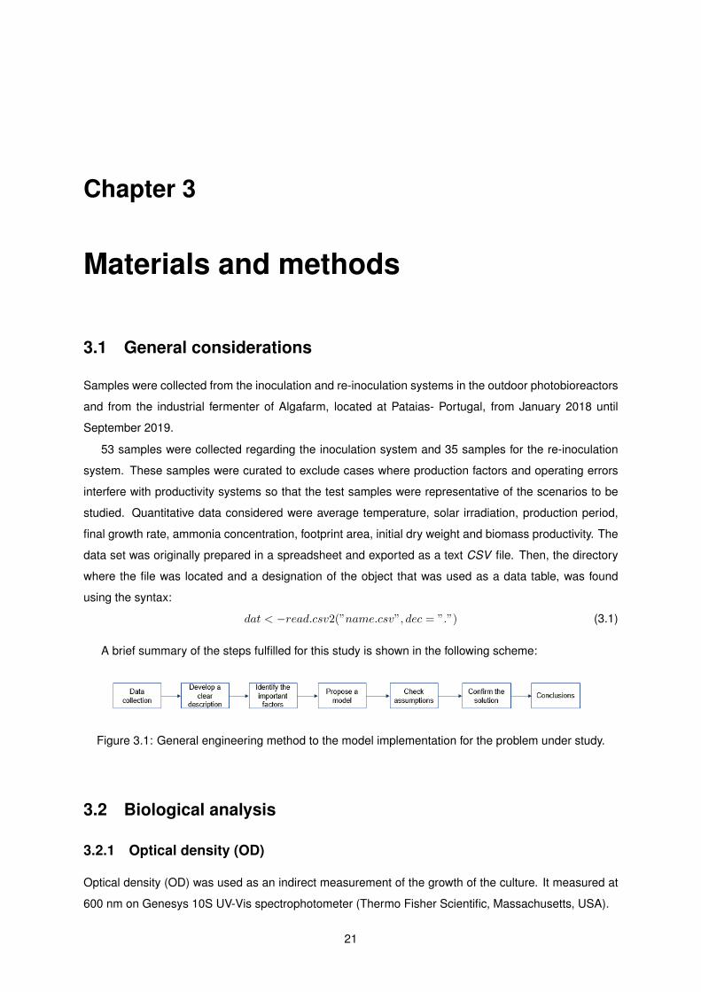
A brief summary of the steps fulfilled for this study is shown in the following scheme:
Figure 3.1: General engineering method to the model implementation for the problem under study.
3.2 Biological analysis
3.2.1 Optical density (OD)
Optical density (OD) was used as an indirect measurement of the growth of the culture. It measured at
600 nm on Genesys 10S UV-Vis spectrophotometer (Thermo Fisher Scientific, Massachusetts, USA).
21
3.2.2 Dry weight
Dry weight (DW) was determined by filtering a defined volume of a given sample in microglass filters
(0.7 µm, VWR, Almada, Portugal), which was washed with an equal volume of distilled water and dried
at 120◦ C using a DBS 60-30 electronic moisture analyzer (KERN SOHN GmbH, Balingen - Germany).
When DW of some old samples was not available, it was obtained using a calibration curve, which can
be seen in Appendix A, and was given by equation (3.2).
OD600 = 2.2803DW (g/L) + 0.0929 (R2 = 0.937) (3.2)
3.3 Chemical analysis
3.3.1 Ammonia concentration
Samples collected from the industrial fermenter were centrifuged to separate the supernatant. Next, the
Ammonia concentration in the supernatant was determined using an Ammonium-Ammonia Sera test
(Sera, Heinsberg, Germany) following manufacturer instructions.At last,OD was read at 697 nm using
a Genesys 10S UV-Vis spectrophotometer (Thermo Fisher Scientific, Massachusetts, USA). The result
was compared to calibration curve to obtain the ammonia concentration.
3.4 Data analysis
3.4.1 Software
Data analysis was performed using an open source software, R version 3.5.3. R. All the packages
required for the analysis were downloaded at the Comprehensive R Archive Network (CRAN) [98].
Moreover, RStudio was used as an integrated development environment for R. The fulltext editor and
the tab compilation of file name, function name and argument were also done in this interface.
3.4.2 Statistical analysis
In Principal Component Analysis, individuals and variables factor map were given by the PCA() function
from the FactoMineR package. In PCA() the data were scaled to unit variance and returned the matrix
containing all the eigenvalues, the percentage of variance, the cumulative percentage of variance and
the contributions of the variables to the principal components. Missing values were replaced by the
column mean. In addition, dimdesc function was used to identify the variables that are the most charac-
teristic according to each dimension. The package Factoextra was requested to color the variables by
the value of their contributions.
22

3.4.3 Regression analysis
The graphical display of the correlation matrices was performed using the corrplot function. The pro-
ductivity was considered the dependent variable. The correlation values between independent and
dependent variables were produced independently by cor function. Pearson method’s was used by
default.
The packages required for the multiple linear model implementation were: car, lme4 and visreg.
Fitting model was achieved by the function lm. The syntax to obtain the model was:
model1 < −lm(response variable ∼ independent variables, data = dat) (3.3)
The packages required for the generalized least squares model implementation was nlme. The fitting
model was achieved by the function gls and its respective variance structure. The syntax to obtain the
model was:
mod1 < −gls(response variable ∼ independent variables, weights = () data = dat) (3.4)
vf1 < −varFunc(∼ independentvariable) (3.5)
The model results were given using the command summary(model1). Before considering and ac-
cepting the results of the obtained linear model, Shapiro-Wilk test was the normality test performed using
shapiro.test function, the variance inflation factor was calculated by the function vif and the autocorrela-
tion was tested by durbinWatsonTest. The significance level of 5 % was used for the assumption tests.
The plot() function gave the graphs for the residuals . The standard Anova function was used to do the
analysis of variance.
Furthermore, to test the quality of statistical models, AIC function was used.
The function visreg was applied to visualize the regression models, returning plots containing a
confidence band, prediction line, and partial residuals.
Lastly, to check the predictive performance of the model, one validation strategy was assessed
through dplyr, caret, lattice and rpart packages. In this strategy, predict() function was implemented.
All the necessary R scripts for this study are described in appendix B.
3.4.4 Variables
Ammonia concentration
Ammonia concentration was measured at the time the culture in the industrial fermenter was ready
to seed the outdoor photobioreactors. This concentration was expressed in mM.
Final Specific Growth rate
23

The final specific growth rate, µ, was given by the equation (3.6) at the time the culture in the industrial
fermenter was ready to seed the outdoor photobioreactors.
µ(h−1) =ln(N2/N1)
t2 − t1(3.6)
Production period
Production period, in days, referred to the time of production inside the photobioreactors.
Footprint area
The footprint area corresponds to the photosynthetic exposed area in PBRs, in m2, and was obtained
by DraftSight 2D CAD Drafting R© and 3D Design R© softwares.
Incident radiation
Solar irradiance was continuously measured by WatchDog 2000 series weather station (Spectrum
Technologies, Aurora, IL, USA), in W/m2. This probe was located near the photobioreactors. Solar
irradiance was integrated with the probe measurements over a given time period to obtain the radiant
energy in J/m2 emitted during that daylight time period. Lastly, the total solar irradiation (J) was calcu-
lated by multiplying radiant energy by the footprint area of the PBR. The radiation used in the model was
given in MJ/day.
Average temperature
The culture temperature in ◦ C was continuously measured by a pH and temperature probe located
in the pump suction pipe in the PBR. The average temperature was calculated based on the mean
temperature during daylight hours divided by the production period. Time for sunrise and sunset of
Pataias, Portugal was defined based on website sunrise-and-sunset [99].
Initial dry weight
Initial biomass concentration, expressed in g/L was obtained as described in 3.2.2, expressed the
concentration of the culture on outdoor photobioreactors, after inoculation or re-inoculation processes.
Biomass productivity
Volumetric biomass productivity in the photobioreactors was calculated based on equation (3.7) for
each production period (between ti and tf , corresponding to initial and final time, respectively), consid-
ering the respective DW (g/L).
P (g.L−1.day−1) =DWf −DWi
tf − ti(3.7)
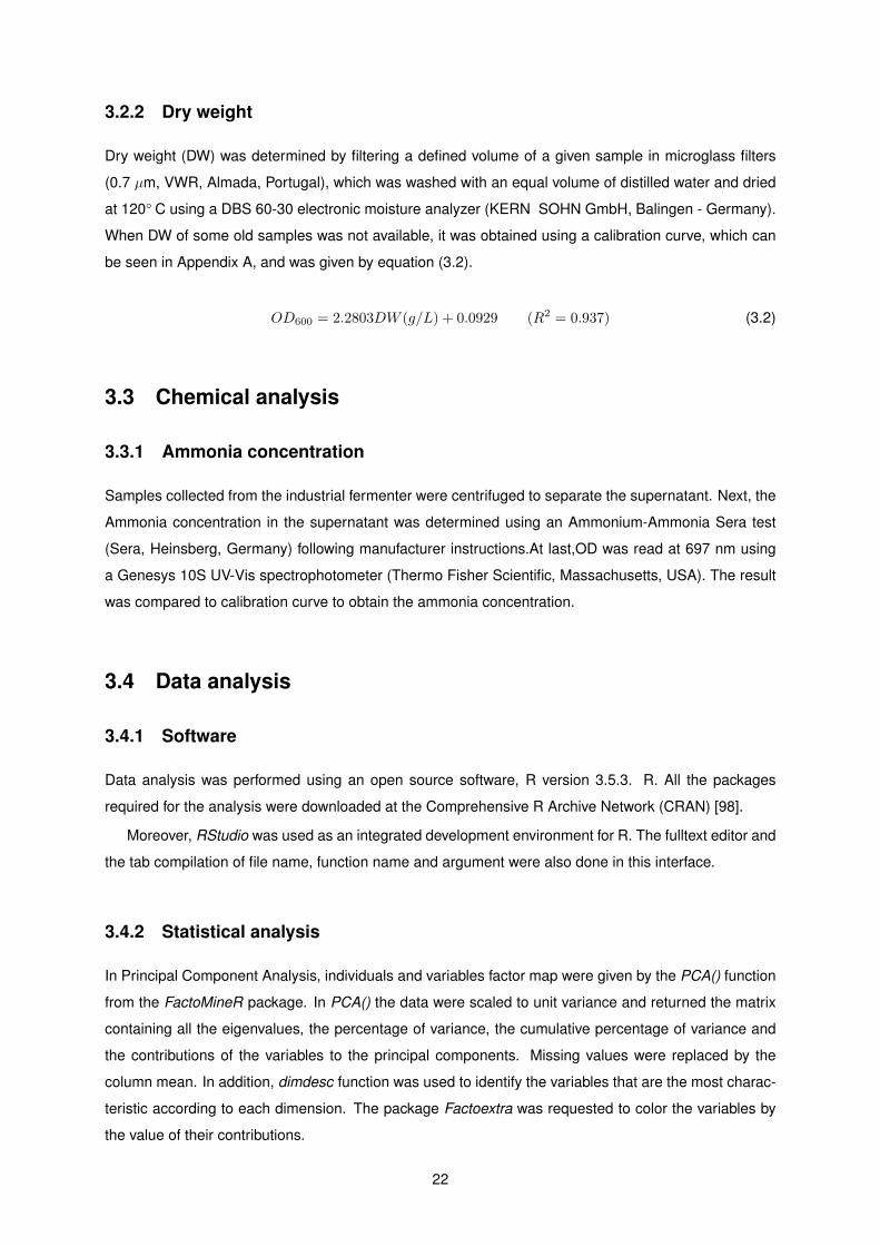
As those variables are involved in Allmicroalgae’s production context, the figure 3.2 shows where the
variables were collected in the process.
24
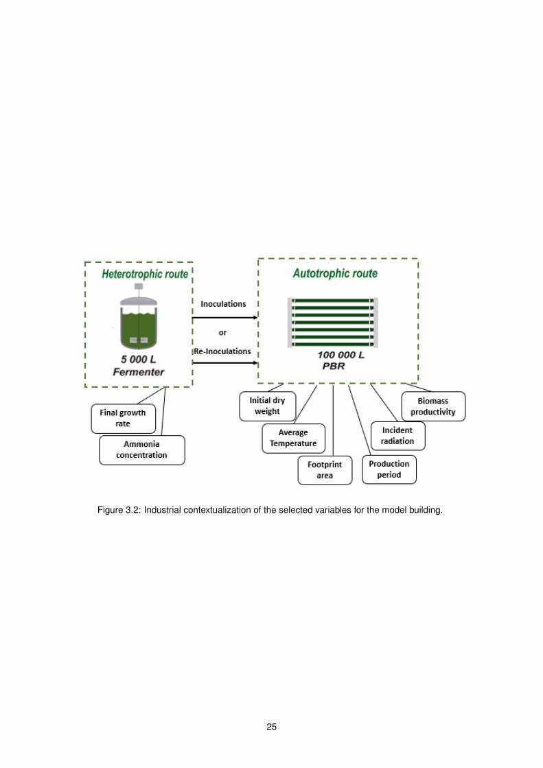
Figure 3.2: Industrial contextualization of the selected variables for the model building.
25

26

Chapter 4
Results and discussion
4.1 Principal component analysis
4.1.1 General PCA Classification Scheme
Allmicroalgae has a heterotrophic/autotrophic sequential Chlorella vulgaris cultivation method, inocu-
lating and re-inoculating photobioreactors from the industrial fermenter. Thus, cultures productivity in
PBRs is influenced by several factors. To visualize the effect of these different factors on biomass pro-
ductivity, PCA plots were built and analyzed. The first step of constructing PCA plots was to construct
a correlation matrix using the data set of 44 samples for inoculation and another data set of 32 sam-
ples for re-inoculation systems and their corresponding seven influence factors on productivity. Then
the eigenvalues of the correlation matrix were calculated. The number of principal components with
practical significance was determined using eigenvalues. Finally, a variables factor map which shows
the structural relationship between the variables and the components helping to name the components
was generated. The variables factor map also allowed reading the correlation between the variable and
the component.
4.1.2 Inoculation systems
4.1.2.1 Classification using Eigenvalues
The eigenvalues resulted from the correlation matrix of the data set are listed in Table 4.1. The eight
eigenvalues presented are ordered from the highest to the lowest variance of the data set. The first
three principal components give 74 % of the total variability. According to the Scree Plot shown in Figure
4.1, it is not clear whether keeping two or three principal components was the best option. However, if
considering that choosing only two principal components, the total variance of the original data set is
reduced to 58%, the data matrix is described by three principal components.
27
Table 4.1: Eigenvalues, percentage of variance and cumulative percentage of the correlation matrix ofthe principal component analysis for inoculation systems.
PrincipalComponent
Eigenvalue Variance %Cumulative
Variance (%)
1 2.707 33.8 33.82 1.930 24.1 583 1.279 16 744 0.988 12.4 86.35 0.450 5.6 91.96 0.295 3.7 95.67 0.250 3.1 98.88 0.100 1.2 100
Figure 4.1: Scree Plot of PCA eigenvalues for data analyzed in inoculation systems.
4.1.2.2 Special features of the PCA plot
PCA is a useful tool for visualizing the correlation between original variables. For those reasons, it has
been applied to biological systems in order to extract important information which is not directly seen.
The contributions of variables to the first three principal components are shown in Figure 4.2, which
shows that the variables final growth rate, temperature and productivity are the ones contributing the
most to the first three dimensions.
Figure 4.3 shows the factor maps which help to visualize clusters of correlated variables. The first
principal component explains 33.8% of the total variation, and the second principal component an addi-
tional 24.1%. In the first dimension, the variable productivity was positively correlated with environmental
conditions (temperature and radiation) which indicates that biomass productivity in the photobioreactors
(PBRs) is highly dependent on those conditions [100]. It was already described that outdoor photobiore-
actors are usually naturally illuminated using solar light, indicating that biomass productivities depend
on the prevailing weather conditions [100]. The author Marıa Franco et al. (2012) has found significant
differences in C. vulgaris productivity when cultured during summer or winter periods, leading to a higher
28
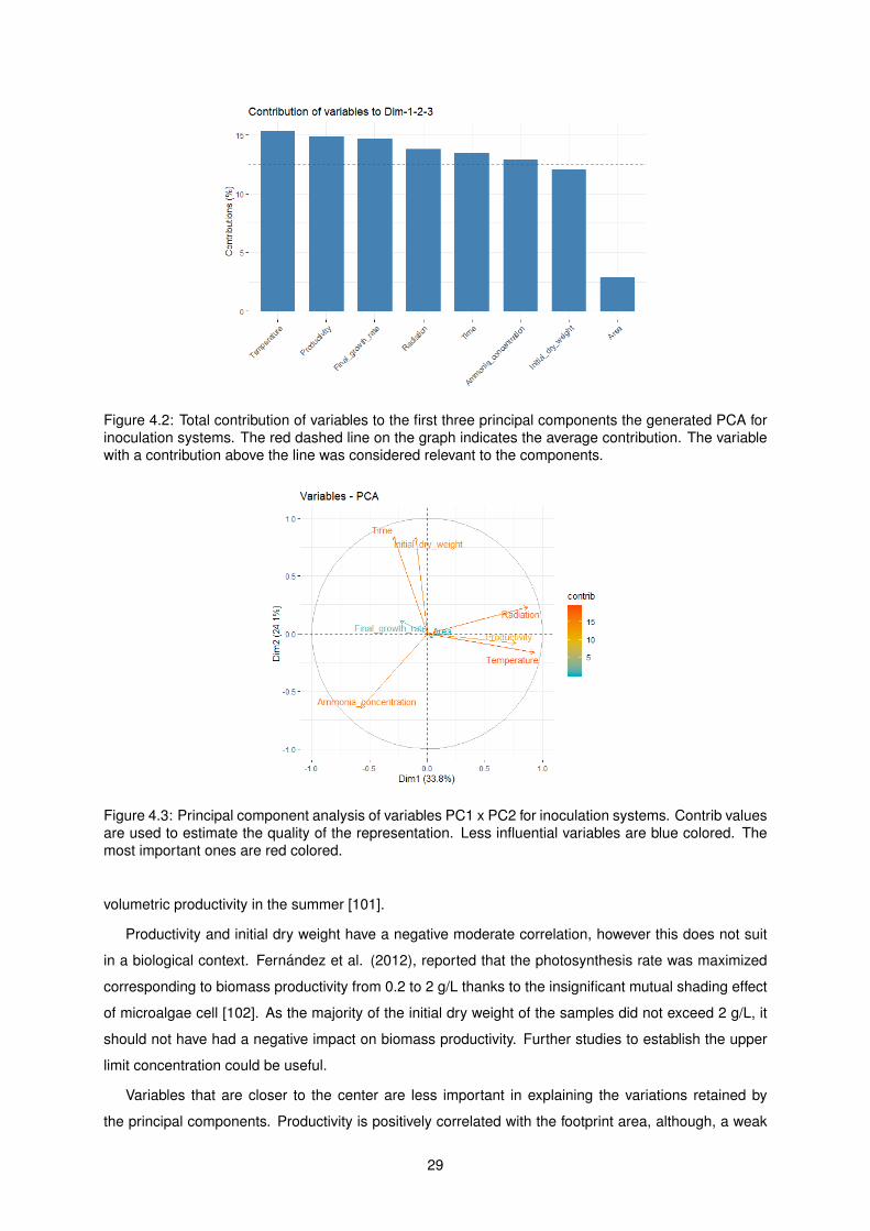
Figure 4.2: Total contribution of variables to the first three principal components the generated PCA forinoculation systems. The red dashed line on the graph indicates the average contribution. The variablewith a contribution above the line was considered relevant to the components.
Figure 4.3: Principal component analysis of variables PC1 x PC2 for inoculation systems. Contrib valuesare used to estimate the quality of the representation. Less influential variables are blue colored. Themost important ones are red colored.
volumetric productivity in the summer [101].
Productivity and initial dry weight have a negative moderate correlation, however this does not suit
in a biological context. Fernandez et al. (2012), reported that the photosynthesis rate was maximized
corresponding to biomass productivity from 0.2 to 2 g/L thanks to the insignificant mutual shading effect
of microalgae cell [102]. As the majority of the initial dry weight of the samples did not exceed 2 g/L, it
should not have had a negative impact on biomass productivity. Further studies to establish the upper
limit concentration could be useful.
Variables that are closer to the center are less important in explaining the variations retained by
the principal components. Productivity is positively correlated with the footprint area, although, a weak
29

correlation is seen. Ammonia concentration is almost orthogonal with the variable productivity, indicating
that it do not influence this variable.
A strong and positive correlation between time and initial dry weight does not seem to be biologically
related.
A negatively correlation between final growth rate and productivity was also showed by the first
dimension. It was observed by Mattos ER et al. (2012) that different physiological stages in the inoculum
obtained different biomass production [103].
For further assays, it was considered that just temperature and the final growth rate have a relevant
biological impact on productivity.
4.1.3 Re-inoculation systems
The eigenvalues resulted from the correlation matrix of the data set are presented in Table 4.2. The
firsts three principal components gave 66 % of the total variance. According to the Scree Plot shown in
Figure 4.1, it was also not clear whether keeping two or three principal components represented better
the reality. However, when keeping only two principal components, the total variance of the original data
set was reduced to 50%. For this reason, the data matrix was described by the three most significant
principal components.
Table 4.2: Eigenvalues, percentage of variance and cumulative percentage of the correlation matrix ofthe principal component analysis for re-inoculation systems.
PrincipalComponent
Eigenvalue Variance %Cumulative
Variance (%)
1 2.213 27.7 27.72 1.801 22.5 50.23 1.252 15.7 65.84 1.027 12.8 78.75 0.624 7.8 86.56 0.554 6.9 93.47 0.359 4.5 97.98 0.171 2.1 100
4.1.3.1 Special features of the PCA plot
The contributions of variables to the first three principal components are shown in Figure 4.5. The plot
is clear showing that the variables initial dry weight, temperature, and productivity contribute the most to
the first three dimensions.
A factor map is presented in Figure 4.6, which helps to visualize the cluster of correlated variables.
In this case, the first principal component explained 27.1% of the total variation, the second principal
component 22.1%, and the third principal component an additional 16.6%. The first dimension explains
that productivity and temperature are the most contributing variables. These two variables are also
highly negatively correlated with each other. This correlation was attributed to a operational reason,
30
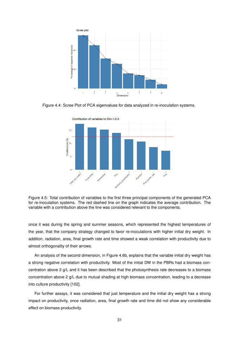
Figure 4.4: Scree Plot of PCA eigenvalues for data analyzed in re-inoculation systems.
Figure 4.5: Total contribution of variables to the first three principal components of the generated PCAfor re-inoculation systems. The red dashed line on the graph indicates the average contribution. Thevariable with a contribution above the line was considered relevant to the components.
once it was during the spring and summer seasons, which represented the highest temperatures of
the year, that the company strategy changed to favor re-inoculations with higher initial dry weight. In
addition, radiation, area, final growth rate and time showed a weak correlation with productivity due to
almost orthogonality of their arrows.
An analysis of the second dimension, in Figure 4.6b, explains that the variable initial dry weight has
a strong negative correlation with productivity. Most of the initial DW in the PBRs had a biomass con-
centration above 2 g/L and it has been described that the photosynthesis rate decreases to a biomass
concentration above 2 g/L due to mutual shading at high biomass concentration, leading to a decrease
into culture productivity [102].
For further assays, it was considered that just temperature and the initial dry weight has a strong
impact on productivity, once radiation, area, final growth rate and time did not show any considerable
effect on biomass productivity.
31

(a) (b)
Figure 4.6: Principal component analysis of variables (PC1 x PC2) (a) and (PC2 x PC3) (b) for re-inoculation systems. Contrib values are used to estimate the quality of the representation. Less impor-tant variables are coloured by blue. The most important ones are coloured by red.
4.1.4 Comparing inoculation with re-inoculation systems
Regarding ammonia concentration variable, both systems allowed to conclude that it does not have an
influence on productivity. Tam NFY and Wong YS (1996) reported that, for C. vulgaris, growth occurred
in ammonia concentrations between 1 to 60 mM. At high ammonia concentrations (60 mM) cell division
was inhibited, however, such concentrations did not cause any visible lethal effect [104]. Once, nearly
70% of the data set for both systems presented values of ammonia in that range, it was possible to infer
that this variable did not affect biomass productivity, not being a limiting factor.
The footprint area also did not reveal any significant influence on biomass productivity, which should
be due to the fact the footprint area of the PBRs in this study ranged from 482 to 502 m2. According to
Hu et al. (1998), the increase of illumination surface area provides higher photosynthetic efficiency and
consequently higher growth rate [105]. However, the differences between the surfaces area of the PBRs
used for this work did not seem to be significant. That fact should be further confirmed.
The production period (time) in the PBRs did not show any influence in biomass productivity for re-
inoculation systems. However, it showed a negative moderate correlation with productivity in inoculation
systems. Since production period was already incorporated in productivity calculations, it should not
have had any impact on productivity. Further studies in re-inoculations should include the production
time period of the culture already in the PBRs.
Differences between the total variability in both systems, in the first three principal components, 74%
for inoculation and just 66% for re-inoculation may assume older cultures conditions in PBRs produc-
tion had an impact on the biomass productivity in case of re-inoculations, because culture from the
heterotrophic production besides adapting to the new autotrophic environment it also had to adapt to
the culture already in production in PBRs. This cultures may have been at different growth stages and
diverse different culture conditions. Furthermore, outdoor cultivation systems with high volumes such as
Allmicroalgae PBRs have great variability.
32

4.2 Regression- Construction of a predictive equation for inocu-
lation and re-inoculation system in photobioreactors
4.2.1 General Regression Classification Scheme
This section aimed mainly to build multiple regression equations that enable to predict the biomass
productivity (dependent variable) considering one or more independent variables for both inoculation
and re-inoculation systems. The independent variables considered were final ammonia concentration
and final growth rate in the fermenter; time period, footprint area, temperature, radiation and initial dry
weight in the photobioreactors. The data set used in this section was the same as the one used in
section 4.1, consisting of 50 independent samples. From this set, and after deleting outliers, 80% of the
data was taken as the training set and the other 20% was considered as the validation set in order to
check the viability this regression as a predictive model. The same process was taken into account for
re-inoculation systems with a data set of 32 samples. However, besides this division, the final model for
inoculation and re-inoculation systems include both the data from training and testing.
4.2.2 Inoculation systems
4.2.2.1 Correlation between variables
In order to verify the influence of the various factors a scatter plot matrix and a correlation plot of the
data set were computed and analyzed.
Figure 4.7: Correlation matrix between the variables in inoculation systems. Positive correlations aredisplayed in blue and negative correlations in red color. Color intensity is equivalent to the correlationcoefficients. Abbreviations meaning: temp- temperature, radi- radiation, fgrf- final growth rate, idrw-initial dry weight, famc- ammonia concentration, prod- productivity
33
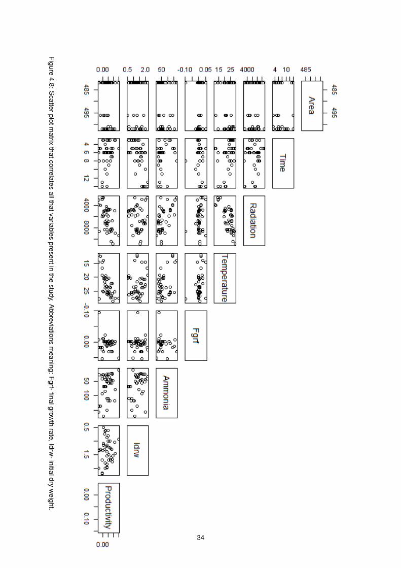
Figure4.8:
Scatterplotm
atrixthatcorrelates
allthatvariablespresentin
thestudy.
Abbreviations
meaning:
Fgrf-finalgrowth
rate,Idrw-initialdry
weight.
34
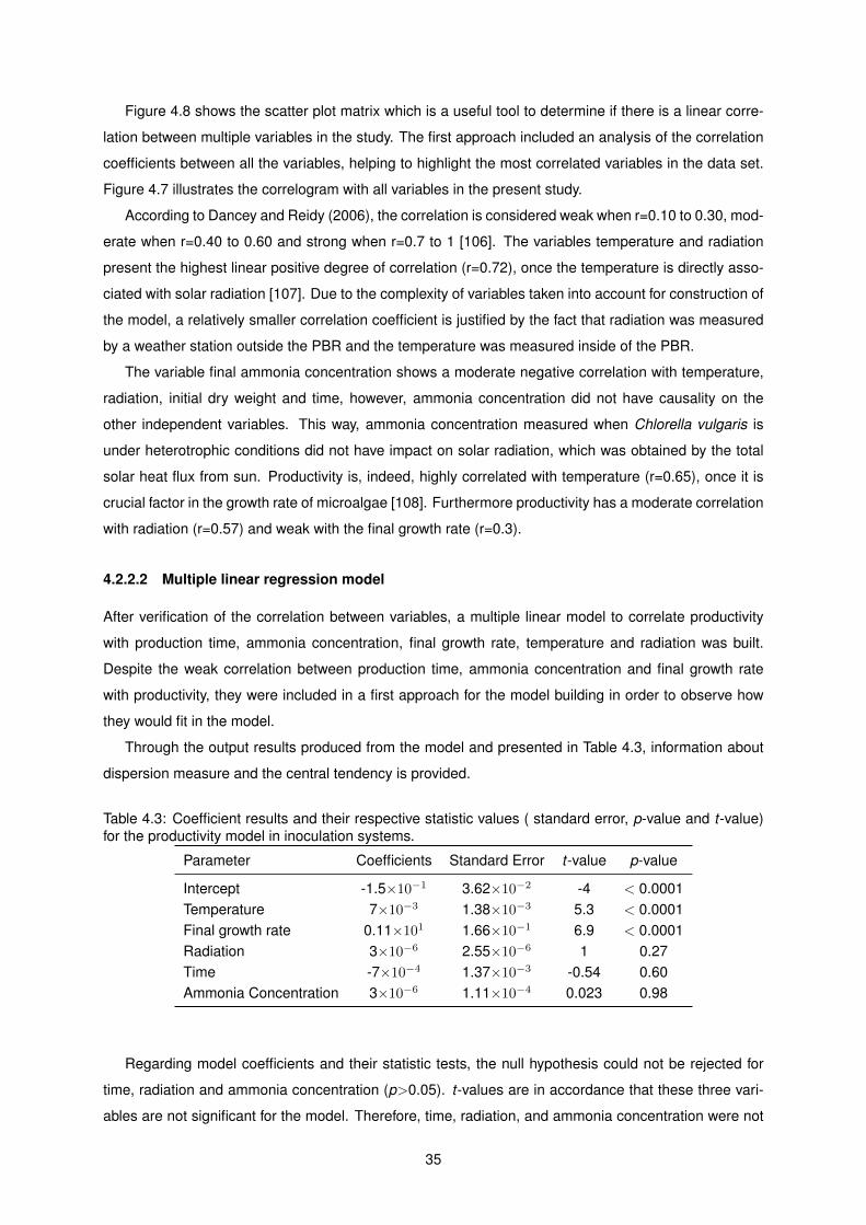
Figure 4.8 shows the scatter plot matrix which is a useful tool to determine if there is a linear corre-
lation between multiple variables in the study. The first approach included an analysis of the correlation
coefficients between all the variables, helping to highlight the most correlated variables in the data set.
Figure 4.7 illustrates the correlogram with all variables in the present study.
According to Dancey and Reidy (2006), the correlation is considered weak when r=0.10 to 0.30, mod-
erate when r=0.40 to 0.60 and strong when r=0.7 to 1 [106]. The variables temperature and radiation
present the highest linear positive degree of correlation (r=0.72), once the temperature is directly asso-
ciated with solar radiation [107]. Due to the complexity of variables taken into account for construction of
the model, a relatively smaller correlation coefficient is justified by the fact that radiation was measured
by a weather station outside the PBR and the temperature was measured inside of the PBR.
The variable final ammonia concentration shows a moderate negative correlation with temperature,
radiation, initial dry weight and time, however, ammonia concentration did not have causality on the
other independent variables. This way, ammonia concentration measured when Chlorella vulgaris is
under heterotrophic conditions did not have impact on solar radiation, which was obtained by the total
solar heat flux from sun. Productivity is, indeed, highly correlated with temperature (r=0.65), once it is
crucial factor in the growth rate of microalgae [108]. Furthermore productivity has a moderate correlation
with radiation (r=0.57) and weak with the final growth rate (r=0.3).
4.2.2.2 Multiple linear regression model
After verification of the correlation between variables, a multiple linear model to correlate productivity
with production time, ammonia concentration, final growth rate, temperature and radiation was built.
Despite the weak correlation between production time, ammonia concentration and final growth rate
with productivity, they were included in a first approach for the model building in order to observe how
they would fit in the model.
Through the output results produced from the model and presented in Table 4.3, information about
dispersion measure and the central tendency is provided.
Table 4.3: Coefficient results and their respective statistic values ( standard error, p-value and t-value)for the productivity model in inoculation systems.
Parameter Coefficients Standard Error t-value p-value
Intercept -1.5×10⁻¹ 3.62×10⁻² -4 < 0.0001Temperature 7×10⁻³ 1.38×10⁻³ 5.3 < 0.0001Final growth rate 0.11×101 1.66×10⁻¹ 6.9 < 0.0001Radiation 3×10⁻⁶ 2.55×10⁻⁶ 1 0.27Time -7×10⁻⁴ 1.37×10⁻³ -0.54 0.60Ammonia Concentration 3×10⁻⁶ 1.11×10⁻⁴ 0.023 0.98
Regarding model coefficients and their statistic tests, the null hypothesis could not be rejected for
time, radiation and ammonia concentration (p>0.05). t-values are in accordance that these three vari-
ables are not significant for the model. Therefore, time, radiation, and ammonia concentration were not
35

included in the final model. In the particular case of radiation that has a moderate correlation coefficient
with productivity in the correlation matrix, here t-value=1, meaning a powerless influence regarding the
dependent variable. Furthermore, radiation would not be a useful variable in predictive models since it
cannot be predicted from the weather conditions.
The output produced in R also indicates R2 = 0.76 and R2 adjusted =0.73. For this model, about
73% of the productivity can be adjusted to the linear model.
Since productivity seems to be influenced just by, mainly, two variables, a second model was tested
with the AIC value to compare the quality of models. First model AIC value was -204.5 and for the
new model was -208.9, giving the information that the depletion of time, ammonia concentration and
radiation, did not affect the quality of the new model. The process of excluding variables and adapting
the initial model must take into account the context of the problem and the importance of these variables
in the biological context, not just from a mathematical perspective. Besides ammonia concentration and
production time did not have statistical significance in regression, they also did not show a biological
impact in biomass productivity as mentioned before in section 4.1.2.2.
Thus, the new linear model was achieved, including temperature and final growth rate as independent
variables and whose coefficient of determination values are approximately identical to the first model.
Table 4.4 provides information about the coefficients and their test statistics of the new model. Additional
important information about the overall model is showed in Table 4.5.
Table 4.4: Coefficient results and their respective statistic values (standard error, p-value and t-value)of the new model for productivity in inoculation systems. P-values from the coefficients have the higherlevels of significance ***.
Parameter Coefficients Standard Error t-value p-value
Intercept -0.16 0.0189 -8.4 < 0.0001Temperature 0.0085 0.000805 10.6 < 0.0001Final growth rate 1.2 0.161 7.2 < 0.0001
Based on the coefficients, the linear model is described by the following equation:
y = −0.16 + 0.0085x1 + 1.2x2 R2 = 0.753 (4.1)
where y = productivity, x1=temperature and x2= final growth rate.
Table 4.5: Residuals results for the productivity model in inoculation systems.
Model Residual standard Error Degrees of freedom R2 R2adj F-value p-value
Inoculation system 0.021 41 0.753 0.741 63 < 0.0001
According to the Table 4.5, an F-statistic value of 63 is big enough to reject the null hypothesis,
showing that there was a relationship between productivity and the independent variables. The residual
standard error, which represents the average amount that the productivity deviates from the true regres-
sion line, was 0.021. 74% of the productivity variable can be adjusted to the linear model, presenting
36
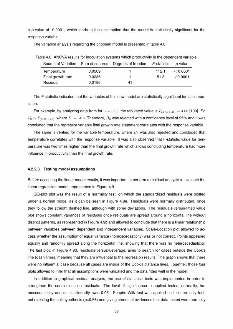
a p-value of 0.0001, which leads to the assumption that the model is statistically significant for the
response variable.
The variance analysis regarding the choosen model is presented in table 4.6.
Table 4.6: ANOVA results for inoculation systems which productivity is the dependent variable.
Source of Variation Sum of squares Degrees of freedom F -statistic p-value
Temperature 0.0509 1 112.1 < 0.0001Final growth rate 0.0235 1 51.8 <0.0001Residual 0.0186 41
The F statistic indicated that the variables of this new model are statistically significant for its compo-
sition.
For example, by analyzing data from for α = 0.05, the tabulated value is F(0.95;1;41) = 4.08 [109]. So
F0 > F(0.95;1;41), where F0 = 51.8. Therefore, H0 was rejected with a confidence level of 95% and it was
concluded that the regressor variable final growth rate statement correlates with the response variable.
The same is verified for the variable temperature, where H0 was also rejected and concluded that
temperature correlates with the response variable. It was also observed that F-statistic value for tem-
perature was two times higher than the final growth rate which allows concluding temperature had more
influence in productivity than the final growth rate.
4.2.2.3 Testing model assumptions
Before accepting the linear model results, it was important to perform a residual analysis to evaluate the
linear regression model, represented in Figure 4.9.
QQ-plot plot was the result of a normality test, on which the standardized residuals were plotted
under a normal mode, as it can be seen in Figure 4.9a. Residuals were normally distributed, once
they follow the straight dashed line, although with some deviations. The residuals-versus-fitted value
plot shows constant variances of residuals once residuals are spread around a horizontal line without
distinct patterns, as represented in Figure 4.9b and allowed to conclude that there is a linear relationship
between variables between dependent and independent variables. Scale-Location plot allowed to ac-
cess whether the assumption of equal variance (homoscedasticity) was or not correct. Points appeared
equally and randomly spread along the horizontal line, showing that there was no heteroscedasticity.
The last plot, in Figure 4.9d, residuals-versus-Leverage, aims to search for cases outside the Cook’s
line (dash lines), meaning that they are influential to the regression results. The graph shows that there
were no influential case because all cases are inside of the Cook’s distance lines. Together, those four
plots allowed to infer that all assumptions were validated and the data fitted well in the model.
In addition to graphical residual analysis, the use of statistical tests was implemented in order to
strengthen the conclusions on residuals. The level of significance in applied testes, normality, ho-
moscedasticity and multicollinearity, was 0.05. Shapiro-Wilk test was applied as the normality test,
not rejecting the null hypothesis (p=0.56) and giving shreds of evidences that data tested were normally
37

(a) (b)
(c) (d)
Figure 4.9: Diagnostic Plots of Multiple Linear Regression Model for inoculation systems.
distributed. Breusch-Pagan test was applied to check homoscedasticity of residuals, allowing to con-
sider the null hypothesis was not rejected (p=0.21), and so, it was possible to infer that the variance of
residuals is constant. To detect multicollinearity, the VIF score was computed (VIF=1), leading to the
conclusion that, by the rule of thumb, there is the absence of multicollinearity. Last, Durbin-Watson test
was also not rejected (p=0.78), therefore, there is no autocorrelation in the residuals.
Hence, the multiple linear regression model fulfills the required assumptions for the statistical vali-
dation’s model and for performing statistically valid inference. Note that the initial model underwent the
same tests and the results were similar.
Figure 4.10 shows how the expected value of productivity changed as function of temperature or
final growth rate, with all other variables in the model held fixed. The productivity is maximum presented
at, nearly, 28◦ C. Those results are in accordance with M. Huesemann and B. Crowe (2013), which re-
ported a positive linear relationship between maximum growth rate of C. vulgaris and temperature for
the ranges 13◦ C to 36◦ C, exhibiting a higher maximum growth rate at 36◦ C [110]. Moreover, Figure
4.10b observations can lead to the conclusion that productivity is directly proportional to the tempera-
38

(a) (b)
Figure 4.10: Plots of the fitted model in terms how the variables final growth rate (a) and temperature (b)were estimated to affect the productivity for inoculation systems. The blue line indicates the expectedvalue, the gray band a confidence interval for the expected value and the dark gray dots the partialresiduals.
ture. In addition, in Allmicroalgae, the inoculum from the industrial fermenter is used used to inoculate
photobioreactors, mostly, when in the exponential phase. Figure 4.10a demonstrates that as long as the
growth rate increased the higher was the productivity. According to Erico R. Mattos et al. (2012), there
is a natural advantage of this stage because of the increased amount of medium size cells multiplying
at a high rate, explaining such high productivities [103].
4.2.3 Re-inoculation systems
4.2.3.1 Correlation between variables
The construction of a predictive model for re-inoculation systems was carried out following the same
procedure as on inoculation systems.
39

Figure 4.11: Correlation matrix between the variables in re-inoculation systems. Abbreviations mean-ing: temp- temperature, radi- radiation, fgrf- final growth rate, idrw- initial dry weight, famc- ammoniaconcentration, prod- productivity.
The visualization of the scatter plot matrix, in Figure 4.12, and correlation matrix, in Figure 4.11,
allowed determining the correlation between all the variables.
The highest correlation in the correlogram above was between productivity and initial dry weight
(r=-0.55), which was negative, indicating that as the biomass concentration at the inoculation point in-
creased, the productivity decreased, as mentioned in section 4.1.3.1. Temperature displayed a moderate
negative correlation (r=-0.43) with productivity, however, this was a consequence of deciding to inocu-
late at high biomass concentration during spring and summer seasons, already discussed in section
4.1.3.1. The variable time had a moderate correlation with temperature and ammonia concentration,
however, this variable did not have causality on these independent variables, once those two variables
are biologically independent.
The variables initial dry weight and temperature were the variables influencing the most biomass
productivity, as seen before in Section 4.1.3 This relationship between initial dry weight is due to mutual
shading above biomass concentration 2 g/L, leading to a decrease in culture productivity [102]. Regard-
ing the relationship between temperature and productivity, it was justified in the previous paragraph.
4.2.3.2 Multiple linear regression model
After verifying the correlation between variables, a first multiple linear model to correlate productivity
with production time, initial dry weight, temperature and radiation was built. The footprint area, ammonia
concentration and the final growth rate were not included in the model because their coefficients values
below were 20%.
40

Figu
re4.
12:
Sca
tterp
lotm
atrix
that
corr
elat
esal
ltha
tvar
iabl
espr
esen
tin
the
stud
y.A
bbre
viat
ions
mea
ning
:Fg
rf-fin
algr
owth
rate
,Idr
w-i
nitia
ldry
wei
ght.
41

Table 4.7: Coefficient results and their respective statistic values ( standard error, p-value and t-value)for the productivity model in re-inoculation systems.
Parameter Coefficients Standard Error t-value p-value
Intercept 7×10⁻¹ 1.52×10⁻¹ 4.7 < 0.0001Temperature -1.8×10⁻² 4.93×10⁻³ -3.6 < 0.0001Initial dry weight -1.3×10⁻¹ 2.70×10⁻² -4.9 < 0.0001Time 2×10⁻³ 4.90×10⁻³ 0.43 0.67Radiation -4×10⁻⁶ 3.42×10⁻⁶ -1 0.31
Regarding model coefficients and their statistic tests statistics presented in Table 4.7, the null hypoth-
esis was not reject in the case of radiation and time because their test statistics present p-values above
0.05. Although the t-value for radiation had a value of -1, it was not considered an important variable
for the model for the same reason as in section 4.2.2.2, once it becomes difficult to predict. The output
produced in R also indicates R2=0.62 and R2adj=0.56. About 56% of the productivity could be adjusted
to the linear model generated. For AIC value for the first model was -88.2 and the new model was -90.7,
clearly showing an increase in its quality.
Thus, the new linear model was achieved including temperature and initial dry weight as independent
variables. Table 4.8 provides information about new model’s the coefficients and their statistic tests.
Additional important information about the overall model is shown in Table 4.9.
Table 4.8: Coefficient results and their respective statistic values (standard error, p-value and t-value) ofthe new model for productivity in re-inoculation systems. P-values from the coefficients have the higherlevels of significance ***.
Parameter Coefficients Standard Error t-value p-value
Intercept 0.7 0.121 6.2 < 0.0001Temperature -0.019 0.0039 -4.8 < 0.0001Initial dry weight -0.14 0.025 -5.4 < 0.0001
Based on the coefficients, the produced linear model was described by the following equation:
y = 0.7− 0.019x1 − 0.14x2 R2 = 0.597 (4.2)
where y = productivity, x1=temperature and x2= initial dry weight.
Table 4.9: Residuals results of the model for productivity in re-inoculation systems.
Model Residual standard Error Degrees of freedom R2 R2adj F-statistic p-value
Re-inoculation system 0.055 27 0.597 0.569 11 < 0.0001
According to Table 4.9, an F-statistic value of 11 allowed to reject the null hypothesis, showing that
there is relationship between productivity and the independent variables. The residual standard er-
ror, which represents the average amount that the productivity deviates from the true regression line,
was 0.055. 57% of the productivity variable can be adjusted to the linear model, presenting a p-
42
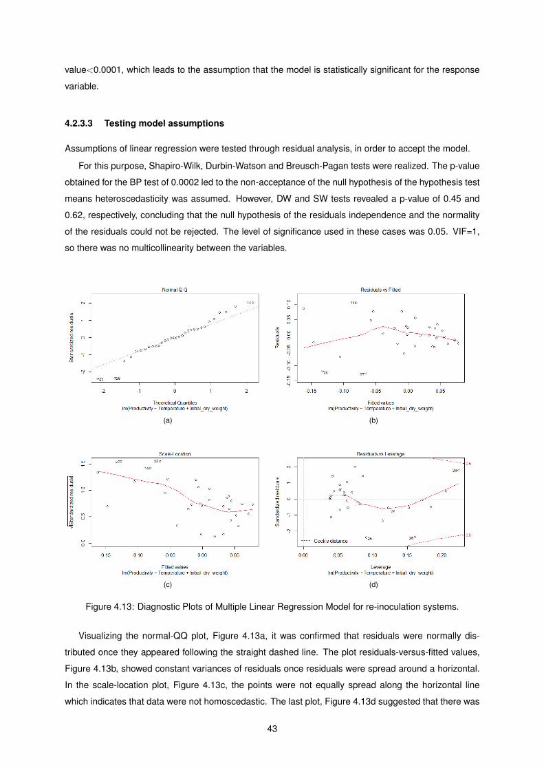
value<0.0001, which leads to the assumption that the model is statistically significant for the response
variable.
4.2.3.3 Testing model assumptions
Assumptions of linear regression were tested through residual analysis, in order to accept the model.
For this purpose, Shapiro-Wilk, Durbin-Watson and Breusch-Pagan tests were realized. The p-value
obtained for the BP test of 0.0002 led to the non-acceptance of the null hypothesis of the hypothesis test
means heteroscedasticity was assumed. However, DW and SW tests revealed a p-value of 0.45 and
0.62, respectively, concluding that the null hypothesis of the residuals independence and the normality
of the residuals could not be rejected. The level of significance used in these cases was 0.05. VIF=1,
so there was no multicollinearity between the variables.
(a) (b)
(c) (d)
Figure 4.13: Diagnostic Plots of Multiple Linear Regression Model for re-inoculation systems.
Visualizing the normal-QQ plot, Figure 4.13a, it was confirmed that residuals were normally dis-
tributed once they appeared following the straight dashed line. The plot residuals-versus-fitted values,
Figure 4.13b, showed constant variances of residuals once residuals were spread around a horizontal.
In the scale-location plot, Figure 4.13c, the points were not equally spread along the horizontal line
which indicates that data were not homoscedastic. The last plot, Figure 4.13d suggested that there was
43

no influential case because all cases were inside of Cook’s distance lines.
At this point, with the failure of homoscedasticity test, however with the normality of the data set was
ensured and it was no autocorrelation or multicollinearity in the model, an analysis of variance (ANOVA)
was not performed.
A non-constant error variance affected the properties of the OLS estimators and resulting test statis-
tics. Heteroscedasticity was corrected by the application of Generalized Least Square Models (GLS).
The parameters estimation of the GLS model fitted in the data set is as shown in Table 4.10.
Table 4.10: Parameter estimates of GLS model for productivity in re-inoculation systems.
Value Standard Error t-value p-value
Intercept 0.7 0.116 6.4 0Temperature -0.019 0.0036 -5.1 0Initial dry weight -0.14 0.025 -5.5 0
From the results seen in Table 4.10, both of the regressor variables (temperature and initial dry
weight) have p-values bellow 0.05 and therefore they are allow explaining the dependent variable (pro-
ductivity) of the data set. Both temperature and initial dry weight influenced productivity negatively as
their associated coefficients have a negative magnitude.
The resulting fitted GLS model was:
Y = 0.7− 0.019X1 − 0.14X2 (4.3)
Where, Y= productivity, X1= temperature and X2= Initial dry weight.
Table 4.11: Residuals results of the GLS model for productivity in re-inoculation systems.
Model Residual standard Error Degrees of freedom R2 R2adj
Re-inoculation system 0.011 32 0.593 0.565
According to Table 4.11, residual standard error, which represents the average amount that real
productivity deviates from the regression line, was 0.011 concluding a smaller deviation of productivity in
generalized least squares model. 57% of the productivity variable could be adjusted to the linear model,
presenting a p-value<0.0001, leading to the assumption that the model is statistically significant for the
response variable.
Regarding the assumptions of generalized least squares regression, it allowed for heteroscedasticity.
All other assumptions were remained to hold.
Figure 4.14 shows how the expected value of productivity changed as a function of temperature or
initial dry weight, with all other variables in the model held fixed. The high number of negative biomass
productivities in re-inoculation systems can be explained by the photosynthetic inhibition due to the high
cell concentration when inoculated [111]. Culture from industrial heterotrophic cultivation is seeded to
photobioreactors mainly to increase protein and chlorophyll contents. However, since cultures circulat-
ing in PBRs presents a significant cost in the whole microalgae production pipeline, it becomes of great
44

(a) (b)
Figure 4.14: Plots of the fitted model in terms of how the variables Temperature (a) and Initial dryweight (b) were estimated to affect the productivity for re-inoculation systems. The blue line indicatesthe expected value and the dark gray dots the partial residuals.
importance to maximize its productivity. Figure 4.14b demonstrates that as long as the initial DW in-
creased, the lower was the productivity values. Moreover, negative productivities were mainly observed
up to a biomass concentration of 2 g/L. In Figure 4.14a, as mentioned before, a decrease in biomass
productivity with the increase of temperature may be actually correlated to the other limiting factor - the
initial biomass concentration.
4.2.4 Comparison of the performance of the predictive models
Since the main purpose of the model was a prediction, accessing accuracy of the model in the context
of a real situation becomes mandatory. The strategy implemented aimed to overcome the problem of
overfitting: Hold Out Cross Validation Method. The performance of the two models were compared by
the presented three commonly used error measures- the mean absolute error (MAE) and the root mean
squared error (RMSE). In Table 4.12 are shown the results of the productivity error of the predictive
model for both inoculation systems.
Table 4.12: A comparison of the results of the productivity error of the predictive model for both inocula-tion systems.
Type of system RMSE train RMSE test MAE train MAE test
Inoculation 0.033 0.018 0.025 0.014
Re-inoculation 0.056 0.029 0.043 0.022
As seen from Table 4.12, inoculation systems across the training and testing set have smaller RMSE
and MAE compared to re-inoculation systems. Combining also a R2 of 73% for inoculation testing set
and a R2 of 63% for re- inoculation systems, it is clear that inoculation systems forecast better than
re-inoculation. This should be to the fact that in re-inoculation systems when sent to the PBR, the seed
culture had also to adapt to the culture already in production. Therefore, cells growing at two different
45

growth phases face a barrier to adaptation. Furthermore, successive re-inoculations are done in the
same PBR, adding even more biological variability factors to the culture growth. When reaching a suffi-
ciently high cell density, a process called Quorum sensing (QS) allows microorganisms to communicate
among them. These microorganisms can release chemical signal molecules, named autoinducers, that
increase in concentration as a function of cell density [112]. QS affects some microalgae physiological
features such as nutrient acquisition, biofilm formation, and self-motility. For example, QS enables ac-
cess of symbionts to nutrient-rich environments in hosts [113]. Chemotaxis allows microorganisms to
swim toward ideal conditions, thus providing microorganism with a competitive advantage in obtaining
nutrition in natural environments [114]. Cultures already in production have more experience in that en-
vironment than the new ones. Through QS factors, older cultures can cooperate with the new cultures,
having a synergistic effect- helping in the new cultures grow and producing faster more pigment and
protein content, or would may limit the growth of the new cultures.
Once productivity values ranged from -0.063 to 0.12, it was concluded that the lower values of RMSE
represented a good accuracy of the model. However, in re-inoculation systems productivity values
ranged from -0.19 to 0.079, which when compared to RMSE values of 0.056 and 0.029 for testing
and training data, respectively, less accuracy for re-inoculations was seen. Otherwise, both systems
presented lower RMSE on the testing when compared to training RMSE, indicating that both models
have a major predictive value when tested on new data. The Figure 4.15 shows the performance of
productivity obtained from the models and from the real productivity in the photobioreactors for both
inoculation systems.
Figure 4.15: The performance result of productivity obtained from the models and from the real produc-tivity in the photobioreactors for each sample in inoculation (a) and re-inoculation (b) systems.
It can be seen from Figure 4.15, the value of predictive productivity is close to the value of real
productivity. Results show that the overall accuracy of the influencing factors was 75.3% and 59.3% for
inoculation and re-inoculation systems, respectively, and for this reason they can be used to estimate
productivity. The predictive value of productivity is closer to the value of real productivity in inoculation
than in re-inoculation and also the R2 of inoculation is higher than in re-inoculation systems, as can be
noted on Figure 4.15. C. Webster Andrews et al. (2000) developed a quantitative structure-bioavailability
relationship model for drug discovery and development with an accuracy of 71.0% [115], Val H. Smith
46

(1985) suggested a predictive model for the biomass of blue-green algae in lakes depending on the
concentration of total phosphorus and the mean depth of the lake with an accuracy of 79.4% [116].
Therefore, as the accuracy of the developed models is within literature values, they represent a good
estimation of productivity based on the studied independent variables.
47

48

Chapter 5
Conclusions
5.1 Achievements
Productivity depends on a large number of variables due to the complexity of the biological system. To
better understand this type of system, the significant data must be selected from the large amount that is
available in order to capture the important information. In this dissertation, a free programming language
was used, R, for statistical computing and graphics. Statistical techniques are already implemented in
the software. The constant updating of statistical packages and mathematics, in general, make this tool
a crucial one for scientific research, since it is a language widely used by the international scientific
community.
The principal component analysis is, indeed, a useful statistical method to extract special features
from a data set with a high number of attributes with the ability to group features of similar kinds.
Positive strong correlations between productivity and atmospheric conditions such as solar radiation
and temperature were obtained for inoculation systems. Strong negative correlations of productivity with
temperature and initial dry weight.
Multiple regression analysis models provide a very effective result for predicting the dependent vari-
able using independent variables. The method of least squares was been used for estimating the multiple
regression model. For inoculation systems, a multiple linear regression was applied, using the ordinary
least squares method. This has a positive correlation of the productivity with temperature in the PBRs
and the final growth rate from the heterotrophic inoculum, concluding that temperature was the limiting
factor in productivity. In order to achieve a higher biomass productivity in the future, the final growth rate
in the fermenter should reach a higher value as possible.
For re-inoculation systems, a multiple linear regression was obtained, using generalized least squares
method due to heteroscedasticity problems. This has a negative correlation of the productivity with tem-
perature in the PBRs and the initial biomass concentration from the heterotrophic inoculum. However,
initial biomass concentration had been the strongest factor in biomass productivity, statistical tests have
also included temperature as an important factor in the predictive model. To avoid negative biomass
productivities in PBRs, re-inoculations above 2 g/L should not be realized.
49

Combining results from PCA and MLR, the variables having the strongest effect in productivity were
initial dry weight and temperature for re-inoculation systems and both statistical techniques have classi-
fied initial dry weight as the most influencing factor in productivity. For inoculation systems, from PCA,
temperature, final growth rate, initial dry weight were the variables with the strongest effect in productiv-
ity, however, from MLR just the temperature and the final growth rate were taken as the most influencing
ones. In addition, temperature was the limiting factor in productivity for both statistical techniques.
The inoculation systems model presented a higher overall accuracy and predictive performance than
the re-inoculation systems model, once the re-inoculation systems depends on other biological cultures
already in PBRs production.
Compared to the amount of large dataset available, the dataset used is a small one given that it was
manually curated. However, the method and processes can still be applied to big data without much
effort.
5.2 Future Work
In the future, a calibration curve between air temperature and temperature in the photobioreactors should
be done in order to facilitate the prediction of biomass productivity. Including photobioreactors with signif-
icant differences in surface areas would be useful to confirm the influence of this factor on biomass pro-
ductivity. A study of how many days culture is in production in PBR would be important in re-inoculation
systems model.
Regarding other species produced in Allmicroalgae, namely, Nannochloropsis sp., a multivariate
analysis of the growth parameters such as temperature, radiation, surface area, and nutrients would be
important to build a similar predictive model.
50

Bibliography
[1] E. Teixeira. Microalgas: benefıcios naturais. Revista Pontos de Vista, 2017.
[2] W. Zhihong and S. Seidel. CO2 emissions from cement production. In Audun Rosland, editor,
Good Practice Guidance and Uncertainty Management in National Greenhouse Gas Inventories
CO2 Emissions, pages 175–182. 2001.
[3] R. M. Andrew. Global CO2 emissions from cement production, 1928-2017. Earth System Science
Data, 10(4):195–217, 2018.
[4] Inauguration of Microalgae Production Unit – Secil Group. URL https://www.secil-group.com/
2016/10/28/inauguration-of-microalgae-production-unit/?lang=en. accessed: 2019-08-
08.
[5] D.B. Fonseca, L.T. Guerra, E.T. Santos, S.H. Mendonca, J.G. Silva, L.A. Costa, J.C. Navalho.
ALGAFARM A Case Study of Industrial Chlorella Production. In J. B. S.P. Slocombe, editor, Mi-
croalgal Production for Biomass and High-Value Products, page 295–310. CRC Press, 2016.
[6] L. Barsanti and P. Gualtieri. Algae: Anatomy, Biochemistry and Biotechnology. pages 35–47.
CRC Press, 1 edition, 2005.
[7] U. o. P. P. P. Pires, Jose C.M (Faculty of Engineering, editor. Microalgae as a Source of Bioenergy:
Products, Processes and Economics. Bentham Science Publishers – Sharjah, UAE. All Rights
Reserved, 2017.
[8] R. E. Lee. Phycology. pages 3–26. Cambridge University Press, 4 edition, 2008.
[9] L. Hoffmann. Algae of terrestrial habitats. The botanical review, 55(2):77–105, 1989.
[10] N. Langley, S. Harrison, and R. Van Hille. A critical evaluation of CO2 supplementation to algal
systems by direct injection. Biochemical engineering journal, 68:70–75, 2012.
[11] Y. Chisti. Biodiesel from microalgae beats bioethanol. Trends in biotechnology, 26(3):126–131,
2008.
[12] Algal Toxins: Nature, Occurrence, Effect and Detection. pages 353–391. Dordrecht: Springer,
2008.
51
[13] C. Enzing, M. Ploeg, M. Barbosa, and L. Sijtsma. Micro-algal production systems. Microalgae-
based products for the food and feed sector: an outlook for Europe, pages 9–18, 2014.
[14] M. R. Brown. The amino-acid and sugar composition of 16 species of microalgae used in mari-
culture. Journal of Experimental Marine Biology and Ecology, 145(1):79–99, 1991.
[15] T. C. Adarme-Vega, D. K. Lim, M. Timmins, F. Vernen, Y. Li, and P. M. Schenk. Microalgal biofac-
tories: a promising approach towards sustainable omega-3 fatty acid production. Microbial Cell
Factories, 11, 2012.
[16] P. M. DORAN. Bioprocess Engineering Principles. pages 635–640. Academic Press, second
edition, 2013.
[17] K. C. Se-Kwon Kim. Cultivation and identification of microalgae (diatom). In Marine Algae Extracts:
Processes, Products, and Applications, pages 71–72. Wiley, 2015.
[18] B. Lustigman, L. H. Lee, and A. Khalil. Effects of nickel and pH on the growth of Chlorella vulgaris.
Bulletin of Environmental Contamination and Toxicology, 55(1):73–80, 1995.
[19] E. W. Becker. Micro-algae as a source of protein. Biotechnology Advances, 25(2):207–210, 2007.
[20] Algaebase :: Listing the World’s Algae, . URL https://www.algaebase.org/. accessed: 2019-
09-01.
[21] E. W. Becker. Chemical composition. In Microalgae: biotechnology and microbiology., pages
177–196. Cambridge University Press, 1994.
[22] S. M. Tibbetts, J. E. Milley, and S. P. Lall. Chemical composition and nutritional properties of fresh-
water and marine microalgal biomass cultured in photobioreactors. Journal of Applied Phycology,
27(3):1109–1119, 2015.
[23] C. Safi, B. Zebib, O. Merah, P. Y. Pontalier, and C. Vaca-Garcia. Morphology, composition, pro-
duction, processing and applications of Chlorella vulgaris: A review. Renewable and Sustainable
Energy Reviews, 35:265–278, 2014.
[24] Z. Ikaran, S. Suarez-Alvarez, I. Urreta, and S. Castanon. The effect of nitrogen limitation on the
physiology and metabolism of chlorella vulgaris var L3. Algal Research, 10:134–144, 2015.
[25] I. Branyikova, B. Marsalkova, J. Doucha, T. Branyik, K. Bisova, V. Zachleder, and M. Vıtova.
Microalgae-novel highly efficient starch producers. Biotechnology and Bioengineering, 108(4):
766–776, 2011.
[26] F. J. Choix, L. E. de Bashan, and Y. Bashan. Enhanced accumulation of starch and total carbohy-
drates in alginate-immobilized Chlorella spp. induced by Azospirillum brasilense: II. Heterotrophic
conditions. Enzyme and Microbial Technology, 51(5):300–309, 2012.
52

[27] L. Campenni’, B. P. Nobre, C. A. Santos, A. C. Oliveira, M. R. Aires-Barros, A. M. Palavra, and
L. Gouveia. Carotenoid and lipid production by the autotrophic microalga Chlorella protothecoides
under nutritional, salinity, and luminosity stress conditions. Applied Microbiology and Biotechnol-
ogy, (3):1383–1393, 2013.
[28] M. I. Khan, J. H. Shin, and J. D. Kim. The promising future of microalgae: Current status, chal-
lenges, and optimization of a sustainable and renewable industry for biofuels, feed, and other
products. Microbial Cell Factories, 17(1):1–21, 2018.
[29] A. Molino, A. Iovine, P. Casella, S. Mehariya, S. Chianese, A. Cerbone, J. Rimauro, and D. Mus-
marra. Microalgae characterization for consolidated and new application in human food, animal
feed and nutraceuticals. International Journal of Environmental Research and Public Health, 15
(11):1–21, 2018.
[30] L. Gouveia, A. P. Batista, I. Sousa, A. Raymundo, and N. M. Bandarra. Microalgae in novel
food products. In Algae: Nutrition, Pollution Control and Energy Sources, pages 265–300. Nova
Science Publishers, Inc, 2009.
[31] M. van Krimpen, P. Bikker, I. van der Meer, C. van der Peet-Schwering, and J. Vereijken. Cul-
tivation, processing and nutritional aspects for pigs and poultry of European protein sources as
alternatives for imported soybean products. Wageningen UR Livestock Research, 2013.
[32] M. A. Borowitzka. High-value products from microalgae—their development and commercialisa-
tion. Journal of applied phycology, 25(3):743–756, 2013.
[33] Z. Yaakob, E. Ali, A. Zainal, M. Mohamad, and M. S. Takriff. An overview: biomolecules from
microalgae for animal feed and aquaculture. Journal of Biological Research-Thessaloniki, 21(1):
6, 2014.
[34] A. Muller-Feuga. The role of microalgae in aquaculture: Situation and trends. Journal of Applied
Phycology, 12(3-5):527–534, 2000.
[35] M. Plaza, M. Herrero, A. Cifuentes, and E. Ibanez. Innovative natural functional ingredients from
microalgae. Journal of agricultural and food chemistry, 57(16):7159–7170, 2009.
[36] M. Khanavi, R. Gheidarloo, N. Sadati, M. R. Shams Ardekani, S. M. Bagher Nabavi, S. Tavajohi,
and S. N. Ostad. Cytotoxicity of fucosterol containing fraction of marine algae against breast and
colon carcinoma cell line. Pharmacognosy Magazine, 8:60–64, 2012.
[37] M. C. Barbalace, M. Malaguti, L. Giusti, A. Lucacchini, S. Hrelia, and C. Angeloni. Anti-
Inflammatory Activities of Marine Algae in Neurodegenerative Diseases. International journal of
molecular sciences, 20(12), 2019.
[38] F. Kokou, P. Makridis, M. Kentouri, and P. Divanach. Antibacterial activity in microalgae cultures.
Aquaculture Research, 43:1520–1527, 2012.
53

[39] Y. Y. J. L. S. P. H. S. Wayne Chew, K. Microalgae biorefinery: high value products perspectives.
Bioresource Technology, 229:53–62, 2017.
[40] S. L. Lim, W. L. Chu, and S. M. Phang. Use of Chlorella vulgaris for bioremediation of textile
wastewater. Bioresource Technology, 101:7314–7322, 2010.
[41] L. T. Valderrama, C. M. Del Campo, C. M. Rodriguez, L. E. De-Bashan, and Y. Bashan. Treatment
of recalcitrant wastewater from ethanol and citric acid production using the microalga chlorella
vulgaris and the macrophyte Lemna minuscula. Water Research, 36(17):4185–4192, 2002.
[42] S. Aslan and I. K. Kapdan. Batch kinetics of nitrogen and phosphorus removal from synthetic
wastewater by algae. Ecological Engineering, 28:64–70, 2006.
[43] L. E. Gonzalez, R. O. Canizares, and S. Baena. Efficiency of ammonia and phosphorus re-
moval from a Colombian agroindustrial wastewater by the microalgae chlorella vulgaris and
Scenedesmus dimorphus. Bioresource Technology, 60:259–262, 1997.
[44] S. Sruthi, D. Ramar, and S. Pitchai. The Application of Microalgae an Impending Bio-Fertilizer:
Maize Cultivation as a Model. International Forestry and Environment Symposium, 21:40, 2016.
[45] M. R. Tredici and G. C. Zittelli. Efficiency of sunlight utilization: tubular versus flat photobioreactors.
Biotechnology and bioengineering, 57(2):187–197, 1998.
[46] C. Posten. Design principles of photo-bioreactors for cultivation of microalgae. Engineering in Life
Sciences, 9(3):165–177, 2009.
[47] F. G. Acien, E. Molina, A. Reis, G. Torzillo, G. C. Zittelli, C. Sepulveda, and J. Masojıdek. Pho-
tobioreactors for the production of microalgae. In Microalgae-Based Biofuels and Bioproducts:
From Feedstock Cultivation to End-Products, pages 1–44. 2017.
[48] G. Torzillo and G. C. Zittelli. Tubular photobioreactors. volume 2, pages 187–212. 2014.
[49] Algae Basics - Production Systems of Algae, . URL http://allaboutalgae.com/open-pond/.
accessed: 2019-09-08.
[50] M. P. Lizotte and C. W. Sullivan. Marine Ecology Progress Series. Photosynthesis-irradiance
relationships in microalgae associated with Antarctic pack ice: evidence for in situ activity, 71:
175–184, 1991.
[51] J. F. Sevilla, E. M. Grima, F. G. Camacho, F. A. Fernandez, and J. S. Perez. Photolimitation
and photoinhibition as factors determining optimal dilution rate to produce eicosapentaenoic acid
from cultures of the microalga isochrysis galbana. Applied microbiology and biotechnology, 50(2):
199–205, 1998.
[52] J. C. Ogbonna, T. Soejima, and H. Tanaka. An integrated solar and artificial light system for
internal illumination of photobioreactors. Journal of Biotechnology, 70(1-3):289–297, 1999.
54

[53] O. Bernard and B. Remond. Validation of a simple model accounting for light and temperature
effect on microalgal growth. Bioresource technology, 123:520–527, 2012.
[54] R. Bosma, E. van Zessen, J. H. Reith, J. Tramper, and R. H. Wijffels. Prediction of volumetric
productivity of an outdoor photobioreactor. Biotechnology and bioengineering, 97(5):1108–1120,
2007.
[55] A. J. Tsavalos and J. G. Day. Development of media for the mixotrophic/heterotrophic culture of
Brachiomonas submarina. Journal of Applied Phycology, 6:431–433, 1994.
[56] O. Perez-Garcia, F. M. Escalante, L. E. de Bashan, and Y. Bashan. Heterotrophic cultures of
microalgae: metabolism and potential products. Water research, 45(1):11–36, 2011.
[57] A. Rezagama, M. Hibbaan, and M. A. Budihardjo. Ammonia-Nitrogen and Ammonium-Nitrogen
Equilibrium on The Process of Removing Nitrogen By Using Tubular Plastic Media. Journal of
Materials and Environmental Sciences, 8(3):4915–4922, 2017.
[58] J. C. Ogbonna and H. M. . H. Tanaka. Sequential heterotrophic/autotrophic cultivation – An effi-
cient method of producing Chlorella biomass for health food and animal feed. Journal of Applied
Phycology, 9(4):359–366, 1997.
[59] Y. Liang, N. Sarkany, and Y. Cui. Biomass and lipid productivities of Chlorella vulgaris under
autotrophic, heterotrophic and mixotrophic growth conditions. Biotechnology Letters, 31(7):1043–
1049, 2009.
[60] H. P. A. Barros. Heterotrophy as a tool to overcome the long and costly autotrophic scale-up
process for large scale production of microalgae. 9, 2019.
[61] D. C. S. U. Montgomery and George C. Runger(Arizona State University). Applied Statistics and
Probability for Engineers. 3 edition, 2003.
[62] The Importance of Data Science in Biotech - Data Science Career Options.
URL https://datasciencecareeroptions.com/data-across-industries/biotech/
importance-data-science-biotech/. accessed: 2019-08-17.
[63] G. MORDRET. Big Data in Science: Which Business Model is Suitable? Big Data in Science:
Which Business Model is Suitable?, 2015. doi: 10.14229/jadc.2015.10.10.001.
[64] S. S. Tambe. Big Data in Biosciences . Maharashtra Academy of Sciences, pages 2–7, 2015.
[65] Hemlata and Preeti Gulia. Big data analytics. Research Journal of Computer and Information
Technology Sciences, 4(2):1–4, 2016.
[66] S. Navlakha, A. Gitter, and Z. Bar-Joseph. A network-based approach for predicting missing
pathway interactions. PLoS computational biology, 8(8), 2012.
[67] S. Wold, K. Esbensen, and P. Geladi. Principal Component Analysis. Chemometrics and Intelligent
Laboratory Systems,, 2:37 52, 1987.
55

[68] H. Hotelling. Analysis of a complex of statistical attributes into principal components. Journal of
educational psychology, 24:417–441 and 498–520, 1933.
[69] C. Paliwal, T. Ghosh, B. George, and Pancha. Microalgal carotenoids: Potential nutraceutical
compounds with chemotaxonomic importance. Algal Research, 15:24–31, 2016.
[70] T. Driver, A. K. Bajhaiya, J. W. Allwood, R. Goodacre, J. K. Pittman, and A. P. Dean. Metabolic
responses of eukaryotic microalgae to environmental stress limit the ability of FT-IR spectroscopy
for species identification. Algal Research, 11, 2015.
[71] I. A. Nascimento and Marques. Screening Microalgae Strains for Biodiesel Production: Lipid
Productivity and Estimation of Fuel Quality Based on Fatty Acids Profiles as Selective Criteria.
Bioenergy Research, 6(1):1–13, 2013.
[72] J. N. R. Jeffers. Two Case Studies in the Application of Principal Component Analysis. Applied
Statistics, 16(3):225, 1967.
[73] I. T. Jollife and J. Cadima. Principal component analysis: A review and recent developments.
Philosophical Transactions of the Royal Society A: Mathematical, Physical and Engineering Sci-
ences, 374(2065), 2016.
[74] C. Chatterjee and V. P. Roychowdhury. On self-organizing algorithms and networks for class-
separability features. IEEE Transactions on Neural Networks, 8(3):663–678, 1997.
[75] G. Ivosev, L. Burton, and R. Bonner. Dimensionality reduction and visualization in principal com-
ponent analysis. Analytical Chemistry, 80(13):4933–4944, 2008.
[76] Statistics. The Mathematical Intelligencer, 41:90–90, 2019. doi: 10.1007/s00283-018-9854-y.
[77] J. Rawlings, S. Pantula, and D. Dickey. Applied regression analysis - a research tool [Book Re-
view], volume 18. 2 edition, 2005.
[78] M. H. Kutner and C. J. Nachtsheim. Applied Linear Statistical Models. pages 1–404. McGraw-Hill
Irwin, 5 edition, 2005.
[79] B. M. Stonet. Continuum regression: Cross-validated sequentially constructed prediction em-
bracing ordinary least squares, partial least squares and principal components regression. J. R.
Statist. Soc, 52(2):237–258, 1990.
[80] E. Ostertagova. Methodology and Application of One-Way ANOVA Methodology and Application
of One-way ANOVA. American Journal of Mechanical Engineering, (7):256–261, 2013.
[81] J. Miles. R Squared, Adjusted R Squared. Wiley StatsRef: Statistics Reference Online, (2):2–4,
2014.
[82] H. Akaike. A New Look at the Statistical Model Identification. IEEE Transactions on Automatic
Control, (6), 1974.
56

[83] I. J. Myung and M. A. Pitt. Applying occam’s razor in modeling cognition: A bayesian approach.
Psychonomic bulletin & review, 4(1):79–95, 1997.
[84] H. Bozdogan. Model selection and akaike’s information criterion (aic): The general theory and its
analytical extensions. Psychometrika, 52(3):345–370, 1987.
[85] Q. Lee. OLS, BLUE and the Gauss Markov Theorem — UW Economics Society, 2017. URL
http://uweconsoc.com/ols-blue-and-the-gauss-markov-theorem/. accessed: 2019-06-10.
[86] M. Friendly and D. Denis. The Early Origins and Development of The Scatterplot. Journal of the
History of the Behavioral Sciences, 41(2):103–130, 2005.
[87] Bommae Kim (University of Virginia Library). Understanding Diagnostic Plots for Linear Regres-
sion Analysis, 2015. URL https://data.library.virginia.edu/diagnostic-plots/.
[88] S. U. Brady, Ingrid (University of Technology Sydney. STDS Assignment 1 - Vignette - Residual
analysis, 2018. URL https://rpubs.com/iabrady/residual-analysis.
[89] M. Kozak and H. P. Piepho. What’s normal anyway? Residual plots are more telling than signif-
icance tests when checking ANOVA assumptions. Journal of Agronomy and Crop Science, 204
(1):86–98, 2018. doi: 10.1111/jac.12220.
[90] J. Frost. Regression Analysis: An Intuitive Guide. In MS, editor, ebook, pages 23–206. 1 edition,
2019.
[91] L. Cai and A. F. Hayes. A new test of linear hypotheses in OLS regression under heteroscedasticity
of unknown form. Journal of Educational and Behavioral Statistics, 33(1):21–40, 2008.
[92] R. U. o. N. D. Williams. Heteroskedasticity. pages 1–16, 2015. URL https://www3.nd.edu/
~rwilliam/stats2/l25.pdf. accessed: 2019-08-02.
[93] H. Joshi. Multicollinearity Diagnostics in Statistical Modeling and Remedies to deal with it using
SAS. Pharmaceutical Users Software Exchange, pages 1–34, 2012.
[94] S. Nde. Fitting a Linear Regression Model and Forecasting in R in the Presence of Heteroskedasc-
ity with Particular Reference to Advanced Regression Technique Dataset on kaggle.com. All Stu-
dent Theses, 2017.
[95] J. Schnieder. Cross Validation, 1997. URL https://www.cs.cmu.edu/~schneide/tut5/node42.
html. accessed: 2019-08-22.
[96] T. L. &. L. H. Refaeilzadeh, P. Cross Validation, 2018. URL http://leitang.net/papers/
ency-cross-validation.pdf. accessed: 2019-08-14.
[97] Training and Test Sets: Splitting Data — Machine Learning Crash Course. URL https:
//developers.google.com/machine-learning/crash-course/training-and-test-sets/
splitting-data. accessed: 2019-08-08.
57
[98] The comprehensive r archive network. URL https://cran.r-project.org/. accessed: 2019-
04-02.
[99] URL https://www.sunrise-and-sunset.com/pt. accessed: 2019-04-22.
[100] C. U. Ugwu, H. Aoyagi, and H. Uchiyama. Photobioreactors for mass cultivation of algae. Biore-
source Technology, 99(10):4021–4028, 2008.
[101] M. C. Franco, M. F. Buffing, M. Janssen, C. V. Lobato, and Wijffels. Performance of Chlorella
sorokiniana under simulated extreme winter conditions. Journal of Applied Phycology, 24(4):693–
699, 2012.
[102] I. Fernandez, F. G. Acien, J. M. Fernandez, J. L. Guzman, J. J. Magan, and M. Berenguel. Dynamic
model of microalgal production in tubular photobioreactors. Bioresource Technology, 126:172–
181, 2012.
[103] E. R. Mattos, M. Singh, M. L. Cabrera, and K. C. Das. Effects of inoculum physiological stage on
the growth characteristics of Chlorella sorokiniana cultivated under different CO2 concentrations.
Applied Biochemistry and Biotechnology, 168(3):519–530, 2012.
[104] N. F. Tam and Y. S. Wong. Effect of ammonia concentrations on growth of Chlorella vulgaris and
nitrogen removal from media. Bioresource Technology, 57(1):45–50, 1996.
[105] N. P. Huner, G. Oquist, and F. Sarhan. Energy balance and acclimation to light and cold. Trends
in plant science, 3(6):224–230, 1998.
[106] M. L. R. Lyman Ott. An Introduction to Statistical Methods and Data Analysis. 6th edition, 2010.
[107] J. I. Prieto, J. C. Martınez-Garcıa, and D. Garcıa. Correlation between global solar irradiation and
air temperature in Asturias, Spain. Solar Energy, 83(7):1076–1085, 2009.
[108] R. Serra-Maia, O. Bernard, A. Goncalves, S. Bensalem, and F. Lopes. Influence of temperature on
Chlorella vulgaris growth and mortality rates in a photobioreactor. Algal Research, 18:352–359,
2016.
[109] C. Dougherty. Statistical tables. In Introduction to Econometrics. Oxford University Press, Oxford,
2 edition, 2002.
[110] M. Huesemann, B. Crowe, P. Waller, A. Chavis, S. Hobbs, S. Edmundson, and M. Wigmosta. A
validated model to predict microalgae growth in outdoor pond cultures subjected to fluctuating light
intensities and water temperatures. Algal Research, 13:195–206, 2016.
[111] H. Vo, H. Ngo, and W. Guo. A critical review on designs and applications of microalgae-based
photobioreactors for pollutants treatment. Science of the Total Environment, 651:1549–1568,
2019.
[112] M. B. Miller and B. L. Bassler. Quorum sensing in bacteria. Annual Review of Microbiology, 55(1):
165–99, 2011.
58

[113] E. G. Ruby. Lessons from a cooperative, bacterial-animal association: The Vibrio fis-
cheri–Euprymna scolopes Light Organ Symbiosis. Annual Review of Microbiology, 50(1):591–
624, 1996.
[114] G. H. Wadhams and J. P. Armitage. Making sense of it all: Bacterial chemotaxis. Nature Reviews
Molecular Cell Biology, 5(12):1024–1037, 2004.
[115] C. W. Andrews, L. Bennett, and L. X. Yu. Predicting human oral bioavailability of a compound: De-
velopment of a novel quantitative structure-bioavailability relationship. Pharmaceutical Research,
17(6):639–644, 2000.
[116] V. H. Smith and L. H. Smith. Predictive models for the biomass of blue-green algae in lakes .
Water resources bulletin American water resources association, 21(3):433–439, 1985.
59

60

Appendix A
Calibration Curve
A.1 Calibration Curve
Figure A.1: Absorbance of Chlorella vulgaris measured at λ=600 nm versus biomass concentration inautotrophic growth.
61

62
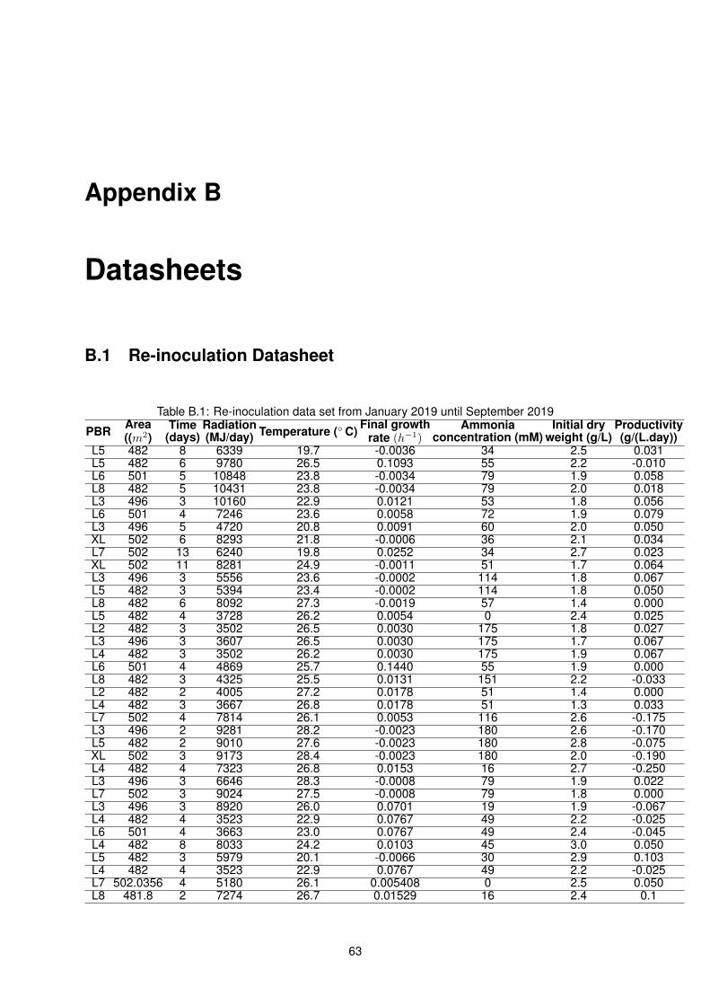
Appendix B
Datasheets
B.1 Re-inoculation Datasheet
Table B.1: Re-inoculation data set from January 2019 until September 2019
PBR Area((m2)
Time(days)
Radiation(MJ/day) Temperature (◦ C) Final growth
rate (h−1)Ammonia
concentration (mM)Initial dry
weight (g/L)Productivity(g/(L.day))
L5 482 8 6339 19.7 -0.0036 34 2.5 0.031L5 482 6 9780 26.5 0.1093 55 2.2 -0.010L6 501 5 10848 23.8 -0.0034 79 1.9 0.058L8 482 5 10431 23.8 -0.0034 79 2.0 0.018L3 496 3 10160 22.9 0.0121 53 1.8 0.056L6 501 4 7246 23.6 0.0058 72 1.9 0.079L3 496 5 4720 20.8 0.0091 60 2.0 0.050XL 502 6 8293 21.8 -0.0006 36 2.1 0.034L7 502 13 6240 19.8 0.0252 34 2.7 0.023XL 502 11 8281 24.9 -0.0011 51 1.7 0.064L3 496 3 5556 23.6 -0.0002 114 1.8 0.067L5 482 3 5394 23.4 -0.0002 114 1.8 0.050L8 482 6 8092 27.3 -0.0019 57 1.4 0.000L5 482 4 3728 26.2 0.0054 0 2.4 0.025L2 482 3 3502 26.5 0.0030 175 1.8 0.027L3 496 3 3607 26.5 0.0030 175 1.7 0.067L4 482 3 3502 26.2 0.0030 175 1.9 0.067L6 501 4 4869 25.7 0.1440 55 1.9 0.000L8 482 3 4325 25.5 0.0131 151 2.2 -0.033L2 482 2 4005 27.2 0.0178 51 1.4 0.000L4 482 3 3667 26.8 0.0178 51 1.3 0.033L7 502 4 7814 26.1 0.0053 116 2.6 -0.175L3 496 2 9281 28.2 -0.0023 180 2.6 -0.170L5 482 2 9010 27.6 -0.0023 180 2.8 -0.075XL 502 3 9173 28.4 -0.0023 180 2.0 -0.190L4 482 4 7323 26.8 0.0153 16 2.7 -0.250L3 496 3 6646 28.3 -0.0008 79 1.9 0.022L7 502 3 9024 27.5 -0.0008 79 1.8 0.000L3 496 3 8920 26.0 0.0701 19 1.9 -0.067L4 482 4 3523 22.9 0.0767 49 2.2 -0.025L6 501 4 3663 23.0 0.0767 49 2.4 -0.045L4 482 8 8033 24.2 0.0103 45 3.0 0.050L5 482 3 5979 20.1 -0.0066 30 2.9 0.103L4 482 4 3523 22.9 0.0767 49 2.2 -0.025L7 502.0356 4 5180 26.1 0.005408 0 2.5 0.050L8 481.8 2 7274 26.7 0.01529 16 2.4 0.1
63

B.2 Inoculation Datasheet
Table B.2: Inoculation data set from January 2018 until September 2019.
PBR Area((m2)
Time(days)
Radiation(MJ/day) Temperature (◦ C) Final growth
rate (h−1)Ammonia
concentration (mM)Initial dry
weight (g/L)Productivity(g/(L.day))
L3 496 6 49756 21.7 -0.0006 36 1.3 0.017L4 482 13 77848 19.4 0.0252 34 2.2 -0.004L6 501 8 66833 23.9 0.0103 45 1.7 0.073L7 502 11 92153 24.4 -0.0011 51 1.1 0.041L8 482 7 58364 22.4 0.0313 24 1.7 0.090XL 502 14 103177 20.8 -0.0036 NA 1.4 0.038XL 502 7 60816 22.4 0.0313 24 1.6 0.078L8 482 5 52083 26.9 0.0077 50 1.6 0.080XL 502 5 54271 28.7 0.0077 50 1.5 0.093L2 482 4 27869 23.9 0.0058 72 1.8 0.025L5 482 3 14701 20.7 0.0091 NA 1.7 0.048L5 482 14 98391 20.8 0.0020 26 2.0 0.038L3 496 14 101343 20.8 0.0020 26 1.8 0.040L8 482 5 21392 23.3 0.0254 32 1.2 0.033L6 501 6 50495 27.5 -0.0019 57 1.3 0.075L4 482 6 48553 27.1 -0.0019 57 1.3 0.083L2 482 3 14226 23.5 0.0045 117 1.0 0.067L3 496 3 14652 25.7 0.0045 117 1.0 0.050L5 482 3 14226 25.5 0.0045 117 0.8 0.050L7 502 3 14823 25.3 0.0045 117 1.1 0.117L6 501 3 17893 26.4 -0.0008 111 0.6 0.053L8 482 3 22957 26.2 -0.0008 111 0.9 0.042XL 502 5 28389 25.5 0.0131 151 0.9 0.040L3 496 6 29143 27.3 0.0178 51 1.4 -0.083L2 482 5 46888 27.6 0.0513 12 0.9 0.253L6 501 5 41263 26.3 0.0053 116 1.7 0.002L5 482 3 26760 27.7 -0.0008 79 1.5 0.117XL 502 4 33471 27.1 -0.0025 27 1.2 -0.025L2 482 4 32496 26.4 -0.0025 27 1.4 -0.050L4 482 4 32400 27.1 0.0071 49 1.2 0.000L6 501 4 33696 26.6 0.0071 49 1.4 -0.063L7 502 6 30117 22.8 0.0179 16 1.8 -0.017L8 482 6 28903 23.2 0.0179 16 2.0 -0.117L5 482 6 24485 23.2 0.0767 49 1.9 0.002L5 482 14 2643 16.7 0.0177 43 2.2 -0.005L8 482 8 2662 14.0 0.0308 172 1.1 0.005L7 502 22 2560 14.5 0.0535 95 1.7 -0.034L5 482 6 3045 14.7 -0.0078 157 2.0 -0.038L2 482 5 3894 12.0 0.0177 138 1.3 -0.040L3 496 5 4011 12.5 0.0177 138 1.3 -0.020L4 482 6 4982 20.2 -0.0016 69 0.6 0.021L3 496 6 5131 20.4 -0.0016 69 0.5 0.003L5 482 6 4982 20.4 -0.0016 69 0.7 0.016L7 502 6 5191 19.6 -0.0016 69 0.6 0.028L2 482 8 8984 25.5 0.0070 37 1.4 0.039L8 482 6 8734 25.3 0.0070 37 1.2 0.059L5 482 3 5708 25.0 -0.0110 29 1.4 0.000XL 502 3 5948 25.4 -0.0110 29 1.2 0.000L6 501 6 7682 23.5 0.0040 34 2.2 -0.033XL 502 9 6860 25.9 -0.0032 26 1.5 0.056L8 482 6 6748 26.0 -0.0032 26 1.8 0.092L4 482 8 8670 27.9 -0.0941 28 1.4 -0.034L2 482 8 8670 26.0 -0.0941 28 1.4 -0.025L5 482 6 6644 23.3 0.0069 53 2.0 0.042
64

B.3 Code for cross-validation
Figure B.1: Code of the hold out validation method for the two inoculation systems.
65

B.4 Results from MLR model
Figure B.2: Generalized least squares results for re-inoculation systems.
Figure B.3: Ordinary least squares results for inoculation systems.
66